A new computerized x-ray densitometricsystem for tree-ring analysis

Item Type text; Thesis-Reproduction (electronic)

Authors McCord, V. Alexander S.

Publisher The University of Arizona.

Rights Copyright © is held by the author. Digital access to this materialis made possible by the University Libraries, University of Arizona.Further transmission, reproduction or presentation (such aspublic display or performance) of protected items is prohibitedexcept with permission of the author.

Download date 06/06/2018 18:32:46

Link to Item http://hdl.handle.net/10150/557992

A NEW COMPUTERIZED X-RAY DENSITOMETRIC SYSTEMFOR TREE-RING ANALYSIS

byVIRGIL ALEXANDER STUART MCCORD

A Thesis Submitted to the Faculty of theDEPARTMENT OF GEOSCIENCES

In Partial Fulfillment of the Requirements For the Degree ofMASTER OF SCIENCE

In the Graduate CollegeTHE UNIVERSITY OF ARIZONA

1 9 8 4

STATEMENT BY AUTHOR

This thesis has been submitted in partial fulfillment of requirements for an advanced degree at the University of Arizona and is deposited in the University Library to be made available to borrowers under rules of the Library.

Brief quotations from this thesis are allowable without special permission, provided that accurate acknowledgment of source is made. Requests for permission for extended quotation from or reproduction of this manuscript in whole or in part may be granted by the head of the major department or the Dean of the Graduate College when in his judgment the proposed use of the material is in the interests of scholarship. In all other instances, however, permission must be obtained from the author.

SIGNED ill. T~>.

APPROVAL BY THESIS DIRECTOR This thesis has been approved on the date shown below:

i/, ^ /l̂<— / 3-̂ y/V. C. LAMARCHE, JR.

Professor of DendrochronologyDate

ACKNOWLEDGMENTS

This thesis would not have been possible without the help and support of many friends and colleagues. Financial support and facilities were provided by the Laboratory of Tree-Ring Research, University of Arizona. I especially thank Valmore C. LaMarche, Jr., my major advisor, for continuing advice and direction throughout the project. He and my committee members Marvin A. Stokes and Austin Long, and graduate student Susanmarie Clark critically read all or parts of the manuscript, and provided helpful comments and suggestions. Martin R. Rose carefully proofread the final copy. William J. Robinson helped with computerization problems and with the design and acquisition of equipment. David C. Steinke provided valuable help in the design and construction of electronic equipment. Michael S. McCarthy and Paige W. Bausman assisted with some of the computer programming. Thomas P. Harlan helped to produce the photographic illustrations. I am especially indebted to Susanmarie Clark for her untiring help on the drafting and preparation of nearly all of the illustrations. I thank Trevor Bird, Edward R. Cook, Harold C. Fritts, Richard L. Holmes, and Malcolm K. Cleaveland for valuable discussions and suggestions. I thank all those who helped me; any errors that remain, however, are my own.

iii

TABLE OF CONTENTS

LIST OF ILLUSTRATIONS........................... ....A B S T R A C T ..................................... viii

1. INTRODUCTION .................................... 12. SAMPLE COLLECTION AND PREPARATION ............... 8

Field c o l l e c t i o n ........................ 8Preparation of Cores for Radiography . . . . 113. RADIOGRAPHY OF C O R E S ..........................28

General Methods in U s e ....................28Static Method ........................... 28Scanning Method ........................ 32Comparison of Scanning and Static Methods . 32

Scanning Method .............................. 33E q u i p m e n t .............................33Uniformity of X-ray Dosage ............... 36

Film and Exposure..........................39F i l m ...................................39Exposure Criteria ........................ 40

Exposure Procedure .................. . . . 464. OPTICAL DENSITOMETRY ........................... 47

Optical Microdensitometer .................. 47Recording System ........................... 52Signal Amplification ........................ 54External Drive System and Computer Interface . 56Computer Software ........................... 60Current System Limitations .................. 61

Scan Length and Film Positioning . . . . 61Non-rotatable Seconday Apertures . . . . 63Densitometer Resolution .................. 67

Other Possible Approaches .................. 71Single-beam Densitometer ............... 71Video Image Analyzer....................72

Page

iv

V

TABLE OF CONTENTS— Continued

5. DATA MANIPULATION AND CALIBRATION.................. 74Program CALIBRATE . 75

Cellulose Acetate Calibration Standard . . 75Curve-fitting with Interactive Graphics . 77

Identification of Ring Boundaries ............ 80Search for Latewood Maximum Densities—Program GETMAX ........................ 80

Editing with Interactive Graphics—Program BOUNDARY CHECK ............... 86

Scan Merging and Data Transformation—Program MATCH . 89Other Programs— GETMIN, BC-MIN, AVDEN . . 94

6. SUMMARY AND DISCUSSION...............................97Sample Collection and Preparation . . . . . 97Radiography.....................................98Optical Densitometry ........................ 100

Sample Rate................................ 101Limited Length of Scan T a b l e .............. 102Densitometer Resolution . . . . . . . 103

Data Manipulation and Calibration ............ 105Calibration ............ . . . . . . 105Data Manipulation.......................... 107Computer Limitations ..................... 108

APPENDIX A: CIRCUIT DIAGRAMS .................. 114APPENDIX B: SOFTWARE ........................... 118LIST OF REFERENCES................................ 147

Page

LIST OF ILLUSTRATIONS

1.1 Block diagram of X-ray densitometryfacility ................................. 5

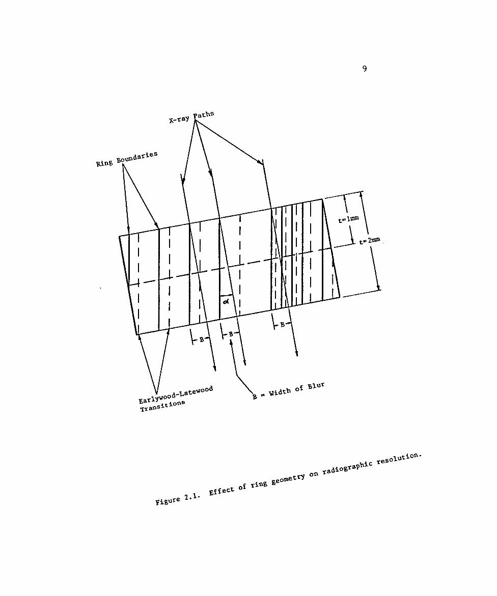
2.1 Effect of ring geometry on radiographicresolution ................................. 9

2.2 Core mounting techniquefor X-ray densitometry ..................... 15

2.3 Photomicrograph of coremachined by double-bladed s a w ............... 18

2.4 Tangential view of machinedand polished c o r e ........................... 19

2.5 Plot generated by Apple computer comparingminimum earlywood densities ofsanded and unsanded specimen ............... 21

2.6 Partial removal of sanding dustby sonication in ac e t o n e ..................... 23

2.7 Results of acetone extractionof resinous material ..................... 27

3.1 Geometric relationshipof X-ray source to target..................... 29

3.2 Static and scanning radiographic techniques . 303.3 X-ray scanning apparatus ..................... 343.4 Core specimen on carriage

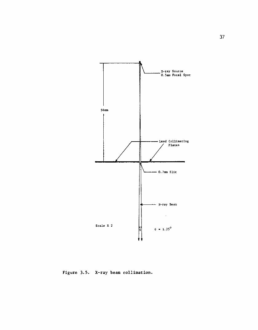
ready for radiography........................ 353.5 X-ray beam collimation........................ 373.6 Calculated X-ray absorption curves . . . . 423.7 Densitometer scan of radiograph

of cellulose acetate step-wedge ............ 45

Figure Page

vi

vii

LIST OF ILLUSTRATIONS— Continued4.1 Joyce-Loebl Mk III CS

optical microdensitometer . . . 484.2 Optical densitometry

measuring and recording system 494.3 Schematic diagram, single-beam and double-

optical densitometer principles . .•beam

514.4 Amplified and unamplified

densitometer output signals 554.5 Densitometer table drive system,

showing lead-screw mechanism and optical shaft encoder . 58

4.6 Chart recording showing computer file identification marks ............... 62

4.7 Theoretical resolution of 0.04mm X 0 scanning "box" ...............

.4mm65

4.8 Relationship of scanning "box" to slanted ring boundary 66

4.9 Radiograph of poorly aligned narrow rings 684.10 Radiograph of slightly damaged rings 705.1 Calibration step wedge data:

graphic fit of horizontal lines . 795.2 Portion of dated and annotated strip chart recording . . . . 825.3 Chart recording showing "buffer zone

used by peak detection programn

845.4 Portions of chart recordings showing differing

density characteristics of two trees 855.5 Screen display of two successive

BOUNDARY CHECK plots . . . . 875.6 BOUNDARY CHECK editing process 90

ABSTRACT

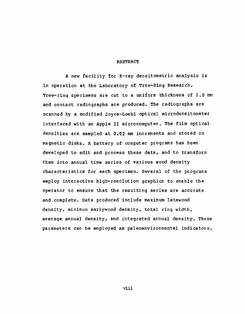
A new facility for X-ray densitometric analysis is in operation at the Laboratory of Tree-Ring Research. Tree-ring specimens are cut to a uniform thickness of 1.0 mm and contact radiographs are produced. The radiographs are scanned by a modified Joyce-Loebl optical microdensitometer interfaced with an Apple II microcomputer. The film optical densities are sampled at 0.02 mm increments and stored on magnetic disks. A battery of computer programs has been developed to edit and process these data, and to transform them into annual time series of various wood density characteristics for each specimen. Several of the programs employ interactive high-resolution graphics to enable the operator to ensure that the resulting series are accurate and complete. Data produced include maximum latewood density, minimum earlywood density, total ring width, average annual density, and integrated annual density. These parameters can be employed as paleoenvironmental indicators.

viii

CHAPTER 1

INTRODUCTION

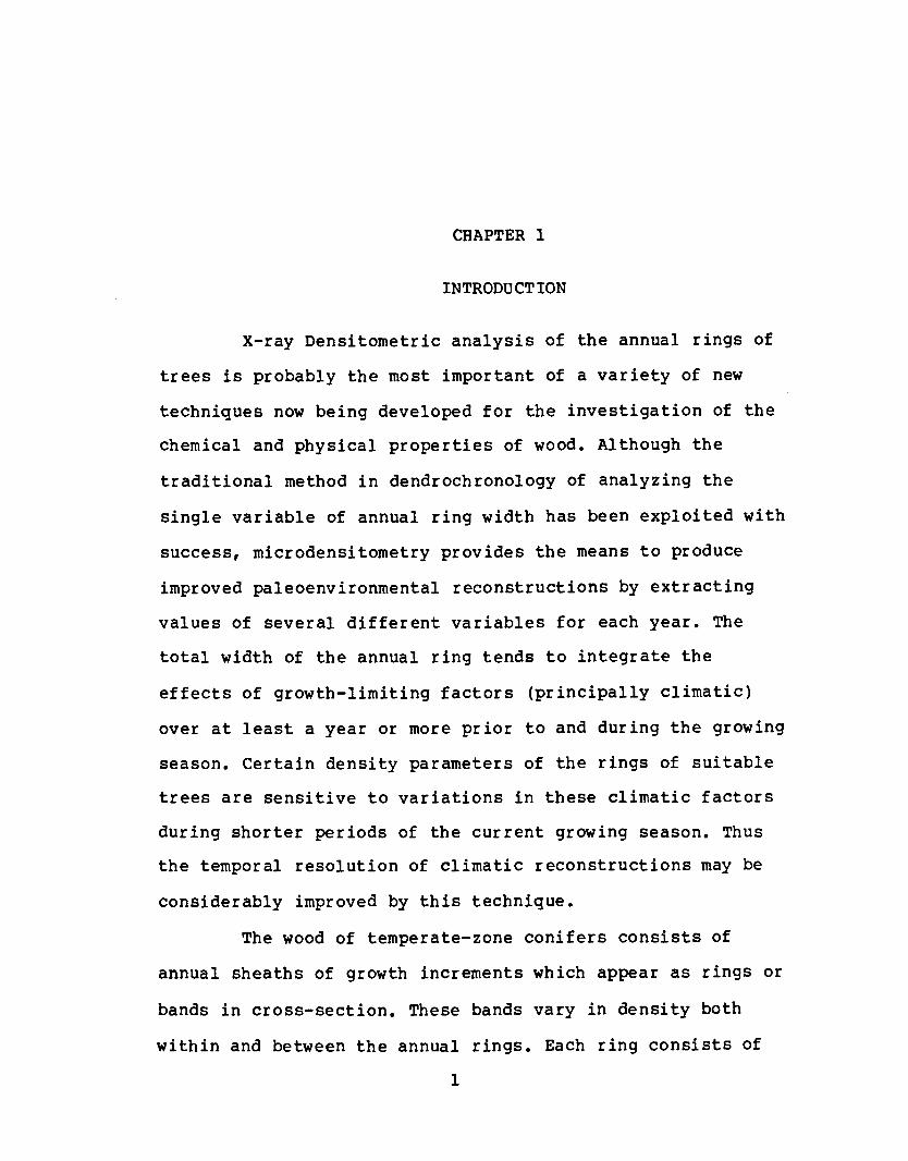
X-ray Densitometric analysis of the annual rings of trees is probably the most important of a variety of new techniques now being developed for the investigation of the chemical and physical properties of wood. Although the traditional method in dendrochronology of analyzing the single variable of annual ring width has been exploited with success, microdensitometry provides the means to produce improved paleoenvironmental reconstructions by extracting values of several different variables for each year. The total width of the annual ring tends to integrate the effects of growth-limiting factors (principally climatic) over at least a year or more prior to and during the growing season. Certain density parameters of the rings of suitable trees are sensitive to variations in these climatic factors during shorter periods of the current growing season. Thus the temporal resolution of climatic reconstructions may be considerably improved by this technique.

The wood of temperate-zone conifers consists of annual sheaths of growth increments which appear as rings or bands in cross-section. These bands vary in density both within and between the annual rings. Each ring consists of

1

2an inner low-density portion called earlywood, composed mainly of large-diameter thin-walled cells, and an outer higher-density portion called latewood, composed of small diameter thicker-walled cells. Differences in cell-wall diameter and cell-wall thickness are closely reflected in the density profile of the annual ring. Since cell wall diameter and cell wall thickness are partly controlled by external environmental conditions, analysis of annual sequences of wood density variations can be used for the reconstruction of these environmental variables (Conkey, 1982). For example, in certain conifer stands the maximum latewood density of the annual ring is strongly related to late summer temperature (Parker, 1976, Schweingruber et al, 1978) .

X-ray densitometry provides an efficient and accurate method of measuring and recording these intra-annual and interannual wood density variations (Polge, 1966). The technique is based on the relationship of wood density to the absorption of X-radiation. A thin wood specimen of uniform thickness (usually from 1 mm to 6 mm) is placed on a sheet of film and exposed to a uniform dosage of low-energy ("soft") X-radiation in most applications. The degree of X-ray absorption is proportional to the density of the wood, producing an X-ray negative in which the optical density of the radiographic image is inversely proportional

3

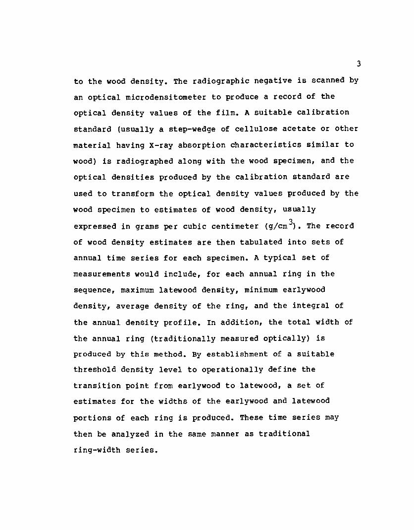
to the wood density. The radiographic negative is scanned by an optical micr©densitometer to produce a record of the optical density values of the film. A suitable calibration standard (usually a step-wedge of cellulose acetate or other material having X-ray absorption characteristics similar to wood) is radiographed along with the wood specimen, and the optical densities produced by the calibration standard are used to transform the optical density values produced by the wood specimen to estimates of wood density, usually expressed in grams per cubic centimeter (g/cm ). The record of wood density estimates are then tabulated into sets of annual time series for each specimen. A typical set of measurements would include, for each annual ring in the sequence, maximum latewood density, minimum earlywood density, average density of the ring, and the integral of the annual density profile. In addition, the total width of the annual ring (traditionally measured optically) is produced by this method. By establishment of a suitable threshold density level to operationally define the transition point from earlywood to latewood, a set of estimates for the widths of the earlywood and latewood portions of each ring is produced. These time series may then be analyzed in the same manner as traditional ring-width series.

X-radiography and X-ray densitometry was first applied to wood quality studies in Switzerland (Lenz, 1957) and France (Polge, 1965, 1966), and later at other forest-products laboratories in Canada, Australia, and the United States (eg Parker and Henoch, 1971? Lenz, Schar, and Schweingruber, 1976? Rudman, 1968, 1969? Echols, 1970, 1972, 1973). The technique has been subsequently applied to dendrochronological problems, including the reconstruction of environmental histories (Parker and Henoch, 1972? Cleaveland, 1975,1983? Schweingruber et al, 1978? Conkey 1979, 1982), cross-dating of width-complacent series (Jones and Parker, 1970? Clague, Jozsa, and Parker, 1982), and to the recognition of short-term meteorological events within the growing season, reflected as density anomalies within the annual ring (Schweingruber, 1979).

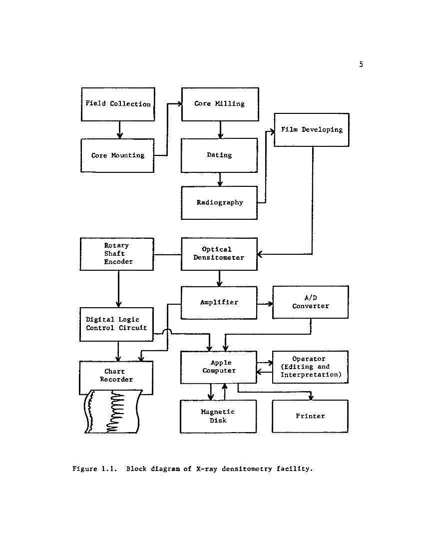
A facility for X-ray densitometric analysis of dendrochronological material has recently become fully operational at the University of Arizona Laboratory of Tree-Ring Research (Figure 1.1). Its principal purpose is to evaluate the potential scope of the use of X-ray densitometry in paleoclimatic studies, particularly of environmentally stressed sites. Extracting densitometric information is a complex procedure and requires careful consideration of each step in the process. Both theoretical and technical problems place limitations on the

4

5

ChartRecorder

Encoder

RotaryShaft

Operator (Editing and Interpretation)

Field Collection

Core Mounting

Printer

Converter

AppleComputer

Film Developing

Digital Logic Control Circuit

DensitometerOptical

Amplifier

MagneticDisk

Radiography

Core Milling

Dating

Figure 1.1. Block diagram of X-ray densitometry facility.

interpretation and application of densitometric data to environmental reconstruction.

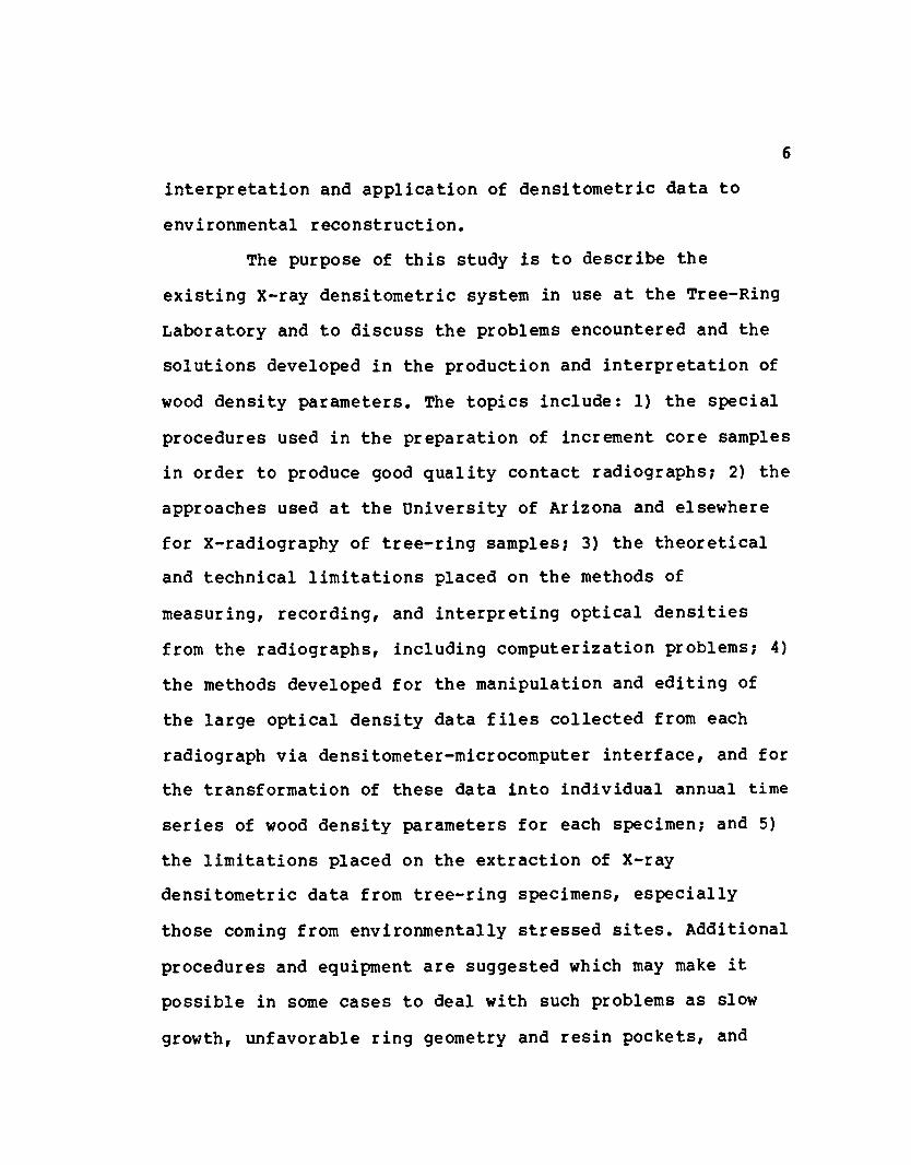
The purpose of this study is to describe the existing X-ray densitometric system in use at the Tree-Ring Laboratory and to discuss the problems encountered and the solutions developed in the production and interpretation of wood density parameters. The topics include: 1) the special procedures used in the preparation of increment core samples in order to produce good quality contact radiographs; 2) the approaches used at the University of Arizona and elsewhere for X-radiography of tree-ring samples? 3) the theoretical and technical limitations placed on the methods of measuring, recording, and interpreting optical densities from the radiographs, including computerization problems; 4) the methods developed for the manipulation and editing of the large optical density data files collected from each radiograph via densitometer-microcomputer interface, and for the transformation of these data into individual annual time series of wood density parameters for each specimen? and 5) the limitations placed on the extraction of X-ray densitometric data from tree-ring specimens, especially those coming from environmentally stressed sites. Additional procedures and equipment are suggested which may make it possible in some cases to deal with such problems as slow growth, unfavorable ring geometry and resin pockets, and

6

7with microcomputer limitations, including memory size, program complexity and flexibility, and limitations involved in the use of high-resolution graphics.

CHAPTER 2

SAMPLE COLLECTION AND PREPARATION

Field CollectionField collection, storage, and transport of cores is

done in essentially the same manner as collection for ring-width studies. Particular attention is given to ensuring that the cores are taken as nearly as possible at right angles to both the tangential and longitudinal dimensions of the tree, so that when the core is prepared for radiography the wood fibers (tracheid cells) will be oriented perpendicularly to the long axis of the core, and the x-rays will subsequently pass through the specimen parallel to the fibers. Otherwise, the portion of the beam at any one point on the core may pass through two or more adjacent fibers (of different density) and its absorption will be due to some combination of densities of the various fibers, rather than the true density of the wood at that point. As can be seen in Figure 2.1, this leads to a "blur", or zone of poor definition. Many trees growing on dendrochronologically sensitive sites exhibit only moderate to poor parallelism of fibers and therefore no matter what angle of entry is selected for the borer, some of the fibers are almost invariably oriented at other than right angles to

8

9

of

10

the axis of the core, often varying from ten to twenty degrees and sometimes up to thirty degrees or even more along a single radius. For this reason the use of special equipment for clamping the borer at a precise right angle to the bark of the tree is not felt to be worth the extra expense, time, and inconvenience involved. All one can really do is to make a decision as to what coring angle is likely to cross the largest number of ring boundaries at an angle reasonably close to ninety degrees. Multiple cores may be required on some radii.

The problem of fiber orientation is more critical with narrow rings, where there is the danger that the x-ray path through the core must pass through two or more annual rings (Figure 2.1). Since the rings near the outer part of a tree are usually narrower than the rings in the center, it is wise to hold the borer perpendicular to the bark of the tree. This angle can be approximated by having an assistant hold the handle of one borer flush against the tree with the bit pointed away from the tree, and using this as a visual guide for starting a second borer to extract the core. If field examination of the core shows a large number of rings oriented at other than right angles to the axis of the core, then the angle may be adjusted by eye with reference to the guide borer, and a second core taken. It is generally good practice to take two or more cores from each radius at

11slightly different angles, especially if there is very much variation in fiber orientation along the radius. More flexibility then exists when selecting cores to be prepared for radiography.

A detailed analysis of site selection for X-ray densitometry involves consideration of complex and interrelated environmental and biological variables, and is outside the scope of this paper. Some general guidelines can be suggested, however. Trees selected should exhibit an observable degree of year-to-year variation in density of the latewood band, as determined by macroscopic field examination. Degree of coloration and relative width of the latewood band are the most useful field criteria. Further, the annual rings should be wide enough so that adequate radiographic resolution can be achieved in the laboratory.

Preparation of Cores for RadiographyCores are mounted and machined to a uniform

thickness, usually between one and two millimeters, depending on the width of the rings and the degree of radiographic resolution required. Machining to a constant thickness is essential since the absorption of X-radiation is related not only to the density and chemical composition of the material through which it passes, but also to its thickness. The chemical composition of the wood, insofar as it affects the absorption of X-rays, is assumed to vary only

12

insignificantly throughout the radius of a tree. Then if the thickness of a specimen is made constant, any variation in x-ray absorption may be attributed solely to variation in density along the core.

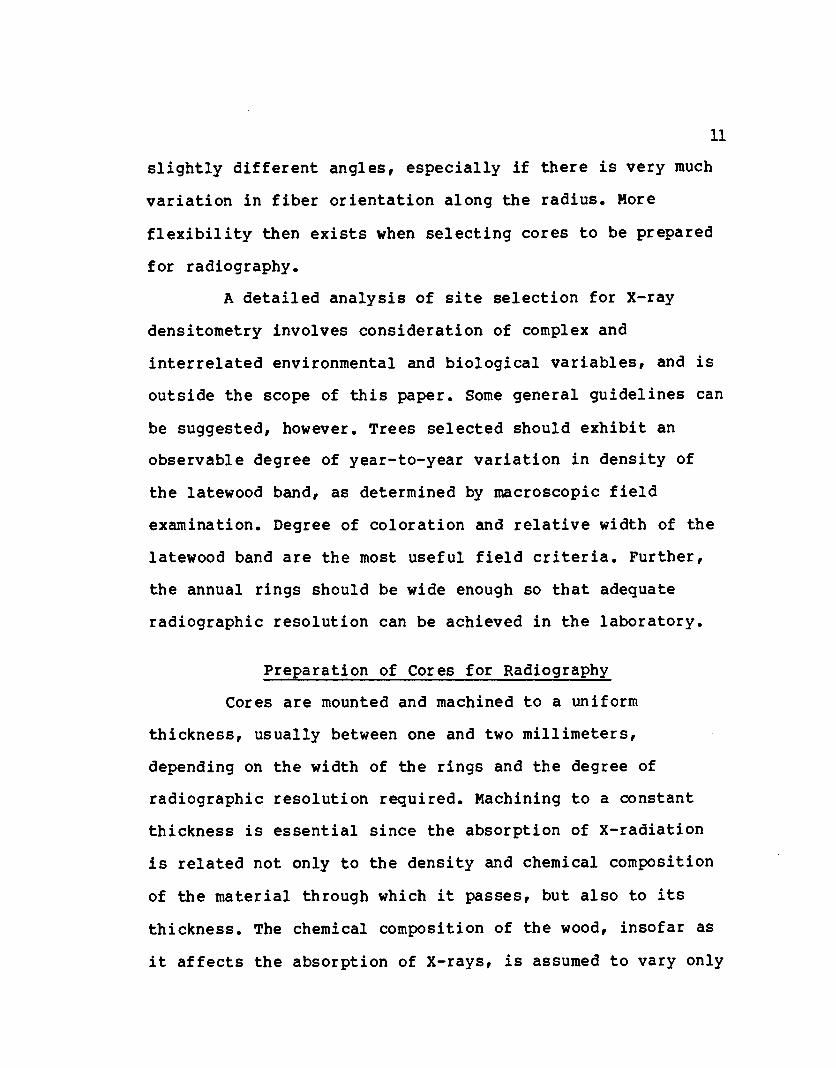
The parallax problem arising from non-parallel wood fiber orientation tends to produce a shadowing effect in the radiograph, resulting in poor radiographic resolution. The radiographs have "fuzzy" ring boundaries, and apparent densities of latewood maxima are less than their true densities. The narrower the rings are, the more serious this effect becomes. In extreme cases, the individual ring boundaries cannot be identified from the radiograph. Radiographic resolution is inversely related to sample thickness, and therefore it is desirable that the cores be machined as thinly as practically possible in order to maximize resolution (Figure 2.1). Since many dendrochronologically sensitive trees have at least some rings which are less than one millimeter or even less than one-half millimeter in width, it would be desirable to prepare cores for radiography having a uniform thickness of considerably less than one millimeter.

There are, however, certain factors which place limitations on how thin the specimen may be cut. In order to maintain a constant thickness, the specimen thickness must be large in comparison to any roughness of the surface.

13

If the surfacing technique employed produces a roughness on the order of 0.1 mm, then the specimen must be about 2 mm thick in order to maintain the desired thickness within 5%. Obviously, it is advantageous to produce as smooth a surface as possible. Another limitation to the thickness of the specimen is the very low mechanical strength of wood when cut across the grain. Cores cut to the order of one or two millimeters have practically no mechanical strength and are likely to be destroyed by any ordinary machining technique.

Two basic methods of machining cores have been used at this laboratory: the double-bladed saw method based on the design of Kusec (1972), and the router-planer method based on the design of Olsen, Arganbright, and Rygiewicz (1978). The router-planer method is now routinely used. Problems with feeding the specimen into the double-bladed saw, maintenance of blade alignment, resin buildup on the blades, and microscopic dulling of the teeth after a few cuts contributed to excessive vibration and heat buildup, which resulted in "chattermarks" and rough surfaces and occasional charring or shattering of the specimen. These problems were never fully overcome.

The router-planer method of machining cores has proven to be much more satisfactory. The machine consists of a standard workshop router fitted with a spiral 2-fluted cutter and mounted above an adjustable-height bed.

14

The mounted specimen is passed between the bed and cutter by a pair of variable-speed motor-driven infeed and outfeed rollers. A small thickness of the core and mount is thus planed off by the router bit along the length of its flutes, producing a very flat surface. Top and bottom of the mounted cores are alternately planed until the desired thickness is reached.

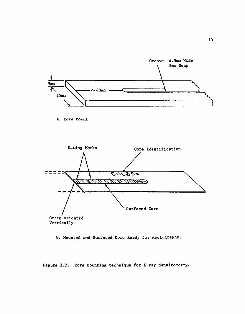
The core mount is made of a strip of basswood or poplar, 25 mm wide by about 5 mm thick (Figure 2.2) . A deep groove is routed throughout most of the length of this strip, using a standard 3/16 inch router bit and a special jig constructed for the purpose. The core is then pressed and glued into the groove with ordinary white glue (PVA - polyvinyl acetate, such as Elmer's), taking care to ensure that the tracheids are oriented vertically. The cores and mounts are then placed on a flat surface, covered with wax paper, weighted with a heavy aluminum plate, and allowed to dry overnight. In some cases the cores may become twisted during extraction from the tree, and it is not possible to orient all the fibers vertically. This condition can usually be corrected by carefully steaming the core over a low-pressure steam jet until the fibers have been softened enough to gently untwist the core before pressing and glueing it into the mount.

15

Groove 4.5mm Wide3mm Deep

a. Core Mount

Dating Marks Core Identification

<5>W^<E.'BVk\\ \\\ \vV

Surfaced Core

Grain OrientedVertically

b. Mounted and Surfaced Core Ready for Radiography.

Figure 2.2. Core mounting technique for X-ray densitometry.

Basswood was selected for core mount material for several reasons. It has straight grain and resists warping when cut into thin strips, and is relatively soft and easily worked. Its low resin content reduces resin buildup and fouling of the router bit, and it is reasonably low in cost. Poplar also gives good results and appears to have similar machining properties. Either poplar or basswood is used, depending on current local availability and price.

White glue does an acceptable job of holding the core in the mount during the machining process and subsequent handling, and it is low in cost and readily available. Occasionally it is desirable to remove one side of the mount after machining in order to inspect the core from the side and ascertain the degree of verticality of the fibers. The fact that white glue may be softened by soaking in water facilitates this process.

Cores machined by the router-planer are consistently cut to a uniform thickness, and can usually be cut to a thickness of two millimeters or even less without damage to the core. Some damage is occasionally done to parts of the core if it is cut too thin, and the process is rather slow, but the quality of the surface is decidedly better than that obtainable with the twin-bladed saw, feeding problems are considerably reduced, and there is much less danger of shattering, gouging, or charring the specimen.

16

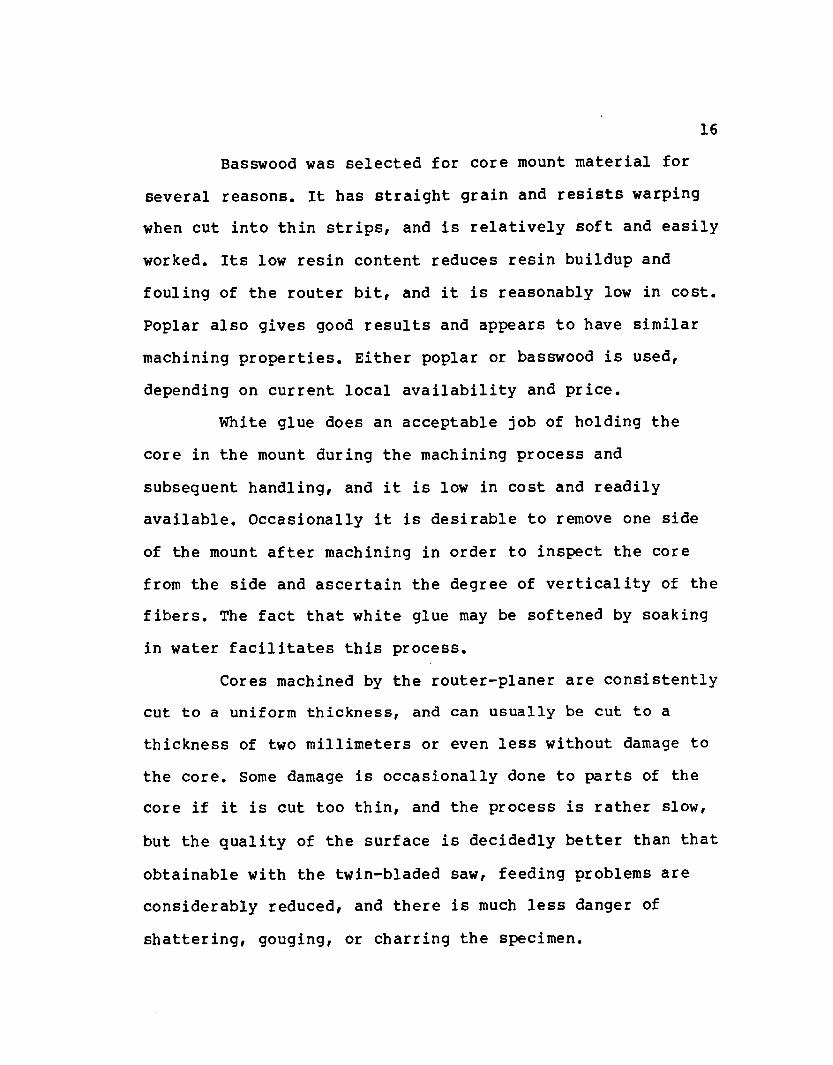
The machined surface is not perfect, however, and further treatment is usually necessary. When viewed under the microscope, it can be seen that the individual cells and the ring bounaries are not discernable, due to the roughness of the surface. This surface is not suitable for optical cross-dating of the specimen. A polished surface is essential to reveal all of the ring boundaries when examined with a microscope. As can be seen in Figure 2.3, many of the planed specimens would be impossible to date on an unpolished surface.

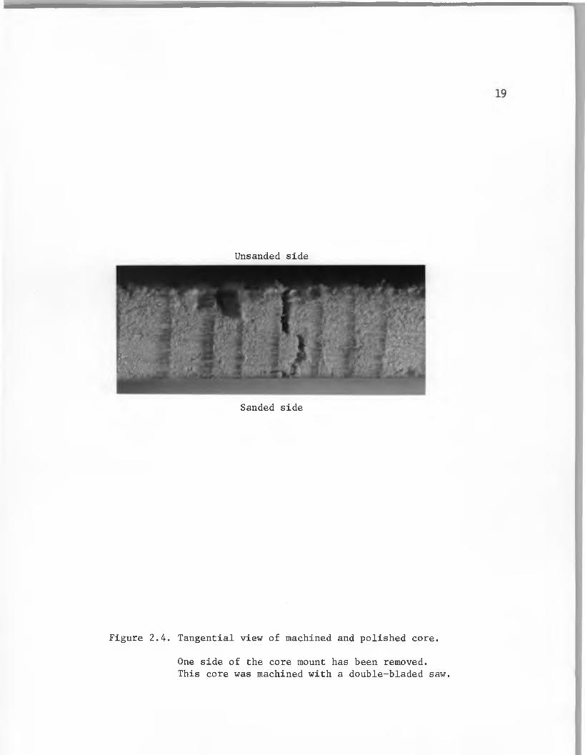
The standard practice in dendrochronology is to produce a polished surface by sanding the specimen (Stokes and Smiley 1968, p. 46). When cores are sanded, the earlywood cells tend to become clogged with sanding dust. This condition theoretically has the effect of causing the measured minimum earlywood density to be falsely high (Olson, Arganbright, and Rygiewicz, 1978, p. 34). However, it is apparent from Figure 2.4 that in many cases the earlywood fibers of machined cores are not cleanly cut by the saw or router, but are merely pushed aside and torn.This condition has the same effect on measured earlywood density as sanding dust clogging the pores: in either case more material is present than would be accounted for by the nominal thickness. Note also that the sanded side of the core shown in Figure 2.4 is much smoother and flatter than

17

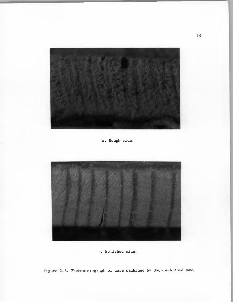
a. Rough side.

b. Polished side.

Photomicrograph of core machined by double-bladed

Unsanded side

mWi-

#Sanded side

Figure 2.4. Tangential view of machined and polished core.

One side of the core mount has been removed.This core was machined with a double-bladed saw.

20

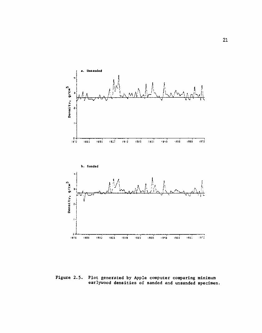
the machined side, producing a more uniform thickness.Sanded cores sliced at a shallow angle with a razor blade show that the impregnation of sanding dust is confined to a very thin zone near the surface of the core. This zone is quite thin compared with the thickness of most of our samples (1 mm). Figure 2.5 shows comparative plots of minimum earlywood densities from radiographs taken before and after sanding the surface of a specimen. Some variation is observed, but this is felt to be within the range of variation expected to be encountered from one file of cells to the next.

In order to produce a suitable surface the machined core is sanded on both sides using 100 grit garnet sandpaper and a small hand-held Porter-Cable "Speedblock" orbital sander until the final thickness is obtained. When the earlywood cell walls become visible with a hand lens, finer grades of sandpaper are used until the desired polish is attained. It is important to use the 100 grit paper until the earlywood cells are visible, because if the switch to finer grades is made too soon, one is merely polishing the bent-over fibers of the rough surface. Then the individual cells and the ring boundaries will still not be visible, and the entire sanding process must be repeated. Usually 500 grit carborundum sandpaper is the finest grade used. This process produces an excellent surface for dating

21

a. Unsanded

! •-I

I -

H---------,- - - - - - - 1- - - - - - - >------- r;E:: ;BS: i b s c is:: isi: !923 f SHD i 55D i si:

b. Sanded

iM.A/; r izv\

„ n,■ ■̂ yy/y \ y ̂Wi A

S . Ji

yAnr-^7lH

I -

5J------------ ,------------;------------,------------rIBID IBSB IBS: (SCO 1210 !S22 ',5 30 I SH D iss: i s e :

Figure 2.5. Plot generated by Apple computer comparing minimum earlywood densities of sanded and unsanded specimen.

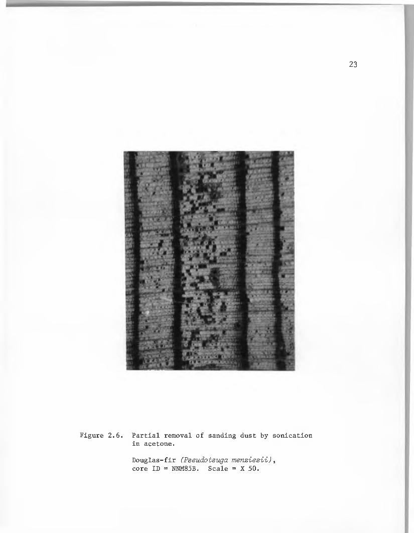
22and a very uniform specimen thickness. Placing the specimen in an ultrasonic bath of acetone for about ten minutes will remove the sanding dust from some of the earlywood cells, but the process is incomplete and not very uniform (Figure 2.6). Longer and more vigorous sonication on thinner cores might produce more satisfactory results.

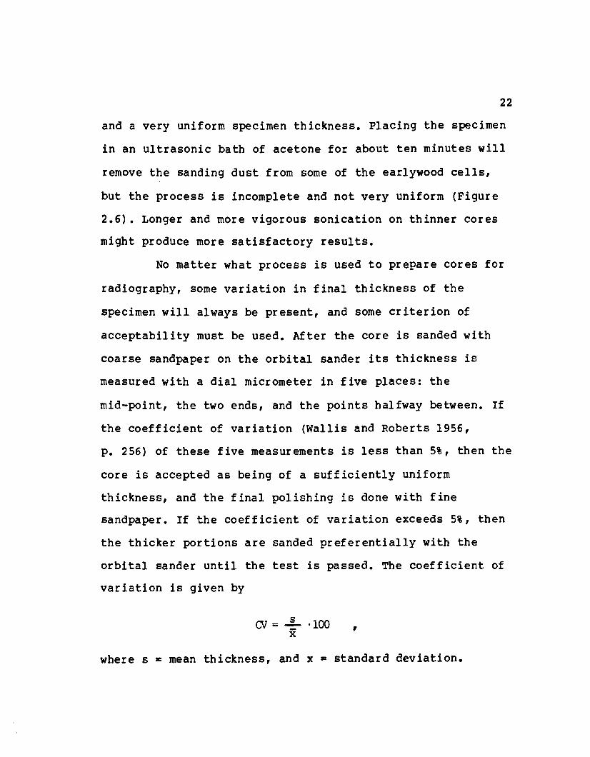
No matter what process is used to prepare cores for radiography, some variation in final thickness of the specimen will always be present, and some criterion of acceptability must be used. After the core is sanded with coarse sandpaper on the orbital sander its thickness is measured with a dial micrometer in five places: the mid-point, the two ends, and the points halfway between. If the coefficient of variation (Wallis and Roberts 1956, p. 256) of these five measurements is less than 5%, then the core is accepted as being of a sufficiently uniform thickness, and the final polishing is done with fine sandpaper. If the coefficient of variation exceeds 5%, then the thicker portions are sanded preferentially with the orbital sander until the test is passed. The coefficient of variation is given by

CV = _s_x •100 r

where s = mean thickness, and x = standard deviation

23

Figure 2.6. Partial removal of sanding dust by sonication in acetone.

Douglas-fir (Pseudotsuga menziesii), core ID = NNM85B. Scale = X 50.

24

The coefficient of variation is a measure of relative variation, which in this case expresses the standard deviation of the core thickness as a percentage of the mean, and is therefore independent of the actual specimen thickness. Therefore the thinner a specimen is cut, the smoother the surface must be in order for the thickness coefficient of variation to be less than 5%.

Sanding produces by far the smoothest, flattest, and most cleanly cut surface of all the techniques tried at this laboratory, and is the only process yet tried capable of producing a sufficiently uniform surface to allow the specimen to be cut to extremely thin dimensions, say 0.25 mm. Specimens cut this thin should provide a high degree of radiographic resolution, and allow accurate determination of the density profiles of very narrow rings. However, the very low mechanical strength of such thin sections has discouraged attempts to sand or machine them to thicknesses of much less than one millimeter, as the risk of breakage during surfacing becomes very high. A specimen has been machined at the Lamont-Doherty Geological Observatory to as thin as 2/3 mm without damage using the router-planer method when the specimen was glued to a piece of smooth plastic. This technique might be used to produce ultra-thin sanded samples, but the difficulty is how to prevent the adhesive used from soaking into the fibers of the specimen

25and increasing the density. The use of acetate-base glue followed by vigorous sonication in acetone to remove the glue and sanding dust may be a possible solution, but has not yet been attempted. Some very short specimens of bristlecone pine ( Pinus longaeva ) were surfaced to a thickness of 0.4 mm by lightly glueing the mounts to an aluminum plate with acetate-base glue and then sanding. The mounts were freed from the plate after sanding by flooding them with acetone and lifting with a knifeblade. Note that a lower than routine X-ray source kilovoltage level is used with ultra-thin specimens in order to increase the radiographic contrast. Radiographic contrast will be discussed further in Chapter 3.

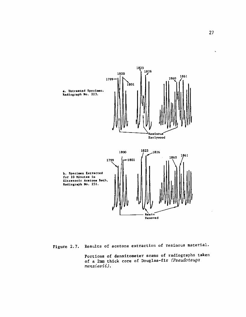
Occasionally specimens will contain dense pockets of resinous material. The resin tends to fill the cell lumens in the earlywood tissues and drastically reduces radiographic contrast in the areas affected, sometimes to the point that it is nearly impossible to distinguish earlywood from latewood on the radiograph. This situation can be partially alleviated by placing the specimens in an ultrasonic bath of acetone or toluene-ethanol mix for about ten minutes. This process does not completely remove the resinous material from the specimen, but enough is removed from the earlywood tissues so that radiographic contrast is sufficient to distinguish the ring boundaries. As can be

26

seen from Figure 2.7, the radiographic density of the latewood tissue is relatively unaffected by the process, probably because it contains very little resin due to the small lumen size of latewood cells. Longer sonication with successive changes of solvent removes more of the resin, but causes excessive softening of the glue used in the mount. It is planned to experiment with other types of glue in the future.

27

a. Untreated Specimen. Radiograph No. 223.

1800

Hesinous'Earlywood

1861

b. Specimen Extracted for 10 Minutes in Ultrasonic Acetone Bath, Radiograph No. 251.

R e s i nRemoved

Figure 2.7. Results of acetone extraction of resinous material.

Portions of densitometer scans of radiographs taken of a 2mm thick core of Douglas—fir (Pseudotsuga menziesii).

CHAPTER 3

RADIOGRAPHY OF CORES

General Methods in UseTwo general schemes of radiography of increment

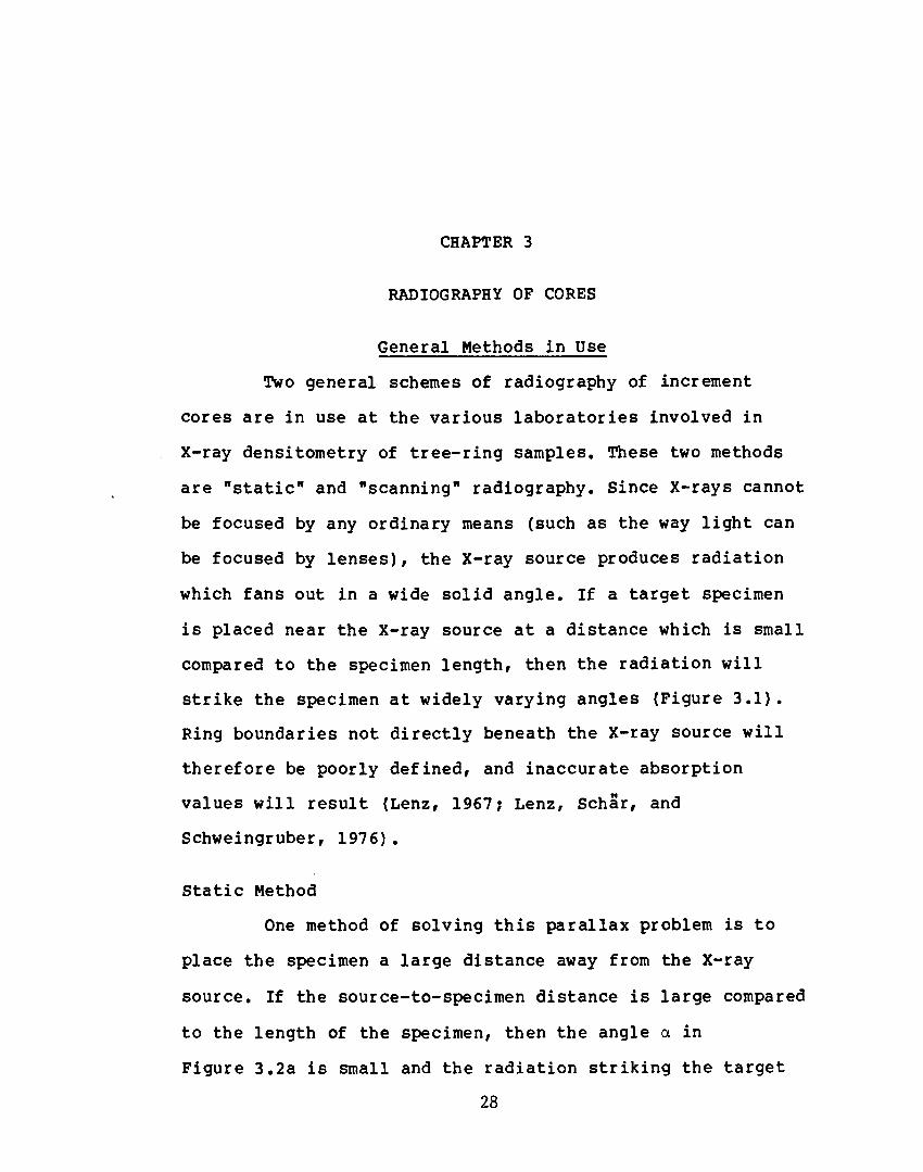
cores are in use at the various laboratories involved in X-ray densitometry of tree-ring samples. These two methods are "static" and "scanning" radiography. Since X-rays cannot be focused by any ordinary means (such as the way light can be focused by lenses), the X-ray source produces radiation which fans out in a wide solid angle. If a target specimen is placed near the X-ray source at a distance which is small compared to the specimen length, then the radiation will strike the specimen at widely varying angles (Figure 3.1). Ring boundaries not directly beneath the X-ray source will therefore be poorly defined, and inaccurate absorption values will result (Lenz, 1967 ? Lenz, Schar, and Schweingruber, 1976).

Static MethodOne method of solving this parallax problem is to

place the specimen a large distance away from the X-ray source. If the source-to-specimen distance is large compared to the length of the specimen, then the angle a in Figure 3.2a is small and the radiation striking the target

28

29

X-ray Source

t=Thickness ofSpecimenWoodSpecimen

Film

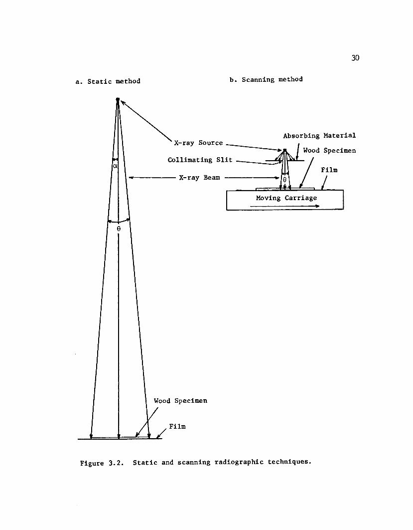
Figure 3.1. Geometric relationship of X-ray source to target.

6 = width of "blur" = t tan a . Note that the width of the "blur" increases as a increases.

30

a. Static method b. Scanning method

Absorbing MaterialX-ray Source

Wood SpecimenCollimating Slit

FilmX-ray Beam

Wood Specimen

Film

Moving Carriage

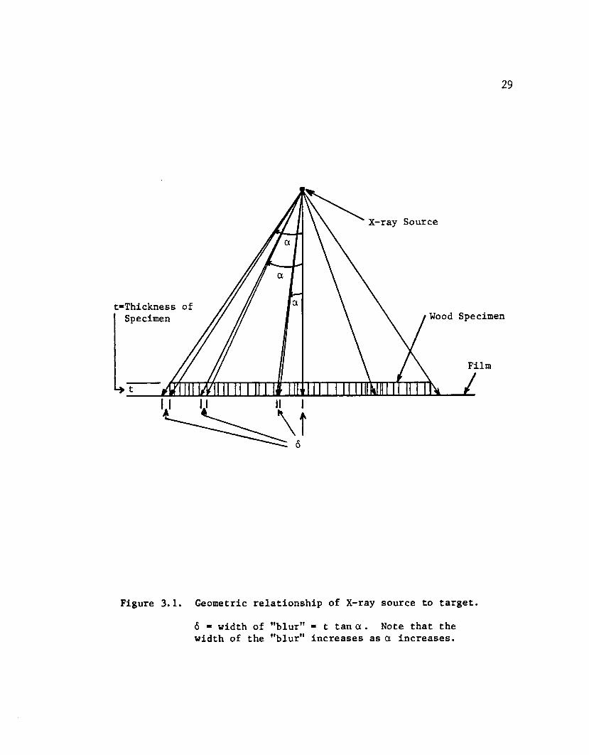
Figure 3.2. Static and scanning radiographic techniques.

31is nearly parallel to the beam axis. This method requires a large work space for exposing the film. In order for the radiation striking a 40 cm specimen to be parallel to within 1° r the specimen must be located about 23 meters from the X-ray source. For safety reasons this entire space must be shielded with lead, concrete, or other suitable material, making the space and shielding requirements for this method rather inconvenient.

At this distance absorption of X-rays by the large air space between target and source becomes very significant (Fletcher and Hughes, 1970, p. 44), especially for the longer wave-length or "soft" X-rays. This air filtering effect necessitates a long exposure time and causes an undesirable shift towards the shorter wave-length or "hard" portion of the spectrum. Another problem is that the radiation intensity may not be uniform over the entire irradiated area, resulting in non-uniform X-ray dosage of the target.

If the cores are of much shorter length or are cut into short pieces, then much less distance is required. It is not uncommon for cores collected by this laboratory to exceed 40 cm in length, and for various reasons it is undesirable to cut them into shorter lengths, making this method of X-ray exposure impractical.

32Scanning Method

Another technique is the scanning method of X-radiography (Echols 1970, Parker and Meleskie 1970) • In this approach a narrow beam or "curtain" of nearly parallel X-rays is produced by means of a collimating slit and the film and specimen are slowly passed through the beam (Figure 3.2b). With this arrangement nearly any desired degree of parallelism of the X-ray beam can be produced, the source-to-target distance can be kept quite small regardless of the length of the specimen, and the entire apparatus may easily be housed in a reasonably small cabinet. This method is used at the University of Arizona Tree-Ring Lab.

Comparison of Scanning and Static MethodsThe static or still method of radiography is much

the simpler of the two. While it requires a large shielded working area, there is no need for machinery to move the film. Because the film does not move, any variation in X-ray intensity during the exposure is unimportant, and there are no problems arising from the vibration of moving parts. If the required exposure time is longer than the maximum duty cycle of the X-ray source, another exposure may be made without moving the target or film as soon as the source is ready again.

33

The scanning method is more convenient, but requires more sophisticated equipment and control, in order to achieve a uniform X-ray exposure throughout the length of the scan it is vital that the X-ray tube output remain constant and that the film scanning speed also remain constant. These problems will be discussed further in the next section.

Scanning Method

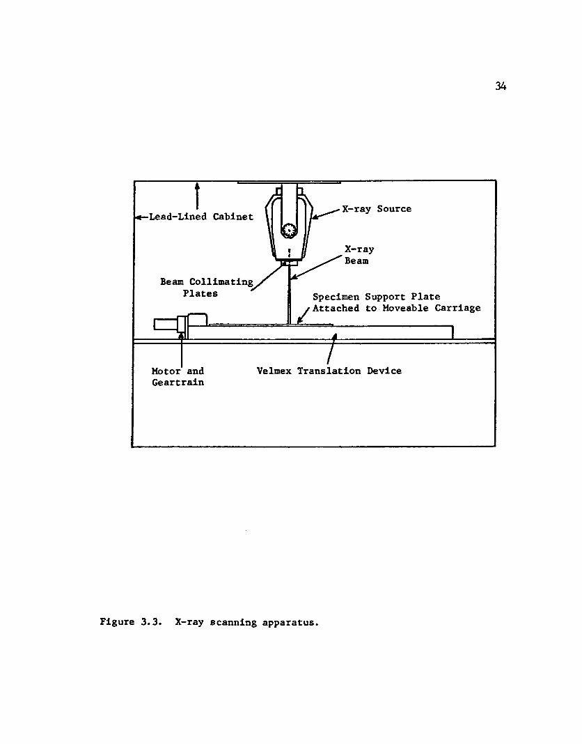
EquipmentThe scanning X-ray apparatus at this laboratory is

enclosed in a lead-lined cabinet approximately two meters wide by two meters tall by one meter deep (Figure 3.3). The film traversing mechanism is a Velmex 64000 series "Onislide" lead-screw translation device. A lead-screw or ■power screw" is a device used to change angular motion into linear motion (Shigley 1963). The wood specimen is placed directly on top of the film on a 60 cm polished aluminum plate attached to the lead-screw carriage (Figure 3.4). This device rests on a platform about 1.1 meters above the floor of the cabinet. The radiation source is an oil-cooled Picker Industrial "Hotshot" 110 kv portable X-ray unit suspended from the roof of the cabinet. The unit incorporates a T40-36 X-ray tube with a 0.5 mm focal spot behind a 0.25 mm beryllium window. Current and voltage are continuously

34

X-ray SourceLead-Lined Cabinet

X-rayBeam

Beam CollimatingPlates Specimen Support Plate

Attached to Moveable Carriage

Velmex Translation DeviceMotor and Geartrain

Figure 3.3. X-ray scanning apparatus.

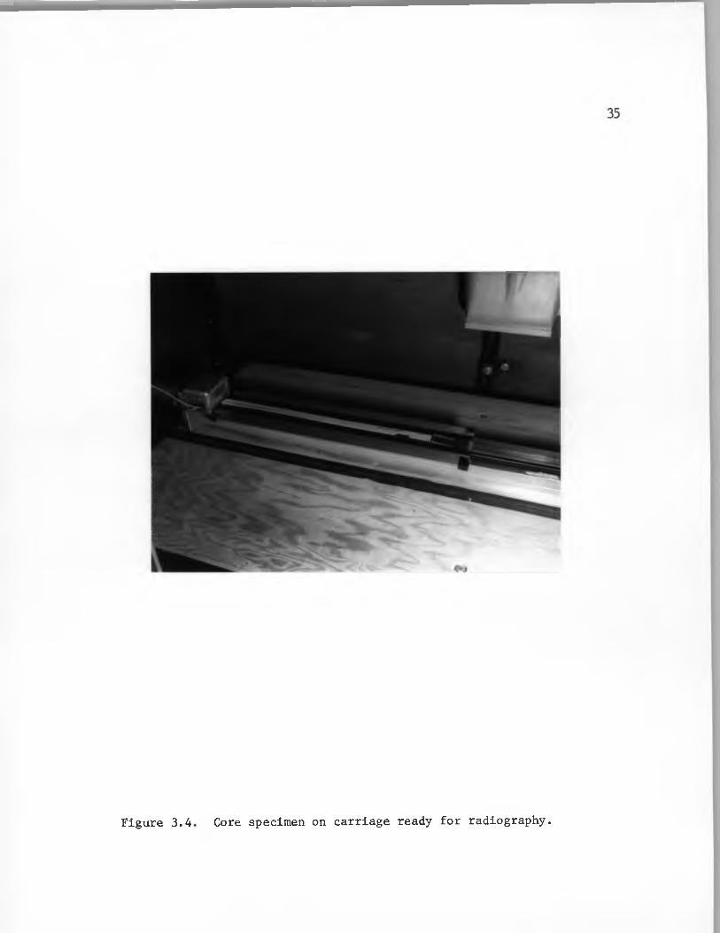
Figure 3.4 Core specimen on carriage ready for radiography.

variable from zero to ten milliamperes and from zero to 110 kilovolts, respectively.

The collimating slit is made of two lead plates separated by 0.7 mm and placed 56 mm below the X-ray focal spot. This configuration produces a maximum beam spread of about 1.25° (Figure 3.5). The degree of collimation is equivalent to that produced by a source-to-specimen distance of 18 meters for a 40 cm specimen in the static technique.The source-to-specimen distance is typically 37 cm, and specimens up to 90 cm in length can be easily handled.

Uniformity of X-ray DosageIn order to attribute the observed variations in

film darkening solely to variations in density of the wood specimen it is essential that the specimen be given a uniform dose of radiation all along its length.

Film Carriage Speed Control. The Velmex lead-screw device for moving the film provides a very stable speed control, regardless of any change in any load or line voltage during the run. However, a very slight increase and decrease in speed occurs at each revolution of the screw. If the collimating slit-to-film distance is very small (15 mm or so), so that the length of the portion of the film which is exposed to the X-ray beam at any instant is of the same order as the pitch of the threads on the lead-screw

36

37

X-ray Source 0.5mm Focal Spot

Lead Collimating / Plates

0.7mm Slit

X-ray Beam

Scale X 2

Figure 3.5. X-ray beam collimation

38(2.5 mm), then the speed variations become apparent as a series of light and dark bands across the radiograph, spaced at 2.5 mm intervals. At a greater siit-to-film distance, the X-ray beam is much wider than the pitch of the screw threads, and this effect is not noticeable, since the individual variations are "smoothed" over a greater length of film.

Regulation of X-ray Tube Output. A similar problem exists with regulation of the X-ray tube output. A Sola 750 watt constant voltage transformer provides regulation of the line current to the X-ray control unit. In addition, the current and voltage meters on the control unit are carefully monitored during each scan, and if the variation exceeds the acceptable limits the run is aborted and another scan is done on the specimen using fresh film. The high-voltage current produced in the X-ray head is not rectified before it is sent to the X-ray tube. The secondary transformer leads are connected directly to the anode and cathode of the X-ray tube. This unrectified alternating current causes the X-ray tube to emit pulses of X-rays at the frequency of the line current, 60 Hz. If the slit-to-film distance is small and the film is scanned at a high speed (greater than about 15 mm/sec. or so) such that each portion of the film experiences only a few pulses of radiation, a series of very fine closely spaced dark lines will appear across the

39

fine closely spaced dark lines will appear across the radiograph. At a slower scan speed and a larger siit-to-film distance this effect is not observed. The angle of collimation of the X-ray beam is the same regardless of the distance from the slit, so no loss of resolution is suffered by increasing the distance. A scan speed of 5.5 mm/sec. at a 32 cm slit-to-film distance produces good quality radiographs. Loss of X-ray beam power due to air absorption and lateral beam spread at this distance is minor, allowing most exposures to be made within the 5-minute maximum duty cycle of the X-ray source.

Film and Exposure

FilmExposures are made with the specimen in direct

contact with the X-ray film. The film used is Kodak Industrex Type M film, an extra-fine grain industrial X-ray film with high contrast. Type M double-emulsion film is available in 35 mm format in 200 ft rolls, which is ideally suited to the scanning method of radiography of increment cores. The film is manually processed on spiral stainless-steel reels using Kodak Liquid X-ray Developer.

Kodak Industrex Type R single emulsion film is an ultra-fine grain X-ray film which should be capable of producing even higher resolution radiographs, but has not

40

been used here because it is not available in 35 mm format in small lots. A small quantity of this type film in 13 cm by 18 cm sheets has recently been purchased for experimental purposes.

Exposure CriteriaIn order to produce accurate wood density

measurements from the radiographs it is essential that the degree of film darkening be related to the specimen density in a reasonably simple and predictable manner. X-ray absorption by wood and the resultant film darkening is not a linear function of wood density, but may be approximately described by the Lambert-Beer Law,

I - lo •4 “

where I is the intensity of transmitted radiation of a particular wavelength, I is the intensity of the incident X-ray beam, k is the absorption coefficient for a particular substance at a single wavelength, x is the sample thickness, and c is the concentration of the substance, or density (Daniels and Alberty 1975, p. 512). Since the radiation produced by the X-ray tube is not of a single wavelength but consists of a broad spectrum of wavelengths, and because the absorption coefficient k is not readily available for individual wood species, the Lambert-Beer Law may not be

41

directly used to compute wood densities, but does illustrate the general relationship of absorption to density. The actual method used to compute wood density from film darkening will be discussed in the next chapter.

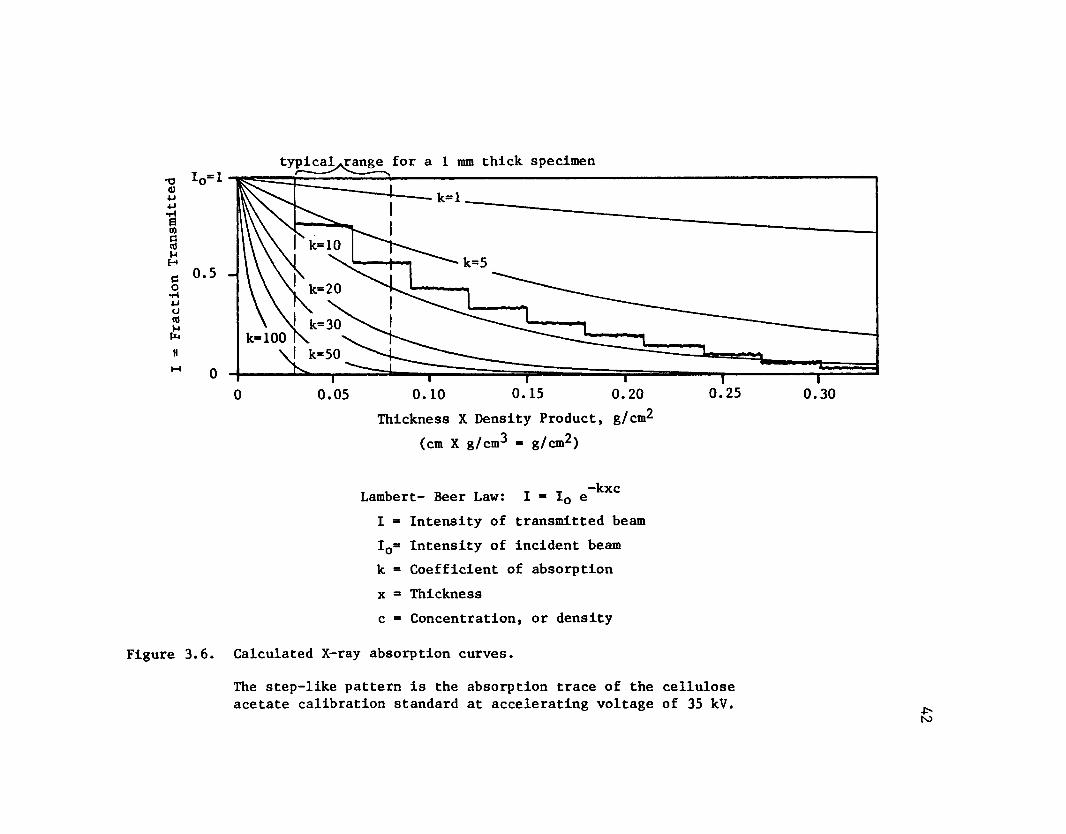
According to the Eastman Kodak manual Radiography in Modern Industry (1969) and to Polge and Nicholls (197 2) X-rays of lower energy levels (long-wave or "soft" radiation) provide more radiographic contrast but a less nearly linear relationship of absorption to specimen density than X-rays of higher energy levels (short-wave or "hard" radiation). Figure 3.6 shows calculated absorption coefficients throughout the range of density-thickness products normally encountered in specimens up to 3 mm thick. The absorption coefficient k decreases as the wavelength decreases (Chemical Rubber Publishing Co., Handbook of Chemistry and Physics, 43rd Ed. 1961-62, pp. 2718-2723), and thus short-wave radiation has greater penetrating power (less absorption) than long-wave radiation. When the wavelength (and the absorption coefficient) is small, the exponential absorption curve approximates a linear function (Polge 1966, p. 299), but radiographic contrast is low (Polge 1966, p. 83), since the difference in the fraction of radiation transmitted through the specimen is quite small between the density-thickness extremes encountered. For example, for a specimen thickness of one millimeter (0.1 cm)

Frac

tion

Tra

nsmi

tted

typlcal^range for a 1 mm thick specimen

k=100

Thickness X Density Product, g/cm^(cm X g/cm^ - g/cm^)

“IcxcLambert- Beer Law: I = I0 eI = Intensity of transmitted beam I0= Intensity of incident beam k = Coefficient of absorption x = Thicknessc = Concentration, or density

Figure 3.6. Calculated X-ray absorption curves.

The step-like pattern is the absorption trace of the cellulose acetate calibration standard at accelerating voltage of 35 kV.

43

and a minimum earlywood to maximum latewood density range of 0.3 g/cm^ to 0.8 g/cm^, reasonable values for many wood specimens, the density-thickness product range is 0.03 g/cm2 to 0.08 g/cm2, or 0.05 g/cm2. The curve for coefficient k = 1 is quite nearly linear in this range, but the difference in the transmitted radiation fraction is very small (.97 to .90). For the curve k = 30 much more contrast is available, but the curve is decidedly non-linear. The curve k = 10 provides both reasonable linearity and fairly strong contrast.

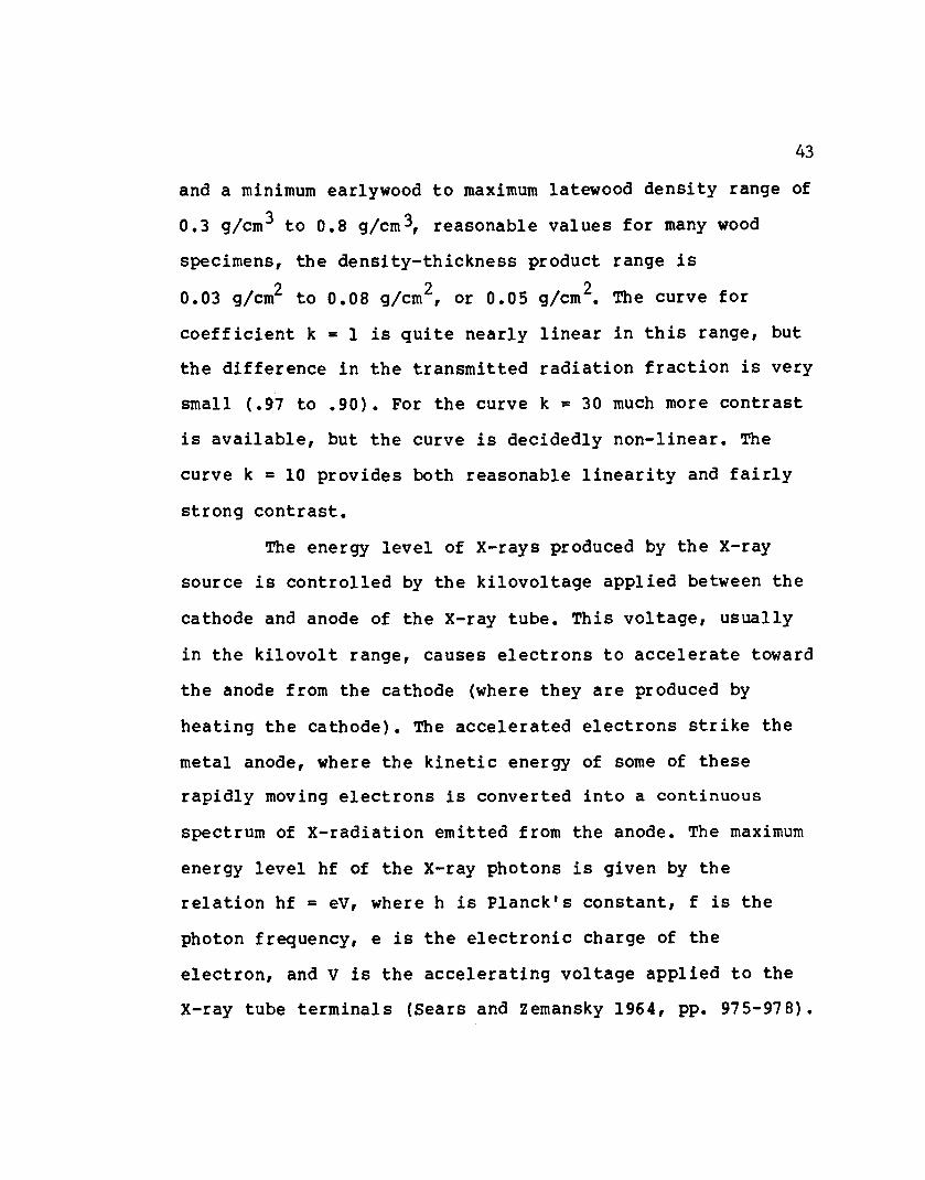
The energy level of X-rays produced by the X-ray source is controlled by the kilovoltage applied between the cathode and anode of the X-ray tube. This voltage, usually in the kilovolt range, causes electrons to accelerate toward the anode from the cathode (where they are produced by heating the cathode). The accelerated electrons strike the metal anode, where the kinetic energy of some of these rapidly moving electrons is converted into a c o n t i n u o u s spectrum of X-radiation emitted from the anode. The maximum energy level hf of the X-ray photons is given by the relation hf = eV, where h is Planck's constant, f is the photon frequency, e is the electronic charge of the electron, and V is the accelerating voltage applied to the X-ray tube terminals (Sears and Zemansky 1964, pp. 975-978).

In choosing a working kilovoltage level, it is desirable that the exposed radiograph provide enough optical contrast to be accurately measured by a scanning microdensitometer, and that the relationship between film darkening and specimen density be sufficiently close to linear that reliable estimates of wood density may be made. Obviously, no single kilovoltage level will provide maximum contrast and perfect linearity, so a workable compromise must be sought suited to the particular type of film, X-ray tube, and optical densitometer used.

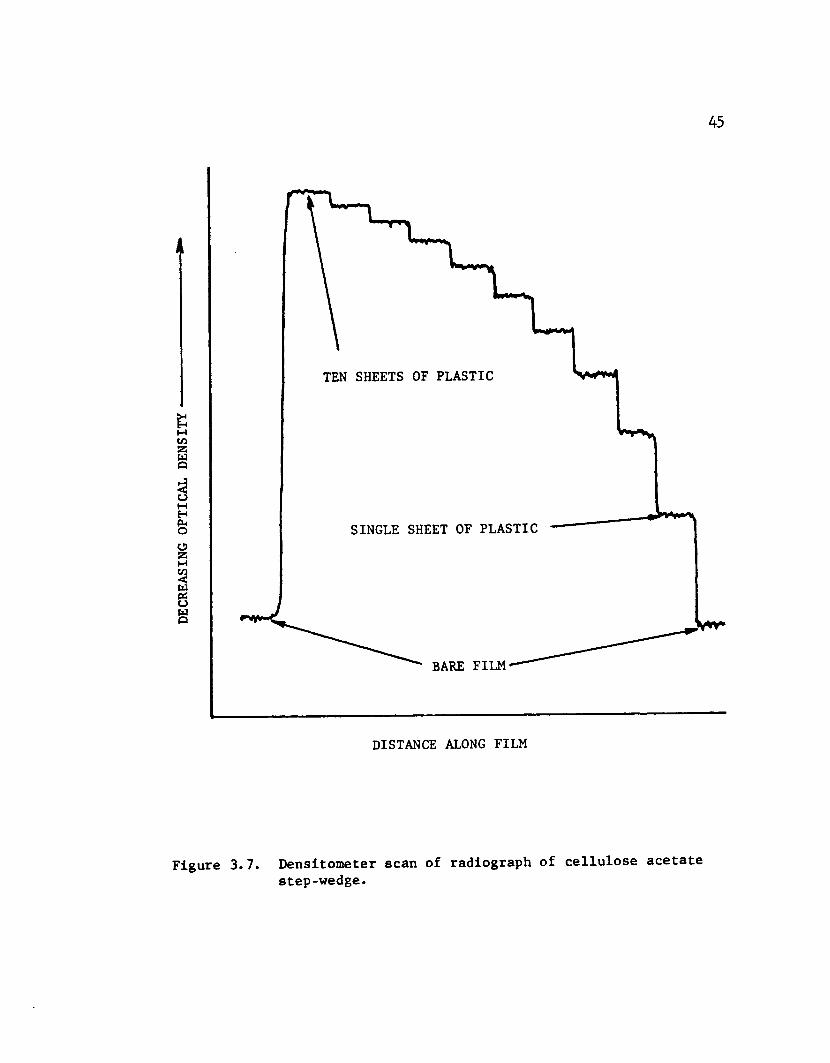
It has been found by experimentation that a peak energy level of 35 kv meets these requirements fairly well. Figure 3.7 shows a densitometric scan of a radiograph taken at 35 kv of a ten-step cellulose acetate step-wedge calibration standard which adequately covers the entire range of wood densities encountered. Tube current is 5 milliamperes at a scan speed of 5.5 mm/sec. The logarithmic relationship of film darkening to specimen density is apparent in this radiograph, but enough radiographic contrast is present to allow accurate optical density measurements to be made throughout the density range. The measurements of film darkening may then be transformed into accurate wood density estimates using the technique described in Chapter 4. Figure 3.6 also shows an estimate of the radiation fraction absorbed by the plastic

44

DECR

EASI

NG O

PTIC

AL D

ENSI

TY

45

DISTANCE ALONG FILM

Figure 3.7. Densitometer scan of radiograph of cellulose acetate step-wedge.

calibration wedge. Apparently the 35 kv radiation spectrum behaves as if its absorption coefficient (for cellulose acetate) were close to k = 9.

Exposure ProcedureThe X-ray exposures are made under darkroom

conditions. Safelights of 15 watts with Kodak No. 6B Wratten filters are used to provide enough illumination to position the film and specimen for the exposure. Film and specimen are both taped to the specimen plate to avoid any possible shifting and consequent blurring of the radiograph during the run. The specimen is placed directly in contact with the bare film, since light-tight X-ray exposure holders do not appear to be suitable for the low X-ray dosages which are used. Kodak exposure holders were experimented with, but it was found that the variations in density of the paper and cardboard fibers of the holders were significant compared with the density variations of the thin wood specimens. Essentially the same results were obtained by Polge (1965, p. 10). The calibration step-wedge is placed on the film near the bark end of the core. The films are numbered sequentially and are identified by placing small lead numerals on the core mount before exposure.

46

CHAPTER 4

OPTICAL DENSITOMETRY

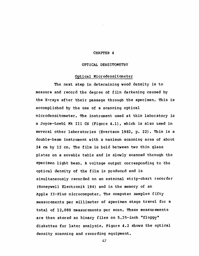
Optical Microdensitometer The next step in determining wood density is to

measure and record the degree of film darkening caused by the X-rays after their passage through the specimen. This is accomplished by the use of a scanning optical microdensitometer. The instrument used at this laboratory is a Joyce-Loebl Mk III CS (Figure 4.1), which is also used in several other laboratories (Evertson 1982, p. 22). This is a double-beam instrument with a maximum scanning area of about 24 cm by 12 cm. The film is held between two thin glass plates on a movable table and is slowly scanned through the specimen light beam. A voltage output corresponding to the optical density of the film is produced and is simultaneously recorded on an external strip-chart recorder (Honeywell Electronik 194) and in the memory of an Apple II-Plus microcomputer. The computer samples fifty measurements per millimeter of specimen stage travel for a total of 12,000 measurements per scan. These measurements are then stored as binary files on 5.25-inch "floppy" diskettes for later analysis. Figure 4.2 shows the optical density scanning and recording equipment.

47

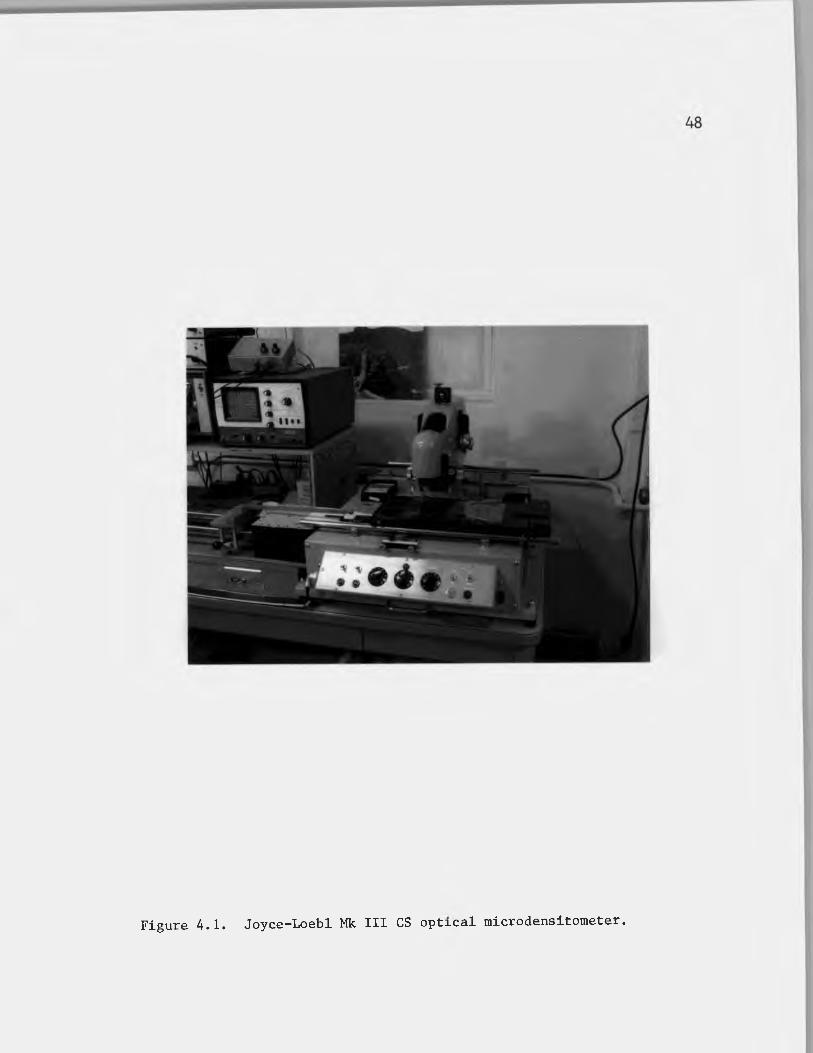
Figure 4.1, Joyce-Loebl Mk. XXX CS optxcsX iniGirodonsitoniGtsir.

49

Figure 4.2. Optical densitometry measuring and recording system.

50

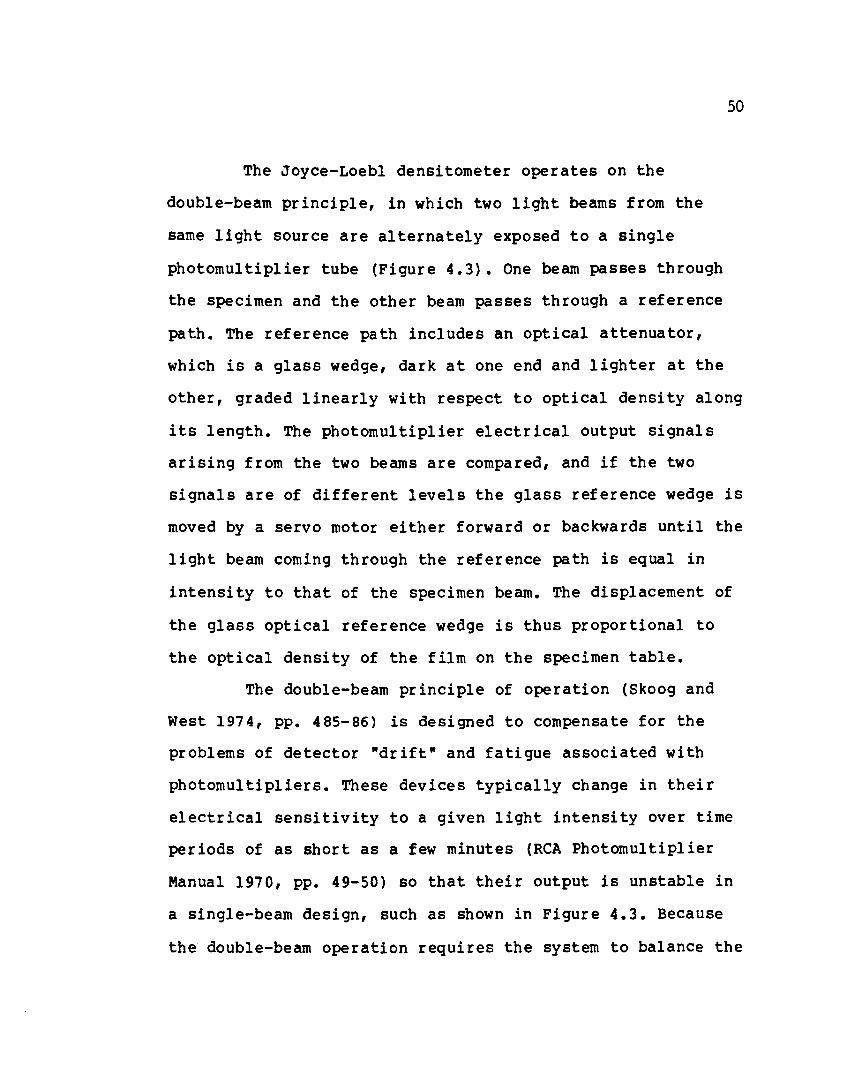
The Joyce-Loebl densitometer operates on the double-beam principle, in which two light beams from the same light source are alternately exposed to a single photomultiplier tube (Figure 4.3). One beam passes through the specimen and the other beam passes through a reference path. The reference path includes an optical attenuator, which is a glass wedge, dark at one end and lighter at the other, graded linearly with respect to optical density along its length. The photomultiplier electrical output signals arising from the two beams are compared, and if the two signals are of different levels the glass reference wedge is moved by a servo motor either forward or backwards until the light beam coming through the reference path is equal in intensity to that of the specimen beam. The displacement of the glass optical reference wedge is thus proportional to the optical density of the film on the specimen table.

The double-beam principle of operation (Skoog and West 1974, pp. 485-86) is designed to compensate for the problems of detector "drift" and fatigue associated with photomultipliers. These devices typically change in their electrical sensitivity to a given light intensity over time periods of as short as a few minutes (RCA Photomultiplier Manual 1970, pp. 49-50) so that their output is unstable in a single-beam design, such as shown in Figure 4.3. Because the double-beam operation requires the system to balance the

51

Light Path

Condensing ' Lens '

Objective ApertureLens

PhotodetectorLight SpecimenSource/ Chopper

Wheel (Shutter)

SpecimenLightPath

Optical wedgeServo

System

Reflecting Prisms

AnalogPick-up Device

Output

ReferenceLight Path

Figure 4.3. Schematic diagram, single-beam and double-beam optical densitometer principles.

The single-beam principle is illustrated in the upper drawing; the double-beam principle is illustrated in the lower drawing.

52

amount of light coming through the reference path until it is equal to that of the specimen path, problems of detector drift and fatigue, detector non-linear response, and changes in the intensity of the light source are minimized. However, this compensation is obtained at the expense of reduced response speed. Time must be allowed for the servo-balancing system to move the reference wedge into an equilibrium position. Because a single scan of a tree-ring series often consists of over a hundred annual rings, at each boundary of which a rapid optical density change occurs, the scan speed must be around one millimeter per second or less in order to obtain reproducible and accurate results. Double-beam instruments are considerably more complex than single-beam densitometers and as a result are much more expensive and more difficult to maintain.

Recording SystemThe Joyce-Loebl instrument was originally designed

and equipped with its own recording table, located at the rear of the unit below the optical reference wedge, mechanically linked to the specimen table and moving in opposition to it. A pen attached to the moving carriage of the optical reference wedge recorded the varying optical density of the specimen on graph paper clipped to the recording table.

This recording system is not used in our application. In many of the tree-ring series studied the width of the rings is so narrow that they cannot be resolved on the paper recording if the recording table is moved at a 1:1 ratio with the specimen table. The recording table can be moved at several higher ratios (up to 200:1), but only at the expense of proportionally reduced scan lengths on the specimen. Since continuous scans of maximum length are highly desirable an external recording system is used.

A factory-fitted analog output device provides a voltage signal proportional to the position of the optical wedge. This voltage is recorded in expanded form on an external strip-chart recorder. The analog device is a free-turning zero-to-100-ohm precision potentiometer actuated by the chain drive system which moves the optical wedge. The potentiometer is energized by a 2.00 volt reference voltage from a Hewlett-Packard 6204B DC power supply. The potentiometer acts as a voltage divider for the 2 volt reference voltage. As the position of the wedge changes, the resistance of the potentiometer changes proportionally and a corresponding voltage between zero and two volts appears at the center terminal of the potent!ometer.

53

54

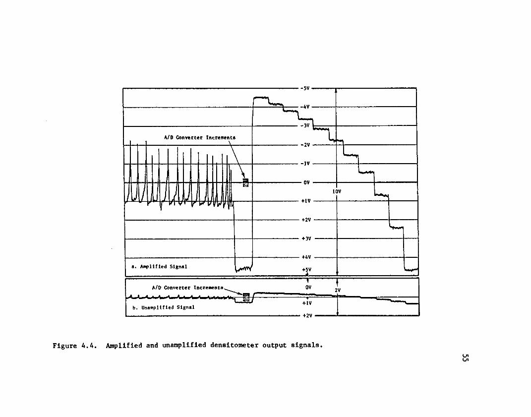
Signal AmplificationThe difference in densitometer output voltage

corresponding to earlywood minimum density and latewood peak density is typically on the order of 0.2 volt, or 200 millivolts (Figure 4.4b). The analog-to-digital converter used with the Apple computer (Mountain Hardware A/D + D/A) is an 8-bit converter which plugs into one of the peripheral slots at the rear of the Apple. It provides an 8-bit digital output signal to the Apple corresponding to a 10-volt input voltage spread ranging from -5V to +5V. In other words, the 8-bit output means there are 256 possible digital numbers (0-255) which may represent the input signal. An input of -5V or less produces the number zero, a zero analog input voltage produces 128, and a +5V or higher analog voltage is digital 255. Thus the resolution of the A/D converter is such that the analog input voltage must change by 39 millivolts to produce one incremental change in the output digital number. For an input signal which varies by only 200mV, only about 5 or 6 different possible numbers corresponding to the input voltage would be read by the Apple.

To resolve this difficulty the densitometer output signal is amplified so that the entire voltage spread from that corresponding to the bare film level to the densest step of the calibration wedge (discussed in Chapter 4) is

A/D Converter Increments

a. Amplified Signal

A/D Converter Increments

b. Unamplified Signal

Figure 4.4. Amplified and unamplified densitometer output signals.inin

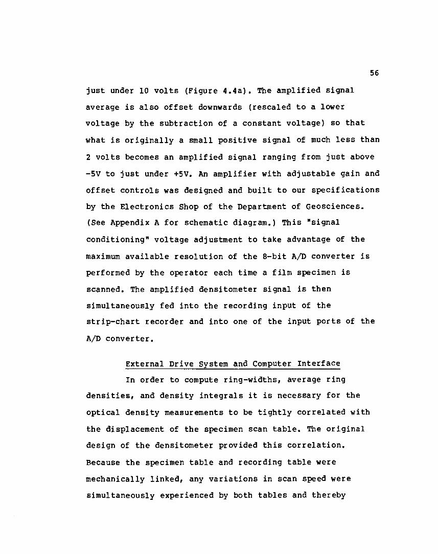
56

just under 10 volts (Figure 4.4a). The amplified signal average is also offset downwards (rescaled to a lower voltage by the subtraction of a constant voltage) so that what is originally a small positive signal of much less than 2 volts becomes an amplified signal ranging from just above -5V to just under +5V. An amplifier with adjustable gain and offset controls was designed and built to our specifications by the Electronics Shop of the Department of Geosciences. (See Appendix A for schematic diagram.) This "signal conditioning" voltage adjustment to take advantage of the maximum available resolution of the 8-bit A/D converter is performed by the operator each time a film specimen is scanned. The amplified densitometer signal is then simultaneously fed into the recording input of the strip-chart recorder and into one of the input ports of the A/D converter.

External Drive System and Computer InterfaceIn order to compute ring-widths, average ring

densities, and density integrals it is necessary for the optical density measurements to be tightly correlated with the displacement of the specimen scan table. The original design of the densitometer provided this correlation.Because the specimen table and recording table were mechanically linked, any variations in scan speed were simultaneously experienced by both tables and thereby

57

compensated. Measurements between density variations on the paper recording would faithfully reproduce the distances between those same variations on the specimen. To produce the same association of optical density measurements with specimen location on an external chart recorder or computer, it is necessary for the specimen table motion to be very stable and constant. At the slowest whole-table scan speed available with the internal drive mechanism of this model densitometer the scan speed is extremely unstable and shows very poor reproducibility. Moreover, the slowest whole-table scan speed is not slow enough to provide reliably accurate measurements of the rapidly changing optical densities along the scan.

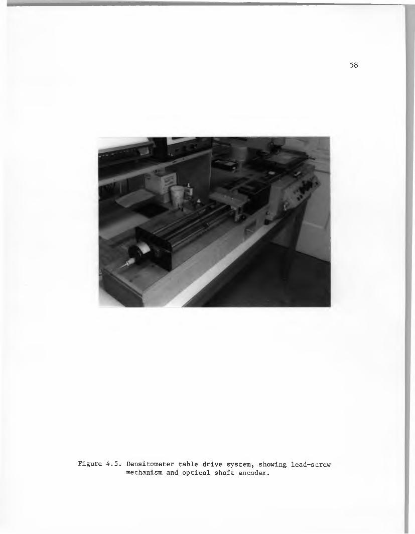
To overcome this problem an external specimen table drive system is employed (Figure 4.5). The drive system consists basically of a precision lead-screw with a pitch of one turn per millimeter coupled by a half-nut linkage assembly to a rider platform which is in turn linked by a connecting rod to the specimen table. The specimen table is uncoupled from the internal drive system of the densitometer. The lead-screw is driven at 36 rpm by a small electric gearmotor. This arrangement moves the specimen table at 0.6 mm/sec. It is planned to replace this single-speed motor with a variable-speed reversible

58

Figure 4.5. Densitometer table drive system, showing lead-screw mechanism and optical shaft encoder.

59gearmotor or stepper motor in the near future. A quick- disconnect mechanism on the half-nut linkage allows the table to be rapidly positioned by hand for setting up the run.

The other end of the lead-screw is fitted with an optical incremental shaft encoder (Data Tech, Opticon Series Model OC25), which provides opto-electronic sensing of the lead-screw's angular motion. The shaft encoder produces 500 low-voltage output pulses per revolution, or one pulse per 0.72° of shaft rotation. Since the pitch of the precision lead-screw is one millimeter per turn, the shaft encoder output is thus one pulse for every 0.002 mm of specimen table travel.

This position signal is fed into a simple digital logic control circuit which divides the input frequency by ten, producing one output timing pulse per 0.02 mm of specimen displacement. The timing signal is routed to one of the push-button input pins of the Game In/Out connector on the Apple II main circuit board, and is used as a triggering signal for the Apple to read and store the current data at the A/D converter. The digital logic circuit was designed by David Steinke of the Department of Geosciences Electronics Shop. (See Appendix A for schematic diagram.)

60

Computer SoftwareThe Apple II computer is controlled by a

BASIC-language program called TRIGGER. (See Appendix B for program listing.) After initialization the program monitors the status of the push-button input port. When a low input status signals the beginning of an input timing pulse, the program reads the current value of the A/D converter, stores it in memorey, and returns to monitor the push-button status for the next pulse. This process is repeated until a specified number of readings have been performed - usually 12,000, corresponding to the full 24 centimeters of specimen table scan.

Since the memory size of the Apple II computer is somewhat limited, numbers corresponding to the displacement position of the scan table are not recorded along with the optical density measurements. These measurements are simply stored in sequential memory locations, one 8-bit single-byte measurement occupying one memory address. The contents of the block of memory is then stored as a binary file on a 5.25-inch diskette. Subsequent programs compute the desired position and width measurements from the position-in-file, each file position corresponding to 0.02 mm displacement along the scan.

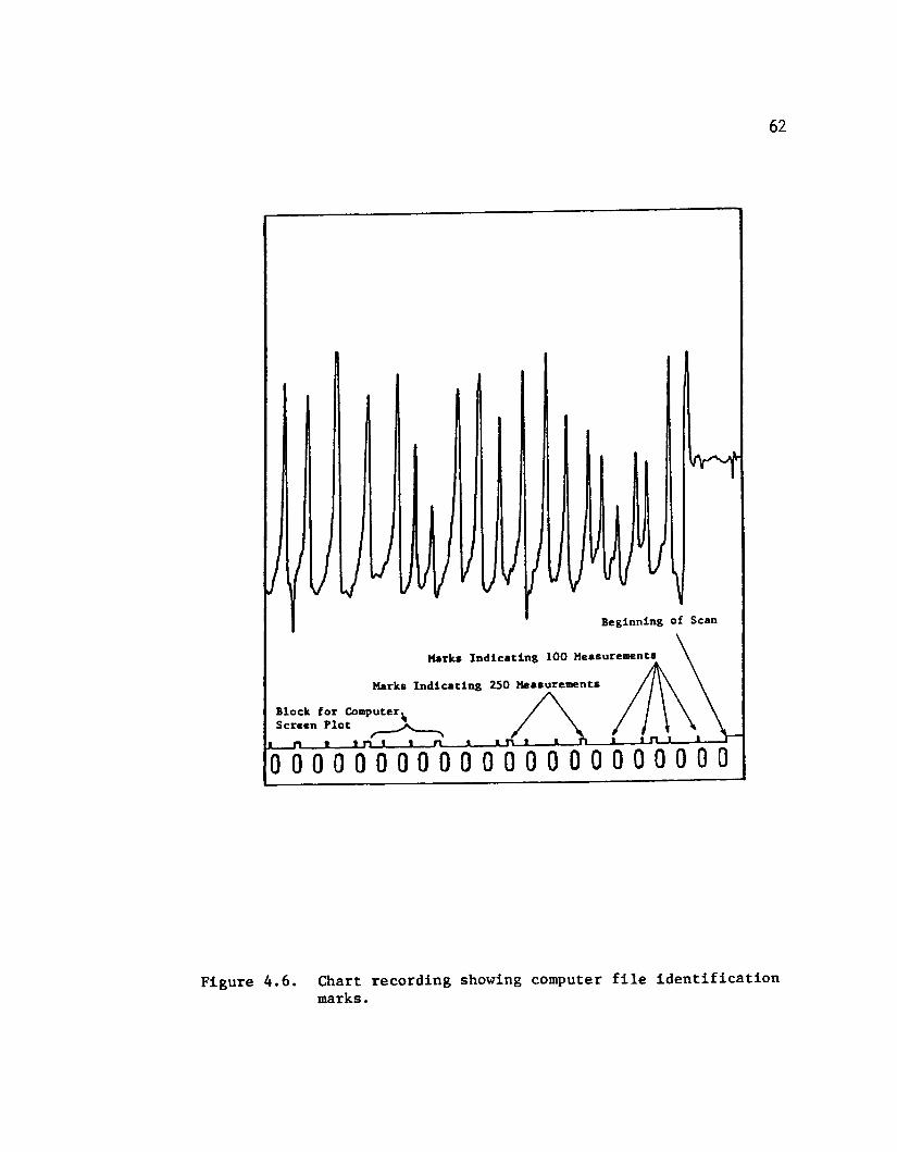
The digital logic control circuit also provides a signal for marking the edge of the paper chart recording

61

(Figure 4.6) via the event pen on the Honeywell chart recorder. The event pen is activated by 110V AC line current. The control circuit operates an optically-coupled TRIAC device to switch the line current on and off to the event pen. At each 100 control pulses (5V DC) sent to trigger the Apple, a short (0.1 sec.) pulse of 110V line current is sent to activate the event pen on the chart recorder. In this way a series of "blips" along the margin of the chart recording marks the position of every 100th measurement in the corresponding computer file. In addition, a longer pulse (0.5 sec.) of line current is switched to the event pen at every 250 measurements. This longer "blip" marks the boundaries of each block of measurements which is later displayed on the Apple high-resolution graphics screen by a subsequent program called BOUNDARY CHECK, described in the next chapter.

Current System Limitations

Scan Length and Film PositioningSome major problems involved with the use of the

Joyce-Loebl microdensitometer remain unsolved. The maximum scan length of 24 cm is not long enough to accommodate a radiograph of a typical tree-ring radius plus the step-wedge calibration standard. Most radiographs require two or more scans to cover their entire length. This problem is

62

B e g i n n i n g of Scan

Harks I n d i c a t i n g 100 M e a s u r e m e n t s

Marks Indicating 250 MeasurementsB l o c k for Comp u t e rScreen Plot

0 0 0 0 0 0 0 0 0 0 0 0 0 0 0 0 0 0 0 0 0 0

Figure 4.6. Chart recording showing computer file identification marks.

63currently dealt with by a BASIC-language program called MATCH, which matches together two overlapping sets of density measurements and corrects for any electronic or optical drift which may occur when the film is repositioned. This problem adds to the bulkiness of the data storage and to the complexity of the manipulation process. Possible solutions include the design and construction of a longer specimen table to take advantage of the full 45 cm traverse of the precision lead-screw, or the construction of a new densitometer dedicated to this application.

Another problem is the difficulty of positioning the film on the specimen table prior to making a scan. The table and lighting arrangements are such that it is extremely difficult to see the film specimen with any clarity when it is mounted on the specimen table, and much uncertainty is involved concerning the exact location of the line of scan. An image of the film is projected onto the collimating plates of the densitometer, but it is so small and dim even in a darkened room as to be of little or no value in determining the line of scan. A system which could project a larger and much brighter image of a larger portion of the film onto a screen or grid would be very helpful.

Non-rotatable Secondary Apertures.A more serious problem is that the secondary

collimating slits of the densitometer are not rotatable.

64

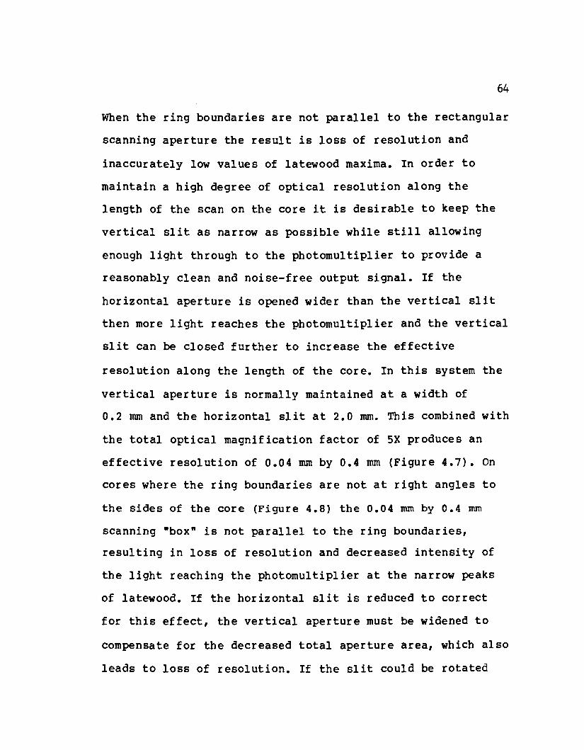
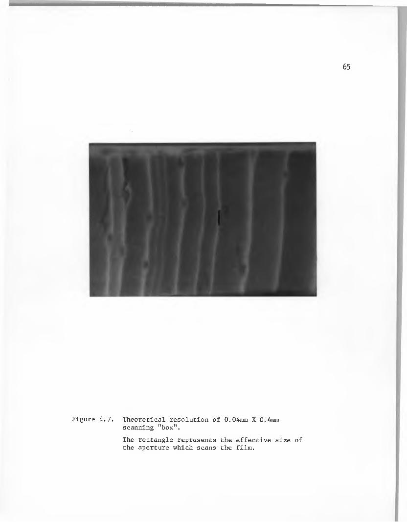
When the ring boundaries are not parallel to the rectangular scanning aperture the result is loss of resolution and inaccurately low values of latewood maxima. In order to maintain a high degree of optical resolution along the length of the scan on the core it is desirable to keep the vertical slit as narrow as possible while still allowing enough light through to the photomultiplier to provide a reasonably clean and noise-free output signal. If the horizontal aperture is opened wider than the vertical slit then more light reaches the photomultiplier and the vertical slit can be closed further to increase the effective resolution along the length of the core. In this system the vertical aperture is normally maintained at a width of 0.2 mm and the horizontal slit at 2.0 mm. This combined with the total optical magnification factor of 5X produces an effective resolution of 0.04 mm by 0.4 mm (Figure 4.7). On cores where the ring boundaries are not at right angles to the sides of the core (Figure 4.8) the 0.04 mm by 0.4 mm scanning "box" is not parallel to the ring boundaries, resulting in loss of resolution and decreased intensity of the light reaching the photomultiplier at the narrow peaks of latewood. If the horizontal slit is reduced to correct for this effect, the vertical aperture must be widened to compensate for the decreased total aperture area, which also leads to loss of resolution. If the slit could be rotated

65

Figure 4.7. Theoretical resolution of 0.04mm X 0.4mm scanning "box".The rectangle represents the effective size of the aperture which scans the film.

66

Figure 4.8. Relationship of scanning "box" to slanted ring boundary.

67during the scan this problem would be alleviated. It is possible to have the Joyce-Loebl machine factory-fitted with a beam-rotation attachment, but this has not been done due to time and cost considerations. Construction of a dedicated instrument would allow the incorporation of a rotatable collimating slit into its design.

Densitometer ResolutionResolution of Narrow Rings. In some cases where the

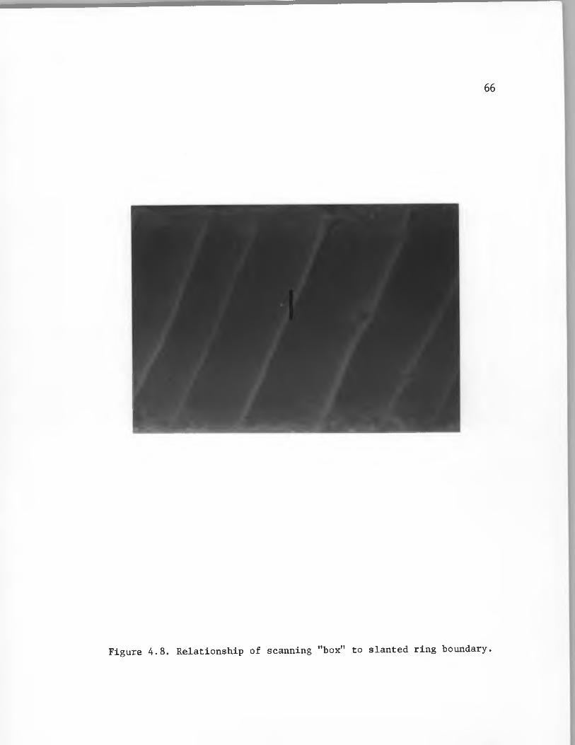
rings are very narrow ( 0.2 mm or so ), but are clearly defined on the radiograph, the standard 0.2 mm X 2.0 mm aperture setting does not provide sufficient resolution to clearly define the ring boundaries. This situation is exacerbated by poorly aligned rings as described in the preceding section. Even though the theoretical effective resolution at this setting is 0.04 mm X 0.4 mm when combined with the 5X magnification factor, it is extremely difficult to achieve this precision in practice owing to the difficulty in seeing the projected image clearly enough to precisely focus it on the aperture screen (Figure 4.9) The narrow ring in the center of the field is about 0.09 mm wide, but is not resolved by the densitometer, even when the vertical and horizontal apertures are set at 0.1 mm and 0.5 mm, giving a theoretical resolution of 0.02 mm X 0.1 mm.

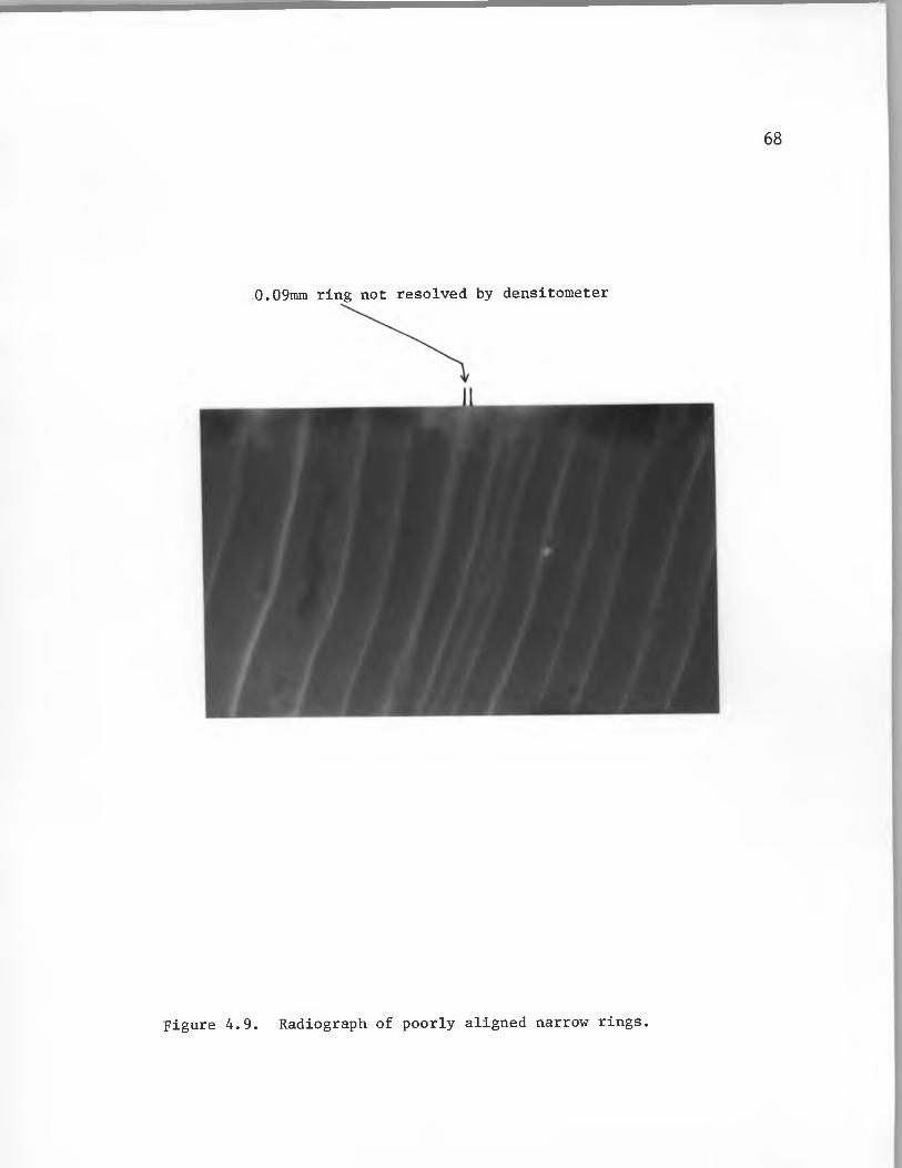
68

0.09mm ring not resolved by densitometer

Figure 4.9. Radiograph of poorly aligned narrow rings.

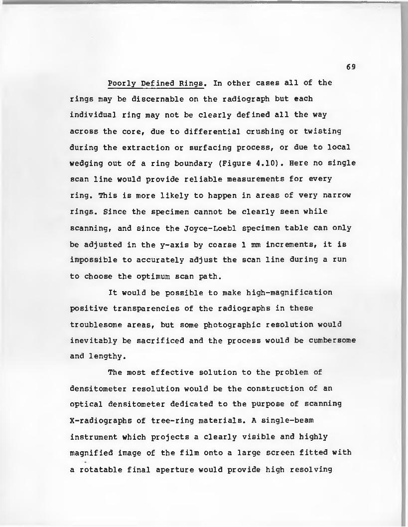
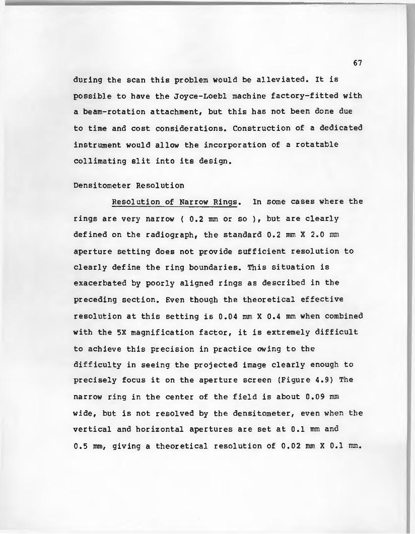
69Poorly Defined Rings. In other cases all of the

rings may be discernable on the radiograph but each individual ring may not be clearly defined all the way across the core, due to differential crushing or twisting during the extraction or surfacing process, or due to local wedging out of a ring boundary (Figure 4.10). Here no single scan line would provide reliable measurements for every ring. This is more likely to happen in areas of very narrow rings. Since the specimen cannot be clearly seen while scanning, and since the Joyce-Loebl specimen table can only be adjusted in the y-axis by coarse 1 mm increments, it is impossible to accurately adjust the scan line during a run to choose the optimum scan path.

It would be possible to make high-magnification positive transparencies of the radiographs in these troublesome areas, but some photographic resolution would inevitably be sacrificed and the process would be cumbersome and lengthy.

The most effective solution to the problem of densitometer resolution would be the construction of an optical densitometer dedicated to the purpose of scanning X-radiographs of tree-ring materials. A single-beam instrument which projects a clearly visible and highly magnified image of the film onto a large screen fitted with a rotatable final aperture would provide high resolving

70

Figure 4.10. Radiograph of slightly damaged rings.

The rings to the left of the crack in the center (dark wedge) do not appear to be continuous in the radiograph, probably due to poor local alignment caused by twisting and crushing during extraction of the core.

power and ease of focusing and would allow the operator to see what is being scanned and to adjust the scan path or aperture angle as necessary.

Other Possible Approaches

Single-beam DensitometerA prototype single-beam instrument using a scanning

film holder of 48 cm traverse was constructed at this laboratory in the spring of 1981. A light source of considerably more power than that used in the Joyce-Loebl instrument was employed to project a magnified image of about 4 cm of the film onto a screen several feet away. The overall magnification factor is about 20X. A collimating slit is installed in the center of the screen. The light passing through this aperture was focused with a Hastings Triplet lens onto the sensitive spot of a low-cost phototransistor, the output of which was fed into the Honeywell chart recorder. Although the phototransistor's response time was rather slow, the apparatus produced excellent results when the film holder was scanned past the light source at a speed of about 0.5 mm/sec. by the Velmex translation device described in Chapter 2. The device gave a very clean output signal with no detectable drift at a resolution of 0.01 mm along the scan. The ability to see a clear image of a large portion of the film being scanned was of great convenience. It would be a relatively simple matter

71

72

to add rotatable slit capability to this design. Stability could be added to the system by regulating the light source output with a supply-voltage control circuit employing feedback from a second optical detector located inside the light source compartment. Replacement of the phototransistor as the primary detector with a temperature-stabilized photodiode detector should greatly increase the response speed, allowing scan speeds of several millimeters per second.

Further development of this device has been postponed following the promising initial results so that efforts could be concentrated on developing the overall X-ray densitometry system, especially the software and interface hardware associated with computerization.

Video Image AnalyzerAnother approach is to use a microcomputer-based

video image analyzer as described by Telewski, Wakefield, and Jaffe (1982) in place of the optical densitometer. The image analyzer uses an Apple 11+ microcomputer, an analytical quality video camera, and a video digitizer. The system was demonstrated by Mr. Telewski to operate satisfactorily on the Apple computer in use at this lab in October, 1982 (Telewski, 1982). This system has the advantage of displaying on a monitor screen a large image of

73

the portion of the radiograph to be scanned. The scan line may then be precisely programmed by the operator.

CHAPTER 5

DATA MANIPULATION AND CALIBRATION

The next step in densitometric analysis is to transform the optical density values to wood density and to edit the large data files of several thousand numbers per core in order to identify annual ring boundaries and to select one value per ring for the various growth characteristics of interest. These characteristics include maximum latewood density, minimum earlywood density, and average density of individual annual growth rings. Several computer programs have been developed for the Apple to facilitate this.

The most critical of these tasks is the identification of annual ring boundaries, for which the judgement of a trained technician is considered to be essential. The technician must be able to differentiate between true ring boundaries and false rings, resin pockets, cracks in the specimen, and occasional anomalies caused by dust particles on the support glass, pieces of sanding grit embedded in the specimen, and scratches in the film emulsion. The technician must also make decisions regarding problems of low radiographic resolution in areas of poor ring geometry or very narrow rings, and must insert proxy

74

75values where rings are locally absent. A program relying heavily on visual interpretation of data plotted on the Apple high-resolution graphics screen is used to allow the technician to review the data and make the final decision on all the selected data points.

Program Calibrate

Cellulose Acetate Calibration StandardThe first data manipulation program provides the

necessary coefficients to later transform the optical density measurements to wood specific gravity estimates.This program is called CALIBRATE. As pointed out in Chapter 3, the relationship of film darkening to wood density is not linear, but logarithmic (Figure 3.8). For this reason a calibration step wedge standard made of one to ten thicknesses of 0.023 mm cellulose acetate is radiographed with every wood specimen. The "areal" density of this plastic step wedge varies by a known amount. Areal density is defined as mass per unit area, or the total mass of absorbing material between the X-ray source and unit area of film. It is not the same as the conventional density of the wood (mass per unit volume, an intrinsic property independent of the amount of material present), but rather it is the product of the wood density times the sample thickness, and is thus an extrinsic property dependent on

76the thickness. It is this areal density of the specimen which determines the proportion of the X-ray beam that will be absorbed by the wood, since the X-rays cannot distinguish between thickness and density. (See the discussion on the Lambert-Beer Law and X-ray absorption in Chapter 3.) The areal density of the cellulose acetate used in the step

2wedge has been determined gravimetrically to be 0.031 g/cm .Thus each step on the wedge corresponds to an increase in

2 2areal density of 0.031 g/cm , from 0.031 g/cm for a single2sheet to 0.310 g/cm for ten sheets of plastic.

The chemical composition and structure of cellulose and lignin and other substances present in wood tissue is very complex but the elemental ratios of carbon, oxygen, and hydrogen present in most species are broadly similar to those of cellulose acetate. Since the absorption of X-rays is strongly controlled by the combined absorption coefficients of the individual atoms present and is relatively unaffected by the bonding or structural arrangements of the atoms, the cellulose acetate provides a reasonable calibration standard. Although elemental X-ray absorption coefficients increase sharply with increasing atomic number, the mineral content of wood (including calcium, potassium, magnesium, and other elements heavier than oxygen) is present in such small proportions as to have only a minor effect on total absorption. According to

Fletcher and Hughes (1970) the error in density estimates introduced by variations in mineral content is unlikely to exceed 1%.

Curve-fitting with Interactive GraphicsProgram CALIBRATE compares the optical densities

from the radiograph to the gravimetrically determined areal densities of each step of the calibration wedge. As discussed in Chapter 3, the numbers stored in the Apple computer do not directly represent absolute optical densities. Rather they are 8-bit digital numbers which are linearly related to the relative optical densities of the film. They are also linearly proportional to the amplified densitometer output voltages which are recorded as pen deflections by the Honeywell chart recorder. These raw numbers are simply referred to as "deflections".

The computer program plots a representation of the step-wedge deflections on the Apple monitor screen and allows the operator to fit graphically a horizontal line to each step (Figure 5.1). A least-squares exponential regression curve is fitted to the deflections and the gravimetric densities of the wedge steps using an exponential function of the form

77

(a > 0),

78owhere y = "areal" density of each step in g/cm

x = "deflection" value from the radiograph (proportional to optical density), and a and b are, respectively, the y-intercept and slope coefficients to be computed. This equation is similar in form to that of the Lambert-Beer Law describing X-ray absorption discussed in Chapter 3.

The coefficients a and b are computed by the following formulas:

a = exp2 In y i

n-b

and

2 (x i In yi) (Z xjM Z ln yj_)b

2xi2 --^(Ixj)2

2The coefficient of determination (r ) is typically0.98 or better and is computed by

2 (xi In yi) — - - (ZxjM 2 In y^)2

2

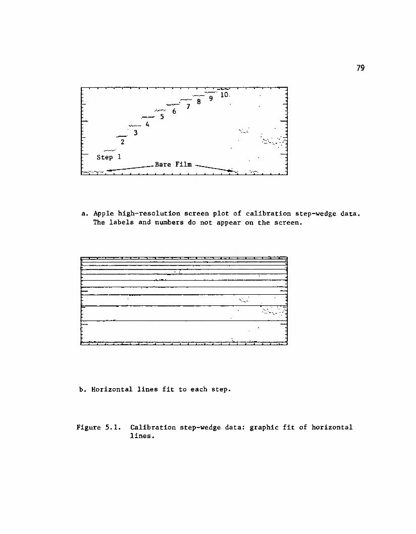
79

Step 1Bare Film

a. Apple high-resolution screen plot of calibration step-wedge data. The labels and numbers do not appear on the screen.

-

-

—

w'-

nr7

-

■

b. Horizontal lines fit to each step.

Figure 5.1. Calibration step-wedge data: graphic fit of horizontal lines.

These formulas were obtained from the Hewlett-Packard HP-25 Applications Programs booklet, Hewlett-Packard Company 1975, p. 92.

This curve-fitting operation produces a "calibration curve" from which the densitometer output voltages ("deflections") at any point on the wood specimen can be transformed into the "areal" density of the wood at that point by solving the regression equation. The estimated value y for any deflection x is given by

y = a ebx ,Oand is expressed in g/cm . The "areal" density may then be

divided by the thickness of the specimen to give wood density in g/cm^. The solution of the regression equation is performed by other programs, after the data are edited.

Program CALIBRATE prints the coefficients a and b,othe value of r , and the deflection values of the bare film

and ten wedge steps, for use by later programs. An Epson MX-80 dot matrix printer is used. See Appendix B for program listing and sample printout.

Identification of Ring Boundaries

Search for Maximum Latewood Densities— Program GETMAXThe next program to be used is called GETMAX. This

program attempts to identify the position-in-file of the

80

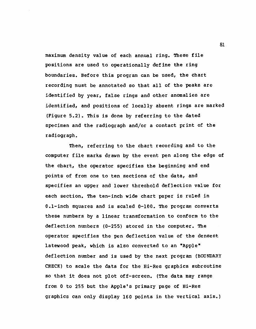
81

maximum density value of each annual ring. These file positions are used to operationally define the ring boundaries. Before this program can be used, the chart recording must be annotated so that all of the peaks are identified by year, false rings and other anomalies are identified, and positions of locally absent rings are marked (Figure 5.2). This is done by referring to the dated specimen and the radiograph and/or a contact print of the radiograph.

Then, referring to the chart recording and to the computer file marks drawn by the event pen along the edge of the chart, the operator specifies the beginning and end points of from one to ten sections of the data, and specifies an upper and lower threshold deflection value for each section. The ten-inch wide chart paper is ruled in 0.1-inch squares and is scaled 0-100. The program converts these numbers by a linear transformation to conform to the deflection numbers (0-255) stored in the computer. The operator specifies the pen deflection value of the densest latewood peak, which is also converted to an "Apple" deflection number and is used by the next program (BOUNDARY CHECK) to scale the data for the Hi-Res graphics subroutine so that it does not plot off-screen. (The data may range from 0 to 255 but the Apple's primary page of Hi-Res graphics can only display 160 points in the vertical axis.)

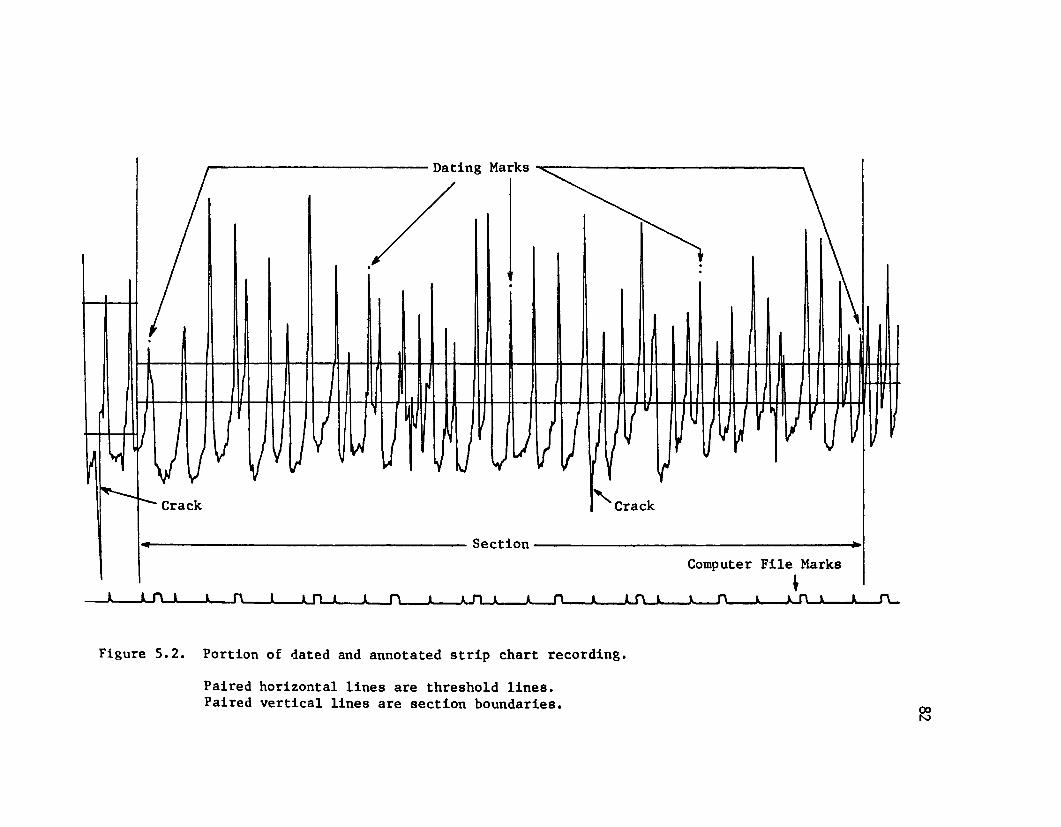
Dating Marks

Crack Crack

SectionComputer File Marks

JLTLJL

Figure 5.2. Portion of dated and annotated strip chart recording.

Paired horizontal lines are threshold lines. Paired vertical lines are section boundaries

83The two deflection thresholds specified by the

operator define a "buffer zone" to stabilize the program so that it does not regard the hundreds of minor fluctuations in the density profile as ring boundaries. The program scans the data, and after crossing an upper threshold it then waits for the data to cross the lower threshold and identifies and remembers the two crossing points (Figure 5.3). Thus multiple successive crossings of the same threshold level are ignored. This "buffer zone" technique is analogous to the use of a hysteresis loop to stabilize an electronic voltage-level detector circuit, such as a Schmidt trigger or a zero-crossing detector (Coughlin and Driscoll 1977, Ch. 4). When the program has identified all the successive upper/lower crossing pairs, the data are then searched between pairs to locate the maximum values. Numbers corresponding to the positions-in-file for each maximum are then stored on disk as sequential text files.

Figure 5.4 shows chart recordings of two specimens. One is of Sitka spruce ( Pioea sitohensis ) with very wide rings and similar values in all years for latewood maxima and earlywood minima, respectively. The other is of Jeffrey pine ( Pinus jeffreyi ) with relatively narrow rings and much more variation in earlywood and latewood densities. The Sitka spruce specimen can be easily handled in a single section, but it is much more convenient to separate the

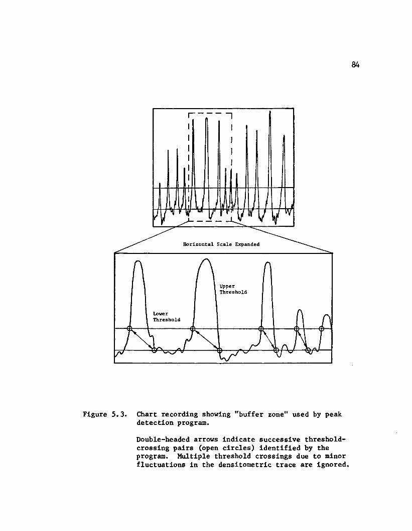
84

Horizontal Scale Expanded

---- 1

LowerThreshold

UpperThreshold

Figure 5.3. Chart recording showing "buffer zone" used by peak detection program.

Double-headed arrows indicate successive threshold- crossing pairs (open circles) identified by the program. Multiple threshold crossings due to minor fluctuations in the densitometric trace are ignored.

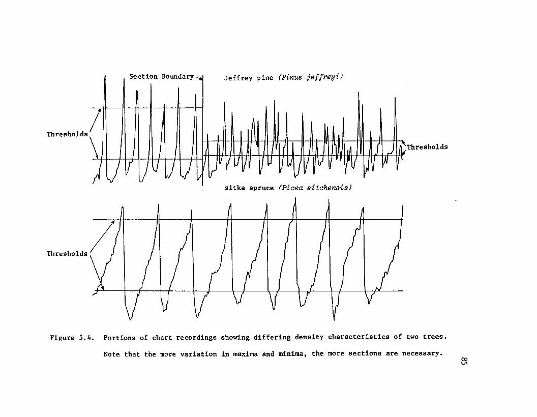
Thresholds

Jeffrey pine (Pinus jeffreyi)Section Boundary

sitka spruce (Picea eitahensis)

Thresholds

Thresholds

Figure 5.4. Portions of chart recordings showing differing density characteristics of two trees.

Note that the more variation in maxima and minima, the more sections are necessary.

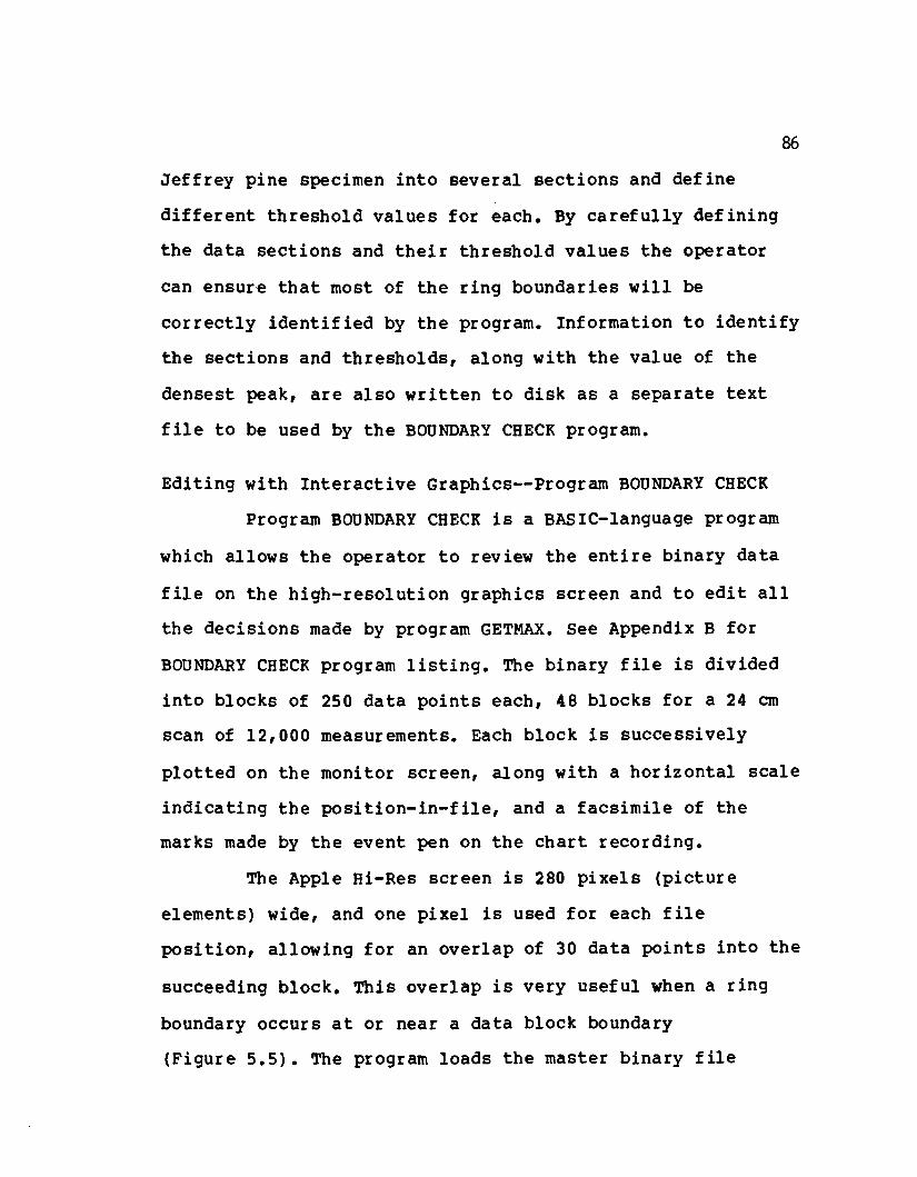
86Jeffrey pine specimen into several sections and define different threshold values for each. By carefully defining the data sections and their threshold values the operator can ensure that most of the ring boundaries will be correctly identified by the program. Information to identify the sections and thresholds, along with the value of the densest peak, are also written to disk as a separate text file to be used by the BOUNDARY CHECK program.

Editing with Interactive Graphics— Program BOUNDARY CHECKProgram BOUNDARY CHECK is a BASIC-language program

which allows the operator to review the entire binary data file on the high-resolution graphics screen and to edit all the decisions made by program GETMAX. See Appendix B for BOUNDARY CHECK program listing. The binary file is divided into blocks of 250 data points each, 48 blocks for a 24 cm scan of 12,000 measurements. Each block is successively plotted on the monitor screen, along with a horizontal scale indicating the position-in-file, and a facsimile of the marks made by the event pen on the chart recording.

The Apple Hi-Res screen is 280 pixels (picture elements) wide, and one pixel is used for each file position, allowing for an overlap of 30 data points into the succeeding block. This overlap is very useful when a ring boundary occurs at or near a data block boundary (Figure 5.5). The program loads the master binary file

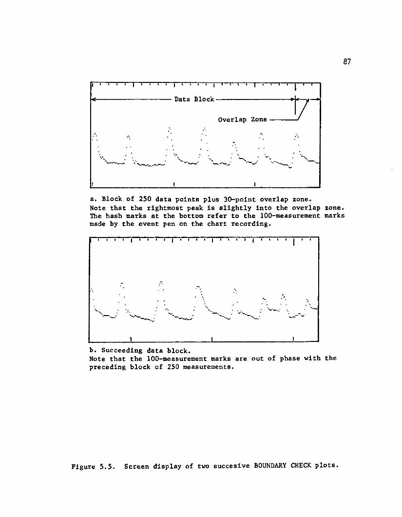
87

Data Block

Overlap Zone

a. Block of 250 data points plus 30-point overlap zone.Note that the rightmost peak is slightly into the overlap zone. The hash marks at the bottom refer to the 100-measurement marks made by the event pen on the chart recording.

b. Succeeding data block.Note that the 100-measurement marks are out of phase with the preceding block of 250 measurements.

Figure 5.5. Screen display of two succesive BOUNDARY CHECK plots.

88(collected from the densitometer scan by the TRIGGER program), the sequential text file produced by GETMAX containing the latewood maximum density positions, and the other GETMAX text file concerning the search sections and thresholds and the height of the densest peak.

BOUNDARY CHECK uses a short assembly-language program called PLOT which functions as a high-speed subroutine to do the actual plotting of each block of data. See Appendix B for the assembly-language and machine-code listings. Previous versions of BOUNDARY CHECK used a BASIC-language plotting subroutine which took several seconds to execute for each block, and made the editing task rather tedious and time-consuming. The assembly-language PLOT subroutine reads the value of the highest peak from the GETMAX file, offsets the data so that they do not plot off-screen and plots the block of 280 data points in much less than one second.

The BOUNDARY CHECK program overlays the corresponding GETMAX threshold levels on the data plot and then draws a pointer to the top of the first peak in the GETMAX peak position file (Figure 5.6). The operator may accept or reject each measurement by a single keystroke. If the "L" key is depressed, the measurement is accepted and a line drawn from below the peak to indicate this. The year, deflection value, and file position are printed on the Apple

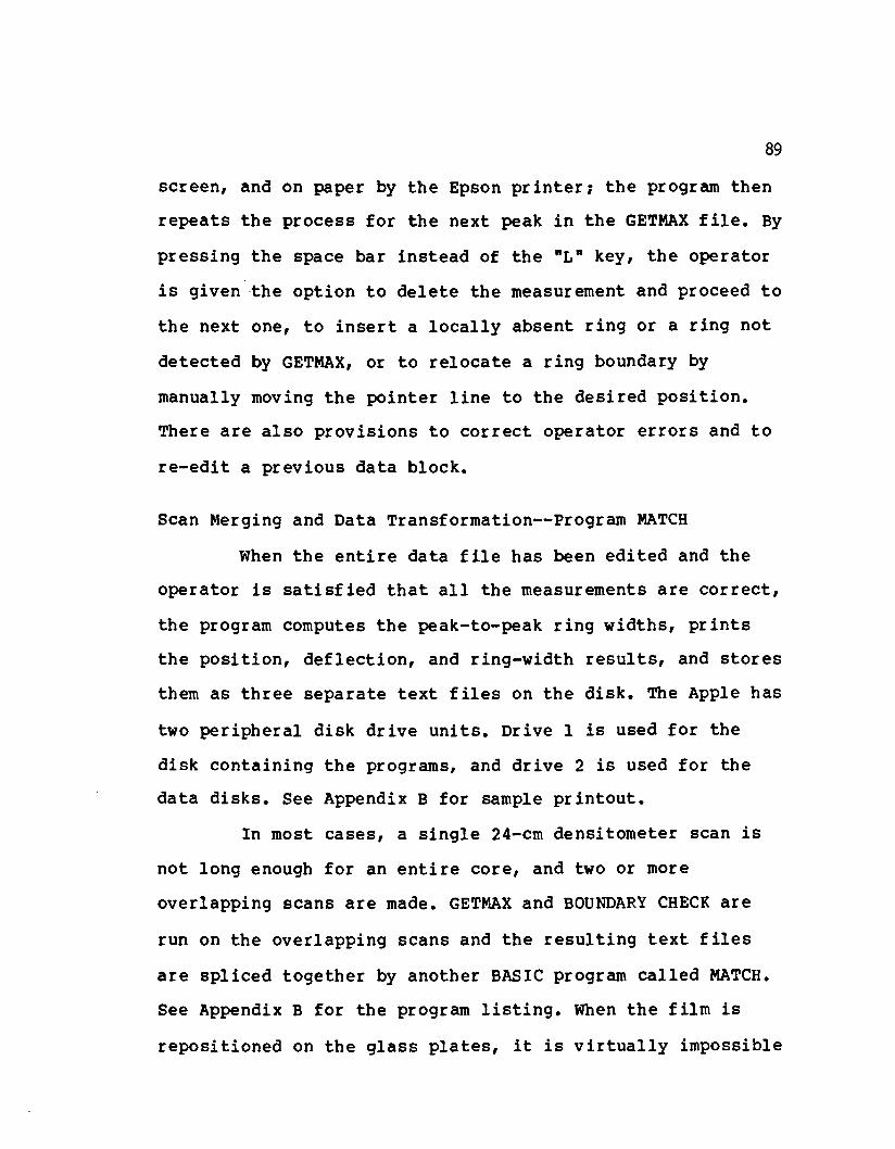
89

screen, and on paper by the Epson printer? the program then repeats the process for the next peak in the GETMAX file. By pressing the space bar instead of the "L" key, the operator is given the option to delete the measurement and proceed to the next one, to insert a locally absent ring or a ring not detected by GETMAX, or to relocate a ring boundary by manually moving the pointer line to the desired position. There are also provisions to correct operator errors and to re-edit a previous data block.

Scan Merging and Data Transformation— Program MATCHWhen the entire data file has been edited and the

operator is satisfied that all the measurements are correct, the program computes the peak-to-peak ring widths, prints the position, deflection, and ring-width results, and stores them as three separate text files on the disk. The Apple has two peripheral disk drive units. Drive 1 is used for the disk containing the programs, and drive 2 is used for the data disks. See Appendix B for sample printout.

In most cases, a single 24-cm densitometer scan is not long enough for an entire core, and two or more overlapping scans are made. GETMAX and BOUNDARY CHECK are run on the overlapping scans and the resulting text files are spliced together by another BASIC program called MATCH. See Appendix B for the program listing. When the film is repositioned on the glass plates, it is virtually impossible

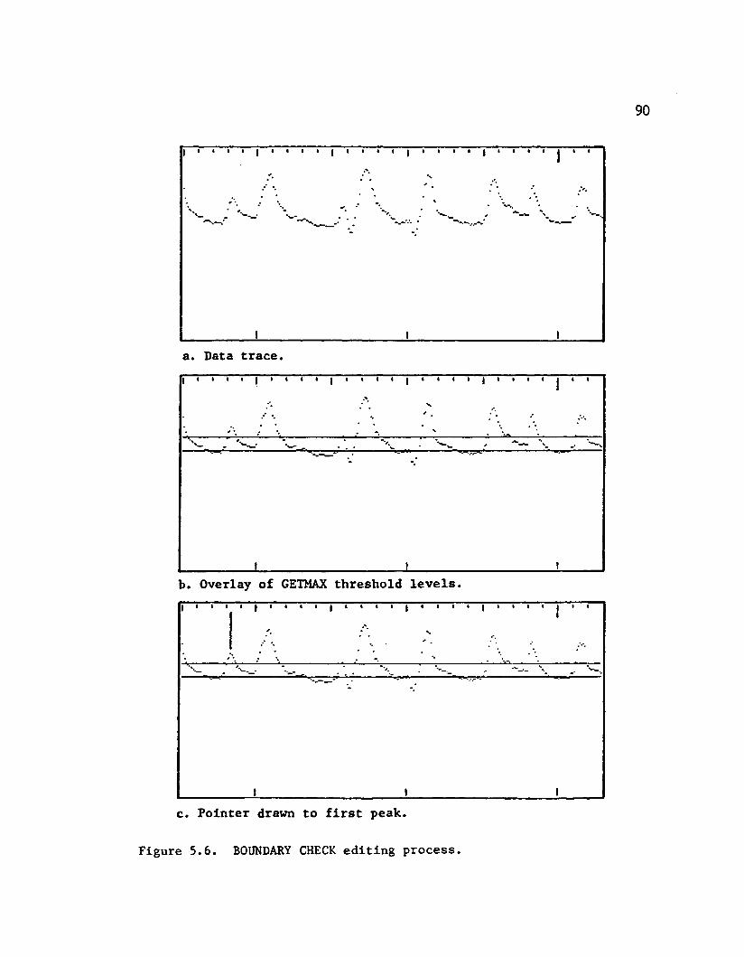
Data trace

b. Overlay of GETMAX threshold levels.

c. Pointer drawn to first peak

Figure 5.6. BOUNDARY CHECK editing process

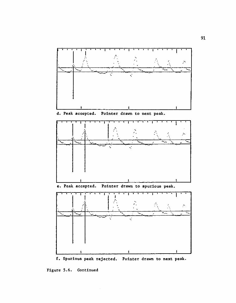
91

Figure 5.6. Continued

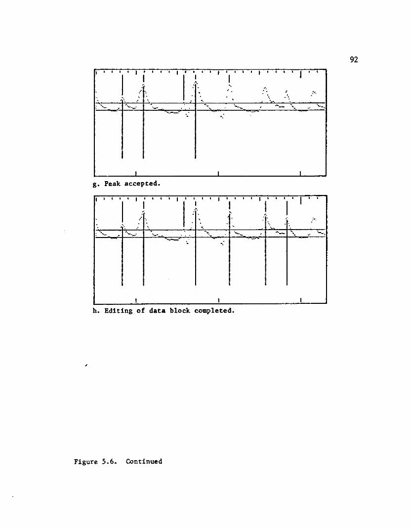
acceptedPeak

h. Editing of data block completed.

Figure 5.6. Continued

93

to realign the film and plates accurately enough so that the scan is continued precisely down the same line. Because of this problem, and the probability that some optical or electronic "drift" may occur when the optical plates and film are repositioned, there are usually some minor discrepancies in the two sets of overlapping density measurements. Program MATCH computes the average difference in peak deflections for the overlapping portion, adjusts the values in the file towards the center of the tree up or down by this amount, and then appends that file to the file which includes the outermost or bark portion of the sample. The ring width files are also combined, and the program provides a printed listing of the deflections and ring width values in standard format.

Program MATCH also performs the transformation of deflection values to wood density estimates for the entire file by solving the regression equation from page 80. MATCH uses as input the coefficients a and b from program CALIBRATE, the core thickness measured during specimen preparation, and the text file containing the deflection numbers. A standard-format listing of the maximum latewood density estimates is printed and all of the composite files produced by MATCH are stored as text files on the disk. See Appendix B for sample printout.

94

Other Programs— GETMIN, BC-MIN, AVDENProgram GETMIN identifies earlywood minimum density

positions. This BASIC program loads the master binary file and the edited and corrected GETMAX latewood maximum position file, which by now represents the correct positions of all the ring boundaries. GETMIN simply searches between the ring boundaries for the minimum values and stores the results on disk as another text file. The operator then reviews the data with program BC-MIN, which is nearly identical to BOUNDARY CHECK, but is specifically tailored to editing earlywood minimum data. Since the edited and corrected GETMAX file is used as a search template by GETMIN, usually only a very few corrections need be made by the operator, except where there are cracks in the wood specimen. Cracks occur as very low-density "blips" on the density profile (Figure 5.2), and where they occur, they are invariably chosen by GETMIN as the earlywood minimum. The operator merely remeasures the lowest-density portion of the earlywood in these rings. See Appendix B for GETMIN and BC-MIN listings.

BC-MIN does not compute minimum-to-minimum ring-width values, but simply edits the GETMIN file and creates a corresponding deflection file. Program MATCH may then be used to combine overlapping files and to compute an earlywood minimum density file.

95

Program AVDEN, also a BASIC-language program, computes average densities for each ring. Since the deflection values are logarithmically related to density, they must be converted to densities before they can be averaged. AVDEN loads the master binary file and the edited GETMAX file for ring boundary positions. Then, after input of the a and b coefficients and the specimen thickness, the program converts each of the 12,000 deflection measurements to wood density and calculates averages between successive ring boundaries. The average densities for each ring are stored on the disk as a text file, but the individual data point conversions are not saved. The program also has a provision for estimating bulk density of the entire core or any portions of the core by averaging all the density estimates between any two specified points.

The bulk-density determination allows the accuracy of the X-ray densitometry technique to be checked by comparison with bulk density measured by the gravimetric method. A bulk sample of Sitka spruce was provided by Mr. J. A. Evertson, editor of the Wood Microdensitometry Bulletin, to participate in the "Interlaboratory Standardization Survey" (Evertson 1982). The gravimetricbulk density determined on the specimen at this laboratory

3 3was 0.40 g/cm , compared to a bulk density of 0.39 g/cmcomputed by the AVDEN program using x-radiographic data.

96AVDEN also computes "integrated ring density" for

each ring, which is the integral of the annual ring density profile with respect to its width. This is done by simply multiplying the average density of the ring, in g/cm 3, by the ring width (in centimeters) to give g/cm^. This integral expresses the annual wood production of the tree (at the height of the core sample) in grams of wood tissue per square centimeter of cambial area.

CHAPTER 6

SUMMARY AND DISCUSSION

Sample Collection and Preparation Field collection presents no special problems unique

to X-ray densitometry, except that care should be taken to ensure that the cores are taken at reasonably close to right angles to the vertical boundaries of the rings. Mounting and surfacing cores to a precise thickness for radiography is a much more exacting process than surfacing cores for optical ring-width analysis. The use of special basswood or poplar densitometry mounts with the custom-made router-planer device allows the cores to be machined to their approximate final dimensions. The hand-held orbital "Speedblock" sander does an excellent job of finishing the cores to the final dimensions and producing an optically datable surface. Cores are routinely cut to a final thickness of about one millimeter with a coefficient of variation of less than five percent using this technique. For cores with very narrow rings (0.3 mm or so), at varying angles to the axis of the core, 1.0 mm is too thick to allow good resolution of all the ring boundaries without employing multiple-angle radiography. Further experimentation on the preparation of thinner core specimens (0.5 mm) is underway.

97

98Data from cores containing minor amounts of resin

may sometimes be used, but the presence of dense resin pockets can be very troublesome, especially where minimum earlywood densities, average densities, or annual integrals are to be estimated. No routine procedure has been developed at this laboratory to remove quickly and easily all the resinous material from X-ray densitometric samples. The current emphasis is on radiography of generally resin-free cores, but it is planned to devote some attention to the solution of this problem in the near future.

RadiographyThe scanning method of radiography produces high

quality contact radiographs relatively quickly and conveniently. The present equipment configuration reduces the parallax error to that equivalent to an 18 meter standoff distance in the static technique. Regulation of the line current helps to ensure a sufficiently stable X-ray source. A high quality adjustable-speed translation device allows the film to be scanned at a precisely controlled speed, producing a uniform X-ray dosage over the entire specimen. Dosage variations arising from the 60 Hz pulsing of the self-rectified X-ray tube and from the minor regular oscillation in scan speed related to the pitch of the lead-screw can be damped to below the threshold of detection by the choice of a large distance-to-velocity ratio.

99Adequate noise damping can be easily achieved at a scan speed of about 5 mm/sec. and a target-source distance of 37 cm. At this distance the loss of X-ray beam power due to lateral spread and air absorption is relatively small, allowing most specimens to be radiographed within a three-minute exposure.

A cellulose-acetate calibration standard is radiographed with each wood specimen. This standard provides data used to convert optical film densities to wood specific gravity estimates. Because each specimen is calibrated individually, it is acceptable to vary the radiation dosage from run to run, and differences in degree of film development due to minor variations in developing time, solution temperature, and the age and strength of the developer solution are unimportant, with individual calibration it is not necessary to measure the absolute optical density of the film. Only the relative optical densities of the specimen and calibration standard wedge steps need be measured by the optical densitometer.

The X-ray source may be tilted to vary the angle of incidence of the X-ray beam. In this way specimens with ring boundaries slanted with respect to the vertical axis may be radiographed with the radiation passing parallel to the ring boundaries. In many dendrochronologically sensitive trees the ring boundaries are not parallel within a single core,

100requiring that the specimen be radiographed from two or more angles (multiple-angle radiography). The radiation path length through the wood and the target-source distance is increased when the X-ray beam is at other than right angles to the core, resulting in increased absorption and less film darkening. But, since the path length is increased by the same factor for the calibration wedge, no additional calculations need be made. All of the radiographs at the various angles for a single core are then scanned separately on the densitometer, each resulting computer file is run through the standard programs, and a set of composite density estimates is spliced together using program MATCH.

Optical DensitometryThe major problem in the optical densitometry phase

so far has been to adapt the Joyce-Loebl Mk III CS microdensitometer to the task of producing large computer files of optical density measurements along a single scan of film with each measurement precisely related to its position along the scan.

A signal-conditioning amplifier has been built to make the densitometer output signal compatible to both the external strip-chart recorder and the analog-to-digital converter used by the Apple computer. An external drive assembly is used to provide a constant slow scan speed to the densitometer specimen table. This device consists of a

101motor-driven precision lead-screw and half-nut assembly fitted with an optical shaft encoder. The output pulses of the shaft encoder provide input for a digital logic circuit which in turn provides timing pulses to the Apple computer and to the event pen of the chart recorder. This logic circuit sends a pulse to trigger the Apple to read the A/D converter output at every 0.02 mm increment of film specimen travel, and sends other pulses to mark the edge of the chart recording at every 100 and every 250 Apple readings. The chart recording is thus clearly marked with respect to the position-in-file of the numbers which are collected by the computer and saved on magnetic disk in a binary file of 12,000 8-bit numbers. Each optical density measurement in the file corresponds to a displacement change of 0.02 mm along the core.

Sample RateIt is planned in the near future to double the

measurement sampling rate from every 0.02 mm to every 0.01 mm of specimen displacement, so that density-derived ring-width measurements can be reported to the nearest 0.01 mm, as is standard practice with optically measured ring-widths. The data-recording program TRIGGER will be rewritten using an assembly-language subroutine since the current BASIC subroutine is just barely fast enough in execution to read the timing pulse and the A/D converter at

102the present rate of about 30 measurements per second. The existing 48K RAM memory configuration of the Apple is large enough to handle the increased size of the data collection file (24,000 numbers), but is too small to allow the entire file to be loaded with the data manipulation programs utilizing high-resolution graphics.

Limited Length of Scan TableThe 24 cm length of the specimen scan table makes

for a great deal of inconvenience in scanning a typical specimen, almost all of which require more than one overlapping scan. There is no means by which to precisely position the film with respect to the y-axis, and as a result it is virtually impossible to continue the scan along the exact same line on the x-axis (radial direction) of the core. Additionally, a large amount of time and effort must be spent later in splicing the edited files together. A great many different files are created on the disk for each core and the procedure is confusing and time-consuming.

The obvious solution would be to construct a longer specimen table for the Joyce-Loebl instrument which could utilize the full 45 cm traverse capability of the precision lead-screw drive unit. The present 48K RAM configuration of the Apple would not be adequate for the uninterrupted collection of 45,000 data points, since the Disk Operating System (DOS) requires the use of about 10K of the available

RAM. This problem is discussed further in the section on RAM Memory Limitations. This would be a fairly difficult and expensive solution since there is very little optical tolerance on the position of the film between the condenser and objective lenses of the densitometer. Even a slight vertical movement of the film during a scan causes loss of focus at the final aperture. Another possible solution is to use the 45 cm lead-screw device with the prototype dedicated instrument described in Chapter 4. The design of this machine does not require the film to be positioned so precisely between the condenser and projection lenses, and the construction of a long film holder is a much less critical process. The 48 cm prototype film holder is made of wood and performs very well.

Densitometer ResolutionOn many cores the horizontal ring boundary angle

(cross-sectional view) is not at right angles to the long axis of the core. Since the final collimating aperture of the densitometer is not rotatable it is not possible to align the long axis of the aperture rectangle with the ring boundaries. Therefore only a fraction of the light passing through the portion of the film corresponding to the densest part of the latewood is projected onto the photomultiplier at any one time (Figure 4.8). This causes the measured peak latewood density to be depressed from its actual value and

104causes the latewood band to appear wider than it actually is. Since the total area of the aperture must be kept constant during a scan, it is not possible to change its vertical dimensions when a poorly aligned ring is encountered. Moreover, it is not possible to see the film or its projected image clearly enough to distinguish the ring boundary angles during a run.

One solution to this problem is to reduce the vertical dimension of the slit so that the aperture is in the shape of a square for the entire scan of the film. This produces a very "noisy" record since the total amount of light reaching the photomultiplier is drastically reduced. The output signal must be greatly amplified, along with the inherent random electrical noise of the system, leading to a low signal-to-noise ratio. Also, the wood is not homogeneous at this scale (less than 0.1 mm), and sharp density variations due to individual cell walls and lumens may become apparent in radiographs of exceptional clarity.

Another solution is to make two scans of the film, one with the aperture shape a standard rectangle, and the other with the vertical dimension reduced so that the aperture is square. Then the standard computer programs can be run on both data sets and a composite set of measurements spliced together. This approach is very tedious and time-consuming.

105When the rings are very narrow they often cannot be

resolved at the the standard 0.2 mm X 2.0 mm aperture setting, especially if the problem is compounded by poor alignment of the rings (Figure 4.9). The theoretical effective resolution of 0.04 mm X 0.4 mm at this setting is almost never achieved in practice due to the difficulties involved in seeing and focusing the film image on the final aperture screen, where the ring boundaries are discontinuous across the core, due to damage or wedging out, no single scan line can ensure detection and measurement of every ring (Figure 4.10). Since neither the specimen nor its projected image can be clearly seen while scanning, it is not practical to adjust the scan path during a run.

The design of the dedicated optical densitometer described in Chapter 4 would provide an effective solution to the problem of densitometer resolution. Since a clear image of a large portion of the film may be seen, it would be a reasonably simple task for the operator to adjust the scan path and aperture angle as necessary during the scan.

Data Manipulation and Calibration

CalibrationThe optical density measurements from the

X-radiographs of the core specimens are transformed to wood specific gravity estimates by comparison with the optical

106

densities of the cellulose-acetate step-wedge standard. Program CALIBRATE fits a least-squares exponential regression curve to the gravimetrically determined "areal" densities (g/cm^) of each step of the ten-step plastic calibration wedge and to the numbers corresponding to the densitometer output voltages from the corresponding steps on the radiographs. The coefficient of determination (r̂ ) is typically 0.99 or better. Each step on the wedge represents an increase in "areal" density of 0.031 g/cm^. This curve-fitting operation produces a "calibration curve" from which the densitometer output voltage at any point on the radiograph of the core can be transformed into the "areal" density of the wood at that point by solving the regression equation. The "areal" density (g/cm^) is then divided by the thickness (in cm) of the individual wood specimen to give an estimate of the wood density in g/crn̂ . The transformations are performed by programs MATCH and AVDEN.

Program AVDEN also computes bulk sample density by averaging all the density measurements between any two specified points on the core. This quantity provides a useful check on the overall accuracy of the radiographic method of density determination, since bulk sample density may also be determined gravimetrically, and the radiographic and gravimetric bulk densities may be compared on selected specimens.

107Data Manipulation

The primary task in the data manipulation phase is to edit the very large data files (several thousand numbers per core) and to produce one number per ring for each of the growth characteristics of dendrochronological interest, such as maximum latewood density, minimum earlywood density, average density of each ring, and total ring width.

The first step is to identify the positions of the annual ring boundaries. This is initially done by program GETMAX, which attempts to locate and identify the positions of the latewood maxima. The preliminary results are then checked and edited by the operator using the high-resolution graphics routines of program BOUNDARY CHECK. This program edits and corrects the GETMAX file, produces a new file of the annual latewood maxima corresponding to the GETMAX positions, and computes the total ring widths between maxima.

Program GETMIN locates the earlywood minimum positions, using the edited GETMAX position file as a guide. These positions are then edited with the aid of BC-MIN, which is very similar to BOUNDARY CHECK. BC-MIN then creates a new file of optical densities of the earlywood minima. Program MATCH splices edited files together from overlapping densitometer scans, and converts the edited files from optical density to wood density estimates. AVDEN computes

annual wood density averages and annual wood density integrals.

Computer LimitationsRAM Memory Limitations. A major limitation in the

use of the Apple computer with the large data files produced by the densitometer scans is the size of the random-access memory (RAM). The Apple has 48K (49,152 bytes) of RAM on its main circuit board. The disk operating system (DOS) uses about 10K of this space, the high-resolution graphics "picture buffer" uses 8K, the computer reserves about 2K for other uses, and the data manipulation programs use from 4K to 8K each. Several more K of buffer space are necessary to temporarily store the edited files. The program BOUNDARY CHECK, which utilizes the Hi-Res graphics "picture buffer", requires about 30K for all these functions, leaving a maximum of 18K for data storage, which is enough for about 18,000 binary 8-bit numbers.

The data manipulation process would be greatly simplified if it were possible to combine the functions of several of these programs into one and load the programs plus all 24,000 data points from two densitometer scans into the computer at once. Obviously, it is not possible to do this with only 48K of RAM. If the sample rate is increased from 50 to 100 points per millimeter, there would be 48,000 data points for two overlapping scans (or 45,000 points for

108

a single scan of a 45 cm long specimen table), making the situation even worse.

Memory Expansion Cards. The addition of a 16K memory expansion card (or an Apple Language Card) would have the effect of relocating the disk operating system (DOS) onto the card, thus making almost the entire 48R of the main circuit board RAM available for the program and data storage, which would be just barely adequate for the collection of the 45,000 single-byte numbers using program TRIGGER. This amount of RAM would still be inadequate to load a complete data file with the subsequent Hi-Res graphics routines (BOUNDARY CHECK uses a minimum of 18K of memory space), but the data could be loaded as two separate files. Some previous versions of BOUNDARY CHECK used this sub-file approach, with workable but cumbersome results. An Apple Language Card has recently been installed in the computer, and the development of new programs to utilize the additional available memory will follow in the near future.

Another possible solution to the memory size problem is the addition of a 32K memory expansion card. This card relocates the DOS onto one 16K bank of the card, and makes the other 16K bank available as RAM memory, for a total of 64K RAM locations. Depending on the degree of "transparency", or the ease of switching to the additional

109

no16K RAM locations, this may be the more attractive solution to the memory limitation problem.

Need for Graphics Print-Out. Another problem associated with collecting measurements at 0.01 mm increments is that only the equivalent of 2.8 mm of the core may be plotted at point-for-point resolution on the Apple Bi-Res screen, which has only 280 pixels (picture elements) in the horizontal dimension. It is very desirable that the operator be able to review all of the data points, but it is often very difficult to distinguish exactly what part of the core is being seen when such a small portion of the scan is shown plotted at one time.

The markings made along the side of the strip-chart recording by the event pen are very helpful, but there is always a slight uncertainty as to the exact position of the event pen with respect to the main recording pen. There is also usually a slight discrepancy between the chart and the computer record, since the chart recorder's pen response time is slower than the analog-to-digital converter's signal conversion time. Therefore the two records look slightly different when the density signal is changing rapidly, as is the case when the rings are very narrow.

A paper printout of the successive Bi-Res screen plots would be of great advantage to the operator when editing the data. Replacement of the TYMAC printer interface

Illcard with an "intelligent" interface card such as the Grappler Card would allow the Apple to make successive Hi-Res "screen dumps" to the printer, rotated 90° with no intervening spaces. The operator would then have an exact point-for-point plot of the entire computer file, which could be referred to during the editing process. A Grappler + Printer Interface card has recently been installed in the Apple, and new programming is currently being developed to take advantage of its high-resolution graphics printout capability. Figures 5.1, 5.5, and 5.6 were prepared with the aid of Grappler "screen dumps" to the printer.

High-Resolution Graphics Limitations. The use of high-resolution graphics routines seriously limits the amount of space available to the BASIC program, especially when large data files must be loaded with the program. The primary page "picture buffer" is located in memory locations 8,192 to 16,385. Only those locations above 2048 are available for BASIC programs, leaving only 6K of program memory space when the graphics buffer is in use. This places severe restrictions on the complexity and versatility of the program.

In order to fit a minimum-requirement editing program (BOUNDARY CHECK) into this space, several inconvenient programming compromises have been made. No remark statements are used in the program, and multiple

112statements per line have been used wherever possible. These practices save a large amount of memory space, but make the program very difficult to read, edit, "debug", or change. Very few operator prompts have been included in the program. This also saves considerable space, but makes it quite difficult for new operators to learn to use the program.

The Hi-Res graphics primary page screen display is a matrix of 280 horizontal pixels by 160 vertical pixels. Four lines of text are available at the bottom of the screen below the graphics display. While a workable program has been developed with this system, a larger graphics matrix would be very desirable, so that a greater portion of the data could be viewed at one time. More text area would also be very useful to the operator in controlling the program.

Several options may be possible to help solve the graphics/text/memory problem. One option is to expand the Apple memory as much as possible by the installation of memory expansion cards and to write a large portion of the BOUNDARY CHECK program as assembly-language subroutines residing above the Hi-Res picture buffer. This solution is not very attractive because of the difficulty involved in writing, editing, debugging, and modifying assembly-language programs. Nevertheless, this approach would be the least expensive in terms of monetary expenditures.

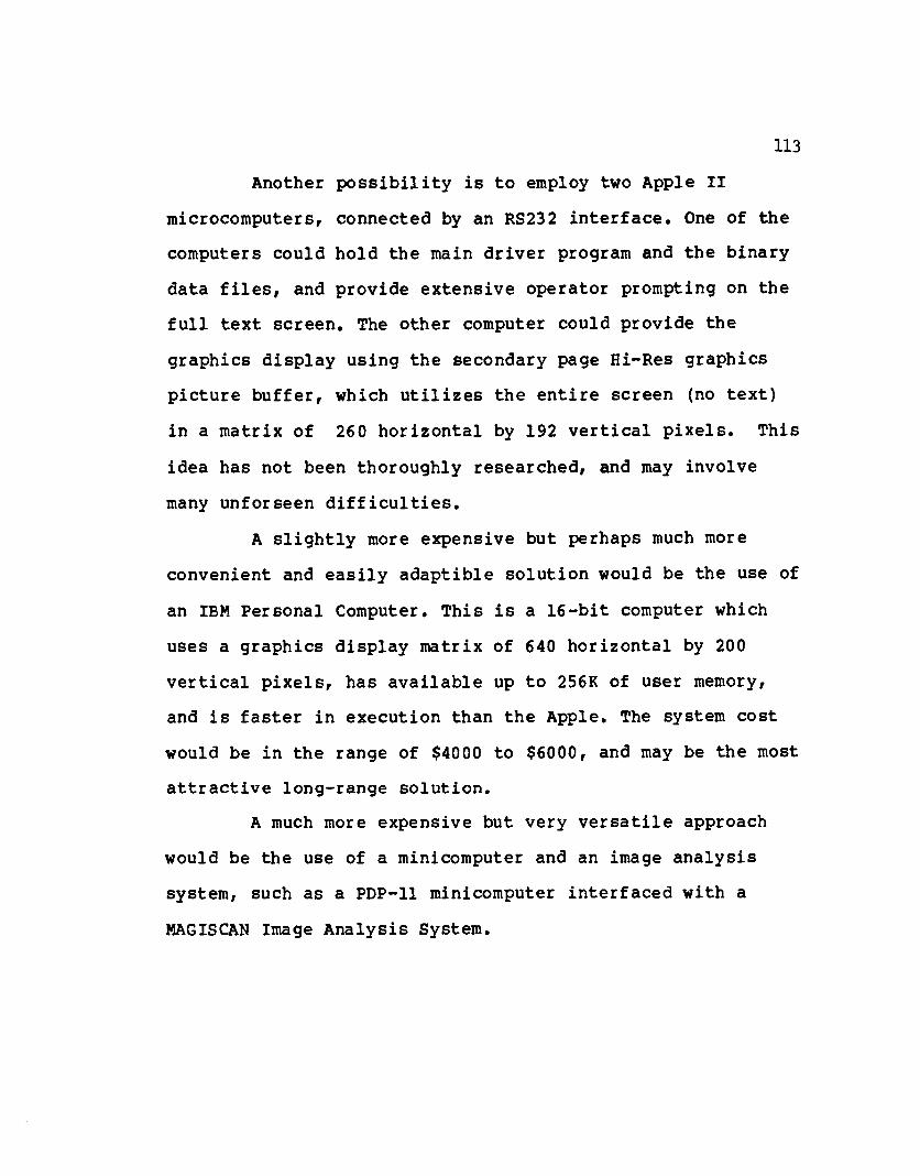
113Another possibility is to employ two Apple II

microcomputers, connected by an RS232 interface. One of the computers could hold the main driver program and the binary data files, and provide extensive operator prompting on the full text screen. The other computer could provide the graphics display using the secondary page Hi-Res graphics picture buffer, which utilizes the entire screen (no text) in a matrix of 260 horizontal by 192 vertical pixels. This idea has not been thoroughly researched, and may involve many unfor seen difficulties.

A slightly more expensive but perhaps much more convenient and easily adaptible solution would be the use of an IBM Personal Computer. This is a 16-bit computer which uses a graphics display matrix of 640 horizontal by 200 vertical pixels, has available up to 256K of user memory, and is faster in execution than the Apple. The system cost would be in the range of $4000 to $6000, and may be the most attractive long-range solution.

A much more expensive but very versatile approach would be the use of a minicomputer and an image analysis system, such as a PDP-11 minicomputer interfaced with a MAGISCAN Image Analysis System.

APPENDIX A

CIRCUIT DIAGRAMS

114

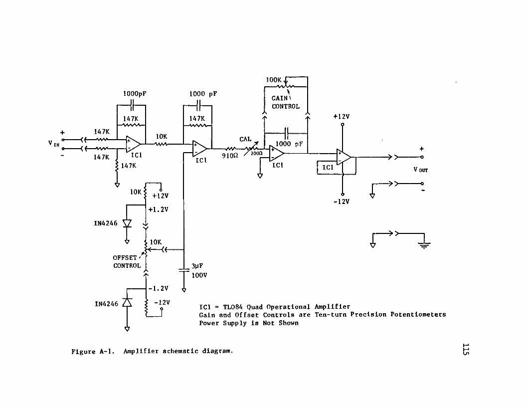
o-o

lOOOpF

147K« — v w - < (— vv\*-

147K

147K

10K

IIC1 147K

10K:

IN4246

+12V+1.2V

10K.H— (f-

OFFSETCONTROL

1000 pF

147K

3yF 100 V

100K I----A/VAyV>--

GAIN' CONTROL

/S

CAL

91 on z i0W

/tx

1000 pF

+12Vo

e >6

-12V I

f

->>

->>

■»>

+

— — o

V OUTIN4246

-1.2V V

V

ICl = TL084 Quad Operational AmplifierGain and Offset Controls are Ten-turn Precision Potentiometers Power Supply is Not Shown

Figure A-l. Amplifier schematic diagram.

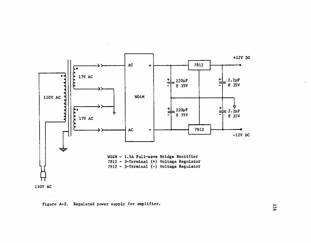
+12V DC

# *o%

110V ACecccc

«

W04M

7Q1 9

+ _ 220UF + _ 2.2yF0 35V 0 35V

+ _ 220yF 4-n= 2.2yF0 35V 0 35V

70 19-12V

W04M - 1.5A Full-wave Bridge Rectifier 7812 - 3-Terminal (+) Voltage Regulator 7912 - 3-Terminal (-) Voltage Regulator

110V AC

Figure A-2. Regulated power supply for amplifier

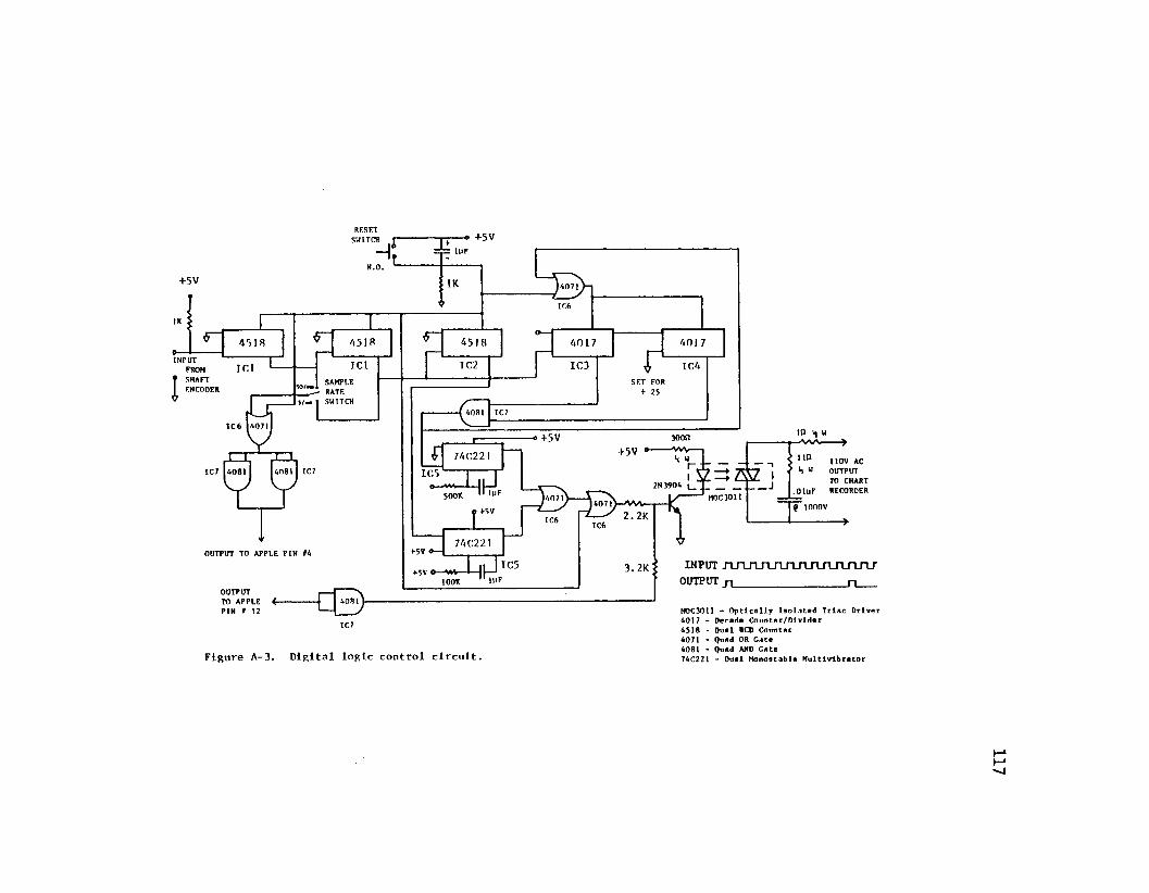
F igu re A-3. D i g i t a l l o g i c c o n t r o l c i r c u i t .

4017 - Decade Counter/Divider 4518 - Dual BCD Counter 4071 - Quad OR Gate 4081 - Quad AND Gate74C221 - Dual Monoatable Multivibrator

APPENDIX B

SOFTWARE

118

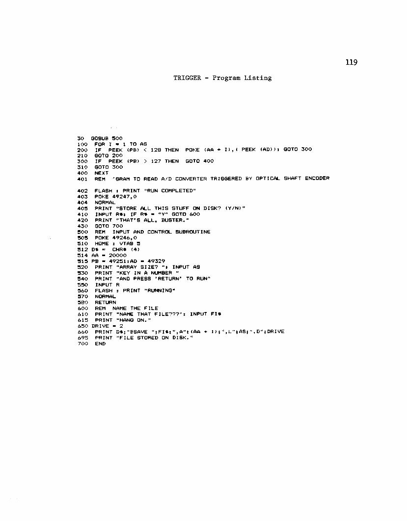
TRIGGER - Program Listing

3 0 GOSUB 5 0 01 0 0 FOR I « 1 TO AS2 0 0 IF PEEK (PB) < 1 2 8 THEN POKE <AA + I >, < PEEK <AD>>: GOTO 3 0 0 2 1 0 GOTO 2 0 03 0 0 IF PEEK (PB) > 1 2 7 THEN GOTO 4 0 0 3 1 0 GOTO 3 0 04 0 0 NEXT4 0 1 REM , GRAM TO READ A/D CONVERTER TRIGGERED BY OPTICAL SHAFT ENCODER

4 0 2 FLASH i PRINT "RUN COMPLETED"4 0 3 POKE 4 9 2 4 7 , 04 0 4 NORMAL4 0 5 PRINT "STORE ALL THIS STUFF ON DISK? ( Y / N ) "4 1 0 INPUT RSs IF RS - "Y" GOTO 6 0 04 2 0 PRINT "THAT'S ALL, BUSTER."4 3 0 GOTO 7 0 05 0 0 REM INPUT AND CONTROL SUBROUTINE5 0 5 POKE 4 9 2 4 6 , 05 1 0 HOME 3 VTAB 55 1 2 D$ = CHRS ( 4 )5 1 4 AA - 2 0 0 0 05 1 5 PB - 4 9 2 5 1 sAD - 4 9 3 2 95 2 0 PRINT "ARRAY S I Z E ? "s INPUT AS 5 3 0 PRINT "KEY IN A NUMBER "5 4 0 PRINT "AND PRESS 'RETURN' TO RUN"5 5 0 INPUT R5 6 0 FLASH 3 PRINT "RUNNING"5 7 0 NORMAL 5 8 0 RETURN6 0 0 REM NAME THE FILE6 1 0 PRINT "NAME THAT F I L E ? ? ? " 3 INPUT F I S 6 1 5 PRINT "HANG O N ."6 5 0 DRIVE ■ 26 6 0 PRINT D S ; "BSAVE " ; F I $ ; " , A"; (AA + 1 L " | A S i " , D" ; DRIVE 6 9 5 PRINT "FILE STORED ON D I S K . "7 0 0 END

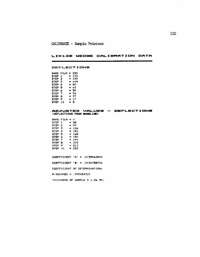
CALIBRATE - Sample Printout

L_ I K 1 2 B W E D G E CAL. I B R A T X O N D A T A

DEEL.EGT I O N SBARE FILM * 2 3 0STEP 1 * 1 7 2STEP 2 = 1 3 3STEP 3 * 1 0 4STEP 4 ■ 8 0STEP 5 * 6 2STEP 6 « 5 0STEP 7 = 3 6STEP 8 = 2 7STEP 9 = 17STEP 10 = 8

A D J U S T E D V A L U E S — D E E L E C T X O N S(DEFLECTIONS FROM BASELINE)BARE FILM - OSTEP 1 « 5 8STEP 2 = 9 7STEP 3 = 1 2 6STEP 4 = 1 5 0STEP 5 = 1 6 8STEP 6 « 1 8 0STEP 7 = 1 9 4STEP 8 = 2 0 3STEP 9 = 2 1 3STEP 10 = 2 2 2

COEFFICIENT 'A ' = . 0 1 5 5 0 6 2 8 4 4

COEFFICIENT ' B ' = . 0 1 3 6 7 5 8 7 2 6

COEFFICIENT OF DETERMINATION:

R-SQUARED = . 9 9 5 4 5 4 3 2 3

THICKNESS OF SAMPLE = 1 . 3 6 MM.

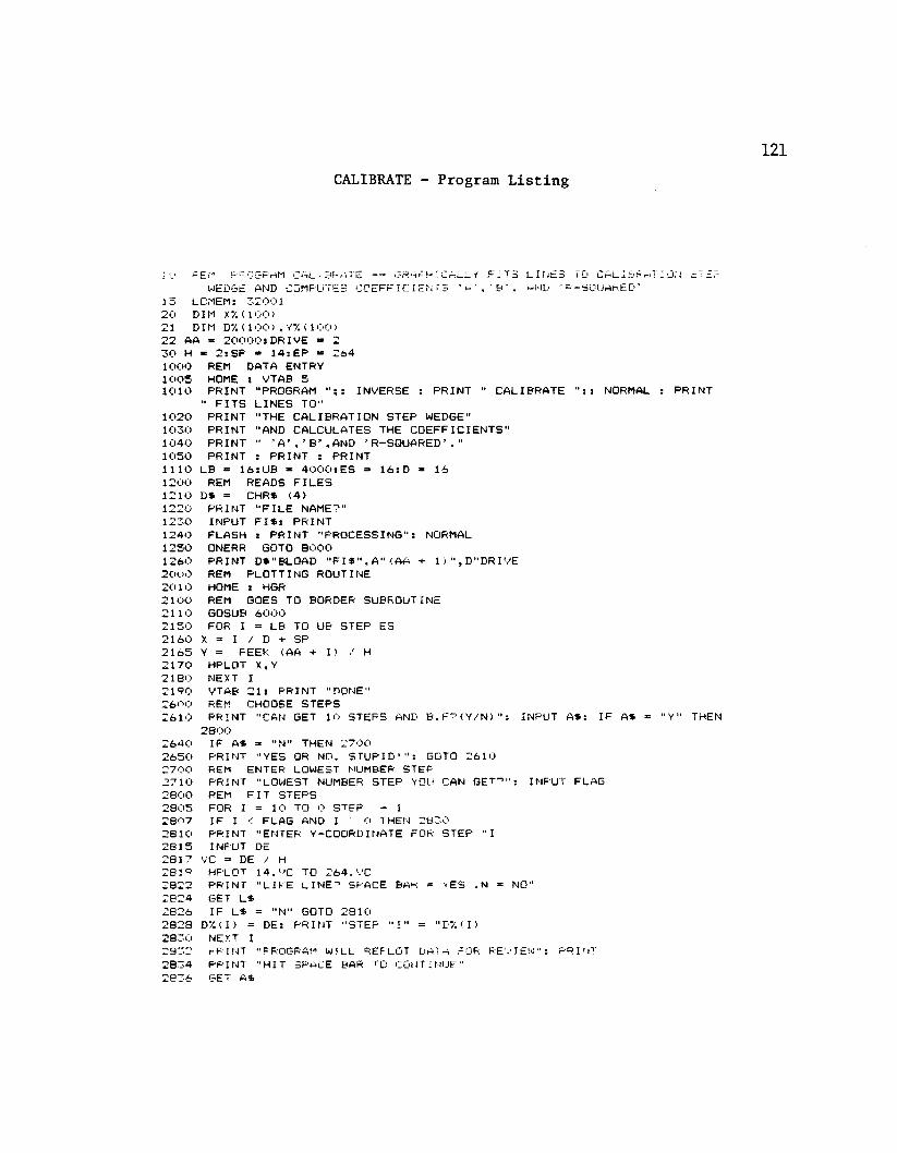
CALIBRATE - Program Listing

IV AEM PROGRAM ChL j. 3 P m TE — GRAPH I CALL/ F IT S LINES TO CALI SR>,T I UN -T£F WEDGE AND COMPUTES COEFFICIENTS NH', MB'. HMD •’ h - s q u ARED *

15 LCMEMs 3 2 0 0 12 0 DIM X-/. ( 1 0 0 )21 DIM D7. < 1 0 0 ) , Y% ( 1 0 0 )2 2 AA = 2 0 0 0 0 : DRIVE = 2 3 0 H * 2 : SR = 1 4 : EP = 2 6 4 1 0 0 0 REM DATA ENTRY 1 0 0 5 HOME : VTAB 51 0 1 0 PRINT "PROGRAM INVERSE : PRINT " CALIBRATE " ; : NORMAL : PRINT

" F IT S LINES TO"1 0 2 0 PRINT "THE CALIBRATION STEP WEDGE"1 0 3 0 PRINT "AND CALCULATES THE COEFFICIENTS"1 0 4 0 PRINT " ' A ' , 'B ' ,A N D ' R-SQUARED"."1 0 5 0 PRINT : PRINT : PRINT1 1 1 0 LB = 1 6 : UB * 4 0 0 0 : ES = 1 6 : D * 161 2 0 0 REM READS FIL E S1 2 1 0 DS = CHRS ( 4 )1 2 2 0 PRINT "FILE NAME?"1 2 3 0 INPUT F I S : PRINT1 2 4 0 FLASH : PRINT "PROCESSING": NORMAL 1 2 5 0 ONERR GOTO 8 0 0 01 2 6 0 PRINT D$"BLOAD " F IS " ,A " (A A + 1 ) " ,D"DRIVE 2 0 0 0 REM PLOTTING ROUTINE 2 0 1 0 HOME : HGR2 1 0 0 REM GOES TO BORDER SUBROUTINE2 1 1 0 GOSUB 6 0 0 02 1 5 0 FOR I = LB TO UB STEP ES2 1 6 0 X = I / D + SP2 1 6 5 Y = PEEK (AA + I ) / H2 1 7 0 HPLOT X,Y2 1 8 0 NEXT I2 1 9 0 VTAB 2 1 : PRINT "DONE"2 6 0 0 REM CHOOSE STEPS2 6 1 0 PRINT "CAN GET 10 STEPS AND B . F ? ( Y / N ) " : INPUT AS: IF AS = "Y" THEN

2 8 0 02 6 4 0 IF AS = "N" THEN 2 7 0 02 6 5 0 PRINT "YES OR NO. S T U P I D ! ": GOTO 2 6 1 0 2 7 0 0 REM ENTER LOWEST NUMBER STEF2 7 1 0 PRINT "LOWEST NUMBER STEP YOU CAN GET?": INPUT FLAG2 8 0 0 REM FIT STEPS2 8 0 5 FOR I = 10 TO O STEP - 12 8 0 7 IF I < FLAG AND I O THEN 2 8 3 02 8 1 0 PRINT "ENTER Y-COORDINATE FOR STEP "I2 8 1 5 INPUT DE2 8 1 7 VC = DE / H2 8 1 9 HPLOT 1 4 . VC TO 2 6 4 . VC2 8 2 2 PRINT "LIKE L IN E ”1 SPACE BAR = VES . N = NO"2 8 2 4 GET LS2 8 2 6 IF LS = "N" GOTO 2 8 1 02 8 2 8 DX ( I ) = DE: PRINT "STEP "I" = "D7. < I )2 8 3 0 NEXT I2 9 3 2 PRINT "PROGRAM WILL REPLOT DATA FOR REVIEW-*: PRINT2 8 3 4 PRINT "HIT SPACE BAR TQ CONTINUE"2 8 3 6 GET AS

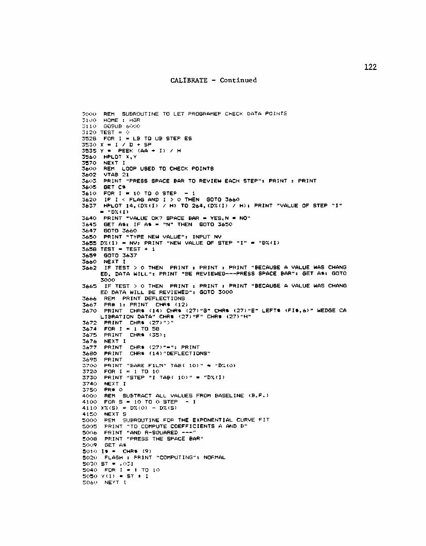
122CALIBRATE - Continued

3 0 0 0 REM SUBROUTINE TO LET PROGRAMEP CHECK DATA POINTS 3 1 0 0 HOME : HSR 3 1 1 0 GOSUB 6 0 0 0 3 1 2 0 TEST = 03 5 2 8 FOR I = LB TO UB STEP ES3 5 3 0 X = I / D + SP3 5 3 5 Y * PEEK (AA + I ) / H3 5 6 0 HPLOT X, Y3 5 7 0 NEXT I3 6 0 0 REM LOOP USED TO CHECK POINTS3 6 0 2 VTAB 213 6 0 3 PRINT "PRESS SPACE BAR TO REVIEW EACH STEP": PRINT : PRINT 3 6 0 5 GET C*3 6 1 0 FOR I - 10 TO O STEP - 13 6 2 0 IF I < FLAG AND I > 0 THEN GOTO 3 6 6 03 6 3 7 HPLOT 1 4 , (D% (I) / H) TO 2 6 4 , <D7.(I) / H) : PRINT "VALUE OF STEP "I"

« " 0 7 . (1 )3 6 4 0 PRINT "VALUE OK? SPACE BAR « YES,N * NO"3 6 4 5 GET A$: IF AS - "N" THEN GOTO 3 6 5 03 6 4 7 GOTO 3 6 6 03 6 5 0 PRINT “ TYPE NEW VALUE": INPUT NV3 6 5 5 D7. < I ) « NV: PRINT "NEW VALUE OF STEP "I" - " 0 7 . (1 )3 6 5 8 TEST « TEST + 13 6 5 9 GOTO 3 6 3 73 6 6 0 NEXT I3 6 6 2 IF TEST > O THEN PRINT i PRINT : PRINT "BECAUSE A VALUE WAS CHANG

ED, DATA WILL": PRINT "BE REVIEWED------PRESS SPACE BAR": GET AS: GOTO3 0 0 0

3 6 6 5 IF TEST > 0 THEN PRINT : PRINT : PRINT "BECAUSE A VALUE WAS CHANG ED DATA WILL BE REVIEWED": GOTO 3 0 0 0

3 6 6 6 REM PRINT DEFLECTIONS3 6 6 7 PR# 1: PRINT CHRS ( 1 2 )3 6 7 0 PRINT CHRS ( 1 4 ) CHRS ( 2 7 ) "G" CHRS ( 2 7 ) "E" LEFTS ( F I S , 6 ) " WEDGE CA

LIBRATION DATA" CHRS ( 2 7 ) "F" CHRS ( 2 7 ) "H"3 6 7 2 PRINT CHRS ( 2 7 ) " > "3 6 7 4 FOR 1 = 1 TO 5 83 6 7 5 PRINT CHRS ( 3 5 ) ;3 6 7 6 NEXT I3 6 7 7 PRINT CHRS ( 2 7 ) PRI NT3 6 8 0 PRINT CHRS ( 1 4 ) " DEFLECTIONS"3 6 9 5 PRINT3 7 0 0 PRINT "BARE FILM" TAB( 1 0 ) ' « "D%(O)3 7 2 0 FOR 1 = 1 TO 103 7 3 0 PRINT "STEP "I TAB ( 1 0 ) " = ”D 7 .( I )3 7 4 0 NEXT I 3 7 5 0 PR# O4 0 0 0 REM SUBTRACT ALL VALUES FROM BASELINE ( B . F . )4 1 0 0 FOR S = 10 TO O STEP - 1 4 1 1 0 X7. (S ) = D7. (O) - D7. (S )4 1 5 0 NEXT S5 0 0 0 REM SUBROUTINE FOR THE EXPONENTIAL CURVE FIT5 0 0 5 PRINT "TO COMPUTE COEFFICIENTS A AND B"5 0 0 6 PRINT "AND R-SQUARED ------"5 0 0 8 PRINT "PRESS THE SPACE BAR"5 0 0 9 GET AS5 0 1 0 IS = CHRS (9 )5 0 2 0 FLASH : PRINT "COMPUTING": NORMAL5 0 3 0 ST = . 0 3 15 0 4 0 FOR I = 1 TO 105 0 5 0 Y ( I ) = ST * I5 0 6 0 NEXT I

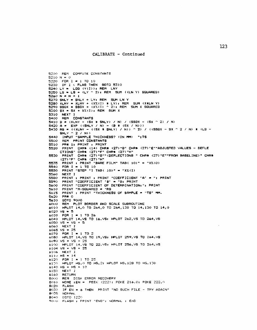
CALIBRATE - Continued

5200 REM COMPUTE CONSTANTS 5210 N = 05220 FOR I - 1 TO 105 2 5 0 IF I < FLAG THEN GOTO 5 3 1 05 2 4 0 LY « LOG < Y < I ) ) : REM LNY5 2 5 0 LS » LS + <LY ^ 2 > i REM SUM < <LN Y) SQUARED)5 2 6 0 N = N + 15 2 7 0 SNLY - SNLY 4- LY: REM SUM LN Y5 2 8 0 XLNY - XLNY + <X7. ( I ) * LY) I REM SUM (X*LN Y)5 2 9 0 SSQX - SSQX > (X7.(I> ^ 2 ) : REM SUM X SQUARED5 3 0 0 SX = SX + X7. ( I ) : REM SUM X5 3 1 0 NEXT I5 4 0 0 REM CONSTANTS5 4 1 0 B - (XLNY - (SX * SNLY) / N> / (SSQX - (SX 2 ) / N)5 4 2 0 A = EXP ( (SNLY / N) - (B * (SX / N ) ) )5 4 3 0 RS ■ ( (XLNY - ( (S X * SNLY) / N ) ) ~ 2 ) / ( (SSQX - S X " 2 / N) * (LS -

SNLY " 2 / N ) >5 4 4 0 INPUT "SAMPLE THICKNESS? ( I N MM) " ;T S 5 5 0 0 REM PRINT CONSTANTS 5 5 1 0 PR# 1: PRINT « PRINT5 5 2 0 PRINT CHRS ( 1 4 ) CHRS ( 2 7 ) "G" CHRS ( 2 7 ) "E""ADJUSTED VALUES - DEFLE

CTIONS" CHRS ( 2 7 ) "F" CHRS ( 2 7 ) "H"5 5 3 0 PRINT CHRS ( 2 7 ) "G"" (DEFLECTIONS " CHRS ( 2 7 ) "E""FROM B A S E L IN E )" CHRS

( 2 7 ) "F" CHRS ( 2 7 ) "H"5 5 3 5 PRINT i PRINT "BARE FILM" TAB( 1 0 ) " ■ "X%(0>5 5 4 0 FOR I » 1 TO 1 05 5 5 0 PRINT "STEP "I TAB( l O ) " ■ "X% (D 5 5 6 0 NEXT I5 5 8 0 PRINT : PRINT : PRINT "COEFFICIENT ' A ’ - "* PRINT 5 5 9 0 PRINT "COEFFICIENT ' B ' - "Bi PRINT 5 6 0 0 PRINT "COEFFICIENT OF D E T E R M I N A T I O N : P R I N T 5 6 1 0 PRINT "R-SQUARED - "RS5 6 1 5 PRINT : PRINT "THICKNESS OF SAMPLE - "TS" MM.5 6 2 0 PR# O 5 6 3 0 GOTO 9 0 0 06 0 0 0 REM PLOT BORDER AND SCALE SUBROUTINE6 0 1 0 HPLOT 1 4 , 0 TO 2 6 4 , 0 TO 2 6 4 , 1 3 0 TO 1 4 , 1 3 0 TO 1 4 , 06 0 2 0 VS - 56 0 3 0 FOR I * 1 TO 2 66 0 4 0 HPLOT 1 4 , VS TO 1 6 , VS: HPLOT 2 6 2 , VS TO 2 6 4 , VS6 0 5 0 VS * VS > 56 0 6 0 NEXT I6 0 6 5 VS * 2 56 0 7 0 FOR I - 1 TO 26 0 8 0 HPLOT 1 4 , VS TO 1 9 , VS: HPLOT 2 5 9 , VS TO 2 6 4 , VS 6 0 9 0 VS - VS + 2 56100 HPLOT 14,VS TO 22,VS: HPLOT 256,VS TO 264,VS6104 VS = VS + 256106 NEXT I6110 HS = 146120 FOR I = 1 TO 256130 HPLOT HS,O TO HS,2: HPLOT HS,128 TO HS,130 6140 HS * HS 4- 10 6150 NEXT I 6160 RETURN8000 REM DISK ERROR RECOVERY8010 HOME :EN = PEEK (222): POKE 216,0: POKE 222,0 8020 FLASH8030 IF EN * 6 THEN PRINT "NO SUCH FILE - TRY AGAIN"8035 NORMAL 8040 GOTO 12209000 FLASH : PRINT "END": NORMAL : END

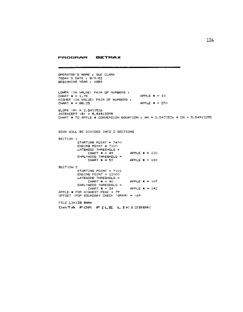
124

P R O G R A M Q E T M A X

OPERATOR'S NAME : SUE CLARK TODAY’ S DATE : 8 / 9 / 8 2 BEGINNING YEAR : 1 8 8 4

LOWER (IN VALUE) PAIR OF NUMBERS :CHART # = 1 . 7 5 APPLE # * 10HIGHER (IN VALUE) PAIR OF NUMBERS :CHART # = 8 8 . 2 5 APPLE # = 2 3 0

SLOPE (M) = 2 . 5 4 3 3 5 2 6 INTERCEPT (B) = 5 . 5 4 9 1 3 2 9 5CHART # TO APPLE # CONVERSION EQUATION s AN = 2 . 5 4 3 3 5 2 6 * CN + 5 . 5 4 9 1 3 2 9 5

SCAN WILL BE DIVIDED INTO 2 SECTIONS

SECTION 1STARTING POINT = 3 4 7 0 ENDING POINT = 7 1 0 0 LATEWOOD THRESHOLD =

CHART # = 4 9 EARLYWOOD THRESHOLD =

CHART # = 5 3

APPLE # = 1 3 0

APPLE # = 1 4 0

SECTION 2STARTING POINT = 7 1 0 1 ENDING POINT = 1 2 0 0 0 LATEWOOD THRESHOLD =

CHART # = 4 0 EARLYWOOD THRESHOLD =

CHART # = 5 4APPLE # FOR HIGHEST PEAK = 7 9 OFFSET (FOR BOUNDARY CHECK 'GRAM)

APPLE # = 1 0 7

APPLE # = 1 4 2

FILE L IK 12B BARKD A T A F ^ O F C F I L . E I_I K 1. 22 0 EE* K

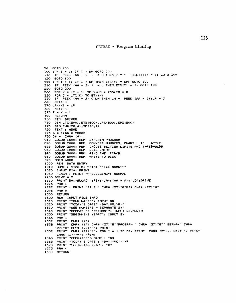
125GETMAX - Program Listing

50 GOTO 700100 1 * 1 + 1 : IF I > EP GOTO 30o110 IF PEEK (AA + I) < * H THEN Y = Y + 1 : LT7. (Y > = I: GOTO120 GOTO 1002 0 0 1 * 1 + 1 : I F I > EP THEN ETV.(Y) - EP: GOTO 3 0 0210 IF PEEK (AA + I ) > - L THEN ET%(Y) = I : GOTO 1 0 0220 GOTO 2 0 03 0 0 FOR K - (F + 1) TO Y:LM * 2 5 5 : EM - 03 2 0 FOR J - LT7.(K) TO ET%(K)3 3 0 IF PEEK (AA + J ) < LM THEN LM * PEEK (AA + J ) 8 LP * J3 6 0 NEXT J370 LP%(K) = LP3 8 0 NEXT K3 8 5 F * K - 13 9 0 RETURN700 REM DRIVER

EXPLAIN PROGRAMCONVERT NUMBERS, CHART - TO - APPLE CHOOSE SECTION LIMITS AND THRESHOLDS DATA ENTRY FIND THE PEAKS WRITE TO DISK

DIM LT%( 5 0 0 ) ,ET% ( 5 0 0 ) ,LP% ( 5 0 0 ) ,EP% ( 5 0 0 )DIM T H % ( 2 0 , 4 ) , T C ( 2 0 , 4 )TEXT i HOME

A * 1 iAA ■ 2 0 0 0 0 7 3 0 DS - CHR$ ( 4 )8 1 0 60SU B 1 5 0 0 : REM

GOSUB 2 0 0 0 8 REM GOSUB 2 5 0 0 b REM GOSUB lOOO: REM GOSUB 3 0 0 0 : REM GOSUB 5 0 0 0 8 REM GOTO 6 0 0 0

REM DATA ENTRYHOME : VTAB 5 : PRINT "FILE NAME??"INPUT F I $ : PRINTFLASH i PRINT "PROCESSING": NORMAL

1 1 0 0 DRIVE ■ 21 1 1 0 PRINT D$;"BLOAD " ; F I $ ; ", A"; (AA + A ) ; " ,D " ;D R IV E

PR# 1PRINT : PRINT "FILE " CHRS ( 2 7 ) "G "FI$ CHRS ( 2 7 ) "H PR# O RETURNREM INPUT FILE INFO PRINT "YOUR NAME?"8 INPUT NS PRINT "TODAY'S DATE? (DA Y,M O ,Y R)"PRINT "USE NUMBERS - SEPARATE BY"PRINT "COMMAS OR ' R E T U R N ' I N P U T DA,MO,YR PRINT "BEGINNING YEAR?": INPUT BY

7 1 07 1 57 2 07 2 5

8 2 08 2 58 3 08 4 08 6 08 7 01000101010201 0 6 0

1 2 7 51 2 8 21 2 9 51 3 0 01 5 0 01 5 1 01 5 2 01 5 3 01 5 4 01 5 5 01 5 5 51 5 5 71 5 5 8

1 5 5 9

1 5 6 0 1 5 6 5 1 5 7 0 1 5 7 5 1 6 0 0

PR# 1 PRINT PRINT

CHRS ( 1 2 )CHRS ( 1 4 ) CHRS ( 2 7 ) "E""PROGRAM

( 2 7 ) "H" CHRS ( 2 7 ) "F": PRINT PRINT CHRS ( 2 7 ) FOR I CHRS ( 2 7 ) " * " : PRINT PRINT "OPERATOR'S NAME : "NSPRINT "TODAY’ S DATE : "DA"/ "MO"/ " YRPRINT "BEGINNING YEAR : "BYPR# O RETURN

CHRS ( 2 7 ) "G"" GETMAX"

1 TO 5 8 : PRINT CHRS ( 3 5 ) : : NEXT

CHRS

I 8 PRI NT

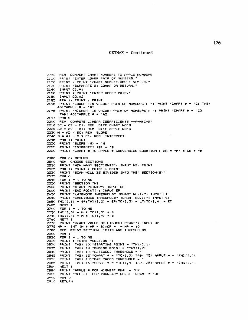
126GETMAX - Continued

2000 REM CONVERT CHART NUMBERS TO APPLE NUMBERS 2 1 1 0 PRINT "ENTER LOWER PAIR OF NUMBERS."2120 PRINT s PRINT "CHART NUMBER.APPLE NUMBER."2130 PRINT "SEPARATE BY COMMA OR RETURN."2 1 4 0 INPUT C 1 ,A 12 1 5 0 PRINT i PRINT "ENTER UPPER P A I R . "2 1 8 0 INPUT C 2 ,A 22 1 8 5 PR# 1: PRINT : PRINT2 1 9 0 PRINT "LOWER ( IN VALUE) PAIR OF NUMBERS i ": PRINT "CHART # - "Cl TAB<

4 0 ) "APPLE # - "A12 1 9 5 PRINT "HIGHER ( IN VALUE) PAIR OF NUMBERS i ": PRINT "CHART # - "C2

TAB( 4 0 ) "APPLE # » "A2 2 1 9 7 PR# O2 2 0 0 REM COMPUTE LINEAR COEFFICIENTS — A=M*C+B"2 2 1 0 DC = C2 - Cl3 REM DIFF CHART NO 'S2 2 2 0 AD * A2 - A l : REM DIFF APPLE NO 'S2 2 3 0 M « AD / DCs REM SLOPE2 2 4 0 B - A l - M * C l : REM INTERCEPT2 2 4 5 PR# I t PRINT2 2 5 0 PRINT "SLOPE <M> « "M2 2 5 5 PRINT "INTERCEPT (B) - "B2 2 6 0 PRINT "CHART # TO APPLE # CONVERSION EQUATION i AN - "M" * CN ♦ "B

2 3 0 02 5 0 02 5 2 02 5 2 52 5 3 02 5 3 52 5 4 02 5 5 02 5 8 02 6 0 02 6 2 02 6 4 02 6 8 02 6 8 52 7 0 02 7 2 02 7 4 02 7 6 02 7 7 02 7 7 52 7 8 02 8 0 02 8 2 02 8 2 52 8 3 02 8 3 52 8 4 02 8 4 52 8 5 02 8 5 528602 8 8 02 8 8 52*002 9 1 0

PR# Oi RETURNREM CHOOSE SECTIONSPRINT "HOW MANY SECTIONS?": INPUT NS: PRINTPR# 1: PRINT : PRINT % PRINTPRINT "SCAN WILL BE DIVIDED INTO "NS" S E C T IO N (S )"PR# OFOR I - 1 TO NS PRINT "SECTION "NS PRINT "START POINT?": INPUT SP PRINT "END POINT?": INPUT EPPRINT "LATEWOOD THRESHOLD? (CHART N O . ) s ": INPUT LT PRINT "EARLYWOOD THRESHOLD? (CHART N O . > s ": INPUT ET

T H % (I ,1 ) - S P : T H 7 . ( I , 2 ) - E P : T C ( I , 3 ) - L T : T C < I , 4 ) - ET NEXT IFOR I * 1 TO NS

T H % (I ,3 ) - M S T C ( I , 3 > + B TH%( 1 , 4 ) » M * T C < I ,4 > + B

NEXT IPRINT "CHART VALUE OF HIGHEST PEAK?": INPUT HP

HP * INT (M * HP + B ) : OF - - HP + 10REM PRINT SECTION LIMITS AND THRESHOLDS PR# 1FOR I * 1 TO NSPRINT : PRINT "SECTION "IPRINT TAB < 1 0 ) "STARTING POINT - "TH 7.(I , 1)PRINT TAB( 1 0 ) "ENDING POINT = " T H % (I ,2 )PRINT TAB v 1 0 ) "LATEWOOD THRESHOLD * "PRINT TAB < 15>"CHART # * " T C ( I ,3 > TAB( 3 5 ) "APPLE # PRINT TAB( 1 0 ) "EARLYWOOD THRESHOLD * "PRINT TAB( 1 5 ) "CHART # * " T C ( I ,4 > TAB( 3 5 ) "APPLE # NEXT IPRINT "APPLE # FOR HIGHEST PEAK = "HPPRINT "OFFSET (FOR BOUNDARY CHECK 'GRAM) * "OFPR# ORETURN

TH7. (1,3)TH7. (1,4;

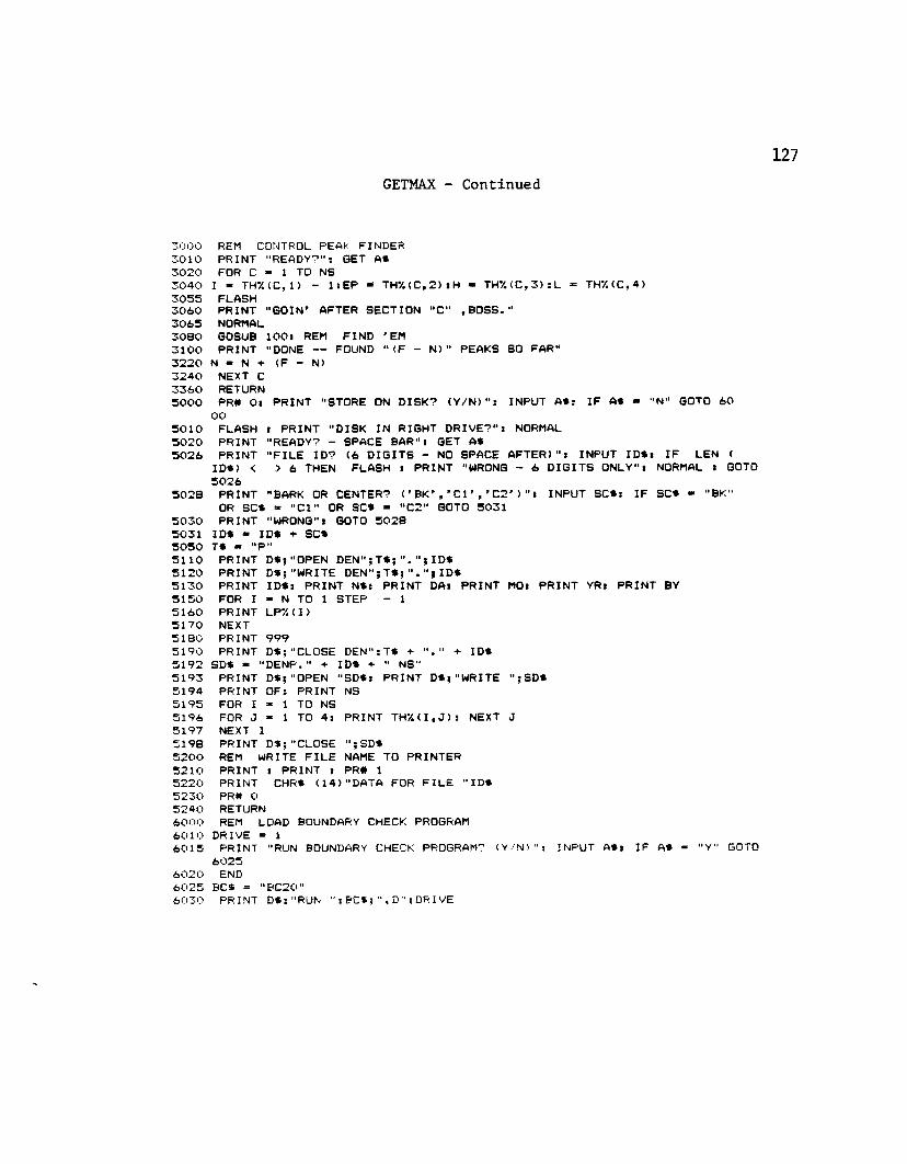
127GETMAX - Continued

3 0 0 0 REM CONTROL PEAK FINDER 3 0 1 0 PRINT "READY?"s GET A$3 0 2 0 FOR C * 1 TO NS3 0 4 0 I « TH% (C,1) - I s E P - TH% (C,2) :H « T H 7.(C ,3 ) sL = TH% (C,4)3 0 5 5 FLASH3 0 6 0 PRINT "GOIN' AFTER SECTION "C" , B O S S . "3 0 6 5 NORMAL3 0 8 0 GOSUB 1 0 0 : REM FIND 'EM3 1 0 0 PRINT "DONE — FOUND " <F - N ) " PEAKS SO FAR"3 2 2 0 N = N + (F - N)3 2 4 0 NEXT C 3 3 6 0 RETURN5 0 0 0 PR# O: PRINT "STORE ON DISK ? ( Y / N ) ": INPUT AS: IF AS - "N" GOTO 6 0

0 05 0 1 0 FLASH * PRINT "DISK IN RIGHT DR IVE ?": NORMAL 5 0 2 0 PRINT "READY? - SPACE BAR": GET AS5 0 2 6 PRINT "FILE ID ? ( 6 D IG IT S - NO SPACE AFTER)": INPUT ID S: IF LEN <

IDS) < > 6 THEN FLASH : PRINT "WRONG - 6 D IG IT S ONLY": NORMAL : GOTO 5 0 2 6

5 0 2 8 PRINT "BARK OR CENTER? < ' BK’ , ' C l ’ , ’ C 2 ' >": INPUT SOS: IF SCS - "BK"OR SCS * "C l" OR SCS • "C2" GOTO 5 0 3 1

5 0 3 0 PRINT "WRONG": GOTO 5 0 2 85 0 3 1 IDS - IDS + SCS 5 0 5 0 TS - "P"5 1 1 0 PRINT DS;"OPEN DEN"5 T S ; " . " j I D S 5 1 2 0 PRINT DS;"WRITE D E N " ; T $ ; I D S5 1 3 0 PRINT IDS: PRINT NS: PRINT DA: PRINT MO: PRINT YR: PRINT BY 5 1 5 0 FOR I * N TO 1 STEP - 1 5 1 6 0 PRINT LPV. < I >5 1 7 0 NEXT 5 1 8 0 PRINT 9 9 95 1 9 0 PRINT DS;"CLOSE DEN"; TS + " + IDS5 1 9 2 SDS * "D E N P ." + IDS + " NS"5 1 9 3 PRINT DS;"OPEN "SDS: PRINT DS;"WRITE " ; SDS5 1 9 4 PRINT OF: PRINT NS5 1 9 5 FOR I * 1 TO NS5 1 9 6 FOR J * 1 TO 4 : PRINT TH%( I , J ) : NEXT J5 1 9 7 NEXT I5 1 9 8 PRINT DS;"CLOSE " ; SDS5 2 0 0 REM WRITE F ILE NAME TO PRINTER 5 2 1 0 PRINT : PRINT : PR# 15 2 2 0 PRINT CHRS ( 1 4 ) "DATA FOR FILE "IDS 5 2 3 0 PR# O 5 2 4 0 RETURN6 0 0 0 REM LOAD BOUNDARY CHECK PROGRAM 6 0 1 0 DRIVE = 16 0 1 5 PRINT "RUN BOUNDARY CHECK PROGRAM? ( Y / N ) ": INPUT AS: IF AS = "Y" GOTO

6 0 2 5 6 0 2 0 END 6 0 2 5 BCS = "B C 2 0 "6 0 3 0 PRINT DS;"RUN " ; P C S ; " , D "; DPIVE

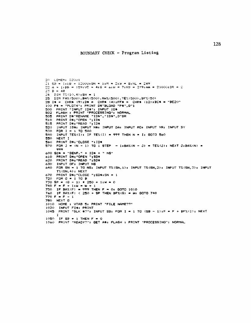
128BOUNDARY CHECK - Program Listing

2 0 LOMEM: 3 2 0 0 121 S B = 1 : U B = 1 2 0 0 0 sG N = 1 : M = 2 : B = 9 : NL = 2 4 92 2 A = 1:BB = 159:VC = 4 : S = 6:W = 7sR B = 2 7 9 : AA * 2 0 0 0 0 : DR = 22 3 B = 4 82 4 DIM T7. ( 1 0 , 4 ) :SN = 12 5 DIM FA7. (50 0 > , BA% <5 0 0 ) , RW% (50 0 > , TEX (500> , BFX (50>2 8 1$ * CHR$ ( 9 ) : D $ - CHRS ( 4 ) :F F S * CHRS ( 1 2 ) : BCS * "BC20"1 0 0 PS « "PL0T4": PRINT DS"BLOAD " P $ " ,D " 1 5 0 0 PRINT "INPUT ID S": INPUT IDS5 0 2 FLASH : PRINT "PROCESSING": NORMAL 5 0 5 PRINT DS"RENAME " I D S " , "IDS% D"DR 5 1 0 PRINT DS;"OPEN " ; IDS 5 1 5 PRINT DS;"READ " ; IDS5 2 0 INPUT IDS: INPUT NS: INPUT DA: INPUT MO: INPUT VR: INPUT BY5 3 0 FOR I = 1 TO 5 0 05 4 0 INPUT TE7. < I > : IF TEX ( I > * 9 9 9 THEN N « I : GOTO 5 6 05 5 0 NEXT I5 6 0 PRINT DS;"CLOSE " ; IDS5 7 0 FOR J * (N - 1) TO 1 STEP - 1:B AX (N - J ) » T E X ( J ) : NEXT J:BA%<N) «

9 9 96 0 0 SDS = "D E N P ." + I D S + " NS"6 1 0 PRINT DS;"OPEN " ; SDS 6 2 0 PRINT DS;"READ " ; SDS 6 3 0 INPUT OF: INPUT NS6 4 0 FOR SN » 1 TO NS: INPUT T % ( S N ,1 ) : INPUT T 7 . ( S N ,2 ) : INPUT T 7 . ( S N , 3 ) : INPUT

TX <S N ,4 ) : NEXT6 7 0 PRINT DS;"CLOSE " ;S D S :S N ■ 1 7 2 0 FOR Q * 1 TO B 7 3 0 SP » (Q - 1) * 2 5 0 ♦ 1:W » O 7 4 0 F » F + 1:W * W + 17 5 0 IF BA7.(F) ■ 9 9 9 THEN F ■ O: GOTO 1 0 1 07 6 0 IF BAX(F) < 2 5 0 + SP THEN BFX(Q) - W: GOTO 7 4 07 7 0 F - F - 17 8 0 NEXT Q1 0 1 0 HOME : VTAB 5% PRINT "FILE NAME??"1 0 2 0 INPUT F I S : PRINT1 0 4 5 PRINT "BLK # ? " : INPUT SB: FOR I ■ 1 TO (SB - 1 ) : F - F + BFX( I ) : NEXT

I1 0 5 0 IF SB * 1 THEN F « O1 0 6 0 PRINT "READY?": GET AS: FLASH : PRINT "PROCESSING": NORMAL

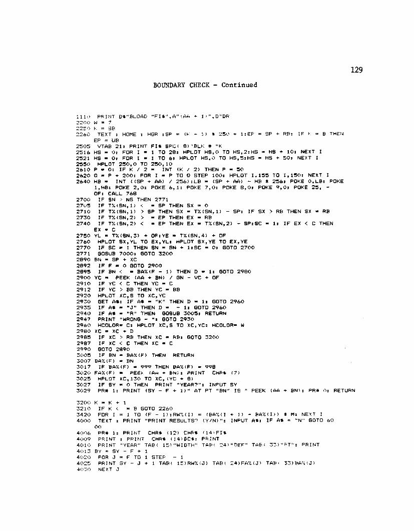
129BOUNDARY CHECK - Continued

1110 PRINT D$"BLOAD "FI$", A" '.AA > 1 ) ",D"DR 2200 W = 7 2250 K = SB2 2 6 0 TEXT s HOME : HGR : SP = (K - 1) * 2 5 0 + 1 sEP ■ SP + RBs IF K = B THEN

EP = UB2 5 0 5 VTAB 2 1 s PRINT F I S S P C ( 8 ) "BLK # "K2 5 1 6 HS = Os FOR 1 * 1 TO 2 8 s HPLOT H S , 0 TO H S ,2 s H S * HS + 10s NEXT I 2 5 2 1 HS - Os FOR I * 1 TO 6 s HPLOT H S , 0 TO H S ,5 s H S * HS + 5 0 s NEXT I 2 5 5 0 HPLOT 2 5 0 , 0 TO 2 5 0 , 1 02 6 1 0 P - Os IF K / 2 * INT (K / 2 ) THEN P * 5 02 6 2 0 Q * P + 2 0 0 s FOR I * P TO Q STEP 1 0 0 s HPLOT 1 , 1 5 5 TO I , 1 5 0 s NEXT I2 6 4 0 HB ■ INT < <SP + AA) / 2 5 6 ) sLB ■ (SP + AA) - HB * 2 5 6 s POKE 0 ,L B s POKE

1 , HBs POKE 2 , 0 s POKE 6 , Is POKE 7 , 0 : POKE 8 , 0 s POKE 9 , 0 s POKE 2 5 , - OF: CALL 7 6 8

2 7 0 0 IF SN > NS THEN 2 7 7 12 7 0 5 IF T%<SN,1) < - SP THEN SX » O2 7 1 0 IF T % (S N ,1 ) > SP THEN SX * T % (SN ,1) - SPs IF SX > RB THEN SX - RB 2 7 3 0 IF T% (SN,2> > - E P THEN EX ■ RB2 7 4 0 IF T % (SN ,2 ) < * EP THEN EX * T 7 .<SN ,2) - S P sS C - 1: IF EX < C THEN

EX - C2 7 5 0 YL « T % (SN ,3 ) -*• OF: YE « T % (S N ,4 ) 4- OF 2 7 6 0 HPLOT SX ,Y L TO EX,YLs HPLOT SX ,Y E TO EX,YE2 7 7 0 IF SC - 1 THEN SN = SN + I s S C * O: GOTO 2 7 0 02 7 7 1 GOSUB 7 0 0 0 s GOTO 3 2 0 0 2 8 9 0 BN * SP 4- XC2 8 9 2 IF F « O GOTO 2 9 0 02 8 9 5 IF BN < * BA%(F - 1) THEN D - Is GOTO 2 9 8 02 9 0 0 YC * PEEK (AA 4- BN) / GN - VC 4- OF2 9 1 0 IF YC < C THEN YC - C2 9 1 2 IF YC > BB THEN YC - BB2 9 2 0 HPLOT X C ,S TO XC,YC2 9 3 0 GET A*s IF A* - "K" THEN D « I s GOTO 2 9 6 0 2 9 3 5 IF AS * "J" THEN D - - I s GOTO 2 9 6 02 9 4 0 IF AS = "R" THEN GOSUB 3 0 0 5 s RETURN2 9 4 7 PRINT "WRONG - "s GOTO 2 9 3 0 2 9 6 0 HCOLOR* Cs HPLOT XC ,S TO XC,YC: HCOLOR- W 2 9 8 0 XC * XC + D2 9 8 5 IF XC > RB THEN XC * RBs GOTO 3 2 0 0 2 9 8 7 IF XC < C THEN XC * C 2 9 9 0 GOTO 2 8 9 03 0 0 5 IF BN = BA/C ( F ) THEN RETURN 3 0 0 7 BA%(F) * BN3 0 1 7 IF BA/C (F) = 9 9 9 THEN BA%(F) - 9 9 8 3 0 2 0 FA7.<F) - PEEK (Am 4- BN) s PRINT CHRS ( 7 )3 0 2 5 HPLOT XC, 1 3 0 TO XC, (YC 4- 8 )3 0 2 7 IF SY * O THEN PRINT "YEAR?": INPUT SY3 0 2 9 PR# Is PRINT (SY - F + 1 > " AT PT "BN" IS " PEEK (AA 4- BN) s PR# Os RETURN

3 2 0 0 K ■ K 4- 13 2 1 0 IF K < » B GOTO 2 2 6 03 4 2 0 FOR I = 1 TO (F - 1) s RW7. ( I ) = ( BA% ( I + 1) - BA7. ( I > > * Ms NEXT I 4 0 0 0 TEXT s PRINT "PRINT RESULTS? ( Y / N ) ": INPUT AS: IF AS = "N" GOTO 6 0

0 04 0 0 6 PR# I s PRINT CHRS ( 1 2 ) CHRS ( 1 4 > F I S4 0 0 9 PRINT s PRINT CHRS <14> BCS: PRINT4 0 1 0 PRINT "YEAR" TAB( 1 5 ) "WIDTH" TAB< 2 4 ) "DEF" TAB< 3 3 ) "PT": PRINT 4 0 1 3 BY = SY - F 4- 14 0 2 0 FOR J = F T 0 1 STEP - 14 0 2 5 PRINT SY - J + 1 TAB < 15)RW%(J) TAB ( 24)FA7. ( J> TAB < 33>BA7. (J )4 0 3 0 NEXT J

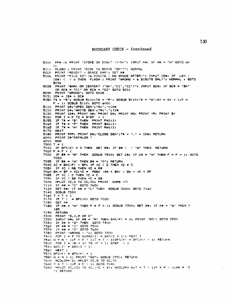
130BOUNDARY CHECK - Continued

5 0 0 0 PR# Os PRINT “STORE ON DISK? <V /N >“ : INPUT AS: IF AS = “N“ GOTO 6 000

5 0 1 0 FLASH s PRINT “DISK IN DRIVE “ DR“^ “ : NORMAL 5 0 2 0 PRINT “READY? - SPACE BAR": GET AS5 0 2 6 PRINT "FILE ID? <6 D IG IT S - NO SPACE AFTER)“ s INPUT IDS: IF LEN (

IDS) < > 6 THEN FLASH s PRINT "WRONG - 6 DIG IT S ONLY": NORMAL : GOTO 5 0 2 6

5 0 2 8 PRINT "BARK OR CENTER? C B K ' , ' C l ' , ' C 2 ' > "x INPUT SCSs IF SCS - "BK"OR SCS ■ "C l" OR SCS - "C2" GOTO 5 0 3 1

5 0 3 0 PRINT "WRONG": GOTO 5 0 2 85 0 3 1 IDS - IDS + SCS5 0 5 0 TS * " S " : GOSUB 5 1 1 0 : T S - " P “ : GOSUB S l l O s T S = "W":BY = BY + 1 : F =

F - 1% GOSUB 5 1 1 0 s GOTO 6 0 0 0 5 1 1 0 PRINT DS;"OPEN D E N " ; T $ ; I D S 5 1 2 0 PRINT DS;"WRITE D E N ' ; T S ; I D S5 1 3 0 PRINT ID S: PRINT NS: PRINT DA: PRINT MO: PRINT YR: PRINT BY5 1 5 0 FOR I - F TO A STEP - 15 1 5 5 IF TS - "S" THEN PRINT FA7. ( I >5 1 6 0 IF TS - "P" THEN PRINT BA7. < I )5 1 6 5 IF TS - "W" THEN PRINT RW7. ( I )5 1 7 0 NEXT5 1 8 0 PRINT 9 9 9 : PRINT DS;"CLOSE DEN"; TS + + ID S: RETURN6 0 0 0 PRINT DS"CATALOG "6 0 1 0 END 7 0 0 0 T - 17 0 1 0 IF BF7.(K) - 0 THEN GET BS: IF BS < > "W" THEN RETURN7 0 2 0 F » F + 17 0 3 0 IF BS ■ "W" THEN GOSUB 7 5 0 0 : GET CS: IF CS - "W" THEN F - F + 1: GOTO

7 0 3 07 0 3 5 IF BS ■ "W" THEN BS » "O": RETURN 7 0 4 0 XC ■ BA7.<F> - S P : IF XC < C THEN XC - C 7 0 5 0 IF XC > RB THEN XC - RB7 0 6 0 BN « SP + XC:YC ■ PEEK <AA + BN) / GN - VC + OF7 0 8 5 IF YC < C THEN YC - C7 0 9 0 IF YC > BB THEN YC * BB7 1 0 0 HPLOT XC,S TO XC,YC: PRINT CHRS (7>7 1 1 0 IF AS - "C" GOTO 7 6 5 07 1 2 0 GET AS: IF AS - "L" THEN GOSUB 3 0 2 0 : GOTO 7 1 6 07 1 4 0 GOSUB 7 3 0 0 7 1 6 0 T = T + 17 1 7 0 IF T < - BF7.(K) GOTO 7 0 2 07 1 8 0 GET AS7 1 8 5 IF AS « "W" THEN F - F 1: GOSUB 7 3 0 0 : GET AS: IF AS = "W“ THEN 7

1 8 57 1 9 0 RETURN7 3 0 0 PRINT “ D , I , M OR C"7 3 2 0 INPUT AS: IF AS * "M" THEN BA7. <F) * O: PRINT “GO": GOTO 2 9 3 07 3 4 0 IF AS ■ "D“ THEN GOTO 7 4 0 07 3 6 0 IF AS * " 1 “ GOTO 7 5 0 07 3 7 0 IF AS = "C" GOTO 7 6 0 07 3 8 0 PRINT "WRONG - “ ; : GOTO 7 3 0 07 4 0 0 FOR I = F TO N:BA7. ( I ) = BA7. ( I + 1 ) : NEXT I7 4 6 0 N = N - 1 : F = F - 1 : T = T - 1:BFV. <K> *= BFV. ( K) - 1: RETURN 7 5 0 0 FOR I « <N ♦ 1) TO <F + 1) STEP - 1 7 5 4 0 BAX ( I > = BA*4 ( I - 1)7 5 6 0 NEXT 17 5 7 0 BF%(K) * BF7. (K) +• 17 5 8 0 N = N + 1: PRINT "GO": GOSUB 2 9 3 0 : RETURN 7 6 0 0 HCOLOR= C: HPLOT XC ,S TO XC,YC 7 6 4 0 T = T - 1 : F = F - 1: GOTO 7 0 4 07 6 5 0 HPLOT XC, 1 3 0 TO XC, (YC 4- 0 ) : HCOLOR= W:T = T - 1 :F * F - 1 : AS = “ Z

“ : RETURhJ

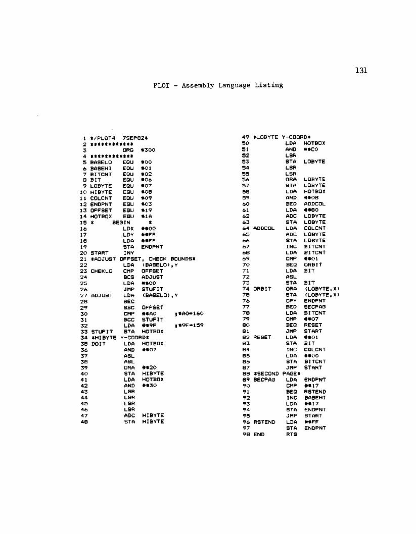
PLOT - Assembly Language Listing

1 $ /P L 0 T 4 7 S E P 8 2 ^ 4 9 ♦LOBYTE Y-COORD^2 * * * * * * * * * * * * 5 0 LDA HOTBOX3 ORG $ 3 0 0 51 AND # $ C 04 * * * * * * * * * * * * 5 2 LSR5 BASELO EQU $ 0 0 5 3 STA LOBYTE6 BASEHI EQU $ 0 1 5 4 LSR7 BITCNT EQU $ 0 2 5 5 LSR8 BIT EQU $ 0 6 5 6 ORA LOBYTE9 LOBYTE EQU $ 0 7 5 7 STA LOBYTE

10 HIBYTE EQU $ 0 8 5 8 LDA HOTBOX11 COLCNT EQU $ 0 9 5 9 AND # $ 0 812 ENDPNT EQU $ 0 3 6 0 BEQ ADDCOL1 3 OFFSET EQU $ 1 9 61 LDA # $ 8 014 HOTBOX EQU $ 1 A 6 2 ADC LOBYTE1 5 * BEGIN ♦ 6 3 STA LOBYTE16 LDX # $ 0 0 6 4 ADDCOL LDA COLCNT17 LDY # $ F F 6 5 ADC LOBYTE18 LDA # $ F F 6 6 STA LOBYTE19 STA ENDPNT 6 7 INC BITCNT2 0 START I NY 6 8 LDA BITCNT21 ♦ADJUST OFFSET, CHECK BOUNDS♦ 6 9 CMP # $ 0 12 2 LDA (BASELO) ,Y 7 0 BEQ ORBIT2 3 CHEKLO CMP OFFSET 71 LDA BIT2 4 BCS ADJUST 7 2 ASL2 5 LDA # $ 0 0 7 3 STA B IT2 6 JMP STUFIT 7 4 ORBIT ORA (LOBYTE,X)2 7 ADJUST LDA (BASELO) ,Y 7 5 STA (LOBYTE,X)2 8 SEC 7 6 CRY ENDPNT2 9 SBC OFFSET 7 7 BEQ SECPAG3 0 CMP # $ A 0 1 $ AO*1 6 0 7 8 LDA BITCNT31 BCC STUFIT 7 9 CMP # $ 0 73 2 LDA # $ 9 F 1 $ 9 F - 1 5 9 8 0 BEQ RESET3 3 STUFIT STA HOTBOX 8 1 JMP START3 4 ♦HIBYTE Y-COORD^ 8 2 RESET LDA # $ 0 13 5 DOIT LDA HOTBOX 8 3 STA B IT3 6 AND # $ 0 7 8 4 INC COLCNT3 7 ASL 8 5 LDA # $ 0 03 8 ASL 8 6 STA BITCNT3 9 ORA # $ 2 0 8 7 JMP START4 0 STA HIBYTE 8 8 ♦SECOND PAGE^41 LDA HOTBOX 8 9 SECPAG LDA ENDPNT4 2 AND # $ 3 0 9 0 CMP # $ 1 74 3 LSR 91 BEQ RSTEND4 4 LSR 9 2 INC BASEHI4 5 LSR 9 3 LDA # $ 1 74 6 LSR 9 4 STA ENDPNT4 7 ADC HIBYTE 9 5 JMP START4 8 STA HIBYTE 9 6 RSTEND LDA # $ F F

9 7 STA ENDPNT9 8 END RTS

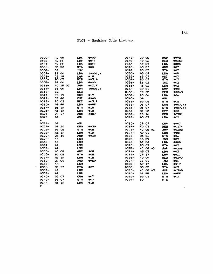
132

0 3 0 0 -0 3 0 2 -0 3 0 4 -0 3 0 6 -0 3 0 8 -0 3 0 9 - 0 3 0 B - 0 3 0 D - 0 3 0 F - 0 3 1 1 - 0 3 1 4 -0 3 1 6 -0 3 1 7 - 0 3 1 9 - 0 3 1 B - 0 3 1 D - 0 3 I F — 0 3 2 1 - 0 3 2 3 -0 3 2 5 - *0 3 2 6 -0 3 2 7 -0 3 2 9 - 0 3 2 B - 0 3 2 D - 0 3 2 F -0 3 3 0 -0 3 3 1 -0 3 3 2 -0 3 3 3 - 0 3 3 5 - 0 3 3 7 -0 3 3 9 - 0 3 3 B - 0 3 3 C - 0 3 3 E - 0 3 3 F -0 3 4 0 - 0 3 4 2 - 0 3 4 4 - *

PLOT - Machine Code Listing

A2 0 0 LDX # $ 0 0 0 3 4 6 - 2 9 0 8 AND # $ 0 8AO FF LDY # $ F F 0 3 4 8 - FO 0 6 BEQ $ 0 3 5 0A9 FF LDA # $ F F 0 3 4 A - A9 8 0 LDA # $ 8 08 5 0 3 STA $ 0 3 0 3 4 C - 6 5 0 7 ADC $ 0 7C8 I NY 0 3 4 E - 8 5 0 7 STA $ 0 7B1 0 0 LDA ( $ 0 0 ) , Y 0 3 5 0 — A5 0 9 LDA $ 0 9C5 1 9 CMP $ 1 9 0 3 5 2 — 6 5 0 7 ADC $ 0 7BO 0 5 BCS $ 0 3 1 4 0 3 5 4 - 8 5 0 7 STA $ 0 7A9 0 0 LDA # $ o o 0 3 5 6 - E6 0 2 INC $ 0 24C IF 0 3 JMP $ 0 3 IF 0 3 5 8 - A5 0 2 LDA $ 0 2B1 0 0 LDA < $ 0 0 > ,Y 0 3 5 A - C9 01 CMP # $ 0 13 8 SEC 0 3 5 C - FO 0 5 BEQ $ 0 3 6 3E5 19 SBC $ 1 9 0 3 5 E - A5 0 6 LDA $ 0 6C9 AO CMP # $ A 0 0 3 6 0 — OA ASL9 0 0 2 BCC $ 0 3 IF 0 3 6 1 — 8 5 0 6 STA $ 0 6A9 9F LDA # $ 9 F 0 3 6 3 — 01 0 7 ORA ( $ 0 7 , X)8 5 1A STA $ 1 A 0 3 6 5 — 81 0 7 STA ( $ 0 7 , X)AS 1A LDA $ 1 A 0 3 6 7 — C4 0 3 CPY $ 0 32 9 0 7 AND # $ 0 7 0 3 6 9 - FO 16 BEQ $ 0 3 8 1OA ASL 0 3 6 B - A5 0 2 LDA $ 0 2

OA ASL 0 3 6 D - C9 0 7 CMP # $ 0 70 9 2 0 ORA # $ 2 0 0 3 6 F — FO 0 3 BEQ $ 0 3 7 48 5 0 8 STA $ 0 8 0 3 7 1 — 4C 0 8 0 3 JMP $ 0 3 0 8AS 1A LDA $ 1 A 0 3 7 4 - A9 01 LDA # $ 0 12 9 3 0 AND # $ 3 0 0 3 7 6 — 8 5 0 6 STA $ 0 64A LSR 0 3 7 8 - E6 0 9 INC $ 0 94A LSR 0 3 7 A— A9 OO LDA # $ 0 04A LSR 0 3 7 C - 8 5 0 2 STA $ 0 24A LSR 0 3 7 E - 4C 0 8 0 3 JMP $ 0 3 0 86 5 0 8 ADC $ 0 8 0 3 8 1 — AS 0 3 LDA $ 0 38 5 0 8 STA $ 0 8 0 3 8 3 - C9 17 CMP # $ 1 7AS 1A LDA $ 1 A 0 3 8 5 - FO 0 9 BEQ $ 0 3 9 02 9 CO AND # $ C 0 0 3 8 7 - E6 01 INC $ 0 14A LSR 0 3 8 9 - A9 17 LDA # $ 1 78 5 0 7 STA $ 0 7 0 3 8 B - 8 5 0 3 STA $ 0 34A LSR 0 3 8 D - 4C 0 8 0 3 JMP $ 0 3 0 84A LSR 0 3 9 0 - A9 FF LDA # $ F F0 5 0 7 ORA $ 0 7 0 3 9 2 - 8 5 0 3 STA $ 0 38 5 0 7 STA $ 0 7 0 3 9 4 - 6 0 RTSA5 1A LDA $ 1 A

133

F * R O G F * A M M A T C H

O E M S I T Y E X I— EE . G M / C C < X 1 O O > (MAXIMUM L ATE WOOD >LIK12B 1852 84 103LIK12B 1860 95 113 105 103LIK12B 1870 86 92 91 89LIK12B 1880 91 85 82 84LIK12B 1890 90 90 84 72LIK12B 1900 92 87 84 66LIK12B 1910 72 79 67 77LIK12B 1920 50 53 62 64LIK12B 1930 52 51 55 45LIK12B 1940 52 61 70 86LIK12B 1950 53 47 49 65LIK12B 1960 49 44 49 71LIK12B 1970 63 43 61 47LIK12B 1980 59 999

89 100 83 103 84 106102 102 89 89 87 8385 86 86 *4 89 7275 87 83 87 94 5292 85 86 85 79 8585 68 68 79 89 8372 49 49 69 61 5163 60 45 65 55 4951 57 42 43 72 6453 59 68 60 56 5760 51 78 67 60 4953 65 56 53 43 6448 52 54 39 53 58

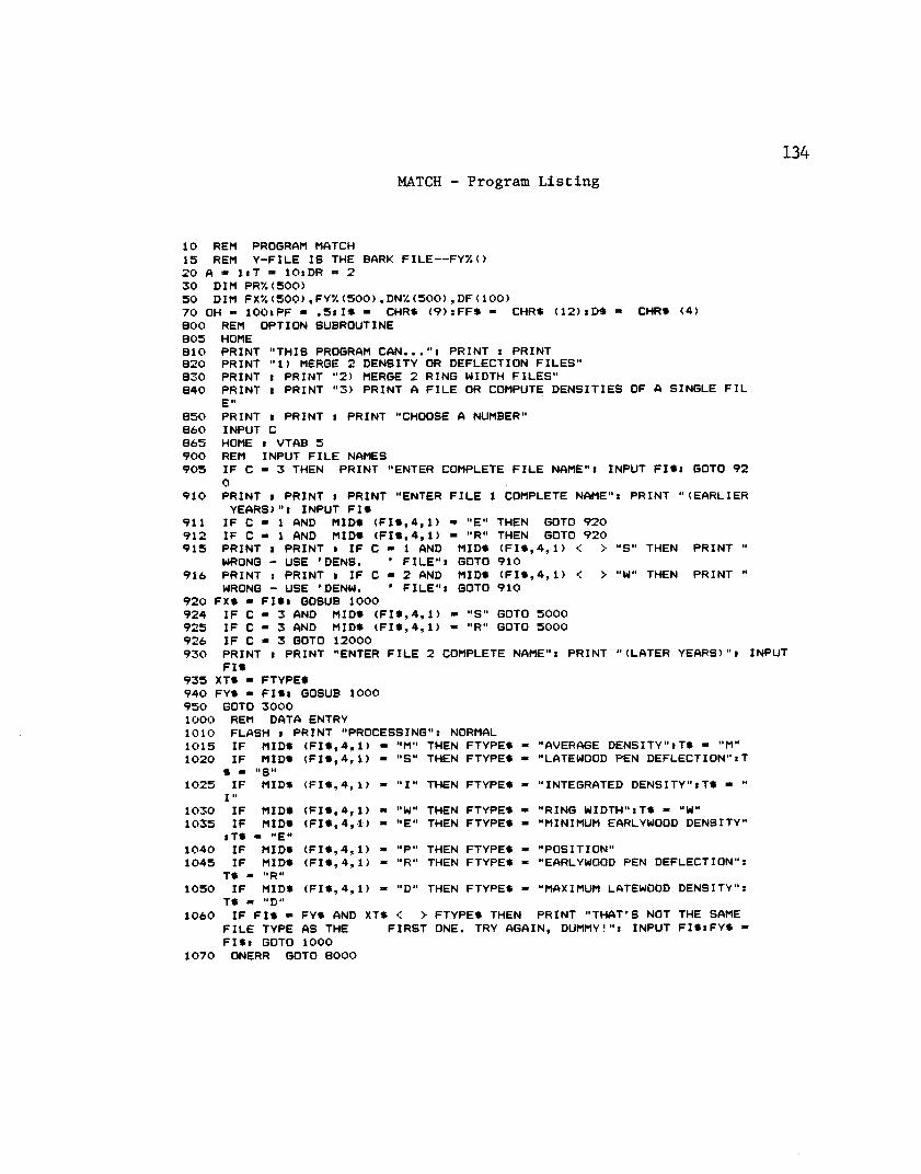
134MATCH - Program Listing

1 0 REM PROGRAM MATCH15 REM Y -F IL E I S THE BARK F IL E — FY7. ( )2 0 A » I s T » 1 0 : DR » 2 3 0 DIM PRY. ( 5 0 0 )5 0 DIM F X % < 5 0 0 ) ,F Y % < 5 0 0 ) ,D N % < 5 0 0 ) , D F ( 100>7 0 OH - 1 0 0 : PF - . 5 : 1 $ « CHRS < 9 > :F F $ ■ CHRS ( 1 2 ) iD S * CHRS ( 4 )8 0 0 REM OPTION SUBROUTINE8 0 5 HOME8 1 0 PRINT "THIS PROGRAM C A N . . . PRI NT : PRINT 8 2 0 PRINT "1> MERGE 2 DENSITY OR DEFLECTION FILES"8 3 0 PRINT : PRINT "2> MERGE 2 RING WIDTH FILES"8 4 0 PRINT : PRINT " 3 ) PRINT A FIL E OR COMPUTE D E N SIT IE S OF A SINGLE FIL

E"8 5 0 PRINT i PRINT i PRINT "CHOOSE A NUMBER"8 6 0 INPUT C8 6 5 HOME : VTAB 59 0 0 REM INPUT FILE NAMES9 0 5 IF C - 3 THEN PRINT "ENTER COMPLETE FIL E NAME": INPUT F I S : GOTO 9 2

09 1 0 PRINT i PRINT : PRINT "ENTER F IL E 1 COMPLETE NAME": PRINT " (EARLIER

YEARS)": INPUT F I S9 1 1 IF C - 1 AND MIDS ( F I S , 4 , 1 ) ■ “E" THEN GOTO 9 2 09 1 2 IF C - 1 AND MIDS ( F I S , 4 , 1 ) ■ "R" THEN GOTO 9 2 09 1 5 PRINT : PRINT i IF C « 1 AND MIDS ( F I S , 4 , 1 ) < > "S" THEN PRINT "

WRONG - USE DENS. ’ F IL E " : GOTO 9 1 09 1 6 PRINT : PRINT i IF C - 2 AND MIDS ( F I S , 4 , 1 ) < > "W" THEN PRINT "

WRONG - USE 'DENW. ' F IL E " : GOTO 9 1 0 9 2 0 FXS - F IS * GOSUB 1 0 0 09 2 4 IF C - 3 AND MIDS ( F I S , 4 , 1 ) - "S" GOTO 5 0 0 09 2 5 IF C * 3 AND MIDS ( F I S , 4 , 1 ) « "R" GOTO 5 0 0 09 2 6 IF C - 3 GOTO 1 2 0 0 09 3 0 PRINT * PRINT "ENTER FIL E 2 COMPLETE NAME": PRINT " (LATER YEARS)":

F I S9 3 5 XTS - FTYPES9 4 0 FYS - F IS * GOSUB 1 0 0 09 5 0 GOTO 3 0 0 01 0 0 0 REM DATA ENTRY1 0 1 0 FLASH : PRINT "PROCESSING": NORMAL1015 IF MIDS (FIS,4, 1) ■ "M" THEN FTYPES - "AVERAGE DENSITY"* TS = "M"1020 IF

$ -MIDS

"S"(FIS,4, 1) * "S" THEN FTYPES ■ "LATEWOOD PEN DEFLECTION":T

1025 IF MIDS (FIS,4, 1) - " I " THEN FTYPES * "INTEGRATED DENSITY":TS - "1030 IF MIDS (FIS,4, 1) * "W" THEN FTYPES ■ "RING WIDTH":T$ • "W"1035 IF

: TSMIDS

m “E"(FIS,4, 1) * "E "

THEN FTYPES * "MINIMUM EARLYWOOD DENSITY"1040 IF MIDS (FIS,4, 1) ■ "P" THEN FTYPES ■ "POSITION"1045 IF

TS -MIDS

« "R"(FIS,4, 1) * " R " THEN FTYPES * "EARLYWOOD PEN DEFLECTION":

1050 IFTS -

MIDS, »D.i (FIS,4, 1) "D" THEN FTYPES ■ "MAXIMUM LATEWOOD DENSITY":1060 IF FIS « FYS AND• XTS < > FTYPES THEN PRINT "THAT'S NOT THE SAME

FIL E TYPE AS THE F IRST ONE. TRY AGAIN, DUMMY!": INPUT F I $ : F Y $ -F IS » GOTO 1 0 0 0

1 0 7 0 ONERR GOTO 8 0 0 0

INPUT

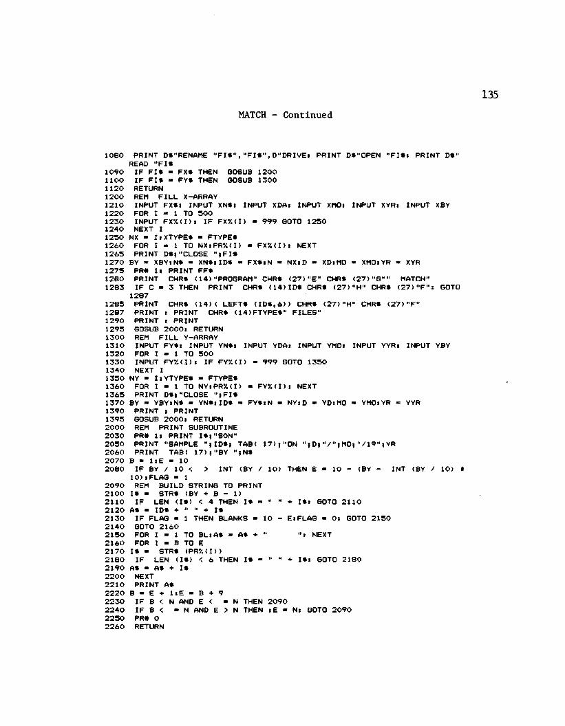
MATCH - Continued

1 0 8 0 PRINT DS"RENAME " F I $ " ," F I $ " ,D " D R I V E * PRINT DS"OPEN " F I $ : PRINT D$" READ " F IS

1 0 9 0 IF F I S = FXS THEN GOSUB 1 2 0 0 1 1 0 0 IF F I S * FYS THEN GOSUB 1 3 0 0 1 1 2 0 RETURN 1 2 0 0 REM FIL L X-ARRAY1 2 1 0 INPUT FXS: INPUT XNS: INPUT XDA: INPUT XMO* INPUT XYRi INPUT XBY1 2 2 0 FOR I ■ 1 TO 5 0 01 2 3 0 INPUT F X % ( I ) : IF FX7.(I> - 9 9 9 GOTO 1 2 5 0 1 2 4 0 NEXT I1 2 5 0 NX - I:XTYPES - FTYPES1 2 6 0 FOR I ■ 1 TO N X :PR % (I) « F X 7 .< I ) i NEXT 1 2 6 5 PRINT DS;"CLOSE " ; F I S1 2 7 0 BY = XBYiNS ■ X N S iID S - F X SiN - NXiD - XDiMO * XMO:YR - XYR 1 2 7 5 PR# l i PRINT FFS1 2 8 0 PRINT CHRS ( 1 4 ) "PROGRAM" CHRS ( 2 7 ) "E" CHRS ( 2 7 ) "G"" MATCH"1 2 8 3 IF C ■ 3 THEN PRINT CHRS ( 1 4 ) IDS CHRS ( 2 7 ) "H" CHRS ( 2 7 ) "F": GOTO

1 2 8 71 2 8 5 PRINT CHRS ( 1 4 ) ( LEFTS ( I D S , 6 ) ) CHRS ( 2 7 ) "H" CHRS ( 2 7 ) "F"1 2 8 7 PRINT : PRINT CHRS ( 1 4 ) FTYPES" FILES"1 2 9 0 PRINT : PRINT 1 2 9 5 GOSUB 2 0 0 0 : RETURN 1 3 0 0 REM FILL Y-ARRAY1 3 1 0 INPUT FYS: INPUT YNSi INPUT YDA: INPUT YMO: INPUT YYRi INPUT YBY1 3 2 0 FOR I » 1 TO 5 0 01 3 3 0 INPUT FY7. ( I ) : IF FY7. ( I ) - 9 9 9 GOTO 1 3 5 0 1 3 4 0 NEXT I1 3 5 0 NY - I iYT Y PE S - FTYPES1 3 6 0 FOR I ■ 1 TO NY :PR % (I) « F Y % (I ) : NEXT 1 3 6 5 PRINT DS;"CLOSE " ; F I S1 3 7 0 BY - YBY:NS - Y N S:ID S * FYS:N - NY:D ■ YD:MO ■ YMO:YR * YYR1 3 9 0 PRINT : PRINT1 3 9 5 GOSUB 2 0 0 0 : RETURN2 0 0 0 REM PRINT SUBROUTINE2 0 3 0 PR# 1: PRINT IS ;"SO N "2 0 5 0 PRINT "SAMPLE " ; ID S; TAB( 1 7 ) ; "ON " | D ; " / " ; MO;" / 1 9 " ; YR 2 0 6 0 PRINT TAB( 1 7 ) ; "BY " ;N $2 0 7 0 B = 1 : E » 102 0 8 0 IF BY / 10 < > INT (BY / 1 0 ) THEN E - 1 0 - (BY - INT (BY / 1 0 ) *

1 0 ) : FLAG = 12 0 9 0 REM BUILD STRING TO PRINT 2 1 0 0 IS - STRS (BY + B - 1)2 1 1 0 IF LEN ( I S ) < 4 THEN I S " + I S : GOTO 2 1 1 02 1 2 0 AS ■ IDS + " " + IS2 1 3 0 IF FLAG « 1 THEN BLANKS - 1 0 - E:FLAG » O: GOTO 2 1 5 0 2 1 4 0 GOTO 2 1 6 02 1 5 0 FOR I - 1 TO BL:AS - AS + " ": NEXT2 1 6 0 FOR I - B TO E 2 1 7 0 IS ■ STRS (PR7.(I> )2 1 8 0 IF LEN ( I S ) < 6 THEN IS " + I S : GOTO 2 1 8 02 1 9 0 AS - AS + IS2 2 0 0 NEXT2 2 1 0 PRINT AS2 2 2 0 B ■ E + 1 iE - B + 92 2 3 0 IF B < N AND E < ■ N THEN 2 0 9 02 2 4 0 IF B < - N AND E > N THEN :E - N: GOTO 2 0 9 02 2 5 0 PR# 02 2 6 0 RETURN

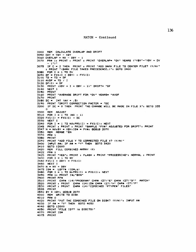
136MATCH - Continued

3 0 0 0 REM CALCULATE OVERLAP AND DRIFT3 0 5 0 DBY ■ YBY - XBY3 0 6 0 OVERLAP * NX - DBY - 13 0 7 0 PR# 1: PRINT i PRINT s PRINT “OVERLAP- "OV” YEARS <"YBY“ - “YBY ♦ OV

- 1 " > "3 0 7 5 IF C - 2 THEN PRINT i PRINT "ADD BARK F ILE TO CENTER F IL E ? < Y /N ) "

i PRINT " (BARK F IL E TAKES PRECEDENCE.) "a GOTO 3 4 0 0 3 0 8 0 FOR I - 1 TO OV 3 0 9 0 DF - FX%(I 4- DBY) - FY7. ( I )3 1 0 0 TD - TD + DF 3 1 1 0 AVDF - TD / I 3 1 2 0 DF <I > - DF3 1 3 0 PRINT (XBY + I + DBY - 1 > “ D R IF T - “DF 3 1 4 0 NEXT I 3 1 5 0 PRINT3 1 6 0 PRINT “AVERAGE DRIFT FOR "OV" YEARS- “AVDF 3 1 7 0 PRINT3 1 8 0 DC - INT (AV + . 5 )3 1 9 0 PRINT "DRIFT CORRECTION FACTOR - "DC3 2 0 0 IF DC - 0 THEN PRINT “NO CHANGE WILL BE MADE IN F ILE X“ i GOTO 3 3 5

O3 3 0 0 REM ADJUST3 3 1 0 FOR I - 1 TO (NX - 1)3 3 2 0 FX7.(I> - FX7.(I> - DC 3 3 3 0 NEXT I3 3 4 0 FOR I - 1 TO NXsPR7.(I> « FX7. ( I > i NEXT3 3 4 5 PRINT i PRINT i PRINT “SAMPLE "FXS" ADJUSTED FOR DR IFT ” 8 PRINT3 3 4 7 N - NXiBY - XBY« ID * - FXSs GOSUB 2 0 7 03 3 5 0 REM MERGE 'EM3 3 7 0 PR# 13 3 8 0 PRINT3 3 9 0 PRINT "ADD F IL E Y TO CORRECTED F ILE X? ( Y / N ) "3 4 0 0 INPUT A S 8 IF AS - "Y" THEN GOTO 3 4 2 0 3 4 1 0 GOTO 1 2 0 0 03 4 2 0 REM FIL L COMBINED ARRAY (X)3 4 2 2 PR# 13 4 2 5 PRINT "YES": PRINT : FLASH 8 PRINT "PROCESSING": NORMAL s PRINT 3 4 3 0 FOR I - 1 TO NY 3 4 4 0 FX7.(I + DBY) - FY7. ( I )3 4 5 0 NEXT I3 4 7 0 N - NY + DBY3 4 7 5 IDS - LEFTS ( I D S , 6 )3 4 8 0 FOR I - 1 TO N:PR%(I> - FX7. ( I ) s NEXT 3 4 9 0 PR# l i PRINT I S ; " 8 0 N "3 5 0 0 PRINT FFS3 5 1 0 PRINT CHRS ( 1 4 ) “PROGRAM" CHRS ( 2 7 ) “E “ CHRS ( 2 7 ) "G“ " MATCH"3 5 2 0 PRINT 8 PRINT CHRS ( 1 4 ) IDS CHRS ( 2 7 ) “H" CHRS ( 2 7 ) "F"3 5 3 0 PRINT s PRINT CHRS ( 1 4 ) “COMBINED “FTYPES" FILES"3 5 3 5 PRINT3 5 4 0 BY - XBY: GOSUB 2 0 7 0 4 0 0 0 REM WRITE TO DISK 4 0 1 0 PR# 04 0 2 0 PRINT "PUT THE COMBINED FIL E ON DISK ? ( Y / N ) " s INPUT AS 4 0 3 0 IF AS - “ Y" THEN GOTO 4 0 5 0 4 0 4 0 GOTO 1 2 0 0 04 0 5 0 PRINT "FILE I D ? ? ( 6 D I G I T S ) "4 0 7 0 PRINT IDS 4 0 7 5 PRINT

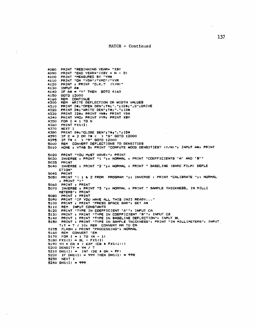
137MATCH - Continued

4 0 8 0 PRINT "BEGINNING YEAR- "XBY 4 0 9 0 PRINT "END YEAR-"(XBY + N - 2 )4 1 0 0 PRINT "MEASURED BY "YN$4 1 1 0 PRINT "ON "YDA" / " YMO" / " YYR 4 1 2 0 PRINT 8 PRINT " O .K .? ( Y / N ) "4 1 3 0 INPUT AS4 1 4 0 IF AS - "Y" THEN GOTO 4 1 6 0 4 1 5 0 GOTO 1 2 0 0 04 1 6 0 REM CONTINUE4 3 0 0 REM WRITE DEFLECTION OR WIDTH VALUES4 3 1 0 PRINT DS;"OPEN D E N " ; T $ ; I D S ; " , D " ; D R I V E4 3 2 0 PRINT DS;"WRITE DEN"; T S ; " . " ; IDS4 3 3 0 PRINT ID S: PRINT YNSs PRINT YDA4 3 4 0 PRINT YMOi PRINT YYRs PRINT XBY4 3 5 0 FOR I - 1 TO N4 3 6 0 PRINT FX7.(I>4 3 7 0 NEXT I4 3 8 0 PRINT DS;"CLOSE DEN"; T S | " . " ; IDS 4 3 9 0 IF C - 2 OR TS < > "S" GOTO 1 2 0 0 0 4 3 9 5 IF TS < > "R" GOTO 1 2 0 0 0 5 0 0 0 REM CONVERT DEFLECTIONS TO DEN SIT IES5 0 1 0 HOME i VTAB 58 PRINT "COMPUTE WOOD D E N SIT IE S? ( Y / N ) " s INPUT AS: PRINT

5 0 2 0 PRINT "YOU MUST HAVE:": PRINT5 0 3 0 INVERSE : PRINT "1 NORMAL : PRINT "COEFFICIENTS ’ A’ AND ' B ' "5 0 3 5 PRINT5 0 4 0 INVERSE 8 PRINT "2 NORMAL 8 PRINT " BASELINE (BARE FILM) DEFLE

CTION"5 0 4 5 PRINT5 0 5 0 PRINT "( 1 & 2 FROM PROGRAM INVERSE : PRINT "CALIBRATE NORMAL

8 PRINT " )"5 0 6 0 PRINT 8 PRINT5 0 7 0 INVERSE : PRINT "3 8 NORMAL 8 PRINT " SAMPLE THICKNESS, IN MILLI

METERS": PRINT 5 0 8 0 PRINT i PRINT5 0 9 0 PRINT " IF YOU HAVE ALL THIS JAZZ R E A D Y . . ."5 1 0 0 PRINT 8 PRINT "PRESS SPACE BAR": GET AS5 1 1 0 REM INPUT CONSTANTS5 1 2 0 PRINT "TYPE IN COEFFICIENT ' A ' ": INPUT CA5 1 3 0 PRINT 8 PRINT "TYPE IN COEFFICIENT ' B ' " : INPUT CB5 1 4 0 PRINT 8 PRINT "TYPE IN BASELINE DEFLECTION": INPUT BL5 1 5 0 PRINT l PRINT "TYPE IN SAMPLE THICKNESS": PRINT "IN MILLIMETERS": INPUT

T :T — T / 108 REM CONVERT MM TO CM 5 1 5 5 FLASH 8 PRINT "PROCESSING"8 NORMAL 5 1 6 0 REM CONVERT 'EM 5 1 7 0 FOR I - 1 TO (N - 1)5 1 8 0 F X 7 .( I ) - BL - F X 7 .( I )5 1 9 0 YH - CA * ( EXP (CB * F X 7 .( I ) ) )5 2 0 0 DENSITY « YH / T5 2 1 0 DN7. ( I ) - I NT (DE * OH + PF)5 2 2 0 IF DN7. ( I ) « 9 9 9 THEN DN7. ( I > - 9 9 8 5 2 3 0 NEXT I 5 2 4 0 DN7. ( I > - 9 9 9

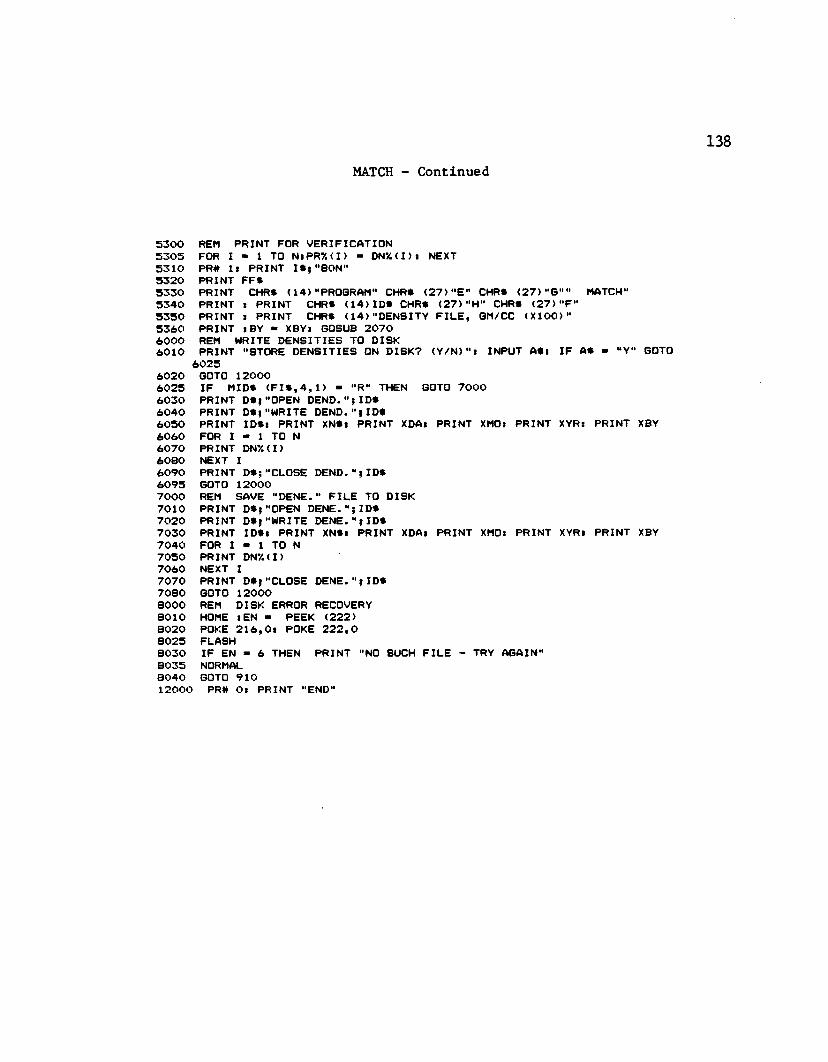
MATCH - Continued

5 3 0 0 REM PRINT FOR VERIFICATION5 3 0 5 FOR I * 1 TO N :P R % (I) - DN%( I ) s NEXT5 3 1 0 PR# 18 PRINT I $ ; " 8 0 N "5 3 2 0 PRINT FFS5 3 3 0 PRINT CHRS ( 1 4 ) "PROGRAM" CHRS ( 2 7 ) "E" CHRS ( 2 7 ) ,,GU" MATCH"5 3 4 0 PRINT i PRINT CHRS ( 1 4 ) IDS CHRS ( 2 7 ) "H" CHRS ( 2 7 ) "F"5 3 5 0 PRINT i PRINT CHRS ( 1 4 ) "DENSITY F IL E , GM/CC ( X 1 0 0 ) "5 3 6 0 PRINT iBY » XBYi GOSUB 2 0 7 0 6 0 0 0 REM WRITE DEN SIT IE S TO DISK6 0 1 0 PRINT "STORE D E N SIT IE S ON DISK ? ( Y / N ) " i INPUT AS: IF AS - “Y" GOTO

6 0 2 56 0 2 0 GOTO 1 2 0 0 06 0 2 5 IF MIDS ( F I S , 4 , 1 ) - "R” THEN GOTO 7 0 0 0 6 0 3 0 PRINT DSj"OPEN D E N D ." ; IDS 6 0 4 0 PRINT DS;"WRITE D E N D ." fID S6 0 5 0 PRINT ID S: PRINT XNSi PRINT XDAi PRINT XMO: PRINT XYR: PRINT XBY 6 0 6 0 FOR I » 1 TO N 6 0 7 0 PRINT DN7. ( I )6 0 8 0 NEXT I6 0 9 0 PRINT DS;"CLOSE D E N D ."?ID S 6 0 9 5 GOTO 1 2 0 0 07 0 0 0 REM SAVE "D E N E ." F IL E TO DISK 7 0 1 0 PRINT DS;"OPEN D E N E ." ? IDS 7 0 2 0 PRINT DS;"WRITE D E N E ." ; IDS7 0 3 0 PRINT ID S: PRINT XNS: PRINT XDA: PRINT XMO: PRINT XYR: PRINT XBY 7 0 4 0 FOR I » 1 TO N 7 0 5 0 PRINT DN7. ( I >7 0 6 0 NEXT I7 0 7 0 PRINT DS;"CLOSE D E N E ." ;I D S 7 0 8 0 GOTO 1 2 0 0 0 8 0 0 0 REM DISK ERROR RECOVERY 8 0 1 0 HOME :EN « PEEK ( 2 2 2 )8 0 2 0 POKE 2 1 6 , 0 : POKE 2 2 2 , 0 8 0 2 5 FLASH8 0 3 0 IF EN ■ 6 THEN PRINT "NO SUCH FILE - TRY AGAIN"8 0 3 5 NORMAL8 0 4 0 GOTO 9 1 01 2 0 0 0 PR# O: PRINT "END"

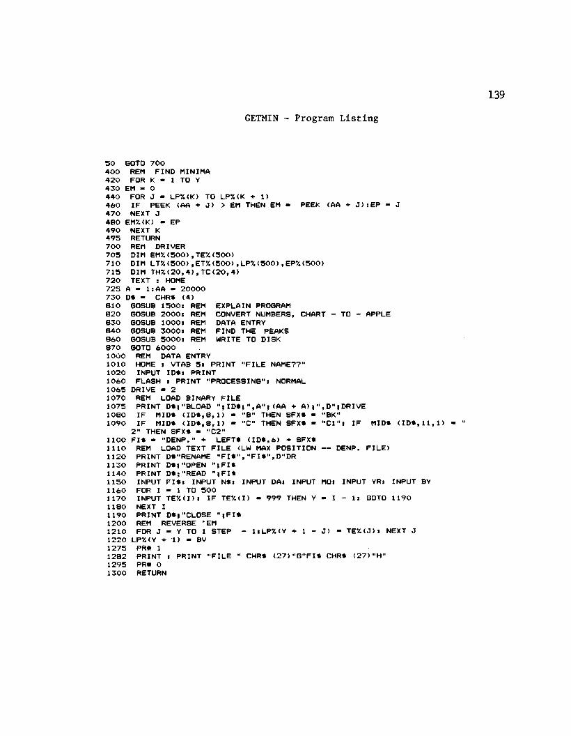
GETMIN - Program L is t in g

50 GOTO 700400 REM FIND MINIMA420 FOR K - 1 TO Y430 EM - 0440 FOR J - LP7.(K> TO LP7.(K + 1)460 IF PEEK (AA + J) > EM THEN EM470 NEXT J

PEEK (AA + J >:EP ■ J480 EM7.(K) - EP 490 NEXT K RETURN

REM DRIVER DIM EM7. (500) , TE7. <500)DIM LT%(500) , ET7. <500) , LP7. (500) , EP7. (500> DIM TH%<20,4),TC(20,4)TEXT s HOME

4957007057107157207257308108208308408608701000101010201060

A ■ 1:AA - 20000 D$ - CHRS <4> GOSUB 1500: REM GOSUB 2000s GOSUB 1000:

EXPLAIN PROGRAMCONVERT NUMBERS, CHART - TODATA ENTRYFIND THE PEAKSWRITE TO DISK

APPLEREM REM

GOSUB 3 0 0 0 : REM GOSUB 5 0 0 0 : REM GOTO 6 0 0 0

REM DATA ENTRYHOME : VTAB 5 : PRINT "FILE NAME??"INPUT ID S: PRINTFLASH i PRINT "PROCESSING": NORMAL

1 0 6 5 DRIVE • 2 1 0 7 0 REM LOAD BINARY FILE

PRINT D$;"BLOAD " ; I D S ; " , A " ; ( A A + A ) ; " ,D " ;D R IV E IF MIDS ( I D S , 8 , 1 ) - "B" THEN SFXS - "BK"IF MIDS ( I D S , 8 , 1 ) ■ "C" THEN SFXS - " C l" : IF

2" THEN SFXS - "C2"F I S - "D E N P ." + LEFTS ( I D S , 6 ) + SFXS

REM LOAD TEXT FILE (LW MAX POSITION — DENP.PRINT DS"RENAME " F I S " , " F I S " , D"DR PRINT DS;"OPEN " ; F I $PRINT DS;"READ " ; F I $INPUT F I S : INPUT NS: INPUT DA: INPUT MO:FOR I - 1 TO 5 0 0INPUT TE7. ( 1 ) : IF TE7. ( I ) - 9 9 9 THEN Y - I - 1: GOTO 1 1 9 0NEXT IPRINT DS;"CLOSE " j F I S REM REVERSE ' EMFOR J - Y TO 1 STEP - 1:LP%(Y + 1 - J ) - T E 7 . ( J ) : NEXT J

1 2 2 0 LP7.(Y + 1) - BV 1 2 7 5 PR# 1

PRINT : PRINT "FILE " CHRS ( 2 7 ) "G "FI$ CHRS ( 2 7 ) "H"PR# 0 RETURN

107510801090110011101120113011401150116011701180119012001210

128212951300

MIDS (IDS,11,1)

FILE)

INPUT YR: INPUT BY

140GETMIN - Continued

1 5 0 0 REM INPUT FIL E INFO1 5 1 0 PRINT 11 YOUR NAME?": INPUT NS1 5 2 0 PRINT "TODAY'S DATE? (D A Y ,M O ,Y R )"1 5 3 0 PRINT "USE NUMBERS - SEPARATE BY"1 5 4 0 PRINT "COMMAS OR 'RE T UR N'": INPUT DA,MO,YR 1 5 5 0 PRINT "BEGINNING YEAR?": INPUT BY 1 5 5 5 PR# 11 5 5 7 PRINT CHRS ( 1 2 )1 5 5 8 PRINT CHRS ( 1 4 ) CHRS ( 2 7 ) "E""PROGRAM " CHRS ( 2 7 ) "G"" GETMIN" CHRS

( 2 7 ) "H" CHRS ( 2 7 ) "F": PRINT1 5 5 9 PRINT CHRS ( 2 7 ) " > " : FOR I ■ 1 TO 5 8 : PRINT CHRS ( 3 5 ) 5 : NEXT I : PRINT

CHRS ( 2 7 ) " * " : PRINT1 5 6 0 PRINT "OPERATOR'S NAME : "NS1 5 6 5 PRINT "TODAY'S DATE : "DA"/"MO"/"YR 1 5 7 0 PRINT "BEGINNING YEAR : "BY 1 5 7 5 PR# 0 1 6 0 0 RETURN2 0 0 0 REM CONVERT CHART NUMBERS TO APPLE NUMBERS 2 1 1 0 PRINT "ENTER LOWER PAIR OF NUMBERS,"2 1 2 0 PRINT 1 PRINT "CHART NUMBER, APPLE NUMBER."2 1 3 0 PRINT "SEPARATE BY COMMA OR RETURN"2 1 4 0 INPUT C 1 ,A 12 1 5 0 PRINT : PRINT "ENTER UPPER P A IR ."2 1 8 0 INPUT C 2 ,A 22 2 0 0 REM COMPUTE LINEAR COEFFICIENTS — A-MSC+B2 2 1 0 DC * C2 - C l : REM DIFF CHART N O 'S2 2 2 0 AD * A2 - A l : REM DIFF APPLE NO 'S2 2 3 0 M - AD / DC: REM SLOPE2 2 4 0 B - A l - M * C l : REM INTERCEPT2 7 7 0 PRINT "CHART VALUE OF HIGHEST PEAK?": INPUT HP2 7 7 5 HP » INT (M * HP + B > : OF - - HP + 102 7 8 0 PRINT "ENTER POINT FROM CHART THAT I S PAST THE "BY" EARLYWOOD MINI

MUM VALUE": INPUT BV 2 7 9 0 RETURN3 0 0 0 REM CONTROL PEAK FINDER 3 0 1 0 PRINT "READY?": GET AS 3 0 2 0 FOR C * 1 TO NS3 0 4 0 I * TH % (C,1) - 1 :E P ■ T H "/.(C ,2):H * TH% (C,3) :L = TH% (C,4)3 0 5 5 FLASH3 0 6 0 PRINT "GOIN' AFTER SECTION "C" , B O S S . "3 0 6 5 NORMAL3 0 8 0 GOSUB 4 0 0 : REM FIND 'EM3 1 0 0 PRINT "DONE — FOUND "Y" MINIMA"3 2 2 0 N * N + (F - N)3 2 4 0 NEXT C 3 3 6 0 RETURN

141GETMIN - Continued

5 0 0 0 PR# O: PRINT "STORE ON DISK? ( Y / N ) " t INPUT AS: IF A$ - "N" GOTO 6 0 0 0

5 0 1 0 FLASH : PRINT "DISK IN DRIVE "DR"?"* NORMAL 5 0 2 0 PRINT "READY? - SPACE BAR": GET AS5 0 2 6 PRINT "FILE ID ? <6 D IG IT S - NO SPACE A F T E R ) I N P U T ID S: IF LEN (

ID S) < > 6 THEN FLASH : PRINT "WRONG - 6 D IG IT S ONLY": NORMAL * GOTO 5 0 2 6

5 0 2 8 PRINT "BARK OR CENTER? C B K ' , ' C l ' , ' C 2 ' ) INPUT SCS: IF SCS - "BK"OR SCS - "C l" OR SCS - "C2" GOTO 5 0 3 1

5 0 3 0 PRINT "WRONG": GOTO 5 0 2 85 0 3 1 IDS * IDS + SCS 5 0 5 0 TS ■ "Q"5 1 1 0 PRINT DS;"OPEN D E N " ; T S ; " . " ; IDS 5 1 2 0 PRINT DS;"WRITE DEN"; T S ; " . " ; IDS5 1 3 0 PRINT ID S: PRINT NS: PRINT DA: PRINT MO: PRINT YR* PRINT BY 5 1 5 0 FOR I - Y TO 1 STEP - 1 5 1 6 0 PRINT EM7. ( I >5 1 7 0 NEXT 5 1 8 0 PRINT 9 9 95 1 9 0 PRINT DS;"CLOSE DEN"; TS + + IDS5 1 9 2 SDS ■ "DENQ." + IDS + " NS"5 1 9 3 PRINT DS;"OPEN "SDS* PRINT DS;"WRITE " ; SDS5 1 9 4 PRINT OF: PRINT NS5 1 9 5 FOR I - 1 TO NS5 1 9 6 FOR J » 1 TO 4 : PRINT TH7. < I , J ) * NEXT J5 1 9 7 NEXT I5 1 9 8 PRINT DS;"CLOSE " ; SDS5 2 0 0 REM WRITE F IL E NAME TO PRINTER5 2 1 0 PRINT : PRINT : PR# 15 2 2 0 PRINT CHRS < 1 4 ) "DATA FOR F IL E "IDS5 2 3 0 PR# 05 2 4 0 RETURN6 0 0 0 REM LOAD BOUNDARY CHECK PROGRAM 6 0 1 0 DRIVE - 16 0 1 5 PRINT "RUN BOUNDARY CHECK PROGRAM? < Y /N >": INPUT AS* IF AS ■ "Y" GOTO

6 0 2 5 6 0 2 0 END6 0 2 5 BCS * "BC-MIN"6 0 3 0 PRINT DS;"RUN " ; B C S ; " , D "; DRIVE

142BOMIN - Program L is t in g

2 0 LOMEM: 3 2 0 0 121 SB - 1 8 UB * 1 2 0 0 0 : GN « 1:M * 2 :N L - 2 4 92 2 A - 1 : BB ■ 1 5 9 : VC - 4 : S ■ 6 : W - 7 :R B * 2 7 9 : AA ■ 2 0 0 0 0 : DR - 22 3 B * 4 82 4 DIM T 7 . ( 1 0 ,4 > :S N « 12 5 DIM FA-/. ( 5 0 0 ) , BA7. (5 0 0 > , RW7. <500> , TE7. ( 5 0 0 ) , BF7. <50)2 8 I S - CHRS ( 9 ) :D S - CHRS ( 4 ) :F F S ■ CHRS ( 1 2 ) sBCS « "BC-MIN"1 0 0 PS - "P L 0T 4": PRINT DS'BLOAD " P $ " ,D " 1 3 9 0 HOME i VTAB 54 0 0 PRINT "FILE NAME?": INPUT F I S : I D S ■ "DENQ." + LEFTS ( F I S , 6 ) 4- "BK"

: IF MIDS ( F I S , 8 , 1 ) - "C" THEN IDS - LEFTS ( I D S , 1 1 ) + "C l"5 0 2 FLASH : PRINT "PROCESSING": NORMAL 5 0 5 PRINT DS"RENAME " I D S " , " I D S " , D"DR 5 1 0 PRINT DS;"OPEN " ; IDS 5 1 5 PRINT DS;"READ " ; IDS5 2 0 INPUT DDS: INPUT NS: INPUT DA: INPUT MO: INPUT YR: INPUT BY 5 3 0 FOR I - 1 TO 5 0 05 4 0 INPUT TE7. ( I > : IF TE7.( I > - 9 9 9 THEN N ■ I : GOTO 5 6 0 5 5 0 NEXT I5 6 0 PRINT DS;"CLOSE " ; IDS5 7 0 FOR J - (N - 1 ) TO 1 STEP - 1:BA%(N - J> ■ TE 7.(J) : NEXT J:BA% (N) •

9 9 96 0 0 SDS = IDS + " NS"6 1 0 PRINT DS;"OPEN " ; SDS 6 2 0 PRINT DS;"READ " ; SDS 6 3 0 INPUT OF: INPUT NS6 4 0 FOR SN « 1 TO NS: INPUT T % (S N ,1 ) : INPUT T7.(SNf 2 > : INPUT T7.(SN, 3 ) : INPUT

T % ( S N , 4 ) : NEXT6 7 0 PRINT DS;"CLOSE " ; S D $ : S N - 1 7 2 0 FOR Q - 1 TO B 7 3 0 SP - (Q - 1) * 2 5 0 + 1:W - O 7 4 0 F " F + 1 : W * W + 17 5 0 IF BA7.(F) ■ 9 9 9 THEN F - O: GOTO 1 0 1 07 6 0 IF BA%(F) < 2 5 0 4- SP THEN BF7.(Q) - W: GOTO 7 4 07 7 0 F - F - 17 8 0 NEXT Q1 0 1 0 PRINT "BLK # ? " : INPUT SB1 0 6 0 PRINT "READY?": GET AS: FLASH : PRINT "PROCESSING": NORMAL

BC-MIN - Continued

1 0 7 0 FOR I - 0 TO (SB - 1 ) : F - F + BF7. ( I ) $ NEXT I 1 1 1 0 PRINT DS"BLOAD " F I S " , AM<AA + 1 ) ",D"DR 2 2 5 0 W * 7 : K - SB: PR# Is PRINT FFS2 2 6 0 TEXT s HOME : HGR sS P - <K - 1> * 2 5 0 + l ; E P - SP + RBi IF K - B THEN

EP - UB2 5 0 5 VTAB 2 1 * PRINT F I S S P C < 8 ) "BLK # "K2 5 1 6 HS « 0% FOR I » 1 TO 2 8 : HPLOT H S , 0 TO H S , 2 : H S - HS 10* NEXT I 2 5 2 1 HS ■ Os FOR I - 1 TO 6 s HPLOT H S , 0 TO H S ,5 * H S - HS + 5 0 * NEXT I 2 5 5 0 HPLOT 2 5 0 , 0 TO 2 5 0 , 1 02 6 1 0 P « 0 : IF K / 2 - I NT (K / 2 ) THEN P - 5 02 6 2 0 Q « P + 2 0 0 s FOR I - P TO Q STEP 1 0 0 s HPLOT 1 , 1 5 5 TO 1 , 1 5 0 : NEXT I2 6 4 0 HB - INT ( <SP + AA) / 2 5 6 ) sLB « (SP + AA) - HB * 2 5 6 s POKE 0 ,L B s POKE

1 , HB: POKE 2 , 0 s POKE 6 , 1 s POKE 7 , 0 s POKE 8 , 0 * POKE 9 , 0 * POKE 2 5 , - OFs CALL 7 6 8

2 7 0 0 IF SN > NS THEN 2 7 7 12 7 0 5 IF T% (SN,1> < - SP THEN SX - 02 7 1 0 IF T% < S N ,1) > SP THEN SX - T % (S N ,1 ) - S P : IF SX > RB THEN SX ■ RB 2 7 3 0 IF TV, (SN , 2 ) > - EP THEN EX - RB2 7 4 0 IF T % (S N ,2 ) < - EP THEN EX - T % (S N ,2 ) - SP*SC - I s IF EX < C THEN

EX « C2 7 5 0 YL - TV, (SN , 3 ) + OF* YE - T% (SN,4> + OF 2 7 6 0 HPLOT SX ,Y L TO EX,YL* HPLOT SX ,Y E TO EX,YE2 7 7 0 IF SC - 1 THEN SN « SN *»- 1*SC « O* GOTO 2 7 0 02 7 7 1 GOSUB 7 0 0 0 s GOTO 3 2 0 0 2 8 9 0 BN - SP + XC2 8 9 2 IF F - O GOTO 2 9 0 02 8 9 5 IF BN < - BA7.(F - 1 ) THEN D - I s GOTO 2 9 8 02 9 0 0 YC - PEEK (AA + BN) / GN - VC + OF2 9 1 0 IF YC < C THEN YC - C2 9 1 2 IF YC > BB THEN YC - BB2 9 2 0 HPLOT X C ,S TO XC, YC2 9 3 0 GET AS* IF AS - "K" THEN D - 1* GOTO 2 9 6 0 2 9 3 5 IF AS - "J" THEN D ■ - 1: GOTO 2 9 6 02 9 4 0 IF AS - "R" THEN GOSUB 3 0 0 5 * RETURN2 9 4 7 PRINT "WRONG - "* GOTO 2 9 3 0 2 9 6 0 HCOLOR- C: HPLOT X C ,S TO XC,YC* HCOLOR- W 2 9 8 0 XC - XC + D2 9 8 5 IF XC > RB THEN XC - RB: GOTO 3 2 0 0 2 9 8 7 IF XC < C THEN XC - C 2 9 9 0 GOTO 2 8 9 03 0 0 5 IF BN - BA7.(F> THEN RETURN3 0 0 7 BA7.(F) - BN3 0 1 7 IF BA7.(F> - 9 9 9 THEN BA7.(F> - 9 9 8 3 0 2 0 FA7.(F) » PEEK (AA + BN) s PRINT CHRS ( 7 )3 0 2 5 HPLOT X C ,1 3 0 TO XC ,(Y C + 8 )3 0 2 7 IF YY ■ O THEN PRINT "YEAR ?"* INPUT YY3 0 2 9 PR# Is PRINT YY" AT PT "BN" I S " PEEK (AA + B N ): PR# OsYY - YY - 1

% RETURN 3 2 0 0 K » K + 1 3 2 1 0 IF K < • B GOTO 2 2 6 03 4 2 0 FOR I - 1 TO (F - 1 > s RW7. ( I ) - (BA7.(I + 1) - BA7. ( I ) > t Ms NEXT I 4 0 0 0 TEXT s PRINT "PRINT RESULTS? ( Y / N ) ": INPUT AS* IF AS - "N" GOTO 6 0

0 04 0 0 6 PR# I s PRINT CHRS ( 1 2 ) CHRS ( 1 4 ) F I S4 0 0 9 PRINT * PRINT CHRS (1 4 ) B C S s PRINT4 0 1 0 PRINT "YEAR" TAB( 1 5 ) "WIDTH" TAB( 2 4 ) "DEF" TAB( 3 3 ) "PT"* PRINT 4 0 1 3 BY » YY + 14 0 2 0 FOR J ■ F TO 1 STEP - 14 0 2 5 YY « YY + Is PRINT YY TAB( 15)RW%(J) TAB( 2 4 )F A % (J ) TAB( 3 3 )B A % (J )4 0 3 0 NEXT J

144BC-MIN - Continued

5 0 0 0 PR# Oi PRINT “STORE ON DISK ? <Y /N >" t INPUT A S 8 IF AS - “N ” GOTO 6 0 0 0

5 0 1 0 FLASH i PRINT "DISK IN DRIVE “DR“? “ % NORMAL 5 0 2 0 PRINT "READY? - SPACE BAR": GET AS5 0 2 6 PRINT "FILE ID « "IDS" ? ( Y /N ) " x INPUT AS: IF AS - "Y" THEN IDS *

FLIGHTS ( I D S , 8 ) : GOTO 5 0 5 05 0 2 8 PRINT "FILE ID ? <6 D IG IT S - NO SPACE AFTER)": INPUT ID S: IF LEN <

ID S) < > 6 THEN FLASH x PRINT "WRONG - 6 D IG IT S ONLY": NORMAL : GOTO 5 0 2 8

5 0 3 0 PRINT "BARK OR CENTER? C B K ' , ' C l ' , ' C 2 ' >": INPUT SCS: IF SCS - "BK"OR SCS - "C l" OR SCS - "C2" GOTO 5 0 3 4

5 0 3 2 PRINT "WRONG": GOTO 5 0 3 0 5 0 3 4 IDS ■ IDS + SCS5 0 5 0 TS • "R” : GOSUB S l l O x T S ■ "Q": GOSUB 5 1 1 0 : GOTO 6 0 0 0 5 1 1 0 PRINT DS;"OPEN D E N " ; T $ ; I D S 5 1 2 0 PRINT DS;"WRITE D E N " ; T S ; I D S5 1 3 0 PRINT ID S: PRINT NS: PRINT DA: PRINT MO: PRINT YR: PRINT BY5 1 5 0 FOR I - F TO A STEP - 15 1 5 5 IF TS - "R" THEN PRINT FA7. < I >5 1 6 0 IF TS - "Q" THEN PRINT BA7. ( I >5 1 7 0 NEXT5 1 8 0 PRINT 9 9 9 : PRINT DS;"CLOSE DEN"; TS + " . " ♦ ID S: RETURN 6 0 0 0 PRINT DS"CATALOG "6 0 1 0 END 7 0 0 0 T - 17 0 1 0 IF BF7.(K) - 0 THEN GET BS: IF BS < > "W" THEN RETURN7 0 2 0 F - F + 17 0 3 0 IF BS - "W" THEN GOSUB 7 5 0 0 : GET CS: IF CS - "W" THEN F - F + 1 i GOTO

7 0 3 07 0 3 5 IF BS - "W" THEN BS - "O": RETURN 7 0 4 0 XC - BA/C(F) - S P : IF XC < C THEN XC - C 7 0 5 0 IF XC > RB THEN XC - RB 7 0 6 0 BN - SP + XC7 0 8 0 YC - PEEK (AA + BN) / GN - VC + OF7 0 8 5 IF YC < C THEN YC - C7 0 9 0 IF YC > BB THEN YC ■ BB7 1 0 0 HPLOT X C ,S TO XC,YC: PRINT CHRS ( 7 )7 1 1 0 IF AS = "C" GOTO 7 6 5 07 1 2 0 GET AS: IF AS ■ "L" THEN GOSUB 3 0 2 0 : GOTO 7 1 6 0 7 1 4 0 GOSUB 7 3 0 0 7 1 6 0 T - T + 17 1 7 0 IF T < « BF7.<K> GOTO 7 0 2 07 1 8 0 GET AS7 1 8 5 IF AS ■ "W" THEN F » F + 1: GOSUB 7 3 0 0 : GET AS: IF AS - "W" THEN 7

1 8 57 1 9 0 RETURN7 3 0 0 PRINT " D , I , M OR C"7 3 2 0 INPUT AS: IF AS - "M" THEN BA7.<F> - Or PRINT "GO": GOTO 2 9 3 07 3 4 0 IF AS - "D" THEN GOTO 7 4 0 07 3 6 0 IF AS - " I" GOTO 7 5 0 07 3 7 0 IF AS ■ "C" GOTO 7 6 0 07 3 8 0 PRINT "WRONG - " ;» GOTO 7 3 0 07 4 0 0 FOR I - F TO N:BA% <I ) ■ BAX <I + 1 ) : NEXT I7 4 6 0 N » N - 1 : F ■ F - l i T ■ T - 1 :B F X (K ) ■ BFX(K) - 1: RETURN7 5 0 0 FOR I - (N + 1) TO (F + 1) STEP - 17 5 4 0 BAX <I ) - BAX (I - 1)7 5 6 0 NEXT I7 5 7 0 BFX(K) - BFX(K) + 17 5 8 0 N » N ♦ 1: PRINT "GO": GOSUB 2 9 3 0 : RETURN 7 6 0 0 HCOLOR- C: HPLOT X C ,S TO XC,YC 7 6 4 0 T - T - 1 : F » F - 1 : GOTO 7 0 4 07 6 5 0 HPLOT X C ,1 3 0 TO XC, (YC + 8 ) : HCOLOR- WiT - T - 1 : F - F - lx AS - "Z

": RETURN

AVDEN - Program L is t in g

10 REM 'GRAM TO COMPUTE AVERAGE DEN SIT IE S 2 0 REM AND INTEGRATED DEN SIT IE S 3 0 REM OVER PORTIONS OF A CORE (MANUAL)4 0 REM OR FOR THE WHOLE CORE (AUTO)5 0 D$ « CHRS ( 4 )6 0 DIM T E % ( 5 0 0 ) ,B A % ( 5 0 0 > ,A V % ( 5 0 0 ) , IA % (5 0 0 )7 0 A ■ 1*AA - 2 0 0 0 0 s DR - 2 : 0 H « 1 0 0 s P F » , 5 s TWO - 2 1 0 0 REM DRIVER1 1 0 HOME s VTAB 5 s PRINT "WANT TO COMPUTE AVERAGE DENSITY “ s PRINT "AND

INTEGRATED DENSITY FOR s "1 2 0 PRINT s PRINT s PRINT " 1 ) PART OF A CORE": PRINT "2) THE WHOLE CORE

1 3 0 PRINT s PRINT s PRINT "CHOOSE 1 OR 2 " i INPUT Ds GOSUB 4 0 0 1 3 5 GOSUB 6 0 01 4 0 IF D - 1 THEN GOSUB 7 0 01 5 0 IF D - 2 THEN GOSUB 2 0 01 6 0 GOSUB 5 0 0 01 7 0 PRINT s PRINT "THAT'S IT JACK!"1 8 0 GOTO 6 0 1 02 0 0 REM COMPUTE AVERAGE D E N SIT IE S FOR RINGS2 0 5 FLASH 8 PRINT "COMPUTING": NORMAL 2 1 0 FOR I - 1 TO (N - 2 )2 2 0 NR « BA7. ( I + 1) - BA% ( I ) s SUM - 0 2 3 0 FOR K - BA7. ( I ) TO (BA%(I 4- 1 ) - 1)2 4 5 SG - (A S EXP (B * (BL - PEEK (AA + K ) ) ) > / TsSUM - SUM + SG2 5 0 NEXT K2 5 5 AV - SUM / NR2 6 0 AV%(I) - INT (AV * OH + PF)2 6 5 IA - SUM * TWO:IA%(I) - INT ( I A + PF)2 7 0 NEXT I 2 8 0 RETURN4 0 0 PRINT "FILE NAME?"s INPUT F I S b IDS - " D E N P ." + LEFTS ( F I S , 6 ) + "BK"

8 IF MIDS ( F I S , 8 , 1 ) - "C" THEN IDS - LEFTS ( I D S , 1 1 ) + "C l"5 0 0 FLASH : PRINT "PROCESSING": NORMAL5 0 2 PRINT DSs"BLOAD " j F I S | " , A"j (AA + A ) ; " ,D " ;D R5 0 5 PRINT DS"RENAME " I D S " , " I D S " , D"DR5 1 0 PRINT DS;"OPEN " ; IDS5 1 5 PRINT DS;"READ " ; IDS5 2 0 INPUT DOS: INPUT NS: INPUT DA: INPUT MO: INPUT YR: INPUT BY5 2 5 BY - BY 4- 15 3 0 FOR I - 1 TO 5 0 05 4 0 INPUT T E % (I ) : IF TE% (I) - 9 9 9 THEN N - I : GOTO 5 6 0 5 5 0 NEXT I5 6 0 PRINT DS:"CLOSE “ | I D S5 7 0 FOR J - (N - 1) TO 1 STEP - 1:BA%(N - J ) - T E % (J ): NEXT J:BA%(N> «

9 9 95 8 0 RETURN

146AVDEN - Continued

6 0 0 REM ENTER CONSTANTS6 1 0 PRINT i PRINT "NOW YOU NEED DATA FROM"6 1 5 PRINT "PROGRAM INVERSE 3 PRINT "CALIBRATE": NORMAL6 2 0 PRINT i PRINT "ENTER COEFFICIENT ’ A’ . "6 3 0 INPUT A6 4 0 PRINT % PRINT "ENTER COEFFICIENT ' B ' . "6 5 0 INPUT B6 6 0 PRINT i PRINT "ENTER BASELINE DEFLECTION."6 7 0 INPUT BL6 8 0 PRINT "ENTER SPECIMEN THICKNESS ( IN MM AS FOUND ON CALIBRATE PRINT

OUT)6 9 0 INPUT T iT * T / 1 0 6 9 5 RETURN7 0 0 REM MANUAL COMPUTATIONAL ROUTINE7 2 0 REM S B -S P E C IF IC GRAVITY (DENSITY) ------ T - THICKNESS, CM7 3 0 PR# 1: PRINT CHRS ( 1 4 ) CHRS ( 2 7 ) "E" CHRS ( 2 7 ) "G"" " F IS CHRS ( 2 7

) "F" CHRS ( 2 7 ) "H": PR# O 7 3 5 PR# I s PRINT i PRINT » PRINT i PR# 0 7 4 0 PRINT "AVERAGE DENSITY WILL BE COMPUTED"7 4 5 PRINT "FROM LOWER BOUND INCLUSIVE TO"7 5 0 PRINT "UPPER BOUND EXCLUSIVE": PRINT I PRINT7 6 0 PRINT "ENTER LOWER BOUND ------ ’ Q’ TO QUIT": INPUT L S iL B - VAL (L S)7 7 0 IF LS - "Q" THEN HOME « GOTO 1 7 07 8 0 PRINT "ENTER UPPER BOUND” i INPUT UB8 0 0 NR • UB - LBiSUM - O8 1 0 PR# 1* PRINT "LOWER BOUND - "LB8 2 0 PRINT "UPPER BOUND - "UB8 3 0 PR# 08 5 0 FOR K - LB TO (UB - 1)8 6 0 SG - (A * EXP (B * (BL - PEEK (AA ♦ K ) ) ) ) / TsSUM - SUM + SG8 7 0 NEXT K8 8 0 AV - SUM / NR8 8 5 PL - 1 0 0 08 9 0 RA - INT (AV * PL + P F) / PL9 0 0 PR# I s PRINT i PRINT "AVERAGE DENSITY - "RA" GRAMS/CC": PRINT i PRINT

i PR# O 9 2 0 GOTO 7 6 05 0 0 0 PR# Os PRINT "STORE ON DISK? ( Y / N ) " i INPUT AS: IF AS - "N" GOTO 6 0005 0 1 0 FLASH s PRINT "DISK IN DRIVE "DR"?": NORMAL 5 0 2 0 PRINT "READY? - SPACE BAR": GET AS5 0 2 6 PRINT "FILE ID - "IDS" ? ( Y / N ) " : INPUT AS: IF AS - "Y" THEN IDS -

RIGHTS ( I D S , 8 ) s GOTO 5 0 5 05 0 2 8 PRINT "FILE ID ? ( 6 D IG IT S - NO SPACE AFTER)": INPUT ID S: IF LEN (

ID S) < > 6 THEN FLASH : PRINT "WRONG - 6 D IG IT S ONLY": NORMAL : GOTO 5 0 2 8

5 0 3 0 PRINT "BARK OR CENTER? ( ’ BK’ , ’ C l ’ , ’ C 2 ’ ) " : INPUT SCS: IF SCS - "BK"OR SCS - "C l" OR SCS - "C2" GOTO 5 0 3 4

5 0 3 2 PRINT "WRONG": GOTO 5 0 3 0 5 0 3 4 IDS - ID * + SCS5 0 5 0 TS - "M": GOSUB S l l O t T S - " I " : GOSUB 5 1 1 0 : GOTO 6 0 0 0 5 1 1 0 PRINT DSj"OPEN D E N " ; T S ; I D S 5 1 2 0 PRINT DS;"WRITE DEN"$T S | " . " | I D S5 1 3 0 PRINT ID S: PRINT NS: PRINT DA: PRINT MO: PRINT YR: PRINT BY5 1 5 0 FOR I - (N - 2 ) TO 1 STEP - 15 1 5 5 IF TS - "M" THEN PRINT AV7. ( I >5 1 6 0 IF TS - " I" THEN PRINT IA%(I>5 1 7 0 NEXT5 1 8 0 PRINT 9 9 9 : PRINT DS;"CLOSE DEN";TS + " + ID S : RETURN6 0 0 0 PRINT DS"CATALOG "6 0 1 0 END

LIST OF REFERENCES

Chemical Rubber Publishing Co.1961 Handbook of Chemistry and Physics, 43rd Ed. Chemical Rubber Publishing Co.,Cleaveland. 3513 p.

Clague, J., L. A. Jozsa, and M. L. Parker1982 Dendrochronological dating of glacier-dammedlakes: an example from Yukon Territory, Canada. Arctic and Alpine Research 14: 301-310.

Cleaveland, M. K.1975 Dendroclimatic relationships of shortleaf pine

( Pinus eehinata ) in the South Carolina Piedmont. M. S. Thesis, Clemson University, Clemson. South Carolina. 189 p.

1983 X-ray densitometric measurements of climaticinfluence on the intra-annual characteristics of southwestern semiarid conifer tree-rings. PhD Dissertation, University of Arizona, Tucson, Arizona, 177 p.

Conkey, L. 1979

E.Response of tree-ring density to climate in Maine, U.S.A. Tree-Ring Bulletin 39: 29-38.

1983 Eastern U.S. Tree-Ring Widths and Densities as Indicators of Past Climate. PhD Dissertation, University of Arizona, Tucson, Arizona. 204 p.

Coughlin,1977

R. F., and F. F. Driscoll Operational Amplifiers and Linear Integrated Circuits! Prentice-Hall, Englewood Cliffs. 312 p.

Daniels, F., and R. A. Alberty1975 Physical Chemistry. John Wiley and Sons,

New York. 687 p.Eastman Kodak Company

1969 Radiography in Modern Industry. Eastman Kodak Co., Rochester. 160 p.

147

148Echols, R. M.

1970 Moving-slit radiography of wood samples forincremental measurements. In "Tree-ring Analysis with Special Reference to North America," Smith and worrall, Eds. University of British Columbia Faculty of Forestry Bulletin 7: 34-36.

1972 Patterns of wood density distribution and growth rate in ponderosa pine. Proc. Symp. on Effect of Growth Acceleration on Properties of Wood. Forest Products Lab., Madison, Wisconsin, H1-H18.

1973 Uniformity of wood density assessed from X-rays of increment cores. Wood Science and Technology 7: 34-44.

Evertson, J. A.1982 Inter-laboratory standardization survey. Wood Microdensitometry Bulletin 2(2): 3-24.

Fletcher, J. M., and J. F. Hughes1970 Uses of X-rays for density determinations and

dendrochronology. In "Tree-ring Analysis with Special Reference to North America," Smith and Worral, Eds. University of British Columbia Faculty of Forestry Bulletin 7: 41-54.

Hewlett-Packard Company1975 HP-25 Applications Programs. Hewlett-Packard Co.,

Cupertino. 161 p.Jones, F.

1970W., and M. L. ParkerG. S. C. tree-ring scanning densitometer and data acquisition system. Tree-Ring Bulletin 30: 23-31.

Kusec, D. 1972

J.Twin-blade saw for precision machining of increment cores. Wood and Fiber 4(1): 44-49.

Lenz, 0.1957 Utilisation de la radiographie pour I'examen des couches d'accroissement. Institut Suisse de Reserches Forestieres 33(5): 125-134.

Lenz, 0., E. Schar, and F. H. Schweingruber1976 Methodische Probleme bei der radiographisch-

densitometrischen Bestimmung der Dichte und der Jahrringbreiten von Holz.Holzforschung 30: 114-123.

149

Olson, J. R., D. G. Arganbright, and P. T. Rygiewicz1978 Increment core planar for X-ray densitometric

sample preparation. Wood Science 11(1): 33-36.Parker, M.

1976L.Improving tree-ring dating in northern Canada by X-ray densitometry. Syesis 9: 163-172.

Parker, M. L., and W. E. S. Henoch1971 The Use of Engelmann Spruce Latewood Density for

Dendrochronological Purposes. Canadian Journal of Forest Research 1: 90-98.

Parker, M. L., and K. R. Meleskie1970 Preparation of X-ray negatives of tree-ring

specimens for dendrochronological analysis. Tree-Ring Bulletin 30; 11-22.

Polge, H.1965 Study of wood density variations by densitometric

analysis of X-ray negatives of samples taken with a pressler auger. Paper presented to a meeting of I.U.F.R.O. ( Section 41), October, 1965.

1966 Etablissement des courbes de variation de ladensite du bois par exploration densitometrique de radiographies d'echantillons preleves a la tariere sur des arbres vivants. Application dans les domaines technologique et physiologique. Annales des Sciences Forestieres 23: 1-206.

Polge, H., 1972

and J. W. P. NichollsQuantitative radiography and the densitometric analysis of wood. Wood Science 5(1): 51-59.

RCA Corporation1970 Photomultiplier Manual. RCA Corporation,

Harrison, New Jersey.Rudman, P.

1968 Growth Ring Analysis. Journal of the Institute of Wood Science 4(2): 58-63.

1969 Quantitative determination of wood density byX-ray densitometry. Journal of the Institute of Wood Science 4(6): 37-43.

Schweingruber, F. H.1979 Personal communication. Swiss Forest Research

Institute, Birmensdorf, Switzerland.

150Schweingruber, F. H., H. C. Fritts, 0. D. Braker,L. G. Drew, E. Schar

1978 The X-ray Technique as Applied toDendroclimatology", Tree-Ring Bulletin 38: 61-91.

Sears, F. W., and M. W. Zemansky1964 University Physics. Addison-Wesley,

Reading. 1023 p.Skoog, D. A., and D. M. West

1974 Analytical Chemistry. Holt, Rinehart, andWinston, New York. 598 p.

Shigley, J. E.1963 Mechanical Engineering Design. McGraw-Hill,

New York. 631 p.Stokes, M. A., and Smiley, T. L.1968 An Introduction to Tree-Ring Dating. University

of Chicago Press, Chicago. 73 p.Telewski,

1982F. W.Personal communication.

Telewski, F. W., A. H. Wakefield, and M. J. Jaffe1982 Computer assisted image analysis of tissues of

ethrel treated Pinus taeda seedlings. Unpublished manuscript.

Wallis, A. W., and Roberts, H. V.1956 Statistics: A New Approach. The Free Press,

Glencoe, Illinois. 646 p.