© 2020. This manuscript version is made available under the CC-BY-NC-ND 4.0 license http://creativecommons.org/licenses/by-nc-nd/4.0/

A New Validity Index for Fuzzy-Possibilistic C-Means Clustering

𝑀𝑜ℎ𝑎𝑚𝑚𝑎𝑑 𝐻𝑜𝑠𝑠𝑒𝑖𝑛 𝐹𝑎𝑧𝑒𝑙 𝑍𝑎𝑟𝑎𝑛𝑑𝑖𝑎,∗ , 𝑆ℎ𝑎ℎ𝑎𝑏𝑒𝑑𝑑𝑖𝑛 𝑆𝑜𝑡𝑢𝑑𝑖𝑎𝑛𝑎 , 𝑂𝑠𝑐𝑎𝑟 𝐶𝑎𝑠𝑡𝑖𝑙𝑙𝑜𝑏

𝐷𝑒𝑝𝑎𝑟𝑡𝑚𝑒𝑛𝑡 𝑎 𝑜𝑓 𝐼𝑛𝑑𝑢𝑠𝑡𝑟𝑖𝑎𝑙 𝐸𝑛𝑔𝑖𝑛𝑒𝑒𝑟𝑖𝑛𝑔 𝑎𝑛𝑑 𝑀𝑎𝑛𝑎𝑔𝑒𝑚𝑒𝑛𝑡 𝑆𝑦𝑠𝑡𝑒𝑚𝑠, 𝐴𝑚𝑖𝑟𝑘𝑎𝑏𝑖𝑟 𝑈𝑛𝑖𝑣𝑒𝑟𝑠𝑖𝑡𝑦 𝑜𝑓 𝑇𝑒𝑐ℎ𝑛𝑜𝑙𝑜𝑔𝑦, 𝑇𝑒ℎ𝑟𝑎𝑛, 𝐼𝑟𝑎𝑛

𝑇𝑖𝑗𝑢𝑎𝑛𝑎 𝑏 𝐼𝑛𝑠𝑡𝑖𝑡𝑢𝑡𝑒𝑠 𝑜𝑓 𝑇𝑒𝑐ℎ𝑛𝑜𝑙𝑜𝑔𝑦, 𝑇𝑖𝑗𝑢𝑎𝑛𝑎,𝑀𝑒𝑥𝑖𝑐𝑜

Abstract

In some complicated datasets, due to the presence of noisy data points and outliers, cluster validity indices can give conflicting results in

determining the optimal number of clusters. This paper presents a new validity index for fuzzy-possibilistic c-means clustering called Fuzzy-

Possibilistic)FP ( index, which works well in the presence of clusters that vary in shape and density. Moreover, FPCM like most of the

clustering algorithms is susceptible to some initial parameters. In this regard, in addition to the number of clusters, FPCM requires a priori

selection of the degree of fuzziness (m) and the degree of typicality (η). Therefore, we presented an efficient procedure for determining an

optimal value for 𝑚 and 𝜂. The proposed approach has been evaluated using several synthetic and real-world datasets. Final computational

results demonstrate the capabilities and reliability of the proposed approach compared with several well-known fuzzy validity indices in the

literature. Furthermore, to clarify the ability of the proposed method in real applications, the proposed method is implemented in microarray

gene expression data clustering and medical image segmentation.

Keywords: Fuzzy-Possibilistic clustering; Cluster validity index; Exponential separation; Medical pattern recognition; Microarray gene expression.

Highlights:

• A novel validity index for fuzzy-possibilistic c-means clustering is proposed.

• The proposed index is more robust to noise than its counterparts in the literature.

• It considers the shape and density of clusters using the properties of the fuzzy-possibilistic covariance matrix.

• A new algorithm for determining the best initial parameters of FPCM clustering is presented.

• The experimental results using artificial and well-known datasets show that the proposed index outperforms its fuzzy

counterparts.

1. Introduction

Clustering is an unsupervised pattern classification method that determines the intrinsic grouping in a set of unlabeled data.

There are a great number of algorithms for clustering, based on crisp [1], probabilistic [2], fuzzy [3], and possibilistic methods

[4]. The hard-clustering methods restrict each point of the data set to exactly one cluster. However, since Zadeh introduced the

notion of fuzzy sets that produced the idea of allowing to have membership functions to all clusters [5], fuzzy clustering has

been extensively applied in varied fields of science, such as engineering and medical sciences [6, 7, 8].

In clustering algorithms, there are no predefined classes; as a result, we need to determine the optimal or near-optimal number

of clusters before clustering. In this regard, compactness and separation are two measures for the clustering assessment and

selection of an optimal clustering scheme [9]. The closeness of cluster elements represents compactness and isolation between

clusters indicates separation.

So far, a considerable number of validity indices have been developed to evaluate the clustering quality (see section 2). In these

approaches, to find the optimal or near-optimal number of clusters, clustering algorithms should be executed several times for

each cluster number and its outputs should be implemented into the cluster validity index in order to find the optimal or near-

optimal number of clusters. Thus, to achieve an optimal prototype using a validity index two conditions are unavoidable:

1- An algorithm that can find the best initial parameters of the clustering algorithm.

2- A validity function for assessing the worthiness of cluster schemes for the various number of clusters.

Once these two necessities are met, the strategy of finding an optimal number of clusters is straightforward: find the best initial

parameters; then use the validity function to choose the best number of clusters.

All the clustering algorithms are susceptible to some initial parameters. For example, FCM may give various clustering results

with a varied degree of fuzziness. Therefore, even though the number of clusters is given, these algorithms may give different

results for the optimal number of clusters. In the current study, we use FPCM clustering instead of FCM and its fuzzy

counterparts, and we will discuss the reason for this shortly. Therefore, to satisfy the first condition, we propose a new algorithm

2

for determining the best initial parameters of FPCM clustering including the degree of fuzziness (𝑚) and typicality (𝜂). Firstly,

the algorithm reconstructs the original dataset from the outputs of the FPCM algorithm for different amounts of m, η, and the

number of clusters. Then, the differences between the predicted dataset and the original dataset are determined using the root

mean squared error (RMSE). Finally, the best amounts of η and m are obtained by minimizing the cumulative root mean square

error (CRMSE) for every pair of (𝑚, 𝜂).

For the second condition, we propose a novel validity index for fuzzy-possibilistic c-means clustering called FP index. The

major difficulty for measuring the compactness of a validity index is significant variability in the density, shape, and the number

of patterns in each cluster. To tackle this problem, we assess the dispersion of the data for each cluster and consider the shape

and density of clusters using the properties of the fuzzy-possibilistic covariance matrix as a measure of compactness. Also, an

essential characteristic of a validity index is its capability to handle noise and outliers. Since FCM and cluster validity indices

designed on its basis are quite susceptible to noise, we use FPCM instead of FCM and its fuzzy counterparts. Moreover, we

use a fuzzy-possibilistic exponential-type separation in the separation part of the proposed FP index because an exponential

operation is extremely effective in dealing with Shannon entropy [10].

The proposed framework is one of the very first fuzzy-possibilistic approaches in the literature. In the forthcoming sections,

using artificial and well-known datasets, capabilities of the proposed approach will be tested and then it would be implemented

for clustering several real microarray datasets and medical images.

The remainder of this paper is organized as follows. The next section reviews several cluster validity indices and we also will

discuss their advantages and disadvantages. A new cluster validity index is then proposed for fuzzy-possibilistic clustering in

section 3. A method for the determination of the parameters of the proposed index is presented in section 4. Section 5 gives the

comparisons of experimental results on a variety of datasets and the proposed method will be implemented in microarray gene

expression data clustering and medical image segmentation. Finally, conclusions are presented in section 6.

2. Background

2.1. Fuzzy-Possibilistic C-Means clustering

Fuzzy C-Means (FCM) clustering and its variation are the most renowned methods in the literature. FCM was proposed at first

by Dunn [11], and then generalized by Bezdek [3]. A disadvantage of the FCM clustering algorithm is that it is susceptible to

noise. To attenuate such an effect, Krishnapuram and Keller eliminated the membership constraint in FCM and proposed the

Possibilistic C-Means (PCM) algorithm [4]. The superiority of PCM is that it is extremely robust in the presence of outliers.

However, PCM has several defects, i.e., it considerably relies on a good initialization and has the undesirable propensity to

generate coincident clusters [12].

To address these shortcomings, Pal and Bezdek defined Fuzzy-Possibilistic C-Means clustering (FPCM) that merges the

attributes of both FCM and PCM. FPCM overcomes the noise susceptibility of FCM and also resolves the coincident clusters

problem of PCM. They believed that typicalities and memberships are indispensable for defining the accurate feature of data

substructure in the clustering problem. In this regard, they defined the objective function of FPCM as follows [13]:

𝑚𝑖𝑛(𝑈,𝑇,𝑉,𝑋)

{𝐽𝐹𝑃𝐶𝑀(𝑈, 𝑇, 𝑉, 𝑋) =∑∑(𝑡𝑖𝑗𝜂+ 𝑢𝑖𝑗

𝑚)𝐷2(𝑥𝑗 , 𝑣𝑖

)

𝑁

𝑗=1

𝑐

𝑖=1

} , (1)

with the following constraints:

{

∑𝑢𝑖𝑗

= 1 ∀𝑗 ∈ (1,2, … , 𝑁)

𝑐

𝑖=1

∑𝑡𝑖𝑗𝜂= 1 ∀𝑖 ∈ (1,2, … , 𝑐)

𝑁

𝑗=1

, (2)

where 𝑋 = {𝑥1 , 𝑥2

, … , 𝑥𝑁 } ⊆ ℝ𝑑 is the dataset in d-dimensional vector space,𝑢𝑖𝑗

is the degree of belonging of the 𝑗𝑡ℎ data to

the 𝑖𝑡ℎcluster, 𝑉 = {v1 , v2

, … , vc } is the prototypes of clusters, 𝐷 (𝑥𝑗

, 𝑣𝑖 ) is the distance between the 𝑗𝑡ℎ data and the 𝑖𝑡ℎ cluster

center, m is the degree of fuzziness, 𝑡𝑖𝑗 is the typicality, U and T are fuzzy and possibilistic partition matrices, respectively. 𝜂 is

a suitable positive number, c is the number of clusters, and N is the number of data. This objective function can be solved via

an iterative procedure where the degrees of membership, typicality, and the cluster centers are updated via [13]:

3

𝑢𝑖𝑗 = (∑(

𝐷 (𝑥𝑗 , 𝑣𝑖

)

𝐷 (𝑥𝑗 , 𝑣𝑘

))

2(𝑚−1)⁄𝑐

𝑘=1

)

−1

,1 ≤ 𝑖 ≤ 𝑐, 1 ≤ 𝑗 ≤ 𝑁, (3)

𝑡𝑖𝑗 = (∑(

𝐷 (𝑥𝑗 , 𝑣𝑖

)

𝐷 (𝑥𝑗 , 𝑣𝑘

))

2(𝜂−1)⁄𝑁

𝑘=1

)

−1

,1 ≤ 𝑖 ≤ 𝑐, 1 ≤ 𝑗 ≤ 𝑁, (4)

𝑣𝑖 =∑ (𝑡𝑖𝑘

𝜂+ 𝑢𝑖𝑘

𝑚)𝑥𝑘𝑁𝑘=1

∑ (𝑡𝑖𝑘𝜂+ 𝑢𝑖𝑘

𝑚)𝑁𝑘=1

,1 ≤ 𝑖 ≤ 𝑐. (5)

2.2. Validity Indices for fuzzy clustering

In this subsection, we review some methods for quantitative assessment of the clustering results, known as cluster validity

methods. According to the work of Wang and Zhang [14], these methods can be grouped into three main categories:

1. Indices comprising only the membership values,

2. Indices comprising the membership values and dataset,

3. Other approaches

The earliest validity indices for fuzzy clustering, the partition coefficient VPC , and the partition entropy VPE , were introduced

by Bezdek [15]. These indices are examples of the indices comprising only the membership values. Their essential drawback

is the lack of connection to the geometrical structure [14]. Some researchers considered fuzzy memberships and the data

structure to resolve this disadvantage. In the current manuscript, we will compare the performance of the proposed validity

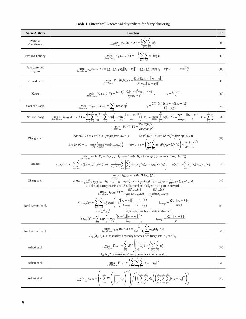
index with fifteen popular cluster validation indices in the literature. Table 1 lists these cluster validity indices. In this table, 𝑥𝑗

is the 𝑗𝑡ℎ data point, 𝑐 is the number of clusters, 𝑣𝑖 are cluster centers, 𝑢𝑖𝑗 is the degree of belonging of the 𝑗𝑡ℎ data to the

𝑖𝑡ℎcluster and 𝑁 is the total number of patterns in a given data set. The last three indices in this table are based on general type

2 fuzzy logic. Higher-order fuzzy clustering algorithms are very well suited to deal with the high levels of uncertainties present

in the majority of real-world applications. However, the immense computational complexity associated with such clustering

algorithms has been a great obstacle for the practical applications [16].

Now, we focus our attention on a well-known index from the second category which is the partition coefficient and exponential

separation index (PCAES) proposed by Wu and Yang [21]. VPCAES only utilizes membership values to validate the compactness

measure and does not consider the structure of data, i.e., the relative distance between objects and cluster centers [9]. For this

reason, it practiced weak in compactness measure. In order to tackle this problem, we use the fuzzy-possibilistic covariance

matrix and membership values in the proposed compactness measure. In this way, we involve characteristics like density,

shape, and patterns in the proposed index.

Additionally, VPCAES takes advantage of the exponential function to validate the separation measure, and also it involves the

distance between the mean of cluster centers and cluster centers. The stimulus behind taking the exponential function is that an

exponential operation is extremely effective in coping with Shannon entropy [27, 28] and Wu and Yang had asserted that an

exponential-type distance gives a robust property. Nevertheless, the experimental results demonstrate that this index gives

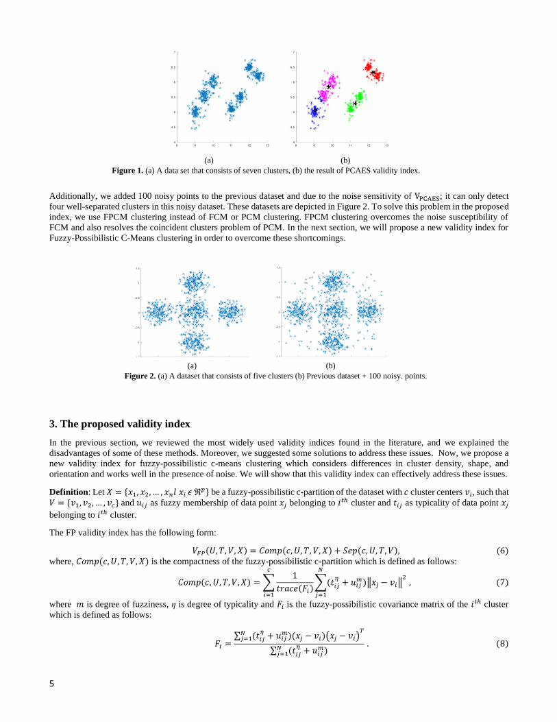
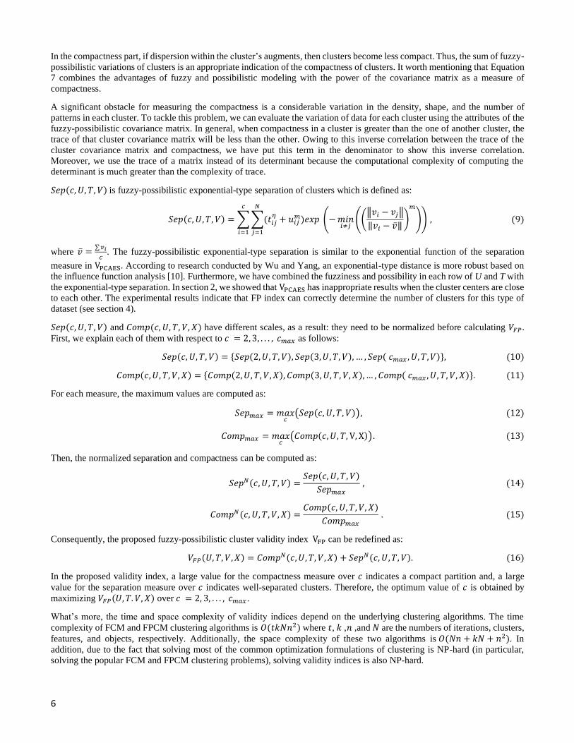
inappropriate results when the cluster centers are close to each other [9]. Figure 1 illustrates an example of the limited way in

which VPCAES loses its capability to indicate the appropriate number of clusters. Intuitively, we know that there are 7 fuzzy

clusters in this dataset. In Section 4, it will be demonstrated that VPCAES will detect four clusters. This problem occurs because

VPCAES calculates the separation between clusters using only centroid distances. To tackle these problems in the proposed

index, we use membership values and centroid distances to improve the separation measure.

What's more, a substantial feature of a validity index is its capability to handle noise and outliers. Because of the noise

sensitivity of FCM, and the structure of compactness measure in VPCAES; it is very susceptible to noises. To demonstrate the

noise sensitivity of PCAES validity index, we considered a 5-clusters dataset and the optimum number of clusters obtained

using VPCAES was 5.

4

Table 1. Fifteen well-known validity indices for fuzzy clustering.

Name/Authors Function Ref.

Partition

Coefficient 𝑚𝑎𝑥

2≤𝑐≤𝐶𝑚𝑎𝑥𝑉𝑃𝐶 (𝑈, 𝑉, 𝑋) =

1

𝑛∑∑𝑢𝑖𝑗

2

𝑁

𝑗=1

𝑐

𝑖=1

[15]

Partition Entropy 𝑚𝑖𝑛2≤𝑐≤𝐶𝑚𝑎𝑥

𝑉𝑃𝐸 (𝑈, 𝑉, 𝑋) = −1

𝑛∑∑𝑢𝑖𝑗

𝑁

𝑗=1

𝑐

𝑖=1

𝑙𝑜𝑔 𝑢𝑖𝑗 [15]

Fukuyama and

Sugeno 𝑚𝑖𝑛

2≤𝑐≤𝐶𝑚𝑎𝑥𝑉𝐹𝑆 (𝑈, 𝑉, 𝑋) = ∑ ∑ 𝑢𝑖𝑗

𝑚‖𝑥𝑗 − 𝑣𝑖‖2𝑁

𝑗=1𝑐𝑖=1 − ∑ ∑ 𝑢𝑖𝑗

𝑚‖𝑣𝑖 − �̅�‖2𝑁

𝑗=1𝑐𝑖=1 , �̅� =

∑𝑣𝑖

𝑐 [17]

Xie and Beni 𝑚𝑖𝑛2≤𝑐≤𝐶𝑚𝑎𝑥

𝑉𝑋𝐵 (𝑈, 𝑉, 𝑋) =∑ ∑ 𝑢𝑖𝑗

𝑚‖𝑥𝑗 − 𝑣𝑖‖2𝑁

𝑗=1𝑐𝑖=1

𝑁.𝑚𝑖𝑛𝑖,𝑗‖𝑣𝑖 − 𝑣𝑗‖

2 [18]

Kwon 𝑚𝑖𝑛2≤𝑐≤𝐶𝑚𝑎𝑥

𝑉𝐾 (𝑈, 𝑉, 𝑋) =∑ ∑ 𝑢𝑖𝑗

2 ‖𝑥𝑗−𝑣𝑖‖2

𝑁𝑗=1

𝑐𝑖=1 +

1𝑐∑ ‖𝑣𝑖−�̅�‖

2𝑐𝑖=1

𝑚𝑖𝑛𝑖≠𝑘

‖𝑣𝑖−𝑣𝑘‖2 , �̅� =

∑ 𝑥𝑗𝑁𝑗=1

𝑁 [19]

Gath and Geva 𝑚𝑖𝑛2≤𝑐≤𝐶𝑚𝑎𝑥

𝑉𝐹𝐻𝑉 (𝑈, 𝑉, 𝑋) =∑[𝑑𝑒𝑡(𝐹𝑖)]12

𝑐

𝑖=1

𝐹𝑖 =∑ (𝑢𝑖𝑗

𝑚)(𝑥𝑗 − 𝑣𝑖)(𝑥𝑗 − 𝑣𝑖)𝑇𝑁

𝑗=1

∑ (𝑢𝑖𝑗𝑚)𝑁

𝑗=1

[20]

Wu and Yang 𝑚𝑎𝑥2≤𝑐≤𝐶𝑚𝑎𝑥

𝑉𝑃𝐶𝐴𝐸𝑆 (𝑈, 𝑉, 𝑋) =∑∑𝑢𝑖𝑗

2

𝑢𝑀

𝑁

𝑗=1

𝑐

𝑖=1

−∑𝑒𝑥𝑝 (−min {𝑖≠𝑘

‖𝑣𝑖 − 𝑣𝑘‖2

𝐵𝑇})

𝑐

𝑖=1

, 𝑢𝑀 = 𝑚𝑖𝑛1≤𝑖≤𝑐

(∑𝑢𝑖𝑗𝑚)

𝑁

𝑗=1

, 𝐵𝑇 =∑‖𝑣𝑠 − �̅�‖

2

𝑐

𝑐

𝑠=1 , �̅� =∑

𝑥𝑗

𝑁

𝑁

𝑗=1

. [21]

Zhang et al.

𝑚𝑖𝑛2≤𝑐≤𝐶𝑚𝑎𝑥

𝑉𝑊 (𝑈, 𝑉) =𝑉𝑎𝑟𝑁(𝑈, 𝑉)

𝑆𝑒𝑝𝑁(𝑐, 𝑈)

𝑉𝑎𝑟𝑁(𝑈, 𝑉) = 𝑉𝑎𝑟 (𝑈, 𝑉) 𝑚𝑎𝑥𝑐(𝑉𝑎𝑟 (𝑈, 𝑉))⁄ 𝑆𝑒𝑝𝑁(𝑈, 𝑉) = 𝑆𝑒𝑝 (𝑐, 𝑈) 𝑚𝑎𝑥

𝑐(𝑆𝑒𝑝 (𝑐, 𝑈))⁄

𝑆𝑒𝑝 (𝑐, 𝑈) = 1 −𝑚𝑎𝑥𝑖≠𝑗

(𝑚𝑎𝑥𝑥𝑘∈𝑋

𝑚𝑖𝑛 (𝑢𝑖𝑘 , 𝑢𝑗𝑘)) 𝑉𝑎𝑟

(𝑈, 𝑉) = (∑∑𝑢𝑖𝑗

𝑁

𝑗=1

𝑐

𝑖=1

𝑑2(𝑥𝑗, 𝑣𝑖) 𝑛(𝑖)⁄ ) × (𝑐 + 1

𝑐 − 1)

12⁄

[22]

Rezaee

𝑚𝑖𝑛2≤𝑐≤𝐶𝑚𝑎𝑥

𝑉𝑆𝐶 (𝑐, 𝑈) = 𝑆𝑒𝑝 (𝑐, 𝑈) 𝑚𝑎𝑥𝑐(𝑆𝑒𝑝 (𝑐, 𝑈))⁄ + 𝐶𝑜𝑚𝑝 (𝑐, 𝑈) 𝑚𝑎𝑥

𝑐(𝐶𝑜𝑚𝑝 (𝑐, 𝑈))⁄

𝐶𝑜𝑚𝑝 (𝑐,𝑈) =∑∑𝑢𝑖𝑗2 ‖𝑥𝑗 − 𝑣𝑖‖

2𝑁

𝑗=1

𝑐

𝑖=1

, 𝑆𝑒𝑝 (𝑐, 𝑈) =2

𝑐(𝑐 − 1)∑ [∑(𝑚𝑖𝑛 (𝑢𝐹𝑝(𝑥𝑗),

𝑁

𝑗=1

𝑢𝐹𝑞(𝑥𝑗)))× ℎ(𝑥𝑗)]

𝑐

𝑝≠𝑞

, ℎ(𝑥𝑗) = −∑𝑢𝐹𝑝(𝑥𝑗) 𝑙𝑜𝑔𝑎 𝑢𝐹𝑞(𝑥𝑗)

𝑐

𝑖=1

[23]

Zhang et al.

𝑚𝑎𝑥2≤𝑐≤𝐶𝑚𝑎𝑥

𝑉𝑊𝐺𝐿𝐼 = (2𝑀𝑀𝐷+ 𝑄𝐵) 3⁄ ,

𝑀𝑀𝐷 =1

𝑛∑ 𝑚𝑎𝑥

1≤𝑖≤𝐶𝑢𝑖𝑗 𝑁

𝑗=1 , 𝑄𝐵 = ∑ (𝑒𝑖𝑗 − 𝑎𝑖𝑎𝑗)𝑖 , 𝑗 = 𝑚𝑎𝑥𝑘(𝑒𝑖𝑘) , 𝑎𝑖 = ∑ 𝑒𝑖𝑗𝑖 =

1

2𝑀∑ ∑ 𝐴(𝑖, 𝑗)𝑗∈𝑉 𝑖∈𝑉𝑙

𝐴 is the adjacency matrix and M is the number of edges in a bipartite network.

[24]

Fazel Zarandi et al.

𝑚𝑎𝑥2≤𝑐≤𝐶𝑚𝑎𝑥

𝑉𝐸𝐶𝐴𝑆 (𝑐) =𝐸𝐶𝑐𝑜𝑚𝑝(𝑐)

𝑚𝑎𝑥𝑐(𝐸𝐶𝑐𝑜𝑚𝑝(𝑐))

−𝐸𝑆𝑠𝑒𝑝(𝑐)

𝑚𝑎𝑥𝑐(𝐸𝑆𝑠𝑒𝑝(𝑐))

𝐸𝐶𝑐𝑜𝑚𝑝(𝑐) =∑∑𝑢𝑖𝑗𝑚

𝑁

𝑗=1

𝑐

𝑖=1

𝑒𝑥𝑝(−(‖𝑥𝑗 − 𝑣𝑖‖

2

𝛽𝑐𝑜𝑚𝑝+

1

𝑐 + 1)) 𝛽𝑐𝑜𝑚𝑝 =

∑ ‖𝑥𝑘 − �̅�‖2𝑁

𝑘=1

𝑛(𝑖)

�̅� = ∑𝑥𝑗

𝑁

𝑁𝑗=1 𝑛(𝑖) is the number of data in cluster i

𝐸𝑆𝑠𝑒𝑝(𝑐) =∑𝑒𝑥𝑝(−𝑚𝑖𝑛𝑖≠𝑗

{(𝑐 − 1)‖𝑣𝑖 − 𝑣𝑗‖

2

𝛽𝑠𝑒𝑝})

𝑐

𝑖=1

𝛽𝑐𝑜𝑚𝑝 =∑ ‖𝑣𝑏 − �̅�‖

2𝑐𝑏=1

𝑐

[9]

Fazel Zarandi et al. 𝑚𝑖𝑛

2≤𝑐≤𝐶𝑚𝑎𝑥𝑉𝐹𝑁𝑇 (𝑈, 𝑉, 𝑋) =

2

𝑐(𝑐 − 1)∑𝑆𝑟𝑒𝑙(𝐴𝑝, 𝐴𝑞)

𝑐

𝑝≠𝑞

𝑆𝑟𝑒𝑙(𝐴𝑝, 𝐴𝑞) is the relative similarity between two fuzzy sets 𝐴𝑝 and 𝐴𝑞.

[25]

Askari et al. 𝑚𝑖𝑛

2≤𝑐≤𝐶𝑚𝑎𝑥𝑉𝐺𝑃𝐹1 =∑𝑅𝑖

𝑟(√∏𝜆𝑞𝑖

𝑟

𝑞=1

)−1𝑐

𝑖=1

∑∑𝑢𝑖𝑗𝑚

𝑁

𝑗=1

𝑐

𝑖=1

⁄

𝜆𝑞𝑖 is 𝑞𝑡ℎ eigenvalue of fuzzy covariance norm matrix

[26]

Askari et al. 𝑚𝑎𝑥2≤𝑐≤𝐶𝑚𝑎𝑥

𝑉𝐺𝑃𝐹2 =1

𝑐∑∑∑|𝑢𝑘𝑗

− 𝑢𝑖𝑗 |𝑚

𝑁

𝑗=1

𝑐

𝑖=1

𝑐

𝑘=1

[26]

Askari et al. 𝑚𝑖𝑛2≤𝑐≤𝐶𝑚𝑎𝑥

𝑉𝐺𝑃𝐹3 =

(

𝑐∑𝑅𝑖

𝑟(√∏𝜆𝑞𝑖

𝑟

𝑞=1

)

−1

𝑐

𝑖=1

)

((∑∑𝑢𝑖𝑗𝑚

𝑁

𝑗=1

𝑐

𝑖=1

)(∑∑∑|𝑢𝑘𝑗 − 𝑢𝑖𝑗

|𝑚

𝑁

𝑗=1

𝑐

𝑖=1

𝑐

𝑘=1

))⁄ [26]

5

Additionally, we added 100 noisy points to the previous dataset and due to the noise sensitivity of VPCAES; it can only detect

four well-separated clusters in this noisy dataset. These datasets are depicted in Figure 2. To solve this problem in the proposed

index, we use FPCM clustering instead of FCM or PCM clustering. FPCM clustering overcomes the noise susceptibility of

FCM and also resolves the coincident clusters problem of PCM. In the next section, we will propose a new validity index for

Fuzzy-Possibilistic C-Means clustering in order to overcome these shortcomings.

3. The proposed validity index

In the previous section, we reviewed the most widely used validity indices found in the literature, and we explained the

disadvantages of some of these methods. Moreover, we suggested some solutions to address these issues. Now, we propose a

new validity index for fuzzy-possibilistic c-means clustering which considers differences in cluster density, shape, and

orientation and works well in the presence of noise. We will show that this validity index can effectively address these issues.

Definition: Let 𝑋 = {𝑥1, 𝑥2, … , 𝑥𝑛𝑙 𝑥𝑖 𝜖 ℜ𝑝} be a fuzzy-possibilistic c-partition of the dataset with 𝑐 cluster centers 𝑣𝑖, such that

𝑉 = {𝑣1, 𝑣2, … , 𝑣𝑐} and 𝑢𝑖𝑗 as fuzzy membership of data point 𝑥𝑗 belonging to 𝑖𝑡ℎ cluster and 𝑡𝑖𝑗 as typicality of data point 𝑥𝑗

belonging to 𝑖𝑡ℎ cluster.

The FP validity index has the following form:

𝑉𝐹𝑃(𝑈,𝑇, 𝑉, 𝑋) = 𝐶𝑜𝑚𝑝(𝑐, 𝑈, 𝑇, 𝑉, 𝑋) + 𝑆𝑒𝑝(𝑐, 𝑈, 𝑇, 𝑉), (6) where, 𝐶𝑜𝑚𝑝(𝑐, 𝑈, 𝑇, 𝑉, 𝑋) is the compactness of the fuzzy-possibilistic c-partition which is defined as follows:

𝐶𝑜𝑚𝑝(𝑐, 𝑈, 𝑇, 𝑉,𝑋) =∑1

𝑡𝑟𝑎𝑐𝑒(𝐹𝑖)

𝑐

𝑖=1

∑(𝑡𝑖𝑗𝜂+ 𝑢𝑖𝑗

𝑚)‖𝑥𝑗 − 𝑣𝑖‖2

𝑁

𝑗=1

, (7)

where 𝑚 is degree of fuzziness, η is degree of typicality and 𝐹𝑖 is the fuzzy-possibilistic covariance matrix of the 𝑖𝑡ℎ cluster

which is defined as follows:

𝐹𝑖 =∑ (𝑡𝑖𝑗

𝜂+ 𝑢𝑖𝑗

𝑚)(𝑥𝑗 − 𝑣𝑖)(𝑥𝑗 − 𝑣𝑖)𝑇𝑁

𝑗=1

∑ (𝑡𝑖𝑗𝜂+ 𝑢𝑖𝑗

𝑚)𝑁𝑗=1

. (8)

(a) (b)

Figure 1. (a) A data set that consists of seven clusters, (b) the result of PCAES validity index.

(a) (b)

Figure 2. (a) A dataset that consists of five clusters (b) Previous dataset + 100 noisy. points.

6

In the compactness part, if dispersion within the cluster’s augments, then clusters become less compact. Thus, the sum of fuzzy-

possibilistic variations of clusters is an appropriate indication of the compactness of clusters. It worth mentioning that Equation

7 combines the advantages of fuzzy and possibilistic modeling with the power of the covariance matrix as a measure of

compactness.

A significant obstacle for measuring the compactness is a considerable variation in the density, shape, and the number of

patterns in each cluster. To tackle this problem, we can evaluate the variation of data for each cluster using the attributes of the

fuzzy-possibilistic covariance matrix. In general, when compactness in a cluster is greater than the one of another cluster, the

trace of that cluster covariance matrix will be less than the other. Owing to this inverse correlation between the trace of the

cluster covariance matrix and compactness, we have put this term in the denominator to show this inverse correlation.

Moreover, we use the trace of a matrix instead of its determinant because the computational complexity of computing the

determinant is much greater than the complexity of trace.

𝑆𝑒𝑝(𝑐, 𝑈, 𝑇, 𝑉) is fuzzy-possibilistic exponential-type separation of clusters which is defined as:

𝑆𝑒𝑝(𝑐, 𝑈, 𝑇, 𝑉) =∑∑(𝑡𝑖𝑗𝜂+ 𝑢𝑖𝑗

𝑚)𝑒𝑥𝑝 (−𝑚𝑖𝑛𝑖≠𝑗

((‖𝑣𝑖 − 𝑣𝑗‖

‖𝑣𝑖 − �̅�‖)

𝑚

))

𝑁

𝑗=1

𝑐

𝑖=1

, (9)

where �̅� =∑𝑣𝑖

𝑐. The fuzzy-possibilistic exponential-type separation is similar to the exponential function of the separation

measure in VPCAES. According to research conducted by Wu and Yang, an exponential-type distance is more robust based on

the influence function analysis [10]. Furthermore, we have combined the fuzziness and possibility in each row of U and T with

the exponential-type separation. In section 2, we showed that VPCAES has inappropriate results when the cluster centers are close

to each other. The experimental results indicate that FP index can correctly determine the number of clusters for this type of

dataset (see section 4).

𝑆𝑒𝑝(𝑐, 𝑈, 𝑇, 𝑉) and 𝐶𝑜𝑚𝑝(𝑐, 𝑈, 𝑇, 𝑉, 𝑋) have different scales, as a result: they need to be normalized before calculating 𝑉𝐹𝑃.

First, we explain each of them with respect to 𝑐 = 2, 3, . . . , 𝑐𝑚𝑎𝑥 as follows:

𝑆𝑒𝑝(𝑐, 𝑈, 𝑇, 𝑉) = {𝑆𝑒𝑝(2,𝑈, 𝑇, 𝑉), 𝑆𝑒𝑝(3,𝑈, 𝑇, 𝑉), … , 𝑆𝑒𝑝( 𝑐𝑚𝑎𝑥 , 𝑈, 𝑇, 𝑉)}, (10)

𝐶𝑜𝑚𝑝(𝑐,𝑈, 𝑇, 𝑉, 𝑋) = {𝐶𝑜𝑚𝑝(2,𝑈, 𝑇, 𝑉,𝑋), 𝐶𝑜𝑚𝑝(3, 𝑈, 𝑇, 𝑉, 𝑋),… , 𝐶𝑜𝑚𝑝( 𝑐𝑚𝑎𝑥 , 𝑈, 𝑇, 𝑉, 𝑋)}. (11)

For each measure, the maximum values are computed as:

𝑆𝑒𝑝𝑚𝑎𝑥 = 𝑚𝑎𝑥𝑐(𝑆𝑒𝑝(𝑐, 𝑈, 𝑇, 𝑉)), (12)

𝐶𝑜𝑚𝑝𝑚𝑎𝑥 = 𝑚𝑎𝑥𝑐(𝐶𝑜𝑚𝑝(𝑐,𝑈, 𝑇, V, X)). (13)

Then, the normalized separation and compactness can be computed as:

𝑆𝑒𝑝𝑁(𝑐,𝑈, 𝑇, 𝑉) =𝑆𝑒𝑝(𝑐, 𝑈, 𝑇, 𝑉)

𝑆𝑒𝑝𝑚𝑎𝑥 , (14)

𝐶𝑜𝑚𝑝𝑁(𝑐, 𝑈, 𝑇, 𝑉, 𝑋) =𝐶𝑜𝑚𝑝(𝑐, 𝑈, 𝑇, 𝑉, 𝑋)

𝐶𝑜𝑚𝑝𝑚𝑎𝑥 . (15)

Consequently, the proposed fuzzy-possibilistic cluster validity index VFP can be redefined as:

𝑉𝐹𝑃(𝑈, 𝑇, 𝑉,𝑋) = 𝐶𝑜𝑚𝑝𝑁(𝑐,𝑈, 𝑇, 𝑉,𝑋) + 𝑆𝑒𝑝𝑁(𝑐, 𝑈, 𝑇, 𝑉). (16)

In the proposed validity index, a large value for the compactness measure over 𝑐 indicates a compact partition and, a large

value for the separation measure over 𝑐 indicates well-separated clusters. Therefore, the optimum value of 𝑐 is obtained by

maximizing 𝑉𝐹𝑃(𝑈, 𝑇. 𝑉, 𝑋) over 𝑐 = 2, 3, . . . , 𝑐𝑚𝑎𝑥 .

What’s more, the time and space complexity of validity indices depend on the underlying clustering algorithms. The time

complexity of FCM and FPCM clustering algorithms is 𝑂(𝑡𝑘𝑁𝑛2) where 𝑡, 𝑘 ,𝑛 ,and 𝑁 are the numbers of iterations, clusters,

features, and objects, respectively. Additionally, the space complexity of these two algorithms is 𝑂(𝑁𝑛 + 𝑘𝑁 + 𝑛2). In

addition, due to the fact that solving most of the common optimization formulations of clustering is NP-hard (in particular,

solving the popular FCM and FPCM clustering problems), solving validity indices is also NP-hard.

7

4. A procedure for determining the parameters of the proposed method

In addition to the number of clusters, FPCM and its various extensions require a priori selection of the degree of fuzziness (m)

and the degree of typicality (η). During the past few decades, various ranges and values for the optimum degree of fuzziness

have been proposed. Here, we briefly review studies that have proposed a range or a method for determining the optimal degree

of fuzziness. Then, we will present an efficient procedure for determining an optimal value for 𝑚 and 𝜂. Bezdek was one of

the first scientists who introduced a heuristic procedure for finding an optimum value for 𝑚 [29]. McBratney and Moore [30]

observed that the objective function value 𝐽𝑚 reduces monotonically with augmenting 𝑐 and 𝑚. Furthermore, they demonstrated

that the greatest change in 𝐽𝑚, occurred around 𝑚 = 2. Choe and Jordan [31] proposed an algorithm for finding the optimum

𝑚 using the concept of fuzzy decision theory. Yu et al. [32] defined two theoretical rules for selecting the weighting exponent

in the FCM. According to their approach, they revealed the relationship between the stability of the fixed points of the FCM

and the data set itself. Okeke and Karnieli [33] presented a procedure using the output of the fuzzy clustering. Their method

predicts the original data using the idea of linear mixture modeling. The formula for reconstructing the original dataset has the

following form:

�̃� = �̃�𝑈, (17)

where, �̃� is vector of predicted dataset. �̃� is vector of the FCM output centers and 𝑈 is the matrix of membership functions.

Next, the differences between the predicted dataset and the original dataset are specified by the following formula [33]:

𝜎 = ‖𝑋 − �̃�‖, 𝜎 > 0, ∀𝑚 (18)

Eventually, the degree of fuzziness which corresponds to the minimum of 𝜎 is the optimum value [33].

Since the amounts of 𝜂 and m play an important role in FP index, we present an algorithm to tackle this problem. In the proposed

algorithm, FPCM clustering is run for different values of 𝑚, 𝜂 and 𝑐. After that, the original dataset is reconstructed from the

outputs of FPCM algorithm using the following formulas:

�̃�𝑈 = �̃�𝑈 , (19)

�̃�𝑇 = �̃��̃�𝑁 , (20)

where, �̃�𝑈is the vector of the predicted dataset using membership functions matrix. 𝑈 is the matrix of membership functions

for the FPCM algorithm and �̃� is the vector of the FPCM centers. �̃�𝑇is the vector of the predicted dataset using normalized

typicality matrix. �̃�𝑁 represents the normalized typicality matrix and is defined as:

�̃�𝑁(𝑐, 𝑁) =�̃�(𝑐, 𝑁)

∑ �̃�(𝑐, 𝑁)𝑐

. (21)

Then, the difference between the predicted dataset and the original dataset is determined by the root mean squared error

(RMSE).

𝑅𝑀𝑆𝐸 = √∑ ∑ (𝑥𝑖𝑑 − �̃�𝑖𝑑)

2𝑐𝑖=1

𝑁𝑑=1

𝑁 , (22)

where, 𝑥𝑖𝑑 and �̃�𝑖𝑑 are the actual and predicted datasets, respectively, 𝑑 is the number of data and 𝑐 is the number of clusters.

Thus, 𝑅𝑀𝑆𝐸𝑇𝑜𝑡𝑎𝑙 can be defined as:

𝑅𝑀𝑆𝐸𝑇𝑜𝑡𝑎𝑙 = 𝑅𝑀𝑆𝐸𝑇+𝑅𝑀𝑆𝐸𝑈 , (23)

where, 𝑅𝑀𝑆𝐸𝑇 and 𝑅𝑀𝑆𝐸𝑈 are the root mean squared errors computed by �̃�𝑇and �̃�𝑈, respectively. After that, cumulative

root mean square error (CRMSE) for every pair of (𝑚, 𝜂) is defined as:

𝐶𝑅𝑀𝑆𝐸 (𝑚, 𝜂) = ∑ 𝑅𝑀𝑆𝐸𝑇𝑜𝑡𝑎𝑙(𝑚, 𝜂, 𝑐)𝑐𝑚𝑎𝑥𝑐=2 , (24)

where, 𝑐𝑚𝑎𝑥 is the maximum number of clusters. Finally, an optimal value for m and η can be found by minimizing 𝐶𝑅𝑀𝑆𝐸 over

𝜂 and m. The steps of the proposed algorithm can be seen in Algorithm 1.

Algorithm 1 runs FPCM clustering and computes 𝑉𝐹𝑃 with respect to 𝑐 = 2, 3, . . . , 𝑐𝑚𝑎𝑥 . There is no universal agreement on

what value to use for cmax. The value of 𝑐𝑚𝑎𝑥 can be selected in accordance with the user’s knowledge about the dataset;

however, as this is not always feasible, a lot of researchers use cmax = √N [34]. What's more, the variation of FP index values

for all experimental data sets demonstrates that the maximum of VFP exists between 2 and √𝑁 (see Section 4). In order to show

the behavior of Algorithm 1, the dataset which is shown in Fig 2 (b) is used as input data. Let 𝑐𝑚𝑎𝑥 = 8 ,𝑚𝑚𝑎𝑥 = 5 and 𝜂𝑚𝑎𝑥 =

8

5 be the initial values for Algorithm 1(the theoretical rules proposed by Yu et al. are used in order to define 𝑚𝑚𝑎𝑥 and 𝜂𝑚𝑎𝑥).

Table 2 shows the cumulative root mean square error of this dataset. The elements of this table are the degree of typicality (𝜂)

and the degree of fuzziness (𝑚) as input variables and CRMSE as results.

For instance, for 𝑚 = 1.2, 𝜂 = 2.2, CRMSE is 6.316. According to Table 2, the suitable values of 𝑚 and 𝜂 can be found by

𝐶𝑅𝑀𝑆𝐸 (𝑚∗, 𝜂∗) = 𝑚𝑖𝑛𝜂𝑚𝑖𝑛𝑚(𝐶𝑅𝑀𝑆𝐸). Therefore, the suitable values of m and η are 1.6 and 2.2, respectively. Finally, the

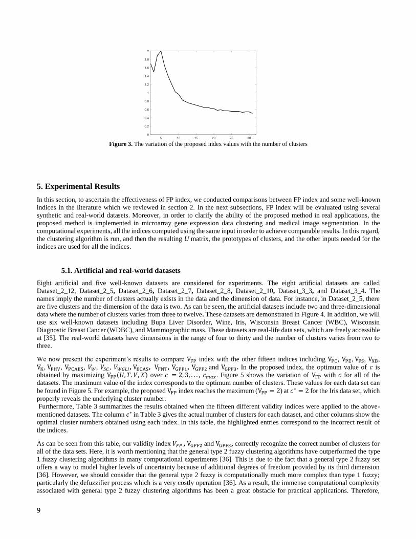
optimal number of clusters obtained using Algorithm 1 is five with 𝑚 = 1.6 and 𝜂 = 2.2. Figure 3 shows the variation of the

proposed index values with the number of clusters for this dataset.

Algorithm 1: The proposed algorithm for determining the suitable values of c, m and η

➢ Define the initial parameters:

• Set c=2 and determine the maximum number of the clusters (𝑐𝑚𝑎𝑥)

• Set m=1.1 and determine the maximum value for the degree of fuzziness (𝑚𝑚𝑎𝑥)

• Set 𝜂 =1.1 and determine the maximum value for the degree of typicality (𝜂𝑚𝑎𝑥)

For 𝑐 = 2 to 𝑐𝑚𝑎𝑥

For 𝑚 = 1.1 to 𝑚𝑚𝑎𝑥

For 𝜂 = 1.1 to η𝑚𝑎𝑥

Compute fuzzy prototypes �̃� , membership functions (�̃�) and typicality (�̃�) using FPCM algorithm.

Reconstruct the original dataset using Equation 19 and Equation 20.

Compute 𝑅𝑀𝑆𝐸𝑇𝑜𝑡𝑎𝑙 , the difference between the original dataset and the predicted dataset using Equation 23.

End for

End for

End for

Compute 𝐶𝑅𝑀𝑆𝐸 for every pair of (𝑚, 𝜂) using Equation 24.

Find 𝑚∗ and 𝜂∗ such that 𝐶𝑅𝑀𝑆𝐸 (𝑚∗, 𝜂∗) = min𝜂min𝑚(𝐶𝑅𝑀𝑆𝐸).

Compute the FP index (VFP) with 𝑚 = 𝑚∗ and 𝜂 = 𝜂∗ for 𝑐 = 2, 3, . . . , cmax

Determine the optimum value of 𝑐 by maximizing VFP over 𝑐 = 2, 3, . . . , cmax.

Table 2. CRMSE values for different η and m.

1.2 1.6 2 2.2 2.6 3 3.4 3.8 4.2 4.4 4.6 5 m

η

1.2 6.225 6.344 6.285 6.319 6.302 6.265 6.357 6.316 6.228 6.329 6.278 6.367

1.6 6.333 6.328 6.383 6.408 6.343 6.305 6.333 6.287 6.238 6.321 6.278 6.390

2 6.350 6.343 6.281 6.340 6.307 6.314 6.310 6.351 6.336 6.357 6.363 6.294

2.2 6.316 6.190 6.338 6.252 6.381 6.405 6.597 6.342 6.322 6.316 6.281 6.421

2.6 6.313 6.307 6.346 6.440 6.341 6.331 6.239 6.244 6.254 6.338 6.330 6.313

3 6.312 6.292 6.305 6.311 6.355 6.265 6.282 6.313 6.318 6.360 6.221 6.327

3.4 6.249 6.278 6.325 6.342 6.305 6.303 6.244 6.301 6.289 6.297 6.382 6.309

3.8 6.278 6.293 6.542 6.252 6.337 6.350 6.305 6.318 6.289 6.210 6.290 6.321

4.2 6.363 6.365 6.306 6.315 6.406 6.323 6.354 6.330 6.327 6.365 6.273 6.269

4.4 6.308 6.302 6.658 6.289 6.339 6.338 6.328 6.288 6.306 6.649 6.339 6.288

4.6 6.265 6.328 6.367 6.337 6.275 6.313 6.338 6.456 6.349 6.335 6.316 6.281

5 6.287 6.263 6.313 6.298 6.322 6.292 6.354 6.347 6.358 6.292 6.277 6.421

9

Figure 3. The variation of the proposed index values with the number of clusters

5. Experimental Results

In this section, to ascertain the effectiveness of FP index, we conducted comparisons between FP index and some well-known

indices in the literature which we reviewed in section 2. In the next subsections, FP index will be evaluated using several

synthetic and real-world datasets. Moreover, in order to clarify the ability of the proposed method in real applications, the

proposed method is implemented in microarray gene expression data clustering and medical image segmentation. In the

computational experiments, all the indices computed using the same input in order to achieve comparable results. In this regard,

the clustering algorithm is run, and then the resulting U matrix, the prototypes of clusters, and the other inputs needed for the

indices are used for all the indices.

5.1. Artificial and real-world datasets

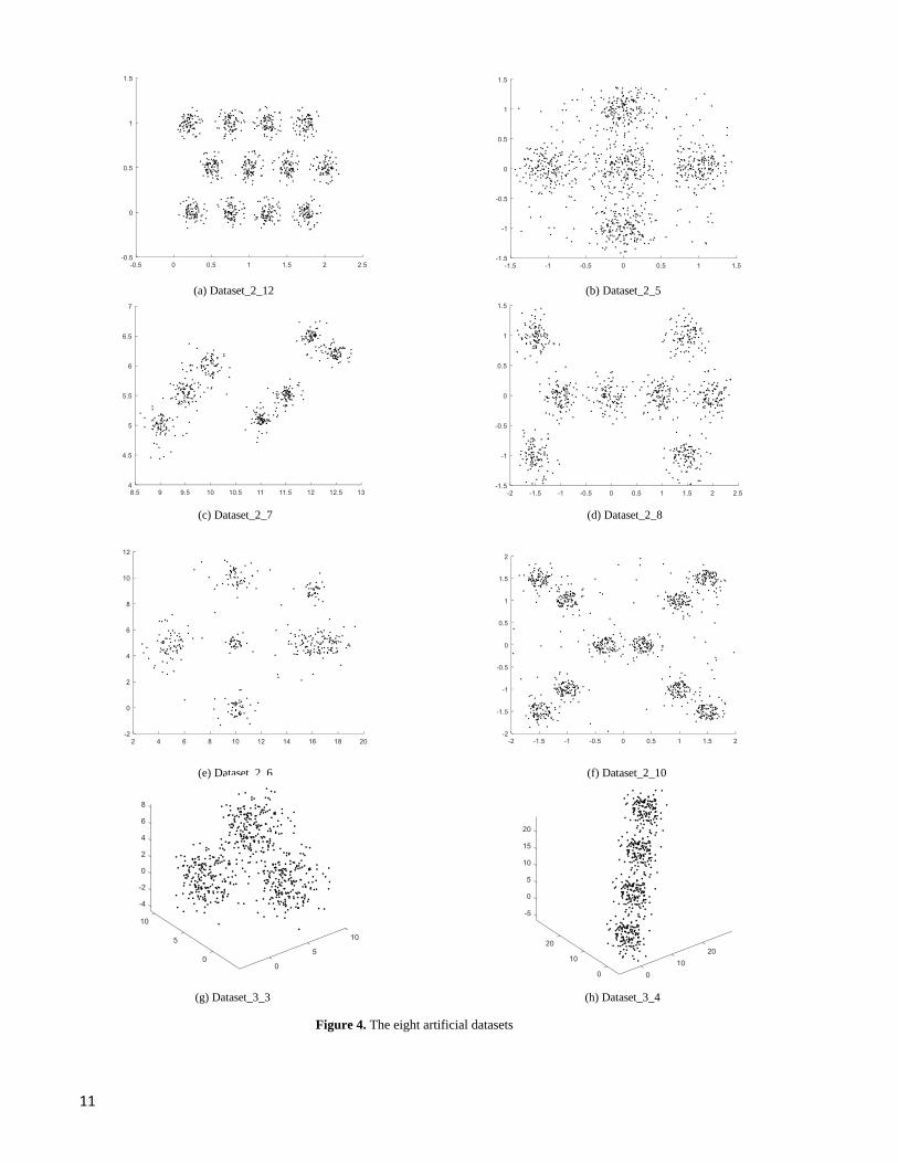
Eight artificial and five well-known datasets are considered for experiments. The eight artificial datasets are called

Dataset_2_12, Dataset_2_5, Dataset_2_6, Dataset_2_7, Dataset_2_8, Dataset_2_10, Dataset_3_3, and Dataset_3_4. The

names imply the number of clusters actually exists in the data and the dimension of data. For instance, in Dataset_2_5, there

are five clusters and the dimension of the data is two. As can be seen, the artificial datasets include two and three-dimensional

data where the number of clusters varies from three to twelve. These datasets are demonstrated in Figure 4. In addition, we will

use six well-known datasets including Bupa Liver Disorder, Wine, Iris, Wisconsin Breast Cancer (WBC), Wisconsin

Diagnostic Breast Cancer (WDBC), and Mammographic mass. These datasets are real-life data sets, which are freely accessible

at [35]. The real-world datasets have dimensions in the range of four to thirty and the number of clusters varies from two to

three.

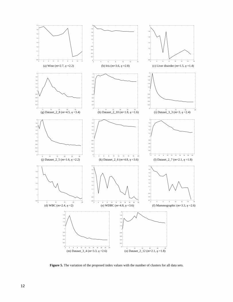
We now present the experiment’s results to compare VFP index with the other fifteen indices including VPC, VPE, VFS, VXB,

VK, VFHV, VPCAES, 𝑉𝑊, 𝑉𝑆𝐶 , 𝑉𝑊𝐺𝐿𝐼 , VECAS, VFNT, VGPF1, VGPF2 and VGPF3. In the proposed index, the optimum value of 𝑐 is

obtained by maximizing VFP(𝑈,𝑇. 𝑉, 𝑋) over 𝑐 = 2, 3, . . . , 𝑐𝑚𝑎𝑥. Figure 5 shows the variation of VFP with 𝑐 for all of the

datasets. The maximum value of the index corresponds to the optimum number of clusters. These values for each data set can

be found in Figure 5. For example, the proposed VFP index reaches the maximum (VFP = 2) at 𝑐∗ = 2 for the Iris data set, which

properly reveals the underlying cluster number.

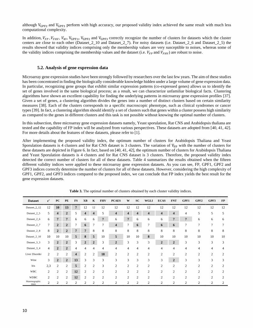
Furthermore, Table 3 summarizes the results obtained when the fifteen different validity indices were applied to the above-

mentioned datasets. The column 𝑐∗ in Table 3 gives the actual number of clusters for each dataset, and other columns show the

optimal cluster numbers obtained using each index. In this table, the highlighted entries correspond to the incorrect result of

the indices.

As can be seen from this table, our validity index 𝑉𝐹𝑃 , VGPF2 and VGPF3, correctly recognize the correct number of clusters for

all of the data sets. Here, it is worth mentioning that the general type 2 fuzzy clustering algorithms have outperformed the type

1 fuzzy clustering algorithms in many computational experiments [36]. This is due to the fact that a general type 2 fuzzy set

offers a way to model higher levels of uncertainty because of additional degrees of freedom provided by its third dimension

[36]. However, we should consider that the general type 2 fuzzy is computationally much more complex than type 1 fuzzy;

particularly the defuzzifier process which is a very costly operation [36]. As a result, the immense computational complexity

associated with general type 2 fuzzy clustering algorithms has been a great obstacle for practical applications. Therefore,

10

although VGPF2 and VGPF3 perform with high accuracy, our proposed validity index achieved the same result with much less

computational complexity.

In addition, 𝑉𝐹𝑃 , 𝑉𝐹𝐻𝑉, 𝑉𝑊, VGPF1, VGPF2 and VGPF3 correctly recognize the number of clusters for datasets which the cluster

centers are close to each other (Dataset_2_10 and Dataset_2_7). For noisy datasets (i.e. Dataset_2_6 and Dataset_2_5) the

results showed that validity indices comprising only the membership values are very susceptible to noises, whereas some of

the validity indices comprising the membership values and the dataset (i.e. 𝑉𝐹𝑃 and 𝑉𝐹𝐻𝑉) are robust to noise.

5.2. Analysis of gene expression data

Microarray gene expression studies have been strongly followed by researchers over the last few years. The aim of these studies

has been concentrated in finding the biologically considerable knowledge hidden under a large volume of gene expression data.

In particular, recognizing gene groups that exhibit similar expression patterns (co-expressed genes) allows us to identify the

set of genes involved in the same biological process; as a result, we can characterize unfamiliar biological facts. Clustering

algorithms have shown an excellent capability for finding the underlying patterns in microarray gene expression profiles [37].

Given a set of genes, a clustering algorithm divides the genes into a number of distinct clusters based on certain similarity

measures [38]. Each of the clusters corresponds to a specific macroscopic phenotype, such as clinical syndromes or cancer

types [39]. In fact, a clustering algorithm should identify a set of clusters such that genes within a cluster possess high similarity

as compared to the genes in different clusters and this task is not possible without knowing the optimal number of clusters.

In this subsection, three microarray gene expression datasets namely, Yeast sporulation, Rat CNS and Arabidopsis thaliana are

tested and the capability of FP index will be analyzed from various perspectives. These datasets are adopted from [40, 41, 42].

For more details about the features of these datasets, please refer to [1].

After implementing the proposed validity index, the optimum number of clusters for Arabidopsis Thaliana and Yeast

Sporulation datasets is 4 clusters and for Rat CNS dataset is 3 clusters. The variation of VFP with the number of clusters for

these datasets are depicted in Figure 6. In fact, based on [40, 41, 42], the optimum number of clusters for Arabidopsis Thaliana

and Yeast Sporulation datasets is 4 clusters and for Rat CNS dataset is 3 clusters. Therefore, the proposed validity index

detected the correct number of clusters for all of these datasets. Table 4 summarizes the results obtained when the fifteen

different validity indices were applied to these microarray gene expression datasets. As you can see, FP, GPF1, GPF2 and

GPF3 indices correctly determine the number of clusters for all of these datasets. However, considering the high complexity of

GPF1, GPF2, and GPF3 indices compared to the proposed index, we can conclude that FP index yields the best result for the

gene expression datasets.

Table 3. The optimal number of clusters obtained by each cluster validity indices.

Dataset 𝒄∗ PC PE FS XB K FHV PCAES W SC WGLI ECAS FNT GPF1 GPF2 GPF3 FP

Dataset_2_12 12 10 13 7 12 12 12 12 12 12 12 12 12 12 12 12 12

Dataset_2_5 5 4 2 5 4 4 5 4 4 4 4 4 4 4 5 5 5

Dataset_2_6 6 7 7 6 6 6 7 6 7 6 6 6 7 7 6 6 6

Dataset_2_7 7 2 2 7 6 7 7 4 7 6 7 6 6 7 7 7 7

Dataset_2_8 8 2 2 7 7 8 8 8 8 8 8 8 8 8 8 8 8

Dataset_2_10 10 10 10 5 8 5 10 5 10 10 8 10 10 10 10 10 10

Dataset_3_3 3 2 2 3 2 2 3 2 3 3 3 2 2 3 3 3 3

Dataset_3_4 4 2 2 4 4 4 4 4 4 4 4 4 4 4 4 4 4

Liver Disorder 2 2 2 4 2 2 18 2 2 2 2 2 2 2 2 2 2

Wine 3 2 2 13 3 3 3 3 3 3 3 3 2 3 3 3 3

Iris 2,3 2 2 5 2 2 3 2 2 2 2 2 2 2 2 2 2

WBC 2 2 2 12 2 2 2 2 2 2 2 2 2 2 2 2 2

WDBC 2 2 2 12 2 2 2 2 2 2 2 2 2 2 2 2 2 Mammographic

mass 2 2 2 2 2 2 2 2 2 2 2 2 2 2 2 2 2

11

(a) Dataset_2_12 (b) Dataset_2_5

(c) Dataset_2_7 (d) Dataset_2_8

(e) Dataset_2_6 (f) Dataset_2_10

(g) Dataset_3_3 (h) Dataset_3_4

Figure 4. The eight artificial datasets

12

Figure 5. The variation of the proposed index values with the number of clusters for all data sets.

(d) WBC (m=2.4, η =2) (e) WDBC (m=4.8, η =3.6) (f) Mammographic (m=3.3, η =2.6)

(m) Dataset_3_4 (m=3.3, η =2.6) (n) Dataset_2_12 (m=2.1, η =1.8)

(j) Dataset_2_5 (m=1.6, η =2.2) (k) Dataset_2_6 (m=4.8, η =3.6) (l) Dataset_2_7 (m=2.1, η =1.8)

(g) Dataset_2_8 (m=4.5, η =3.4) (h) Dataset_2_10 (m=1.8, η =1.6) (i) Dataset_3_3 (m=3, η =2.4)

(a) Wine (m=2.7, η =2.2) (b) Iris (m=3.6, η =2.8) (c) Liver disorder (m=1.5, η =1.4)

13

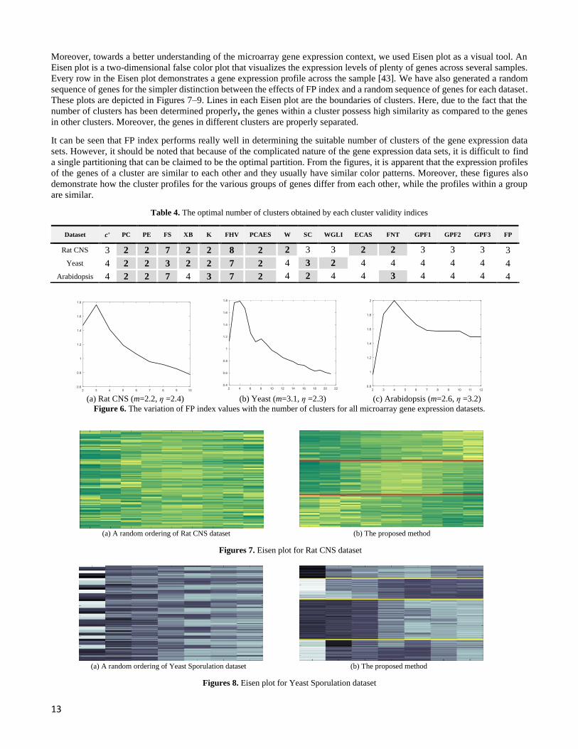
Moreover, towards a better understanding of the microarray gene expression context, we used Eisen plot as a visual tool. An

Eisen plot is a two-dimensional false color plot that visualizes the expression levels of plenty of genes across several samples.

Every row in the Eisen plot demonstrates a gene expression profile across the sample [43]. We have also generated a random

sequence of genes for the simpler distinction between the effects of FP index and a random sequence of genes for each dataset.

These plots are depicted in Figures 7–9. Lines in each Eisen plot are the boundaries of clusters. Here, due to the fact that the

number of clusters has been determined properly, the genes within a cluster possess high similarity as compared to the genes

in other clusters. Moreover, the genes in different clusters are properly separated.

It can be seen that FP index performs really well in determining the suitable number of clusters of the gene expression data

sets. However, it should be noted that because of the complicated nature of the gene expression data sets, it is difficult to find

a single partitioning that can be claimed to be the optimal partition. From the figures, it is apparent that the expression profiles

of the genes of a cluster are similar to each other and they usually have similar color patterns. Moreover, these figures also

demonstrate how the cluster profiles for the various groups of genes differ from each other, while the profiles within a group

are similar.

Table 4. The optimal number of clusters obtained by each cluster validity indices

(a) Rat CNS (m=2.2, η =2.4) (b) Yeast (m=3.1, η =2.3) (c) Arabidopsis (m=2.6, η =3.2)

Figure 6. The variation of FP index values with the number of clusters for all microarray gene expression datasets.

(a) A random ordering of Rat CNS dataset (b) The proposed method

Figures 7. Eisen plot for Rat CNS dataset

(a) A random ordering of Yeast Sporulation dataset (b) The proposed method

Figures 8. Eisen plot for Yeast Sporulation dataset

Dataset 𝒄∗ PC PE FS XB K FHV PCAES W SC WGLI ECAS FNT GPF1 GPF2 GPF3 FP

Rat CNS 3 2 2 7 2 2 8 2 2 3 3 2 2 3 3 3 3

Yeast 4 2 2 3 2 2 7 2 4 3 2 4 4 4 4 4 4

Arabidopsis 4 2 2 7 4 3 7 2 4 2 4 4 3 4 4 4 4

14

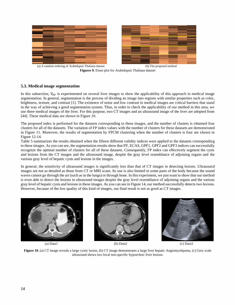
(a) A random ordering of Arabidopsis Thaliana dataset (b) The proposed method

Figures 9. Eisen plot for Arabidopsis Thaliana dataset

5.3. Medical image segmentation

In this subsection, VFP is experimented on several liver images to show the applicability of this approach in medical image

segmentation. In general, segmentation is the process of dividing an image into regions with similar properties such as color,

brightness, texture, and contrast [1]. The existence of noise and low contrast in medical images are critical barriers that stand

in the way of achieving a good segmentation system. Thus, in order to check the applicability of our method in this area, we

use three medical images of the liver. For this purpose, two CT images and an ultrasound image of the liver are adopted from

[44]. These medical data are shown in Figure 10.

The proposed index is performed for the datasets corresponding to these images, and the number of clusters is obtained four

clusters for all of the datasets. The variation of FP index values with the number of clusters for these datasets are demonstrated

in Figure 11. Moreover, the results of segmentation by FPCM clustering when the number of clusters is four are shown in

Figure 12-14.

Table 5 summarizes the results obtained when the fifteen different validity indices were applied to the datasets corresponding

to these images. As you can see, the segmentation results show that FP, ECAS, GPF1, GPF2 and GPF3 indices can successfully

recognize the optimal number of clusters for all of these datasets. Consequently, FP index can effectively segment the cysts

and lesions from the CT images and the ultrasound image, despite the gray level resemblance of adjoining organs and the

various gray level of hepatic cysts and lesions in the images.

In general, the sensitivity of ultrasound images is significantly less than that of CT images in detecting lesions. Ultrasound

images are not as detailed as those from CT or MRI scans. Its use is also limited in some parts of the body because the sound

waves cannot go through the air (such as in the lungs) or through bone. In this experiment, we just want to show that our method

is even able to detect the lesions in ultrasound images despite the gray level resemblance of adjoining organs and the various

gray level of hepatic cysts and lesions in these images. As you can see in Figure 14, our method successfully detects two lesions.

However, because of the low quality of this kind of images, our final result is not as good as CT images.

(a) Data1 (b) Data2 (c) Data3

Figure 10. (a) CT image reveals a large cystic lesion, (b) CT image demonstrates a large liver hepatic Angiomyolipoma, (c) Grey scale

ultrasound shows two focal non-specific hypoechoic liver lesions.

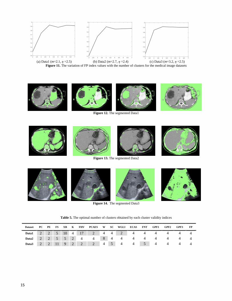
15

(a) Data1 (m=2.1, η =2.5) (b) Data2 (m=2.7, η =2.4) (c) Data3 (m=3.2, η =2.5)

Figure 11. The variation of FP index values with the number of clusters for the medical image datasets

Figure 12. The segmented Data1

Figure 13. The segmented Data2

Figure 14. The segmented Data3

Table 5. The optimal number of clusters obtained by each cluster validity indices

Dataset PC PE FS XB K FHV PCAES W SC WGLI ECAS FNT GPF1 GPF2 GPF3 FP

Data1 2 2 5 10 4 17 2 4 4 2 4 4 4 4 4 4

Data2 2 2 5 5 2 4 4 8 4 4 4 4 4 4 4 4

Data3 2 2 11 9 2 2 2 4 5 4 4 5 4 4 4 4

16

6. Conclusions

In this paper, we reviewed several fuzzy validity indices and discussed their advantages and disadvantages. We observed that

some of them give incorrect results when the cluster centers are close to each other. Moreover, we demonstrated that most of

these indices are susceptible to noise. To tackle these shortcomings, we proposed a new fuzzy-possibilistic validity index called

FP index.

Furthermore, FPCM like other clustering algorithms is susceptible to some initial parameters. In this regard, in addition to the

number of clusters, FPCM requires a priori selection of the degree of fuzziness (m) and the degree of typicality (η). Therefore,

we presented an efficient procedure for determining the optimal values for m and η.

For demonstrating the efficiency of FP index, we examined the proposed index using eight artificial and five well-known

datasets. Our experiments demonstrated the effectiveness and flexibility of the FP validity index regarding sensitivity to cluster

overlapping and difference in cluster shape and density in comparison with several well-known approaches in the literature.

Moreover, we discussed the applications of the proposed approach in real microarray gene expression datasets and medical

image segmentation. In both applications, we observed that our method has an excellent performance in determining the proper

number of clusters, and is robust in the presence of noise.

References [1] Duda, R. O., & Hart, P. E. “Pattern classification and scene analysis” (Vol. 3). New York: Wiley (1973).

[2] Gallegos, M. T., & Ritter, G. “Probabilistic clustering via Pareto solutions and significance tests. Advances in Data Analysis and

Classification”, 12(2), pp. 179-202 (2018).

[3] Bezdek, J. C. “Pattern recognition with fuzzy objective function algorithms”, Springer Science & Business Media (2013).

[4] Krishnapuram, R., & Keller, J. M. “A possibilistic approach to clustering”, IEEE transactions on fuzzy systems, 1(2), pp. 98-110 (1993).

[5] Mendel, J. M. “Type-2 fuzzy sets. In Uncertain Rule-Based Fuzzy Systems”, pp. 259-306, Springer, Cham (2017).

[6] Sotudian, S., Zarandi, M.F. and Turksen, I.B.” From Type-I to Type-II fuzzy system modeling for diagnosis of hepatitis”, World Acad.

Sci. Eng. Technol. Int. J. Comput. Electr. Autom. Control Inf. Eng, 10(7), pp.1238-1246 (2016).

[7] Haldar, N. A. H., Khan, F. A., Ali, A. et al. “Arrhythmia classification using Mahalanobis distance based improved Fuzzy C-Means

clustering for mobile health monitoring systems”, Neurocomputing, 220, pp. 221-235, (2017).

[8] Zarandi, MH Fazel, A. Seifi, H. Esmaeeli et al. “A type-2 fuzzy hybrid expert system for commercial burglary”, In North American Fuzzy

Information Processing Society Annual Conference, pp. 41-51 (2017).

[9] Fazel Zarandi, M. H., Faraji, M. R., and Karbasian, M. “An exponential cluster validity index for fuzzy clustering with crisp and fuzzy

data”, Sci. Iran. Trans. E Ind. Eng, 17, pp. 95-110 (2010).

[10] Wu, K.L., Yang, M.S. “Alternative c-means clustering algorithms”, Pattern Recognition, 35, pp. 2267–2278 (2002).

[11] Dunn, J. C. “A fuzzy relative of the ISODATA process and its use in detecting compact well-separated clusters”, pp. 32-57 (1973).

[12] Krishnapuram, R., and Keller, J. M. “The possibilistic c-means algorithm: insights and recommendations’, IEEE transactions on Fuzzy

Systems, 4(3), pp. 385-393 (1996).

[13] Pal, N. R., Pal, K., and Bezdek, J. C. “A mixed c-means clustering model. In Fuzzy Systems”, Proceedings of 6th International Fuzzy

Systems IEEE, 1, pp. 11-21 (1997).

[14] Wang, W., and Zhang, Y. “On fuzzy cluster validity indices”, Fuzzy sets and systems, 158(19), pp. 2095-2117 (2007).

[15] Bezdek, J. C., Keller, J., Krisnapuram, R. et al. “Fuzzy models and algorithms for pattern recognition and image processing”, Springer

Science and Business Media, (2006).

[16] Wijayasekara, D., Linda, O., and Manic, M. “Shadowed Type-2 Fuzzy Logic Systems”, In T2FUZZ , pp. 15-22 (2013).

[17] Fukuyama, Y., and Sugeno, M. “A new method of choosing the number of clusters for the fuzzy c-means method”, In Proc. 5th Fuzzy

Syst. Symp, (247), pp. 247-250 (1989).

[18] Xie, X. L., and Beni, G. “A validity measure for fuzzy clustering”, IEEE Transactions on pattern analysis and machine intelligence,

13(8), pp. 841-847(1991).

[19] Kwon, S.H. “Cluster validity index for fuzzy clustering”, Electron Lett., 34(22), pp. 2176-2178 (1998).

[20] Gath, I., and Geva, A. B. “Unsupervised optimal fuzzy clustering”, IEEE Transactions on pattern analysis and machine intelligence,

11(7), pp. 773-780 (1989).

[21] Wu, K. L., & Yang, M. S. “A cluster validity index for fuzzy clustering”, Pattern Recognition Letters, 26(9), pp. 1275-1291(2005).

[22] Zhang, Y., Wang, W., Zhang, X. et al. “A cluster validity index for fuzzy clustering”, Information Sciences, 178(4), pp. 1205-1218

(2008).

[23] Rezaee, B “A cluster validity index for fuzzy clustering”, Fuzzy Sets and Systems, 161(23), pp. 3014-3025 (2010).

[24] Zhang, D., Ji, M., Yang, J. et al. “A novel cluster validity index for fuzzy clustering based on bipartite modularity”, Fuzzy Sets and

Systems, 253, pp. 122-137 (2014).

[25] Zarandi, M. H. F., Neshat, E., and Türkşen, I. B. “Retracted Article: A New Cluster Validity Index for Fuzzy Clustering Based on

Similarity Measure”, In International Workshop on Rough Sets, Fuzzy Sets, Data Mining, and Granular-Soft Computing,Springer, Berlin,

Heidelberg, pp. 127-135 (2007).

17

[26] Askari, S., Montazerin, N., & Zarandi, M. F. “Generalized Possibilistic Fuzzy C-Means with novel cluster validity indices for clustering

noisy data”, Applied Soft Computing, 53, pp. 262-283 (2017).

[27] Pal, N. R., and Pal, S. K. “Entropy: A new definition and its applications”, IEEE transactions on systems, man, and cybernetics, 21(5),

pp. 1260-1270 (1991).

[28] Pal, N. R., and Pal, S. K. “Some properties of the exponential entropy”, Information sciences, 66(1-2), pp. 119-137(1992).

[29] Bezdek, J. C. “Pattern Recognition with Fuzzy Objective Algorithms”, Plenum Press, New York. (1981).

[30] McBratney, A. B., and Moore, A. W. “Application of fuzzy sets to climatic classification”, Agricultural and forest meteorology, 35(1-

4), pp. 165-185 (1985).

[31] Choe, H., and Jordan, J. B. “On the optimal choice of parameters in a fuzzy c-means algorithm”, IEEE International Conference on

Fuzzy Systems, pp. 349-354 (1992).

[32] Yu, J., Cheng, Q., and Huang, H. “Analysis of the weighting exponent in the FCM”, IEEE Transactions on Systems, Man, and

Cybernetics, Part B (Cybernetics), 34(1), pp. 634-639 (2004).

[33] Okeke, F., and Karnieli, A. “Linear mixture model approach for selecting fuzzy exponent value in fuzzy c-means algorithm”, Ecological

Informatics, 1(1), pp. 117-124 (2006).

[34] Bezdek, J.C. “Pattern Recognition in Handbook of Fuzzy Computation”, IOP Publishing Ltd., Boston, MA, (1998),

[35] UCI Machine Learning Repository, Retrieved October 21, 2018, from http://www.ics.uci.edu/~mlearn/databases.html.

[36] Torshizi, A. D., Zarandi, M. F., and Türksen, I. B. “Computing centroid of general type-2 fuzzy set using constrained switching

algorithm”, Scientia Iranica, Transaction E, Industrial Engineering, 22(6), p 2664 (2015).

[37] Jothi, R., Sraban Kumar Mohanty, and Aparajita Ojha. "DK-means: a deterministic K-means clustering algorithm for gene expression

analysis", Pattern Analysis and Applications, pp. 1-19 (2017).

[38] Hosseini, Behrooz, and Kourosh Kiani. "FWCMR: A scalable and robust fuzzy weighted clustering based on MapReduce with

application to microarray gene expression", Expert Systems with Applications 91, pp. 198-210 (2018).

[39] Jiang, Daxin, Chun Tang, and Aidong Zhang. "Cluster analysis for gene expression data: a survey", IEEE Transactions on knowledge

and data engineering. 16(11), pp. 1370-1386 (2004).

[40] The Transcriptional Program of Sporulation in Budding Yeast. (n.d.). Retrieved October 21, 2018, from

http://www.sciencemag.org/content/282/5389/699.long

[41] Validating Clustering for Gene Expression Data. (n.d.). Retrieved October 21, 2018, from http://faculty.washington.edu/ kayee/cluster.

[42] Biological Data Analysis using Clustering. (n.d.). Retrieved October 21, 2018, from http://homes.esat.kuleuven.be/~thijs

Work/Clustering.html

[43] Eisen, M. B., Spellman, P. T., Brown, P. O., and Botstein, D. “Cluster analysis and display of genome-wide expression patterns”,

Proceedings of the National Academy of Sciences, 95(25), pp. 14863-14868 (1998).

[44] Open-edit radiology resource, Retrieved October 21, 2018, from http:// Radiopaedia.org.