A novel MAP-MRF approach for multispectral image contextual classification using combination of suboptimal iterative algorithms

Pattern Recognition Letters 31 (2010) 1795–1808

Contents lists available at ScienceDirect

Pattern Recognition Letters

journal homepage: www.elsevier .com/locate /patrec

A novel MAP-MRF approach for multispectral image contextual classificationusing combination of suboptimal iterative algorithms

Alexandre L.M. Levada a,*, Nelson D.A. Mascarenhas b, Alberto Tannús a

a Physics Institute of São Carlos, University of São Paulo, São Carlos, SP, Brazilb Computing Department, Federal University of São Carlos, São Carlos, SP, Brazil

a r t i c l e i n f o

Article history:Available online 10 April 2010

Keywords:Contextual classificationMarkov random fieldsCombinatorial optimizationMaximum pseudo-likelihoodData fusionClassifier combination

0167-8655/$ - see front matter � 2010 Elsevier B.V. Adoi:10.1016/j.patrec.2010.04.007

* Corresponding author. Tel.: +55 19 35410627; faxE-mail address: [email protected] (A.L.

a b s t r a c t

In this paper we present a novel approach for multispectral image contextual classification by combiningiterative combinatorial optimization algorithms. The pixel-wise decision rule is defined using a Bayesianapproach to combine two MRF models: a Gaussian Markov Random Field (GMRF) for the observations(likelihood) and a Potts model for the a priori knowledge, to regularize the solution in the presence ofnoisy data. Hence, the classification problem is stated according to a Maximum a Posteriori (MAP) frame-work. In order to approximate the MAP solution we apply several combinatorial optimization methodsusing multiple simultaneous initializations, making the solution less sensitive to the initial conditionsand reducing both computational cost and time in comparison to Simulated Annealing, often unfeasiblein many real image processing applications. Markov Random Field model parameters are estimated byMaximum Pseudo-Likelihood (MPL) approach, avoiding manual adjustments in the choice of the regular-ization parameters. Asymptotic evaluations assess the accuracy of the proposed parameter estimationprocedure. To test and evaluate the proposed classification method, we adopt metrics for quantitativeperformance assessment (Cohen’s Kappa coefficient), allowing a robust and accurate statistical analysis.The obtained results clearly show that combining sub-optimal contextual algorithms significantlyimproves the classification performance, indicating the effectiveness of the proposed methodology.

� 2010 Elsevier B.V. All rights reserved.

1. Introduction

Undoubtedly, Markov Random Fields (MRF) define a powerfulmathematical tool for contextual modeling of spatial data. Withadvances in probability and statistics (Hammersley and Clifford,1971), as the development of Markov Chain Monte Carlo (MCMC)simulation techniques (Metropolis et al., 1953; Geman and Geman,1984; Swendsen and Wang, 1987; Wolff, 1989) and relaxationalgorithms for combinatorial optimization (Besag, 1986; Marro-quin et al., 1987; Blake and Zisserman, 1987; Nikolova et al.,1998; Chou and Brown, 1990; Yu and Berthod, 1995), MRF’s be-came a central topic in fields including image processing, computervision and pattern recognition (Li and Peng, 2004; Richard, 2005;Bentabet and Maodong, 2008; Cariou and Chehdi, 2008). In this pa-per, we are concerned with the multispectral image contextualclassification problem using a MAP-MRF Bayesian framework thatcombines two MRF models: a Gaussian Markov Random Field(GMRF) for the observations (likelihood) and a Potts model as asmooth prior, acting as a regularization term in the presence ofnoisy data, by reducing the solution space.

ll rights reserved.

: +55 16 33518233.M. Levada).

It is widely known that the solution for MAP-MRF based clas-sification problems requires the use of iterative combinatorialoptimization algorithms. One of these algorithms, known asSimulated Annealing (SA) have been proven to be optimal (Gemanand Geman, 1984), since it slowly converges to the global opti-mum after a large number of iterations, regardless the initial con-ditions. However, it is also know that SA has some majordrawbacks: besides its high computational cost, SA convergencerate is extremely low, making it unfeasible to several real worldapplications.

To avoid this problem with SA computational cost and conver-gence, several sub-optimal combinatorial optimization algorithmswere proposed in literature, among which we can cite the widelyrecognized Besag’s Iterated Conditional Modes (ICM) (Besag, 1986),Maximizer of the Posterior Marginals (MPM) (Marroquin et al.,1987), Graduated Non-Convexity (GNC) (Blake and Zisserman,1987), Highest Confidence First (HCF) (Chou and Brown, 1990) andGame Strategy Approach (GSA) (Yu and Berthod, 1995), an algo-rithm based on non-cooperative game theory (Nash, 1950). For in-stance, in (Dubes and Jain, 1989) it has been reported that, inrelative terms, MPM can be more than one hundred times fasterthan SA while ICM can reach the impressive mark of more thanone thousand times faster than SA, showing a huge difference on

http://dx.doi.org/10.1016/j.patrec.2010.04.007

mailto:[email protected]

http://www.sciencedirect.com/science/journal/01678655

http://www.elsevier.com/locate/patrec

1796 A.L.M. Levada et al. / Pattern Recognition Letters 31 (2010) 1795–1808

the computational times. However, despite their apparent advan-tages, these sub-optimal algorithms also have some drawbacks:strong dependence on the initial conditions and convergence onlyto local maxima/minima.

Thus, to attenuate these intrinsic sub-optimal algorithms limi-tations, aiming an improvement in classification performance,but at the same time keeping a reasonable computational cost,we propose a novel approach for combining contextual classifiers.The basic idea consists of using multiple simultaneous initializa-tions and classifier combination strategies (Kittler et al., 1998;Kuncheva, 2004; Valev and Asaithambi, 2001; Alexandre et al.,2001; Aksela and Laaksonen, 2007; Lam and Suen, 1995; Kin andOh, 2008) to make the final solution less sensitive to the initialconditions.

Usually, in Bayesian inference, more precisely, in MAP-MRF ap-proaches, the prior probability is given by a Markovian model. Inthis scenario, the MRF model parameter assumes the role of a reg-ularization parameter, since it controls the tradeoff between theprior knowledge and the likelihood. However, in most contextualclassification systems, MRF model parameters are still chosen bya trial-and-error procedure through simple manual adjustments(Solberg, 2004; Wu and Chung, 2007). In this work, we use pseu-do-likelihood equations to estimate the MRF parameters (Levadaet al., 2008). It has been shown that MPL estimation is computa-tionally feasible and from an statistical perspective, it has a seriesof desirable and useful properties, such as consistency and asymp-totic normality (Jensen and Künsh, 1994; Winkler, 2006). Besides,the derivation of an approximation for the asymptotic variance ofMPL estimators allows us to assess the accuracy of MRF parameterestimation, as well as to do inferences about the MRF modelparameters through hypothesis testing (Levada et al., 2008). In thissense, in our MAP-MRF approach, the estimated MRF parametersare the best ones based on the available observed data and themain advantage is that they do not need to be manually chosenby the end-user.

In this work, our main contributions are twofold. Concerningthe multispectral image contextual classification, this is, to thebest of our knowledge, the first time a combination of iterativesuboptimal combinatorial optimization algorithms is performedby making use of multiple initializations and classifier combina-tion rules. A second issue that is worth mentioning is that theMarkov Random Field model parameters were estimated by Max-imum Pseudo-Likelihood (MPL) approach, allowing us to auto-matically define the regularization parameter, avoiding manualadjustments by simple trial-and-error, a situation that is stillusual in practice.

The remaining of the paper is organized as follows: Section 2introduces the MAP-MRF contextual classification model. Section3 discusses the MRF parameter estimation stage by showing pseu-do-likelihood equations for the proposed MAP-MRF model param-eters. Section 4 presents approximations for the asymptoticvariances of both GMRF and Potts MPL estimators, assessing theaccuracy of the parameter estimation procedure. Section 5 showssome rules for information fusion and metrics for quantitative per-formance evaluation. Section 6 shows the experimental setup,describing the obtained results. Finally, Section 7 presents the con-clusions and final remarks.

2. MAP-MRF contextual classification

Basically, the proposed methodology for combining contextualclassifiers follows the block diagram illustrated in Fig. 1. Given amultispectral image as input, the first step consists in defining bothspectral (likelihood) and spatial (MRF prior) statistical models.After that, the definition of training and test sets is necessary since

we are dealing with supervised classification. From the training set,the class conditional densities parameter estimation is performed.Eventually, some feature extraction method may be required to re-duce the dimensionality of the classification problem. At this point,we have the initialization stage, where several pattern classifiersare used to generate different initial conditions for the sub-optimaliterative combinatorial optimization algorithms (ICM, GSA andMPM). A lot of classification methods can be applied in the gener-ation of the initializations, from neural network based classifiers toSupport Vector Machines (SVM). In this work we selected sevenstatistical pattern classifiers: Linear and Quadratic Bayesian classi-fiers (under Gaussian hypothesis), Parzen-Windows classifier, K-Nearest-Neighbor classifier, Logistic classifier, Nearest Mean classi-fier and a Decision-Tree classifier. An extensive literature on pat-tern classifiers can be found in (Fukunaga, 1990; Duda et al.,2001; Webb, 2002; Theodoridis and Koutroumbas, 2006). The iter-ative combinatorial optimization algorithms improve the initialsolutions by making use of the MRF parameters estimated by theproposed MPL approach. Finally, the classifier combination stageis responsible for the data fusion by incorporating informationfrom different contextual observations in the decision making pro-cess using six rule-based combiners: Sum, Product, Maximum, Min-imum, Median and Majority Vote (Kittler et al., 1998; Kuncheva,2004).

The iterative contextual classification is achieved by updatingeach image pixel by a new label that maximizes the posterior dis-tribution. Let xðpÞW be the label field at the pth iteration, y the ob-served multispectral image, h = [h1,h2,h3,h4] the 4D vector ofGMRF hyperparameters (directional spatial dependency parame-ters), / the vector of GMRF spectral parameters for each class(lm,Rm) and b the Potts model hyperparameter (regularizationparameter). Considering a multispectral GMRF model for theobservations and a Potts model for the a priori knowledge, accord-ing to the Bayes’ rule, the current label of pixel (i, j) can be updatedby choosing the label that maximizes the functional (Yamazaki andGingras, 1996):

Q xij ¼m xðpÞW ;y;h;/;b��

¼�12

ln bRm

�� 1

2yij � lm

bHT ygij� 2

Xct

hct

!lm

" #( )T

� bR�1m � yij � lm

bHT ygij� 2

Xct

hct

!lm

" #( )þ bUijðmÞ; ð1Þ

where hct is a diagonal matrix whose elements are the horizontal,vertical and diagonals hyperparameters (4 � 4), ct = 1, . . . ,K,where K is the number of bands, hT is a matrix built by stackingthe bHct diagonal matrices from each image band (4 � 4K), that is,bHT ¼ ½hct1; hct2; . . . ; hctK � and ygij

is a vector whose elements are de-fined as the sum of the two neighboring elements on each direc-tion (horizontal, vertical, and diagonals) for all the image bands(4K � 1). Basically, this decision rule works as follows: in caseof extremelly noisy situations, no confidence is placed in the con-textual information, since b is small and the decision is mademostly because of the likelihood term. On the other side, whencontextual information is informative, that is, b is significant, spa-tial information is considered in the decision rule. It is worth-while to note that in this context, the Potts model b parametercontrols the tradeoff between spectral and spatial information,that is, data fidelity and prior knowledge, so its correct settingis crucial for the classification performance. This double-MRFmodel was originally proposed by Yamazaki and Gingras (1996),however it was restricted to first-order beighborhood systems.

Fig. 1. Block diagram of the proposed multispectral image contextual classification system using combination of sub-optimal iterative combinatorial optimizationalgorithms.

A.L.M. Levada et al. / Pattern Recognition Letters 31 (2010) 1795–1808 1797

Here, besides extending this compound model to second-ordersystems, we use a novel pseudo-likelihood equation for Potts

model parameter estimation and combination of multiple contex-tual classifiers.


3. MRF parameter estimation

One of the main difficulties in contextual classification using aMAP-MRF approach relies on the MRF parameter estimation stage.Traditional methods, as Maximum Likelihood (ML), cannot be ap-plied due to the existence of a partition function in the joint Gibbsdistribution, which is computationally intractable. A solution pro-posed by Besag to surmount this problem is to use the local condi-tional density functions (LCDF) to perform maximum pseudo-likelihood (MPL) estimation (Besag, 1974). The main motivationfor employing this approach is that MPL estimation is a computa-tionally feasible method. Besides, from a statistical perspective,MPL estimators have a series of desirable and interesting proper-ties, such as consistency and asymptotic normality (Jensen andKünsh, 1994). In this section, pseudo-likelihood equations for bothGMRF and Potts models are presented and their accuracy are as-sessed using asymptotic evaluations and MCMC simulationalgorithms.

3.1. MPL estimation for GMRF model parameters

As the proposed model for contextual classification of multi-spectral images assumes that the image bands are uncorrelated,it is quite reasonable to perform MPL estimation in each imageband separately. Assuming this hypothesis and considering a sec-ond-order neighborhood system, the pseudo-likelihood equationfor the GMRF hyperparameters becomes (Won and Gray, 2004):

log PLðh;l;r2Þ ¼Xði;jÞ2W

�12

logð2pr2Þ � 12r2 yij � hwij

��l 1� 2huð Þ�2

o; ð2Þ

where W represents an image band, u = [1,1,1,1]T is the 4D identityvector and both h (GMRF directional hyperparameters vector) andwij (a 4D vector where each element is the sum of the neighboringpixels around (i,j) in each direction) are defined as:

h ¼ ½h1; h2; h3; h4�; ð3Þwij ¼ ½ðyiþ1;j þ yi�1;jÞ; ðyi;jþ1 þ yi;j�1Þ; ðyiþ1;j�1 þ yi�1;jþ1Þ;

ðyi�1;j�1 þ yiþ1;jþ1Þ�T: ð4Þ

Fortunately, the MPL estimator of h admits a closed solution, givenby Won and Gray (2004):

h ¼Xði;jÞ2W

yij � l� �

~wTij

" # Xði;jÞ2W

~wij~wT

ij

" #�18<:

9=;; ð5Þ

where l is the sample mean of the image pixels, ~wij ¼wij � 1

N

Pðk;lÞ2Wwij and N is the number of image pixels. Finally, for

the class conditional GMRF spectral parameters we use the tradi-tional maximum likelihood estimators: the sample mean and thesample covariance matrix.

3.2. MPL estimation for Potts MRF model parameter

One of the most widely used prior models in Bayesian imagemodelling is the Potts MRF pair-wise interaction (PWI) model.Basically, the Potts model tries to represent the way individual ele-ments (e.g., atoms, animals, image pixels, etc.) modify their behav-ior to conform to the behavior of other individuals in their vicinity.It is a model used to study collective effects based on consequencesof local interactions. It has a major role in several research areassuch as mathematics (Wu, 1992; Adams, 1994; Ge et al., 1996;Jin and Zhang, 2004), physics (Montroll, 1941; Enting and Gutt-mann, 2003), biology (Ouchi et al., 2003; Merks and Glazier,

2005) and computer science (Berthod et al., 1995; Won and Gray,2004; Farag et al., 2005).

Two fundamental characteristics of the Potts model consideredhere are: it is both isotropic and stationary. According to Ham-mersley and Clifford (1971), the Potts MRF model can be equiva-lently defined in two manners: by a joint Gibbs distribution(global model) or by a set of local conditional density functions(LCDF’s). For a general sth order neighborhood system gs, we definethe former by the following expression:

pðxij ¼ mijjgsijÞ ¼

expfbUijðmijÞgPM‘¼1 expfbUijð‘Þg

; ð6Þ

where Uij(‘) is the number of neighbors of the (i,j)th element havinglabel equal to ‘,b is the spatial dependency parameter (also knownas inverse temperature), mij, l 2 G = {1,2, . . . ,M}, with M denotingthe number of classes. Briefly speaking, the notion of order is di-rectly related to the extension of the neighborhood system. For in-stance, the two most widely known neighborhood systems, formedby the four and eight nearest neighbors, are known as first and sec-ond-order systems, respectively.

In the following, we briefly describe the pseudo-likelihoodequations proposed in Levada et al. (2008). Asymptotic evaluationsusing approximations for the variance of these estimators showthat the proposed equations are valid and accurate (Levada et al.,2008,), providing a robust method for automatic definition of theregularization parameter used in MAP-MRF approaches.

The pseudo-likelihood equation for the Potts model is given by:

PLðbÞ ¼Yði;jÞ2W

pðxij ¼ mijjgsijÞ ¼

Yði;jÞ2W

expfbUijðmijÞgPM‘¼1 expfbUijð‘Þg

: ð7Þ

Taking the logarithms, differentiating on the parameter and settingthe result to zero, leads to the following expression, which is the ba-sis for the derivation of the proposed pseudo-likelihood equation:

WðbÞ ¼ @

@blogPLðbÞ

¼Xði;jÞ2W

UijðmijÞ �Xði;jÞ2W

PM‘¼1Uijð‘Þ expfbUijð‘ÞgPM

‘¼1 expfbUijð‘Þg

" #¼ 0; ð8Þ

where mij denotes the observed value for the (i, j)th element of thefield.

Basically, the derivation of the Potts model pseudo-likelihoodequation consists in expanding the second term of Eq. (8) in allpossible spatial configuration patterns that provide different con-tributions to the pseudo-likelihood function, regarding a pre-de-fined neighborhood system, in this case a second-order system.For example, in first order systems, the enumeration of these con-figuration patterns is straightforward, since there are only fivecases, from zero agreement (case of four different labels) to totalagreement (case of four identical labels), as shown in Fig. 2.

These configuration patterns can represented by vectors, as pre-sented in relations (7), indicating the number of occurrences ofeach element around the central element. In the Potts model loca-tion information is irrelevant since it is an isotropic model:

v0 ¼ ½1;1;1;1� v1 ¼ ½2;1;1;0� v2 ¼ ½2;2;0;0�v3 ¼ ½3;1;0;0� v4 ¼ ½4;0;0;0�: ð9Þ

Let N be the number of elements in the neighborhood system gs. Foreach L = 1,2, . . . ,N let:

ANðLÞ ¼�ða1; . . . ; aLÞ=ai 2 f1; 2; . . . ; Ng; a1 6 a2 6 � � � 6 aL;

XL

i¼1

ai ¼ N

ð10Þ

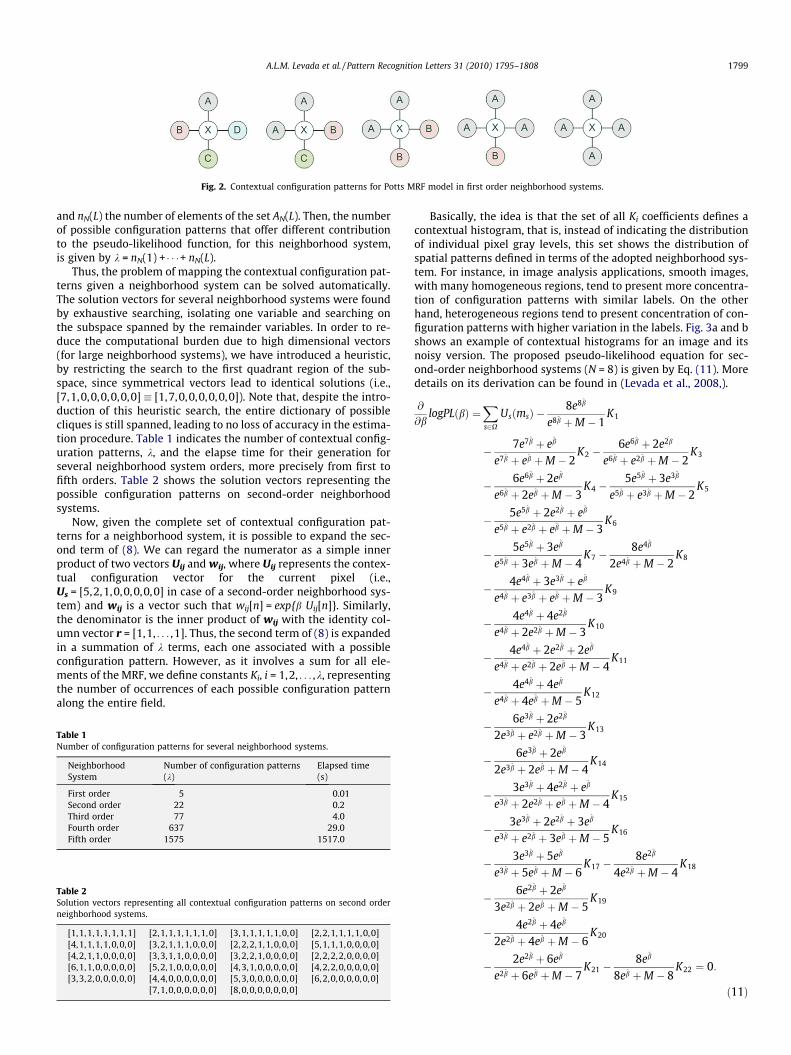
Fig. 2. Contextual configuration patterns for Potts MRF model in first order neighborhood systems.


and nN(L) the number of elements of the set AN(L). Then, the numberof possible configuration patterns that offer different contributionto the pseudo-likelihood function, for this neighborhood system,is given by k = nN(1) + � � �+ nN(L).

Thus, the problem of mapping the contextual configuration pat-terns given a neighborhood system can be solved automatically.The solution vectors for several neighborhood systems were foundby exhaustive searching, isolating one variable and searching onthe subspace spanned by the remainder variables. In order to re-duce the computational burden due to high dimensional vectors(for large neighborhood systems), we have introduced a heuristic,by restricting the search to the first quadrant region of the sub-space, since symmetrical vectors lead to identical solutions (i.e.,[7,1,0,0,0,0,0,0] � [1,7,0,0,0,0,0,0]). Note that, despite the intro-duction of this heuristic search, the entire dictionary of possiblecliques is still spanned, leading to no loss of accuracy in the estima-tion procedure. Table 1 indicates the number of contextual config-uration patterns, k, and the elapse time for their generation forseveral neighborhood system orders, more precisely from first tofifth orders. Table 2 shows the solution vectors representing thepossible configuration patterns on second-order neighborhoodsystems.

Now, given the complete set of contextual configuration pat-terns for a neighborhood system, it is possible to expand the sec-ond term of (8). We can regard the numerator as a simple innerproduct of two vectors Uij and wij, where Uij represents the contex-tual configuration vector for the current pixel (i.e.,Us = [5,2,1,0,0,0,0,0] in case of a second-order neighborhood sys-tem) and wij is a vector such that wij[n] = exp{b Uij[n]}. Similarly,the denominator is the inner product of wij with the identity col-umn vector r = [1,1, . . . ,1]. Thus, the second term of (8) is expandedin a summation of k terms, each one associated with a possibleconfiguration pattern. However, as it involves a sum for all ele-ments of the MRF, we define constants Ki, i = 1,2, . . . ,k, representingthe number of occurrences of each possible configuration patternalong the entire field.

Table 1Number of configuration patterns for several neighborhood systems.

NeighborhoodSystem

Number of configuration patterns(k)

Elapsed time(s)

First order 5 0.01Second order 22 0.2Third order 77 4.0Fourth order 637 29.0Fifth order 1575 1517.0

Table 2Solution vectors representing all contextual configuration patterns on second orderneighborhood systems.

[1,1,1,1,1,1,1,1] [2,1,1,1,1,1,1,0] [3,1,1,1,1,1,0,0] [2,2,1,1,1,1,0,0][4,1,1,1,1,0,0,0] [3,2,1,1,1,0,0,0] [2,2,2,1,1,0,0,0] [5,1,1,1,0, 0,0,0][4,2,1,1,0,0,0, 0] [3,3,1,1,0,0,0,0] [3,2,2,1,0,0,0,0] [2,2,2,2,0, 0,0,0][6,1,1,0,0,0,0,0] [5,2,1,0,0,0, 0,0] [4,3,1,0,0,0, 0,0] [4,2,2,0,0,0,0, 0][3,3,2,0,0,0,0,0] [4,4,0,0,0,0,0,0] [5,3,0,0,0,0,0,0] [6,2,0,0,0,0,0,0]

[7,1,0,0,0,0,0,0] [8,0,0,0,0,0,0,0]

Basically, the idea is that the set of all Ki coefficients defines acontextual histogram, that is, instead of indicating the distributionof individual pixel gray levels, this set shows the distribution ofspatial patterns defined in terms of the adopted neighborhood sys-tem. For instance, in image analysis applications, smooth images,with many homogeneous regions, tend to present more concentra-tion of configuration patterns with similar labels. On the otherhand, heterogeneous regions tend to present concentration of con-figuration patterns with higher variation in the labels. Fig. 3a and bshows an example of contextual histograms for an image and itsnoisy version. The proposed pseudo-likelihood equation for sec-ond-order neighborhood systems (N = 8) is given by Eq. (11). Moredetails on its derivation can be found in (Levada et al., 2008,).

@

@blogPLðbÞ ¼

Xs2X

UsðmsÞ �8e8b

e8b þM � 1K1

� 7e7b þ eb

e7b þ eb þM � 2K2 �

6e6b þ 2e2b

e6b þ e2b þM � 2K3

� 6e6b þ 2eb

e6b þ 2eb þM � 3K4 �

5e5b þ 3e3b

e5b þ e3b þM � 2K5

� 5e5b þ 2e2b þ eb

e5b þ e2b þ eb þM � 3K6

� 5e5b þ 3eb

e5b þ 3eb þM � 4K7 �

8e4b

2e4b þM � 2K8


e4b þ e3b þ eb þM � 3K9

� 4e4b þ 4e2b

e4b þ 2e2b þM � 3K10

� 4e4b þ 2e2b þ 2eb

e4b þ e2b þ 2eb þM � 4K11

� 4e4b þ 4eb

e4b þ 4eb þM � 5K12

� 6e3b þ 2e2b

2e3b þ e2b þM � 3K13

� 6e3b þ 2eb

2e3b þ 2eb þM � 4K14


e3b þ 2e2b þ eb þM � 4K15

� 3e3b þ 2e2b þ 3eb

e3b þ e2b þ 3eb þM � 5K16

� 3e3b þ 5eb

e3b þ 5eb þM � 6K17 �

8e2b

4e2b þM � 4K18

� 6e2b þ 2eb


� 4e2b þ 4eb


� 2e2b þ 6eb

e2b þ 6eb þM � 7K21 �

8eb

8eb þM � 8K22 ¼ 0:

ð11Þ

Fig. 3. Comparison between the distribution of typical contextual configuration patterns for a smooth and a noisy image (k0 stands for total agreement and k22 for zeroagreement).


We would like to emphasize three important points about theproposed equation. First, it can be seen that each one of the 22terms is composed by a product of two factors: a fraction and aKi value. The first factor is nothing more than the contribution ofthe respective contextual configuration pattern to the pseudo-like-lihood equation, while the second one is the number of times thispattern occurs along the image. Another important issue is relatedto the validity of the proposed equation for an arbitrary M (numberof classes or states). For a reduced number of classes (tipically,M = 3, M = 4), the equation is further simplified, since many Ki

0s,

i = 1,2, . . . ,k, are zero, simply because many contextual patternsare physically impossible to occur. Therefore, in practical terms, areduction on the number of clasees in the classification problem(M) implies in reduction of the computational cost of the PottsMRF model parameter estimation. Finally, it is worthwhile to notethat symmetrical configuration patterns offer the same contribu-tion to the pseudo-likelihood equation, since the inner product be-tween two vectors does not depend of the order of the elements.

The derived transcendental equations do not have closed solu-tion, so in order to solve them a root-finding algorithm is required.In all experiments along this chapter, the MPL estimator is ob-tained by Brent’s method (Brent, 1973), a numerical method thatdoes not require the computation (not even the existence) of deriv-atives or analytical gradients. In this case, the computation ofderivatives of the objective function would be prohibitive, giventhe large extension of the expressions. Basically, the advantagesof this method can be summarized by: it uses a combination ofbisection, secant and inverse quadratic interpolation methods,leading to a very robust approach and also it has super-linear con-vergence rate.

4. Statistical inference and asymptotic evaluation on Markovrandom fields

As we have seen from previous sections, the choice of the regu-larization parameter (b) plays an important role in the proposedclassification method. Many papers report that this parameter isstill chosen manually, by simple trial-and-error, in a variety ofapplications. The main reason for this usual practice is that,although widely applied in practical problems, little is knownabout the accuracy of maximum pseudo-likelihood estimation. Inthis section, we provide approximations for the asymptotic vari-ance of MPL estimators, assessing the accuracy of the proposedMPL equation for Potts model parameter estimation.

It has been reported in statistical inference theory that unbi-asedness is not granted by maximum pseudo-likelihood (MPL)estimation. However, similarly to maximum likelihood, MPL esti-mation possesses several attractive and desirable statistical prop-erties, such as consistency and asymptotic normality (Jensen andKünsh, 1994; Winkler, 2006). In this work, we used approxima-tions for the asymptotic variances of these estimators for bothPotts and GMRF models derived in (Levada et al., 2008) to assessthe accuracy of MRF parameter estimation.

4.1. On the asymptotic variances of GMRF model MPL estimators

The asymptotic covariance matrix for MPL estimators is givenby Liang and Yu (2003):

CðhÞ ¼ H�1ðhÞJðhÞH�1ðhÞ; ð12Þ

where J(h) and H(h) are functions of the Jacobian (first order partialderivatives) and Hessian (second order partial derivatives) matrices,respectively:

HðhÞ ¼ E½r2logPLðhÞ�; ð13ÞJðhÞ ¼ Var½rlogPLðhÞ�: ð14Þ

Considering that the GMRF hyperparameters h1, h2, h3, h4 are uncor-related (diagonal covariance matrix), and using the observed Fisherinformation (Efron and Hinkley, 1978; Casella and Berger, 2002;Lehmann, 1983; Bickel, 1991) it is possible to approximate theasymptotic variances of the MPL estimators by Levada et al. (2008):

ckkðhÞ ¼bI1

obsðhÞbI2obsðhÞ

h i2 ; k ¼ 1; . . . ;4; ð15Þ

where

bI1obsðhÞ ¼

1Nr4

XN

i¼1

yij � hwij � l 1� 2huð Þ�

wkij � 2l

h in o2ð16Þ

bI2obsðhÞ ¼ �

1Nr2

XN

i¼1

wkij � 2l

h i2ð17Þ

and wkij denotes the kth element of the 4D vector wij,k = 1, . . . ,4, de-

fined in Eq. (4).The proposed approximation allows the calculation of the

asymptotic variance of maximum pseudo-likelihood estimatorsof the GMRF model in computationally feasible way. From previous

Table 3MPL estimators, asymptotic variances and 90% confidence intervals for GMRFhyperparameters on simulated images (Fig. 4a).

K hk hk rk 90% IC

1 0.25 0.2217 0.0390 [0.1799 0.3077]2 0.3 0.2758 0.0387 [0.2398 0.3667]3 �0.1 �0.1145 0.0394 [�0.1771 �0.0479]4 0.2 0.1743 0.0386 [0.1150 0.2416]

Table 4MPL estimators, asymptotic variances and 90% confidence intervals for GMRFhyperparameters on simulated images (Fig. 4b).

K hk hk rk 90% IC

1 0.2 0.1908 0.0506 [0.1079 0.2738]2 0.15 0.1605 0.0524 [0.0746 0.2464]3 0.07 0.0716 0.0482 [�0.0074 0.1506]4 0.05 0.0523 0.0418 [�0.0146 0.1192]


works on statistical inference it can be shown that MPL estimatorsare asymptotically normal distributed. Therefore, with the pro-posed method, it is possible to completely characterize the asymp-totic behavior of the MPL estimators of the GMRF model, allowinginterval estimation, hypothesis testing and quantitative analysis onthe model parameters in a variety of research areas, including im-age processing and pattern recognition (Levada et al., 2008,; Mar-tins et al., 2009).

In order to demonstrate the application of the asymptotic vari-ance estimation in stochastic image modeling, we present the re-sults obtained in experiments using Markov Chain Monte Carlosimulation methods (Dubes and Jain, 1989; Winkler, 2006) bycomparing the values of hMPL and asymptotic variances regardingsecond order neighborhood systems using synthetic images, repre-senting several GMRF model outcomes. For the experiments below,we adopted the Metropolis algorithm (Metropolis et al., 1953), asingle spin flip MCMC method, to simulate occurrences of GRMFmodel using different known parameter vectors. Simulated imagesare shown in Fig. 4. The MPL estimators, obtained by (15) werecompared with the real parameter vectors. In all cases, the param-eters l and r2 were defined as zero and five, respectively. The vec-tor parameters used in the simulated images wereh = [0.25,0.3,0.1,0.2] and h = [0.2,0.15,0.07,0.05].

Table 3 shows the MPL estimators, estimated asymptotic vari-ances, 90% confidence intervals regarding the GMRF model param-eters for the synthetic image indicated in Fig. 4a. Similarly, Table 4shows the same obtained results for the images shown in Fig. 4b.The results on MCMC simulation images show that, in all cases,the true parameter value is contained in the obtained intervals,assessing the accuracy of the proposed methodology for asymp-totic variance estimation.

4.1.1. On the asymptotic variance of Potts MRF model MPL estimatorSimilarly to the GMRF model, it is possible to define an approx-

imation for the asymptotic variance of Potts model MPL estimatorsby deriving expressions for bI1

obsðbÞ and bI2obsðbÞ. From the LCDF of the

Potts model (6), and after some algebraic manipulations, we have(Levada et al., 2008):

bI1obsðbÞ ¼

1N

XN

i¼1

�PM

‘¼1

PMk¼1ðUiðmiÞ �Uið‘ÞÞðUiðmiÞ�UiðkÞÞebðUið‘ÞþUiðkÞÞ

h iPM

‘¼1ebUið‘Þh i2

8><>:9>=>;ð18Þ

where N denotes the number of image pixels and M is the numberof classes.

Fig. 4. Synthetic images generated by MCMC simulation for G

Calculating the observed Fisher information using the secondderivative of the pseudo-likelihood function leads to the following(Levada et al., 2008):

bI2obsðbÞ ¼

1N

XN

i¼1

PM�1‘¼1

PMk¼‘þ1ðUið‘Þ � UiðkÞÞ2ebðUið‘ÞþUiðkÞÞ

h iPM

‘¼1ebUið‘Þh i2

8><>:9>=>; ð19Þ

This approximation allows the calculation of the asymptotic vari-ance of the maximum pseudo-likelihood estimator of the PottsMRF model. In order to demonstrate the application of the asymp-totic variance in testing and evaluating the proposed pseudo-likeli-hood equation, some results obtained in simulations are presented.The results show the values of bMPL, asymptotic variances, test sta-tistics and p-values for several synthetic images generated usingMCMC algorithms on second-order neighborhood systems. Basi-cally, the objective is to validate the following hypothesis:

� H: the proposed pseudo-likelihood equations provide resultsthat are statistically equivalent to the real parameter values,that is:

H : b ¼ bMPL: ð20Þ

As a direct consequence of the consistency property of MPL estima-tors (asymptotic unbiasedness), the expected value of bMPL con-verges to the real parameter value. Additionally, knowing thatthese estimators are asymptotic normally distributed, it is possibleto define an approximate standard normal test statistic (Z) asfollows:

MRF model using a second-order neighborhood system.

Table 5MPL estimators, observed Fisher information, asymptotic variances, test statistics andp-values for synthetic MCMC images using second-order systems.


Z ¼ bMPL � lðbMPLÞffiffiffiffiffiffiffiffiffiffiffiffiffiffiffiffiffiffiffiffiffiVarðbMPLÞ

q ¼ bMPL � bffiffiffiffiffiffiffiffiffiffiffiffiffiffiffiffiffiffiffiffiffiffiffiVarnðbMPLÞ

q � Nð0;1Þ; ð21Þ

Swendsen–Wang Gibbs Sampler Metropolis

M 3 4 3 4 3 4

b 0.4 0.4 0.45 0.45 0.5 0.5

bMPL 0.4460 0.4878 0.3849 0.4064 0.4814 0.4889

jb� bMPLj 0.0460 0.0878 0.0651 0.0436 0.0186 0.0111bI1obs

0.4694 0.6825 0.8450 1.3106 0.3908 0.8258bI2obs

3.0080 3.3181 3.8248 4.5387 2.2935 2.6436

^VarnðbMPLÞ 0.0519 0.0620 0.0578 0.0636 0.0743 0.1182

Zn 0.2458 0.3571 0.2707 0.1729 0.0682 0.0322p-values 0.8104 0.7264 0.7872 0.8650 0.9520 0.9760

creating the decision rule: Reject H, if jZj > c. Considering a signifi-cance level a (in all experiments along this paper we set a = 0.1),that is, the maximum probability of incorrectly rejecting H is 0.1,we have a threshold of c = 1.64. However, in order to quantify theevidence against or in favor of the hypothesis a complete analysisin terms of significance level, test statistic and p-values (probabilityof significance), calculated by P(jZj > zobs), is considered. In case of asmall p-value, we should doubt of the hypothesis being tested. Inother words, to reject H we should have a value of a significantlyhigher than the p-value itself. This approach provides a statisticallymeaningful way to report the results of a hypothesis testingprocedure.

For the experiments, to illustrate the example of statistical anal-ysis in MRF, we adopted both single spin-flip MCMC methods,Gibbs Sampler and Metropolis, and a cluster-flipping MCMC meth-od, the Swendsen–Wang algorithm, to generate several Potts mod-el outcomes using different known parameter values. Figs. 5 and 6show the simulated images.

The MPL estimators, obtained by the derived pseudo-likelihoodequations were compared with the real parameter values. Thisinformation, together with the test statistics and the p-values, ob-tained from the approximation to the asymptotic variance providea mathematical procedure to validate and assess the accuracy ofthe pseudo-likelihood equations. Table 5 show the obtained re-sults. Considering the observed data, we conclude that there areno significant differences between b and bMPL. Therefore, based

Fig. 5. Synthetic images generated by MCMC simulation algorithms using second-orderSwendsen–Wang (b = 0.4), respectively.

Fig. 6. Synthetic images generated by MCMC simulation algorithms using second-orderSwendsen–Wang (b = 0.4), respectively.

on statistical evidences, we should accept the hypothesis H, assess-ing the accuracy of the MPL estimation method.

5. Combining contextual classifiers

Let x 2 Rn be a feature vector and G = {1,2, . . . ,C} be the set ofclass labels. Each classifier Di in the ensemble D = {D1, . . . ,DL} out-puts c degrees of support. Without loss of generality we can as-sume that all c degrees are in the interval [0,1], that is,Di : Rn ! ½0; 1�c. Denote by di(x) the support that classifier Di givesto the hypothesis that x comes from the jth class. The larger thesupport, the more likely the class label j. In the proposed method,the degree of support for each classifier is a decision rule that com-bines both spectral and spatial information, as indicated by Eq. (1).The L classifier outputs for a particular input x can be organized in

neighborhood systems for M = 3: Gibbs Sampler (b = 0.45), Metropolis (b = 0.5) and

neighborhood systems for M = 4: Gibbs Sampler (b = 0.45), Metropolis (b = 0.5) and


a decision profile (DP(x)) as a matrix (Kuncheva, 2004). Fig. 7 illus-trates the structure of a decision profile.

Simple nontrainable combiners calculate the support for classxj using only the jth column of DP(x) by:

ljðxÞ ¼ I½di;j; . . . ; dL;j�; ð22Þ

where I is a combination function. The class label of x is found asthe index of the maximum lj(x). In this work, besides the majorityvote, we chose five different rules. They are summarized in Table 6.

5.1. Metrics for performance evaluation

In order to evaluate the performance of the contextual classifi-cation in an objective way, the use of quantitative measures is re-quired. Often, the most widely used criteria for evaluation ofclassification tasks are the correct classification rate and/or theestimated classification error (holdout, resubstitution). However,these measures do not allow robust statistical analysis, neitherinference about the obtained results. To surmount this problem,statisticians usually adopt Cohens Kappa coefficient, a measure toassess the accuracy in classification problems.

5.1.1. Cohen’s Kappa coefficientThis coefficient was originally proposed by Cohen (1960), as a

measure of agreement between rankings and opinions of differentspecialists. In pattern recognition, this coefficient determines a de-gree of agreement between the ground truth and the output of agiven classifier. The better the classification performance, the high-er is the Kappa value. In case of perfect agreement, Kappa is equalto one. The main motivation for the use of Kappa is that it has goodstatistical properties, such as asymptotic normality, and also thefact that it is easily computed from the confusion matrix. Theexpression for the Kappa coefficient from the confusion matrix isgiven by Congalton (1991):

bK ¼ NPC

i¼1cii �PC

i¼1xiþxþi

N2 �PC

i¼1xiþxþi

ð23Þ

Fig. 7. The structure of a Decision Profile.

Table 6Classifier combination functions for soft decision fusion.

Sum Product Minimum

ljðxÞ ¼PL

i¼1di;jðxÞ ljðxÞ ¼QL

i¼1di;jðxÞ lj(x) = mini{di

where cii is an element of the confusion matrix, x+i is the sum of theelements of column i, xi+ is the sum of the elements of the row i, c isthe number of classes and N is the number of training samples. Theasymptotic variance of this estimator is given by Congalton andGREEN (2009):

r2k ¼

1N

h1ð1� h1Þð1� h2Þ2

þ 2ð1� h1Þð2h1h2 � h3Þð1� h2Þ3

þ ð1� h1Þ2ðh4 � 4h22Þ

ð1� h2Þ4

" #;

ð24Þ

where

h1 ¼1N

XC

i¼1

xii h2 ¼1

N2

XC

i¼1

xiþxþi ð25Þ

h3 ¼1

N2

XC

i¼1

xii xiþ þ xþið Þ h4 ¼1

N3

XC

i¼1

XC

j¼1

xij xjþ þ xþi� �2 ð26Þ

5.1.2. Statistical analysisTo test hypothesis and validate the proposed methodology for

combining contextual classifiers, both local and global analysisare performed. Basically, the difference between two Kappas is sig-nificant if, for a significance level a, the Z test statistic is higherthan a critical value zc. From the standard normal distribution ta-ble, considering a = 0.05, we have Z = 1.96. The Z statistic for deter-mining the significance of two Kappa coefficients is given by:

Z ¼ jk1 � k2jffiffiffiffiffiffiffiffiffiffiffiffiffiffiffiffiffiffiffiffirk1 þ rk2

p ; ð27Þ

where r2k1

and r2k2

denote the variances of k1 and k2, respectively.For testing the mean Kappa of two groups, we use the T statistic,

since we are interested in comparing if the means of two normallydistributed populations are equal or not, through a t-test. This testcould also be approximated by using a simple Z statistics, since anylinear combination of gaussian random variables (mean Kappa) isalso gaussian. Roughly speaking, the t-test is most commonly ap-plied when the test statistic would follow a normal distributionif the value of standard deviation in the test statistic were knowna priori. When this term is unknown, being replaced by an estimatebased on the data, the test statistic follows a Student’s t distribu-tion. Thus, defining �k ¼ �k1 � �k2, we want to test the hypothesisH0 : �k ¼ 0 versus H1 : �k – 0. The T statistic has a t-student distribu-tion with df degrees of freedom. The expression for computing T isgiven by:

T ¼�k1 � �k2ffiffiffiffiffiffiffiffiffiffiffiffiffiffiffiffiffir2

�k1N1þ

r2�k2

N2

r ; ð28Þ

where r2�k1

and r2�k2

are the variances of each group of measures andN1 and N2 are the number of elements in each group. In this situa-tion, the Welch–Satterthwaite equation (Satterthwaite, 1946; Welch,1947) is used to calculate an approximation to the effective degreesof freedom:

df ¼

r2�k1

N1þ

r2�k2

N2

� 2

r2�k1=N1

� �2

N1�1 þr2

�k2=N2

� �2

N2�1

: ð29Þ

Maximum Median

,j(x)} lj(x) = maxi{di,j(x)} lj(x) = mediani{di,j(x)}


6. Experiments and results

In order to test and evaluate the the combination of iterativecombinatorial optimization algorithms in contextual classification,we show some experiments using NMR images of marmoset brains,a monkey species often used in medical experiments. These imageswere acquired by the CInAPCe project, an abbreviation for the Por-tuguese expression ‘‘Inter-Institutional Cooperation to SupportBrain Research” a Brazilian research project that has as main pur-pose the establishment of a scientific network seeking the develop-ment of neuroscience research through multidisciplinaryapproaches. In this sense, pattern recognition can contribute tothe development of new methods and tools for processing and ana-lyzing magnetic resonance imaging and its integration with othermethodologies in the investigation of epilepsies. Fig. 8 shows thebands PD, T1 and T2 of a marmoset NMR multispectral brain im-age. Note the significant amount of noise in the images, whatmakes classification an even more challenging task.

We prepared three sets of experiments, to evaluate differentforms of combination and their effect on classification perfor-mance. The experiments were conducted to clarify some hypothe-ses and conjectures regarding contextual classification. Basically,we wanted to experimentally verify some hypothesis about theproposed method. The experiments were divided according the fol-lowing descriptions:

� Combining a single combinatorial optimization algorithm withmultiple initializations.� Combining different combinatorial optimization algorithms

using the same initialization.� Combining different combinatorial optimization algorithms

using distinct initializations.

In all experiments along this paper, we used 300 training sam-ples for each class (white matter, gray matter and background),numbering approximately only 1% of the total image pixels. Theclassification errors and confusion matrix are estimated by theleave-one-out cross validation method. For both ICM and GSA algo-rithms, convergence was considered by achieving one of two con-ditions: less than 0.1% of the pixels are updated in the currentiteration, or the maximum of 5 iterations is reached. For theMPM algorithm, the number of random samples generated in theMCMC simulation (MRF outcomes) was fixed to 50, with a ’burn-in’ window of size 10.

Table 7 shows the Kappa coefficients for the individual combi-natorial optimization algorithms, ICM, GSA and MPM, for eachone of the seven initial conditions: Linear (LDC) and QuadraticBayesian classifiers (QDC) (under Gaussian hypothesis), Parzen-Windows classifier (PARZEN), K-Nearest-Neighbor classifier(KNN), Logistic classifier (LOGL), Nearest Mean classifier (NMC)

Fig. 8. PD, T1 and T2 NMR noisy image bands o

and a Decision-Tree classifier (TREE). Table 8 presents the Kappacoefficients obtained by using all the seven initializations in eachone of the combinatorial optimization algorithms (ICM, GSA andMPM, respectively) applying the combination functions describedin Section 5. In order to assess the significance of the obtained re-sults, Z and T statistics were used to quantify the improvements inboth individual and average performances for each situation.

Note that the classification performance improved in all situa-tions. The second experiment compares the performance of indi-vidual contextual classifiers and the combination of the threecombinatorial optimization algorithms using the same initializa-tion. Using the NMC initialization and the combination of ICM,GSA and MPM under the Maximum rule, the obtained Kappa was0.9817 with a variance of 3.0175 � 10�5, which leads to aZ = 5.3085(>1.96) when comparing to the best individual perfor-mance within the combination scheme (NMC + ICM). Similarly,using the KNNC initialization and the combination of ICM, GSAand MPM under the Maximum rule, the obtained Kappa was0.9750 with a variance of 4.0960 � 10�5, leading to aZ = 5.1062(> 1.96) when comparing to the best individual perfor-mance within the combination scheme (KNNC + MPM). These sta-tistics indicate the significance of the obtained results, clearlyshowing an increase in classification performance. Fig. 9 comparesthe classification maps for the best individual contextual classifierwithin the combination scheme and the combined approach usingthe NMC classifier as initialization for all three combinatorial opti-mization algorithms simultaneously.

Additionally, the combination of the three combinatorial opti-mization algorithms using different initializations can also im-prove classification performance. Considering the PARZENinitialization for the ICM, the QDC initialization for the GSA andthe NMC initialization for the MPM, under the Maximum rule, wehave a Kappa of 0.9817 with a variance of 3.0180 � 10�5, leadingto a Z = 4.2484(> 1.96) when comparing to the best individual per-formance within the combination scheme (QDC + GSA). Fig. 10compares the best individual classification map (QDC + GSA) andthe classification map obtained by the combined approach.

Table 9 shows a comparison between the best general individ-ual performance (Table 7) and the best result obtained by combin-ing all the initial conditions (Table 8) for ICM, GSA and MPMcombinatorial optimization algorithms. Note that in all cases thedifference between the best individual Kappa and the best combi-nation result was significant, indicating that the combination ofsub-optimal algorithms is capable of significantly improving theclassification performance. Figs. 11–13 show classification mapsfor the results reported by Table 9. Moreover, Table 10 shows thatthe average performance in case of combination of multiple initial-izations is also significantly higher to the average individual per-formance for all algorithms. Thus, based on statistical evidences,it is strongly recommended that we accept the hypothesis of

f the multispectral marmoset brain image.

Fig. 10. Classification maps for the best individual contextual classifier within thecombination scheme (QDC + GSA) and the combination of the three combinatorialoptimization algorithms using the different initializations (PARZ-ENC + ICM,QDC + GSA and NMC + MPM).

Table 7Kappa coefficients and variances for ICM, GSA and MPM individual classifications on second order systems.

Initialization ICM GSA MPM

Kappa Variance Kappa Variance Kappa Variance

PARZEN 0.8983 0.00015707 0.9067 0.00014537 0.9700 0.000048972KNNC 0.9033 0.00015033 0.8817 0.00018093 0.9050 0.00014697LOGL 0.8000 0.00027614 0.7850 0.00029099 0.8100 0.00026512LDC 0.9617 0.000062206 0.9367 0.00010107 0.9833 0.000027464QDC 0.9250 0.0001821 0.9317 0.00010833 0.9767 0.000038273NMC 0.9133 0.00013585 0.8967 0.00015992 0.8783 0.00017483TREE 0.9133 0.00013585 0.9067 0.00014339 0.9650 0.000056969

Table 8Kappa coefficients and variances for ICM, GSA and MPM classifications on second order systems using all the seven initializations with different combination strategies.

Rule-based combiner ICM GSA MPM

Kappa Variance Kappa Variance Kappa Variance

MAX 0.9850 0.000024743 0.9950 0.000008305 0.9818 0.000030169MIN 0.9850 0.000024743 0.9757 0.000082813 0.9833 0.000027463SUM 0.9767 0.000038257 0.9479 0.00017344 0.9983 0.0000027747PRODUCT 0.9767 0.000038257 0.9618 0.00012868 0.9800 0.000032872MAJORITY VOTE 0.9683 0.000051597 0.9444 0.00018445 0.9983 0.0000027747MEDIAN 0.9683 0.000051597 0.9549 0.00015120 0.9967 0.0000055431

Fig. 9. Classification maps for the best individual contextual classifier within thecombination scheme (NMC + ICM) and the combination of the three combinatorialoptimization algorithms using the same initialization (NMC).

Table 9Comparison between the best general individual performance and the best resultobtained by combining all the initial conditions for ICM, GSA and MPM combinatorialoptimization algorithms.

Optimization algorithm ICM GSA MPM

Kappa Kappa Kappa

Best individual 0.9617(LDC) 0.9367(LDC) 0.9833(LDC)Best combination 0.9850(Max) 0.9950(Max) 0.9983(Sum)Z statistic 2.4988(>1.96) 5.5745(>1.96) 2.7278(> 1.96)

Fig. 11. Classification maps for the best general individual ICM contextual classifierand for the best result obtained by combining all the initial conditions in ICM (fromTable 9).


improvement in classification performance by combining multiplecontextual classifiers.

Finally, Table 10 shows a comparison between the average per-formance when using a single initialization at a time and the aver-age performance when considering all the seven initial conditionsfor ICM, GSA and MPM combinatorial optimization algorithms. The

average Kappa and r2 that appear in the Table 10 are, respectively,the sample means and variances, calculated using the data fromTables 7 and 8. According to the T tests, in all cases, based on sta-tistical evidences, we should reject the hypothesis that nothingchanged (H0), that is, the average classification performances aresignificantly higher for the combination of sub-optimal algorithms,assessing the validity of the proposed approach.

A last experiment was performed to clarify some aspectsregarding the tradeoff between classification performance andcomputational cost. We have observed that, although classificationperformance can be significantly increased by combining multipleinitializations, the number of initial conditions is not necessarily

Fig. 12. Classification maps for the best general individual GSA contextual classifierand for the best result obtained by combining all the initial conditions in GSA (fromTable 9).

Fig. 13. Classification maps for the best general individual MPM contextualclassifier and for the best result obtained by combining all the initial conditionsin MPM (from Table 9).

Fig. 14. Classification maps for the combination of the two best (LDC and QDC) andtwo worst (LOGL and PARZEN) individual ICM contextual classifiers.


the primary reason for the improvement of the final solution.Experiments using two and three initial conditions at the sametime indicated that the choice of the initial conditions is even moreimportant than the amount. Table 11 compares the classificationperformance and the computational cost (in terms of elapsed time)for the propsed combined MAP-MRF approach varying the numberof initializations from one to seven. The strategy for the combina-tion was to add, at each step the worst remaining initial conditionin terms of Kappa, as it is indicated in Table 7. Thus, for the ICM

Table 10Comparison between the average performances when using a single initialization and mul

Optimization algorithm ICMAverage Kappa

Single initialization 0.9021(r2 = 0.0025)Multiple initializations 0.9767(r2 = 5.5779 � 10�5)Degrees of freedom 6 (tc = 1.943)T statistic 3.8971

Table 11Comparison between classification performances and execution times when varying thalgorithms.

1 2 3

ICM Kappa 0.8000 0.9867 0.98Elapsed time 16s 99 s 151

GSA Kappa 0.7850 0.9450 0.96Elapsed time 17 s 70 s 108

MPM Kappa 0.8100 0.8833 0.96Elapsed time 503 s 1020 s 155

algorithm for example, we started with the single LOGL initializa-tion, then we added, respectively, the PARZEN, KNNC, NMC, TREEC,QDC and LDC initializations. All the experiments were imple-mented in MATLAB and run in a Core 2 Duo 2.0 Ghz station with3 GB of RAM.

As we can see in Table 11, each combinatorial optimizationalgorithm has a different behavior regarding the use of multipleinitializations. For instance, while ICM classification performancestabilized with the use of only two initial conditions, the samedid not occured to GSA and MPM algorithms. On the other hand,the upper bound reached by GSA and MPM is superior to thatreached by ICM.

Results of the combination of the two best (LDC and QDC) andtwo worst (LOGL and PARZEN) individual initializations for ICMin terms of Kappa revealed that, the quality of individual perfor-mances do not assure the achievement of the optimal solution.The obtained Kappa for the combination of the two best individualperformances under the Maximum rule was k = 0.9700(r2

k ¼ 4:8943� 10�5). On the other hand, when using the the twoworst individual performances, the obtained Kappa wask = 0.9867 (r2

k ¼ 2:2020� 10�5), which is a statistically significantimprovement (Z = 2.0090 > 1.96). Fig. 14 compares these results ina qualitative manner.

A possible explanation for this could be the fact that combin-ing initializations that are close enough to each other brings us noadditional information. In order to have some gain, we must se-lect intial conditions that allows us to cover a wider range of

tiple initial conditions for ICM, GSA and MPM combinatorial optimization algorithms.

GSA MPMAverage Kappa Average Kappa

0.8922 (r2 = 0.0026) 0.9269(r2 = 0.0042)0.9601(r2 = 1.8239 � 10�4) 0.9897 (r2 = 7.9194 � 10�5)7 (tc = 1.894) 6 (tc = 1.943)3.3873 2.5361

e number of initial conditions for ICM, GSA and MPM combinatorial optimization

4 5 6 7

67 0.9867 0.9850 0.9850 0.9850s 215 s 263 s 308 s 370 s

17 0.9783 0.9800 0.9917 0.9950s 143 s 189 s 230 s 298 s

33 0.9733 0.9733 0.9867 0.99837 s 2123 s 2717 s 3344 s 3991 s

Fig. 15. The use of significantly different initial conditions can improve contextual classification by allowing MAP-MRF algorithms to cover a wider range of the solutionspace.


the solution space, as illustrate Fig. 15. Basically, the upper boundof the combination scheme depends on both how the initial con-ditions are chosen, as well as the trajectories they follow throughthe solution space, a characteristic that is directly related to theiterative algorithm applied in the optimization problem.

7. Conclusions

In this paper we proposed a novel approach for MAP-MRF con-textual classification by combining iterative sub-optimal combina-torial optimization algorithms making use of multipleinitializations and classifier combination rules. The Markov Ran-dom Field model parameters were estimated by Maximum Pseu-do-Likelihood (MPL) approach, avoiding manual adjustments inthe choice of the regularization parameters, an important stepwhen dealing with noisy observations. The accuracy of the MPLestimation was assessed through approximations for the asymp-totic variance of these estimators, providing a solid mathematicalbackground and showing that the proposed estimation method isprecise. A robust statistical analysis showed that the proposedcombining scheme is valid, and more, it is capable of significantlyimproving the classification performance. Finally, we investigatedthe upper bounds and the tradeoff between accuracy and compu-tational cost, two important issues in the proposed combinationscheme. The results showed that in some situations, classificationperformance as a function of the number of initializations is mono-tonically increasing, but in some cases, this is not true. Besides, thedetermination of the best tradeoff between computational cost andclassification performance remains a challenge and a more detailedinvestigation is required. Future works include a study about theefficiency of the MPL estimation through the analysis of neces-sary/sufficient conditions of information equality in MRF models,as well as the use of higher-order neighborhood systems in theMRF models aiming for a further improvement in classificationperformance.

Acknowledgments

The authors would like to thank FAPESP for the financial sup-port through Alexandre L. M. Levada student scholarship (Grantno. 06/01711-4). We also would like to thank Hilde Buzzá for theNMR images acquisition and for all the support and assistancethroughout this process.

References

J. Hammersley, P. Clifford, Markov field on finite graphs and lattices, 1971,unpublished .

Metropolis, N., Rosenbluth, R.A.M., Teller, A., Teller, E., 1953. Equation of statecalculations by fast computer machines. J. Phys. Chem. 21, 1987–2092.

Geman, S., Geman, D., 1984. Stochastic relaxation, Gibbs distribution and theBayesian restoration of images. IEEE Trans. Pattern Anal. Mach. Intell. 6 (6),721–741.

Swendsen, R., Wang, J., 1987. Nonuniversal critical dynamics in Monte Carlosimulations. Phys. Rev. Lett. 58, 86–88.

Wolff, U., 1989. Collective MonCarlo updating for spin systems. Phys. Rev. Lett. 62,361–364.

Besag, J., 1986. On the statistical analysis of dirty pictures. J. R. Stat. Soc. Ser. B 48(3), 259–302.

Marroquin, J., Mitter, S., Poggio, T., 1987. Probabilistic solution of ill-posed problemsin computer vision. J. Amer. Stat. Soc. 82, 76–89.

Blake, A., Zisserman, A., 1987. Visual Reconstruction. MIT Press, London, England.Nikolova, M., Idier, J., Mohamad-Djafar, A., 1998. Inversion of large-support ill-

posed linear operators using a piecewise gaussian mrf. IEEE Trans. ImageProcess. 7 (4), 571–585.

Chou, P.B., Brown, C.M., 1990. The theory and practice of bayesian image labeling.Int. J. Comput. Vision 4, 185–210.

Yu, S., Berthod, M., 1995. A game strategy approach for image labeling. ComputerVision and Image Understanding 61 (1), 32–37.

Nash, J.F., 1950. Equilibrium points in n-person games. Proc. Nat. Acad. Sci. 36, 48–49.

Dubes, R., Jain, A., 1989. Random field models in image analysis. J. Appl. Stat. 16 (2),131–164.

Kittler, J., Hatef, M., Duin, R.P., Matas, J., 1998. On combining classifiers. IEEE Trans.Pattern Anal. Mach. Intell. 20 (3), 226–239.

Kuncheva, L.I., 2004. Combining Pattern Classifiers: Methods and Algorithms.Wiley-Interscience.

Valev, V., Asaithambi, A., 2001. Multidimensional pattern recognition problems andcombining classifiers. Pattern Recognit. Lett. 22, 1291–1297.

Alexandre, L.A., Campilho, A.C., Kamel, M., 2001. On combining classifiers using sumand product rules. Pattern Recognit. Lett. 22, 1283–1289.

Aksela, M., Laaksonen, J., 2007. Adaptive combination of adaptive classifiers forhandwritten character recognition. Pattern Recognit. Lett. 28, 136–143.

Lam, L., Suen, C.Y., 1995. Optimal combination of pattern classifiers. PatternRecognit. Lett. 16, 945–954.

Kin, Y.W., Oh, I.S., 2008. Classifier ensemble selection using hybrid geneticalgorithms. Pattern Recognit. Lett. 29, 796–802.

Solberg, A.H.S., 2004. Flexible nonlinear contextual classification. Pattern Recognit.Lett. 25, 1501–1508.

Wu, J., Chung, A.C.S., 2007. A segmentation model using compound Markovrandom fields based on a boundary model. IEEE Trans. Image Process. 16 (1),241–252.

Levada, A.L.M., Mascarenhas, N.D.A., Tannús, A., 2008. Pseudolikelihood equationsfor Potts mrf model parameter estimation on higher order neighborhoodsystems. IEEE Geosci. Remote Sens. Lett. 5 (3), 522–526.

Jensen, J., Künsh, H., 1994. On asymptotic normality of pseudo likelihood estimatesfor pairwise interaction processes. Ann. Inst. Stat. Math. 46 (3), 475–486.

Winkler, G., 2006. Image Analysis, Random Fields and Markov Chain Monte CarloMethods. Springer.

Levada, A.L.M., Mascarenhas, N.D.A., Tannús, A., 2008. A novel pseudo-likelihoodequation for Potts MRF model parameter estimation on image analysis. ICIP ’08:Proceedings of the 15th IEEE International Conference on Image Processing.IEEE, San Diego, California, USA, pp. 1828–1831.

Yamazaki, T., Gingras, D., 1996. A contextual classification system for remotesensing using a multivariate gaussian mrf model. Proceedings of InternationalSymposium on Circuits and Systems, ISCAS, 3, 2. IEEE, Atlanta, pp. 648–651.

Besag, J., 1974. Spatial interaction and the statistical analysis of lattice systems. J. R.Stat. Soc. B 36 (2), 192–236.

Won, C.S., Gray, R.M., 2004. Stochastic Image Processing. Kluwer Academic/PlenumPublishers.

Wu, F.Y., 1992. Jones polynomial as a Potts model partition function. J. Knot TheoryRamifications 1, 47–57.

Adams, C.C., 1994. The Knot Book. W.H. Freeman, New York.Ge, M.L., Hu, L., Wang, Y., 1996. Knot theory, partition function and fractals. J. Knot

Theory Ramifications 5, 37–54.


Jin, X., Zhang, F., 2004. Jones polynomials and their zeros for a family of links.Physica A: Stat. Theoret. Phys. 333, 183–196.

Montroll, E., 1941. Statistical mechanics of nearest neighbor systems. J. Chem. Phys.9, 706.

Enting, I.G., Guttmann, A.J., 2003. Susceptibility amplitudes for the three-and four-state Potts models. Physica A: Stat. Mech. Appl. 321 (1–2), 90–107.

Ouchi, N.B., Glazier, J.A., Rieu, J.P., Upadyaya, A., Sawada, Y., 2003. Improving therealism of the cellular Potts model in simulations of biological cells. Physica A:Stati. Mech. Appl. 329 (3–4), 451–458.

Merks, R.M.H., Glazier, J.A., 2005. A cell-centered approach to developmentalbiology. Physica A: Stat. Mech. Appl. 352 (1), 113–130.

Berthod, M., Kato, Z., Yu, S., Zerubia, J., 1995. Bayesian image classification usingmarkov random fields. Image and Vision Comput. 14 (4), 285–295.

Farag, A.A., Mohamed, R.M., El-Baz, A., 2005. A unified framework for mapestimation in remote sensing image segmentation. IEEE Trans. Geosci. RemoteSens. 43 (7), 1617–1634.

A. Levada, N. Mascarenhas, A. Tannús, Improving Potts MRF model parameterestimation using higher-order neighborhood systems on stochastic imagemodeling. In: Proceedings of the 15th International Conference on Systems,Signals and Image Processing (IWSSIP), 2008, pp. 385–388.

Brent, R.P., 1973. Algorithms for Minimization without Derivatives. Prentice Hall,New York.

Lehmann, E.L., 1983. Theory of Point Estimation. Wiley, New York.Bickel, P.J., 1991. Mathematical Statistics. Holden Day, New York.Casella, G., Berger, R.L., 2002. Statistical Inference, second ed. Duxbury, New York.Efron, B.F., Hinkley, D.V., 1978. Assessing the accuracy of the ml estimator:

Observed versus expected fisher information. Biometrika 65, 457–487.Liang, G., Yu, B., 2003. Maximum pseudo likelihood estimation in network

tomography. IEEE Trans. Signal Process. 51 (8), 2043–2053.Levada, A.L.M., Mascarenhas, N.D.A., Tannús, A., 2008. On the asymptotic variances

of gaussian markov random field model hyperparameters in stochastic imagemodeling. Proceedings of International Conference on Pattern Recognition,ICPR, 3, 1. IEEE, Tampa/FL, pp. 1–4.

Levada, A.L.M., Mascarenhas, N.D.A., Tannús, A., 2008. Pseudo-likelihood equationsfor Potts model on higher-order neighborhood systems: A quantitative

approach for parameter estimation in image analysis. Braz. J. Probab. Stat. 23(2), 120–140.

A.L.D. Martins, A.L.M. Levada, M.R.P. Homem, N.D.A. Mascarenhas, MAP-MRFsuper-resolution image reconstruction using maximum pseudo-likelihoodparameter estimation, In: ICIP’09: Proceedings of the 16th IEEEInternational Conference on Image Processing. IEEE, Cairo, Egypt, 2009,pp. 1165-1168.

Richard, F.J.P., 2005. A comparative study of markovian and variational image-matching techniques in application to mammograms. Pattern Recognit. Lett. 26,1819–1829.

Bentabet, L., Maodong, J., 2008. A combined Markovian and Dirichlet sub-mixturemodeling for evidence assignment: Application to image fusion. PatternRecognit. Lett. 29, 1775–1783.

Li, F., Peng, J., 2004. Double random field models for remote sensing imagesegmentation. Pattern Recognit. Lett. 25, 129–139.

Cariou, C., Chehdi, K., 2008. Unsupervised texture segmentation/classification using2d autoregressive modeling and the stochastic expectation-maximizationalgorithm. Pattern Recognit. Lett. 29, 905–917.

Fukunaga, K., 1990. Introduction to Statistical Pattern Recognition, second ed.Academic Press, New York.

Duda, R.O., Hart, P.E., Stork, D.G., 2001. Pattern classification, second ed. John Wiley& Sons, New York.

Webb, A., 2002. Statistical Pattern Recognition, second ed. Arnold, London.Theodoridis, S., Koutroumbas, K., 2006. Pattern Recognition, third ed. Academic

Press, New York.Cohen, J., 1960. A coefficient of agreement for nominal scales. Educ. Psychol. Meas.

20 (1), 37–46.Congalton, R.G., 1991. A review of assessing the accuracy of classifications of

remotely sensed data. Remote Sens. Env. 37, 35–46.Congalton, R.G., GREEN, K., 2009. Assessing the Accuracy of Remotely Sensed Data:

Principles and Practice, second ed. CRC Press, New York.Satterthwaite, F.E., 1946. An approximate distribution of estimates of variance

components. Biometrics Bulletin 2, 110–114.Welch, B.L., 1947. The generalization of student’s problem when several different

population variances are involved. Biometrika 34, 28–35.

Documents

A novel MAP-MRF approach for multispectral image contextual classification using combination of suboptimal iterative algorithms