Embed Size (px)
Citation preview
A Practical Guide to Regression Discontinuity
Robin Jacob University of Michigan
Pei Zhu
Marie-Andrée Somers Howard Bloom
MDRC
July 2012

Acknowledgments
The authors thank Kristin Porter, Kevin Stange, Jeffrey Smith, Michael Weiss, Emily House, and Monica Bhatt for comments on an earlier draft of this paper. We also thank Nicholas Cummins and Edmond Wong for providing outstanding research assistance. The working paper was supported by Grant R305D090008 to MDRC from the Institute of Education Sciences, U.S. Department of Education.
Dissemination of MDRC publications is supported by the following funders that help finance MDRC’s public policy outreach and expanding efforts to communicate the results and implications of our work to policymakers, practitioners, and others: The Annie E. Casey Foundation, The George Gund Foundation, Sandler Foundation, and The Starr Foundation.
In addition, earnings from the MDRC Endowment help sustain our dissemination efforts. Contributors to the MDRC Endowment include Alcoa Foundation, the Ambrose Monell Foundation, Anheuser-Busch Foundation, Bristol-Myers Squibb Foundation, Charles Stewart Mott Foundation, Ford Foundation, The George Gund Foundation, the Grable Foundation, the Lizabeth and Frank Newman Charitable Foundation, the New York Times Company Foundation, Jan Nicholson, Paul H. O’Neill Charitable Foundation, John S. Reed, Sandler Foundation, and the Stupski Family Fund, as well as other individual contributors.
The findings and conclusions in this paper do not necessarily represent the official positions or policies of the funders.
For information about MDRC and copies of our publications, see our Web site: www.mdrc.org.
Copyright © 2012 by MDRC.® All rights reserved.
iii
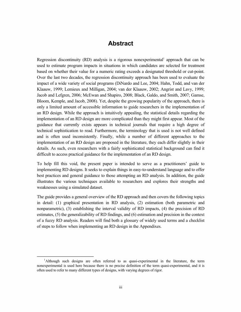
Abstract
Regression discontinuity (RD) analysis is a rigorous nonexperimental1 approach that can be used to estimate program impacts in situations in which candidates are selected for treatment based on whether their value for a numeric rating exceeds a designated threshold or cut-point. Over the last two decades, the regression discontinuity approach has been used to evaluate the impact of a wide variety of social programs (DiNardo and Lee, 2004; Hahn, Todd, and van der Klaauw, 1999; Lemieux and Milligan, 2004; van der Klaauw, 2002; Angrist and Lavy, 1999; Jacob and Lefgren, 2006; McEwan and Shapiro, 2008; Black, Galdo, and Smith, 2007; Gamse, Bloom, Kemple, and Jacob, 2008). Yet, despite the growing popularity of the approach, there is only a limited amount of accessible information to guide researchers in the implementation of an RD design. While the approach is intuitively appealing, the statistical details regarding the implementation of an RD design are more complicated than they might first appear. Most of the guidance that currently exists appears in technical journals that require a high degree of technical sophistication to read. Furthermore, the terminology that is used is not well defined and is often used inconsistently. Finally, while a number of different approaches to the implementation of an RD design are proposed in the literature, they each differ slightly in their details. As such, even researchers with a fairly sophisticated statistical background can find it difficult to access practical guidance for the implementation of an RD design.
To help fill this void, the present paper is intended to serve as a practitioners’ guide to implementing RD designs. It seeks to explain things in easy-to-understand language and to offer best practices and general guidance to those attempting an RD analysis. In addition, the guide illustrates the various techniques available to researchers and explores their strengths and weaknesses using a simulated dataset.
The guide provides a general overview of the RD approach and then covers the following topics in detail: (1) graphical presentation in RD analysis, (2) estimation (both parametric and nonparametric), (3) establishing the interval validity of RD impacts, (4) the precision of RD estimates, (5) the generalizability of RD findings, and (6) estimation and precision in the context of a fuzzy RD analysis. Readers will find both a glossary of widely used terms and a checklist of steps to follow when implementing an RD design in the Appendixes.
1Although such designs are often referred to as quasi-experimental in the literature, the term
nonexperimental is used here because there is no precise definition of the term quasi-experimental, and it is often used to refer to many different types of designs, with varying degrees of rigor.


v
Contents
Acknowledgments ii Abstract iii List of Exhibits vii 1 Introduction 1 2 Overview of the Regression Discontinuity Approach 4
3 Graphical Presentations in the Regression Discontinuity Approach 9
4 Estimation 18
5 Establishing the Internal Validity of Regression Discontinuity Impact
Estimates 41
6 Precision of Regression Discontinuity Estimates 50
7 Generalizability of Regression Discontinuity Findings 58
8 Sharp and Fuzzy Designs 61
9 Concluding Thoughts 71
Appendix A Glossary 74 B Checklists for Researchers 78 C For Further Investigation 83 References 87


vii
List of Exhibits
Table
1 Specification Test for Selecting Optimal Bin Width 16
2 Parametric Analysis for Simulated Data 27
3 Sensitivity Analyses Dropping Outermost 1%, 5%, and 10% of Data 28
4 Cross-Validation Criteria for Various Bandwidths 35
5 Estimation Results for Two Bandwidth Choices 36
6 Collinearity Coefficient and Sample Size Multiple for a Regression
Discontinuity Design Relative to an Otherwise Comparable Randomized
Trial, by the Distribution of Ratings and Sample Allocation
56
Figure
1 Two Ways to Characterize Regression Discontinuity Analysis 5
2 Scatter Plot of Rating (Pretest) vs. Outcome (Posttest) for Simulated Data 11
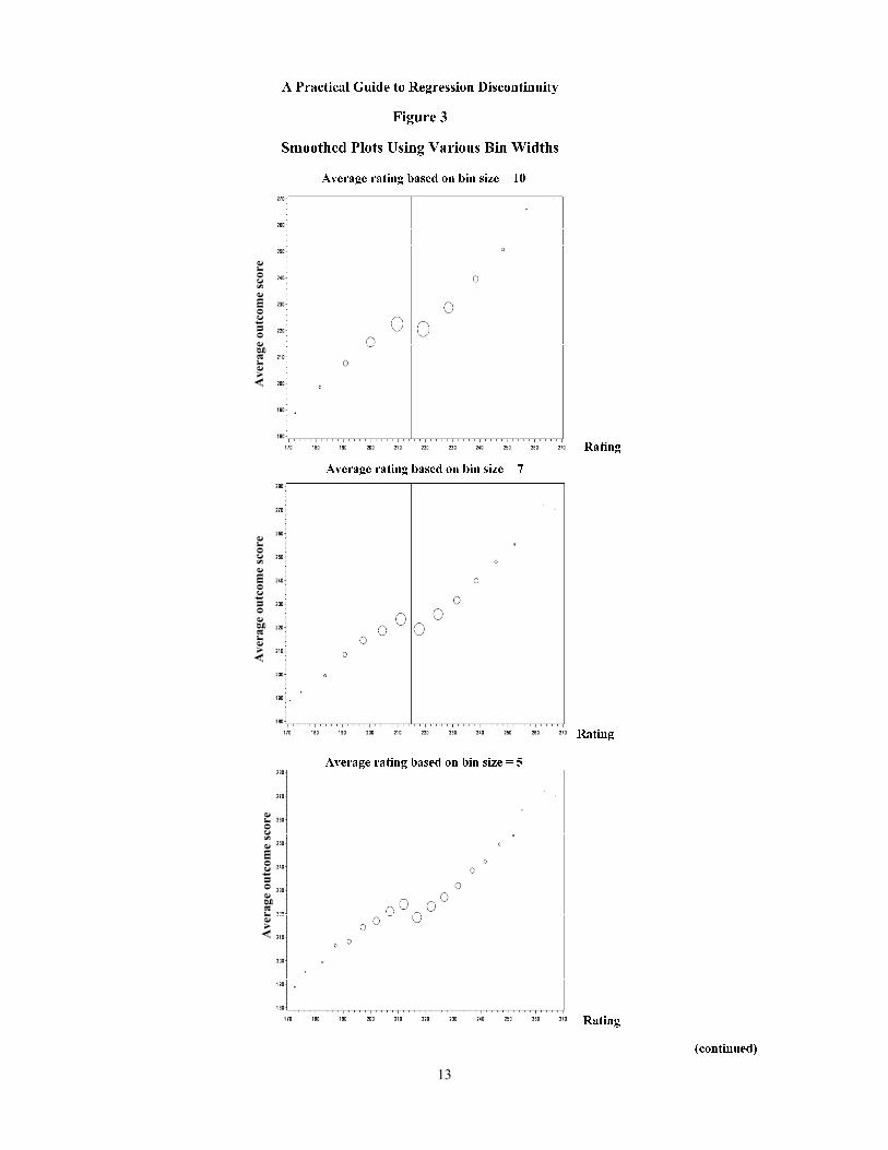
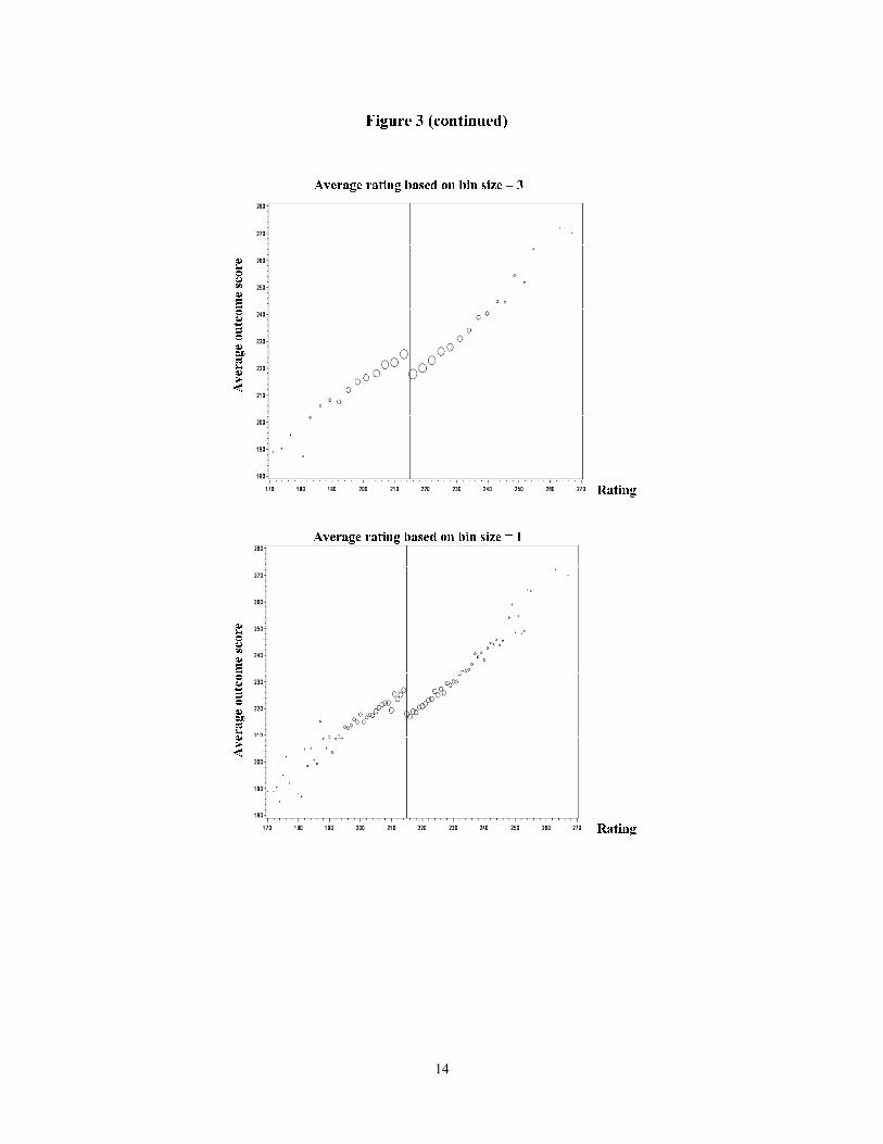
3 Smoothed Plots Using Various Bin Widths 13
4 Regression Discontinuity Estimation with an Incorrect Functional Form 19
5 Boundary Bias from Comparison of Means vs. Local Linear Regression
(Given Zero Treatment Effect)
30
6 Cross-Validation Procedure 32
7 Plot of Relationship between Bandwidth and RD Estimate, with 95%
Confidence Intervals
37
8 Plot of Rating vs. a Nonaffected Variable (Age) 45
9 Manipulation at the Cut-Point 46
10 Density of Rating Variable in Simulated Data Using a Bin Size of 3 48
11 Alternative Distributions of Rating 53
12 Distribution of Ratings in Simulated Data 55
13 How Imprecise Control Over Ratings Affects the Distribution of
Counterfactual Outcomes at the Cut-Point of a Regression Discontinuity
Design
59
14 The Probability of Receiving Treatment as a Function of the Rating 62
15 Illustrative Regression Discontinuity Analyses 64
16 The Probability of Receiving Treatment as a Function of the Rating in a
Fuzzy RD
69


1 Introduction
In recent years, an increased emphasis has been placed on the use of random assignment studies to evaluate educational interventions. Random assignment is considered the gold standard in empirical evaluation work, because when implemented properly, it provides unbiased estimates of program impacts and is easy to understand and interpret. The recent emphasis on random assignment studies by the U.S. Department of Education’s Institute for Education Sciences has resulted in a large number of high-quality random assignment studies. Spybrook (2007) identi-fied 55 randomized studies on a broad range of interventions that were under way at the time. Such studies provide rigorous estimates of program impacts and offer much useful information to the field of education as researchers and practitioners strive to improve the academic achievement of all children in the United States.
However, for a variety of reasons, it is not always practical or feasible to implement a random assignment study. Sometimes it can be difficult to convince individuals, schools, or dis-tricts to participate in a random assignment study. Participants often view random assignment as unfair or are reluctant to deny their neediest schools or students access to an intervention that could prove beneficial (Orr, 1998). In some instances, the program itself encourages participants to focus their resources on the students or schools with the greatest need. For example, the legis-lation for the Reading First program (part of the No Child Left Behind Act) stipulated that states and Local Education Agencies (LEAs) direct their resources to schools with the highest poverty and lowest levels of achievement. Other times, stakeholders want to avoid the possibility of competing estimates of program impacts. Finally, random assignment requires that participants be randomly assigned prior to the start of program implementation. For a variety of reasons, some evaluations must be conducted after implementation of the program has already begun, and, as such, methods other than random assignment must be employed.
For these reasons, it is imperative that the field of education continue to pursue and learn more about the methodological requirements of rigorous nonexperimental designs. Tom Cook has recently argued that a variety of nonexperimental methods can provide causal esti-mates that are comparable to those obtained from experiments (Cook, Shadish, and Wong, 2008). One such nonexperimental approach that has been of widespread interest in recent years is regression discontinuity (RD).
RD analysis applies to situations in which candidates are selected for treatment based on whether their value for a numeric rating (often called the rating variable) falls above or be-low a certain threshold or cut-point. For example, assignment to a treatment group might be de-termined by a school’s average achievement score on a statewide exam. Schools scoring below a certain threshold are selected for inclusion in the treatment group, and schools scoring above
1
the threshold constitute the comparison group. By properly controlling for the value of the rat-ing variable (which, in this case, is the average achievement score) in the regression equation, one can account for any unobserved differences between the treatment and comparison group.
RD was first introduced by Thistlethwaite and Campbell (1960) as an alternative meth-od for evaluating social programs. Their work generated a flurry of related activity, which sub-sequently died out. Economists revived the approach (Goldberger, 1972, 2008; van der Klaauw, 1997, 2002; Angrist and Lavy, 1999), formalized it (Hahn, Todd, and van der Klaauw, 2001), strengthened its estimation methods (Imbens and Kalyanaraman, 2009), and began to apply it to many different research questions. This renaissance culminated in a 2008 special issue on RD analysis in the Journal of Econometrics.
Over the last two decades, the RD approach has been used to evaluate, among other things, the impact of unionization (DiNardo and Lee, 2004), anti-discrimination laws (Hahn, Todd, and van der Klaauw, 1999), social assistance programs (Lemieux and Milligan, 2004), limits on unemployment insurance (Black, Galdo, and Smith, 2007), and the effect of financial aid offers on college enrollment (van der Klaauw, 2002). In primary and secondary education, it has been used to estimate the impact of class size reduction (Angrist and Lavy, 1999), remedial education (Jacob and Lefgren, 2006), delayed entry to kindergarten (McEwan and Shapiro, 2008), and the impact of the Reading First program on instructional practice and student achievement (Gamse, Bloom, Kemple, and Jacob, 2008).
However, despite the growing popularity of the RD approach, there is only a limited amount of accessible information to guide researchers in the implementation of an RD design. While the approach is intuitively appealing, the statistical details regarding the implementation of an RD design are more complicated than they might first appear. Most of the guidance that currently exists appears in technical journals that require a high degree of technical sophistica-tion to read. Furthermore, the terminology used is not well defined and is often used inconsist-ently. Finally, while a number of different approaches to the implementation of an RD design are proposed in the literature, they each differ slightly in their details. As such, even researchers with a fairly sophisticated statistical background find it difficult to find practical guidance for the implementation of an RD design.
To help fill this void, the present paper is intended to serve as a practitioner’s guide to implementing RD designs. It seeks to explain things in easy-to-understand language and to offer best practices and general guidance to those attempting an RD analysis. In addition, this guide illustrates the various techniques available to researchers and explores their strengths and weak-nesses using a simulated data set, which has not been done previously.
We begin by providing an overview of the RD approach. We then provide general rec-ommendations on presenting findings graphically for an RD analysis. Such graphical analyses
2

are a key component of any well-implemented RD approach. We then discuss the following in detail: (1) approaches to estimation, (2) how to assess the internal validity of the design, (3) how to assess the precision of an RD design, and (4) determining the generalizability of the findings. Throughout, we focus on the case of a “sharp” RD design. In the concluding section, we offer a short discussion of “fuzzy” RD designs and their estimation and precision.
Definition of Terms Many different technical terms are used in the context of describing, discussing, and implement-ing RD designs. We have found in our review of the literature that people sometimes use the same words to refer to different things or use different words to refer to the same thing. Throughout this document, we have tried to be consistent in our use of terminology. Further-more, every time we introduce a new term, we define it, and a definition of that term — along with other terms used to refer to the same thing — can be found in the glossary in Appendix A. Words that appear in the glossary are underlined in the text.
Checklist for Researchers In addition to the glossary, you will find in Appendix B a list of steps to following when im-plementing an RD design. There are two checklists: one for researchers conducting a retrospec-tive RD study and one for researchers who are planning a prospective RD study. Readers may find it helpful to print out the appropriate checklist and use it to follow along with the text of this document.
Researchers interested in conducting an RD design in the context of educational evalua-tion should also consult the What Works Clearinghouse guidelines on RD designs (http://ies.ed.gov/ncee/wwc/pdf/wwc_rd.pdf).
3
2 Overview of the Regression Discontinuity Approach1
In the context of an evaluation study, the RD design is characterized by a treatment assignment that is based on whether an applicant falls above or below a cut-point on a rating variable, gen-erating a discontinuity in the probability of treatment receipt at that point. The rating variable may be any continuous variable measured before treatment, such as a pretest on the outcome variable or a rating of the quality of an application. It may be determined objectively or subjec-tively or in both ways. For example, students might need to meet a minimum score on an objec-tive assessment of cognitive ability to be eligible for a college scholarship. Students who score above the minimum will receive the scholarship, and those who score below the minimum will not receive the scholarship.
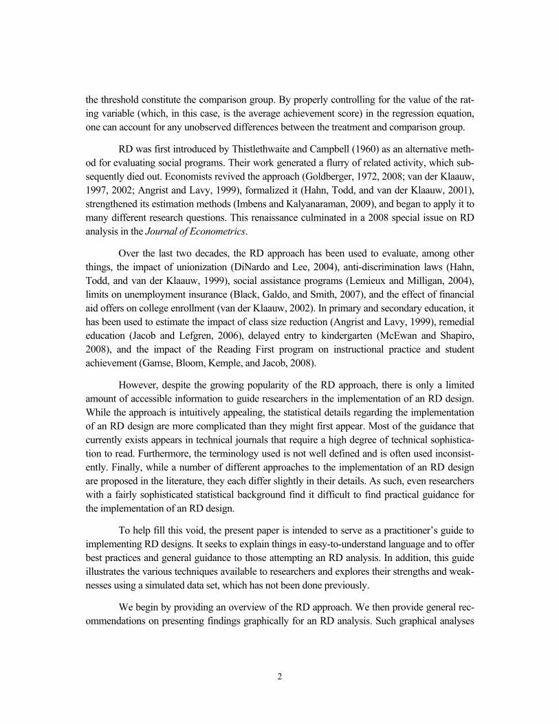
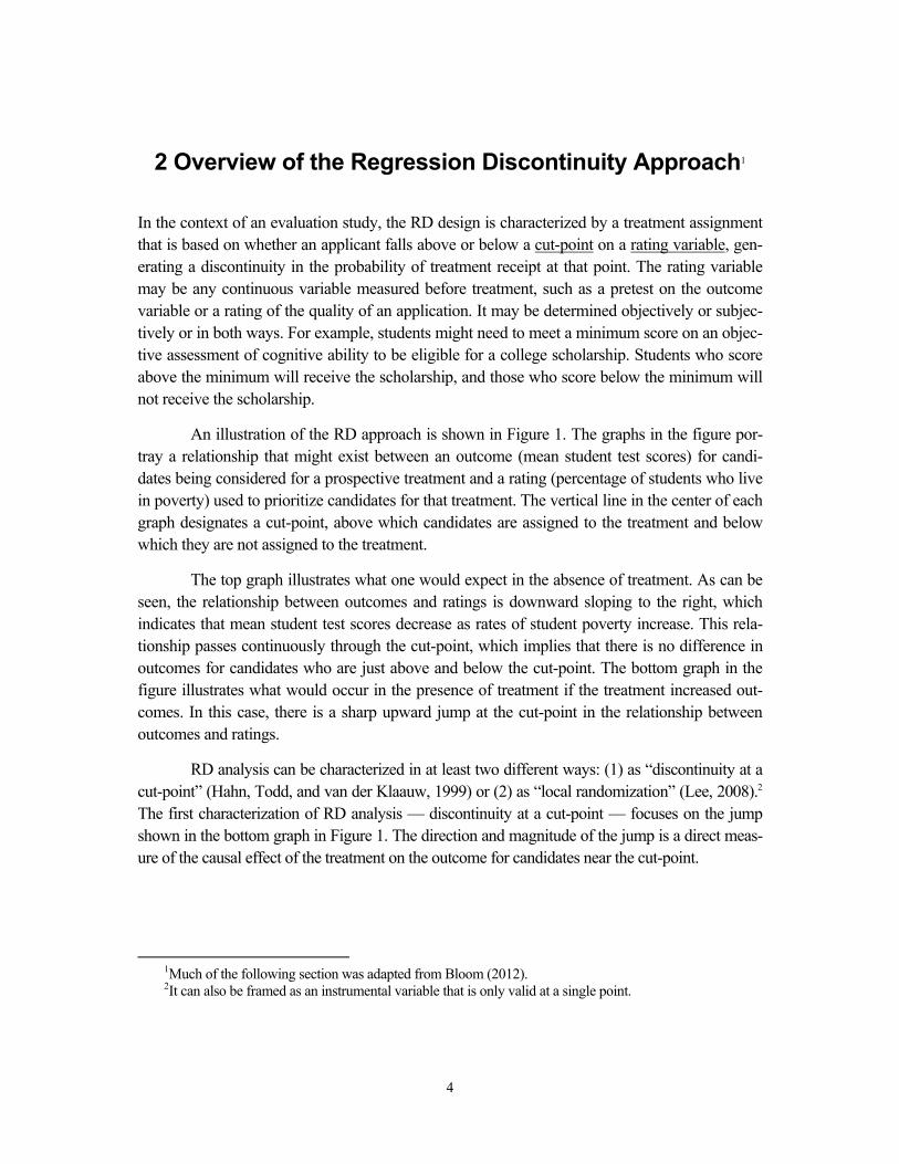
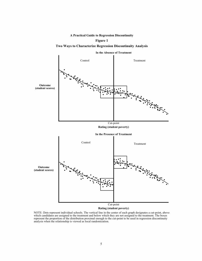
An illustration of the RD approach is shown in Figure 1. The graphs in the figure por-tray a relationship that might exist between an outcome (mean student test scores) for candi-dates being considered for a prospective treatment and a rating (percentage of students who live in poverty) used to prioritize candidates for that treatment. The vertical line in the center of each graph designates a cut-point, above which candidates are assigned to the treatment and below which they are not assigned to the treatment.
The top graph illustrates what one would expect in the absence of treatment. As can be seen, the relationship between outcomes and ratings is downward sloping to the right, which indicates that mean student test scores decrease as rates of student poverty increase. This rela-tionship passes continuously through the cut-point, which implies that there is no difference in outcomes for candidates who are just above and below the cut-point. The bottom graph in the figure illustrates what would occur in the presence of treatment if the treatment increased out-comes. In this case, there is a sharp upward jump at the cut-point in the relationship between outcomes and ratings.
RD analysis can be characterized in at least two different ways: (1) as “discontinuity at a cut-point” (Hahn, Todd, and van der Klaauw, 1999) or (2) as “local randomization” (Lee, 2008).2 The first characterization of RD analysis — discontinuity at a cut-point — focuses on the jump shown in the bottom graph in Figure 1. The direction and magnitude of the jump is a direct meas-ure of the causal effect of the treatment on the outcome for candidates near the cut-point.
1Much of the following section was adapted from Bloom (2012). 2It can also be framed as an instrumental variable that is only valid at a single point.
4
Outcome(student scores)
Rating (student poverty)
Control Treatment
TreatmentControl
In the Presence of Treatment
In the Absence of Treatment
A Practical Guide to Regression DiscontinuityFigure 1
Two Ways to Characterize Regression Discontinuity Analysis
Outcome(student scores)
Rating (student poverty)NOTE: Dots represent individual schools. The vertical line in the center of each graph designates a cut-point, above which candidates are assigned to the treatment and below which they are not assigned to the treatment. The boxes represent the proportion of the distribution proximal enough to the cut-point to be used in regression discontinuity analysis when the relationship is viewed as local randomization.
Cut-point
Cut-point
5
The second characterization of RD analysis — local randomization — is based on the premise that differences between candidates who just miss and just make a threshold are ran-dom. This could occur, for example, from random error in test scores used to rate candidates. Candidates who just miss the cut-point are thus, on average, identical to those who just make it, except for exposure to treatment. Any difference in subsequent mean outcomes must therefore be caused by treatment. In this case, one can simply compare the mean outcomes for schools just to the left and just to the right of the cut-point (as represented by the two boxes in Figure 1).
Fuzzy versus Sharp RD Designs In addition to these two characterizations, the existing literature typically distinguishes two types of RD designs: the sharp design, in which all subjects receive their assigned treatment or control condition, and the fuzzy design, in which some subjects do not. The “fuzzy” design is analogous to having no-shows (treatment group members who do not receive the treatment) and/or crossovers (control group members who do receive the treatment) in a randomized ex-periment. Throughout this document, we focus on the case of a sharp design. In the concluding section, we return to the case of fuzzy designs and discuss their properties in more detail.
Conditions for Internal Validity The RD approach is appealing from a variety of perspectives. Situations that lend themselves to an RD approach occur frequently in practice, and one can often obtain existing data and use it post hoc to conduct analyses of program impact — at significantly lower cost than conducting a random assignment study. Even in prospective studies, the RD approach can avoid many of the pitfalls of a random assignment design, since it works with the selection process that is already in place for program participation rather than requiring a random selection of participants.3 However, because it is a nonexperimental approach, it must meet a variety of conditions to pro-vide unbiased impact estimates and to approach the rigor of a randomized experiment (for ex-ample, Hahn, Todd, and van der Klaauw, 2001; Shadish, Cook, and Campbell, 2002). Specifi-cally:
• The rating variable cannot be caused by or influenced by the treatment. In other words, the rating variable is measured prior to the start of treat-ment or is a variable that can never change.
3In practice, a researcher conducting a prospective study may have to convince participants to use a rating-
based assignment process.
6

• The cut-point is determined independently of the rating variable (that is, it is exogenous), and assignment to treatment is entirely based on the candidate ratings and the cut-point. For example, when selecting students for a scholarship, the selection committee cannot look at which students received high scores and set the cut-point to ensure that certain students are included in the scholarship pool, nor can they give scholarships to students who did not meet the threshold.
• Nothing other than treatment status is discontinuous in the analysis inter-val (that is, there are no other relevant ways in which observations on one side of the cut-point are treated differently from those on the other side). For example, if schools are assigned to treatment based on test scores, but the cut-point for receiving the treatment is the same cut-point used for determining which schools are placed on an academic warning list, then the schools who receive the treatment will also receive a whole host of other interventions as a result of their designation as a school on academic warning. Thus, the RD design would be valid for distinguish-ing the impacts of the combined effect of the treatment and academic warning status, but not for isolating the impact of the treatment of inter-est. Similarly, a discontinuity would occur if there were some type of manipulation regarding which individuals or groups received the treat-ment.
• The functional form representing the relationship between the rating var-iable and the outcome, which is included in the estimation model and can be represented by ( ), is continuous throughout the analysis interval absent the treatment and is specified correctly.4
With these conditions in mind, this document outlines the key issues that researchers must consider when designing and implementing an RD approach. These key issues all relate to ensuring that the set of conditions listed above are met.
Throughout the paper, we use a simulated data set, based on actual data, to explore each of these issues in more detail and offer some practical advice to researchers about how to ap-proach the design and analysis of an RD study. The simulated data set is constructed using actu-al student test scores on a seventh-grade math assessment. From the full data set, we selected
4This last condition applies only to parametric estimators. If there are other discontinuities in the analysis
interval, the analyst will need to restrict the range of the data so that it includes only the discontinuity that iden-tifies the impact of interest.
7

two waves of student test scores and used those two test scores as the basis for the simulated data set. One test score (the pretest) was used as the rating variable and the other (the posttest) was used as the outcome. The pretest mean was 215, with a standard deviation of 12.9, and the posttest mean was 218, with a standard deviation of 14.7. The test scores are from a computer adaptive test focusing on certain math skills. Only observations with both pre- and posttest scores were included. We picked the median of the pretest (= 215) as the cut-point (so that we would have a balanced ratio between the treatment and control units) and added a treatment ef-fect of 10 scale score points to the posttest score of everyone whose pretest score fell below the median.5 From the original data set, we were able to obtain student characteristics, such as race/ethnicity, age, gender, special education status, English as a Second Language (ESL) sta-tus, and free/reduced lunch status, and include them in the simulated data set.
5In our examples, we focus on the case of homogeneous treatment effects for ease of interpretation and
simplicity.
8
3 Graphical Presentations in the Regression Discontinuity Approach
We begin our discussion by explaining graphical presentations in the context of an RD design and the procedure used to generate them. Graphical presentations provide a simple yet powerful way to visualize the identification strategy of the RD design and hence should be an integral part of any RD analysis. We begin with a discussion of graphical presentations, because (1) they should be the first step in any RD analyses, (2) they provide an intuitive way to conceptualize the RD approach, and (3) the techniques used for graphical analyses lay the groundwork for our discussion of estimation in section 4.
In this section, we provide information on how to create graphical tools that can be used in all aspects of planning and implementing an RD design. As an example, we will explain how to create a graph that plots the relationship between the outcome of interest and the rating varia-ble and will use our simulated data to illustrate. The same procedures can also be used to create other types of graphs. Typically, there are four types of graphs that are used in RD analyses, each of which explores the relationship between the rating variable and other variables of inter-est: (1) A graph plotting the probability of receiving treatment as a function of the rating varia-ble (to visualize the degree of treatment contrast and to determine whether the design is “sharp” or “fuzzy”); (2) graphs plotting the relationship between nonoutcome variables and the rating variable (to help assess the internal validity of the design); (3) a graph of the density of the rat-ing variable (also to assess the internal validity of the design by assessing whether there was any manipulation of ratings around the cut-point); and (4) a graph plotting the relationship between the outcome and the rating variable (to help visualize the size of the impact and explore the functional form of the relationship between outcomes and ratings). We will discuss each of these graphs and their purposes in more detail in later sections.
Basic Approach All RD analysis should begin with a graphical presentation in which the value of the outcome for each data point is plotted on the vertical axis, and the corresponding value of the rating is plotted on the horizontal axis. First, the graphical presentation provides a powerful visual an-swer to the question of whether or not there is evidence of a discontinuity (or “jump”) in the outcome at the cut-off point. The formal statistical methods discussed in later parts of this paper are just more sophisticated versions of getting at this jump, and if this basic graphical approach does not show evidence of a discontinuity, there is little chance of finding any statistically ro-bust and significant treatment effects using more complicated statistical methods.
9
Second, the graph provides a simple way of visualizing the relationship between the outcome and the rating variable. Seeing what this relationship looks like can provide useful guidance in choosing the functional form for the regression models used to formally estimate the treatment effect.
Third, the graph also allows one to check whether there is evidence of jumps at points other than the cut-off. If the graph visually shows such evidence, it implies that there might be factors other than the treatment intervention that are affecting the relationship between the out-come and the rating variable and, therefore, calls into question the interpretation of the disconti-nuity observed at the cut-off point, that is, whether or not this jump can be solely attributed to the treatment of interest.6
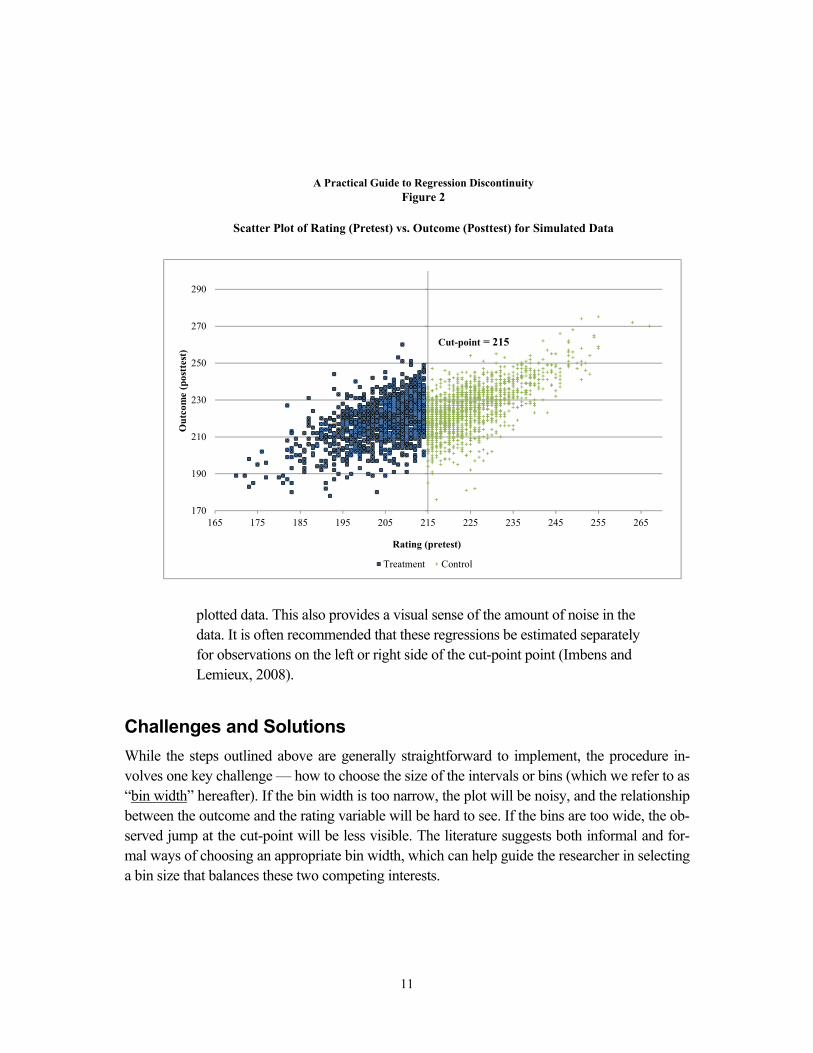
The graph in Figure 2 illustrates such a plot for an upward-sloping outcome (posttest) and rating (pretest) relationship that has a downward shift (discontinuity) in outcomes at the cut-point. However, as is typical, the plot of individual data points is quite noisy, and the individual data points in the graph bounce around quite a bit, making it difficult to determine whether or not there is, in fact, a discontinuity at the cut-point or at any other point along the distribution. To effectively summarize the pattern in the data without losing important information, the lit-erature suggests presenting a “smoothed” plot of the outcome on the rating variable. One can take the following steps to create such a graph:
1. Divide the rating variable into a number of equal-sized intervals, which are often referred to as “bins.” Start defining the bins at the cut-point and work your way out to the right and left to make sure that no bin “straddles” the cut-point (that is, no bin contains both treatment and control observations).
2. Calculate the average value of the outcome variable and the midpoint value of the rating variable for each bin and count the number of observations in each bin.
3. Plot the average outcome values for each bin on the Y-axis against the mid-point rating values for each bin on the X-axis, using the number of observa-tions in each bin as the weight, so that the size of a plotted dot reflects the number of observations contained in that data point.
4. To help readers better visualize whatever patterns exit in the data, one can superimpose flexible regression lines (such as lowess lines7) on top of the
6This discussion is drawn from Lee and Lemieux (2010). 7A lowess line is a smoothing plot of the relationship between the outcome and rating variables based on
locally weighted regression. It can be obtained using the -lowess- command in STATA.
10
plotted data. This also provides a visual sense of the amount of noise in the data. It is often recommended that these regressions be estimated separately for observations on the left or right side of the cut-point point (Imbens and Lemieux, 2008).
Challenges and Solutions While the steps outlined above are generally straightforward to implement, the procedure in-volves one key challenge — how to choose the size of the intervals or bins (which we refer to as “bin width” hereafter). If the bin width is too narrow, the plot will be noisy, and the relationship between the outcome and the rating variable will be hard to see. If the bins are too wide, the ob-served jump at the cut-point will be less visible. The literature suggests both informal and for-mal ways of choosing an appropriate bin width, which can help guide the researcher in selecting a bin size that balances these two competing interests.
A Practical Guide to Regression DiscontinuityFigure 2
Scatter Plot of Rating (Pretest) vs. Outcome (Posttest) for Simulated Data
170
190
210
230
250
270
290
165 175 185 195 205 215 225 235 245 255 265
Out
com
e (p
ostt
est)
Rating (pretest)
Treatment Control
Cut-point = 215
11
Informal Tests
Informally, researchers can try several different bin widths and visually compare them to assess which bin width makes the graph most informative. Ideally, one wants a bin width that is narrow enough so that existing patterns in the data are visible, especially around the cut-point, but that is also wide enough so that noise in the data does not overpower its signal.
The plots in Figure 3 use our simulated data to show graphs of the outcome plotted against the rating for bin widths of 10, 7, 5, 3, and 1 units of the rating variable (the pretest in the present example). In our simulated data set, we know that there is an impact of 10 points, so in our example, we should see a clear jump at the cut-point. If we don’t, then the bins are too wide. Comparing these plots, it is clear that bin widths of 10 or 7 (the first and second plots) are probably too wide, because it is difficult to determine whether or not there is a jump at the cut-point. On the other hand, bin widths of 1 or 2 (first and second-to-last plots) are probably too narrow, because the plotted dots toward the tails of the plot are too scattered to show any clear relationship between the outcome and the rating variable. Therefore, one is left with a choice of bin width of 3 or 5. Based on the plots, it is very hard to see which of these two bin widths is preferable. This is when some formal guidance in the selection process might be useful.
Formal Tests
Two types of formal tests have been suggested to facilitate the selection of a bin width. Both tests focus on whether the proposed bin width is too wide. When using these tests, there-fore, one would continue to make the bin width wider until it was deemed to be too wide. The first is an F-test based on the idea that if a bin width is too wide, using narrower bins would provide a better fit to the data. The test involves the following steps:
1. For a given bin width h, create K dichotomous indicators, one for each bin.
2. Regress the outcome variable on this set of K indicators (call this regression 1).
3. Divide each bin into two equal-sized smaller bins by increasing the number of bins to 2K and reducing the bin width from h to h/2.
4. Create 2K indicators, one for each of the smaller bins.
5. Regress the outcome variable on the new set of 2K indicators (regression 2).
6. Obtain R-squared values from both regressions: from regression 1 and from regression 2.
12
Ave
rage
out
com
e sc
ore
Ave
rage
out
com
e sc
ore
Ave
rage
out
com
e sc
ore
13
14

7. Calculate an F statistic using the following formula:8 = ( − )/(1 − )/( − − 1) Where n is the total number of observations in the regression. A p-value cor-responding to this F statistic can be obtained using the degrees of freedom K and n-K-1. This tests whether the “extra” bin indicators improve the predic-tive power of the regression by an amount that is statistically significant.
8. If the resulting F statistic is not statistically significant, the bin width of h is not oversmoothing the data, because further dividing the bins does not signif-icantly increase the explanatory power of the bin indicators.
9. The researcher can test various bin widths in this way to find the largest bin width that does not “oversmooth” the data, using the visual plots to help nar-row the number of tests. In our simulated data, we would likely test the bin width of 3 and 5 based on a visual inspection of the plots.
The second proposed test, also an F-test, is based on the idea that a bin width is too wide if there is still a systematic relationship between the outcome and rating within each bin. If such a relationship exists, then the average value of the outcome within the bin is not repre-sentative of the outcome value at the boundaries of the bin, which is what one cares about in an RD analysis. To implement this test, the researcher can take the following steps:
1. For a given bin width h, create K dichotomous indicators, one for each bin.
2. Regress the outcome on the set of K indicator variables (regression 1).
3. Create a set of interaction terms between the rating variable and each of the K indicator variables.
4. Interact these K indicator variables with the rating variable and regress the outcome on the set of bin indicators as well as on the set of interaction terms created in step 3.
5. Construct an F-test to see if the interaction terms are jointly significant.9 If they are, then the tested bin width is too large.
8Any standard statistical software package can produce this test result automatically. 9The degrees of freedom for this F test are K and n-K-1 (n is the number of observations).
15
16
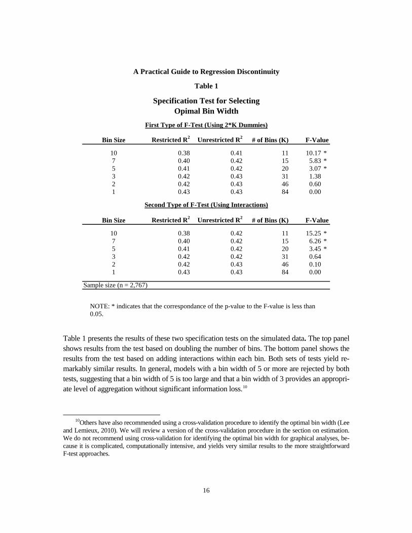
Table 1 presents the results of these two specification tests on the simulated data. The top panel shows results from the test based on doubling the number of bins. The bottom panel shows the results from the test based on adding interactions within each bin. Both sets of tests yield re-markably similar results. In general, models with a bin width of 5 or more are rejected by both tests, suggesting that a bin width of 5 is too large and that a bin width of 3 provides an appropri-ate level of aggregation without significant information loss.10
10Others have also recommended using a cross-validation procedure to identify the optimal bin width (Lee
and Lemieux, 2010). We will review a version of the cross-validation procedure in the section on estimation. We do not recommend using cross-validation for identifying the optimal bin width for graphical analyses, be-cause it is complicated, computationally intensive, and yields very similar results to the more straightforward F-test approaches.
Restricted R2 Unrestricted R2 # of Bins (K)
0.38 0.41 11 10.17 *0.40 0.42 15 5.83 *0.41 0.42 20 3.07 *0.42 0.43 31 1.380.42 0.43 46 0.600.43 0.43 84 0.00
Restricted R2 Unrestricted R2 # of Bins (K)
0.38 0.42 11 15.25 *0.40 0.42 15 6.26 *0.41 0.42 20 3.45 *0.42 0.42 31 0.640.42 0.43 46 0.100.43 0.43 84 0.00
A Practical Guide to Regression Discontinuity
Table 1
Specification Test for SelectingOpimal Bin Width
First Type of F-Test (Using 2*K Dummies)
Bin Size F-Value
1075321
Second Type of F-Test (Using Interactions)
Bin Size F-Value
1075321
Sample size (n = 2,767)
NOTE: * indicates that the correspondance of the p-value to the F-value is less than 0.05.
Recommendations As mentioned before, the main purpose of the graphical analysis in an RD design is to provide a simple way to visualize the relationship between an outcome variable and a rating variable as well as to indicate the magnitude of the discontinuity at the cut-point. For these purposes, we recommend that researchers follow three steps in selecting a bin width for a graphical RD presentation:
1. Plot the data using a range of bin widths. Visually inspect the plots and rule out the ones that are clearly too wide or too narrow to visualize the relation-ship between outcome and rating.
2. Using the remaining bin widths, conduct the two F tests specified to identify bin widths that oversmooth the data.
3. Among the remaining choices, pick the widest bin width that is not rejected by either one of the F-tests.
Using the recommended procedure, we select a bin width of 3 for the graphical analysis of our example. As can be seen in Figure 3, this plot indicates a rather linear relationship be-tween the posttest score and the pretest score for the large part of the data range around the cut-point, while data points toward the far ends of data range show some signs of curvature.
So far, our discussion has focused on the graph of the outcome variable and the rating variable. The same procedures can be used to create other graphical representations of the data. As discussed at the beginning of this section, these measures include graphs that depict the probability of receiving treatment, plots of baseline or nonoutcome variables against the rating, and plots that show the density for the rating variable (all of which also involve selecting a bin width for the rating variable). These graphs are discussed in more detail in later sections.
One question that arises when creating these other graphs is whether to select a different bin width for each graph (to maximize the visual power of the graph) or to keep the bin width the same across all graphs in order to enable comparisons across the graphs. Either choice in-volves trade-offs, but we recommend keeping the bin size the same for all graphical displays in order to facilitate comparisons, unless doing so would severely compromise the visual power of the graph.
17
4 Estimation
Next, we turn to the task of estimating treatment effects using an RD design. A major problem with any nonexperimental approach is the threat of selection bias. If the selection process could be completely known and perfectly measured, then one could adjust for differences in selection to obtain an unbiased estimate of treatment effect. The same is true of a RD design. While the conditions of an RD design promise complete knowledge of the rating variable, the design itself does not guarantee full knowledge of the functional form that this variable should take in the impact model. The challenge is to identify the correct functional form of the relationship be-tween the rating variable and the outcome measure in the absence of treatment.
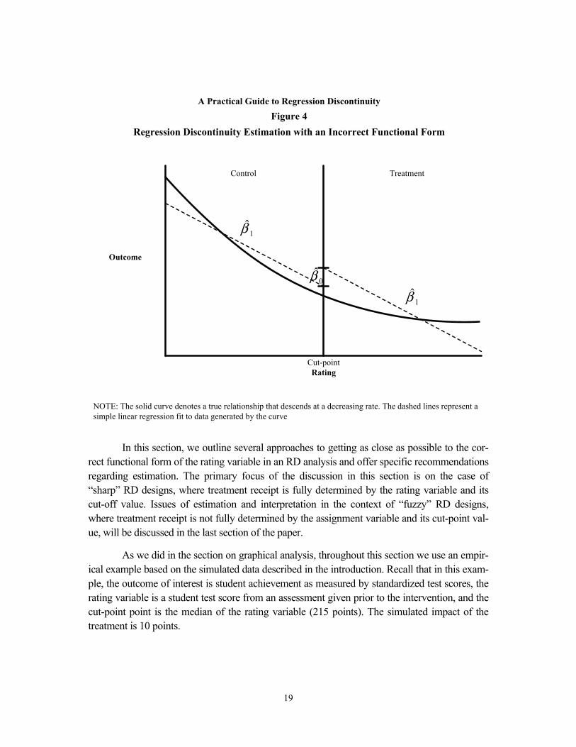
To the extent that the specified functional form is correct, the estimator implied by the RD model will be an unbiased estimator of the mean program impact at the cut-point. If the functional form is incorrectly specified, treatment effects will be estimated with bias. For exam-ple, if the true functional form is highly nonlinear, a simple linear model can produce mislead-ing results. Figure 4 illustrates this situation. The solid curve in the figure denotes a true rela-tionship that descends at a decreasing rate and passes continuously through the cut-point with no effect from the treatment. Dashed lines in the figure represent a simple linear regression fit to data generated by the true curve. Imposing a constant slope ( ) for the treatment group and control group understates the average magnitude of the control-group slope and overstates the average magnitude of the treatment-group slope. This creates an apparent shift at the cut-point, which gives the mistaken impression of a discontinuity in the true function and implies that there is an impact of the program, when in fact there is none.
There are two theoretical reasons for a nonlinear relationship between outcomes and ratings. One is that the relationship between mean counterfactual outcomes and ratings is non-linear, perhaps because of a ceiling effect or a floor effect; the other is that treatment effects vary systematically with ratings. For example, candidates with the highest ratings might experi-ence the largest (or smallest) treatment effects. However, because RD analyses are seldom, if ever, guided by theory that is powerful enough to accurately predict such nuances, choosing a functional form is typically an empirical task.
As a result, methodologists suggest testing a variety of functional forms — including linear models, linear models with a treatment interaction, quadratic models, and quadratic mod-els with treatment interactions — as well as employing nonparametric estimation techniques such as local linear regression to make sure the functional form that is specified is as close as possible to the correct functional form. Much of the current literature discusses how to choose among these various specifications. For a review, see van der Klaauw (2008) and Cook (2008).
18
In this section, we outline several approaches to getting as close as possible to the cor-rect functional form of the rating variable in an RD analysis and offer specific recommendations regarding estimation. The primary focus of the discussion in this section is on the case of “sharp” RD designs, where treatment receipt is fully determined by the rating variable and its cut-off value. Issues of estimation and interpretation in the context of “fuzzy” RD designs, where treatment receipt is not fully determined by the assignment variable and its cut-point val-ue, will be discussed in the last section of the paper.
As we did in the section on graphical analysis, throughout this section we use an empir-ical example based on the simulated data described in the introduction. Recall that in this exam-ple, the outcome of interest is student achievement as measured by standardized test scores, the rating variable is a student test score from an assessment given prior to the intervention, and the cut-point point is the median of the rating variable (215 points). The simulated impact of the treatment is 10 points.
Outcome
Cut-pointRating
1β̂
1β̂0β̂
Control Treatment
A Practical Guide to Regression DiscontinuityFigure 4
Regression Discontinuity Estimation with an Incorrect Functional Form
NOTE: The solid curve denotes a true relationship that descends at a decreasing rate. The dashed lines represent a simple linear regression fit to data generated by the curve
19
Choosing the Most Appropriate Model Specification As described above, any RD analysis should begin with a visual examination of a plot of the outcome variable against the rating variable. Graphical analysis provides visual guidance for modeling the relationship between the rating variable and the outcome variable. For example, it may suggest that the relationship between the rating and outcome variable is nonlinear. To es-timate the exact magnitude of the discontinuity in outcomes at the cut-off point (the treatment effect) and to assess its statistical properties, one uses regression analyses.
Broadly speaking, there are two types of strategies for correctly specifying the function-al form in a single-rating RD case (Bloom, 2012). These correspond to the two characterizations of the RD described earlier — “discontinuity at the cut-point” and “local randomization”:
• Parametric/global strategy: This strategy uses every observation in the sample to model the outcome as a function of the rating variable and treatment status. This method “borrows strength” from observations far from the cut-point score to estimate the average outcome for observa-tions near the cut-point score. To minimize bias, different functional forms for the rating variable — including the simplest linear form, quad-ratic, cubic, as well as its interactions with treatment — are tested by conducting F-tests on higher-order interaction terms and inspecting the residuals. This approach conceptualizes the estimation of treatment ef-fects as a “discontinuity at the cut-point.”
• Nonparametric/local strategy: In the simplest terms, this strategy views the estimation of treatment effects as local randomization and limits the analysis to observations that lie within the close vicinity of the cut-point (sometimes called a bandwidth), where the functional form is more likely to be close to linear. The main challenge here is selecting the right band-width. The bandwidth can be chosen visually by examining the distribu-tion of the rating variable or by seeking to minimize a clearly defined cross-validation criterion.11 Once the bandwidth is selected, a linear re-gression is estimated, using observations within one bandwidth on either side of the threshold (though polynomials of the rating variables can also be specified). This approach, which is one of many possible nonparamet-ric approaches, is often called local linear regression (or “local polyno-mial regression,” if polynomials are used in the estimation).
11For more details on the selection of the cross-validation criterion, see Imbens and Lemieux (2008). See
also Imbens and Kalyanaraman (2009) for an optimal, data-dependent rule for selecting the bandwidth.
20

One way to think about these two approaches is as follows: The parametric approach tries to pick the right model to fit a given data set, while the nonparametric approach tries to pick the right data set to fit a given model. Specifically, the parametric approach focuses on finding the optimal functional form between the outcome and the rating variable to fit the full set of data. At the same time, the most commonly used nonparametric regression analysis for RDDs — local linear regression — searches for the optimal data range within which a simple linear regression can produce a consistent estimate.
When choosing between these two strategies, one needs to consider the trade-off be-tween bias and precision. Since the parametric/global approach uses all available data in the estimation of treatment effects, it can potentially offer greater precision than the nonparametric, local approach.12 The trade-off is that it is often difficult to ensure that the functional form of the relationship between the conditional mean of the outcome and the rating variable is specified correctly over such a large range of data, and thus the potential for bias is increased. The non-parametric/local strategy substantially reduces the chances that bias will be introduced by using a much smaller portion of the data, but in most cases will have more limited statistical power due to the smaller sample size used in the analyses. This section uses the simulated data set to illustrate the key challenges facing each of these strategies and then discusses the pros and cons of these two approaches.
The Parametric/Global Strategy As already noted, the conventional “parametric” approach uses all available observations to es-timate treatment effects based on a specific functional form for the outcome/rating relationship. The following equation provides a simple way to make this estimation procedure operational:
where: = the average value of the outcome for those in the treatment group after controlling for the rating variable;
= the outcome measure for observation i; = 1 if observation i is assigned to the treatment group and 0 otherwise; = the rating variable for observation i, centered at the cut-point;
12We say potentially, since in some instances a higher-order functional form could actually reduce preci-
sion.
iiii rfTY εβα +++= )(0
iY
iT
ir
21

= a random error term for observation i, which is assumed to be inde-pendently and identically distributed.
The coefficient, for treatment assignment represents the marginal impact of the pro-
gram at the cut-point.
The rating variable is included in the impact model to correct for selection bias due to the selection on observables ( in this context) (Heckman and Robb, 1985). Many analysts will center the rating variable on the cut-point by creating a new variable ricut-score= (ri — cut-score) and then using ricut-score in the model. This helps with the interpretation of results by locating the intercept of the regression at the cut-point (since the value of the rating at the cut-point will now be zero) and allowing any shift at the cut-point to be interpreted as a shift in the intercept. To improve precision, covariates can also be added to the model, but they are not required for ob-taining unbiased or consistent estimates.
The function ( ) represents the relationship between the rating variable and the out-come. A variety of functional forms can be tested to determine which fits the data best, so that bias will be minimized. For example, the following models are often tested in the parametric analysis of the RD design:
1. linear = + ∙ + ∙ + 2. linear interaction = + ∙ + ∙ + ∙ ∙ + 3. quadratic = + ∙ + ∙ + ∙ + 4. quadratic interaction = + ∙ + ∙ + ∙ + ∙ ∙ + ∙∙ + 5. cubic = + ∙ + ∙ + ∙ + ∙ + 6. cubic interaction = + ∙ + ∙ + ∙ + ∙ + ∙ ∙+ ∙ ∙ + ∙ ∙ +
where the rating is centered at the cut-point and all variables are defined as before.
The first, third, and fifth models constrain the slope of the outcome/rating relationship to be identical on both sides of the cut-point, while the other three (two, four, and six) specify a different polynomial function of rating on either side of the cut-point. Including an interaction between the rating variable and the treatment can account for the fact that the treatment may impact not only the intercept, but also the slope of the regression line. This can be particularly important in situations where data that are very far from the cut-point are included in the analy-sis or in which there is nonlinearity in the relationship between the outcome and the rating. At the same time, increasing the complexity of the model — by allowing the slope to vary on ei-ther side of the cut-point — also reduces the power of the analysis (this is discussed in greater
iε
0β
ir
22

detail below). This may not matter much in an analysis that involves many observations, but it can be a limiting factor in smaller data sets. Therefore, we recommend using the simplest possi-ble model that can be justified based on the specification tests (described below).
Challenges and Solutions Selecting among the various functional forms is one of the greatest challenges for the paramet-ric approach to estimation. Several strategies have been proposed in the literature as ways to select the most appropriate functional form(s). Our preferred approach is one suggested by Lee and Lemieux (2010).
F-Test Approach
Lee and Lemieux (2010) suggest testing the set of candidate models (models 1-6 above) against the data that underlie the initial plot of the rating versus the outcomes, to see how well the model fits the data that are depicted in the graph.13
To implement this test, one can complete the following steps:
1. Create a set of indicator variables for K-2 of the bins used to graphically de-pict the data. Exclude any two of the bins to avoid having a model that is col-linear.
2. Run a regression (Regression 1) using the model you are trying to assess (one of the six models outlined above).
3. Run a second regression (Regression 2), which is identical to Regression 1, but also includes the bin indicator variables created in step 1.
4. Obtain R-squared values from each of the two regressions: fromregression2, and from regression 1.
5. Calculate an F statistic using the following formula:
= ( − )/(1 − )/( − − 1)
where n is the total number of observations in the regression, and K is the number of bin indicators included in the model.
13For detailed description of this approach, see Lee and Lemieux (2010).
23
6. A p-value corresponding to this F statistic can be obtained using the degrees of freedom K and n-K-1. If the resulting F statistic is not statistically signifi-cant, the data from each of the bins are not adding any additional information to the model. This indicates that the model being tested is not underspecified and therefore is not oversmoothing the data.14
Usually, one would start with a simple linear model. If the F-test for the linear model versus a model with the bin indicators 15 is not statistically significant, it implies that the sim-plest functional form adequately depicts the relationship between the outcome and the rating variables and therefore can serve as an appropriate choice for the RD estimation model. If, however, the F-test indicates oversmoothing of the data, a higher-order term (and its interaction with treatment indicator) needs to be added to the functional form and a new F-test carried out on this higher-order polynomial model. The idea is to keep adding higher-order terms to the polynomial until the F-test is no longer statistically significant.
It should be noted that the F-test approach is testing whether or not there is unexplained variability in the relationship between the outcome and rating that the specified model isn’t cap-turing; in other words, is something missing from the model? This is a more general approach than testing the statistical significance of individual terms in the model — for example, running a simple linear model and then adding an interaction term and testing whether or not the interac-tion is statistically significant. A more general approach is preferred under these circumstances, because it provides a higher level of confidence that the model has been specified correctly by indicating whether or not anything is missing, not whether or not a specific term adds to the ex-planatory power of the model.
AIC Approach
Another strategy that can be used is the Akaike information criterion (AIC) procedure. The AIC captures the bias-precision trade-off of using a more complex model. It is a measure of the relative goodness of fit of a statistical model. Conceptually, it describes the trade-off be-tween bias and variance in the model. Computationally, this measure increases with both the estimated residual variance as well as with the number of parameters (essentially the order of the polynomial) in the regression model. These two terms move in opposite directions as the model becomes more complex: The estimated residual variance should decrease with more
14Any standard statistical software package can produce this test result automatically. 15Note that we are talking about an F-test that compares the simple model versus the model that includes
the bin indicators and not the F-test that is generated automatically by most regression software, which com-pares the model that was specified with a null model.
24
complex models, but the number of parameters used increases. In a regression context, the AIC is given by
= + 2
where is the estimated residual variance based on a model with p parameters,16 and p is the number of parameters in the regression model including the intercept.
In practice, one starts with a set of candidate models and finds the models’ correspond-ing AIC values.17 The set of models are then ranked according to their AIC values, and the mod-el with the smallest AIC value is deemed the optimal model among the set of candidates (“the minimum value”).
The AIC can indicate whether one model fits the data better than another, but it does not test how well a model fits the data in an absolute sense. If all candidate models fit poorly, the AIC will not give an indication of this, which we find a limiting factor. We therefore recom-mend using the F-test approach, rather than the AIC approach, as a first step in selecting the ap-propriate functional form.
Robustness Checks
Once the researcher has determined the optimal model based on the results of the F-test just described, robustness checks can be conducted to add confidence to the choice of model. One such test involves successively dropping the outermost points in the sample to see whether the estimated impacts remain approximately constant when these points are removed. This type of sensitivity test is often suggested in the RD literature (for example, see van der Klaauw, 2002). The basic idea is that these outermost data points have substantial influence on the esti-mation of the relationship between the outcome and the rating. Therefore, one would want to assess how sensitive the functional form selection is to the exclusion of these data points. To implement this sensitivity test, the same models are reestimated after sequentially dropping the outermost 1 percent, 5 percent, and 10 percent of data points with the highest and lowest rating values. If the true conditional relationship between ratings and test scores has some nonlinearity that has not been captured by the selected model, the impact estimates will be sensitive to the exclusion of these outermost points, which have substantial influence on the estimation of the intercept to the left and right of the cut-point. If the impact estimates substantively change as a
16It can be calculated by . 17Most statistics software packages provide AIC information in their regression analysis procedures.
25
result of dropping the outermost data points, researchers should be concerned that the functional form has not been properly specified.18
Illustration We use our simulated data to implement these procedures. The first panel in Table 2 shows the estimates of the treatment effect for the simulated data. For completeness, results from all six models described above are reported in the table, and results are shown for models that do and do not include covariates. The first two columns of the table report the estimated treatment ef-fect and the standard error of the estimates. The third column reports AIC values for each mod-el, and the fourth column reports the p-value for the F-test on the joint significance of the bin indicators. We run two separate versions of each model; one that includes demographic covari-ates and one that does not.19 Looking at Table 2, we can see that, in both panels, the minimum AIC value is associated with Model 2. Furthermore, the F-test approach yields a statistically significant difference for Model 1, but not for Model 2, suggesting that Model 2 is the best-fitting model.20
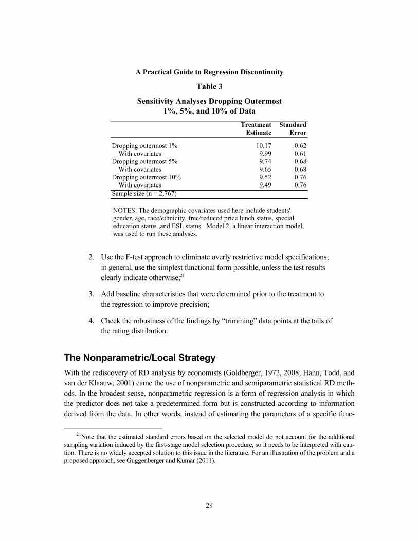
We then run the Model 2 again, but this time we drop the outermost 1 percent, 5 per-cent, and 10 percent of the data points. The results are shown in Table 3. We see that as we suc-cessively drop points, the standard error of the estimate increases, but that the impact estimate hovers around the true impact of 10 points. Remember that the standard deviation on this varia-ble is approximately 15 points, so a difference of 0.5 points (between the original model and the one in which 10 percent of the data points on either side of the cut-point have been dropped) translates to a difference in effect size of 0.03 — a very small difference. This suggests that Model 2 is a good choice.
Recommendations We recommend that the analyst take the following steps when conducting parametric analyses:
18Note that dropping 5 percent or 10 percent of the data points can result in a significant loss of statistical
power due to the smaller sample sizes, and thus results that were statistically significant when the full range of data were used may no longer be statistically significant. Researchers should be concerned with whether or not the point estimate changes substantially when the outermost points are dropped and not with whether or not the results remain statistically significant.
19The demographic covariates used here include students’ gender, age, race/ethnicity, free/reduced price lunch status, special education status, and ESL status.
20Also note that adding covariates to the model reduces the standard error of the estimate for all models presented in Table 2, therefore improving the precision of the model. However, the reduction in standard error is quite small in this example: For Model 2, adding the covariates reduces the standard error of treatment effect estimate from 0.590 to 0.585.
26
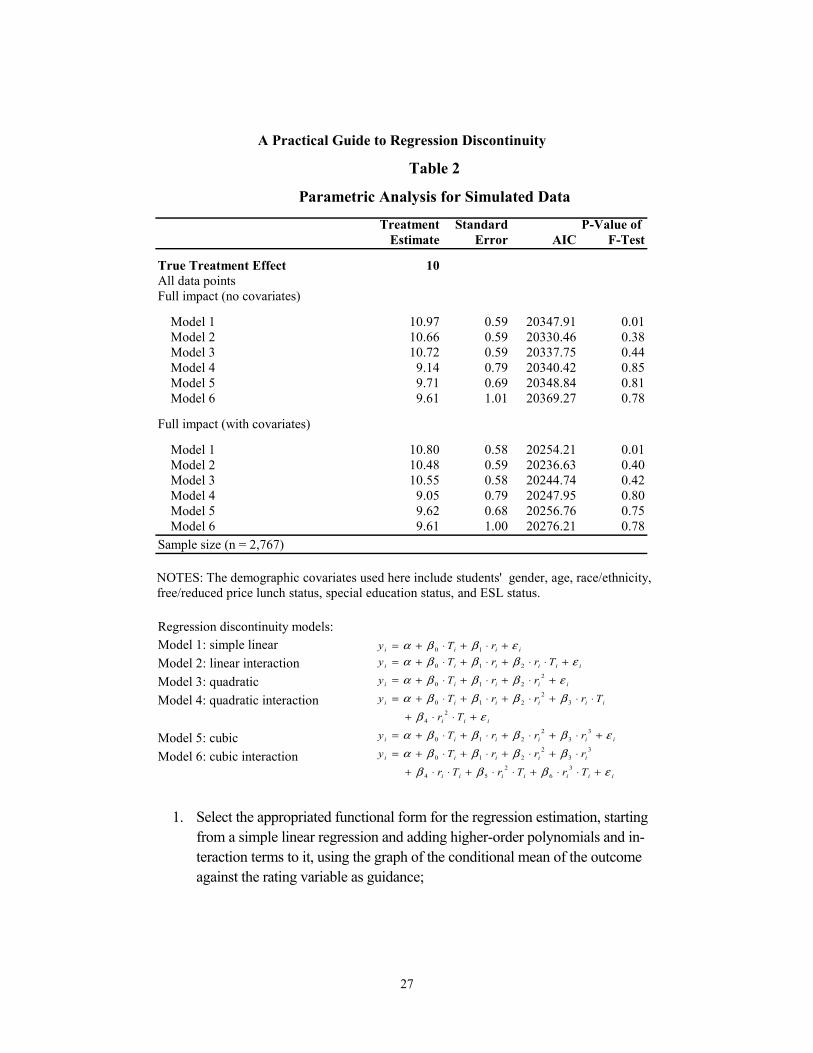
1. Select the appropriated functional form for the regression estimation, starting from a simple linear regression and adding higher-order polynomials and in-teraction terms to it, using the graph of the conditional mean of the outcome against the rating variable as guidance;
Treatment Standard P-Value of Estimate Error AIC F-Test
10
10.97 0.59 20347.91 0.0110.66 0.59 20330.46 0.3810.72 0.59 20337.75 0.44
9.14 0.79 20340.42 0.859.71 0.69 20348.84 0.819.61 1.01 20369.27 0.78
10.80 0.58 20254.21 0.0110.48 0.59 20236.63 0.4010.55 0.58 20244.74 0.42
9.05 0.79 20247.95 0.809.62 0.68 20256.76 0.759.61 1.00 20276.21 0.78
Regression discontinuity models:Model 1: simple linear Model 2: linear interactionModel 3: quadraticModel 4: quadratic interaction
Model 5: cubicModel 6: cubic interaction
Table 2
Parametric Analysis for Simulated Data
True Treatment EffectAll data points
A Practical Guide to Regression Discontinuity
Full impact (with covariates)
Full impact (no covariates)
Sample size (n = 2,767)
Model 3Model 2Model 1
Model 5Model 4Model 3Model 2Model 1
Model 6
Model 6Model 5Model 4
NOTES: The demographic covariates used here include students' gender, age, race/ethnicity, free/reduced price lunch status, special education status, and ESL status.
iiiiiii
iiiii
iiiiii
iii
iiiiii
iiiii
iiiiii
iiii
TrTrTr
rrrTy
rrrTy
Tr
TrrrTy
rrTy
TrrTy
rTy
εβββββββα
εββββαεβ
ββββαεβββα
εβββαεββα
+⋅⋅+⋅⋅+⋅⋅+
⋅+⋅+⋅+⋅+=
+⋅+⋅+⋅+⋅+=
+⋅⋅+
⋅⋅+⋅+⋅+⋅+=
+⋅+⋅+⋅+=
+⋅⋅+⋅+⋅+=+⋅+⋅+=
36
254
33
2210
33
2210
24
32
210
2210
210
10
27
2. Use the F-test approach to eliminate overly restrictive model specifications;
in general, use the simplest functional form possible, unless the test results clearly indicate otherwise;21
3. Add baseline characteristics that were determined prior to the treatment to the regression to improve precision;
4. Check the robustness of the findings by “trimming” data points at the tails of the rating distribution.
The Nonparametric/Local Strategy With the rediscovery of RD analysis by economists (Goldberger, 1972, 2008; Hahn, Todd, and van der Klaauw, 2001) came the use of nonparametric and semiparametric statistical RD meth-ods. In the broadest sense, nonparametric regression is a form of regression analysis in which the predictor does not take a predetermined form but is constructed according to information derived from the data. In other words, instead of estimating the parameters of a specific func-
21Note that the estimated standard errors based on the selected model do not account for the additional
sampling variation induced by the first-stage model selection procedure, so it needs to be interpreted with cau-tion. There is no widely accepted solution to this issue in the literature. For an illustration of the problem and a proposed approach, see Guggenberger and Kumar (2011).
Treatment StandardEstimate Error
10.17 0.629.99 0.619.74 0.689.65 0.689.52 0.769.49 0.76
Sample size (n = 2,767)
Table 3
A Practical Guide to Regression Discontinuity
Sensitivity Analyses Dropping Outermost1%, 5%, and 10% of Data
With covariates
With covariates
With covariatesDropping outermost 1%
Dropping outermost 5%
Dropping outermost 10%
NOTES: The demographic covariates used here include students' gender, age, race/ethnicity, free/reduced price lunch status, special education status ,and ESL status. Model 2, a linear interaction model, was used to run these analyses.
28

tional form (as one would do in the case of linear regression), one would estimate the functional form itself.22
In the RD context, the simplest nonparametric approach involves choosing a small neighborhood (known as bandwidth or discontinuity sample) to the left and right of the cut-point and using only data within that range to estimate the discontinuity in outcomes at the cut-point. A straightforward way to estimate treatment effects in this context is to take the differ-ence between mean outcomes for the treatment and control bins immediately next to the cut-point. This is consistent with the view of RD as local randomization.
However, the simple nonparametric approach of comparing means in the two bins adja-cent to the cut-point is generally biased in the neighborhood of the cut-point.23 Figure 5 illus-trates this problem for a downward-sloping regression function with no treatment effect (the solid curve). The figure focuses on two bins of equal bandwidth (h) located immediately to the left and right of a cut-point. Point A represents the mean outcome (in expectation) for the con-trol bin, and point B represents the mean outcome (in expectation) for the treatment bin. There-fore ( ∗ − ∗) equals the expected value of the estimated treatment effect. This value is posi-tive, even though the intervention has no effect. Hence, using the means for the two bins with bandwidth h immediately to the right and left of the cut-point produces a biased estimator. As the bandwidth decreases, the bias decreases, but it can still be substantial.
To reduce this boundary bias, it is recommended that instead of using a simple differ-ence of means, local linear regression (Hahn, Todd, and van der Klaauw, 2001) be used.24 In the context of an RD analysis, as noted earlier, local linear regression can simply be thought of as estimating a linear regression on the two bins adjacent to the cut-point, allowing the slope and intercept to differ on either side of the cut-point. This is equivalent to estimating impacts on a subset of the data within a chosen bandwidth h to the left and right of the cut-point, using the following regression model:
= + ∙ + ∙ + ∙ ∙ +
22For a comprehensive review of the nonparametric approach in general, see Härdle and Linton (1994) or
Pagan and Ullah (1999). 23These poor boundary properties are well documented in the nonparametric literature. See, for example,
Fan (1992) and Härdle and Linton (1994). 24Partial linear or local polynomial regression can also be used (Porter, 2003).
29
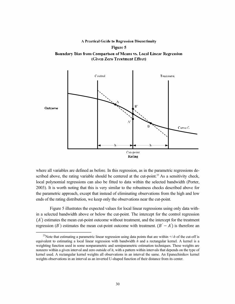
where all variables are defined as before. In this regression, as in the parametric regressions de-scribed above, the rating variable should be centered at the cut-point.25 As a sensitivity check, local polynomial regressions can also be fitted to data within the selected bandwidth (Porter, 2003). It is worth noting that this is very similar to the robustness checks described above for the parametric approach, except that instead of eliminating observations from the high and low ends of the rating distribution, we keep only the observations near the cut-point.
Figure 5 illustrates the expected values for local linear regressions using only data with-in a selected bandwidth above or below the cut-point. The intercept for the control regression ( ′) estimates the mean cut-point outcome without treatment, and the intercept for the treatment regression ( ′) estimates the mean cut-point outcome with treatment. ( ′ − ′) is therefore an
25Note that estimating a parametric linear regression using data points that are within +/-h of the cut-off is equivalent to estimating a local linear regression with bandwidth h and a rectangular kernel. A kernel is a weighting function used in some nonparametric and semiparametric estimation techniques. These weights are nonzero within a given interval and zero outside of it, with a pattern within intervals that depends on the type of kernel used. A rectangular kernel weights all observations in an interval the same. An Epanechinikov kernel weights observations in an interval as an inverted U-shaped function of their distance from its center.
30

estimate of the treatment effect, which is nonzero and thus biased, because the functional form is still not totally correct within the bandwidth. However, its bias is much smaller than that of the simple difference in means.
Challenges and Solutions While it is straightforward to estimate a linear or polynomial regression within a given window of bandwidth h around the cut-point, it is challenging to choose this bandwidth. In general, choosing a bandwidth in nonparametric estimation involves finding an optimal balance between precision and bias: While using a larger bandwidth yields more precise estimates, since more data points are used in the regression, as demonstrated above, the linear specification is less likely to be accurate, which can lead to bias when estimating the treatment effect.
Two procedures for choosing an optimal bandwidth for nonparametric regressions have been proposed in the literature and used for RD designs. The first is a cross-validation proce-dure; the second “plugs-in” a “rule-of-thumb” bandwidth and parameter estimates from the data into an optimal bandwidth formula to get the desired bandwidth. Both procedures are based on the concept of mean square error (MSE), which measures the trade-off between bias and preci-sion in the various models. As the bandwidth gets bigger, the estimates are more precise, but the potential for bias is also larger. Both procedures are also computationally complicated. In what follows, we briefly describe the basic concepts of each procedure and introduce existing pro-grams that can be employed to implement them. We then use the simulated data to demonstrate how each of them works with real data.
The Cross-Validation Procedure
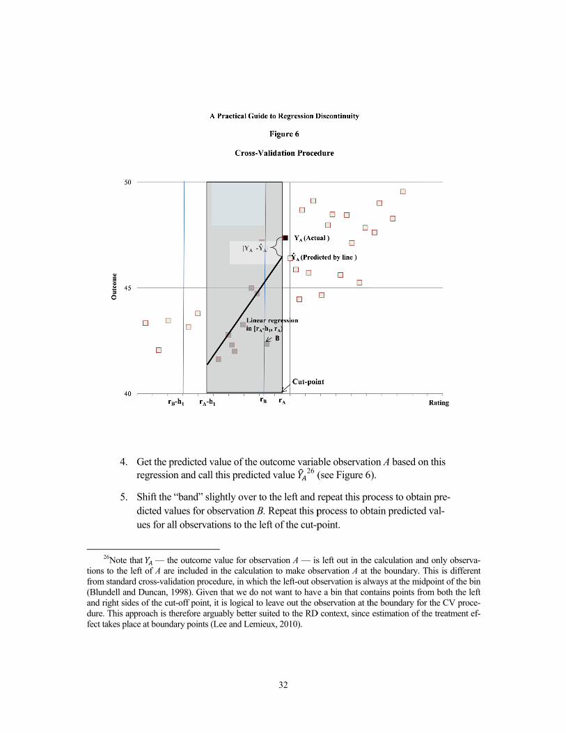
The first formal way of choosing the optimal bandwidth, which is used widely in the literature, is called the “leave-one-out” cross-validation procedure. Recently, Ludwig and Miller (2005) and Imbens and Lemieux (2008) have proposed a version of the “leave-one-out” cross-validation procedure that is tailored for the RD design. This cross-validation procedure can be carried out as follows (a visual depiction of this procedure is shown in Figure 6):
1. Select a bandwidth ℎ . 2. Start with an observation A to the left of the cut-point, with rating and an
outcome .
3. To see how well the parametric assumption fits the data within the bandwidth ℎ , run a regression of the outcome on the rating using all of the observations that are located to the left of observation A and have a rating that ranges from − ℎ to (not including ).
31
2
tions from (Blunand ridure. fect ta
4. Get thregres
5. Shift dictedues fo
26Note that —to the left of Astandard cross-
ndell and Duncaight sides of theThis approach
akes place at bo
he predicted vssion and call
the “band” sld values for oor all observat
— the outcome A are included i-validation procan, 1998). Givee cut-off point, is therefore arg
oundary points (
value of the ol this predicte
lightly over toobservation B.tions to the le
value for obse
in the calculatiocedure, in whichen that we do nit is logical to
guably better su(Lee and Lemie
utcome variaed value 26 (
o the left and r Repeat this p
eft of the cut-p
ervation A — ison to make obsh the left-out ob
not want to haveleave out the o
uited to the RDeux, 2010).
able observati(see Figure 6
repeat this prprocess to obtpoint.
s left out in theservation A at tbservation is alwe a bin that con
observation at thD context, since
ion A based on).
rocess to obtatain predicted
e calculation anthe boundary. Tways at the midntains points frohe boundary foestimation of t
n this
ain pre-d val-
nd only observaThis is differendpoint of the binom both the lef
or the CV procethe treatment ef
a-nt n ft e-f-
32

6. Then repeat this process to obtain predicted values for all observations to the right of the cut-point; stop when there are fewer than two observations be-tween − ℎ and ri.
7. Calculate the cross-validation criterion (CV) — in this case, the mean square error — for bandwidth ℎ using the following formula:
(ℎ ) = 1 ( − )
where N is the total number of observations in the data set and all other variables are as defined before.
8. Repeat the above steps for other bandwidth choices ℎ , ℎ , ….
9. Pick the bandwidth that minimizes the cross-validation criterion, that is, pick the bin width that produces the smallest mean square error.
Writing a program to carry out this cross-validation procedure is not difficult and can be accomplished with most statistical software packages. However, the process is largely data-driven and can be time-consuming.
The “Plug-In” Procedure
This procedure describes (using a mathematical formula) the optimal bandwidth in terms of characteristics of the actual data, with the goal of balancing the degree of bias and pre-cision. Intuitively, this formula provides a closed form analytic solution for the bandwidth that minimizes a particular function of bias and precision. Fan and Gijbels (1996) developed this method in the context of local linear regressions, and both Imbens and Kalyanaraman (2009) and DesJardins and McCall (2008) have adapted and modified it for the RD setting.
The formula for the optimal bandwidth in a RD design is the following (Equation 4.7 in Imbens and Kalyanaraman, 2009):
ℎ = ∙ ( 2 ∙ ( )/ ( )( ( )( ) − ( )( )) + ( ̂ + ̂ )) ∙
where is a constant specific to the weighting function in use;27 is the cut-point value; ( ) is the estimated conditional variance function of the rating variable at the cut-point; ( ) is the estimated density function of the rating variable at the cut-point; ( )( ) as well as ( )( ) is
27In our example, this is a rectangular kernel.
33

the second derivative of the relationship between the outcome and the rating; and ̂ + ̂ is the regularization term to the denominator in the equation to adjust for the potential low precision in estimating the second derivatives.28 N is the number of observations available.
To implement this procedure, one first needs to use a starting rule to get an initial “pi-lot” bandwidth.29 The conditional density function ( )and the conditional variance ( ) are then estimated based on data within the pilot bandwidth on both side of the cut-point c. Similar-ly, the second derivatives ( )( ), ( )( ) as well as the regularization term ̂ + ̂ will also be estimated based on the pilot bandwidth. Once all these pieces are estimated, one can plug them into the formula and compute the optimal bandwidth.
The procedure is computationally intensive. Fortunately, software programs for imple-menting this procedure are available from Imbens’ Web site.30
Both the “plug-in” and the cross-validation procedures described above are tailored for the RD design. Simulation results reported by Imbens and Kalyanaraman (2009) show that even though the two procedures tend to produce different bandwidth choices, the impact estimates based on these bandwidths are not quantitatively different from each other in the cases they ex-amine. A recent U.S. Department of Education, Institute for Education Sciences, report on RD designs found similar results (Gleason, Resch, and Berk, 2012).
Illustration We use the simulated data set to illustrate the implementation of the two methods for bandwidth selection. First we use the cross-validation approach to identify a choice of bandwidth. Table 4 shows the cross-validation criterion — the mean square error (MSE) — associated with a wide range of bandwidth choices. These cross-validation results indicate that a bandwidth of 12 seems to minimize the cross-validation criterion and therefore should be the optimal bandwidth choice.
Then we use the program provided by Imbens and Kalyanaraman (2009) to determine the optimal bandwidth based on the “plug-in” method. This method suggests that the optimal bandwidth is 9.92.
Next, we estimate the treatment effect based on these two bandwidth choices using the following models:
28For derivation of the formula, see Imbens and Kalyanaraman (2009). 29The rule used by Imbens and Kalyararaman (2009) is ℎ = 1.84 ∙ ∙ ⁄ where the sample variance
of the rating variable is equal to = ∑( − ) /( − 1). 30http://www.economics.harvard.edu/faculty/imbens/software_imbens.
34

1. linear = + ∙ + ∙ +2. linear interaction = + ∙ + ∙ + ∙ ∙ + 31 3. quadratic = + ∙ + ∙ + ∙ + 4. quadratic interaction = + ∙ + ∙ + ∙ + ∙ ∙ + ∙∙ +
Table 5 reports the estimation results for the two bandwidth choices and the four mod-els. The first two columns report the point estimates and standard errors. The Akaike Infor-mation Criterion (AIC) and F-test is also reported for the purpose of comparison. We can see that, consistent with the finding of Imbens and Kalyanaraman (2009), both bandwidth choices yield very similar results in terms of their estimated impact, and the estimated impact in both cases is quite close to the true impact of 10 points. This suggests that either method will effec-tively identify an appropriate bandwidth. Looking within each bandwidth, we see that Model 1 has the lowest standard error. As will be described in more detail in the section on precision be-
31This model is equivalent to running local linear regression using a rectangular kernel.
Bandwidth N MSE
1 2,767 106.513 2,767 106.375 2,767 106.887 2,767 106.759 2,767 105.47
10 2,767 105.3111 2,767 105.2512 2,767 104.9813 2,766 105.5714 2,767 105.6215 2,767 106.0720 2,766 106.0530 2,767 104.8445 2,767 104.57
A Practical Guide to Regression Discontinuity
Cross-Validation Criteria for Various Bandwidths
Table 4
35
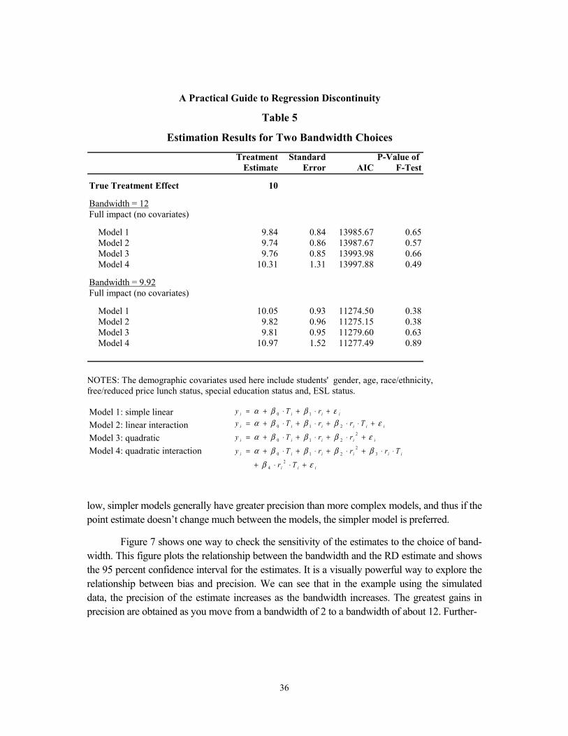
low, simpler models generally have greater precision than more complex models, and thus if the point estimate doesn’t change much between the models, the simpler model is preferred.
Figure 7 shows one way to check the sensitivity of the estimates to the choice of band-width. This figure plots the relationship between the bandwidth and the RD estimate and shows the 95 percent confidence interval for the estimates. It is a visually powerful way to explore the relationship between bias and precision. We can see that in the example using the simulated data, the precision of the estimate increases as the bandwidth increases. The greatest gains in precision are obtained as you move from a bandwidth of 2 to a bandwidth of about 12. Further-
Treatment Standard P-Value of Estimate Error AIC F-Test
True Treatment Effect 10
Model 1 9.84 0.84 13985.67 0.65Model 2 9.74 0.86 13987.67 0.57Model 3 9.76 0.85 13993.98 0.66Model 4 10.31 1.31 13997.88 0.49
Model 1 10.05 0.93 11274.50 0.38Model 2 9.82 0.96 11275.15 0.38Model 3 9.81 0.95 11279.60 0.63Model 4 10.97 1.52 11277.49 0.89
Model 1: simple linear Model 2: linear interactionModel 3: quadraticModel 4: quadratic interaction
Full impact (no covariates)Bandwidth = 9.92
A Practical Guide to Regression Discontinuity
Full impact (no covariates)Bandwidth = 12
Estimation Results for Two Bandwidth Choices
Table 5
NOTES: The demographic covariates used here include students' gender, age, race/ethnicity, free/reduced price lunch status, special education status and, ESL status.
iii
iiiiii
iiiii
iiiiii
iiii
Tr
TrrrTy
rrTy
TrrTy
rTy
εβ
ββββα
εβββα
εβββαεββα
+⋅⋅+
⋅⋅+⋅+⋅+⋅+=
+⋅+⋅+⋅+=
+⋅⋅+⋅+⋅+=+⋅+⋅+=
24
32
210
2210
210
10
36
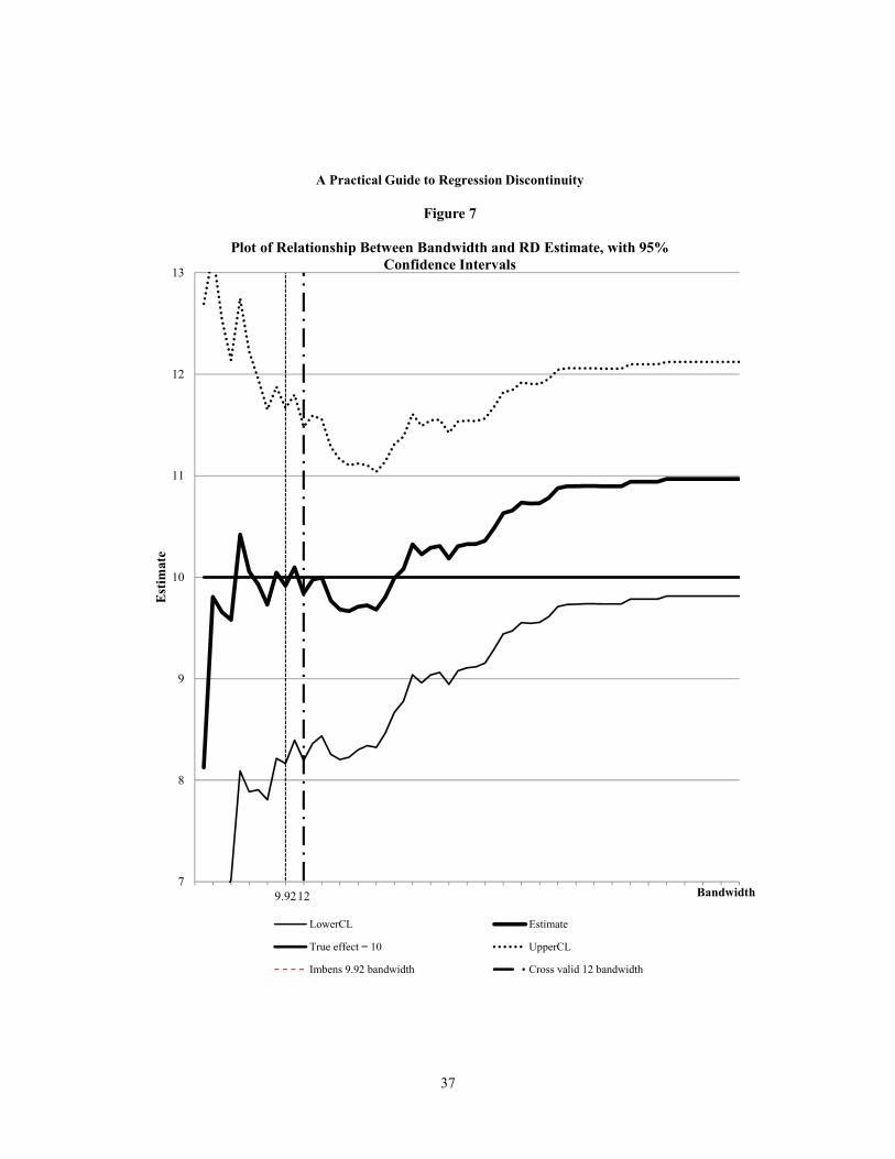
7
8
9
10
11
12
13
9.9212
Estim
ate
Bandwidth
A Practical Guide to Regression Discontinuity
Figure 7
Plot of Relationship Between Bandwidth and RD Estimate, with 95% Confidence Intervals
LowerCL Estimate
True effect = 10 UpperCL
Imbens 9.92 bandwidth Cross valid 12 bandwidth
37
more, with bandwidth choices between 2 and 12, the estimate hovers right around the true im-pact of 10 points. If the bandwidth is expanded beyond 24, more consistently biased estimates result. This visual inspection confirms our choice of bandwidth somewhere between 9 and 12. Although in our simulated data, the true impact is known, a similar graph can be used to explore the implications of various bandwidth choices, even when the true impact is not known. And, of course, the results of doing so might differ from those in the present example.
Recommendations We recommend that analysts conducting local linear regression analyses use the following steps:
• Depending on computational capacity, use the “plug-in,” the cross-validation methods, or both to select an optimal bandwidth.
• Use linear regression to estimate the treatment effect based on the subset of data identified by the optimal bandwidth(s).
• Check the robustness of the findings by using local polynomial regressions; use the AIC or F-test to eliminate overly restrictive models.
• Check the sensitivity of the estimates by presenting a plot of the RD esti-mates and the associated 95 percent confidence intervals as a function of the bandwidth.
• Also provide parametric estimates as sensitivity checks.
• If the results of these sensitivity tests differ from the general results, present both and discuss the differences in the direction and magnitude of the effects as well as the power of the various models. If the primary difference is whether or not the tests are statistically significant, determine whether or not the difference is being driven by a change in the point estimates or an in-crease in the standard error, or both — changes that are driven by a large change in the point estimates are of greater concern. If the direction of the ef-fect differs, compare the results with a visual inspection of the graph of out-comes against ratings. If the magnitudes differ but the direction of the effect is the same, you can use the smaller impact as an informal lower bound of the potential effect.
38

Parametric versus Nonparametric Estimation So far, we have been discussing the parametric and nonparametric approaches separately. The two approaches make different choices regarding precision and bias. The parametric approach makes full use of available data at the risk of generating biased estimates based on inaccurate model specification. The nonparametric approach, however, sacrifices precision by limiting the analysis to only a subset of observations that are close enough to the cut-point in order to more accurately specify the functional form and hence reduce (but perhaps not eliminate) bias in es-timation.
The two approaches also behave differently as the sample size goes to infinity. With an infinitely large sample, a parametric approach can still produce biased yet precisely estimated results, because, in this case, the degree of bias is determined by the functional form that is se-lected. In contrast, as the sample size goes to infinity in the nonparametric model, the optimal bandwidth will shrink, and the observations used in a nonparametric regression will get infinite-ly close to the cut-point, causing the amount of bias to approach zero as well (Lee and Lemieux, 2010).32
At the same time, there need not be a strict distinction between these two approaches: One can easily morph into the other if viewed from a slightly different angle. For example, the parametric approach can be viewed as nonparametric with a very large bandwidth — so large that it essentially includes all available observations. Similarly, the nonparametric approach can be viewed as a parametric regression on a subset of the full data set. Furthermore, if one wanted to exclude the influence of data points in the tails of the rating distribution, one could call the exact same procedure “parametric” after trimming the tails, or “nonparametric” by viewing the restriction in the range of rating as a result of using a smaller bandwidth.
Therefore, in practice, it is not important to make a clear distinction between these two approaches. Rather, we recommend providing estimates using all plausible combinations of specifications of the functional form and the bandwidth. Specifically, if the sample size is small, especially if there is not a critical mass of data points around the cut-point, consider using para-metric estimation as the primary estimation method to make use of all data points and present nonparametric estimates as “complementary” results. At the same time, if the sample size is large, particularly around the cut-point, consider using nonparametric estimation as the primary method, since precision is less of a concern in this situation, and then provide parametric esti-mates as sensitivity checks.
Results that are stable across all plausible specifications of the functional form and bandwidth can be considered more robust and reliable than those that are sensitive to specifica-
32This will result in consistent but not unbiased estimates.
39
tions. Looking back at Tables 2 and 5, for the simulated data set, both approaches provide esti-mates that hover around the true effect of 10, indicating robust findings.
Now that we have outlined the steps for estimation in an RD design and laid the groundwork for understanding the complexities of RD estimation, we turn to a discussion of a number of issues related to RD designs, including how to establish the internal validity of an RD design, the precision of estimators in a RD design, and the generalizability of RD results. We begin with a discussion of internal validity.
40
5 Establishing the Internal Validity of Regression Discontinuity Impact Estimates33
A RD design is considered to be internally valid if a valid causal interference can be made for the sample that is being observed, as opposed to the population to which these findings will be generalized. (Shadish, Cook, and Campbell, 2002). Without establishing the internal validity of the RD design, no causal interpretation can be made. While a valid RD design can identify a treatment effect in much the same way a randomized trial does, in order for an RD design to be valid, a clear discontinuity in the probability of receiving treatment must exist at the cut-point, and candidates’ ratings and the cut-point must be determined independently of each other. This condition can be ensured if the cut-point is determined without knowledge of candidates’ rat-ings and if candidates’ ratings are determined without knowledge of the cut-point.34 If not, the internal validity of the RD design is called into question.
On the one hand, if the cut-point is to be chosen in the presence of knowledge about candidates’ ratings, decision makers can locate the cut-point in a way that includes or excludes specific candidates. If the selected and nonselected candidates are different in systematic ways from one another, those on one side of the cut-point will not provide valid information about the counterfactual outcome for those on the other side. This situation could arise, for example, when a fixed sum of grant funding is allocated to a pool of candidates, and average funding per recipient is determined in light of knowledge about candidates’ ratings. With a fixed total budg-et, average funding per recipient determines the number of candidates funded, which in turn determines the cut-point. Through this mechanism, the cut-point could be manipulated to in-clude or exclude specific candidates.
On the other hand, if ratings are determined in the presence of knowledge about the cor-responding cut-point, they can be manipulated to include or exclude specific candidates. For example, if a college’s admissions director were the only person who rated students for admis-sion, he could fully determine whom to accept and whom to reject by setting ratings according-ly. Consequently, students accepted could differ from those rejected in ways unobserved by the researcher, and their counterfactual outcomes would differ accordingly. A second possible ex-ample is one in which students must pass a test to avoid mandatory summer school, and they know the minimum passing score. In this case, students who are at risk of failing but sufficient-ly motivated to work extra hard might be especially prevalent among just-passing scores, and students with similar aptitude but less motivation might be especially prevalent among just-
33Much of the introduction to this section was adapted from Bloom (2012). 34This is a sufficient condition.
41

failing scores. The two groups, therefore, will not provide valid information about each other’s counterfactual outcomes.
Lee (2008) and Lee and Lemieux (2010) provide an important insight into the likeli-hood of meeting the necessary condition for a valid RD design. They do so by distinguishing between situations with precise control over ratings (which are rare) and situations with impre-cise control over ratings (which are typical). Precise control means that candidates or decision makers can determine the exact value of each rating. This was assumed to be the case in the preceding two examples, where a college admissions director could fully determine applicants’ ratings, or individual students could fully determine their test scores.
The situation is quite different, however, when control over ratings is imprecise, which would be the case in more realistic versions of the preceding examples. Most colleges have multiple members of an admissions committee rate each applicant, and thus no single individual can fully determine a student’s rating. Consequently, applicant ratings contain random variation due to differences in raters’ opinions and variation in their opinions over time. Also, because of random testing error, students cannot fully determine their scores on a test.35 Lee (2008) and Lee and Lemieux (2010) demonstrate that such random variation is the sole factor determining which candidates fall just below and above a cut-point. They thereby demonstrate that impre-cise control over ratings is sufficient to produce random assignment at the cut-point, which yields a valid RD design, as long as the cut-point is not chosen with knowledge of the candi-dates’ ratings.
Basic Steps There are a variety of approaches that researchers can use to determine whether or not ratings or cut-points could have been manipulated (that is, whether or not a RD discontinuity design is internally valid).
Understand the Ratings Process
The first step is for the researchers to learn as much as possible about how the ratings were assigned and how the cut-point was chosen. This can be accomplished by talking with those involved in the rating process and those who were involved in determining the cut-point. In other cases, a document review can provide the necessary information. For example, re-searchers could review program application materials and the description of how the “winners” would be selected and then compare this information with the list of actual winners to see whether the two were consistent with one another. In all cases, the researcher should take care
35For example, students can misread questions or momentarily forget things they know.
42
to document the information obtained about the process for rating subjects and determining the cut-point.
Even in cases where all the evidence seems to suggest that the design is a valid one, re-searchers should also objectively assess whether or not the design meets the qualifications for an internally valid RD design, since it is always possible that some manipulation may have oc-curred. At the same time, even if there is some evidence of potential manipulation, if individuals do not have complete control over the ratings, then the design may still be valid. Here we out-line the various statistical approaches that can be used to assess the validity of an RD design.
Probability of Receiving Treatment
Researchers should examine a graph plotting the probability of receiving treatment as a function of the rating variable. The steps outlined above for implementing a graphical analysis can be followed for this and all graphs discussed in this section. For a valid RD design, there should be a discontinuity (or “jump”) at the cut-point in the probability of receiving treatment. If this discontinuity is 1 ― in other words, if all observations to one side of the cut-point received the treatment while all observations to the other side of the cut-point did not ― then the RD de-sign is a “sharp” RD design. If this discontinuity is somewhere between 0 and 1, that is, if some observations that should have received treatment did not (“no-shows”), while some that should not have received treatment did (“crossovers”), then the RD design is a “fuzzy” design. In this case, the RD design still meets the conditions for validity but, as will be described later, adjust-ments will be necessary to recover the treatment effect. At the same time, if there is no “jump” in the probability of receiving treatment at the cut-point, then there is no treatment contrast to be tested, and the usefulness of the design is called into question.
Examine Nonoutcome Variables
Next, we recommend creating graphs that plot the relationship between nonoutcome variables and the rating variable. Nonoutcome variables here refer mainly to potential covariates that, according to the theory of action, should not be affected by the treatment. For example, in a school-based intervention for students in grades K-3, with student achievement as the outcome of interest, one would not expect fourth-grade scores in the first year of the treatment to be im-pacted by the treatment. If the ratings or cut-point were manipulated in some way, then this might be reflected in a discontinuity at the cut-point for the fourth-grade scores. This might oc-cur if the ratings were manipulated so that a few organized and highly motivated schools that did not officially meet the requirements for inclusion in the treatment group were included any-way. As a result, the fourth-grade test scores might show a discontinuity at the cut-point, with the fourth-graders in the treatment schools scoring higher than those in the control schools. De-mographic characteristics of the groups or individuals involved in the study are also good can-
43

didates to explore. An example using our simulated data set is shown in Figure 8. In this figure, we plot the rating against student age (a variable that should not be impacted by any interven-tion), using a bin size of 3 (the same bin size used for the initial graphical analysis of the data). We see that there is no discontinuity in student age around the cut-point in our example, lending support to the notion that this a valid RD design. This analysis could also be conducted in a re-gression framework, rather than graphically.
In conducting these graphical analyses, any observed discontinuity in variables that should not be impacted by the treatment calls into question the validity of the RD design. How-ever, even if the selected variables show no evidence of a discontinuity at the cut-point, this does not mean that the design is internally valid. It is possible that the manipulation that oc-curred simply had no impact on the nonoutcome variable. Thus, it is important to conduct this test on as wide a range of baseline characteristics of sample members as is possible given the data that are available. Furthermore, in some instances, appropriate variables are not available to researchers to conduct such tests, so other alternatives for assessing the internal valid of an RD design are needed.
Density of the Rating Variable
Another approach that is frequently used is to visually inspect a graph of the density of the rating variable (that is, a graph in which the rating is plotted against the number of observa-tions at each point along the rating scale). If the RD design is valid (that is, there was no manip-ulation around the cut-point), then there should be no discontinuity observed in the number of observations just above or below the cut-point. If, however, there is a sharp increase in the number of observations either right above or right below the cut-point, it suggests that either the placement of the cut-point or the ratings themselves have somehow been manipulated. Say, for example, there was a program in which student scores on an exam were used to determine eli-gibility — students achieving a certain score on the test would be granted admission and those missing the cut-point would not. If the teachers who were administering the test knew the test score that was being used to determine eligibility, they might be inclined to give students they thought were worthy of inclusion in the program slightly higher scores. This would be reflected in a sharp increase in the number of students just above the cut-point.
Figure 9 shows what the density of the rating variable might look like in the presence of manipulation around the cut-point. While a visual inspection of this graph clearly indicates a discontinuity at the cut-point, in other instances the discontinuity may not be as easily deter-mined through visual inspection.
McCrary (2008) offers a formal empirical test of this phenomenon that assesses wheth-er the discontinuity in the density of the ratings variable at the cut-point is equal to zero. The following outlines the steps for implementing this test:
44
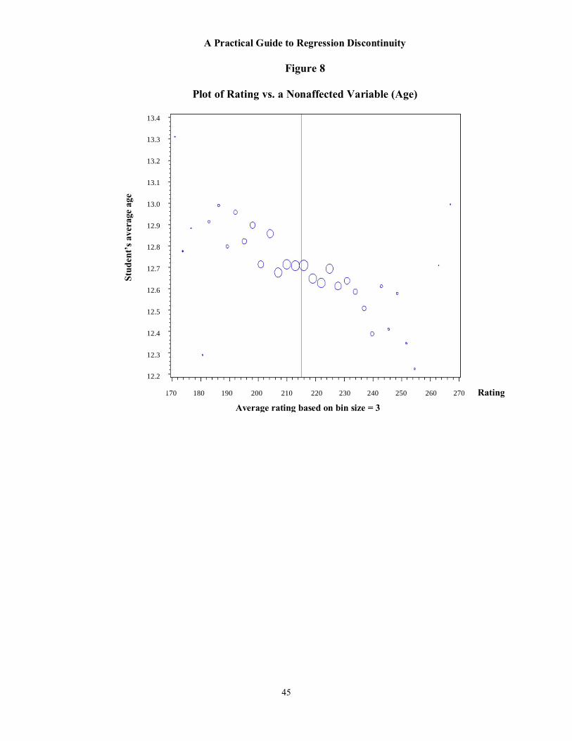
A Practical Guide to Regression Discontinuity
Figure 8
Plot of Rating vs. a Nonaffected Variable (Age)
Average rating based on bin size = 3
Stud
ent’s
ave
rage
age
170 180 190 200 210 220 230 240 250 260 270 Rating
13.4 13.3 13.2 13.1 13.0 12.9 12.8 12.7 12.6 12.5 12.4 12.3 12.2
45
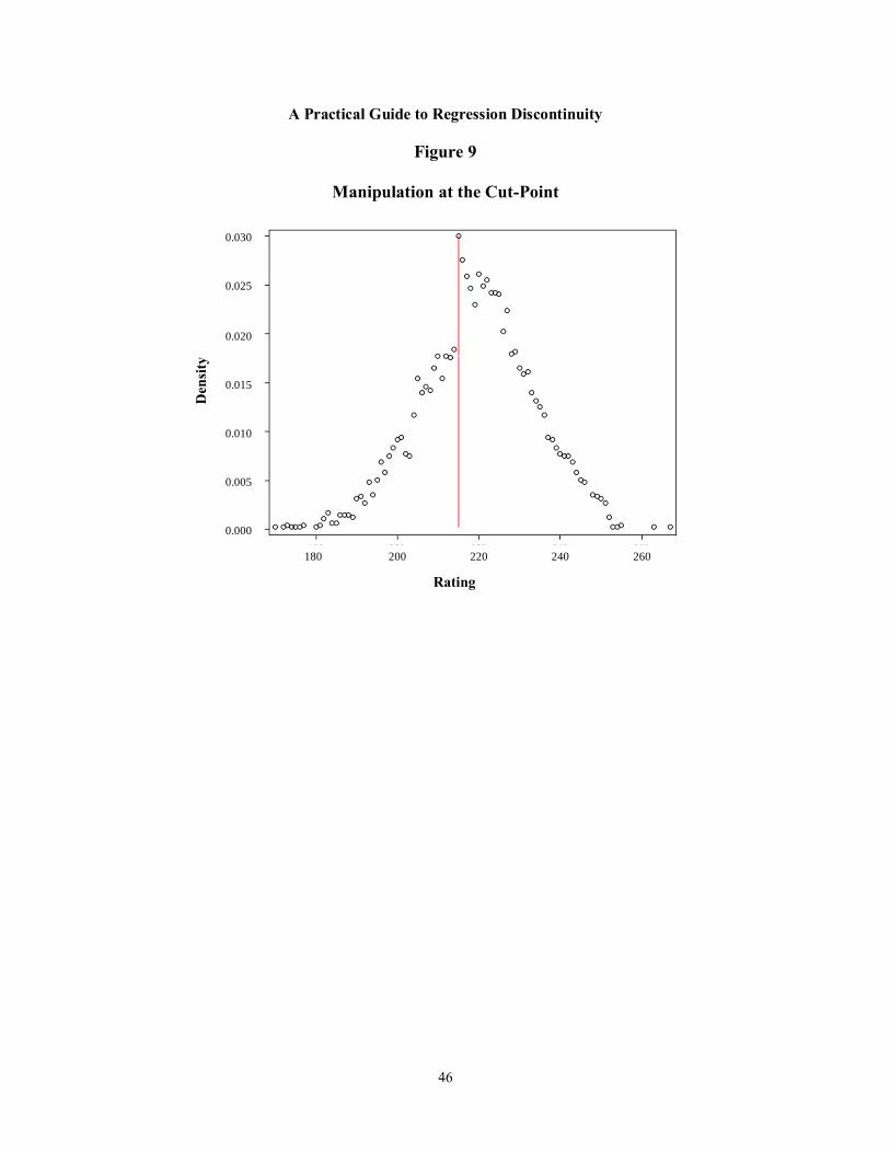
A Practical Guide to Regression Discontinuity
Figure 9
Manipulation at the Cut-Point
Rating
Den
sity
180 200 220 240 260
0.030
0.025
0.020
0.015
0.010
0.005
0.000
46
1. Create a histogram of the density of the rating using a particular bin size, en-suring that no bin overlaps the cut-point.
2. Run two local linear regressions, one to the right and one to the left of the cut-point. In these regressions the midpoint rating values of each of the bins are the regressors, and the frequency counts of each bin constitute the out-comes.
3. Test whether or not the log difference in height just to the right and just to the left of the cut-point (or the log difference of the intercepts of the two regres-sions) is statistically different from zero.
McCrary provides Stata code on his Web site for implementing this density test.36
Challenges and Solutions As with the graphical analyses described above, the most important decisions to be made when conducting this analysis are the choice of bin size (the number of ratings included for each point in the histogram) and bandwidth (the range of points which will be included in the local linear regressions). McCrary’s program uses default settings for the bin size and bandwidth.37 Howev-er, as he stresses in his paper, these are only starting values for determining the optimal bin size and bandwidth, and both visual inspection of the graphs and an automatic procedure, such as cross-validation, should be used to determine the optimal bin size and bandwidth. This is partic-ularly important in situations in which the rating variable is not continuous, as is the case with our simulated data set. In our data set, scores are all integers, so it is not possible to score be-tween 215 and 216, for example. The default bin width in the McCrary program is 0.49, which is meaningless in our data and leads to misleading results.38
When we use the techniques we recommended in the section on graphical analysis to determine the appropriate bin size and set our bin size equal to 3, we find that the linear smooth-ing line matches closely with the plotted points (see Figure 10), and the log difference in heights to the right and left of the cut-point is not statistically significant, as we would expect. Thus, we recommend using the steps outlined in the section on graphical analysis above to determine the
36http://emlab.berkeley.edu/~jmccrary/ 37The formulas used to determine the starting values can be found in McCrary (2008) on p. 10. The band-
width is chosen based on the “rule of thumb” procedure described in more detail in the estimation section of this paper.
38Strictly speaking, these test scores are an example of a discrete, as opposed to a continuous rating varia-ble. See Lee and Card (2008) for a complete treatment of discrete rating variables in RD designs.
47
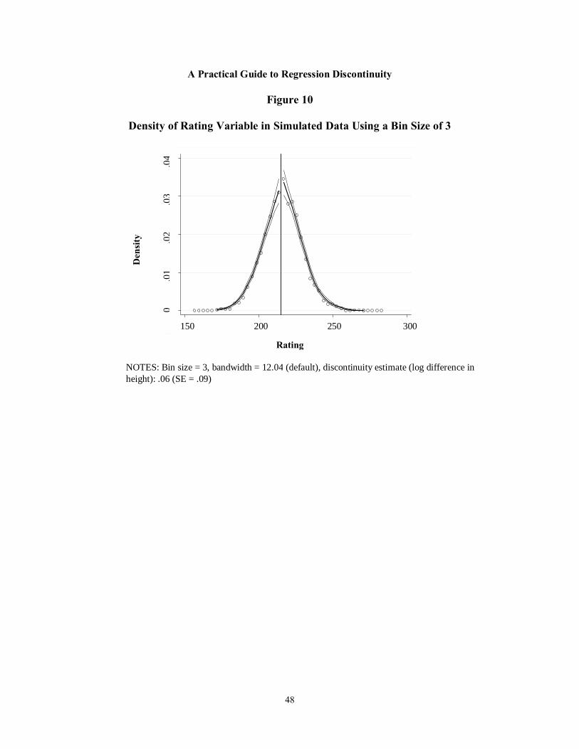
A Practical Guide to Regression Discontinuity
Figure 10
Density of Rating Variable in Simulated Data Using a Bin Size of 3
0.0
1.0
2.0
3.0
4
150 200 250 300
NOTES: Bin size = 3, bandwidth = 12.04 (default), discontinuity estimate (log difference in height): .06 (SE = .09)
0
.01
.
02
.03
.
04
150 200 250 300
Den
sity
Rating
48
optimal bin size, and then using that bin size, rather than the default values used in the McCrary test program, to run the analyses.
The McCrary test provides a useful diagnostic for assessing the internal validity of an RD design. However, it also has its weaknesses. First, because it is somewhat dependent on the choice of bin size and bandwidth, the exercise itself has a degree of subjectivity to it. Second, as McCrary notes, the test cannot identify a situation where manipulation has occurred in both di-rections (for example, some students were given higher test scores because it was thought that they would benefit from the treatment, and others were given lower scores because it was thought that they would be harmed by the treatment). If the number of students whose scores were adjusted up is equal to the number of students whose scores were adjusted down, the den-sity test will not show a discontinuity.39 In other words, the test can show whether or not the number of individuals assigned to a rating has a discontinuity, but it cannot show a discontinuity in the composition of the group.
Recommendations We recommend that researchers use all four techniques described here to assess whether or not their design is internally valid. Researchers should carefully document the process used to es-tablish the ratings and determine the cut-point, test a variety of variables that should not be af-fected by the treatment to see if any discontinuity occurs at the cut-point for these variables,40
visually inspect a graph of the density of the rating variable, and, finally, run the McCrary test. If all four methods suggest that there has been no manipulation of the ratings or the cut-point, then researchers can proceed with confidence. Ultimately, there is no way to know with certain-ty whether or not gaming has occurred at the cut-point without either controlling or fully know-ing how subjects were assigned to treatment.
39In technical terms, the density test only works if the manipulation is monotonic. 40Researchers should take multiple hypothesis testing into consideration when assessing the impact of the
intervention on nonoutcome variables. If 20 variables are tested, it is likely that one will be statistically signifi-cant by chance, and this should not raise any substantial concerns about the validity of the design.
49
6 Precision of Regression Discontinuity Estimates41
The next issue we consider is the precision of the estimates obtained from an RD design. This is something that is particularly relevant for those who are planning a study or are considering us-ing an RD design to estimate treatment effects in an existing data set. Researchers should pay particular attention to issues of precision, because, as we will demonstrate, the power to detect effects is considerably lower for an RD design than for a comparable randomized trial.
The precision of estimated treatment effects is typically expressed in terms of a mini-mum detectable effect (MDE) or a minimum detectable effect size (MDES). A minimum de-tectable effect is the smallest treatment effect that a research design has an acceptable chance of detecting if it exists. Minimum detectable effects are reported in natural units, such as scale-score points for standardized tests. A minimum detectable effect size is a minimum detectable effect divided by the standard deviation of the outcome measure. It is reported in units of stand-ard deviations.42
Formally, a minimum detectable effect (or effect size) is typically defined as the small-est true treatment effect (or effect size) that has an 80 percent chance (80 percent power) of pro-ducing an estimated treatment effect that is statistically significant at the 0.05 level for a two-sided hypothesis test. This parameter is a multiple of the standard error of the estimated treat-ment effect. The multiple depends on the number of degrees of freedom available (Bloom, 1995), but for more than about 20 degrees of freedom, its value is approximately 2.8.
Because most (parametric) RD analyses have more than 20 degrees of freedom, their minimum detectable effect (MDE) or minimum detectable effect size (MDES) can be approxi-mated as follows:43
≈ 2.8 ( )( )( ) (1)
41Much of the following section was adapted from Bloom (2012). 42Effect sizes are used to report treatment effects in education research, psychology, and other social sci-
ences (see, for example, Cohen, 1988; Rosenthal, Rosnow, and Rubin, 2000; and Grissom and Kim, 2005.) Choosing a target MDE or MDES requires considerable judgment and is beyond the scope of the present pa-per. Bloom, Hill, Black, and Lipsey (2008) and Hill, Bloom, Black, and Lipsey (2008) present an analytic ap-proach and empirical benchmarks for choosing minimum detectable effect sizes in education research.
43This expression is more complex for clustered RD designs (Schochet, 2008). The degree of complexity is parallel to that for clustered randomized trials (see, for example, Bloom, 2005, and Bloom, Richburg-Hayes, and Black, 2007).
50

≈ 2.8 ( )( )( ) (2)
where:
= The proportion of variation in the outcome (Y) predicted by the rating and oth-
er covariates included in the RD model
= The proportion of variation in treatment status (T) predicted by the centered rating and other covariates included in the RD model
= The total number of sample members
= The proportion of sample members in the treatment group
= The variance of the counterfactual outcome (that is, approximated by the out-come variance for the comparison group).
Impact estimates from an RD design generally have more limited power than other po-
tential designs. To gain some perspective on the precision of RD impact estimates, it is useful to compare the precision of a standard parametric RD design with that of a randomized trial. To make this comparison a fair one, assume that the two designs have the same total sample size (N), the same treatment/control group allocation (P vs. (1-P)), the same outcome measure (Y), and the same variance for the comparison group ( ). In addition, assume that the rating is the only covariate for the RD design and the randomized trial. (The rating might be a pretest used to increase a trial’s precision). Hence, the ability of the covariate to reduce unexplained variation in the outcome ( ) is the same for both designs.
A randomized trial with the rating as a covariate would use the same regression models as an RD design to estimate treatment effects. For example:
where:
= the outcome measure for observation i, = 1 if observation i is assigned to the treatment group and 0 otherwise, = the rating variable for observation i,
iiii rfTY εβα +++= )(0
iY
iT
ir
51

= a random error term for observation i, which is independently and identically distributed, with all terms defined as before. The MDE or MDES of the trial, therefore, can be expressed by (1) and (2) as well. The
only difference between the RD design and an otherwise comparable randomized trial is the value of , which is zero for a randomized trial and nonzero for an RD analysis. This differ-ence reflects the difference between the assignment processes of the two designs. The ratio of their minimum detectable effects or minimum detectable effect sizes is therefore:
= = (3)
represents the collinearity (or correlation squared) that exists between the treatment indicator and the (centered) rating in an RD design.44 This collinearity depends on how ratings are distributed around the cut-point (Goldberger, 1972, 2008; Bloom et al., 2005; and Schochet, 2008).
To illustrate, we can look at the for two types of distribution for the rating variable: a balanced uniform distribution and a balanced normal distribution. A uniform distribution would exist if ratings were expressed in rank order without ties. A normal distribution might exist if ratings were scores on a test, because test scores often follow a normal distribution. A balanced distribution is one that is centered on the cut-point, so that half of the observations are on one side and half are on the other side. The degree of imbalance of a distribution reflects its mix of treatment and comparison candidates. Figure 11 shows the two possible distributions of ratings.
To compute for a given distribution of ratings, one can generate ratings (r) from a distribution of interest, attach the appropriate value of the treatment indictor (T) to each rating, and regress T on r. Doing so yields an of 0.750 for a balanced uniform distribution and 0.637 for a balanced normal distribution.
44This collinearity coefficient is the R-squared of a regression of the treatment indicator on the centered
rating term in the model. It does not include any other variables in the RD model, since if the functional form of the rating term is correctly specified, all other covariates will be uncorrelated with the treatment indicator. For a simple linear RD model, the collinearity coefficient is the same, whether the rating is centered or not. However, for more complex models, centering the rating reduces the collinearity coefficient and therefore re-duces the MDE.
iε
52
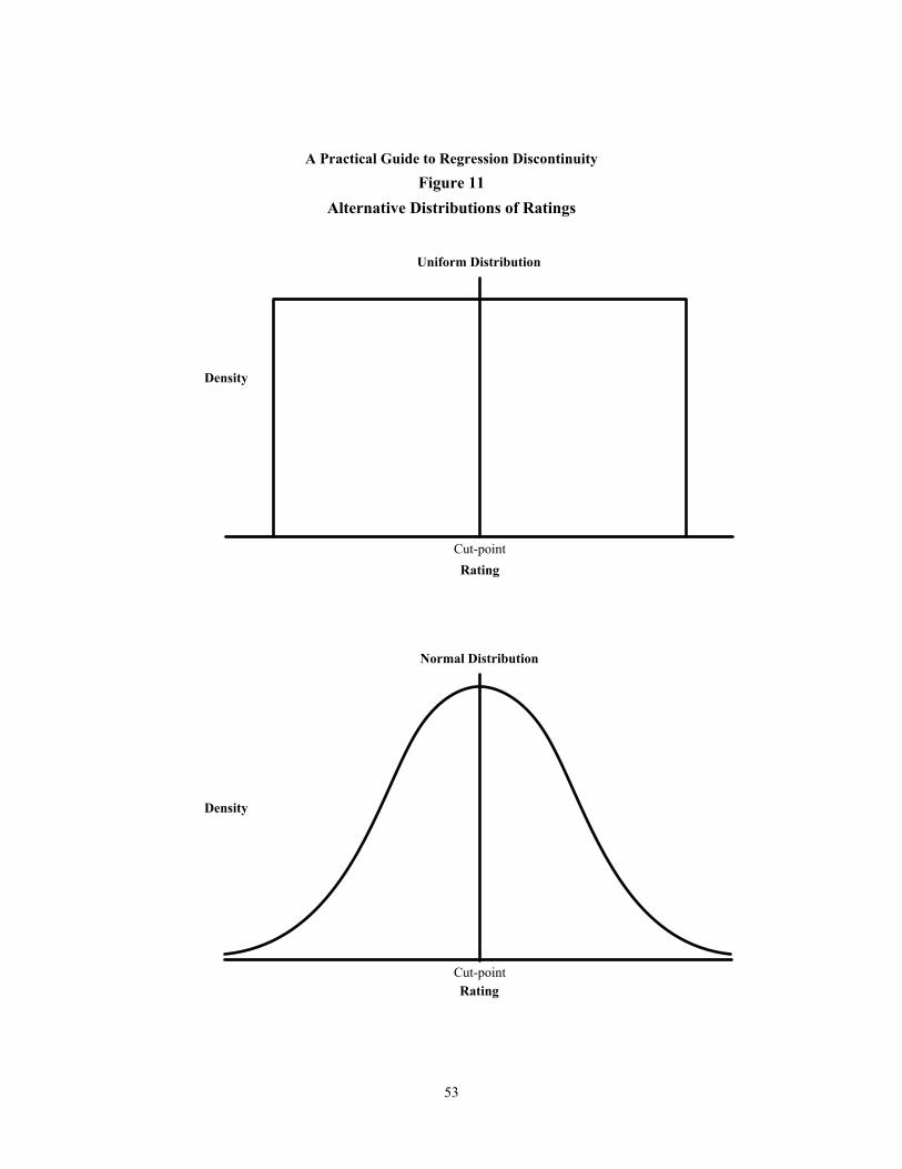
Density
Rating
Density
Rating
Normal Distribution
Uniform Distribution
Cut-point
Cut-point
A Practical Guide to Regression DiscontinuityFigure 11
Alternative Distributions of Ratings
53
Substituting these values into Equation 3 indicates that the MDE or MDES for an RD design with a balanced uniform distribution of ratings is twice that for an otherwise compa-rable randomized trial. This multiple is 1.66 for a balanced normal distribution of ratings.
By rearranging Equation 3, we can also obtain an expression for the “sample size mul-tiple” required for an RD design to produce the same MDE or MDES as an otherwise compara-ble randomized trial:
= (4) This expression, often referred to as the design effect, indicates that an RD sample with
a balanced uniform distribution of ratings must be ( . ), or four times the size of an otherwise
comparable randomized trial. The multiple is ( . ), or 2.75, for a balanced normal distribu-
tion of ratings.45 46
Table 6 presents collinearity coefficients and sample size multiples for several RD models and distributions of ratings. The table looks at three distributions: (1) the uniform distri-bution, (2) the standard normal distribution, and (3) the distribution of ratings (pretest scores) in the example RD data set. The latter distribution is included in order to look at some “real world” values for the relevant parameters (as seen in Figure 12, the distribution of ratings is approxi-mately normal but slightly skewed). The first set of columns in Table 6 is for a balanced distri-bution of units across either side of the cut-point (P = 0.50), while the second set of columns is for an unbalanced distribution with a third of the sample above the cut-point and two-thirds be-low the cut-point (P = 0.33).47 The top panel of the table reports the collinearity coefficient ( ) for each situation, and the bottom panel reports the corresponding sample size multiple (the de-sign effect) for an RD design relative to an otherwise comparable randomized trial. Each row in the table represents a different parametric RD model or functional form. Findings in the table indicate that:
45Goldberger (1972, 2008) proved this finding for a balanced normal distribution of ratings. 46This assumes a global and parametric approach to estimation. 47For symmetric distributions (standard normal and uniform), the collinearity coefficient is the same re-
gardless of whether the treatment is given to a third of the observations (P = 0.33) or to two-thirds of the obser-vations (P = 0.67). For an empirical distribution (like the example RD data set), the distribution of ratings is not symmetrical, so this equivalence does not hold. The results for the example data set in Table 6 are based on a 1:2 ratio of treatment to control (P = 33%). However, because the distribution of ratings is almost symmetrical, the results for a 2:1 ratio (P = 66%) are similar.
54
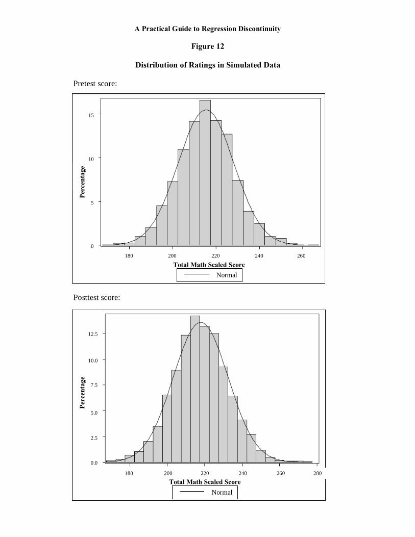
A Practical Guide to Regression Discontinuity
Figure 12
Distribution of Ratings in Simulated Data
Pretest score:
Posttest score:
Total Math Scaled Score
Total Math Scaled Score
180 200 220 240 260
180 200 220 240 260 280
15
10
5
0
Pe
rcen
tage
12.5
10.0
7.5
5.0
2.5
0.0
Perc
enta
ge
Normal
Normal
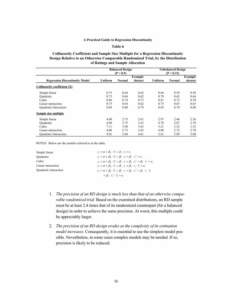
1. The precision of an RD design is much less than that of an otherwise compa-rable randomized trial. Based on the examined distributions, an RD sample must be at least 2.4 times that of its randomized counterpart (for a balanced design) in order to achieve the same precision. At worst, this multiple could be appreciably larger.
2. The precision of an RD design erodes as the complexity of its estimation model increases. Consequently, it is essential to use the simplest model pos-sible. Nevertheless, in some cases complex models may be needed. If so, precision is likely to be reduced.
Example ExampleUniform Normal dataset Uniform Normal dataset
0.75 0.64 0.62 0.66 0.59 0.580.75 0.64 0.62 0.79 0.65 0.640.86 0.74 0.73 0.81 0.72 0.700.75 0.64 0.62 0.75 0.63 0.630.89 0.80 0.79 0.83 0.74 0.80
Sample size multiple
4.00 2.75 2.61 2.97 2.46 2.364.00 2.75 2.63 4.78 2.87 2.787.11 3.90 3.65 5.21 3.52 3.324.00 2.75 2.65 4.00 2.72 2.709.01 5.04 4.81 5.81 3.89 5.00
Simple linear QuadraticCubicLinear interactionQuadratic interaction
Cubic
Quadratic InteractionLinear interactionCubicQuadraticSimple linear
Quadratic InteractionLinear interaction
A Practical Guide to Regression Discontinuity
Collinearity Coefficient and Sample Size Multiple for a Regression DiscontinuityDesign Relative to an Otherwise Comparable Randomized Trial, by the Distribution
of Ratings and Sample Allocation
QuadraticSimple linear
Regression Discontinuity Model
(P = 0.5) (P = 0.33)Balanced Design Unbalanced Design
Table 6
Collinearity coefficient (X)
NOTES: Below are the models referred to in the table.
iii
iiiiii
iiiiii
iiiiii
iiiii
iiii
Tr
TrrrTy
TrrTy
rrrTy
rrTy
rTy
εβββββα
εβββαεββββα
εβββαεββα
+⋅⋅+
⋅⋅+⋅+⋅+⋅+=
+⋅⋅+⋅+⋅+=+⋅+⋅+⋅+⋅+=
+⋅+⋅+⋅+=
+⋅+⋅+=
24
32
210
210
33
2210
2210
10
56

The precision of an RD design depends on the distribution of ratings around the cut-point.48 Because of the flexibility and variety in implementation of nonparametric statistical methods for RD analyses, it is not clear how to summarize the precision of such methods. What is clear, however, is that because they rely mainly, and often solely, on observations very near the cut-point (ignoring or greatly down-weighting all other observations), nonparametric meth-ods are far less precise than parametric methods for a given study sample.
48Schochet (2008) illustrates this point.
57
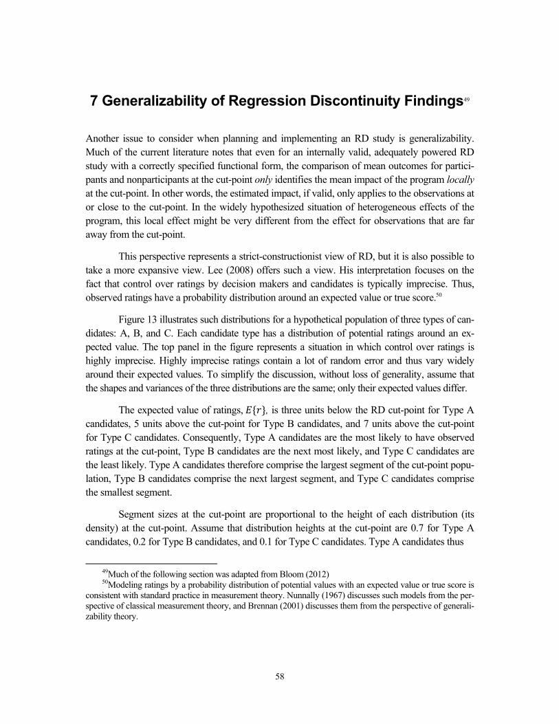
7 Generalizability of Regression Discontinuity Findings49
Another issue to consider when planning and implementing an RD study is generalizability. Much of the current literature notes that even for an internally valid, adequately powered RD study with a correctly specified functional form, the comparison of mean outcomes for partici-pants and nonparticipants at the cut-point only identifies the mean impact of the program locally at the cut-point. In other words, the estimated impact, if valid, only applies to the observations at or close to the cut-point. In the widely hypothesized situation of heterogeneous effects of the program, this local effect might be very different from the effect for observations that are far away from the cut-point.
This perspective represents a strict-constructionist view of RD, but it is also possible to take a more expansive view. Lee (2008) offers such a view. His interpretation focuses on the fact that control over ratings by decision makers and candidates is typically imprecise. Thus, observed ratings have a probability distribution around an expected value or true score.50
Figure 13 illustrates such distributions for a hypothetical population of three types of can-didates: A, B, and C. Each candidate type has a distribution of potential ratings around an ex-pected value. The top panel in the figure represents a situation in which control over ratings is highly imprecise. Highly imprecise ratings contain a lot of random error and thus vary widely around their expected values. To simplify the discussion, without loss of generality, assume that the shapes and variances of the three distributions are the same; only their expected values differ.
The expected value of ratings, { }, is three units below the RD cut-point for Type A candidates, 5 units above the cut-point for Type B candidates, and 7 units above the cut-point for Type C candidates. Consequently, Type A candidates are the most likely to have observed ratings at the cut-point, Type B candidates are the next most likely, and Type C candidates are the least likely. Type A candidates therefore comprise the largest segment of the cut-point popu-lation, Type B candidates comprise the next largest segment, and Type C candidates comprise the smallest segment.
Segment sizes at the cut-point are proportional to the height of each distribution (its density) at the cut-point. Assume that distribution heights at the cut-point are 0.7 for Type A candidates, 0.2 for Type B candidates, and 0.1 for Type C candidates. Type A candidates thus
49Much of the following section was adapted from Bloom (2012) 50Modeling ratings by a probability distribution of potential values with an expected value or true score is
consistent with standard practice in measurement theory. Nunnally (1967) discusses such models from the per-spective of classical measurement theory, and Brennan (2001) discusses them from the perspective of generali-zability theory.
58
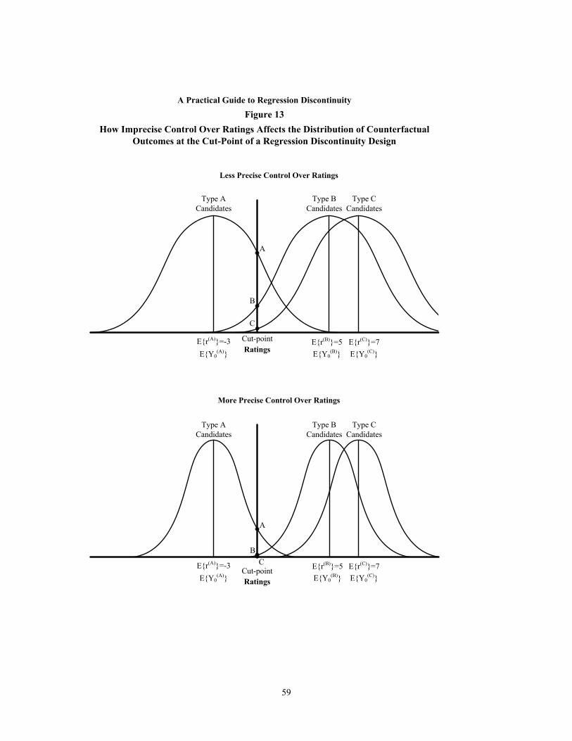
Ratings
Less Precise Control Over Ratings
Cut-pointE{r(A)}=-3E{Y0
(A)} E{Y0(B)} E{Y0
(C)}E{r(B)}=5 E{r(C)}=7
Ratings
More Precise Control Over Ratings
Cut-pointE{r(A)}=-3E{Y0
(A)} E{Y0(B)} E{Y0
(C)}E{r(B)}=5 E{r(C)}=7
BC
A
A
B
C
Type ACandidates
Type BCandidates
Type CCandidates
Type ACandidates
Type BCandidates
Type CCandidates
A Practical Guide to Regression DiscontinuityFigure 13
How Imprecise Control Over Ratings Affects the Distribution of Counterfactual Outcomes at the Cut-Point of a Regression Discontinuity Design
59
comprise .. . . , or0.70, of the cut-point population, Type B students comprise .. . . ,
or 0.20, and Type C candidates comprise .. . . , or 0.10. The cut-point population is thus somewhat heterogeneous in terms of expected ratings ( ( ) , ( ) and ( ) ). To the extent that expected ratings correlate with expected counterfactual outcomes ( ( ) , ( ) and { ( )}), the cut-point population also is somewhat heterogeneous in terms of expected counterfactual outcomes.51
The bottom panel in Figure 13 illustrates a situation with more precise control over rat-ings, which implies narrower distributions of potential values. Type C candidates, whose ex-pected rating is furthest from the cut-point, are extremely unlikely to have observed ratings at the cut-point. Because of this, they represent a very small proportion of the cut-point population. Type B candidates also represent a very small proportion of the cut-point population, but one that is larger than that for Type C candidates. The cut-point population thus is comprised almost exclusively of Type A candidates, which makes it quite homogeneous.
Several important implications flow from Lee’s insight about the generalizability of RD results. First, when ratings contain random error (which is probably most of the time), the popu-lation of candidates at a cut-point is not necessarily homogenous with respect to their true scores on the rating score. Second, other things being equal, the more random error that observed rat-ings contain, the more heterogeneous the cut-point population will be, and, therefore, the more broadly generalizable RD findings will be. Third, in the extreme, if ratings are assigned ran-domly, then the full range of candidate types will be assigned randomly above and below the cut-point. This case is equivalent to a randomized trial, and the resulting cut-point population will comprise the full target population. Current work in progress by Bloom and Porter takes this argument even further.
51The mean expected counterfactual outcome for the cut-point population is an average of the expected
value for each type of candidate weighted by the proportion of the cut-point population each type comprises.
60

8 Sharp and Fuzzy Designs52
Up to this point, we have focused exclusively on “sharp,” designs, where the rating variable per-fectly predicts treatment status. In other words, we have been focusing on cases in which the probability of treatment jumps from 0 to 1 at the cut-point. However, as already discussed, in many evaluation settings, treatment status is only partially determined by the rating variable and the predetermined cut-point, so that the probability of receiving treatment changes by less than a value of one as the rating crosses its cut-point value. These are referred to as fuzzy designs. Fol-lowing the lead of Battistin and Retorre (2008), one can distinguish three types of RD designs:
1. Sharp designs, as defined conventionally.
2. Type I fuzzy designs, in which some treatment group members do not re-ceive treatment. Such members are referred to as “no-shows.”53
3. Type II fuzzy designs, in which some treatment group members do not re-ceive treatment (no-shows), and some comparison group members do. (Members in the latter category are referred to as “crossovers.”)54
Figure 14 illustrates the key distinctions that exist among the three RD designs just de-scribed. The top graph in Figure 14 illustrates a sharp RD design, in which the probability of receiving treatment is equal to zero for schools with ratings below the cut-point and is equal to one for schools with ratings above the cut-point. Hence, the limiting value of the probability as the rating approaches the cut-point from below ( ) is zero, and its limiting value as the rating approaches the cut-point from above ( ) is one.55 The discontinuity in the probability at the cut-point ( − ) therefore equals one for a sharp RD.
The middle graph in Figure14 shows a Type I fuzzy design. The probability of receiv-ing the treatment is equal to zero for schools with ratings below the cut-point, but is only equal to 0.8 for schools with ratings above the cut-point, because some schools, for whatever reason, did not “take up” the treatment (that is, they were no-shows).
Finally, the bottom graph in Figure 14 shows a Type II fuzzy design, in which the prob-ability of receiving the treatment is equal to 0.015 for schools with ratings below the cut-point because there were some “crossovers,” and the probability of receiving the treatment for schools with ratings above the cut-point is equal to 0.8 for schools with ratings above the cut-point be-cause there were some “no-shows.”
52Much of the following section was adapted from Bloom (2012). 53Bloom (1984). 54Bloom et al. (1997). 55T is used to represent the probability of receiving treatment because it equals the mean value of T.
61
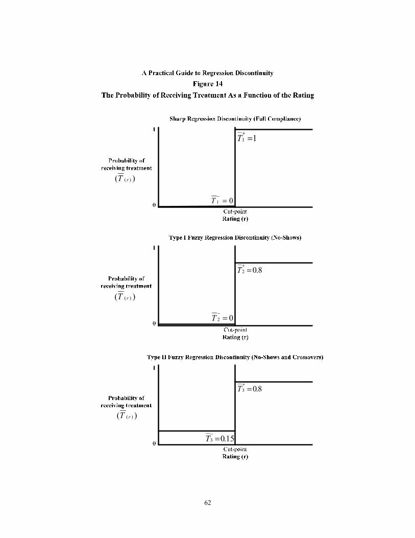
)( )( rT
)( )( rT
)( )( rT
11 =+
T
01 =−
T
02 =−
T
15.03 =−
T
8.02 =+
T
8.03 =+
T
62

Figure 15 illustrates how RD analysis can identify a treatment effect for the three de-signs. The top graph represents a sharp RD design, the middle graph represents a Type I fuzzy RD design, and the bottom graph represents a Type II fuzzy RD design. To make the example concrete, assume that candidates are schools, the outcome for each school is average student test scores, and the rating for each school is a measure of its student poverty (for example, the per-centage of students eligible for subsidized meals). Also assume that the analysis represents a population, not just a sample.
Curves in the graph are regression models of the relationship between expected out-comes ( ( )) and ratings (r).56 These curves are downward-sloping to represent the negative relationship that typically exists between student performance and poverty. Schools with ratings at or above a cut-point ( ∗) are assigned to treatment (for example, government assistance), and others are assigned to a control group that is not eligible for the treatment. In the top graph, all schools assigned to treatment receive it, and no schools assigned to control status receive it. In the middle graph, some schools assigned to treatment do not receive it, but no schools assigned to control status do receive it. In the bottom graph, some schools assigned to treatment do not receive it, and some schools assigned to control status do receive it.
For each graph, the solid line segment to the left of the cut-point indicates that expected outcomes for the control group decline continuously as ratings approach the cut-point from below — that is, as ratings increase toward their cut-point value. The symbol represents the expected outcome at the cut-point approached by this line. The dashed extension of the control group line segment represents what expected outcomes would be without treatment for schools with ratings above the cut-point (their expected counterfactual outcomes). The two line segments for the con-trol group form a continuous line through the cut-point; there is no discontinuity.
The solid line segment to the right of the cut-point indicates that expected outcomes for the treatment group rise continuously as ratings approach the cut-point from above — that is, as ratings decrease toward their cut-point value. The symbol represents the expected outcome at the cut-point approached by this line. The dashed extension of the treatment-group line seg-ment represents what outcomes would be for subjects with ratings below the cut-point if they had received treatment. The two line segments for the treatment group form a continuous line through the cut-point; again, there is no discontinuity.
When expected outcomes are a continuous function of ratings through the cut-point in the absence of treatment, the discontinuity, or gap, that exists between the solid line segment for the treatment group and the solid line segment for the control group, representing observable
56A regression model represents the relationship between expected values of a dependent variable and
specific values of an independent variable.
63
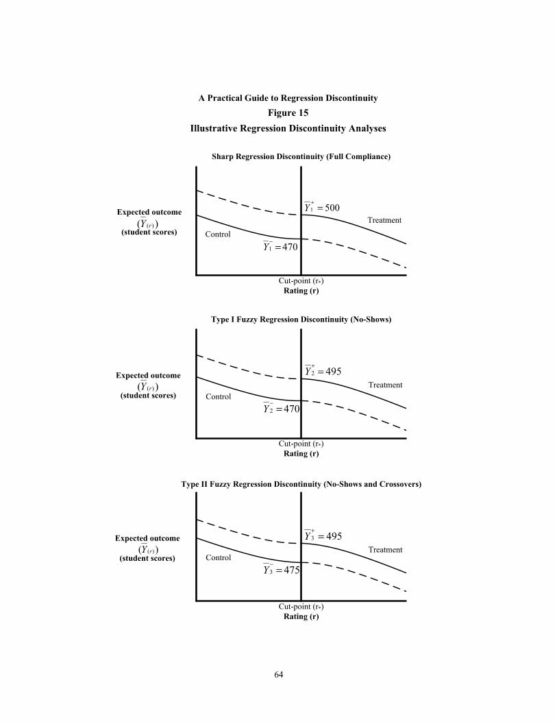
Expected outcome
(student scores)
Sharp Regression Discontinuity (Full Compliance)
Type I Fuzzy Regression Discontinuity (No-Shows)
Type II Fuzzy Regression Discontinuity (No-Shows and Crossovers)
Cut-point (r*)Rating (r)
Cut-point (r*)Rating (r)
Cut-point (r*)Rating (r)
)( )(rY
Expected outcome
(student scores) )( )(rY
5001 =+
Y
4701 =−
Y
Treatment
4952 =+
Y
4702 =−
Y
4953 =+
Y
4753 =−
Y
Treatment
Treatment
Control
Control
Control
A Practical Guide to Regression DiscontinuityFigure 15
Illustrative Regression Discontinuity Analyses
Expected outcome
(student scores) )( )(rY
64
comes for each group, can be attributed to the availability of treatment for treatment group members. This discontinuity ( − ) equals the average effect of assignment to treatment, which is often called the average effect of intent to treat (ITT). For an RD analysis, this is the average effect of intent to treat at the cut-point (ITTC).
Results in the top graphs of Figures 14 and 15 come together as follows. Moving from left to right, the probability of receiving treatment has a constant value of zero until the cut-point is reached, and the probability shifts abruptly to a constant value of one. If outcomes vary con-tinuously with ratings in the absence of treatment, then the only possible cause of a shift in ob-served outcomes at the cut-point (Figure 15) is the shift in the probability of receiving treatment (Figure 14).
Another way to explain this result is to note that as one approaches the cut-point, the re-sulting treatment group and control group become increasingly similar in all ways except for receipt of treatment. Hence, at the cut-point, assignment to treatment by ratings is like random assignment to treatment, as noted earlier. Differences at the cut-point between expected treat-ment group and control group outcomes, therefore, must be caused by the difference in treat-ment receipt.
A similar analysis can be conducted for the Type I and Type II Fuzzy designs. In these analyses, the effect of the treatment is diluted somewhat by the fact that not all schools with rat-ings above the cut-point actually received the treatment (the Type I Fuzzy design shown in the middle graph), and some of the schools with ratings below the cut-point did receive the treat-ment (the Type II Fuzzy designs shown in the bottom graph). This is reflected by the fact that the value of in the middle and bottom graphs is equal to 495 instead of 500, and the value of
is equal to 475 instead of 470 in the bottom graph. Thus, the discontinuity ( − ), which represents the average effect of assignment to treatment at the cut-point (ITTC), is small-er than in the case of the sharp design.
Estimation in the Context of a Fuzzy RD Design The graphs and prior discussion all focus on obtaining intent-to-treat estimates — that is, the average impact for those who were offered the treatment, whether or not they actually partici-pated in the treatment. Researchers are also often interested in obtaining unbiased estimates of the impact of the program on individuals who actually participated in the treatment.
As already noted, in the case of a fuzzy design, the observations on one side of the cut-point consist of individuals who were assigned to and received the treatment and also those who were assigned to the treatment but chose not to “take up” the treatment, while the observations on the other side of the cut-point consist of those who were assigned to the control condition
65

and thus did not receive treatment and those who were assigned to control condition and re-ceived the treatment anyway. Comparing these different types of units has only a limited causal interpretation.
It has been suggested that the treatment effect can be recovered by dividing the jump in the outcome-rating relationship by the jump in the relationship between treatment status and rat-ing. This will provide an unbiased estimate of the local average treatment effect (LATE), which is the impact of the program on the group of individuals who were assigned to the treatment and ac-tually participated in the treatment and those who were assigned to the control group and did not participate in the treatment (often called compliers).57 Analytically, the estimation of the treatment effect in a fuzzy RD design is often carried out by the two-stage least squares (2SLS) method. The following models illustrate how 2SLS analysis is carried out in this setting:
First-stage equation: = + + ( ) +
Second-stage equation: = + + ( )+
where:
= outcome for individual i;
= 1 if individual i receives the treatment, and 0 otherwise;
= 1 if individual i is assigned to treatment based on the cut-point rule, and 0 oth-erwise;
= rating for individual i; ( )= the relationship between the rating and treatment receipt for individual i; ( )= the relationship between the rating and outcome for individual i; and
= random error in first stage regression, assumed to be identically and inde-pendently distributed; and
= random error in first stage regression, assumed to be identically and inde-pendently distributed.
Ordinarily, the first-stage equation in this model is estimated using ordinary least
squares (OLS) regression. Then the predicted value of the mediator, , from the first-stage re-
57In the case of heterogeneous treatment effects (that is, where the effect of the treatment varies depending on who is treated) one cannot recover the treatment-on-the-treated (TOT) effect. The TOT effect is the impact of the treatment on all individuals who participated in the treatment regardless, of whether or not they were assigned to the treatment or not.
66
gression is used in place of in the second-stage equation, and this equation is estimated using OLS, which in turn produces an estimate of . Standard errors in the second-stage regression are adjusted to account for uncertainty in the first stage.
Similar to the sharp RD design, in the fuzzy setting, extra steps need to be taken to en-sure that the functional forms in both stages ( ( ) and ( ) ) are correctly speci-fied/estimated. As in the sharp RD setting, one can use either parametric or nonparametric ap-proaches to achieve this goal.
The parametric approach involves trying out polynomial functions of different orders and picking the model that fits the data the best. One can imagine that the functional forms in the two regressions differ. However, in order to use the 2SLS method and use the 2SLS stand-ard errors, the same functional form is often used for both regressions in practice.
The nonparametric approach involves picking the optimal bandwidth within which the functional form between rating and the outcome of interest can be approximated with a linear function. For the estimation in a fuzzy RD design, the literature recommends that the same bandwidth be used in both the first- and second-stage regressions (Imbens and Lemieux, 2008) for simplicity purposes. One can well imagine that the optimal bandwidth for the first-stage re-gression could be wider than the one for the second-stage regression, and using a wider band-width for first-stage regression might be desirable for efficiency reasons. However, if two dif-ferent bandwidths are used for these two regressions, then the first-stage and second-stage re-gressions will be estimated based on different samples, which will greatly complicate the com-putation of standard errors for the estimates. Furthermore, it will greatly increase the number of potential sensitivity checks that one has to conduct with different bandwidth choices, since, in-stead of one, two bandwidths, as well as their combinations, have to be changed simultaneously.
Precision in the Context of Fuzzy RD In addition to estimation, it is also important to consider the precision of a fuzzy RD design. The precision of a fuzzy RD design is often even less than that of the sharp design. Recall from sec-tion 6 that the “sample size multiple” required for an RD design to produce the same MDE or MDES as an otherwise comparable randomized trial can be expressed as the following:
= where is the proportion of variation in treatment status (T) that is predicted by the centered rating variable and any other variables included in the regression. This expression is also re-ferred to as the design effect of a sharp RD design.
67
As derived by Schochet (2008), the design effect for the fuzzy RD design, relative to a comparable randomized trial with 100 percent compliance is:
= 1(1 − 2)( − )2
where: = the participation rate (1-“no-show” rate) of those assigned to the treatment group at
the cut-point;
= the “crossover” rate of those assigned to the control group at the cut-point; and
is defined as before.
In other words, relative to a comparable randomized trial with 100 percent compliance
(that is, no “no-shows” and no “crossovers”), the design effect of a fuzzy RD design depends on (1) the proportion of variation in T that is predicted by the rating and other covariates; and (2) the compliance rate (1-“no-show” rate — “crossover” rate) at the cut-point. Compared with equation 4 in section 6, the higher the compliance rate at cut-point is (or the less fuzzy it is), the closer the design effect for fuzzy RD is to the one for sharp RD, holding everything else con-stant.
When − (the difference in treatment receipt rates between the treatment and con-trol group members in the full sample) is equal to − (the difference in treatment receipt rates between treatment and control group members around the cut-off), then the ratio between the two reduces to one, and the design effect is equivalent to that for a sharp design. This is the situation depicted in Figure 14. In the third panel of that figure, the probability of receiving treatment is less than 1 if assigned to the treatment group and greater than 0 if assigned to the control group, but on either side of the cut-point the probability of receiving treatment remains constant for every value of the rating variable.
However, if the probability of being a “no-show” or a “crossover” increases as you get closer to the cut-point — for example, if a teacher has a group of students who are eligible to receive a treatment based on test scores, but she decides to treat the neediest of the eligible stu-dents first (those with the lowest test scores) and runs out of time to treat those who are less needy (those with higher test scores) ― then the ratio of − to − will be greater than 1, and the design effect will be increased proportionally. Similarly, if the parents of the neediest students who just missed the cut-off aggressively seek out treatment for their students, but those with the highest test scores, who were furthest from the cut-point, do not, there will be more
68
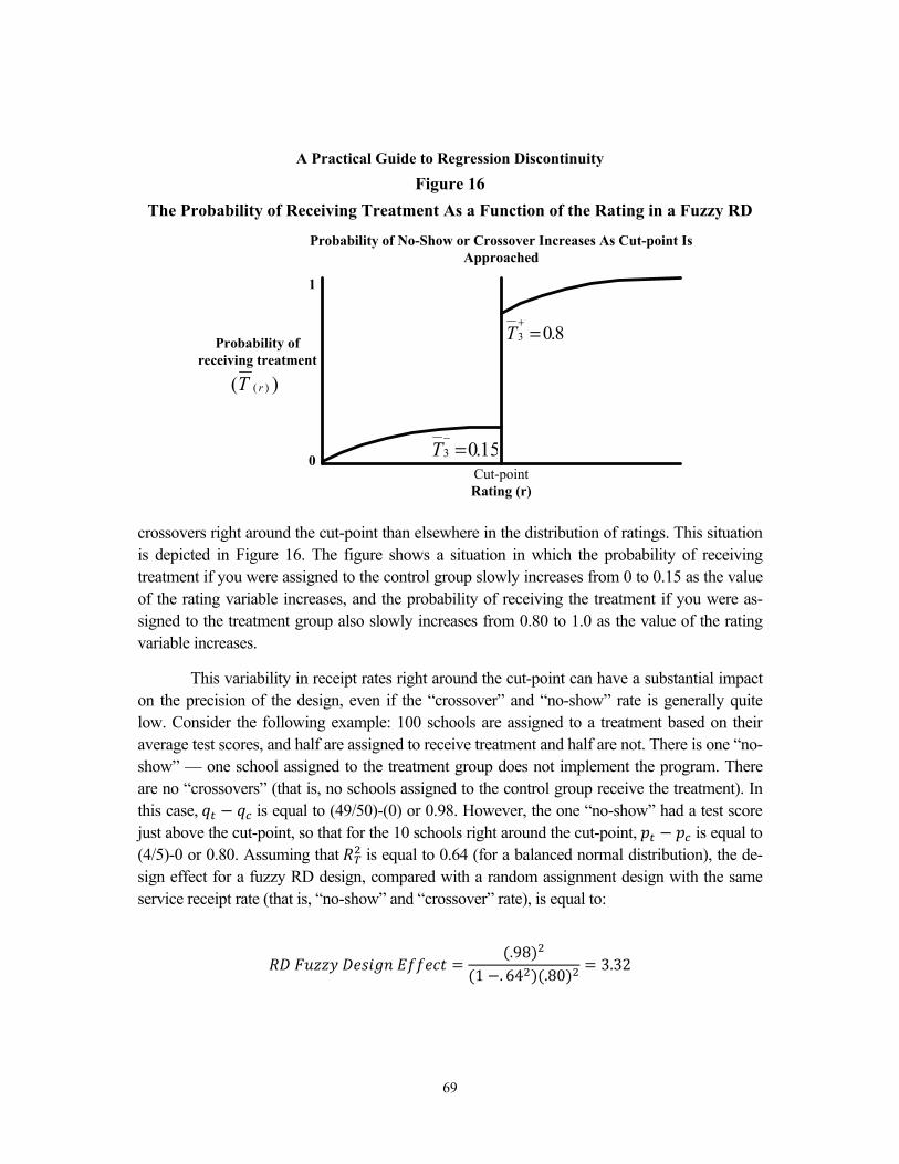
crossovers right around the cut-point than elsewhere in the distribution of ratings. This situation is depicted in Figure 16. The figure shows a situation in which the probability of receiving treatment if you were assigned to the control group slowly increases from 0 to 0.15 as the value of the rating variable increases, and the probability of receiving the treatment if you were as-signed to the treatment group also slowly increases from 0.80 to 1.0 as the value of the rating variable increases.
This variability in receipt rates right around the cut-point can have a substantial impact on the precision of the design, even if the “crossover” and “no-show” rate is generally quite low. Consider the following example: 100 schools are assigned to a treatment based on their average test scores, and half are assigned to receive treatment and half are not. There is one “no-show” — one school assigned to the treatment group does not implement the program. There are no “crossovers” (that is, no schools assigned to the control group receive the treatment). In this case, − is equal to (49/50)-(0) or 0.98. However, the one “no-show” had a test score just above the cut-point, so that for the 10 schools right around the cut-point, − is equal to (4/5)-0 or 0.80. Assuming that is equal to 0.64 (for a balanced normal distribution), the de-sign effect for a fuzzy RD design, compared with a random assignment design with the same service receipt rate (that is, “no-show” and “crossover” rate), is equal to:
= (.98)(1 −. 64 )(.80) = 3.32
Probability of No-Show or Crossover Increases As Cut-point Is Approached
)( )( rT
1
0 15.03 =−
T
8.03 =+
T
A Practical Guide to Regression DiscontinuityFigure 16
The Probability of Receiving Treatment As a Function of the Rating in a Fuzzy RD
Cut-pointRating (r)
Probability of receiving treatment
69

At the same time, if the service receipt rate around the cut-off in the RD design is the same as the receipt rate for the full study sample, the design effect would be only 2.78 (the same design effect as for the sharp RD design compared with a random assignment study with no “no-shows” or “crossovers”). Since the treatment effects for an RD design are marginal treat-ment effects, it is the “no-show” and “crossover” rate right around the cut-off that matters. If the receipt rate around the cut-off is equal to the receipt rate for the whole study population, howev-er, there is no additional loss of power compared with a random assignment study with a com-parable service receipt rate.
70

9 Concluding Thoughts
As stated at this beginning of this guide, this document is intended to provide practical guidance to researchers who are considering using an RD design to estimate treatment effects for an in-tervention. The guide provides an overview of the key issues, procedures, and challenges related to (1) graphical analysis, (2) parametric and nonparametric estimation, (3) assessing the internal validity of the design, (4) determining the precision of the design, (5) assessing the generaliza-bility of the results, and (6) issues to consider when faced with a fuzzy rather than sharp RD design. The order of presentation of these topics in this guide was chosen to facilitate the presentation of methods. It does not reflect the order in which these topics should necessarily be addressed by researchers considering an RD design. The order in which these issues are ad-dressed will depend, in part, on whether the researcher is conducting a prospective or retrospec-tive study. A prospective study is one in which the researcher will be working with the organi-zation or group that is implementing the intervention to assign treatment to individuals in a way that is consistent with an RD design. A retrospective study is one in which the researcher will use existing data that lend themselves to RD analysis to assess the impact of a program. Since retrospective designs are more common, we first outline the steps that researchers should take in implementing such a design. We then outline the steps researchers conducting a prospective study should take.
We recommend that researchers conducting a retrospective RD analysis proceed as fol-lows:
1. Determine whether or not you have a valid RD design.
i. Gather all relevant information regarding the process for assigning the ratings and determining the cut-point.
ii. If the design appears to be valid based on the process used to assign ratings and determine the cut-point, conduct graphical and empirical analyses to further confirm that the design is valid.
2. Assess whether or not the design is sharp or fuzzy, by conducing graphical analyses in which you plot the probability of receiving treatment as a func-tion of the rating.
3. Assess the degree of precision you have for detecting impacts. If you have a fuzzy design, take this into account when assessing precision.
4. Once you have determined that you have a valid design with sufficient power to detect effects, proceed with analysis.
71

i. Begin by graphing the outcome versus the rating variable, using the techniques described here to smooth the plot. Visually inspect the graph to assess whether or not there is a discontinuity at the cut-point.
ii. If you are using a large data set, with more than sufficient power to detect effects, begin with a nonparametric estimation approach that limits the bandwidth of your estimation. Conduct sensitivity analyses using a parametric approach.
iii. If you have a relatively small data set, with more limited power to detect effects, begin with a parametric estimation approach. Conduct nonparametric analyses as sensitivity tests.
iv. If you have a fuzzy design, take this into account when conducting analyses.
v. Unless evidence strongly suggests otherwise, use the simplest model possible to conduct analyses. Use more complex models as sensitivi-ty checks only.
5. Assess the generalizability of your findings. Consider how much random er-ror the ratings contain. This will provide some insight into how heterogene-ous the sample around the cut-point is likely to be. The greater the degree of random error, the more broadly generalizable the findings will be.
For researchers conducting a prospective study, we recommend proceeding as follows:
1. Determine the sample size you will need to detect effects. Take into account the fact that there may be “no-shows” or “crossovers” and that this will affect the precision of your estimates.
2. Work with implementers to ensure that the assignment to treatment status will result in a valid design
3. Monitor the implementation of the design to ensure compliance and mini-mize “no-shows” and “crossovers” and also to make sure that instances of noncompliance are properly identified so that they can be accounted for later in your analysis.
4. When the evaluation is complete, assess the validity of the design, using graphical and empirical techniques.
72

5. Determine whether the design is fuzzy or sharp.
6. Proceed with analyses, following the procedures outlined in step 4 above.
7. Assess the generalizability of your findings.
Following these steps will help to ensure that the results of the RD analysis are robust and can be well defended.
73

Appendix A
Glossary


Akaike information criterion (AIC): A measure of the relative goodness of fit of a statistical model. Conceptually, it describes the trade-off between bias and variance in model construction and offers a relative measure of the information lost when a given model is used to describe reality. Bandwidth: In local linear regression with a rectangular kernel, the range of points on each side of the cut-off that will be included in the regression.
Bin: A bin divides the distribution of ratings into equal-size intervals for graphical or other analyses. Also called bin width.
Bin width: The width of the bin on the rating scale. Also called bin size.
Crossover: When some comparison group members receive treatment.
Cross-validation: A method used to find the optimal bandwidth for graphical or other analyses.
Compliers: Individuals who receive the treatment when assigned to the treatment group and do not receive the treatment when assigned to the control group Cut-point: The point in the rating scale that determines whether or not a group or individu-al will be included in the treatment. Groups or individuals with ratings above (or below) the cut-point receive the treatment; those with ratings below (or above) the cut-point do not receive the treatment. Also called cut-off threshold or discontinuity point. Design effect: The “sample size multiple” required for a design, such as regression discon-tinuity, to produce the same MDE or MDES as an otherwise comparable randomized trial.
Exogenous: External to the design or study. An exogenous variable is not impacted by factors or variables within a study.
Functional form: The relationship between a dependent variable and an explanatory variable (or variables) expressed algebraically. The simplest functional form is a linear functional form, which is graphically represented by a straight line. Other functional forms include quadratic, cubic, and models with interaction terms.
Fuzzy RD design: When not all subjects receive their assigned treatment or control condition.
Intent to treat (ITT): The average impact for those who were offered the treatment, whether or not they actually participated in the treatment.
76

Intent to treat at the cut-point (ITTC): The average effect of assignment to treatment at the cut-point.
Local average treatment effect (LATE): The impact of the program on compliers (that is, individuals who receive the treatment when assigned to the treatment group and do not receive the treatment when assigned to the control group). Also called Complier average causal effect (CACE). Local linear regression: A local linear regression is estimated separately for each bin in a sample. The regression can be weighted (for example, using a kernel) or unweighted. For many regression discontinuity analyses, treatment effects are estimated from local linear regressions for the two bins adjacent to the cut-point.
Minimum detectable effect (MDE): The smallest treatment effect that a research design has an acceptable chance of detecting if it exists. Minimum detectable effects are reported in natural units, such as scale-score points for standardized tests. Minimum detectable effect size (MDES): A minimum detectable effect size is a mini-mum detectable effect divided by the standard deviation of the outcome measure. It is reported in units of standard deviations. Nonparametric estimation: An estimation technique that does not assume a particular functional form but rather constructs one according to information derived from the data.
No-show: When some treatment group members do not receive treatment.
Rating variable: A continuous variable measured before treatment, the value of which determines whether or not a group or individual is assigned to the treatment. Also called forcing variable, running variable, or assignment variable.
Regression discontinuity design: A method for estimating impacts in which candidates are selected for treatment based on whether their value for a numeric rating exceeds a designat-ed threshold or cut-point. Sharp RD design: When all subjects receive their assigned treatment or control condition.
Treatment on the treated (TOT): The impact of the program on individuals who actually participated in the treatment. Also called Average treatment effect on the treated (ATET).
Unbiased estimator: When the expected value of the parameter being estimated is equal to the true value of that parameter.
77

Appendix B
Checklists for Researchers


Checklist for Researchers Conducting a Retrospective RD Analysis
Determine whether or not you have a valid RD design (See section 5).
o Gather all relevant information regarding the process for assigning the ratings and determining the cut-point.
o If the design appears to be valid based on the process used to assign ratings and determine the cut-point, conduct graphical and empirical analyses to further confirm that the design is valid.
Assess whether or not the design is sharp or fuzzy by conducing graphical analyses in which you plot the probability of receiving treatment as a func-tion of the rating (See section 3 for a Guide to Graphical Analysis).
Assess the degree of precision you have for detecting impacts. If you have a fuzzy design, take this into account when assessing precision (See section 6 for Sharp Designs and section 8 for Fuzzy Designs).
Once you have determined that you have a valid design with sufficient power to detect effects proceed with analysis (See section 4).
o Begin by graphing the outcome versus the rating variable, using the techniques described in section 3 to smooth the plot. Visually inspect the graph to assess whether or not there is a discontinuity at the cut-point.
o If you are using a large data set, with more than sufficient power to detect effects, begin with a nonparametric estimation approach that limits the bandwidth of your estimation (See section 4). Conduct sen-sitivity analyses using a parametric approach.
o If you have a relatively small data set, with more limited power to de-tect effects, begin with a parametric estimation approach (See section 4). Conduct nonparametric analyses as sensitivity tests.
o If you have a fuzzy design, take this into account when conducting analyses (See section 8).
o Unless evidence strongly suggests otherwise, use the simplest model possible to conduct analyses. Use more complex models as sensitivity checks only.
80

Assess the generalizability of your findings. Consider how much random er-ror the ratings contain. This will provide some insight into how heterogene-ous the sample around the cut-point is likely to be. The greater the degree of random error, the more broadly generalizable the findings will be (See sec-tion 7).
Checklist for Researchers Conducting a Prospective
RD Study
Determine the sample size you will need to detect effects. Take into account the fact that there may be “no-shows” or “crossovers” and that this will affect the precision of your estimates (see section 4 and section 7).
Work with implementers to ensure that the assignment to treatment status will result in a valid design (see section 5).
Monitor the implementation of the design to ensure compliance and minimize “no-shows” and “crossovers” and also to make sure that instances of non-compliance are properly identified so that they can be accounted for later in your analysis.
When the evaluation is complete, assess the validity of the design using graphical and empirical techniques (see section 5).
Determine whether the design is fuzzy or sharp (see section 8 and section 3 for a Guide to Graphical Analyses).
Proceed with analyses (see section 4).
o Begin by graphing the outcome versus the rating variable, using the techniques described in section 3 to smooth the plot. Visually inspect the graph to assess whether or not there is a discontinuity at the cut-point.
o If you are using a large data set, with more than sufficient power to detect effects, begin with a nonparametric estimation approach that limits the bandwidth of your estimation (see section 4). Conduct sen-sitivity analyses using a parametric approach.
o If you have a relatively small data set, with more limited power to de-tect effects, begin with a parametric estimation approach (see section 4). Conduct nonparametric analyses as sensitivity tests.
81

o If you have a fuzzy design, take this into account when conducting analyses (see section 8).
o Unless evidence strongly suggests otherwise, use the simplest model possible to conduct analyses. Use more complex models as sensitivity checks only.
Assess the generalizability of your findings. Consider how much random er-ror the ratings contain. This will provide some insight into how heterogene-ous the sample around the cut-point is likely to be. The greater the degree of random error, the more broadly generalizable the findings will be (see section 7).
82

Appendix C
For Further Investigation


Note: The following is a list of suggested resources for individuals who are interested in learning more about regression discontinuity designs. It is a starting place and is in no way meant to be an exhaustive list.
Bloom, H. S. 2012. “Modern Regression Discontinuity Analysis.” Journal of Research on Educational Effectiveness 5 (1): 43-82.
Cook, T. D. 2008. “Waiting for Life to Arrive: A History of the Regression-Discontinuity design in Psychology, Statistics and Economics.” Journal of Economet-rics 142 (2): 636-654.
Gleason, P. M., A. M. Resch, and J. A. Berk. 2012. Replicating Experimental Impact Estimates Using a Regression Discontinuity Approach. NCEE Reference Report 2012-4025. Washington, DC: National Center for Education Evaluation and Regional Assis-tance, Institute of Education Sciences, U.S. Department of Education.
Lee, D. S., and D. Card. 2008. “Regression Discontinuity Inference with Specification Error. Journal of Econometrics 142 (2): 655-674.
Lee, D., and T. Lemieux. 2010. “Regression Discontinuity Designs in Economics.” Journal of Economic Literature 48: 281-355.
Imbens, G. W., and T. Lemieux. 2008. “Regression Discontinuity Designs: A Guide to Practice. Journal of Econometrics 142 (2): 615-635.
McCrary, J. 2008. “Manipulation of the Running Variable in the Regression Disconti-nuity Design: A Density Test.” Journal of Econometrics 142 (2): 698-714.
Schochet, P., T. Cook, J. Deke, G. Imbens, J. R. Lockwood, J. Porter, and J. Smith. 2010. Standards for Regression Discontinuity Designs. Retrieved from What Works Clearing-house Web site: http://ies.ed.gov/ncee/wwc/pdf/wwc_rd.pdf.
85

References
Angrist, J., and V. Lavy.1999. “Using Maimonides’ Rule to Estimate the Effect of Class Size on Student Achievement.” Quarterly Journal of Economics 114 (May): 535-575.
Battistin, E., and E. Retore. 2008. “Ineligibles and Eligible Non-Participants as a Dou-ble Comparison Group in Regression Discontinuity Designs.” Journal of Econometrics 142: 715-730.
Black, D., J. Galdo, and J. Smith. 2007. “Evaluating the Worker Profiling and Reemployment Services System Using a Regression Discontinuity Design.” Ameri-can Economic Review Papers and Proceedings 97 (2): 104-107. Bloom, H. S. 1984. “Accounting for No-Shows in Experimental Evaluation Designs.” Evaluation Review 8: 225-246.
Bloom, H. S. 1995. “Minimum Detectable Effects: A Simple Way to Report the Statistical Power of Experimental Designs.” Evaluation Review 19: 547-556.
Bloom, H. S. 2005. Learning More from Social Experiments: Evolving Analytic Ap-proaches. New York: Russell Sage.
Bloom, H. S. 2012. “Modern Regression Discontinuity Analysis.” Journal of Research on Educational Effectiveness 5 (1): 43-82.
Bloom, H. S., L. L. Orr, G. Cave, S. H. Bell, F. Doolittle, and W. Lin. 1997. “The Bene-fits and Costs of JTPA Programs: Key Findings from the National JTPA Study.” The Journal of Human Resources 32 (3): 549-576.
Bloom, H. S., C. J. Hill, A. R. Black, and M. W. Lipsey. 2008. “Performance Trajecto-ries and Performance Gaps as Achievement Effect-Size Benchmarks for Educational Interventions.” Journal of Research on Educational Effectiveness 1: 289-328.
Bloom, H. S., and K. Porter (in progress). Assessing the Generalizability of Estimates of Causal Effects from Regression Discontinuity Designs.
Bloom, H. S., L. Richburg-Hayes, and A. R. Black. 2007. “Using Covariates to Im-prove Precision for Studies That Randomize Schools to Evaluate Educational Interven-tions.” Educational Evaluation and Policy Analysis 29 (1): 30-59.
Blundell, R., and A. Duncan. 1998. “Kernel Regression in Empirical Microeconomics." The Journal of Human Resources 33 (1): 62-87.
Brennan, R. L. 2001. Generalizability Theory. New York: Springer.
87

Cohen, J. 1988. Statistical Power Analysis for the Behavioral Sciences (2nd ed.). Hills-dale, NJ: Lawrence Erlbaum Associates.
Cook, T. D. 2008. “Waiting for Life to Arrive: A History of the Regression-Discontinuity Design in Psychology, Statistics and Economics.” Journal of Economet-rics 142 (2): 636-654.
Cook, T. D., W. R. Shadish, and V. C. Wong. 2008. “Three Conditions Under Which Experiments and Observational Studies Produce Comparable Causal Estimates: New Findings from Within-Study Comparisons.” Journal of Policy Analysis and Manage-ment 27 (4): 724-750.
DesJardins, S. L., and B. P. McCall. 2008. The Impact of the Gates Millennium Schol-ars Program on the Retention, College Finance- and Work-Related Choices, and Fu-ture Educational Aspirations of Low-Income Minority Students (Working Paper). Re-trieved May 16, 2012, from http://www-personal.umich.edu/~bpmccall/Desjardins_McCall_GMS_June_2008.pdf.
DiNardo, J., and D. S. Lee. 2004. Economic Impacts of New Unionization on Private Sector Employers: 1984-2001.” Quarterly Journal of Economics 119 (4): 1383-1441.
Fan, J. 1992. “Design-Adaptive Non-Parametric Regression.” Journal of the American Statistical Association 87 (420): 998-1004.
Fan, J., and I. Gijbels. 1996. Local Polynomial Modeling and Its Applications. London: Chapman and Hall.
Gamse, B. C., H. S. Bloom, J. J. Kemple, and R. T. Jacob. 2008. Reading First Impact Study Final Report (NCEE 2009-4038). Washington, DC: National Center for Educa-tion Evaluation and Regional Assistance, Institute of Education Sciences, U.S. Depart-ment of Education.
Gleason, P. M., A. M. Resch, and J. A. Berk. 2012. Replicating Experimental Impact Estimates Using a Regression Discontinuity Approach. NCEE Reference Report 2012-4025. Washington, DC: National Center for Education Evaluation and Regional Assis-tance, Institute of Education Sciences, U.S. Department of Education.
Goldberger, A. S. 1972. “Selection Bias in Evaluating Treatment Effects: Some Formal Illustrations.” (Discussion Paper 129-72). Madison, WI: University of Wisconsin-Madison, Institute for Research on Poverty.
Goldberger, A. S. 2008. “Selection Bias in Evaluating Treatment Effects: Some Formal Illustrations.” Advances in Econometrics 21: 1-31.
88

Grissom, R. J., and J. J. Kim. 2005. Effect Sizes for Research: A Broad Practical Per-spective. Mahwah, NJ: Lawrence Erlbaum Associates.
Guggenberger, P., and G. Kumar. 2011. “On the Size Distortion of Tests After an Overidentifying Restrictions Pretest.” Journal of Applied Econometrics. DOI: 10.1002/jae 1251.
Hahn, J., P. Todd, and W. van de Klaauw. 1999. Evaluating the Effect of an Antidis-crimination Law Using a Regression-Discontinuity Design (NBER Working Paper 7131). Cambridge, MA: National Bureau of Economic Research.
Hahn, J., P. Todd, W. van de Klaauw. 2001. “Identification and Estimation of Treat-ment Effects with a Regression-Discontinuity Design. Econometrica 69 (1), 201-209.
Härdle, W., and O. Linton. 1994. “Applied Non-Parametric Methods.” Pages 2295-2339 in R. F. Engle and D. L. MacFadden (eds.), Handbook of Econometrics 4. Am-sterdam: North-Holland Publishing Co.
Heckman, J., and Robb, R. Jr. 1985. “Alternative Methods for Evaluating the Impact of Interventions: An Overview.” Journal of Econometrics 30 (1-2): 239-267.
Hill, C. J., H. S. Bloom, A. R Black, and M. Lipsey. 2008. “Empirical Benchmarks for Interpreting Effect Sizes in Research.” Child Development Perspectives 2 (3): 172-177.
Imbens, G. W., and K. Kalyanaraman. 2009. Optimal Bandwidth Choice for the Re-gression Discontinuity Estimator. (Unpublished working paper).
Imbens, G. W., and T. Lemieux. 2008. “Regression Discontinuity Designs: A Guide to Practice.” Journal of Econometrics 142 (2): 615-635.
Jacob, B. A., and L. Lefgren, L. 2006. “Remedial Education and Student Achievement: A Regression-Discontinuity Analysis.” The Review of Economics and Statistics 86 (1): 226-244.
Lee, D. S. 2008. “Randomized Experiments from Non-Random Selection in U.S. House Elections.” Journal of Econometrics 142 (2): 675-697.
Lee, D. S., and Card, D. 2008. “Regression Discontinuity Inference with Specification Error. Journal of Econometrics 142 (2): 655-674.
Lee, D., and T. Lemieux. 2010. “Regression Discontinuity Designs in Economics.” Journal of Economic Literature 48: 281-355.
Lemieux, T., and K. Milligan. 2004. Incentive Effects of Social Assistance: A Regres-sion Discontinuity Approach (NBER Working Paper 10541). Cambridge, MA: National Bureau of Economic Research.
89

Ludwig, J., and D. Miller. 2005. Does Head Start Improve Children’s Life Chances? Evidence from a Regression Discontinuity Design (NBER Working Paper 11702). Cambridge, MA: National Bureau of Economic Research.
McCrary, J. 2008. “Manipulation of the Running Variable in the Regression Disconti-nuity Design: A Density Test.” Journal of Econometrics 142 (2): 698-714.
McEwan, P. J., and J. S. Shapiro. 2008. “The Benefits of Delayed Primary School En-rollment: Discontinuity Estimates Using Exact Birth Dates.” Journal of Human Re-sources 43 (1): 1-29.
Nunnally, J. C. 1967. Psychometric Theory. New York: McGraw-Hill.
Orr, L. L. 1998. Social Experiments: Evaluating Public Programs with Experimental Methods. Thousand Oaks, CA: Sage.
Pagan, A., and A. Ullah. 1999. Nonparametric Econometrics. Cambridge, UK: Cambridge University Press. Porter, J. 2003. Estimation in the Regression Discontinuity Model (Working Paper). Cambridge, MA: Harvard University Department of Economics.
Rosenthal, R., R. L. Rosnow, and D. B. Rubin. 2000. Contrasts and Effect Sizes in Be-havioral Research: A Correlational Approach. Cambridge, UK: Cambridge University Press.
Schochet, P. Z. 2008. Technical Methods Report: Statistical Power for Regression Dis-continuity Designs in Education Evaluations (NCEE 2008-4026). Washington, DC: Na-tional Center for Education Evaluation and Regional Assistance, Institute of Education Sciences, U.S. Department of Education.
Shadish, W. R., T. D. Cook, and D. T. Campbell. 2002. Experimental and Non-Experimental Designs for Generalized Causal Inference. Boston: Houghton Mifflin.
Spybrook, J. K. 2007. Examining the Experimental Designs and Statistical Power of Group Randomized Trials Funded by the Institute of Education Sciences (Doctoral dis-sertation). Available from ProQuest Dissertations and Theses Database. (UMI No. AAT 3287637).
Thistlethwaite, D., and D. Campbell. 1960. “Regression-Discontinuity Analysis: An Al-ternative to the Ex Post Facto Experiment.” Journal of Educational Psychology 51: 309-317.
van der Klaauw, W. 1997. “A Regression-Discontinuity Evaluation of the Effect of Fi-nancial Aid Offers on College Enrollment.” Manuscript. New York: New York Univer-sity, Department of Economics.
90

van der Klaauw, W. 2002. “Estimating the Effect of Financial Aid Offers on College Enrollment: A Regression-Discontinuity Approach.” International Economic Review 43 (4): 1249-1287.
van der Klaauw, W. 2008. “Regression-Discontinuity Analysis: A Survey of Recent Developments in Economics.” Labour 22 (2): 219-245.
91

About MDRC
MDRC is a nonprofit, nonpartisan social and education policy research organization dedicated to learning what works to improve the well-being of low-income people. Through its research and the active communication of its findings, MDRC seeks to enhance the effectiveness of so-cial and education policies and programs.
Founded in 1974 and located in New York City and Oakland, California, MDRC is best known for mounting rigorous, large-scale, real-world tests of new and existing policies and programs. Its projects are a mix of demonstrations (field tests of promising new program approaches) and evaluations of ongoing government and community initiatives. MDRC’s staff bring an unusual combination of research and organizational experience to their work, providing expertise on the latest in qualitative and quantitative methods and on program design, development, implementa-tion, and management. MDRC seeks to learn not just whether a program is effective but also how and why the program’s effects occur. In addition, it tries to place each project’s findings in the broader context of related research — in order to build knowledge about what works across the social and education policy fields. MDRC’s findings, lessons, and best practices are proac-tively shared with a broad audience in the policy and practitioner community as well as with the general public and the media.
Over the years, MDRC has brought its unique approach to an ever-growing range of policy are-as and target populations. Once known primarily for evaluations of state welfare-to-work pro-grams, today MDRC is also studying public school reforms, employment programs for ex-offenders and people with disabilities, and programs to help low-income students succeed in college. MDRC’s projects are organized into five areas:
Promoting Family Well-Being and Children’s Development
Improving Public Education
Raising Academic Achievement and Persistence in College
Supporting Low-Wage Workers and Communities
Overcoming Barriers to Employment
Working in almost every state, all of the nation’s largest cities, and Canada and the United Kingdom, MDRC conducts its projects in partnership with national, state, and local govern-ments, public school systems, community organizations, and numerous private philanthropies.