Embed Size (px)
Citation preview

A PREDICTIVE SAFETY MANAGEMENT SYSTEM SOFTWARE
PACKAGE BASED ON THE CONTINUOUS HAZARD TRACKING
AND FAILURE PREDICTION METHODOLOGY
YEAR 1 FINAL REPORT
December 1, 2002 to November 30, 2003
November 30, 2003
Principal Investigator: Rolando Quintana, Ph.D., P.E.
The University of Texas at E1 Paso
Department of Mechanical and Industrial Engineering
500 West University Drive
E1 Paso, Texas 79968-0521
NASA Grant Number: NAG10-331
Technical POC: Mr. Bhupendra Deliwala, Kennedy Space Center
Mr. Chris Pino, OP-AM

Acknowledgements
The NASA Predictive Safety research team is very grateful to Mr. Bob Deliwala
for his support, guidance and vision on the paradigm of predictive safety engineering and
management. Many safety professionals have graduated with Bachelor's and Master's
degrees working as research assistants in the NASA Predictive Safety Laboratory,
including a significant number of women and underrepresented minorities. Through this
grant 3avier Avalos (M.S., Summer 2003) and Kene Roldan (M.S., Summer 2003) have
been supported. Mr. Chris Pino is also acknowledged for his support.
ii

Executive Summary
The goal of this research was to integrate a previously validated and reliable
predictive safety model, called Continuous Hazard Tracking and Failure Prediction
Methodology (CHTFPM), into a sottware application. This led to the development of a
predictive safety management information system (PSMIS). This means that the theory or
principles of the CHTFPM were incorporated in a software package; hence, the PSMIS is
also referred to as CHTFPM management information system (CHTFPM MIS). The
purpose of the PSMIS is to reduce the time and manpower required to perform predictive
safety studies as well as to facilitate the handling of enormous quantities of information
involved in this type of studies. The CHTFPM theory encompasses the philosophy of
looking at the concept of safety engineering from a new perspective: from a proactive,
rather than a reactive, viewpoint. That is, corrective measures are taken before a problem
occurs, instead of after it happened. That is why the CHTFPM is a predictive safety
approach because it foresees or anticipates accidents, system failures and unacceptable
risks; therefore, corrective action can be taken in order to prevent all these unwanted
issues. Consequently, safety and reliability of systems or processes can be further
improved by taking proactive and timely corrective actions.
.o.
111

Table of Contents
Acknowledgements ........................................................................................................... ii
Executive Summary ......................................................................................................... m
List of Tables .................................................................................................................... ix
List of Figures .................................................................................................................... x
Chapter I ........................................................................................................................... 1
1. INTRODUCTION ...................................................................................................... 1
1.1 Problem Statement ................................................................................................ 2
1.2 Problem Description ............................................................................................. 3
1.3 Problem Classification .......................................................................................... 4
1.4 Rationale for Solving Problem .............................................................................. 5
1.5 Industrial Scenarios Analyzed .............................................................................. 6
1.6 Scope and Purpose of Research ............................................................................ 9
1.7 Organization of the Project Report ..................................................................... 10
Chapter 2 ......................................................................................................................... 11
2. LITERATURE REVIEW ......................................................................................... 11
2.1 Introduction ......................................................................................................... 11
2.2 System Safety ................................................................................. i.................... 12
2.3 Hazard Analysis .................................................................................................. 13
2.3.1 Prelimh-am-y Hazard Anaiysis ....................................................................... 13
2.3.2 Failure Mode and Effect Analysis ............................................................... 14
iv
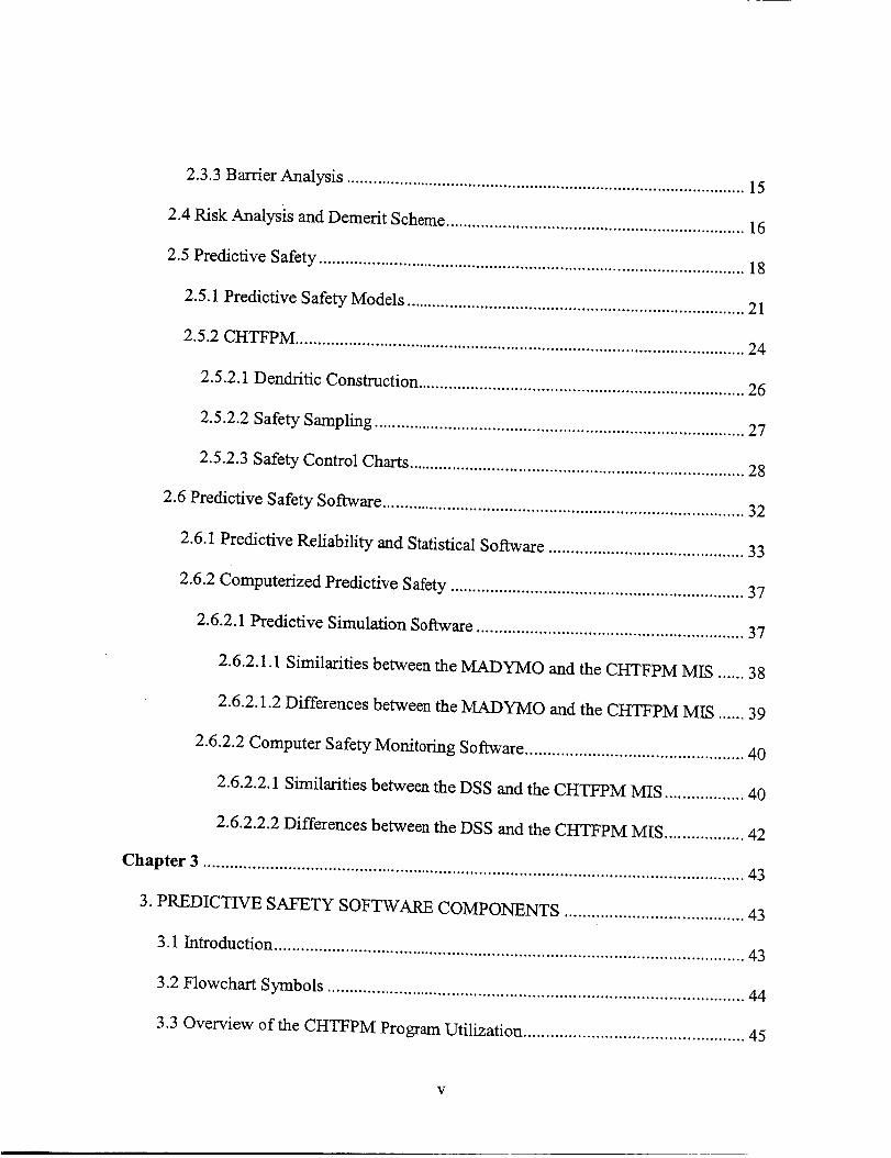
2.3.3 Barrier Analysis ........................................................................................... 15
2.4 Risk Analysis and Demerit Scheme .................................................................... 16
2.5 Predictive Safety ................................................................................................. 18
2.5.1 Predictive Safety Models ............................................................................. 21
2.5.2 CHTFPM ...................................................................................................... 24
2.5.2.1 Dendritic Construction .......................................................................... 26
2.5.2.2 Safety Sampling .................................................................................... 27
2.5.2.3 Safety Control Charts ............................................................................ 28
2.6 Predictive Safety Software .................................................................................. 32
2.6.1 Predictive Reliability and Statistical Sot_vare ............................................ 33
2.6.2 Computerized Predictive Safety .................................................................. 37
2.6.2.1 Predictive Simulation Software ............................................................ 37
2.6.2.1.1 Similarities between the MADYMO and the CHTFPM MIS ...... 38
2.6.2.1.2 Differences between the MADYMO and the CHTFPM MIS ...... 39
2.6.2.2 Computer Safety Monitoring Software ................................................. 40
2.6.2.2.1 Similarities between the DSS and the CHTFPM MIS .................. 40
2.6.2.2.2 Differences between the DSS and the CHTFPM MIS .................. 42
Chapter 3 ......................................................................................................................... 43
3. PREDICTIVE SAFETY SOFTWARE COMPONENTS ........................................ 43
3.1 Introduction ......................................................................................................... 43
3.2 Flowchart Symbols ............................................................................................. 44
3.3 Overview of the CHTFPM Program Utilization ................................................. 45
V
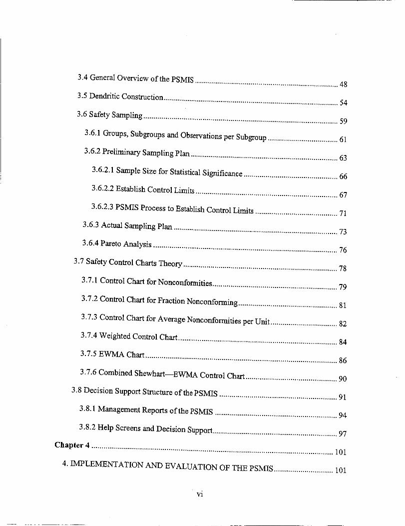
3.4 General Overview of the PSMIS ........................................................................ 48
3.5 Dendritic Construction ........................................................................................ 54
3.6 Safety Sampling .................................................................................................. 59
3.6.1 Groups, Subgroups and Observations per Subgroup ................................... 61
3.6.2 Preliminary Sampling Plan .......................................................................... 63
3.6.2.1 Sample Size for Statistical Significance ............................................... 66
3.6.2.2 Establish Control Limits ....................................................................... 67
3.6.2.3 PSMIS Process to Establish Control Limits ......................................... 71
3.6.3 Actual Sampling Plan .................................................................................. 73
3.6.4 Pareto Analysis ............................................................................................ 76
3.7 Safety Control Charts Theory ............................................................................. 78
3.7.l Control Chart for Nonconformities .............................................................. 79
3.7.2 Control Chart for Fraction Nonconforming ................................................. 81
3.7.3 Control Chart for Average Nonconformities per Unit ................................. 82
3.7.4 Weighted Control Chart ............................................................................... 84
3.7.5 EWMA Chart ............................................................................................... 86
3.7.6 Combined Shewhart--EWMA Control Chart ............................................. 90
3.8 Decision Support Structure of the PSMIS .......................................................... 91
3.8.1 Management Reports of the PSMIS ............................................................ 94
3.8.2 Help Screens and Decision Support ............................................................. 97
Chapter 4 ....................................................................................................................... 101
4. IMPLEMENTATION AND EVALUATION OF THE PSMIS ............................. 101
vi

4.1 Introduction.......................................................................................................101
4.2 Implementation and Evaluation Synopsis of the PSMIS .................................. 102
4.3 Development of Dendritic Elements ................................................................. 103
4.3.1 Preliminary Hazard Analysis ..................................................................... 104
4.3.2 Failure Mode and Effect Analysis ............................................................. 106
4.3.3 Barrier Analysis ......................................................................................... 109
4.3.4 Dendritic Construction ............................................................................... 110
4.4 Design of the Sampling Sheet ........................................................................... 113
4.5 Rational Subgroups, Sample Size and Sampling Plan ...................................... 117
4.6 Statistical Significance ...................................................................................... 119
4.7 Establish Control Limits and Control Charts .................................................... 122
4.7.1 Control Charts for the MSFC Case Study .................................................. 126
4.7.2 Control Charts for the KSC Case Study .................................................... 137
4.8 Reliability and Efficiency of the PSMIS .......................................................... 141
4.8.1 Efficiency of the PSMIS in the MSFC Case Study ................................... 144
4.8.2 Efficiency of the PSMIS in the KSC Case Study ...................................... 146
Chapter S ....................................................................................................................... 149
5. CONCLUSIONS AND RECOMMENDATIONS ................................................. 149
5.1 Introduction ....................................................................................................... 149
5.2 Summary of Work Performed ........................................................................... 149
5.3 Conclusions ....................................................................................................... 151
5.4 Potential Implementation Problems .................................................................. 152
vii

5.5 FutureResearchRecommendations..................................................................154
References......................................................................................................................155
Glossary ......................................................................................................................... 162
APPENDIX A: Preliminary Hazard Analysis for the MSFC Project ............................ 167
APPENDIX B: Failure Mode and Effect Analysis for the MSFC Project .................... 169
APPENDIX C: Barrier Analysis for the MSFC Project ................................................ 173
APPENDIX D: c Control Chart Data for the MSFC Project ......................................... 175
APPENDIX E: Weighted Control Chart Data for the MSFC Project ........................... 177
APPENDIX F: EWMA Control Chart Data for the MSFC Project (2 = 0.4, L = 3.054) 180
APPENDIX G: EWMA Control Chart Data for the MSFC Project ()t = 0.1, L = 2.814) 183
APPENDIX l-I: Preliminary Hazard Analysis for the KSC Project .............................. 186
APPENDIX I: Failure Mode and Effect Analysis for the KSC Project ....................... 190
APPENDIX J: Barrier Analysis for the KSC Project ................................................... 196
APPENDIX K: Classification of Dendritics for the KSC Project .... :............................ 198
APPENDIX L: c Control Chart Data for the KSC Project ........................................... 201
APPENDIX M: Weighted Control Chart Data for the KSC Project .............................. 203
..°
Vlll
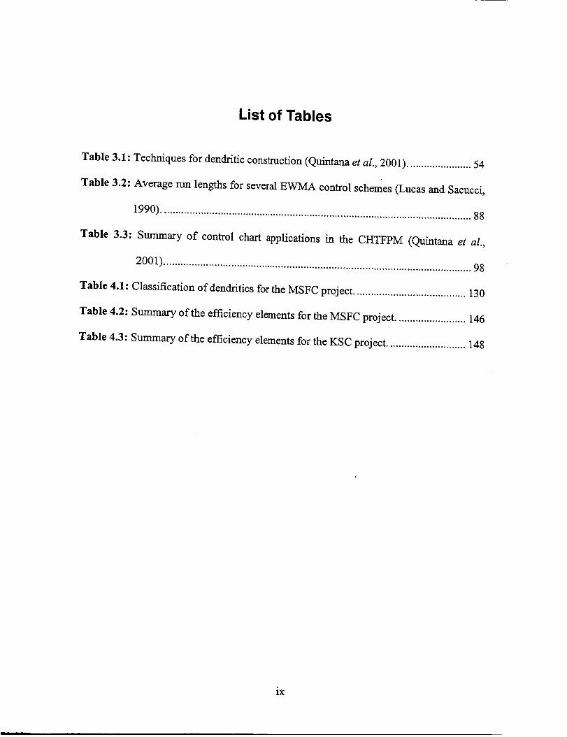
List of Tables
Table 3.1: Techniques for dendritic construction (Quintana et al., 2001) ....................... 54
Table 3.2: Average run lengths for several EWMA control schemes (Lucas and Sacucci,
1990) ............................................................................................................... 88
Table 3.3: Summary of control chart applications in the CHTFPM (Quintana et al.,
2001) .............................................................................................................. 98
Table 4.1: Classification of dendritics for the MSFC project ........................................ 130
Table 4.2: Summary of the efficiency elements for the MSFC project ......................... 146
Table 4.3: Summary of the efficiency elements for the KSC project ............................ 148
ix

List of Figures
Figure 1.1:
Figure 1.2:
Figure 2.1:
Figure 3.1:
Figure 3.2:
Figure 3.3:
Figure 3.4:
Figure 3.5:
Figure 3.6:
Figure 3.7:
Figure 3.8:
Figure
Figure
Figure
Figure
Figure 3.13:
Figure 3.14:
Figure 3.15:
Cross section of the promoted combustion testing chamber ......................... 7
1oint airlock and I-IPGTs located in the cargo bay of the shuttle at KSC ...... 8
Schematic of the CHTFPM (Quintana et al., 2001) .................................... 25
Flowchart symbols and their meanings (Whitten et al., 1989) .................... 44
Flowchart of the entire CHTFPM MIS general process .............................. 47
Schematic of the core events of the PSMIS ................................................. 49
Main menu of the PSMIS ............................................................................ 49
"Delete a project" event of the PSMIS ........................................................ 50
Delete window of the PSMIS ...................................................................... 50
"Exit program" event of the PSMIS ............................................................ 51
Beginning portion of the "Create a new project" event of the PSMIS ........ 52
3.9: New project information screen ................................................................... 53
3.10: Message box indicating that a required field is empty ............................... 53
3.11: Dendritic construction process in the PSMIS ............................................. 56
3.12: Edit feature for the dendritic list ................................................................. 57
Flowchart for assigning weights to dendritics ............................................ 59
Flowchart of preliminary sampling plan .................................................... 65
Flowchart to calculate number of samples needed for statistical
significance ................................................................................................. 68
Figure 3.16: Process that the PSMIS follows when the user estimates /3 ..................... 70
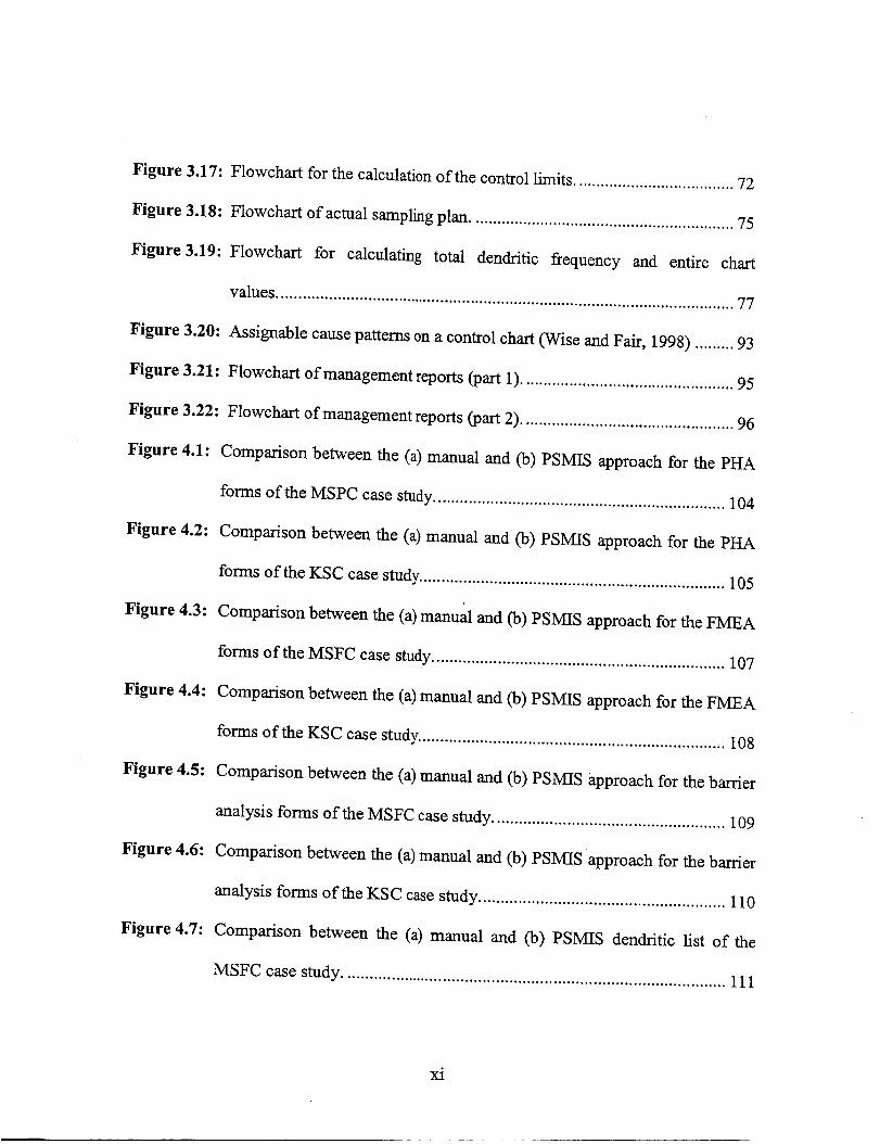
Figure 3.17: Flowchart for the calculation of the control limits ..................................... 72
Figure 3.18: Flowchart of actual sampling plan ............................................................. 75
Figure3.19: Flowchart for calculating total dendritic _equency and entire chart
values .......................................................................................................... 77
Figure 3.20: Assignable cause patterns on a control chart (Wise and Fair, 1998) ......... 93
Figure 3.21: Flowchart of management reports (part 1) ................................................. 95
Figure 3.22: Flowchart of management reports (part 2) ....................... . ......................... 96
Figure 4.1: Comparison between the (a) manual and (b) PSMIS approach for the PHA
forms of the MSPC case study ................................................................... 104
Figure 4.2: Comparison between the (a) manual and (b) PSMIS approach for the PHA
forms of the KSC case study ...................................................................... 105
Figure 4.3: Comparison between the (a) manual and 09) PSMIS approach for the FMEA
forms of the MSFC case study ................................................................... 107
Figure 4.4: Comparison between the (a) manual and (b) PSMIS approach for the FMEA
forms of the KSC case study ...................................................................... 108
Figure 4.5: Comparison between the (a) manual and (b) PSMIS approach for the barrier
analysis forms of the MSFC case study ..................................................... 109
Figure 4.6: Comparison between the (a) manual and (b) PSMIS approach for the barrier
analysis forms of the KSC case study ........................................................ 110
Figure 4.7: Comparison between the (a) manual and (b) PSMIS dendritic list of the
MSFC case study ....................................................................................... 111
xi
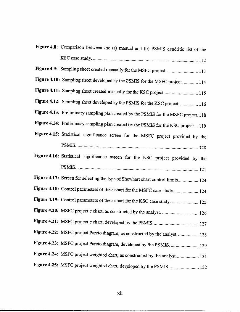
Figure 4.8:
Figure 4.9:
Figure 4.10:
Figure 4.11:
Figure
Figure
Figure
Figure
Comparison between the (a) manual and (b) PSMIS dendritic list of the
KSC case study .......................................................................................... 112
Sampling sheet created manually for the MSFC project ........................... 113
Sampling sheet developed by the PSMIS for the MSFC project ............. 114
Sampling sheet created manually for the KSC project ............................. 115
4.12: Sampling sheet developed by the PSMIS for the KSC project ................ 116
4.13: Preliminary sampling plan created by the PSMIS for the MSFC project. 118
4.14: Preliminary sampling plan created by the PSMIS for the KSC project... 119
4.15: Statistical significance screen for the MSFC project provided by the
PSMIS ...................................................................................................... 120
Figure 4.16: Statistical
Figure 4.17:
Figure 4.18:
Figure 4.19:
significance screen for the KSC project provided by the
PSMIS ..................................................................................................... 121
Screen for selecting the type of Shewhart chart control limits ................. 124
Control parameters of the c chart for the MSFC case study .................... 124
Control parameters of the c chart for the KSC case study ....................... 125
Figure 4.20: MSFC project c chart, as constructed by the analyst ............................... 126
Figure 4.21: MSFC project c chart, developed by the PSMIS ...................................... 127
Figure 4.22: MSFC project Pareto diagram, as constructed by the analyst .................. 128
Figure 4.23: MSFC project Pareto diagram, developed by the PSMIS ........................ 129
Figure 4.24: MSFC proj ect weighted chart, as constructed by the analyst ................... 131
Figure 4.25: MSFC project weighted chart, developed by the PSMIS ......................... 132
xii

Figure 4.26: MSFC project EWMA chart (L = 3.054 and A = 0.4), as constructed by the
analyst ..................................................................................................... !. 133
Figure 4.27: MSFC project EWMA chart (L = 3.054 and ,_ = 0.4), developed by the
PSMIS ...................................................................................................... 133
Figure 4.28: MSFC project EWMA chart (L = 2.814 and _ = 0.1), as constructed by the
analyst ....................................................................................................... 134
Figure 4.29: MSFC project EWMA chart (L = 2.814 and 2 = 0.1), developed by the
PSMIS ................................ . ..................................................................... 135
Figure 4.30: MSFC project combined Shewhart-EWMA chart (L = 2.814 and 2 = 0.1),
as constructed by the analyst .................................................................... 136
Figure 4.31: MSFC project combined Shewhart-EWMA chart (L = 2.814 and _ = 0.1),
developed by the PSMIS .......................................................................... 136
Figure 4.32: KSC project c chart, as constructed by the analyst .................................. 137
Figure 4.33: KSC project c chart, developed by the PSMIS ........................................ 138
Figure 4.34: KSC project Pareto diagram, as constructed by the analyst ..................... 138
Figure 4.35: KSC project Pareto diagram, developed by the PSMIS ........................... 139
Figure 4.36: KSC project weighted chart, as constructed by the analyst ..................... 140
Figure 4.37: KSC project weighted chart, developed by the PSMIS ............................ 141
°,°
XlU

Chapter I
1. INTRODUCTION
This chapter emphasizes the need to look at the concept of safety engineering
from a new perspective: from a proactive, rather than a reactive, point of view. That is,
remedial action should be taken before the fact, instead of after the fact, resulting in safer
and more reliable systems or environments in the workplace. For this reason, predictive
risk analyses have come into an increasing role in providing the most meaningful and
useful information regarding system assessment and system safety (Cooper, 1998). A
predictive safety model for prevention of accidents and system failures, called
Continuous Hazard Tracking and Failure Prediction Methodology (CHTFPM), served as
the foundation for the development of a predictive safety management information
system (PSMIS). This research incorporates the CHTFPM into a software package with a
system's safety decision support structure.
In Section 1.1, the problem is identified concerning the lack safety in industry. A
description of the problem currently faced is given in Section 1.2. The classification of
the problem is described in Section 1.3, followed by Section 1.4 which provides the
rationale for investigating and solving the problem. Section 1.5 gives a brief overview of
the case study scenario that was analyzed in order to test the PSMIS. In Section 1.6, the
scope and purpose of the research is defined. At the end of this chapter, Section 1.7
delineates the organization of the project report.
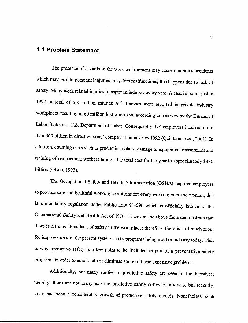
1.1 Problem Statement
2
The presence of hazards in the work environment may cause numerous accidents
which may lead to personnel injuries or system malfunctions; this happens due to lack of
safety. Many work related injuries transpire in industry every year. A case in point, just in
1992, a total of 6.8 million injuries and illnesses were reported in private industry
workplaces resulting in 60 million lost workdays, according to a survey by the Bureau of
Labor Statistics, U.S. Department of Labor. Consequently, US employers incurred more
than $60 billion in direct workers' compensation costs in 1992 (Quintana et aI., 2001). In
addition, counting costs such as production delays, damage to equipment, recruitment and
training of replacement workers brought the total cost for the year to approximately $350
billion (Olsen, 1993).
The Occupational Safety and Health Administration (OSHA) requires employers
to provide safe and healthful working conditions for every working man and woman; this
is a mandatory regulation under Public Law 91-596 which is officially known as the
Occupational Safety and Health Act of 1970. However, the above facts demonstrate that
there is a tremendous lack of safety in the workplace; therefore, there is still much room
for improvement in the present system safety programs being used in industry today. That
is why predictive safety is a key point to be included as part of a preventative safety
programs in order to ameliorate or eliminate some of these expensive problems.
Additionally, not many" studies in predictive safety are seen in the literature;
thereby, there are not many existing predictive safety software products, but recently,
there has been a considerably growth of predictive safety models. Nonetheless, such

models serveto conductsafetyassessmentsfrom a reactive(after-the-fact)point of view
but not from a predictiveor proactiveperspective;this meansthat accidentcausesare
investigatedafter an incidenthastakenplaceto determinewhat mustbe doneto predict
andprevent similar situations.
1.2 Problem Description
Accidents or system malfunctions do not happen unless a hazard exists (Marshall,
1982). Thereby, the tracking of safety hazards is essential to predictive safety, but present
system safety methods typically do not do this (Cooper, 1998). These safety programs are
usually established piecemeal, based on an after-the-fact philosophy of accident
prevention (Roland and Moriarity, 1983). As an illustration, when an accident or system
malfunction occurs, an investigation is conducted to determine the causes. The relevant
causes are then reviewed and discussed to determine what must be done to prevent
similar accidents or malfunctions. Finally, the resulting system modifications or
corrections of design safeguards or procedures are made to existing systems (Quintana et
al., 2001).
What is required is a method or an approach that indicates if the system under
consideration is becoming hazardous; this information would help to check and eliminate
the hazard before accidents can happen. The CHTFPM is an approach that alerts systems
personnel of unsafe situations that could lead to mishaps. The CHTFPM is a new
predictive safety concept which involves a planned, systematically organized, and before-
the-fact process characterized as the identify-analyze-control method of safety. This

predictivesafetymodel usestheprinciplesof work samplingandcontrol charts,thekeys
to trackhazards(Quintanaet al., 2001).
In order to trace hazards, it is imperative to identify the core or unsafe conditions
that can potentially originate them. These core conditions are the building blocks of
hazards and can be termed dendritic elements. Dendrite is a word use by materials
scientists to describe the microstructure of the building blocks of metals (Mangonon,
1999). The development or expansion of multiple dendrites is called dendritic growth,
hence the term dendritic elements or simply dendritics. Thus, the dendritics form the
basis for performing continuous safety sampling to evaluate whether the system is
becoming hazardous, so that proactive actions can be taken to avoid accidents or system
failures.
Besides the lack of predictive safety models that are proactive, these are not
offered or do not exist in a sot_vare application. Therefore, the necessity for developing
satisfactory analysis and predictive methods for software is extremely acute that much
research, effort, and money continues to be spent (Davies et al., 1987). There are,
however, some statistical softwares that employ control charts to determine the stability
of a process or system. Unfortunately, such computer programs do not include the
predictive safety portion, which is the identification of dendritics--the building blocks of
hazards--, and a self-contained, safety focused decision support structure.
1.3 Problem Classification
The problem described in Section 1.2 can be classified as a safety computer

systemchallenge,for an integratedsafetysoftwareapplicationis aproject that is difficult
becauseof theelaborationtime it demands(Wrench,1990).Furthermore,Wrench(1990)
clarifies thatthedevelopmentof a safetymanagementinformationsystem(MIS) requires
sophisticatedtechnology and designof databases,skilled programming, and software
designexperience.As aresult,this kindof problemencompassesanelementarytheme.
The fundamentalsubjectis thatthe developmentof a safetysoftwareapplication
must be a teameffort. In addition,theteamshouldbe comprisedof computersoftware
professionalsand safetyprofessionals(Wrench,1990),which is the pattern followed in
this research.Two graduatestudentsformedtheprojectgroup;oneis a computerscience
major and the other one is a manufacturingengineeringmajor (specializedin safety
engineering).The computerscientistfocusedon the designaspectof the soft-ware--
structure, format, presentation,etc.--while the safety specialist contributed with the
predictive safety part of the software, which is the main topic of this project.
1.4 Rationale for Solving Problem
The goal of this research was to make available the CHTFPM in an easy-to-use
electronic MIS. This means that the theory behind the CHTFPM was integrated in a
single computer program. The intent was that the PSMIS would carry out all
computations automatically in order to facilitate to the user the planning, tracking,
control, management and prediction germane to a system's safety project. Additionally,
the safety status of a system can promptly be known. This signifies that the analyst has a
rapid response to system changes because the user is seeing the effects of the system

6
almost immediately (Mackie, 1998).Moreover,fasterpreventativesafetymeasurescan
be adopted,ensuingin a quickereliminationof thehazard.
It is evident that an integratedMIS approachoffers many advantagesoverhand
computationsandeventraditional computerprograms,like Microsoft Excel, thathelpsin
performingcalculationsand analyzinginformation. The aspect of this approach makes it
easier to exercise control over the calculation processes (Mackie, 1998); furthermore, the
most important benefit is the richer data handling capabilities that are available (Mackie,
2001). Even though the idea of incorporating the CHTFPM into a software packet sounds
attractive, it is not a simple job. Designing a dependable software system that is able to
deliver critical services with a high level of confidence is not an easy task (Ka_aiche et
al., 2002), especially if there are not many predictive safety software applications
available that can act as a benchmark. For this reason there is an urgent necessity of
developing art integrating predictive safety management information system (PSMIS).
1.5 Industrial Scenarios Analyzed
The CHTFPM can be utilized in any industrial scenario in general since it is
robust and, hence, is broadly applicable. To demonstrate the potential utility of the
CHTFPM MIS, it will be tested using two previous predictive safety studies. One of the
investigations was carried out at NASA Marshall Space Flight Center (MSFC) to analyze
the promoted combustion testing chamber operations. The other one was done on the
hoisting operation, testing and preparation of four high-pressure gas tanks (HI:'GTs) at
NASA Kennedy Space Center (KSC).
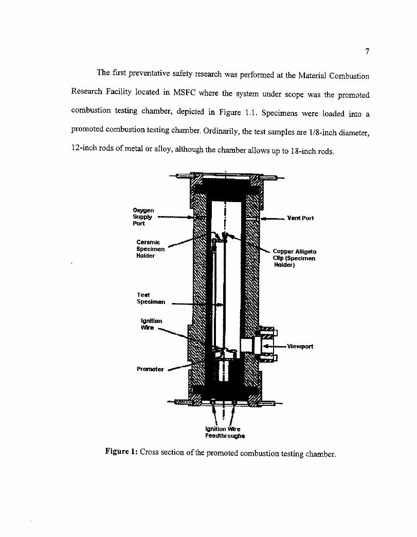
The first preventativesafetyresearchwasperformedat the Material Combustion
ResearchFacility located in MSFC wherethe systemunder scopewas the promoted
combustion testing chamber,depictedin Figure 1.1. Specimenswere loaded into a
promotedcombustiontestingchamber.Ordinarily, thetest samplesare1/8-inchdiameter,
12-inchrodsof metal or alloy, althoughthe chamberallowsup to 18-inchrods.
OxygenSupplyPort
Ceremic
SpecimenHolder
Copper AlligetoClip (SpecimenHolder)
Test
Specimen
IgnitionWire
bort
Promoter
Ignition WireFeedthroughe
Figure 1: Cross section of the promoted combustion testing chamber.

8
After initial placementof thetest sampleinto thepromotedcombustionchamber,
art aluminum igniter is attachedto the sample.The chamber is then filled with 100
percent gaseousoxygen (GOX) bringing the chamberup to the desiredtestpressure,a
maximum of 10,000poundsper squareinch (psi) is allowed. The sampleis ignitedand
allowed to burn. A carbon dioxide laser provides an alternateignition method if so
desired.After the sampleswereignited,the burn length of eachsamplewasrecorded.A
burn lengthof morethan6 inchesonanyonesampleconstitutesfailureof thematerial.
The secondproactivesafetyprojectis basedon four gaseoustanksthat werepart
of a shuttlemission.On July 12, 2001,NASA launchedthe spacevehicle U.S. shuttle
Atlantis: STS-104mission with flight crew 7A aboard.The five-membercrew would
install a new joint airlock aswell astwo oxygenandtwo nitrogengasstoragetankson
the International SpaceStation (ISS).Figure 1.2 showsthe joint airlock and the four
HPGTsbeing loadedin thecargobayof theAtlantis shuttleatKSC.
Figure 1.2: JointairlockandHPGTslocatedin thecargobay of the shuttle at KSC.

The new joint airlock would enablecrews to perform spacewalks without the
presenceof a shuttlewhile recoveringover90 percentof the gasesthat werepreviously
lost whenairlocks wereventedto thevacuumof space.The four high-pressuregastanks
(ttPGTs) would serve to support future station experiments and space walks
(http://www.pao.ksc.nasa.gov/shuttle/summaries/sts 104/index.htm).
The HPGTs, were especially made by a private contractor and tested before being
delivered to NASA KSC. In order to insure 100% reliability of each individual tank, the
staff at KSC decided to again submit the four tanks under more rigorous tests on various
aspects such as pressure and temperature limits, proper functioning of the tanks in
general, etc. During these kinds of tests, the I-IPGTs had to be moved from one place to
another within the same building with a hoist. Thus, the tanks had to be hoisted with
extreme care in order to be displaced to different locations; that is why the hoisting
operation was also a substantial aspect of this particular project.
1.6 Scope and Purpose of Research
The main objective of this research is to develop a computer program that will
facilitate the lengthy and tedious process of predictive a safety management. This
software system will have included the underlying theory of the CHTFPM. A secondary
objective is to make the PSMIS an easy-to-use program, which implies that it must
contain a friendly-user interface, so the analyst can navigate through the program in a
simple manner. Another objective is that the CHTFPM MIS can provide the user with
charts, diagrams and results that are quickly and accurately interpreted.

10
Coupledwith the objectivespreviouslystated,thegoal of this studyis to validate
the performanceof the PSMIS by testing it using the two casescenariosdescribed
previously. The efficiency of the softwareapplicationwill be determinedmainly by the
time andnumberof personsrequiredto completeeachresearchstudywithout the aid of
the CHTFPM MIS relative to whenit was employed.Moreover, the sameinformation
collected pertaining to the studiesexpressedin Section 1.5 will be utilized in the
CHTFPM MIS to observeif the sameresultsareachieved,which havebeenpreviously
validated.
1.7 Organization of the Project Report
This project report is partitioned in five chapters. Chapter 1 has been already
explained, which introduced the current problem that is being faced and the approach that
will be taken to solve such challenge. Chapter 2 gives a detailed review on the literature
pertinent to predictive safety models as well as present soRware programs, along with
their attributes associated with preventative safety. Chapter 3 describes all the
components of both the CHTFPM theory and the PSMIS.
Chapter 4 depicts the implementation and evaluation of the PSMIS by comparing
the results of the PSMIS with the ones obtained in the original studies and by showing the
efficiency of the PSMIS in terms of time and manpower (persons) needed to finish the
projects. Finally, Chapter 5 provides the conclusions and recommendations that will help
for future research.
Chapter 2
2. LITERATURE REVIEW
This chapter consists of the literature pertaining to existing software associated
with safety models and issues, such as predictive safety, hazard tracking and control
charts. Specifically, the most pertinent subjects related to safety analysis will be covered,
especially aspects in the work environment and industry. In addition, the concept of
safety models that predict accidents will be studied; that is, safety methods that serve to
prevent accidents or system failures before they occur.
2.1 Introduction
This chapter begins with a discussion of the concept of system safety in Section
2.2. Section 2.3 covers literature related to hazard analysis with its corresponding salient
topics: PHA, FMEA and Barrier analysis. Section 2.4 describes the concept of risk
analysis and risks classifications. In Section 2.5, the theory of predictive safety is
discussed extensively with some predictive safety models as examples; this section,
additionally, includes a description of the CHTFPM and its components---dendritic
construction, work sampling and control charts. Finally, Section 2.6 provides information
of existing computer predictive safety software.

12
2.2 System Safety
The presence of hazards in the work environment may cause numerous accidents
which may lead to personnel injuries and system failures; this happens due to lack of
safety. For this reason, safety is an essential consideration for all projects (Cheng et al.,
2002). System safety is an element of systems engineering involving the application of
scientific and engineering principles for the timely identification and control of hazards
within the system (Preyssl, 1995).
The safety of the employees and the customers is a principal factor in any process;
that is why the use of system safety programs has grown considerably in the work
environment. Thereby, many industries focus on the safety engineering aspect or their
processes by employing methods and techniques to ensure the safety requirements for the
system are met (Spalding, 1998). For instance, some companies implement in their
facilities safety assessments as part of their system safety programs.
A safety assessment evaluates the safety of the project's output (typically systems
or equipment). Assessments are aimed at providing confn-mation or otherwise of the
project's safety claims. Additionally, they provide evidence for the safety case and should
be viewed as assistance to the project providing necessary confidence as to the integrity
of the system (Spalding, 1998). A pertinent reason of why safety assessments are part of
system safety programs is to assure that any system does not produce an intolerable
degree of risk. There are many different types of safety assessment techniques that assist
in identifying hazardous conditions and risks becoming intolerable; some of the most
commonly known practices are hazard analyses and risk analyses.

13
2.3 Hazard Analysis
According to Lee et al. (1998), new hazards do arise: they must be identified, the
risks assessed and managed. Hazard identification should be used at each stage of any
development or process. In some cases, as the procedure advances in an operation, more
detailed assessment of hazard have to be performed. Once recognized, by an ongoing or
periodic process of review and reporting, the systems personnel must assess the risks
arising from the hazards (Lee et aI., 1998). Wherever achievable, hazards should be
eliminated. Nevertheless, where this is not possible, then the primary means of risk
reduction is to ameliorate the likelihood of the hazard occurring or to minimize the
severity of the accident. There must be a systematic identification and analysis of hazards
related to the system (Spalding, 1998). Thereupon, the following techniques are essential
steps in a hazard analysis:
1. Preliminary Hazard Analysis (PHA).
2. Failure Mode and Effect Analysis (FMEA).
3. Barrier Analysis.
2.3.1 Preliminary Hazard Analysis
A preliminary hazard analysis (PHA) or hazard identification is a systematic,
creative examination of a process or function performed to traverse a representation of
the parts of the system and their interactions (Spalding, 1998), either with other
components or the operators. PHA provides an initial risk assessment of a system,
14
identifies safety critical areas,evaluateshazards,andidentifiesthe safetydesigncriteria
to beused(Grimaldi andSimonds,1989).ThePHA effort shouldthuscommenceduring
the initial phasesof systemdevelopment,or in the caseof a fully operationalsystem,at
the initiation of asafetyevaluation(Quintanaet al., 2001).
In this stage of the investigation, the system is analyzed at the top level to derive a
list of hazards that might be exhibited. Hazard identification is typically carried out using
brainstorming, checklists and/or hazard study techniques. It is also imperative for
credibility that the assessor has the appropriate expertise to assess the project technically.
Thereafter, the evaluator considers the process intention of each component in
turn and by applying a list of guided words attempts to reveal plausible deviations or
anomalies from the process purpose (Spalding, 1998). The hazards associated with the
proposed design or function are identified and evaluated for potential hazard severity,
probability, time of exposure, and hazard classification (Quintana et aI., 2001). As a
consequence, engineering and/or administrative controls as well as other measures
deemed necessary to eradicate or decrease unsafe conditions to a tolerable degree should
be contemplated and recorded.
2.3.2 Failure Mode and Effect Analysis
This phase of the procedure analyzes the system at more detailed levels to derive
the cause-effect chains that could lead to the hazards. The failure mode and effect
analysis (FMEA) is a common technique employed in causal analysis in order to
determine the credible combinations or sequences of causal factors which can lead to
15
hazardous situations. The FMEA requiresa hierarchical breakdownof the system's
structureof functionality (Spalding,1998).
If a possible risk continuesunnoticedby the PHA, the FMEA shouldhelp in
detectingit. FMEA provides furtheranalysisat the lowest level for hazardsidentifiedin
thePHA andcanevenidentify hazardscausedby failuresthat mayhavebeenpreviously
overlookedby the PHA. With FMEA,the analystchoosesa levelof thehierarchyto start
at, considerscomponentsor issuesat a detailedlevel of the hierarchyandrecordstheir
failure modesalongwith causesandeffectsin tabularform (British StandardsInstitution
[BSI], 1991).The failure effectsof thesesubcomponentsthenbecomefailure modesof
components at the next higher level. The procedure may be repeatedto yield the
individual failuremodesof theentiresystem(Spalding,1998).
2.3.3 Barrier. Analysis
At this step of the process, the trace of a threat that could lead to an accident is
analyzed. A barrier analysis is utilized to determine the condition and final consequences
arising from the identified hazards (Spalding, 1998). In addition, a barrier analysis looks
at these potential sources of problems or hazards as well as how the harm or damage
occurred (Wilson et al., 1993). Moreover, it also examines any root cause of the problem
or unwanted event by assessing the adequacy of any installed barriers or safeguards that
should have prevented, or at least mitigated, its occurrence (Quintana et al., 2001).
Barrier analysis defines the basic elements or an undesirable event or problem as
the following (Wilson et al., 1993):
16
1. The threator hazardthat doestheharm
2. The people or thing (target) that is harmed
3. The barrier(s) that could have or should have prevented the threat from reaching
the target
4. The path or trace by which the threat reached the target
There are two kinds of barriers: paper barriers and physical barriers. Paper
barriers may be procedures--norms, standards, rules, etc.--that should be followed when
performing a task. On the other hand, physical barriers may be material objects--special
tools, safeguards, protective equipment, etc.--that serve as an obstacle to prevent the
operator from reaching or going into an unwanted location. It is evident from the
diversity of barriers available for restraining a threat that some barriers will be more
successful than others in providing protection against hazards.
2.4 Risk Analysis and Demerit Scheme
A risk analysis may be performed quantitatively, qualitatively or comparatively
according to the information available. In any case, the purpose of a risk analysis is to
ascertain whether or not the risk has been reduced o a tolerable level or whether further
activities are recommended to minimize it further (Spalding, 1998). The risk levels of
safety systems are described in the legal framework set out by the Health and Safety
Executive (HSE) in 1992 as follows:
1. Intolerable risks. These are risks that are not acceptable under any circumstances.
2. Negligible risks. These are risks that have been reduced to such a low level that no

17
furtherprecautionsaredeemednecessary;the risks is acceptableasis stands.
3. Tolerablerisks. Thesearerisksthatfall betweenthetwo previouscategories,where
therisk is acceptableaslong asit hasbeendecreasedto thelowestlevelpracticable,
bearingin mind thebenefitsflowing from its acceptanceandtakinginto accountthe
costsof furtherreduction.
Put in anotherway, the differenttypesof risks canbe furtherclassifiedinto more
specific categoriesor classesaccordingto the acutenessof the defect.Furthermore,one
of the objectivesof the risk analysisis to quantify uncertaintyand to apply a severity
factor to it (Kaplan, 1991).
To quantifyuncertainty,anumericalscaleis establishedwhich is calledfrequency
distribution. A frequency distribution reflects the variability of a parameterover a
population. In principle, a frequency distribution is measurableby sampling the
population (Montgomery,1996).
Severityrefers to the impactof lossin terms of destroyedproduct,lossin dollars,
damagedequipment/machinery,or degreeof physical impairment (Kaplan, 1991). In
addition, severitymay be time dependent,it may be uncertain,or it may be both time
dependentand uncertain.Using the factors of frequency and severity, a risk analysis
developsclassesof severityandfrequency;theseclassesareusedto rank therelativerisk
of various events.In this research project, a demerit scheme divided in four classes was
employed to classify the dendritics according to their severity. The demerit scheme used
in this study was the same as the one recommended by Montgomery, (1996), which is the
following:

18
1. Class "A" defects - Very serious. This type of defect will render the unit unfit for
service. It will surely cause operating failure of the unit in service that cannot be
readily correct on the job and is liable to cause personal injury or property damage.
2. Class "B" defects - Serious. This defect will probably, but not surely, cause a
Class A operating failure of the unit in service. It will cause trouble of a nature less
than Class A operating failures and will cause increased maintenance or decreased
life.
3. Class "C" defects - Moderately serious. A Class C defect could possibly cause
operating failure of the unit in-service and is likely to cause trouble of a nature less
serious than operating failure as well as increased maintenance or decreased life.
4. Class "D" defects - Not serious. This defect will not cause operating failure of the
unit in service but does account for minor defects of appearance, finish, or
workmanship. This type of defect accounts for major defects of appearance, finish,
or workmanship.
Once all defects or nonconformities are established, they can be grouped in such a
way as to accurately portray the seriousness of a defect when compared to others. By
categorizing the nonconformities (dendritics) into classes, the necessary corrections can
be better directed to the dendritics that require immediate attention, according to their
severity.
2.5 Predictive Safety
Regarding predictive safety studies, there has not been much research directed
19
towardspredictivesafety,but manyparallelsto predictivesafetycanbe drawn from the
subjectof predictivemaintenanceor predictivereliability. The escalatingoperationand
maintenancecostsof modemmanufacturingprocesseshavecauseda searchfor ways to
reducecostswhile maintaininga high level of safetyandreliability (Johnson,1995).A
predictive maintenanceprogramis atool that addressesthis problem--sustainingsafety
and reliability at a low cost--and has becomewidely acceptedthroughout industry
(Shreve,1996). Additionally, the conceptof measuringor foreseeingthe failure of a
machinecomponentis the centralideaof predictivemaintenance.
Underapredictivemaintenanceprogram,conditionsthat causelossof function or
impairedperformanceof a componentor systemare identified andmonitored.Hence,a
corrective actionplan canbe carriedout in the casethat theseconditions areoccurring,
thereby limiting actual in-service failures or failures to operateon demand (Johnson,
1995).In orderto applypredictivemaintenanceto a structure,system,or component,the
failure modes and mechanismassociatedwith theseentities must be identified and
understood.This information is essentialto ensurethat the proper conditions arebeing
monitoredfor effectivemaintenance(ChelbiandAit-Kadi, 1998).
Justas in predictivemaintenance,apredictivesafetyprogrammust also identify
the failure modesandmechanismsassociatedwith systemfailures. The different failure
modes and mechanismsthat need to be identified are the building blocks of hazards;
thesebuilding blocks of hazardsarecalleddendriticelements.Dendriteis a term useby
materialsscientiststo describethemicrostructurebuilding blocks of metals(Mangonon,
1999).The developmentor expansionof multiple dendritesis calleddendritic growth,

20
hengethenamedendritic elementsor simply dendritics.
In an effort to implement an analogy, the materials scienceterm dendrite
(dendritic) is employ in predictive safetyto representthe cornerstoneof hazards.More
exactly, the dendriticsrecognizethe initial causethat givesbirth to a hazard.Thatis why
dendritics are essential factors in forecastingsafety studies becausethey assist in
identifying hazards;subsequently,they canbe eliminatedbefore taking place.Further,
hazardandrisk analysesactaspowerful tools in recognizingthesedendriticsin asystem,
which mayleadto a hazard;more important,thetrackingof safetyhazardsis essentialto
predictive safety (Quintana et al., 2001). The relationship between these two
investigations is that risks arise from hazards; that is, a hazard imports a level of risk.
Once recognized, by an ongoing or periodic process of review and reporting, risks
arising from the hazards can be assessed. Furthermore, corrective action can be taken in
order to prevent any risk before occurring. In other words, these tools alert systems
persormel of unwanted situations; therefore, these safety approaches aid in predicting
system failures or accidents. This means that the risk, thus the probability of an accident,
imported by a hazard can be prevented before occurring, resulting in a predictive and
preventive safety action.
Zissler (1996) notes that after a failure impact is determined, there must be a
means to quantify or measure parameters that will indicate the hazardous condition of the
equipment being monitored. However, choosing which parameters to measure is often the
difficult portion of implementing the predictive safety program (Cheibi and Ait-Kadi,
1998). These parameters are discerned by constantly monitoring the system for the

21
occurrence of specified conditions or dendritics which in return could lead to hazards or
Unacceptable risks. Once the parameters are chosen, the questions of how, when and
where to take such readings must be addressed and determined; all these points provide
the information required to commence the predictive safety plan.
2.5.1 Predictive Safety Models
As was pointed out earlier,amodest amount of researchisfound in the literature
on predictive safety issues. However, these types of studies have been gradually
increasing in the last couple of years since they are a potent, cost-effectivetool.
Predictiverisk(safety)analyses have come intoan increasingrolein providing the most
meaningful and regarding system assessment and system safety (Cooper, 1998). An
advantage of predictivesafetymodels isthatthey arc applicableto many case scenarios
and arethus robust.
For instance,the implementation of thesepredictivesafetyanalysesmay include,
but not limited to: issues in chemical/nuclearplants, environmental issues, traffic
incidents and not to mention industrial/manufacturingprocess. These steadily-rising
models contain similarcharacteristicswhich serve to obtain a common goal, predict
accidents,yet some of thismethods lack in one or more fundamental elements of the
predictionaspect.
For instance,accidentpredictionmodels for urban junctions and road linkswere
developed recentlyand presented in an articlenamed "Accident predictionmodels for
urban roads" (Grcibe, 2002). Such models are explained in '_Uheldsmodel for bygader-

22
Dell: Modeller for 3-og 4-benede kryds. Notat 22, The Danish Road Directorate" (Greibe
and Hemdorff, 1995) and "Uheldsmodel for bygader-Del2: Modeller for straekninger.
Notat 59, The Danish Road Directorate" (Greibe and Hemdorff, 1998).
The main objective of these models is to predict the expected number of
accidents at urban junctions and road links as accurate as possible. In order to develop the
models, detailed information on accident data, traffic flow and road design was collected
fi-om the official accident statistics database covering all police recorded accidents
(Greibe, 2002). These models used information that was previously recorded for
estimating accident prediction.
This kind of data acquisition demonstrates that the data employed in the
calculations were not current, and thus did not provide up-to-the-minute results.
Moreover, these accident prediction programs take a reactive, instead of a proactive,
approach to predict or prevent similar anomailies. In other words, when an accident
arises, an investigation is conducted to determine the causes. The relevant causes are then
reviewed and discussed to determine what needs to be done to prevent similar accidents.
These safety programs are usually established piecemeal, based on an after-the-
fact philosophy of accident prevention (Roland and Moriarity, 1983). The tracking of
safety hazards is essential to predictive safety, and present system safety methods
typically do no do this (Cooper, 1998). In addition, these models did not employ control
charts, the keys for predictive safety (Quintana et al., 2001), to determine if the roads
were operating under the presence of hazards.

23
Another example of a predictive safety method is a safety monitoring model
which evaluated the performance of road programs. This model was described in a
published paper labeled "Monitoring performance of road programmes in New Zealand"
(Guria and Mara, 2000). Such approach was based on developing a control chart system
to identify the occurrence of actual risk changes or deviation from the expected level. In
addition, these control charts were utilized to monitor fatalities. Unlike the previous
models described, this one employed new real time data to perform the analysis. The data
was incorporated in the control charts to identify the risk changes, so that necessary
measures could be undertaken.
Nonetheless, an inconvenience of this model is that charts can be developed on
monthly or weekly basis. Monthly charts have an advantage of a longer period of time
during which the random ups and downs are smoothed; this issue is particularly
important for fatalities. However, a disadvantage is that it takes a long period of time to
get an indication of any risk changes. Weekly charts, on the other hand, have the
disadvantage of short time period. A crash with relatively large number of deaths
indicates occurrence of an unexpected phenomenon while its occurrence is possible due
to randomness. This needs to be taken into consideration while interpreting the charts.
An advantage of the weekly chart, relative to the monthly chart, is that within a
few weeks it provides an indication of any risks changes. However, although this
monitoring safety model utilizes up to date information and control charts to spot any
variations in road safety, it still has the disadvantage of not giving descriptive safety
statistics of a system on a daily basis. This means that a considerably amount of time has

24
to passby in order to obtain anyvaluableinsight on the safetystatusof a system,even
whenweekly chartsareused.
Therefore,a more completeand reliable predictive safetymodel that hasbeen
developed,entitled ContinuousHazardTracking and Failure Prediction Methodology
(CHTFPM), will be employedin thisresearchbecauseit addressesthe lacking traits of
existingpredictive safetymodels.Somemissingattributesof presentanticipatorysafety
modelswhich aremetby the CHTFPMareutilizing real-timeor currentdata,makinguse
of control charts to determine the safety statusof the system,and providing those
diagramsalmost immediately,evenon a daily basis.Moreover,the CHTFPM predicts
accidentsandsystemsfailuresbeforetheyreachtheuseror affectthe system.
2.5.2 CHTFPM
The Continuous Hazard Tracking and Failure Prediction Methodology
(CHTFPM) is a predictive safety model. It involves a process that is well planned,
systematically organized, and before-the-fact and which is characterized as the identify-
analyze-control method of safety (Quintana et al., 2001). This methodology looks at the
concept of safety from a proactive, rather than a reactive, perspective; that is, remedial
action is taken before the fact, instead of after the fact. The way the model achieves the
previous objective is by tracking a system for the occurrence of conditions becoming
unsafe. Then it alerts safety managers or systems personnel of the hazardous conditions
previous to happening; therefore, corrective action can be taken before the risks activate,
hence, resulting in a proactive safety measure.
25
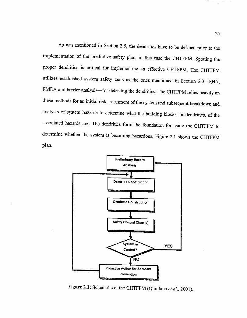
As was mentionedin Section2.5, the dendriticshave to be definedprior to the
implementation of the predictive safetyplan, in this casethe CHTFPM. Spottingthe
proper dendritics is critical for implementingan effective CHTFPM. The CHTFPM
utilizes establishedsystem safety tools as the ones mentionedin Section 2.3--pHA,
FMEA andbarrieranalysis--for detectingthedendritics.The CHTFPMreliesheavilyon
thesemethodsfor an initial risk assessmentof the systemandsubsequentbreakdownand
analysisof systemhazardsto determinewhat the building blocks,or dendritics,of the
associatedhazardsare. The dendriticsform the foundation for using the CHTFPM to
determinewhether the systemis becominghazardous.Figure 2.1 showsthe CHTFPM
plan.
l Preliminary Hazard I_Analysis
[ Oendri'icCon=ruCtionI
Dendritic Construction I
tI I....
_m_ Proactive Action for Accident ]
___....... Prevention I
YES
Figure 2.1: Schematic of the CHTFPM (Quintana et al., 2001).

26
It is importantto emphasizethatthe effectivenessof theCHTFPM dependson the
identification of the dendritics;thesebuilding blocks of hazardsareuse for performing
the sampling study of a given system.In addition to the identification of dendritic
elements,the CHTFPM utilizes conceptsunderlying the predictiveapproachto system
which arederived from work samplingand control chart theories,the keysto tracking
hazards(Quintanaet al., 2001).
2.5.2.1 Dendritic Construction
As was explained in Section 2.5, the dendritics have to be defined first in order to
implement the CHTFPM. Recognizing the proper dendritics is critical for implementing
an effective CHTFPM. Many of these dendritics or defects emerge due to human error.
According to Marcombe (1993), accidents-injuries and the disruption of scheduled
system operation caused by human element factors shows that the human element is a
very significant factor affecting the safety of systems. Unfortunately, many system
predictive methods are based solely on equipment failures neglecting the human
interaction of man-machine systems (Koval, 1997). Therefore, it is enormously vital for
credibility that the analyst has the appropriate expertise to assess the project not only
technically but also taking into consideration the human interaction with the system.
The CHTFPM employs the previously described PHA, FMEA and barrier
analysis, for detecting the dendritics; that is, the CHTFPM strongly relies on these
techniques for dendritic construction. The reason why the CHTFPM uses these
approaches is because they can be applied to human factors analysis. Defining unsafe
27
behavior of operators is important when consideringoverall system safety. When
constructing the dendritics for a given system,the humaninteractionwith the system
cannotbe ignoredandmustbe included(Camet,1999).
The way the CHTFPM elaboratesa list of dendritics is by analyzingand
reviewing with detail eachentry of thePHA, FMEA andbarrier analysis.Afterwards,a
preliminary dendritic list is formed by choosingthe items that will lead to possible
occurrenceswhich could result in systemfailure or employeeinjury--sometimes the
humanis consideredasthe system.Finally, the initial dendriticrecordis double-checked
for any repeatingor similar elementsandto enhancethewording of the items,ensuingin
the concludingversionof thedendriticlist. Nevertheless,thefinal list of dendriticscanbe
modified if more defectsor hazardousconditions are found since undetectedor new
hazardsmay arise. As indicated by Lee et al. (1998), sometimes as the procedure
advances in an operation, more detailed assessment of hazards has to be performed.
2.5.2.2 Safety Sampling
Safety sampling or work sampling is originated from probability conditions. A
work sampling investigation consists of a number of random observations taken at
different intervals in time. CHTFPM utilizes the principles of monitoring, trending and
pattern recognition to draw inferences. The CHTFPM model emphasizes the application
of work sampling theory in order to prevent undue risks and accidents. According to
Meister (1985), accidents are preventable. This prevention is hardly attained and is
achieved by employing an immense amount of effort conducting periodic, thorough

28
inspectionsandvigilance onthepartof operationssupervisors.Nonetheless,avoidanceof
unwanted,grave situationscan be lessdifficult if work sampling and control charts,
taking advantageof thedendriticslist, supplementsafetyinspections.
The CHTFPM conductswork samplingin arandomfashion,ratherthanat fixed
periods of time, which is the way safety inspectionsareperformed.Moreover, work
samplingis usedin the CHTFPM asaplain way to presentameasureof the tendencyof
the systemin a productiveand cost-effectivemanner.Justaswork samplingis usedto
give a measurementof over-allperformance,thesamplingin CHTFPM givesanover-all
view of the safetystatusof the systemunder observation(Career,1999).If the system
exhibits symptomsof becomingharmful,then effectivecontrol measurescanbe carried
to preservea desireddegreeof safety;hence,resulting in preventionof anundesirable,
severeconsequence.
2.5.2.3 Safety Control Charts
The core of the CHTFPM is to monitor the system to identify the dendritics that
lead to hazards. The control charts incorporate these dendritics into graphs to indicate if
the system is out of control when the system is operating under the presence of these
defects. In the predictive safety model CHTFPM, control charts are used to measure the
tendency of a system when is becoming hazardous. After sampling is performed, a
control chart is constructed graphically by means of a characteristic that has been
measured or computed, with a predetermined level of safety.
29
The chart containsa centerline that representsthe averagevalue of the quality
characteristic correspondingto the in-control state (Montgomery, 1996). Two outer
horizontal lines called the uppercontrollimit (UCL) andthe lower control limit (LCL)
arealso shownon the charts. Thesecontrol limits arechosenso that if the systemis in
control, nearly all of thesamplepointswill fall betweenthem. If no points go outside the
bands, it is not necessary to take corrective action. On the contrary, if a point is outside
the bands or limits, it means that a hazard is present or that the system is out of control,
requires immediate attention. Thus, the control charts are powerful instruments for
stabilizing and controlling the system or process at desired operability levels. The
advantages of control chart applications in industry are listed as follows (Montgomery,
1996):
1. Control charts are a proven technique for improving productivity. Just as control
charts improve productivity, they are used to improve the safety status of a given
system in the CHTFPM. The control chart provides the technique to evaluate
system safety as well as measure the success of corrective actions.
2. Control charts are effective in defect prevention. The control charts utilized by the
CHTFPM are effective in hazard prevention. By detecting the conditions that lead
to hazards, dendritics, the control chart provides the impetus to act and correct the
conditions before hazardous conditions or unacceptable risks occur.
3. Control charts prevent unnecessary process adjustment. The control charts in the
CHTFPM indicate when corrective actions need to be taken, by indicating out-of-
control situations, thus preventing unnecessary system adjustments.
30
4. Control chartsprovidediagnosticinformation. Analysis of the control charts in the
CHTFPM can yield information on the safety status of the system under
observation. By indicating when the system went out-of-control, the control chart
actually directs the efforts of the system analyst in investigating the causes of
accidents or system malfunctions.
5. Control charts provide information about process capability. The control charts in
the CHTFPM provide an overall view of system safety and give a good indication
of the relative degree of safety that the system possesses.
The control charts described previously are usually called Shewhart control
charts, as they are based on the principles of control charts developed by Dr. Walter A.
Shewhart (Montgomery, 1996). The signal that the process may be out of control,
ignoring the use of runs testing, is the occurrence of a single point outside the 3or limits
(Hunter, 1986). Even though Shewhart control charts have many advantages, they are
relative insensitive to small shifts in the process, on the order of about 1.5cr or less (Ryan,
1989).
That is why one alternative to the Shewhart control chart may be used when small
shifts in the process are of interest: the exponentially weighted moving average (EWMA)
control chart (Hunter, 1986). The performance of the EWMA control chart is, in some
ways, easier to set up and operate. The EWMA control chart can be viewed as a method
for establishing real-time dynamic control of the process being monitored (Hunter, 1986).
The EW-MA control chart can be used in CHTFPM when the risks of not detecting small
shifts in the safety mean of the system under observation rise to unacceptable levels.

31
As mentionedearlier, the EWMA performswell detectingsmall shiftsbut does
not reactto large shifts asquickly asthe Shewhartcontrol chart.A goodway to further
improve the sensitivity of the control procedureto large shifts without sacrificing the
ability to detect small shifts quickly is to combine a Shewhartcontrol chart with the
EWMA (Borror et al., 1998).These combined Shewhart-EWMA control procedures are
effective against both large and small shifts. It is also possible to plot both the Shewhart
chart and the EWMA chart on the same chart along with the associated control limits for
each chart (Hunter, 1986). The use of either the Shewhart control charts or the EWMA
control chart, or both, in CHTFPM depends upon the nature of the system being analyzed
and the desired protection fi:om risks and unacceptable hazards. The EWMA control chart
as well as the different kinds of Shewhart control charts and the associated equations for
their construction will be discussed in further detail in Chapter 3.
Besides the utilization of control charts, the Pareto analysis is a useful tool in
knowing which dendritics required immediate attention. The relationship between these
two techniques is that the control chart indicates if there is reason to suspect that the
system may be becoming hazardous with respect to the sampled dendritics; consequently,
this result provides the rationale to carry out a more comprehensive study of individual
dendritic occurrences using Pareto analysis. This will provide an indication about which
one of the dendritics has the highest frequency of occurrence; thus necessary and
proactive measures can be taken more specifically for accident prevention.

32
2.6 Predictive Safety Software
With the rapid evolution of technology, there is a swift increase and development
of computer software. This proliferation of software has emerged in almost any area and
field of study there is: medicine, science, engineering, etc. The aim and scope of this
section consists of the literature concerning existing software associated with predictive
safety. To be more precise, only the most relevant topics related to preventative safety
analysis will be covered. In addition, the concept of safety models that intent to predict
accidents will be studied; that is, safety methods that serve to prevent accidents or system
failures, especially in an electronic or automatic manner, before they occur.
The purpose of this project is to integrate the CHTFPM in a computer software
package. That is, the intent of this study is to use the underlying theory of the CHTFPM
described in all the previous sections of this chapter in a single, simple electronic
management information system (MIS). The intended predictive safety software will
carry out all computations and will provide the user (analyst or assessor) the adequate
graphs such as Pareto diagrams or control charts, as requested. By this means, the safety
status of the system under consideration will be quickly available; with this attribute, a
greater degree of interaction with the software can be achieved. This is especially true in
the area of rapid response to system changes because the user is seeing the effects of the
system almost immediately, and thereby, a greater level of interaction being released
(Mackie, 1998). Furthermore, faster preventative safety measures can be adopted, giving
as a result an earlier cancellation of the hazard.
33
2.6.1 Predictive Reliability and Statistical Software
Not many studies in predictive safety are seen in the literature; thereby, there are
not many existing predictive safety sott'ware products. Most of the available safety
computer systems serve to conduct safety assessments from a reactive (after-the-fact)
point of view but not from a predictive or proactive perspective. Lately, there has been a
considerably growth of predictive safety models; nonetheless, such models--as the ones
revealed in Section 2.5.1--are not offered in a software package. Therefore, the necessity
for developing satisfactory analysis and predictive methods for software is so acute that
much research, effort, and money, continues to be spent (Davies et al., 1987).
In addition, evoking from Section 2.5, predictive safety can be drawn in parallel
from the subject of predictive maintenance or predictive reliability. In this topic, there are¢
several software applications, such as Alvey and Esprit programmes; additionally,
Proportional Hazard Modeling methods for software reliability data were largely
developed (Davies et al., 1987). For predictive reliability software, in particular, analyst
have focused upon these methods as a systematic approach to the incorporation of the
wealth of supplementary information often available in software development or soft-ware
reliability databases (Davies et al., 1987). Some early work in this area was undertaken
by Boeing in the USA (Nagel and Skrivan, 1981) and continuing interest was followed in
France (Font, 1985); moreover, Wightman and Bendell (1986) were the ones to apply
Proportional Hazards modeling to reliability software.
At the beginning of the 1980's, a typical software reliability prediction method
required data comprising a history of the times at which individual failures occurred
34
(Dale andFoster, 1987),This typical quality, similar to thepredictivemodelselucidated
in Section 2.5.1, manifeststhat suchreliability predictivemethodsneededinformation
that was previously recorded for estimating failure prediction. This mode of data
acquisition demonstratesthat the data employedin the calculationswas not current,
which is preferablesothat moremodemresultscanbe obtained,leadingto moreaccurate
deductions.Likewise, these reliability prediction programs also adopteda reactive,
insteadof a proactive, approachto foreseesimilar systembreakdowns.As per Roland
and Moriarty (1983), these safety (reliability) programs are usually established
piecemeal,basedon anafter-the-factphilosophyof accidentprevention.In order to be
proactive, the tracking of safety hazardsis essentialto predictive safety, and present
systemsafetymethodstypically donodo this (Cooper,1998),includingpredictivesafety
computerapplications.
Another major featurein the 70's and early 80's of reliability softwarewas the
incorporation of statisticalmodels proposedfor assessmentand prediction (Veeverset
al., 1987). However, some approaches back then carried a heavy computational burden,
and hence statistical methods were not readily implementable for software applications;
even more, this state of affairs reflected the fact that no software reliability model was
generally useful or applicable (Veevers et al., 1987). The difficult interpretation by the
non-statistician and the inappropriateness of the predictive statistical methods for
software applications were mainly due to the fact that in the past this type of software did
not have a user-friendly interface such as a Windows cnviromnent. The CHTFPM
software addresses and meets these issues---data presented in an easy-to-understand
35
mannerand generallyapplicableto different casestudies.In presenttimes,incorporation
of statisticalmethodsin sottwarereliability prediction is feasible(Veeverset aI., 1987);
in fact, various statistical software packages, like MINITAB, DATAPAC, etc., are
available for statistical analysis of data including virtually all types of control charts.
Today's statistical software can calculate the sample parameters, initial control
limits and control charts. Most sottware can provide additional summaries and analyses
such as listings of the raw data, out-of-specifications values, histograms, checks for runs
and other patterns within control limits, tests for normality, process capability
calculations, Pareto analyses, and trend analyses (Juran, 1988). Unfortunately, such
software programs are only for statistical purposes and do not take into account the safety
aspects of a project, especially the human interaction portion. In the words of Koval
(1997), many reliability or statistical predictive methods are based solely on equipment
failures neglecting the human interaction of man-machine systems. This signifies that the
statistical programs do not typically provide dendritic identification capabilities.
Furthermore, the safety information would have to be stored by the analyst in a
different location from the statistical program, either on paper or electronically.
Therefore, in a predictive safety study, safety data would have to be first stored in one
location (database, paper files, etc.) and then extracted from its original site and input
again in the statistical software for calculations. This reflects that the inputting of data has
to be done twice which, apart from interaction inefficiencies, could lead to possible
mistakes (misinterpretation or human error) at the time of re-entering the data, resulting
in erroneous conclusions.

36
TheCHTFPM softwarewill comprisethe safetyandstatisticalaspectstogetherin
one, singlesoftwareapplication;this implies that the safetyinformationwill be savedin
the sameprogram where the statistical computationswill be executed.To be more
precise, safety records and/or reports will be kept in a databasecontainedin the
CHTFPM computerprogram.Gettinginformationout of therecords,however,is acause
of frequent frustration, which is why professionalsneed to look critically at their
recordkeepingpracticesfrom gatheringdatato providing information (Wrench,1990).It
is strongly recommended,therefore,to use databasesto store safety recordsand/or
information.
That is why Wrench (1990) urges each health and safety professional to calculate
on an annual basis the cost in time to produce every record in the office, the cost of the
space the records occupy, the cost of the cabinets and shelves they fill, and the cost of the
time spent in trying to find data when needed. An examination of this sort can be
revealing since the cost is likely to equal or surpass the cost of the personnel hired to
ensure company health and safety. If this lesson were taken to heart, controls would be
instituted and an immediate effort would be made to computerize. Moreover, by having
safety reports together with the statistical portion in the same so,are package, records
will not have to be re-entered, thus, no faults due to human error will be exhibited. In
fact, the reckonings will be carried out automatically after the safety data has been
recorded.
Besides keeping safety records outside the statistical computer system, current
statistical software products do not offer the user suggestions or recommendations for

37
performing calculations.For instance,the analystmay try to use ap chart to analyze
some data; however, such information is best represented by a c chart. Consequently, the
results may not be accurate, leading to false conclusions or wrong interpretations. The
CHTFPM will also tackle this limitation; it will supply to the assessor the suggestions
and options of what type of analyses are more adequately suited for the data collected,
according to the circumstances of the system under observation.
2.6.2 Computerized Predictive Safety
In conjunction with predictive reliability and statistical soil-ware, there exist
simulation methods and computer aided safety monitoring whose loci are linked to
predictive safety. These computer approaches monitor systems and analyze collected data
to identify possible causes of adverse or hazardous conditions. Thus, prediction of
anomalies and concomitant appropriate actions can be taken to prevent system failures
and accidents. Some existing computerized safety monitoring and prediction systems are
like the CHTFPM software application in various aspects. The similarities and
differences between these computerized methodologies and the CHTFPM computer
program are discussed in this section.
2.6.2.1 Predictive Simulation Software
In a traffic accident prediction study, injury potential of a safety design feature is
predicted by using laboratory/mathematical simulation data of traffic accidents (Norin
38
and Isaksson-Hellman,1995).The researchstatesthat mathematicalsimulationscould
predict by correlationthe type of injuriesin a certainaccidentconfigurationbeforethe
systemis exposedto harmful circumstances(in this investigationthe humanwas the
system). In this report, MADYMO mathematicalsimulation sottwaremodels (TNO,
1990) areused.The MADYMO simulationmodelswere validated for Volvo 240 cars
from full scalecrashesat severalspeedsand from a Hyge sledtest series(Norin et al.,
1991). This computer/mathematical simulation method has several similarities to the
CHTFPM soil-ware program.
2.6.2.1.1 Similarities between the MADYMO and the CHTFPM MIS
The first similarity of MADYMO with the CHTFPM MIS is that such approach is
proactive, which means that it can predict accident likelihood (in this case risk injuries) in
advance, hence, influence the design and manufacturing of the vehicle before a mishap
reaches the user. As indicated by the article, the purpose of this method is to create a
means of predicting to what extent a component of a car can influence the risk of injury
before the system is exposed to real traffic conditions. By paying particular attention to
such components, corrective action can take place before the driver is exposed to hazards
(Norin and Isaksson-Hellman, 1995).
A second similarity this computer simulation model has with the CHTFPM
electronic version is that it can be generalized or applicable for other protection systems
and for other accident types (Norin and Isaksson-Hellman, 1995). A third likeness is that
the mathematical safety simulation approach, just as the computerized CHTFPM, utilizes

39
a largeamountof current information collected in new real- time from the experiments to
perform calculations. This indicates that data from preceding or previous accidents was
not employed--instead, in-progress data was used--to predict accidents.
A fourth similarity between the two compared models is that both take into
account the human interaction with the machines. In the case of the MADYMO
simulation methodology, the machine is the car, and the human interaction parameters
considered are occupant size, seating position, among others. (Norin and Isaksson-
Hellman, 1995). A functioning of a system must consider the human-system where the
humans are involved with it (Bologna and Hollnagel, 2002). The person's behavior has to
be defined and quantified when considering overall system safety.
2.6.2.1.2 Differences between the MADYMO and the CHTFPM MIS
Just as this method has similarities to the CHTFPM MIS, it also has
dissimilarities. Unlike the CHTFPM computer system which displays control charts, the
MADYMO application only provides distribution graphs to make inferences about the
safety standing of the system.
Another difference there is between the two is that the mathematical MADYMO
model always implies a simplified description of reality and certain faults (errors) occur
with such generalization (Norin and Isaksson-Hellman, 1995). This denotes that such
software does not quantify possible error of the results, whereas the CHTFPM program
does.
40
2.6.2.2 Computer Safety Monitoring Software
An additional safety software application is a safety monitoring computer
program that measures adverse conditions in the system requiring attention; thus, such
unacceptable situations can be addressed and solved before resulting in an accident. A
construction report written by Cheng et al. (2002) focuses on describing the development
of a decision support system (DSS) for safety monitoring of excavations in construction
sites. This computer system is designed to assist construction engineers in monitoring and
controlling the excavation conditions that could become hazardous with the aid of
instruments (wall inclinometer, strut and rebax strain gages, etc.) placed in the
construction field. Like the previously depicted computer simulation system
(MADYMO), the DSS also has various analogous aspects to the CHTFPM MIS.
2.6.2.2.1 Similarities between the DSS and the CHTFPM MIS
One identical feature to the CHTFPM MIS is that the DSS is a before-the-fact
safety technique, which implies that its predictive aspect prevents accidents due to the
fact that corrective action can take place before they can occur. As sustained in the
articles, predictions of adverse conditions and appropriate actions can be taken to prevent
construction accidents (Cheng et al., 2002). Another equal attribute the DSS has with
respect to the CHTFPM computer software is that it utilizes present-day information,
gathered from the instruments located in the construction field, to perform computations
which entail the safety state of the system.

41
An additionalcharacteristicof theDSSis thatit helpsidentify possiblecausesand
origins of hazardousconditions(Chenget al., 2002). This is an analogy of the FMEA and
dendritic qualities, respectively, of the CHTFPM software application. More exactly, the
possible causes of adverse conditions in the DSS resemble the causes of the failure modes
depicted in an FMEA (which is enclosed in the CHTFPM computer program). In the
same way, the possible origins of unacceptable situations in the DSS are analogous to the
dendritics (building blocks of hazards) in the CHTFPM software package.
One more comparable element between the DSS and the CHTFPM sottware
program is that both employ databases to store safety information in the same application
where the reckonings are realized. The use of databases is highly recommended since it
facilitates data handling/management. In effect, by applying open database connectivity,
the program data interface writes/reads the information to/from the associated databases,
respectively. Moreover, through this process, the stored safety data files can act as the
communication media (Cheng et al., 2002).
A final, similar mark to the CHTFPM MIS is that the DSS is a PC-based software
program. The prime development tools of the DSS include Visual Basic, MS Excel,
Access and MapInfo, which were developed in a Windows environment. Further, the user
communicates with the system components through a custom interface developed with
Visual Basic (Cheng et al., 2002). All the previously defined points are also part of the
CHTFPM sottware, including the use of Access as a platform. Additionally, just like the
computerized CHTFPM, the DSS when compared with manual methods--significantly

42
improves automation in safety monitoring, enhancescomputationalefficiency and
increasesdataaccuracyandconsistency(Chenget al., 2002).
2.6.2.2.2 Differences between the DSS and the CHTFPM MIS
In the same manner the MADYMO computer simulation system has some
distinctions from the CHTFPM software, the DSS computer program differs from the
CHTFPM MIS as well. For example, an obvious dissimilarity is that the DSS does not
use control charts as the source for portraying the system's safety status. The DSS, rather,
displays graphical trends as well as data distribution plots that depict the safety degree of
the scheme and estimates possible accident likelihood.
In addition to not utilizing control charts, the DSS differs fzom the CHTFPM
software packet because the first method is not generally applicable, while the CHTFPM
MIS is robust. Although the DSS is applicable within the subject of construction work, it
is inappropriate for other case scenarios since it requires special equipment or
instrumentation absolutely used in construction.
The last difference between the DSS and the computerized CHTFPM is that the
DSS is costly to use. The electronic CHTFPM, however, is a cost-effective tool because
it does not require any additional allocation of resources (Quintana et al., 2001). The
DSS, on the other hand, collects and transmits measured data from the construction
ground to the job site office using automated transmission technology through cable
connections or wireless communication. Therefore, this factor, besides the measuring
instruments, contributes to a high cost to implement such a safety monitoring system.

Chapter 3
3. PREDICTIVE SAFETY SOFTWARE COMPONENTS
The focal point of this study is to incorporate the theory behind the CHTFPM into
a software package; therefore, this chapter describes the CHTFPM constituents both in
theory and in the computer program. First, an overview of the ingredients of this
predictive safety model will be explained in order to understand how the predictive safety
management information system (PSMIS) will work. Subsequently, the integration of the
CHTFPM elements into a programmable system will be depicted in the form of
flowcharts to portray the functioning of the CHTFPM MIS.
3.1 Introduction
This chapter exposes in Section 3.2 the flowchart symbols used in the program
design of the PSMIS as well as their meaning. In Section 3.3, an overview of the entire
program utilization is provided, followed by general overview of the sot'tware package in
Section 3.4. The construction of dendritics is explained in Section 3.5. Section 3.6 talks
about the preliminary samples needed to establish control limits. Control chart theory is
presented in Section 3.7. Section 3.8, describes the topics related to safety sampling. In
Section 3.9, the Pareto analysis is elucidated. Finally, Section 3.10 consists of the help
and decision support offered to the user.

44
3.2 Flowchart Symbols
Before revealing the CHTFPM components in theory as well as in a flowchart
fashion, it is essential to understand the meaning of symbols employed in the diagrams
that show how the MIS will carry out a certain process or task. A reason for choosing
flowcharts to explain the process of the predictive safety computer system is because
program design frequently involves the use of flowcharts (Whitten et al., 1989). In
addition, system flowcharts were one of the very first tools commonly used by systems
analysts and computer programmers.
The American National Standards Institute (ANSI) has established certain
symbols that have been widely used n the computer industry to describe the logic of both
systems and computer programs (Whitten et aI., 1989). The symbols that were utilized in
the flowcharts for the development of the PSMIS are depicted in Figure 3.1 together with
their meaning according to the ANSI standards:
Process
- Input Start / End)
operation Output
Internal
storage
Print / tDocument
__J
i IO'-°.oe
Sequence ofactivities
Figure 3.1: Flowchart symbols and their meanings (Whitten et al., 1989).

45
Another causefor using flowchartsin the developmentof PSMIS is because,
given the appropriatediagrammingtechniques,it is much easier to describecomplex
activities andproceduresin diagramsthan in text (Martin, 1987).A picturecanbemuch
better than a thousandwords becauseit is concise,precise and clear. Furthermore,
systemsflowcharts arethebasisfor communicationbetweenend-user,systemsanalysts,
computeroperationspersonnelandcomputerprogrammers(Whitten et aI., 1989).
3.3 Overview of the CHTFPM Program Utilization
This section presents an outline and a general idea of the underlying theory of the
CHTFPM, which consists of identifying the dendritics of a system--the building blocks
of hazards. Founded on this rationale, the first step of the PSMIS, or CHTFPM MIS, is to
construct the list of dendritics based on the reports of the PHA, FMEA and barrier
analysis. Second, sampling has to be carried out to determine the number of samples
needed for statistical significance and to establish the control limits. From these
preliminary samples, a Pareto diagram can be constructed according to the cumulative
frequencies of the observed dendritics.
In order to conduct the initial observations, the computer program provides the
user with sampling sheets in the form of reports to document the occurrence of dendritics.
After deciding to set up the control limits, the type of control chart must be selected so
that the respective control chart parameters can be calculated. Once the type of control
chart has been chosen to represent the safety status of a system, the control limits can be
computed and implemented to measure the safety level of the process. Before plotting

46
points on the control chart, a safetysamplingschememustbe createdin orderto begin
collecting data.Suchdatawill bemappedon thecontrol chartalterthe samplingplanhas
beendeveloped.
From the acquiredinformation using the designedsampling scheme,a Pareto
diagramcanbe obtainedto depict thedendriticsthat occurmoreoften.Whenplotting the
points on the control chart, it canbeseenif thesystemis in-control or not. ff thesystem
is in-control, samplingcancontinuewithout anyproblems.However,if the controlchart
showsthat thesystemis out-of-control,aninvestigationmust takeplaceto encounterthe
causesthat originated suchalarm; the samplingsheetscan aid in finding the source(s)
that gavebirth to anout-of-controlpoint.
If the it wasdeterminedthat thepoint outsidethe controllimits is anirrelevantor
minor reason,then thatpoint is calledanoutlier,which simply meansthat systemis safe
or stableand asa result that point canbe ignored.Hence,no changesor correctionsare
required, and the current control limits canbe employedfor upcomingmonitoring and
control.
If it was concludedthat the out-of-controlpoint is an assignablecause(special
causenot part of aprocess),it denotesthat thesystemis operatingunder thepresenceof
hazards;thus, anaccidentor systemfailure canoccur. In this situation,it is necessaryto
takeimmediateactionand fix the problemthat provokedthe hazardouscondition(s).As
soonascorrectionshavebeenmadeto theprocessor system,new control limits haveto
created,andnew dendriticshaveto by identified if necessary.Figure 3.2su_m',arizesin a
flowchart theentiredescriptionof thissection.

47
_HTFPM MIS_
• ,
PHA, FMEA &
barrer analysis
Dendritics
\ Proac,,ve/_ction to avoi_\accident or/
\ failure /
Reports(sampling
sheet,,
÷Repots] IDeve,opsa,e_l
(sampling _ preliminary
sampling plan I
r\ set control _ analysis\ limits /
control limits Shewhart _-_-_control chart &lcontrol chart control limitsJ _. Y
°eve'° Iactual safetysampling plan
I
anagement_ Perform / I Controlchart 1 *
• pto_ing & _A'el: . . .f _actual safety/"_---_ . _ eports" Pareto
\ sampling/ IPareto analysisJ _ _cha_.t';°' "
7No
Outlier I Assignable Icause
J
Figure 3.2: Flowchart of the entire CHTFPM MIS general process
48
3.4 General Overview of the PSMIS
The PSMIS consists of four main tasks, which are the basic and general functions
of the program. In order to facilitate the usage of PSMIS and the handling of information,
the system was broken down into four major events, which are given below:
• Create a new project.
• Edit a project.
• Delete a project.
• Exit program
Each of these events is described in greater detail in the following sections of this
chapter, but the trivial tasks, such as "Delete a project" and "Exit program", are briefly
stated in this section. In addition, the beginning portion of the "Create a new project"
action is also explained in this section since it is deemed necessary to understand the total
functioning of the PSMIS. Moreover, the user has to deal with this segment of the
program, for it is fundamental when realizing a safety project because the end-user has to
specify the project number or the project name among other fields, as it is explained later
in this section.
The scheme that represents the primary actions in the PSMIS is shown in Figure
3.3. These principal actions are the main events of the CHTFPM computer program; thus,
they conform the main menu of the PSMIS as illustrated in Figure 3.4, which represents
the flowchart of Figure 3.3.
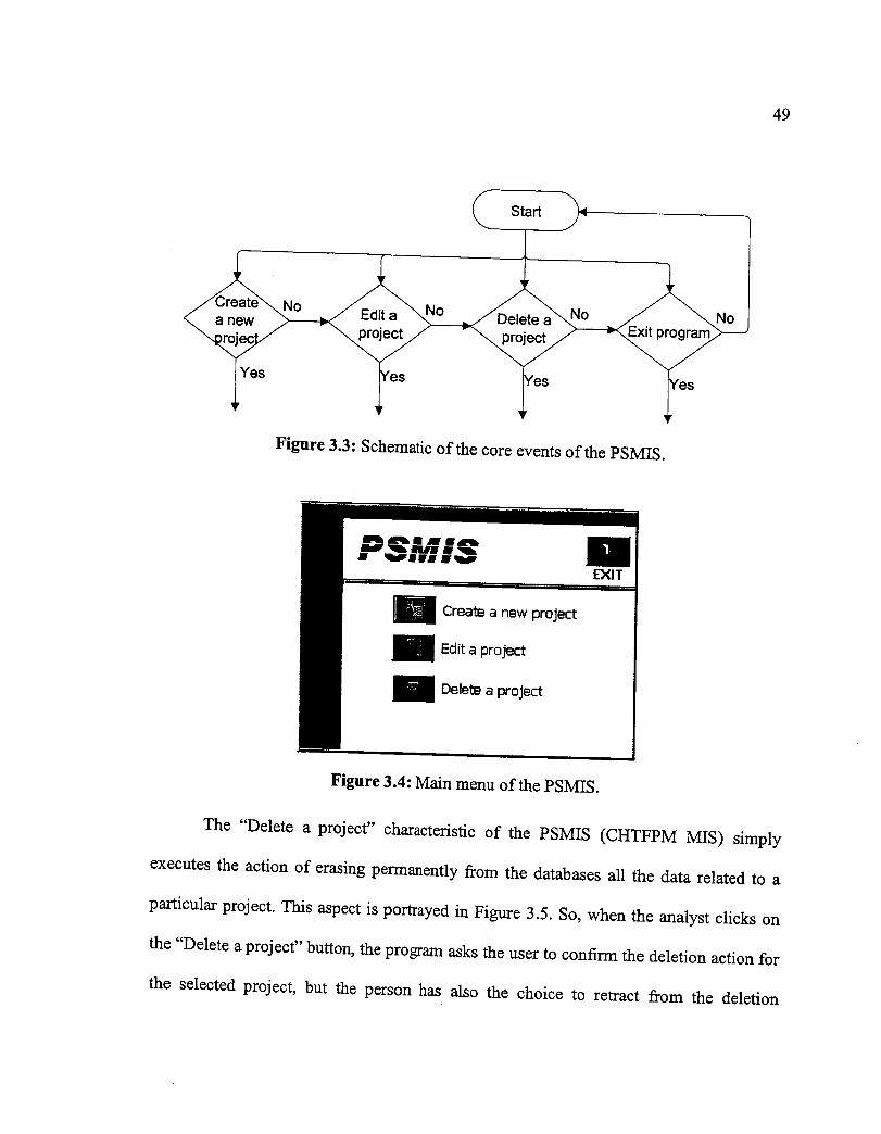
49
Start
Figure 3.3: Schematic of the core events of the PSMIS.
I Creai_a new project
Edita project
Oelebea project
EXIT
Figure 3.4: Main menu of the PSMIS.
The "Delete a project" characteristic of the PSMIS (CHTFPM MIS) simply
executes the action of erasing permanently from the databases all the data related to a
particular project. This aspect is portrayed in Figure 3.5. So, when the analyst clicks on
the "Delete a project" button, the program asks the user to confirm the deletion action for
the selected project, but the person has also the choice to retract from the deletion

5O
process, as seen in Figure 3.6.
Start )
No
Select
project
No
Erase
-- projectdata
Figure 3.5: "Delete a project" event of the PSMIS.
Protect Number:
Project Name: ICalibration process
Description: IValves calibration
Analyst: IWilliam
Date: I.... 27-Feb-031
This project is about to be deleted permanently!
i.-. i;_/" Abo:_t_
Figure 3.6: Delete window of the PSMIS.

51
Similar to thepreviously depictedelement,theothersimplefactorof theprincipal
eventsis the"Exit program" selection,which is theoptionthatallows theanalystto exit
from theprogram.This featureis verystraightforward andself-explanatory;Figure3.7
illustratesthemannerin which the"Exit program"eventis carriedout.
( Start _
N,
%Exit
program
( n0)Figure 3.7: "Exit program" event of the PSMIS.
The beginning portion of the "Create a project" attribute is essential when
conducting a safety study. The program asks the user to fill out the required fields which
are the "Project ID," "Project Name," "Description" and "Analyst Name" fields. If these
domains are empty the program will not allow the user to continue with the project, as
seen in Figures 3.8 and 3.10.

52
No
[-- EnterI information in
l requiredfields
Start
Requiredfields empty
No
Save file
Yes
Store
information
No =
Figure 3.8: Beginning portion of the "Create a new proj ect" event of the P SMIS.

53
Additionally, Figure 3.9 depicts the information fields of a project that must be
filled when commencing a new project. The "Project ID" feature is the most important
entry, for it is the identification (ID) number/name by which all projects are classified
and recognized. In other words, the project ID is the quality that distinguishes one project
from another and helps preserve the integrity of the system; therefore, the program will
forbid the repetition of a project ID. Figure 3.10 is an example of a message box that the
PSMIS displays when a required field is empty--in this case the "Analyst Name" field
supposedly was not filled out.
m
w
w
m!mm
Proje(t ID
Pro|e(t Name
Description
Analyst Name
DateI27-Feb-03ICalibration process
Valves calibration ..........................
I :isave-new pro|er_t _.i:i i'li rl " i , i " " ' _-
Figure 3.9: New project information screen.
. ,._::_._-_<_.__:';,:_ ..' : '., ..:__-_j
Figure 3.10: Message box indicating that a required field is empty.
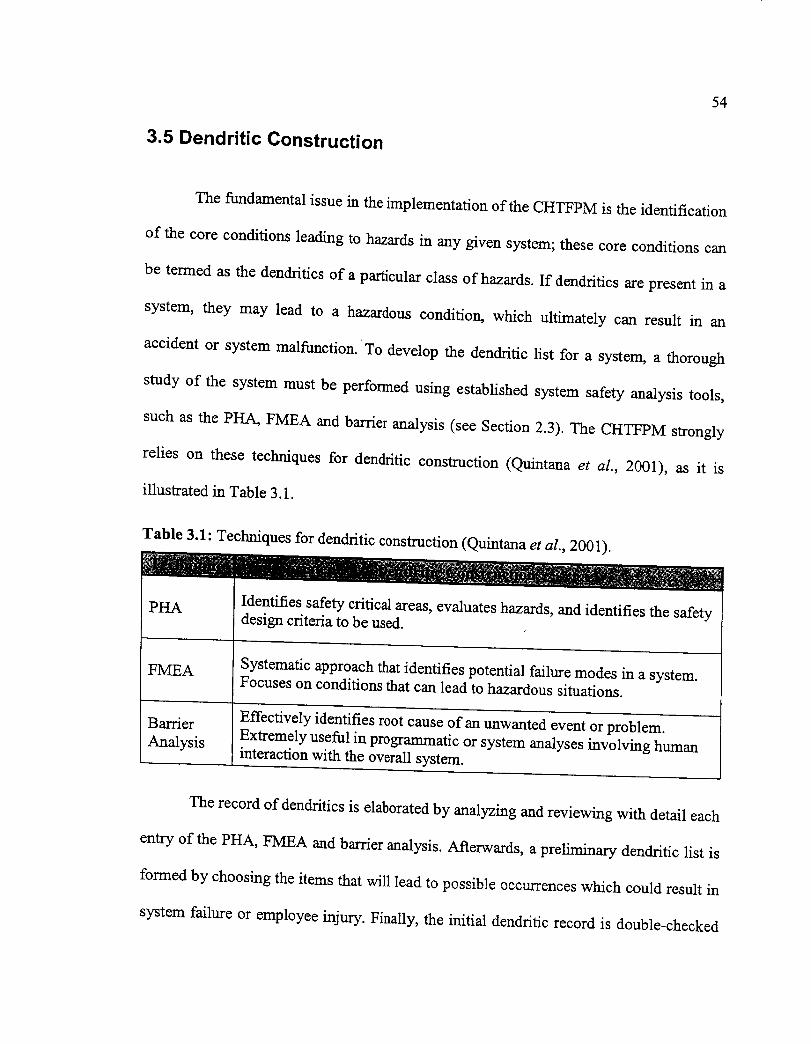
3.5 Dendritic Construction
54
The fundamental issue in the implementation of the CHTFPM is the identification
of the core conditions leading to hazards in any given system; these core conditions can
be termed as the dendritics of a particular class of hazards. If dendritics are present in a
system, they may lead to a hazardous condition, which ultimately can result in an
accident or system malfunction. To develop the dendritic list for a system, a thorough
study of the system must be performed using established system safety analysis tools,
such as the PHA, FMEA and barrier analysis (see Section 2.3). The CHTFPM strongly
relies on these techniques for dendritic construction (Quintana et al., 2001), as it is
illustrated in Table 3.1.
Table 3.1: Techniques for dendritic construction (Quintana et al., 2001).
• w rl
Identifies safety critical areas, evaluates hazards, and identifies the safetyPHAdesign criteria to be used.
FMEA
Barrier
Analysis
Systematic approach that identifies potential failure modes in a system.Focuses on conditions that can lead to hazardous situations.
Effectively identifies root cause of art unwanted event or problem.
Extremely useful in programmatic or system analyses involving human
interaction with the overall system.
The record of dendritics is elaborated by analyzing and reviewing with detail each
entry of the PHA, FMEA and barrier analysis. Afterwards, a preliminary dendritic list is
formed by choosing the items that will lead to possible occurrences which could result in
system failure or employee injury. Finally, the initial dendritic record is double-checked
55
for any repeatingor similar elementsandto enhancethewordingof the items,ensuingin
the concludingversionof thedendriticlist. Nevertheless,thefinal list of dendriticscanbe
modified if more defectsor hazardousconditions are found since undetectedor new
hazards may arise. As indicated by Lee et al. (1998), sometimes as the procedure
advances in an operation, more detailed assessment of hazards has to be performed. All
this process has to be done by the analyst either by hand or by typewriting the
information. This procedure is long and some times tedious; however, it is necessary in
order to identify the dendritics of the system or process.
On the other hand, the PSMIS can accomplish the dendritic construction
automatically and faster. The mode to achieve this course of action is revealed in Figure
3.11, which is the continuation of the "Create a new project" event flowchart in Figure
3.8. Further, to elaborate the inventory of dendritics, the user has two alternatives.
First, the analyst can choose to perform one or all of the analyses forms: PHA,
FMEA or barrier analysis. If he or she did so, then the program will enable the user to
create the dendritic list from the information entered in the forms with the push of a
button called "Import Dendritics."
The second option the end-user has is to create directly the dendritic list without
having to fill out any of the previously mentioned safety sheets; that is, he or she will
specify the dendritics or core conditions that could lead to a hazard according to his/her
own judgment. In addition, the CHTFPM MIS has the capability of allowing the analyst
to modify the list by adding, deleting or editing (rephrasing) dendritics. Moreover, if the
end-user altered the dendritic list and does not like the result of it, the person can reset or
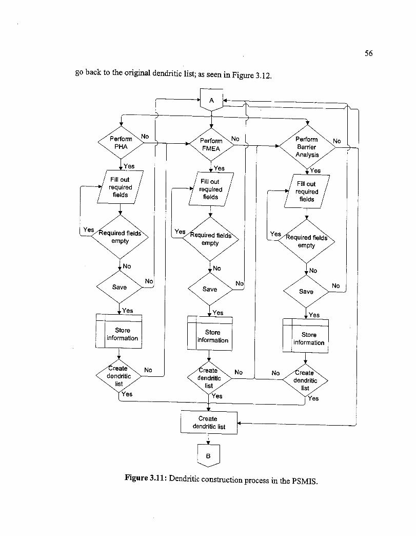
56
go back to the original dendritic list; as seen in Figure 3.12.
Perform
,Yes ,Yes
Fill out Fill out
required requiredfields fields
Perform
Barrier
_'es
Fill out
requiredfields
uired
empty
No
Save
,Yes
Storeinformation
dendritic
"_Yes
uired
empty
No
Save
,Yes
Storeinformation
No No
empty
Save
Storeinformation
dendritic ,_,
dsy?,
Createdendritic list
.4
r
dendritic
"_Yes
Figure 3.11: Dendritic construction process in the PSMIS.
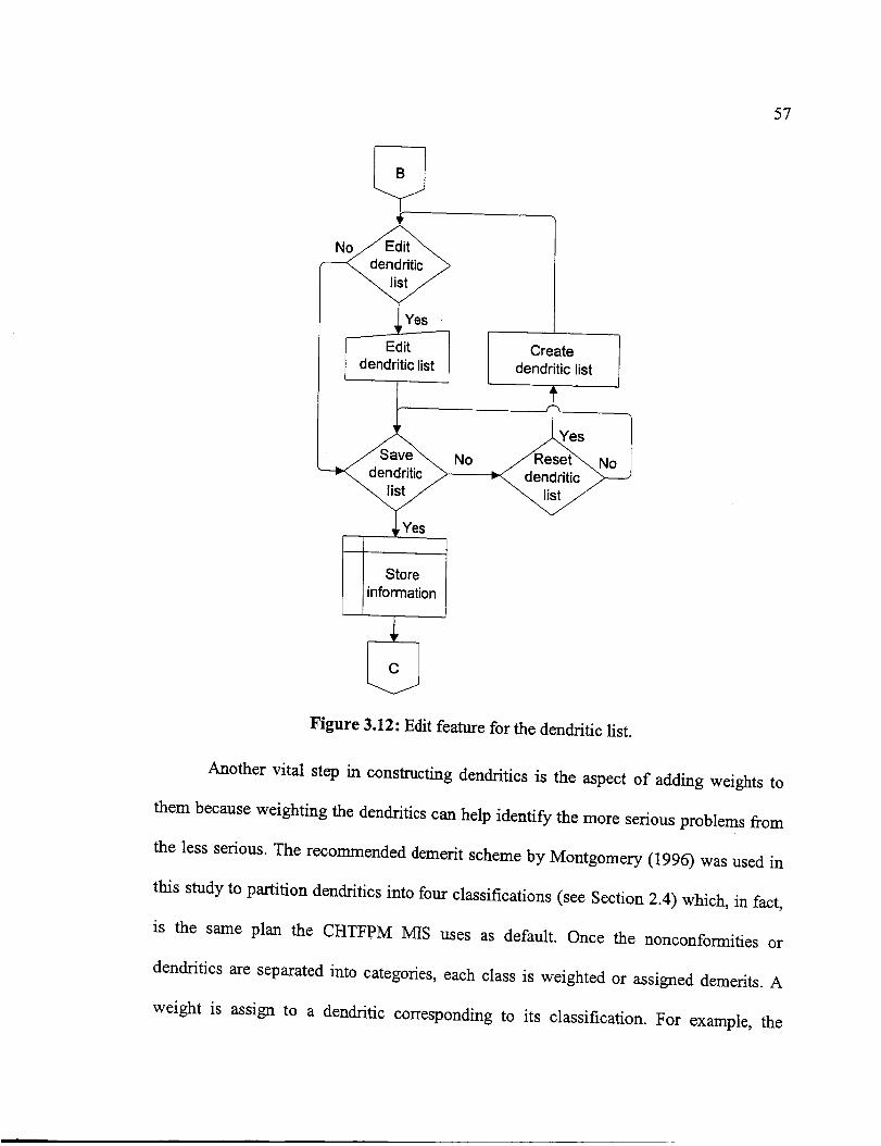
57
dendritic
I Edit
I dendritic list
_rYesi
Storeinformation
No
Create Idendritic list
Figure 3.12: Edit feature for the dendritic list.
Another vital step in constructing dendritics is the aspect of adding weights to
them because weighting the dendritics can help identify the more serious problems from
the less serious. The recommended demerit scheme by Montgomery (1996) was used in
this study to partition dendritics into four classifications (see Section 2.4) which, in fact,
is the same plan the CHTFPM MIS uses as default. Once the nonconformities or
dendritics are separated into categories, each class is weighted or assigned demerits. A
weight is assign to a dendritic corresponding to its classification. For example, the
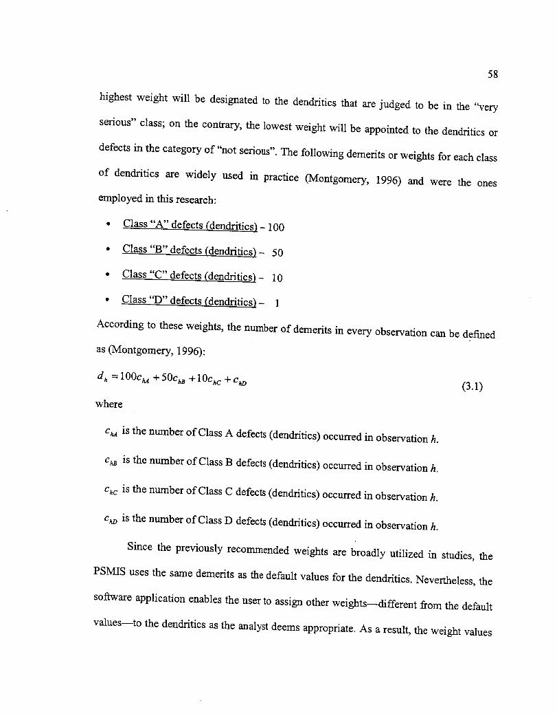
58
highestweight will be designatedto the dendriticsthat arejudged to be in the "very
serious"class;on the contrary, the lowestweight will be appointedto the dendriticsor
defectsin the categoryof "not serious".Thefollowing demeritsorweights for eachclass
of dendritics are widely
employedin this research:
used in practice (Montgomery, 1996) and were the ones
Class "A" defects (dendrifics) - 100
Class "B" defects (dendritics) - 50
• Class "C" defects (dendritics) - 10
• Class "D" defects (dendritics) - 1
According to these weights, the number of demerits in every observation can be defined
as (Montgomery, 1996):
d h = 100Cha + 50ChB + lOChc + Cho (3.1)
where
cha is the number of Class A defects (dendritics) occurred in observation h.
c_ is the number of Class B defects (dendritics) occurred in observation h.
ChC is the number of Class C defects (dendritics) occurred in observation h.
c_ is the number of Class D defects (dendritics) occurred in observation h.
Since the previously recommended weights are broadly utilized in studies, the
PSMIS uses the same demerits as the default values for the dendritics. Nevertheless, the
software application enables the user to assign other weights--different from the default
values--to the dendritics as the analyst deems appropriate. As a result, the weight values

59
of Equation 3.1 will change,correspondingly,to thosechosenby the user.From the
computerprogramstandpoint,the procedureof assigningweights to eachdendritic,after
the dendritic list has been completed,is carried out in the fashion and sequencethat
showsFigure 3.13.
7,:,o!Is/
No
Yes
' Yes 1
_ dendritic
Storeinformation
Figure 3.13: Flowchart for assigning weights to dendritics.
3.6 Safety Sampling
The CHTFPM is a concept of providing safety condition information in a
statistical and economical manner by using the principles of safety work sampling. The

6O
Industrial Engineering Terminology StandardZ94.12 defineswork sampling as "an
application of random samplingtechniquesto the study of work activities so that the
proportions of time devotedto differentelementsof work canbe estimatedwith a given
degreeof statistical validity" (Shell, 1986).A safetysamplingstudyconsistsof a large
numberof observationstakenat randomintervalsor times.In takingtheobservations,the
stateor condition of the objectof studyis notedandconclusionscanbedrawn.
Samplingis theprocessof drawinginferencesconcerningthe characteristicsof a
massof itemsby examiningcloselythe characteristicsof a somewhatsmallernumberof
items drawn from the entire mass,alsotermedasthe populationor universe(Williams,
1978). In general,therearethreecommonmethodsof drawingsamples(Kolarik, 1999):
1. Random Sampling: One or more sampling units selected liom a population
according to some specified procedure. The sample is considered random if the
laws of chance govern its selection. That is, each sampling unit from the population
has an equal chance of being selected. For example, picking an apple from a basket
filled with apples would be a random sample. Each apple has the same probability
of being picked without any apparent preference.
2. Systematic Sampling: A method in which a regularly ordered interval is maintained
between items chosen. An example would be selecting every tenth part that exits an
assembly line.
3. Stratified Sampling: A method which classifies the population units into a certain
number of groups, called strata, and then selecting samples independently from
each group or stratum. The division of the population into strata is usually done in
61
suchaway to reducethe variability of the sampledstatistics.For example,the use
of regular intervalsbetweensamplescanbeapplied,with judgmentalmodifications,
whenit is thoughtthatprocessdisruptionsaremore/lesslikely to occur.
Randomsamplingis the ideal method for samplingbecausea sampletaken at
random from a large group tends to have the samepatternor distribution asthe large
groupor universe.This meansthat in taking randomobservations,the stateor condition
of aprocessunderstudy is notedwith a high degreeof confidenceif the samplesize is
large enough.As a result, from the proportion of investigations,conclusionscan be
drawnconcerningthetotal work activityunderconsideration(Barnes,1957).
In addition,randomsamplingis acost-effectivetool in analyzingasystemsinceit
doesnot require anyadditionalallocationof resources(Quintanaet al., 2001). Random
sampling is also cheaper and faster than a complete observation, also called a census,
because it is usually only a fraction of the group size (Williams, 1978). Consequently, the
random sampling method is by far the most commonly used sampling method in industry
today (Vining, 1998). Therefore, random sampling is the method that the PSMIS will use
to develop a sampling plan. The style in which random sampling will be performed is by
defining the number of subgroups and the number of samples per subgroup, which will
be elucidated shortly.
3.6.1 Groups, Subgroups and Observations per Subgroup
Subgrouping is important because it permits to obtain enhanced statistical
performance in control charts; such enhancement refers to reducing the chance of failing
62
to detect a dendritic or assignablecausein a given systemor process,accordingto
Kolarik (1999). Subgroupingis also valuable becauseit providesa statistical test to
determinewhetherthevariation from subgroupto subgroupis consistentwith theprocess
mean andthe averagevariationwithin the subgroups(GrantandLeavenworth,1996).In
addition, the most obvious rationalbasisfor subgroupingis orderof productionor time
order (Montgomery, 1996),which is anorganizedlist of randomtimesthat arearranged
in sequenceor succession.Therefore,accordingto the rationalepresentedbefore,time
orderis the logical basisthatthePSMISemploysfor datacollection.
The sample size should be chosenin a way that appearslikely to give the
maximum chancefor the observationsin eachsubgroupto bealike (Montgomery,1996).
In other words, the choice of subgroup size should be influenced, in part, by the
desirability of permitting a minimum chance for variation within a subgroup. In most
cases, more useful information will be obtained from, say, five subgroups of 5
inspections than from one subgroup of 25 observations. In large subgroups, such as one
of 25 observations, there is likely to be a much greater opportunity for a process change
within a subgroup (Quintana et aL, 2001).
In many occasions, subgroups of 4 inspections are adequate and sufficient for
deriving reliable conclusions. Subgroup sizes of 4 (+ 1 observations) are extremely
helpful to determine whether or not a group of measurements is statistically
homogeneous, for the possibility of a large variation within a subgroup is considerably
less. Subgroups of size 4 also allow a maximum chance for the subgroups to differ one
from the other (Montgomery, 1996). Since subgroups of size 4 are widely used in

63
practice, the PSMIS recommendsthiscriterion asthe subgrouprange.Nevertheless,the
analystcanchooseanyothersubgroupsize.
For example, if a safety study is to be conductedin an assembly line of a
manufacturing plant for 5 days (assuming each day has one shift of 8 hours), then the
study could be broken down into 5 groups (days) of 8 subgroups (hours) each. The
number of observations per subgroup would be selected by the analyst, say 4. Therefore,
each observation would be represented by a random time in which an inspection would
take place to look for any dendritics present in the system at that moment. This means
that each subgroup would be conformed of 4 arbitrary times (observations).
It is fundamental to mention that the subgroup values are the points plotted in a
control chart in relation to the characteristic of the particular Shewhart control chart being
used. For instance, the p chart plots the fraction of dendritics and the u chart plots the
average of dendritics in each subgroup, but the c char plots the number of defects per
subgroup (Section 3.7 provides a thorough description of this aspect). Developing plots
of subgroup means may appear counter intuitive from a physical perspective; however, it
is essential because it makes a great deal of sense from a statistical point of view since
precision is gained (Kolarik, 1999). In addition, the center line is the process mean, and it
is also computed based on the distinguished quality of the respective attribute (Shewhart)
control chart.
3.6.2 Preliminary Sampling Plan
Initial or introductory samples are indispensable to achieve statistical confidence

64
in a safetystudy. Thereby,it is first requiredto developapreliminary samplingplan in
order to conduct initial observations.This introductory sampling schemeinvoNes
random times, at which the inspectionswill be carried out. The randomtimes canbe
generatedby the CHTFPM MIS or by the analystwith the aid of a programmable,
randombeeperor anyotherdevice,asshownin Figure3.14.
In the event that the first choiceis made,the end-usercanmodify the random
times if thesearenot right. This capabilityis helpful in occasionswhenanarbitrarytime
residesin a momentthatis inappropriate.For instance,if observationswill beconducted
in aproductionline of an industrialplant, it may be possible that a sampling time will be
listed at a period when the operators are scheduled to take a break; therefore, that random
time will fall at an improper instant. If this happens, it is necessary to edit or change that
specific time to a suitable moment (see Figure 3.14); nevertheless, the system analyst can
also disregard that particular time if he or she does not want to correct it.
On the other hand, if the second approach is followed, the user will have to record
the random times whenever the beeper makes a sound and input those times later into a
table that was created by the computer program. That is, the worksheet where the random
times are placed (table for random times) stays vacant--since no times are generated--so
the analyst can enter the beeper times at a later instant. Previous to input the random
beeper times into the computer, the CHTFPM program combines the dendritic list and the
table for random times in order to build a form or sheet for data collection. This form can
be printed to register the data fxom the initial observations if the inspection site is away
from the computer; then such information can be input afterward into the software along

65
with the random beeper times (refer to Figure 3.15). In addition, if the user does not like
the set of random times, for any reason, the individual can create a new list of arbitrary
times, as illustrated in Figure 3.14.
Develop
preliminarysampling plan
Create table for
random times
I Select mode to
generate randomtimes: I=PSMIS,2=other method
No
Edit
random times
comb,neden t,c list & table for
random times
preview of
sampling ]
form J
_<_-. fl rn'_._";n-_'d _- ./_r amndtoh°dtf° res_. _
StoreGenerate information
random times with
the PSMIS ___
_[ saPrndlz/'tng 1
Figure 3.14: Flowchart of preliminary sampling plan.
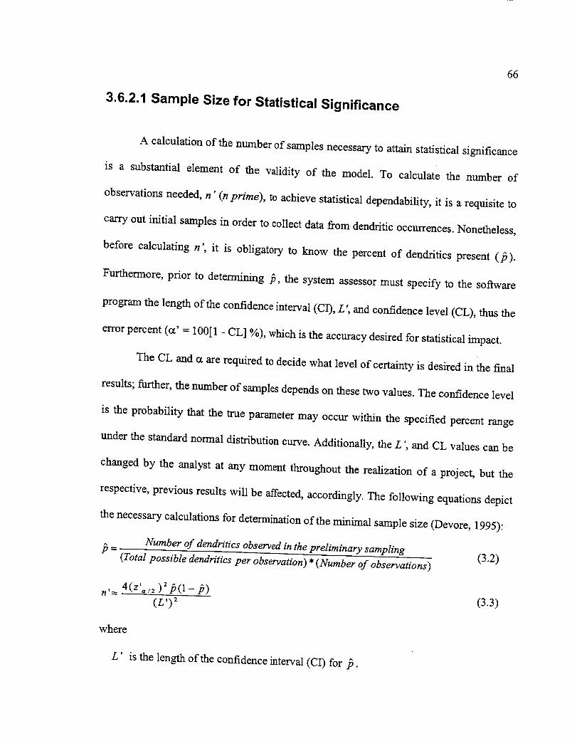
66
3.6.2.1 Sample Size for Statistical Significance
A calculation of the number of samples necessary to attain statistical significance
is a substantial element of the validity of the model. To calculate the number of
observations needed, n' (n prime), to achieve statistical dependability, it is a requisite to
carry out initial samples in order to collect data fi:om dendritic occurrences. Nonetheless,
before calculating n ', it is obligatory to know the percent of dendritics present (/3).
Furthermore, prior to determining _, the system assessor must specify to the software
program the length of the confidence interval (CI), L', and confidence level (CL), thus the
error percent (oc' = 100[1 - CL] %), which is the accuracy desired for statistical impact.
The CL and u are required to decide what level of certainty is desired in the final
results; further, the number of samples depends on these two values. The confidence level
is the probability that the true parameter may occur within the specified percent range
under the standard normal distribution curve. Additionally, the L ', and CL values can be
changed by the analyst at any moment throughout the realization of a project, but the
respective, previous results will be affected, accordingly. The following equations depict
the necessary calculations for determination of the minimal sample size (Devore, 1995):
/3 = Number of dendritics observed in the preliminary sampling (3.2)(Total possible dendritics per observation) * (Number of observations)
n'= 4(z'='2 )2/3(1 -/3) (3.3)(z;') _
where
L' is the length of the confidence interval (CI) for/3.

67
Z'_/2 is the value of the measurement axis for which cc'/2 of the area under the stan(tard
normal curve lies (Devore, 1995).
The previous equations are integrated into the CHTFPM code as well as the
equations for the control limits (view Section 3.7). Therefore, such reckonings will be
performed automatically by the PSMIS. Hence, the analyst can know at what point
statistical significance has been achieved. Figure 3.15 describes the organization and
sequence of this process.
3.6.2.2 Establish Control Limits
In order to establish the safety control limits, a preliminary set of observations
must be performed. This is also done to find out the minimum number of observations or
inspections required to have statistical reliability (n '), based on the desired L' and CL
specified by the analyst. The resulting number of n' is then compared with the acquired
sample size of the preliminary investigation, n, to verify that enough inspections have
been performed. If the required amount of observations has not been reached, the process
of acquiring data should continue until the essential number of samples has been taken.
However, the system evaluator, at any point, can choose to establish the control
limits even if the actual number of samples (n) does not match the number of inspections
needed (n "). In other words, the user can view the actual error percentage, cz, that
corresponds to the actual number of samples, n, that have been taken. If the individual
deems that the real error proportion (cz) is acceptable, then he/she can decide to set up the
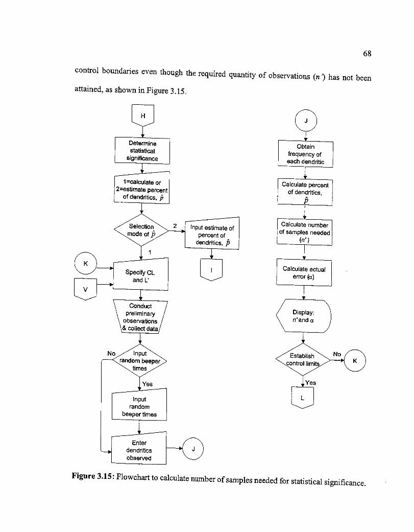
68
control boundaries even though the required quantity of observations (n ") has not been
attained, as shown in Figure 3.15.
statistical
significance
l of dendritics,
_mode ofpJ "]percent of ^
[ denddtics, p
an I L' --/
c°nduct /preliminary /
observations /collect data/
No
I InputI random
J beeper times
___ observeddendn'ticsI -,_/{
Obtain
frequency ofeach dendritic
Calculate percentof denddtics,
Calculate number I
of samples needed(n) I
Calculate actual
error (_)
n'and a
No
Figure 3.15: Flowchart to calculate number of samples needed for statistical significance.

69
In addition, the systemanalystcan alsochooseto specify theproportion/percent
of dendritics, /3, to find the number of samples needed (n). This means that the user can
input an estimate value of /3 before conducting the preliminary observations, but the
subsequent recalculations of/3, if necessary or requested, will be obtained based on the
data gathered from the preliminary data set. If the analyst decides to take this path to
calculate n ', the software will tell the system evaluator the number of samples that must
be taken according to the proportion or percent of dendritics, /3, that he or she predicted,
as observed in Figure 3.16. Then the individual can perform the number of samples
needed for statistical importance.
If the person opts to conduct less observations than the ones stated by the
computer program (based on the approximation of/3 ), the CHTFPM MIS can know the
computed percent of dendritics, /3, in the preliminary data set. With the /3 value, the
PSMIS can also calculate the actual error percentage (eL) that corresponds to the actual
number of observations conducted (n). Thereafter, it is up to the analyst to determine
whether or not to set up the control limits even though the user did not carry out the
required amount of samples (n "); Figure 3.16 portrays this PSMIS procedure when /3 is
estimated. Once all this is accomplished, the control limits can be calculated by the
sottware application (see Figure 3.17) and the analyst can proceed with actual sampling
in the manner described in Section 3.6.3.
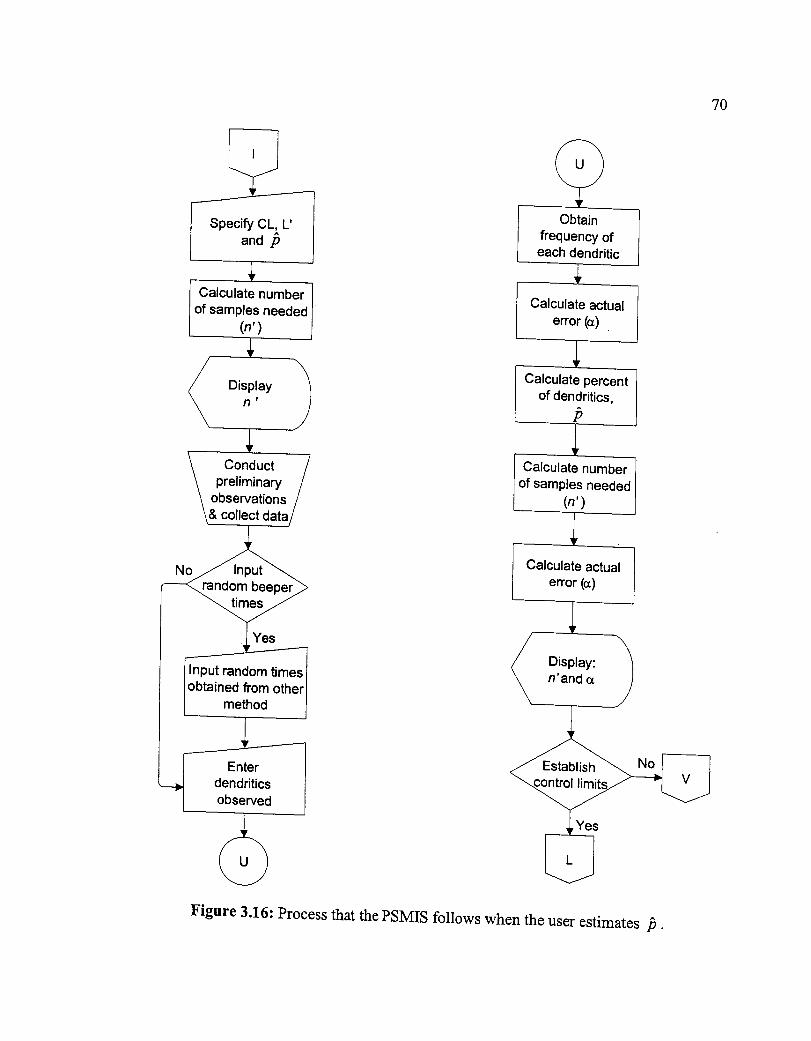
7O
Calculate number
of samples needed(n')
Displayn'
Conduct /
preliminary /observations /& collect data/
No
IInput random timesIobtained from otherI method
nter-_
driticsserved
Obtain
frequency ofeach dendritic
Calculate actual
error (o0
Calculate percentof dendritics,
b
Calculate number
of samples needed(n')
Calculate actual
error (_.)
Display:n'and o_
No
Figure 3.16: Process that the PSMIS follows when the user estimates /3.
3.6.2.3 PSMIS Process to Establish Control Limits
71
The equations for calculating the control limits of all control charts are integrated
in the CHTFPM code as well and are depicted in Section 3.7. Therefore, such reckonings
will be performed automatically by the software system. The CHTFPM MIS executes the
respective computations---center line, LCL, and ULC, etc.---depending on the type of
chart selected. Once the user chooses to establish the control limits, the person needs to
select the type of Shewhart chart that will represent the collected data.
After the preliminary sampling has been terminated, the PSMIS offers the user
four options. The analyst can view the control limits as well as the plotted points for any
of the four attribute control charts--c, p, u or weighted chart--except the EWMA chart
(review Section 3.7.7 for a clarification on this subject). By having the accessibility of
viewing the plotted points of a control chart of the preliminary data, the analyst can
observe if there are any out-of-control points (Section 3.8 elucidates how to deal with
points out of control).
A control chart is constructed graphically by plotting a point or characteristic that
has been measured or computed from a sample (e.g. number of dendritics in subgroup 1)
versus the corresponding sample number (e.g. subgroup 1). The CHTFPM MIS will plot
the chart points according on the attribute chart that is selected. Therefore, even though
the control charts values are plotted in subgroups, each Shewhart chart has a different
way to calculate the subgroup values (refer to Section 3.7 for a detailed explanation of
these characteristics). In addition, Figure 3.17 represents the manner in which the PSMIS
establishes or calculates the center line and control limits in order to make them available

?2
for the analyst to see.
Calculatevalues of: c,center line,UCL & LCL
/Show chart"_(/with values of /\center line, j\UCL &LCL/
2
Calculate
values of:p,center line,UCL & LCL
ith values of /enter line,JCL & LCL/'
I Select chart:
1=c, 2=p, 3=u,4=weighted,
5=Pareto
"3
( _ size of
{ inspection unit
Calculatevalues of: u,center line,UCL & LCL
/Show chart_
(/with values of /\center line, )\UCL &LCL/
_r4
Calculate
weighted II values, center /ltine,UCL_ LCLI
5
Obtain
frequency ofdendritics
Jsho/Dis , y1(/with values of /\center line, ) Pareto\UCL & LCL// .diagram
Figure 3.17: Flowchart for the calculation of the control limits.
in
Additionally, at this stage of the PSMIS, a Pareto diagram is available, as shown
Figure 3.17. This implies that the number of dendritics observed during the
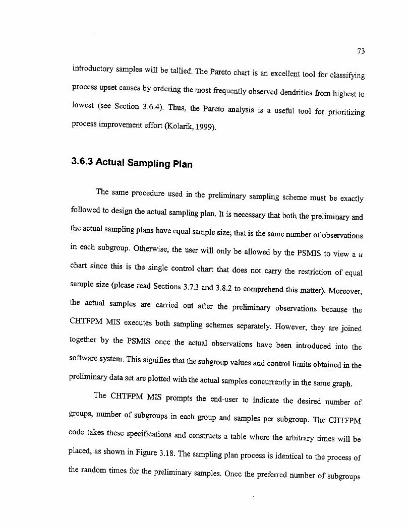
73
introductory samples will be tallied. The Pareto chart is an excellent tool for classifying
process upset causes by ordering the most frequently observed dendritics from highest to
lowest (see Section 3.6.4). Thus, the Pareto analysis is a useful tool for prioritizing
process improvement effort (Kolarik, 1999).
3.6.3 Actual Sampling Plan
The same procedure used in the preliminary sampling scheme must be exactly
followed to design the actual sampling plan. It is necessary that both the preliminary and
the actual sampling plans have equal sample size; that is the same number of observations
in each subgroup. Otherwise, the user will only be allowed by the PSMIS to view a u
chart since this is the single control chart that does not carry the restriction of equal
sample size (please read Sections 3.7.3 and 3.8.2 to comprehend this matter). Moreover,
the actual samples are carried out after the preliminary observations because the
CHTFPM MIS executes both sampling schemes separately. However, they are joined
together by the PSMIS once the actual observations have been introduced into the
software system. This signifies that the subgroup values and control limits obtained in the
preliminary data set are plotted with the actual samples concurrently in the same graph.
The CHTFPM MIS prompts the end-user to indicate the desired number of
groups, number of subgroups in each group and samples per subgroup. The CHTFPM
code takes these specifications and constructs a table where the arbitrary times will be
placed, as shown irt Figure 3.18. The sampling plan process is identical to the process of
the random times for the preliminary samples. Once the preferred number of subgroups

74
and inspectionsper subgrouparespecified,the softwareprogramoffers the analysttwo
optionsto createa samplingscheme.
The first choicethe analysthasis to generatetherandomtimesnecessaryfor each
observationby meansof the PSMIS (seeFigure 3.18). If the user takesthis courseof
action, the computer program will createarbitrary times and wiU place them in the
spreadsheetor tablepreviouslyfabricated.Additionally, just asthedendritic construction
portion of the PSMIS allows the userto changeor edit the dendritic list, the computer
systemalsopermits the analystto modify the randomtimesif thesearenot correct.By
this, it is meantthat in someoccasionsanarbitrarytime mayfall within aninvalid range.
Using againasan illustration the exampleof theassemblyline previouslystated,
it maybepossiblethata samplingtimecouldbe scheduleat aperiodwhentheoperators
areprogrammedto havelunch. Consequently,only thatrandomtime(s)wouldhaveto be
modified or regeneratedto a different,but valid, time insteadof generatingoncemorethe
entirerandomtimesof the samplingplan.
The second alternative the user has to produce random times is by using a
programmable, random beeper or other method. If the analyst decides to pursue this
route, the worksheet, for the random times will remain empty so that the user can input
the random beeper times manually at a later moment. In addition, the evaluator would
conduct an observation whenever the pager alarm goes off; however, the individual must
notice and record the time, at which the observation was taken, so he/she can input that
time afterward in the CHTFPM MIS.
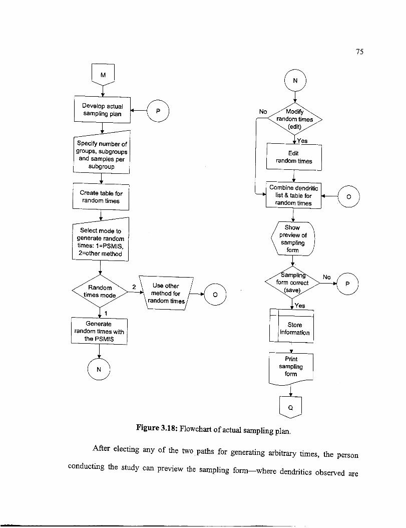
75
I Develop actualsampling plan
Specify number ofgroups, subgroups
and samples persubgroup
Create table forrandom times
I Select mode to
generate randomtimes: 1=PSMIS,2=other method
Generate Irandom times with
the PSMIS
+
No
Edit
random times
___ Combine dendriticlist & table forrandom times
preview of
samplingform
'1 Storeinformation
samplingform l
Figure 3.18: Flowchart of actual sampling plan.
After electing any of the two .paths for generating arbitrary times, the person
conducting the study can preview the sampling form--where dendritics observed are
76
documented--to verify that everythingis correct.If therearemistakes,the end-usercan
goback andmakeanycorrectionsasnecessary. On the contrary, if the sampling form is
correct, it can be printed as a hard copy (view Figure 3.18); thus, observations can be
recorded manually and then transferred or input into the computer program as illustrated
in Figure 3.19.
3.6.4 Pareto Analysis
The Pareto Analysis is art excellent tool for classifying process upset causes by
ordering the most frequently observed dendritics from highest to lowest by means of a
Pareto char or diagram. A Pareto chart is a pictorial representation of a frequency
distribution for categorical data (Devore, 1995). A frequency distribution essentially
provides a count of only the number of observations of a particular characteristic or
category. Each category represents a different type of nonconformity or dendritic. The
categories are ordered so that the one with the largest frequency appears on the far left of
the diagram, then the category with the second largest frequency, and so on (Devore,
1995). Therefore, a Pareto diagram is constructed using rectangles or bars whose heights
are equivalent to the frequencies.
The CHTFPM MIS calculates the cumulative frequency of the dendritics and
arranges them from highest to lowest, so the Pareto diagram can be constructed to portray
which dendritics occur more frequently compared to others. The rank ordering in the
Pareto chart automatically isolates and focuses our attention on the most frequent cause
or dendritics (Kolarik, 1999); thus, proactive measures can be taken more specifically for
77
accident prevention.
Figure 3.19 shows in one of the steps of the process the calculation of the total
frequency of each dendritic. This complete Pareto diagram, which includes the incidences
of both preliminary and actual sampling plans, is only accessible under the "Management
Reports" option (see Section 3.8.1 for a description of this feature). To view the control
charts with the entire observation points plotted (preliminary plus actual samples), the
same previous submenu has to be selected, which is under the "Edit a proj ect" menu.
@@ca ou, /samples & /
ollect data/
No
I Input
I random
I beeper times
dendritics
I observed
Obtain
frequency ofdenddtics
Calculate chart
values: c, p, u,
weighted & Zvalues
Yes
Figure 3.19: Flowchart for calculating total dendritic frequency and entire chart values.

78
3.7 Safety Control Charts Theory
A system or process operating under the presence of assignable causes is said to
be out of control (Montgomery, 1996). Art assignable cause is simply something that is
not common to happen and that is wrong with the process. Assignable causes in the
CHTFPM are the dendritics, or building blocks of hazards. To eliminate an assignable
cause, the process must be fixed or repaired (Levinson and Tumbelty, 1997). Statistical
process control is used to measure the tendency of assignable causes in a process--to
determine if the process is becoming hazardous--, and control charts are employed
extensively for this task (Wise and Fair, 1998).
A control chart is constructed graphically by plotting a point or characteristic that
has been measured or computed from a sample (e.g. number of dendritics in subgroup 1)
versus the corresponding sample number (e.g. subgroup 1). The chart contains a center
line that represents the average value of the quality characteristic corresponding to the in-
control state (Montgomery, 1996). Two outer horizontal lines, called the upper control
limit (UCL) and the lower control limit (LCL), are also shown on the charts. These
control limits are chosen so that if the process is in control, nearly all of the sample points
wiU fall between them.
The manner in which these limits are chosen is by selecting the type of control
chart, thus a distribution, which would best represent the nature of process or system
being analyzed. There are several different types of controls charts (refer to Section
2.5.2.3). Each type of chart has different center lines and control limits. The Shewhart
control charts are also called attribute charts; these charts are preferred in industry
79
becausethey areuniversally applicable,andtherearethreewidely usedattributescontrol
chartsin statisticalprocesscontrol (WiseandFair, 1998).
3.7.1 Control Chart for Nonconformities
There are many practical situations in which it is preferred to work directly with
the number of defects or nonconformities (I._vinson and Tumbelty, 1997). The chart that
lends itself particularly well for this job in the CHTFPM is called the c chart or control
chart for nonconformities. In process control, a nonconformity is a defect in an item or
product. An item may have several quality characteristics that are examined
simultaneously by the inspector. If the item does not conform to standard on one or more
of these characteristics, the item is classified as nonconforming (Montgomery, 1996);
hence, nonconformities represent flaws or defects in a product. In the CHTFPM, the
nonconformities or defects are the dendritics. If a system is said to be nonconforming, it
means that the system is operating under the influence of unacceptable risks or hazards,
which are originated from the dendritics.
A criterion of the c chart is that each inspection unit (e.g. subgroup) must be of
constant sample size. Moreover, this chart assumes that the occurrence of
nonconformities, or dendritics, in inspection blocks of equal sample size is modeled by
the Poisson distribution (Montgomery, 1996). Essentially, this requires that the number of
opportunities or potential locations for dendritics be infinitely large and that the
probability of occurrence of a dendritic at any location be small and constant (Grant and
Leavenworth, 1996).

8O
A c chart is constructed by plotting the number of dendritics or nonconformities
in each subgroup. The parameters of the control chart for the number of nonconformities
per inspection segment are as follows (Montgomery, 1996):
m
Center Line = _ = i=l (3.4)m
UCL = _- + 3-_ (3.5)
LCL = _ - 3_f_ (3.6)
where
i is used as a subgroup or sample index.
c_ is the observed number of defects (dendritics) in sample i (mi).
m is the number of subgroups or samples taken in the preliminary set of data.
is the mean or average of nonconformities (dendritics) per subgroup in the
preliminary set of data.
The 3 is present in the control limit formula because the chart is based on three
standard deviations (3o') fi'om the central value. Thus, the UCL and the LCL will have
approximately 99.73% of all normal observations within their boundaries, since 30
means that approximately 99.73% of all observations should be within these limits
(Vining, 1998). This 3o" control limit on either side of the center line is commonly used to
construct the control charts for work sampling, regardless of its particular use
(Montgomery, 1996).
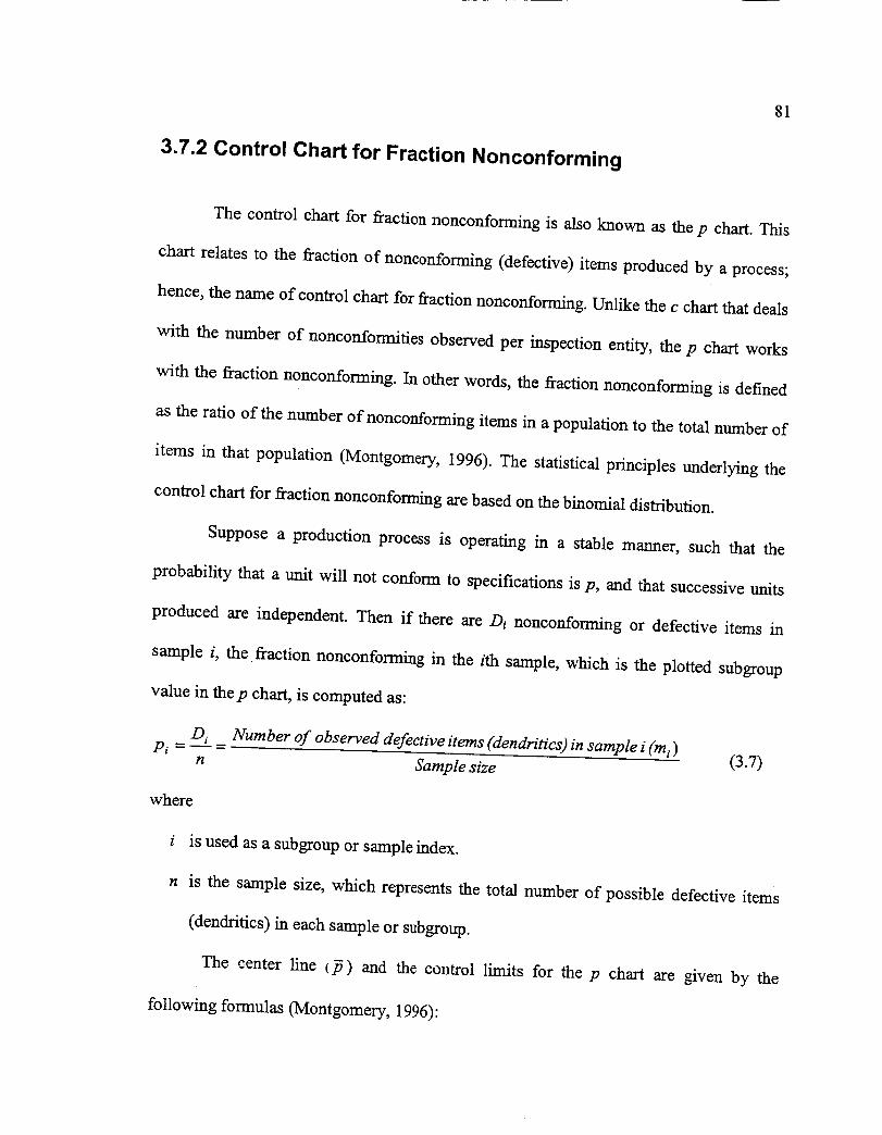
81
3.7.2 Control Chart for Fraction Nonconforming
The control chart for fraction nonconforming is also known as the p chart. This
chart relates to the fraction of nonconforming (defective) items produced by a process;
hence, the name of control chart for fraction nonconforming. Unlike the c chart that deals
with the number of nonconformities observed per inspection entity, the p chart works
with the fraction nonconforming. In other words, the fraction nonconforming is defined
as the ratio of the number of nonconforming items in a population to the total number of
items in that population (Montgomery, 1996). The statistical principles underlying the
control chart for fraction nonconforming are based on the binomial distribution.
Suppose a production process is operating in a stable manner, such that the
probability that a unit will not conform to specifications is p, and that successive units
produced are independent. Then if there are Di nonconforming or defective items in
sample i, the fraction nonconforming in the ith sample, which is the plotted subgroup
value in thep chart, is computed as:
D i Number of observed defective items (dendritics) in sample i (m i )Pi =_=
n Sample size
where
i
n
(3.7)
is used as a subgroup or sample index.
is the sample size, which represents the total number of possible defective items
(dendritics) in each sample or subgroup.
The center _ne (_) mad the control limits for the p chart are given by the
following formulas (Montgomery, 1996):
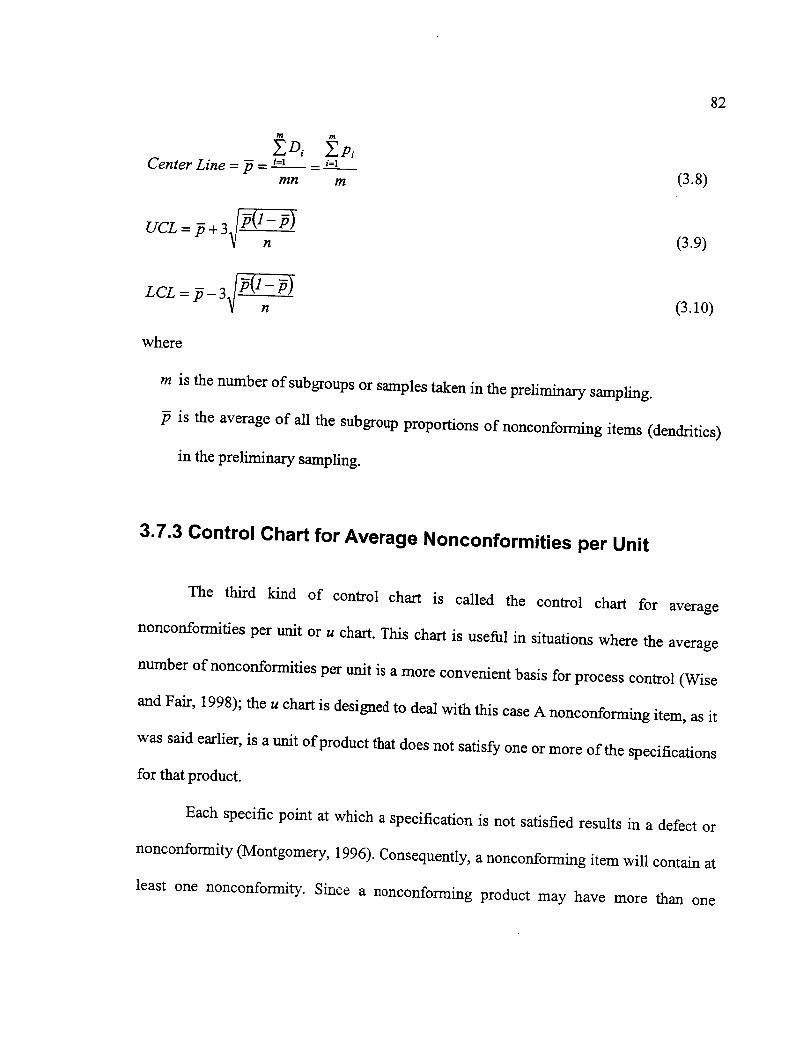
82
m m
Center Line = ff = i=l_!_.__= _=1mn m
(3.8)
UCL= + 34 (lnP'J (3.9)
(3.10)
where
m is the number of subgroups or samples taken in the preliminary sampling.
is the average of all the subgroup proportions of nonconforming items (dendritics)
in the preliminary sampling.
3.7.3 Control Chart for Average Nonconformities per Unit
The third kind of control chart is called the control chart for average
nonconformities per unit or u chart. This chart is useful in situations where the average
number of nonconformities per unit is a more convenient basis for process control (Wise
and Fair, 1998); the u chart is designed to deal with this case A nonconforming item, as it
was said earlier, is a unit of product that does not satisfy one or more of the specifications
for that product.
Each specific point at which a specification is not satisfied results in a defect or
nonconformity (Montgomery, 1996). Consequently, a nonconforming item will contain at
least one nonconformity. Since a nonconforming product may have more than one
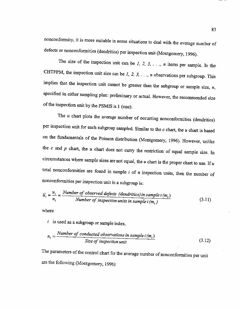
83
nonconformity, it is moresuitablein somesituationsto dealwith the averagenumberof
defectsor nonconformities(dendritics)per inspectionunit (Montgomery,1996).
The size of the inspectionunit canbe 1, 2, 3 ..... n items per sample. In the
CHTFPM, the inspection unit size can be 1, 2, 3 ..... n observations per subgroup. This
implies that the inspection unit cannot be greater than the subgroup or sample size, n,
specified in either sampling plan: preliminary or actual. However, the recommended size
of the inspection unit by the PSMIS is 1 (one).
The u chart plots the average number of occurring nonconformities (dendritics)
per inspection unit for each subgroup sampled. Similar to the c chart, the u chart is based
on the fundamentals of the Poisson distribution (Montgomery, 1996). However, unlike
the c and p chart, the u chart does not carry the restriction of equal sample size. In
circumstances where sample sizes are not equal, the u chart is the proper chart to use. If u
total nonconformities are found in sample i of n inspection units, then the number of
nonconformities per inspection unit in a subgroup is:
ui = u-A-= Number of observed defects (dendritics) in sample i (mi) (3.11)n i Number of inspection units in sample i (m i )
where
i is used as a subgroup or sample index.
Number of conducted observations in sample i (m i) (3.12)
ni = Size of inspection unit
The parameters of the control chart for the average number of nonconformities per unit
are the following (Montgomery, 1996):

Center Line = _ = i=1
m
i=1
(3.13)
84
UCL = _- + 3/2-- (3.14)V ni
LCL=_-3 [ -_(3.15)
3.7.4 Weighted Control Chart
Although the three previously described charts are the most commonly used
Shewhart control charts in practice, there is still one more attribute chart that belongs to
this group: the weighted chart. The aspect of adding weights to the dendritics or
nonconformities, as it was talked about before, can help identify the more severe
problems from the less serious. Moreover, depending on the nature and severity of the
dendritics, it is quite possible for a unit (system) to contain several nonconformities and
not be classified as nonconforming (Montgomery, 1996). For this reason, the weighted
chart is a handy tool in cases of this sort.
As an example, suppose the manufactured items are personal computers. Each
unit could have one or more very minor flaws in the cabinet finish and since these flaws
do not seriously affect the unit's functional operation, it could be classified as
conforming. However, if there are severe defects or too many of these flaws, the personal
computer should be classified as nonconforming, since the flaws would be very

85
noticeableto the customerandmight affect the saleof the unit. In addition, this chartis
alsoassumedto bewell modeledby aPoissondistribution.Mathematically,u is the total
number of demerits in a sample divided by the sample size, which is equal for every
subgroup:
n dDi _ h (3.16)
U i "_n n
where
i is used as a subgroup or sample index.
n is the sample size, which represents the number of observations per subgroup.
Di is the total number of demerits in sample i (m;).
dh is described in Equation 3.1 (Section 3.5).
Since u is a linear combination of independent Poisson random variables, it can be
plotted on a control chart with the following parameters (Montgomery, 1996):
Center Line = _ = 100ff,_ + 50_ B + 10_ c + uz_ (3.17)
UCL = ff + 3_ (3.18)
LCL = _ - 3_ u (3.19)
where
" _ -- 12[(100)2 +(50)2 B+(10)2 c (3.20)
In the preceding equations, uA,us,u c, and u'D represent the average number of Class A,
Class B, Class C, and Class D dendritics, respectively, per subgroup. These values are
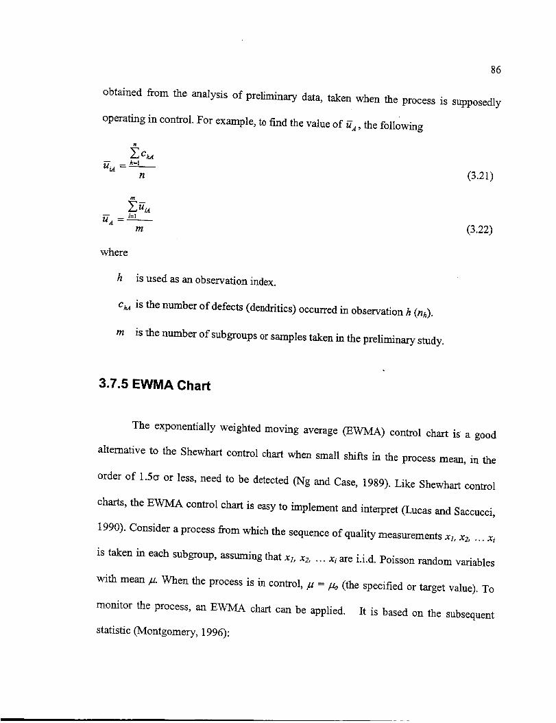
86
obtained from the analysisof preliminary data, takenwhen the processis supposedly
operatingin control.For example,tofind thevalueof uA, the following
tl
_c_
= (3.21)n
where
h is used as an observation index.
c_ is the number of defects (dendritics) occurred in observation h (rth).
m is the number of subgroups or samples taken in the preliminary study.
3.7.5 EWMA Chart
The exponentially weighted moving average (EWMA) control chart is a good
alternative to the Shewhart control chart when small shifts in the process mean, in the
order of 1.5c_ or less, need to be detected (Ng and Case, 1989). Like Shewhart control
charts, the EWMA control chart is easy to implement and interpret (Lucas and Saccucci,
1990). Consider a process from which the sequence of quality measurements xl, x2 .... x_
is taken in each subgroup, assuming that xs, x2 .... xi are i.i.d. Poisson random variables
with mean At. When the process is in control, At =/-to (the specified or target value). To
monitor the process, an EW-N_ chart can be applied. It is based on the subsequent
statistic (Montgomery, 1996):
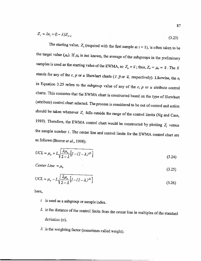
87
Z, = Ax, + (1 - Z)Z,_ 1 (3.23)
The starting value, Zo (required with the first sample at i = 1), is often taken to be
the target value (/.to). If _ is not known, the average of the subgroups in the preliminary
samples is used as the starting value of the EWMA, so Z o = 2; thus, Zo =/1o = 2. The 2
stands for any of the c, p or u Shewhart charts (g, ff or g, respectively). Likewise, the xi
in Equation 3.25 refers to the subgroup value of any of the c, p or u attribute control
charts. This connotes that the EWMA chart is constructed based on the type of Shewhart
(attribute) control chart selected. The process is considered to be out of control and action
should be taken whenever Z i falls outside the range of the control limits (Ng and Case,
1989). Therefore, the EWMA control chart would be constructed by plotting Z i versus
the sample number i. The center line and control limits for the EWMA control chart are
as follows (Borror et al., 1998):
Center Line = _o
here,
i is used as a subgroup or sample index.
L
Z
(3.24)
(3.25)
(3.26)
is the distance of the control limits from the center line in multiples of the standard
deviation (ty).
is the weighting factor (sometimes called weight).
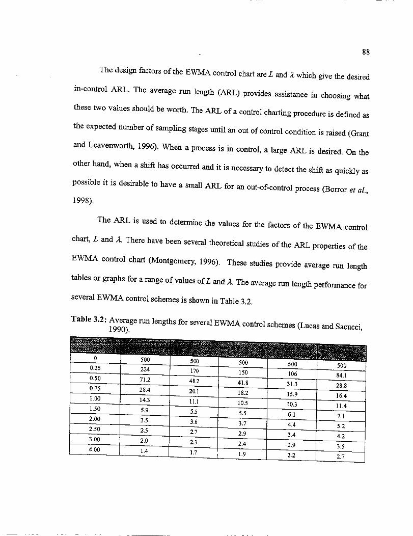
88
The designfactorsof the EWMA control chartareL and _ which give the desired
in-control ARL. The average rtm length (ARL) provides assistance in choosing what
these two values should be worth. The ARL of a control charting procedure is defined as
the expected number of sampling stages until an out of control condition is raised (Grant
and Leavenworth, 1996). When a process is in control, a large ARL is desired. On the
other hand, when a shift has occurred and it is necessary to detect the shift as quickly as
possible it is desirable to have a small ARL for an out-of-control process (Borror et al.,
1998).
The ARL is used to determine the values for the factors of the EWMA control
chart, L and A. There have been several theoretical studies of the ARL properties of the
EWMA control chart (Montgomery, 1996). These studies provide average run length
tables or graphs for a range of values of L and 2. The average run length performance for
several EWMA control schemes is shown in Table 3.2.
Table 3.2: Average run lengths for several EWMA control schemes (Lucas and Sacucci,
1990).
0 500 500 500 500 500
0.25 224 170 150 106 84.1
0.50 71.2 48.2 41.8 31.3 28.8
0.75 28.4 20.1 18.2 15.9 16.4i.
1.00 14.3 11.1 10.5 10.3 11.4
1.50 5.9 5.5 5.5 6.1 7.1
2.00 3.5 3.6 3.7 4.4 5.2
2.50 2.5 2,7 2.9 3.4 4.2
3.00 2.0 2.3 2.4 2.9 3.5
4.00 _ 1.4 I 1.7 t i.9 I 2.2 2.7t I

89
For example, suppose an in control ARL of 500 is desired (the control chart will
plot 500 points before a "false alarm" out of control point is plotted); in Table 3.2, the
various values for L and 2' will give in control ARL's of 500. Additionally, it is also
desired to detect a shift in the safety mean of 1.00 (one standard deviation, or) above or
below the control limits. Using the values for L and 2, in column one, these numbers
should be 3.054 and 0.40, respectively. Therefore, if the system is in control the ARLo is
500 and for detecting a variation in the process mean of lcr the ARL1 is 14.3 (it will take
roughiy 15 subgroups to detect the shift with a point outside of the control limits).
In general, values of 2' in the interval 0.05 < 2' < 0.25 work well in practice, with
2' = 0.05, 2' = 0.10, and A = 0.20 being popular choices (Montgomery, 1996). A good rule
of thumb is to use smaller values of 2. to detect smaller shifts. Further, L = 3 (the usual 3
sigma, 3_, control limits) works reasonably well, particularly with the larger value of 2'
(0.40). However, when 2' is small, ,_ < 0.1, there is an advantage in reducing the width of
the limits by using a value of L between 2.6 and 2.8 approximately, according to
Montgomery (1996).
It is important to point out that when constructing an EWMA chart in the PSMIS,
the person first needs to select a type of Shewhart chart (c, p or u). The reason for this is
because the control limits and the plotted points of the EWMA control chart are
computed based on the center line and subgroup values, respectively, of the selected
attribute chart. This means that the PSMIS creates a c, p or u based EWMA chart,
depending on the analyst's selection. For instance, a c based EWMA control chart cannot
be plotted using the center line and sample values Born the p or u chart. The c based
90
EWMA chart has to be createdusingthe using the meanandsubgroupvaluesof the c
control chart, like comparing apples with apples and oranges with oranges. Moreover, in
order to define the control limits for the EWMA chart, the PSMIS will ask the user to
indicate the L and 2, factors, (notice Figure 3.22). The values of these factors are depicted
in Table 3.2. The sofb_vare program has a help option that provides suggestions to the
analyst about commonly used values for these factors.
3.7.6 Combined Shewhart--EWMA Control Chart
As mentioned earlier, the EWMA performs well detecting small shifts but does
not react to large shifts as quickly as the Shewhart control chart. A good way to further
improve the sensitivity of the control procedure to large shifts without sacrificing the
ability to detect small shifts quickly is to combine a Shewhart control chart with the
EWMA (Borror et al., 1998). The combined Shewhart-EWMA control procedure is
effective against both large and small shifts. This refers that it is possible to plot both the
Shewhart chart and the EWMA chart on the same graph along with the associated control
limits for each chart (Hunter, 1986). This produces one chart for the combined control
procedure which analysts quickly become adept at interpreting.
Of course, the use of either the Shewhart control charts or the EWMA control
chart, or both, in CHTFPM depends upon the nature of the system being analyzed and the
desired protection from unwanted risks and hazards. If the system under observation has
a good track record regarding safety and is relatively stable then, for simplicity, one of

91
the Shewhartcontrol chartsdescribedbeforewill suffice.However,if smallsifts in the
overaUsafetymean causesystemsafetyto degradeto unacceptablelevels,the EWMA
control chartshouldbeused.It is recommendedthat if detectingsmall andlargeshiftsis
desirable,both the ShewhartandEWMA control chartshouldbeusedconcurrently.
3.8 Decision Support Structure of the PSMIS
The CHTFPM M.IS aids the system analyst in making decisions when dealing
with especial issues in a given system or process. These unique subjects are given below:
• Points out-of-control
• Outliers
• Assignable causes
• Trend analysis
• Pattern recognition ,
It is important to highlight at this point in time that most of the whole process of creating
a project is iterative. This denotes that the user can update, change or erase previous
information (wherever the PSMIS allows it) at any moment; consequently, the results
previously calculated will be recomputed or changed. Most important, although the
PSMIS offers recommendations to the system evaluator, the analyst can choose to do
whatever he/she deems more convenient or appropriate.
If a plotted point in a control chart is outside the control limits (out of control), the
system assessor can trace that observation to investigate the reason of that matter. If the
analyst finds out that the cause of such outcome is insignificant, then the person can treat

92
that observationpoint as an outlier, which meansthat the processor systemis not
becoming hazardous.If this is the case,the PSMISwill suggestthe user to erasethe
information (recordeddendritic occurrences)in that particular subgroupand continue
usingthesamecontrol limits for futuresamples.
On thecontrary, if that samepoint turnsout to be anassignablecause(dendritic)
that can jeopardizethe safetyintegrity of the system,then the systemevaluatorhasto
take correctiveactionto fix theproblemthat causedsuchhazardouscondition.Oncethe
fault has been repaired, the analystshould re-establishthe control chart parameters:
center line, UCL and LCL. That is, new control limits must be employed since the
processis no longeroperatingunderthepresenceof hazards.
This connotesthat the sameprocedurefollowed to obtain the control boundaries
for the first time must be repeated.This denotesthat the previouspoints will not be
plotted in the control chartwith the new controlparameters.For this reason,thePSMIS
will propose the user to createa new project in order to preservethe previously
documenteddata.To avoidre-typingthe sameinformationof theoriginal study,theuser
canduplicatethefirst projectand savethenew onewith a differentname, andheor she
will just have to delete the observeddendritics that were registeredin the sampling
sheets.After that, the analystcanusethe samepreliminary samplingplan asthe first one
(original) or createanew oneandbegintheprocessof conductingpreliminarysamplesto
establishthenew controllimits. Oncethis hasbeendone,theusercanproceedto perform
the actual sampling,which will havethe latestcontrol limits obtainedfrom the recent
preliminary dataset.

93
Trending and pattern recognitionarc insightful tools to make inferenceson the
safetystatusof the systemunderobservation.Thesemethodsprovidethe datasourcefor
predictive safety.Theseapproachesarethemost commonusedfor dataevaluationwhen
applying condition monitoring. Thefailure information associatedwith a systemis used
to supply the limits that thetrend andpattern recognitionwill bemeasuredagainstand
what canbe calledanalarmlimit value(Dicquemare,1997).
If the points in a control chartaretruly random,anevendistributionof thepoints
is expectedaboveand below the centerline.However, a control chartmay indicatean
out-of-control condition eitherwhenoneor morepointsfall beyondthe control limits or
when the plotted points exhibit somenonrandompatternor peculiarbehavior,asshown
in Figure 3.20.
.............. ii',Z"....
2 ......2 out of 3 _ o__re p_r_ on or_ side
Figure 3.20: Assignable cause patterns on a control chart (Wise and Fair, 1998)
94
The PSMIS will prompt the analyst to consider the following simple rules
recommendedby Wise andFair (1998)to recognizeor detectanout-of-controlcondition;
hence,takecorrectiveandpreventativemeasures:
1. Pointsbeyondthecontrollimits.
2. Eight or moreconsecutivepointseither aboveor below thecenterline.
3. Fourout of five consecutivepointsin or beyondthe2crlimits (referredto in Figure
3.20asZoneB).
4. Sixpoints or morein arow steadilyincreasingor decreasing.
5. Two out of threeconsecutivepointsin the 3_ region (referredto in Figure 3.20as
ZoneA).
3.8.1 Management Reports of the PSMIS
The management reports are generated from all the information that was included
in the project. In other words, the PHA, FMEA, barrier analysis, dendritic list, control
charts, etc. can be viewed in a defined format or in the form of a report. Since everything
was already calculated (UCL, LCL, dendritics frequency, etc.) by the CH'ITPM code, the
program easily extracts the requested information and displays it in a report fashion,
which can be printed or viewed on the screen. Figures 3.21 and 3.22 illustrate the
flowchart of this process.
Additionally, to display the control charts, the individual has to indicate ;v,hich
chart to view: Shewhart, EWMA or the combined Shewhart-EWMA control chart, as

95
depictedin Figure 3.22.Furthermore,theend-usercancopy thetables,chartsor diagrams
andpastethemin adifferent file or document.
__ Start
Select
project
ViewPHA
NoView No
FMEA Barrier
Yes
Display Display DisplayPHA FMEA Barrier
Analysis
Print Print Print
,Yes Yes .Yes
PHA FMEA Barrier
__ Analysis
No
dendritic .._
_,Yes
( O,so,a,dendritic
list /
Pnnt
I dendritic I
Figure 3.21: Flowchart of management reports (part 1).
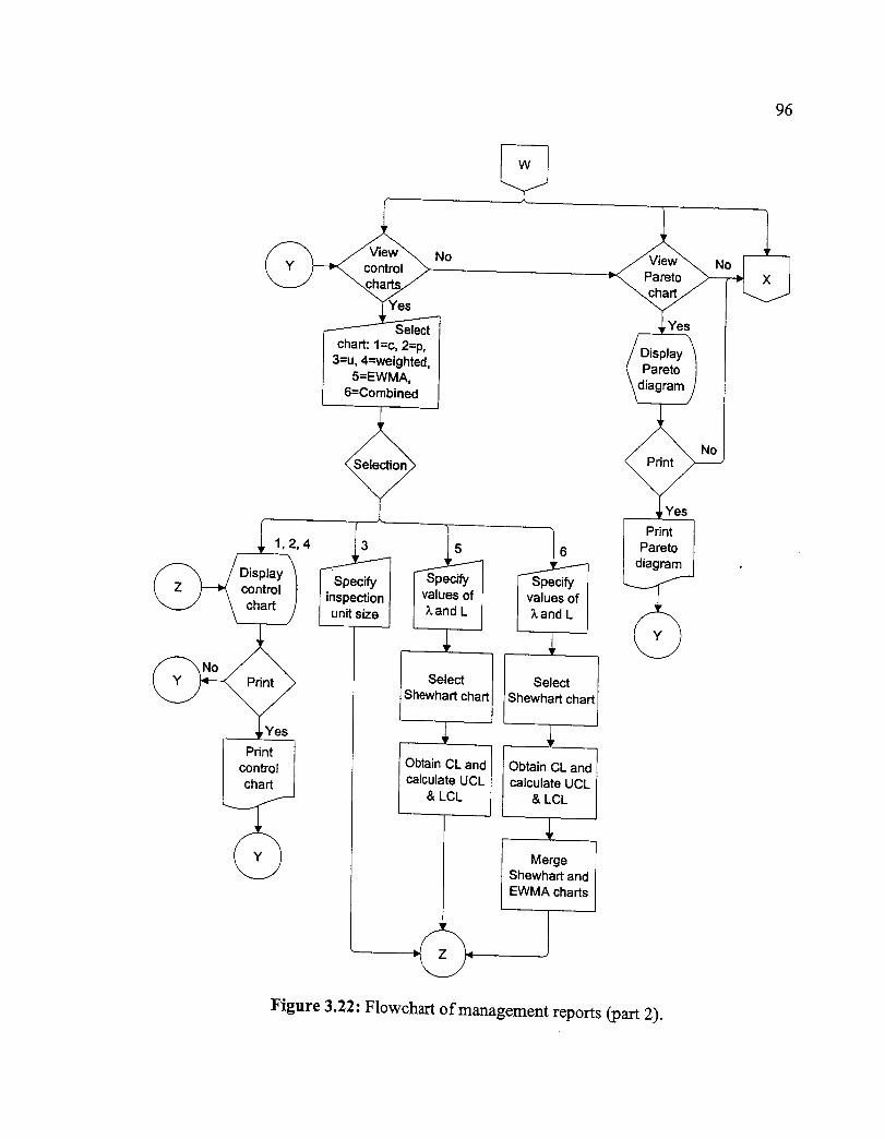
96
No
_-_Pareto
Yes
Pareto
Yes
controlchart
Select r
shewhart chart l
1
Obtain CL and Icalculate UCL J& LCL
Select
Shewhart chart ]
1
Obtain CL and Icalculate UCL P& LCL
Merge /Shewhart andEWMA charts
Yes
rint ]
Figure 3.22: Flowchart of management reports (part 2).
97
Someparts of the project elaboration, as it was said just earlier, are iterative;
therefore, the analyst can make the permitted changes to a project at any point. If this
happens, the existing results associated with the new modifications will be affected
accordingly, but the software application will warn the analyst with regards to the
alterations that are about to take place and will prompt him/her for its consent. If the
individual retracts from its choice, then the changes will not be saved and the current
information will remain the same.
A useful feature of the PSMIS is that it offers the user the ability to view the
collected data in any type of Shewhart control chart if he or she wants to as it is notice in
Figures 3.21 and 3.22. Nevertheless, to realize this operation, the system analyst needs to
go back to the point where the control limits are established, specifically where the
person selects the type of attribute chart (observe Figure 3.17). To return or go to a
locality of interest in the program, the user can simply click on the respective buttons to
continue or advance in the project process until it arrives to the desired location.
3.8.2 Help Screens and Decision Support
The PSMIS will aid or guide the user on how to fill out forms and fields by
providing assistance and advice through help screens. The sections contained in this
chapter include explanations and suggestions to perform certain tasks in the computer
program. All those clarifications or steps that describe how to utilize a function of the
software are summarized in help windows, which are available to the analyst. Many of
these help dialogue boxes are recommendations to the end-user, so that optimum results

98
can be obtained,like in the caseof decidingwhat type of control chart to use. In this
situationthe CHTFPM MIS will offer the user the referencesexplainedin Table 3.3 in
the form of a help screenthat would be accessibleto the systemanalyst.However,the
individual alwayshas the liberty of taking the courseof actionthat is moreconvenient
basedon thedesiredresults,systembeingconsideredandpersonaljudgment.
Table 3.3: Summary of control chart applications in the CHTFPM (Quintana et al.,
2001).
p control chart
c control chart
u control chart
Weighted ccontrol chart
EWMAcontrol chart
Ratio of
nonconforming items
in a population to thetotal number of items
in that populationCounts the total
number ofnonconformities in a
unit or inspection
sampleTracks the averagenumber of
nonconformities perunit
Classifies defects
according toseriousness
Use when detecting
small shifts (1.5¢r or
less) is desired
Use when both small
and large shifts needto be detected
Relative ease of
maplementation,
calculations, andeasy to explain
Relative case of
implementation,
calculations, and,
easy to explain
Relative ease of
implementation,calculations, and
easy to explain
Signals accordingto severestdendritics
Detects small
shifts better thanShewhart control
charts
Provides analysisto detect both largeand small shifts
Does not detectsmall shifts
(<l.5cr) well
Does not detect
small shifts
(<l.5a) well
Does not detectsmall shifts
(<l.5cr) well
Incorrect
classification ofdefect could
cause falsealarms
Does not detect
large shifts aswell as Shewhart
control charts
Short time periodnecessary for
analyst to
become adept at
interpreting chart
CombinedShewhart-
EWMA
control chart
Use to describe
dendritic frequencyin relation to
maximum possibleoccurrences
Use when a countof dendritics is
desired
Use when the
sample size is notconstant
Applicable whensome dendriticsare
more importantthan others
Applicable whensmall shifts in the
safety mean raiseunacceptable safetyrisks
Use ff EWMA
control chart is
being used todetect small shifts
The PSMIS not only provides warnings to the analyst in order to prevent
mistakes, but is also offers the user recommendations in decision making so that he or she

99
can understandand interpret the resultswithout difficulty. For instance,the CHTFPM
MIS offers theusersuggestionsaboutwhich controlchartor distribution is moresuitable
for the type of data collected,as the onesdescribedin Table 3.3 which elucidatesthe
appropriatenessof eachcontrol chartand its recommendedapplication(s).The software
packagedoesthis by meansof informing the userwhat kind of control chart is more
convenient accordingto the responsebeing sought. It is up to the system assessorto
determinewhich control chartwouldbe most advantageousto implementdependingon
the circumstancesof thesystem.
An important aid that the PSMIS provides to the user is when an inspection or
observation screen--where the dendritic occurrences are typed in--is not filled out on
purpose maybe because no dendritics occurred. When this happens, the PSMIS/CHTFPM
MIS will assume that such observation was not conducted and will affect the subgroup
size, hence various calculations and results. In spite of this, the CHTFPM MIS will
prevent the person from committing such mistake by alert him/her that there are some
blank observations. Additionally, the warning message will say how to avoid this
problem. It will tell the user to simply place a 0 (zero) in any of the boxes that are next to
every dendritic in the observation window that was empty. By doing this, the software
program will know that no dendritics were observed in that specific inspection and will
count that observation toward the necessary computations.
If an observation number (screen) was skipped or not filled in either intentionally
or accidentally, the PSMIS will notify the analyst of this issue by displa_.n_g the message
box previously mentioned. Nonetheless, the user can choose to leave unfilled such
100
inspectionnumber.If this is thecase,theCHTFPM computersystemwill inform theuser
with a secondwarning messagethat the only availablecontrol chart will be u chart
because the subgroups vary in sample size. In other words, to view the control charts
other than the u chart, the size of each subgroup have to be the same (review Section 3.7
entirely for sample size restriction). If the analyst does not want to be restricted only to
the u control chart, then the vacant observation screens have to be filled out.

Chapter 4
4. IMPLEMENTATION AND EVALUATION OF THE PSMIS
This chapter describes the implementation as well as the evaluation of the PSMIS
or CHTFPM MIS. As was explained in Section 1.5, two previously NASA validated
projects served as the platform to implement the PSMIS. The results from those two
predictive safety studies were compared with the outcomes obtained using the CHTFPM
MIS to determine the reliability of the results given by the software application.
Moreover, the time and the manpower (persons) required to finish each study
manually was measured against the time and manpower necessary to complete those
same projects when the CI-ITFPM computer program was utilized. Therefore, to evaluate
the reliability and efficiency of this predictive safety soRware package, three key factors
were considered: accuracy of results as well as manpower and time, respectively.
4.1 Introduction
The implementation and evaluation of the PSMIS is outlined in Section 4.2, while
Section 4.3 provides a point by point comparison of the construction of dendritics among
the manual and PSMIS approach. Section 4.4 describes the creation of the sampling sheet
from the manual and PSMIS perspective. In Section 4.5, the development of the sampling
plan in the PSMIS is elucidated, followed by Section 4.6 that reveals how the PSMIS
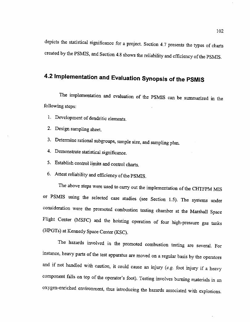
102
depicts the statistical significancefor a project. Section4.7 presentsthe typesof charts
createdby thePSMIS,andSection4.8showsthereliability andefficiencyof thePSMIS.
4.2 Implementation and Evaluation Synopsis of the PSMIS
The implementation and evaluation of the PSMIS can be summarized in the
following steps:
1. Development of dendritic elements.
2. Design sampling sheet.
3. Determine rational subgroups, sample size, and sampling plan.
4. Demonstrate statistical significance.
5. Establish control limits and control charts.
6. Attest reliability and efficiency of the PSMIS.
The above steps were used to carry out the implementation of the CHTFPM MIS
or PSMIS using the selected case studies (see Section 1.5). The systems under
consideration were the promoted combustion testing chamber at the Marshall Space
Flight Center (MSFC) and the hoisting operation of four high-pressure gas tanks
(HPGTs) at Kennedy Space Center (KSC).
The hazards involved in the promoted combustion testing are several. For
instance, heavy parts of the test apparatus are moved on a regular basis by the operators
and if not handled with caution, it could cause an injury (e.g. foot injury if a heavy
component falls on top of the operator's foot). Testing involves burning materials in an
oxygen-enriched environment, thus introducing the hazards associated with explosions.

103
There could be a bum hazard to the operator that could occur during sample unloading
because of molten metal slag. Sample preparation technicians frequently handle cleaning
solvents that require personal protective equipment.
Similarly, the hoisting operation and testing of the HPGTs at KSC entails hazards
related to cumulative trauma disorders such as back or shoulder injuries due to reaching
when hoisting the tanks. In addition, the operators work with pressurized gas cylinders
containing oxygen and nitrogen, so if personnel mishandles or leans heavily on the tanks,
it could release an explosion. Hence, workers are exposed to numerous hazards of
different kinds.
The CHTFPM MIS has two basic features, which are namely the construction of
dendritics, which originate the hazards, of a system and the development of the sampling
study to be conducted in order to detect the presence those dendritics. Based on these two
qualities, the procedure for implementation of the CHTFPM MIS is described in the
following sections which are elaborated using the case studies described in Section 1.5.
4.3 Development of Dendritic Elements
The dendritics for the promoted combustion testing operations at MSFC as well as
the dendritic elements for the testing, preparation and hoisting operation of the HPGTs at
KSC are developed in the following subsections. Determination of the conditions leading
to hazards, the dendritics, is a major step in the development of a project in the PSMIS.
The dendritic focus is on human interaction with the system, as it pertains to both
industrial scenarios. Consultation with system engineers and operators, allowed for the

104
refinementof hazardcriterion.Understandingthesubstructureof the systemsunderstudy
is essentialto recognizepossiblehazards,thus allowed for the inception of dendritic
construction,namelythepreliminaryhazardanalysis.
4.3.1 Preliminary Hazard Analysis
Dendritics are built in part by the fabrication of the Preliminary Hazard Analysis
(PHA), which aids the analyst in identifying and evaluating hazards as well as the safety
design and operations requirements needed to maintain system safety. The PHA is
performed to provide an initial risk assessment of a system. It is based on the best
available data, including mishap data from similar systems. Design controls and other
actions needed to eliminate or control the hazard(s) should be considered or documented.
Hazard HazardCause Effect
Loss of confidenceHuman errorin component
(scheduling) indication
(a)
Hazard Elimination/uirements Control Provisions
Meet minimum calibration Calibration schedulerequirements as specified by reviews and auditsmanufacturer
m_,f_u_ [r_ swtomIs t_ m_mot_ tom.sum t_st_ ¢f_r/_ I
at t_e Mat.a_ Con'Ous't_o_Resea'ch Facllty _ 0n [ C,om[Marshal S¢_.e Fight Center. _ FPIEA
Preliminary Hazard Anah_sis
projectnamoLl_omoted_ Te_g
SafetYlEn_neerk_ Hazard Ebn_at_on/ControlHazardous Condition Hazard Cause Hazard Effect Reguh'9_¢tm Pro_lor=
Figure 4.1: Comparison between the (a) manual and (19) PSMIS approach for the PHA
forms of the MSPC case study.

105
Two PHAs were performedmanually, one for the MSFC study (Appendix A
shows the entire PHA of this project) and the other for the KSC case scenario (see
Appendix H for the entire PHA of this project). Additionally, the corresponding PHAs
were built using the PSMIS. Figure 4.1 depicts the comparison between a portion of the
resulting PHA for the MSFC project by applying the two approaches: manually and via
CHTFPM MIS. In the same way, Figure 4.2 portrays the contrast among two segments of
the PHA, accordingly, for the KSC study.
HazardousConditions
Hazard
Cause
Human Error
1. Non-hazard proof _Failure toelectrical equipment follow SOP)
Hazard Effect
;ire/Explosionresulting in injury_r death to)ersonal and loss3f or damage toflight hardware,Ground SupportEquipment (GSE),and facility.
Safety/Engineering
Requirements
Lock out and tag outall non-hazard proofnon-electrical
equipment
Hazard EliminationControl Provisions
high Pressure Gas Tanks.est work authorization
_rocedures (WAP) containsteps requiring a walk down',overify that all electrical,_quipment has been locked:_utand tagged.
(a)
Hazardous Condition Hazard
,t_man Error q:allure _o
_v SOP)
Figure 4.2: Comparison between the (a) manual and Co) PSMIS approach for the PHA
forms of the KSC case study.
Notice how the two PHAs done by hand (using a word processor program) vary in
format; this is because the analysts involved in the distinct projects have dissimilar

106
interestsor appeals.On the contrary,the PHAs createdby thePSMIShave consistency
throughout.Furthermore,theportionsof thePHAsof thetwo studiesareexactreplicasof
the original analysesforms; this signifiesthatno modificationshavebeenmadeto their
appearanceatthetime of copyingthemto thisproject.This is alsothecasefor theFMEA
andbarrieranalysiswhich arepresentednext.
4.3.2 Failure Mode and Effect Analysis
The PHA, by granting a basic depiction of the hazards and the subsequent safety
design criterion thereof, facilitates the second tool used in dendritic derivation: the failure
mode and effect analysis (FMEA). The FMEA is constructed based on the results
obtained in the PHA. The FMEA is defined as a bottom-up method of identifying the
failure modes of a system and determining the effects on the next higher level. Thereby
tile FMEA form in the PSMIS contains, among others, three fields (or boxes) entitled
"Local Effects," "Next Higher Level," and "End Effects" since there can be more than
one effect caused by a failure. The derived FMEAs (for both projects) consider
human/machine interaction and the possible consequences of such interaction
It is important to mention that there are several techniques to construct an FMEA,
but they are all similar in the sense that they include the same essential information
(fields or headings). Basically, the only variation among the various techniques is that the
titles of the fields are arranged in a distinct way. The following figures show fractions of
the FMEA for both the MSFC and KSC safety studies with their respective FMEA forms
created by the CHTFPM MIS (Appendix B and I give the full FMEA for the MSFC and

107
KSC project,respectively).TheFMEA for theMSFC casestudyis different from theone
for the KSC industrial scenario;moreover,thesetwo FMEA forms are dissimilar from
the onethat the PSMISutilizes. Therefore,Figures4.3 and4.4 illustratethe distinctions
betweenthree typesof FMEA forms.However, it is fundamentalto rememberthat the
FMEAs of eachprojectarean identicalcopyof theoriginal analyses.
Calibration
TechnicianN/A
i
Performscalibration of
assignedequipment(gauges,_transducers, etc)
A. Fails to calibrate equipmentby due dateB. SchedulingD. Inspection of calibrationrecords, visible discrepancy inequipment, etc...E. CalibrateF. VaryingG. yet to be determined
[] Loss of!confidence in
equipmentindication /
operationn Possible failurecause in function /use/operation ofequipment orwstem[] Possible factor
m equipmentdowntime and/orlife expectancy
Possible effectsinclude minor tosevere personnelrisks, systemcomponent failure,system failure
Failure Mode Effect Anab,sis
I¢_llJllct ID _ I_te [ TtllSl:_, N_ 13, 201_
prelectnameIprormmdContemntesrm_goto
Analyst name [l_haet Career
[ De_ar_t_'_Thesw'temlsthec_n_:edcarbusUontesUno
l F_llty IoCa_ or_ I_'_11 SD_r..e R_h_ C_YL'_.
F_lureM_ode/LocalEffert=
II_ _u_rr_t
gg__ _'_ .._,_-._,=--
conmemaungEnd Effects Fault Detectl_rl Provisions ,
(u)
Figure 4.3: Comparison between the ia) manual and (b) PSMIS approach for the FMEA
forms of the MSFC case study.
In some boxes, which are the fields, of the FMEA forms created by the CHTFPM
MIS, the text does not fully fit or is not completely visible. Nonetheless, each box has a
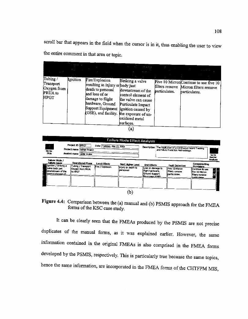
108
scroll bar that appears in the field when the cursor is in it, thus enabling the user to view
the entire comment in that area or topic.
Tubing /Frausport
3xygen fromPRUA toPIPGT
Ignition Fire/Explosionresulting in injury or
5eath to personaland loss of or
5amage to flighthardware, Ground
Support Equipment(GSE), and facility.
Btriking a valve_odyjust_ownstream of the:ontrol element ofthe valve can cause
Particulate Impactignition caused by
the exposure ofun-oxidized metalsurfaces.
Five 10 Micron
filters remove
_articulates.
Continue to use five 10
Micron filters remove_articulates.
(a)
Failure Mode Effect Anal_,sis
_oj_t _ [ser_ proj_-t [ 1GO to Goto
' AMly_
Fak_ _ / CompensatingFailure Cause Operational Phase L_al Effects Next H_hef Level End Effects Fault Dete¢tion prQv_ions '
I_,_/s_a rubing / Trot _/_ IIn_i'yar dea_ = L_s or ,'_r_,_ge_ F_ ZO Micron Contir_ I_ u_ III
i_iV_amtm_ 3,'fgen from PRUA | tper.aorrw, fl_j_t hardware, ,_._ r.m_ r_ ZO M_on M I
II •
(u)
Figure 4.4: Comparison between the (a) manual and Co) PSMIS approach for the FMEA
forms of the KSC case study.
It can be clearly seen that the FMEAs produced by the PSMIS are not precise
duplicates of the manual forms, as it was explained earlier. However, the same
information contained in the original FMEAs is also comprised in the FMEA forms
developed by the PSMIS, respectively. This is particularly true because the same topics,
hence the same information, are incorporated in the FMEA forms of the CHTFPM MIS,

109
correspondingly. The slight disparity is just in the order or fashion that the fields are
structured in each type of FMEA.
4.3.3 Barrier Analysis
The two complete barrier analyses for the MSFC and KSC case studies are
depicted in Appendix C and J, correspondingly. The barrier analyses were performed on
several hazards not identified on the PHA and on the FMEA. Especially those hazards
pertaining to humans were included in these analyses since this type of analysis works
exceptionally well when analyzing human factors affecting system safety or system
components jeopardizing human safety. Again, a section of the barrier analyses of both
projects are shown along with their concomitant PSMIS analyses forms in Figure 4.5 and
4.6 for the MSFC and KSC project, respectively.
Training on general Incorrect posture
Personnel Back Injury safe lab practices used
(a)
Barrier Anah rsis
id_mb_ at the Matw_ContxJStlonRe_rd'tGoto Project name FPromotadComl:x_onTesltng ] iFadltykx:atedonMarshalSl_:e Fl_t Centw.
_mt _, i_,d_ c=_t J '6oto
I _:k Injory i[rraml'_ on generalsa_ lab ect i_:_lureused,
1 ii,, liCo)
Figure 4.5: Comparison between the (a) manual and (b) PSMIS approach for the barrier
analysis forms of the MSFC case study.
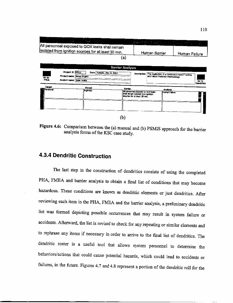
110
Human Barrier Human Failure
(a)
Barrier Anal, sis
_oj,.-t_ _-E'-i D,_.[T.,,_, .,, ,_,20o3 3130to Project .m [SeniorPrOject I
D_cdpUon rThe A_cati_ of a Co_tb_uoJSHazardTr_
iandF_re Ptedct_nMQ_oddo_,
(b)
Figure 4.6: Comparison between the (a) manual and Co) PSMIS approach for the barrier
analysis forms of the KSC case study.
4.3.4 Dendritic Construction
The last step in the construction of dendritics consists of using the completed
PHA, FMEA and barrier analysis to obtain a final list of conditions that may become
hazardous. These conditions are known as dendritic elements or just dendritics. After
reviewing each item in the PHA, FMEA and the barrier analysis, a preliminary dendritic
list was formed depicting possible occurrences that may result in system failure or
accidents. Afterward, the list is revised to check for any repeating or similar elements and
to rephrase any items if necessary in order to arrive to the final list of dendritics. The
dendritic roster is a useful tool that allows system personnel to determine the
behaviors/actions that could cause potential hazards, which could lead to accidents or
failures, in the future. Figures 4.7 and 4.8 represent a portion of the dendritic roll for the

111
MSFC and KSC case studies, respectively, in comparison with the lists made by the
CHTFPM MIS, accordingly. Refer to Table 4.1 and Appendix K for the whole dendritic
list of the MSFC and KSC project, correspondingly.
1. Failure to adhere to SOP
2. Incorrect procedure used to don latex gloves3. Same surface contact (bare hand and glove)4. Personnel wearing dirty latex gloves5. Trash and combustibles not in fire retardant containers6. Test area not in "limited access control"
7. Test cell used for storage8. Personnel limitations for a test cell exceeded (maximum of five)9. Personnel not wearing safety shoes in test area or while moving heavy objects
(a)
Protect Number: _IKEC [ Date: I Tuesday, May13, 20031
Project Name: _romoted Combustion Tesitng I
Description: ITt'_ system is the promoted combustion testing I[chamber at the Material Combustion Research Facility Ilinrat_.d ¢_ Mar_t'uaH_n_t'_. Flinht O=_t_.r.
Analist: _ichael Cametl Ii
_'_i IO DendriEic Weight
___ ll' lllF_uretoad_tosop II ioolI I 2111_°rre_tproced_eusedto_on_texOlo,,e, It _l
=_: I I 4liP-so--elw-_0 di_ylatexOioves--_ i I 5IITrashand co_us_blesnot_ _e reta'dant containers 1[ 1
_i t i 6_lTest area not in 'limited access control" _ .... 10 Ii
_. ii 711Testcellusedf°rst°rage tl 11
:I_ i L_ [personnel limitations for a test cell exceeded (maximum of _VI_]I Z I
Create/ResetDendritics
Figure 4.7:
O)
Comparison between the (a) manual and (b) PSMIS dendritic list of the
MSFC case study.
112
1 gs askew/leaking/corroded.2 Instrumentation calibration not done on regular scheduled intervals.3 Hose/tubing in high-traffic area.4 Personnel not wearin 9 proper Personal Protective Equipment.
_ 5 Over pressurization of HPGTs.6 !Under pressurization of HPGTs.7 !Flow rates exceed preset limits.
8 _emperature exceeds preset limits.9 _eneral cleanliness.
(a)
Dend ritics List
w
ll--....------.
il,
m!
W
W
i,
m
I
I"
l."
im
I
m/-i
P,o_ectN.mbe,:I_Roj 1 o.te:I Tuesda,,_v _3,2oo31Project Name: [Senior Project [
Description: IThe Application of aContinuous HazardTracking and
aibre PredictionMethodobgy,
Analist: I_avierAvalos ]
I Create/ResetDendritics
ID Dendritic Weioht
I _ {Protective coverings askew / _g / corrode,d, II 100[]
/_ II'nstrumentati°n calibration not done on regularscheduled int_lI 50 l
IUtHo-/tubing_tigh-trafficarea. ]{', i' lO/
1 U pe_n_not_._ _operpe_se_ProtectiveEq_koment,Jl I11 lOver pressurization of HPGTs,
i I 6 ilUnder pressur_at_n of H_Ts,
i I 7tl Flow rates exceed preset limits,
l] 8IITemperature exceeds preset limits, I{ lool
Co)
Figure 4.8: Comparison between the (a) manual and (b) PSMIS dendritic list of the KSC
case study.
The PSMIS creates the dendritic list automatically by pressing the "Import
Dendritics" button (see Section 3.5). Additionally, the dendritic list form also has a scroll
bar to view the whole roster of dendritics if they are not visible in the space provided.

113
4.4 Design of the Sampling Sheet
The sampling carried out in CHTFPM is used to check for the presence or
absence of the given conditions, which are the dendritics. However, the sampling sheet is
designed so that it provides the analyst a closer look at the behavior of the system. That
is, it provides the tally marks for the occurrence of each dendritic so that a Pareto analysis
can indicate which one is most significant and causing the system to behave in a
deteriorating manner. This cannot be considered statistically significant, but it provides
an indication of which is the dendritic influencing the system to become hazardous. A
portion of the manual sampling sheet for the promoted combustion testing (MSFC case
study) is shown below in Figure 4.9.
DATE:
1 allure to adhere to the SOP
I
2I
3
4i
5
6
7
8
9
ncorrect procedure used to don latex gloves
Same surface contact (bare hand and latex glove)I
Personnel wearing dirty latex gloves
trash and combustibles not in fire retardant:ontainers
Test area notin "limited access control"
Test cell used for storage
Personnel limitations for a test cell exceeded
maximum of 5 people allowed in test cell area)Personnel not wearing safety shoes in test area orwhile moving heavy objects
COMMENTS:
TIMES:
I '1 I L
I I I
q J
I
I
i
I
Figure 4.9: Sampling sheet created manually for the MSFC project.
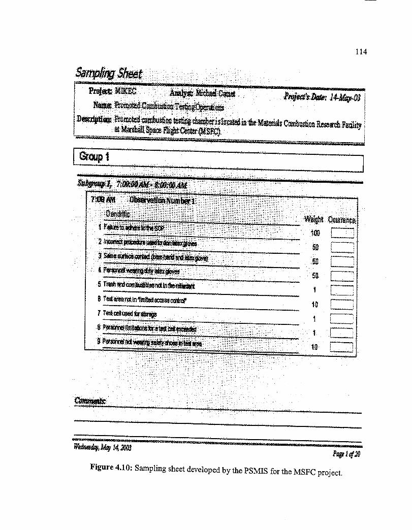
114
............ il .............?i '_''._.;*................. ..........,"_ .......r.......r.........:..........' f'1-"_ .......,,
t0 r
..... " ....... " ._:_ "_' _ _ ._,._"- i._.. :" " i_ .i;_Z_;.;_ ."' " ii_). i ,,;""'"i_ _, ,,, ..........
Figure 4.10: Sampling sheet developed by the PSMIS for the MSFC project.

115
In the sampling sheet for the MSFC study that was done manually, the analyst is
required to note down the time and day when the observation(s) was conducted. On the
contrary, the sampling sheet elaborated by the PSMIS (Figure 4.10) includes the date
when it was printed and the time when the observation should be conducted, so the
analyst does not have to record such information. Therefore, it is strongly recommended
to conduct the necessary observations on the same day the sampling sheet was printed, so
that the printed date will match the observation date.
Similarly, in the sampling sheet for the KSC research study, the system evaluator
has to write down the day and time when the observation will be conducted. Furthermore,
this sampling form (Figure 4.11) does not have a space for commentaries, while the
survey sheet constructed by the CHTFPM MIS (Figure 4.12) does incorporate an area for
comments at the bottom of the page.
Date:
1
2
3
4
5
6
7
8
9
Times
Protective coverings askew/leaking/corroded.Instrumentation calibration not cloneon regular scheduledntervals.
Hose/tubing in high-traffic area.Personnel not wearing proper Personal ProtectiveEquipment.
Over pressurization of HPGTs.
Under pressurization of HPGTs.
Flow rates exceed preset limits.
emperature exceeds preset lim!,ts.eneral cleanliness.
Figure 4.11: Sampling sheet created manually for the KSC project.
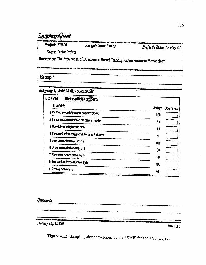
116
i _i ..............................................: ............i.................. t
8_Tem___lm_................... ,r
: : _: _: .
100
50
10
1
100
50
100
Figure 4.12: Sampling sheet developed by the PSMIS for the KSC project.

117
4.5 Rational Subgroups, Sample Size and Sampling Plan
According to the rationale presented in Section 3.6.1, time order was the logical
basis for the data collection in the two studies used to implement the PSMIS. The
promoted combustion testing operations were videotaped over the period of a week. The
videotaped operations were split into 100 subgroups with 4 observations in each
subgroup. Therefore, the sampling plan for this case scenario (MSFC) was constituted by
100 samples of size 4, for a total of 400 observations. The random times corresponding to
the necessary observations for the sampling scheme were generated using a random timer
connected to a time lapse VCR (GYYR, Model Number TLC3168HD).
The mode in which this partition of subgroups was accomplished is described as
follows. The videotaped operations were played back as input into the time lapse VCR. A
random timer that randomly records a set number of clips of certain duration controls the
time lapse VCR. The total time of the videotaped operations was split into 100
subgroups. The random timer was then set to randomly record 4 inspections from each
subgroup. Each random inspection was approximately 10 seconds long to allow adequate
time to check for all 21 dendritics.
On the other hand, the method that the PSMIS uses to achieve the separation of
subgroups is by requesting the user to specify the number of groups, subgroups and
observations per subgroup (see Section 3.6.3 for more details). Before setting up the
sampling scheme, it is critical to keep in mind that the CHTFPM MIS first asks the user
to develop a preliminary sampling plan (see also Section 3.6.3). In the MSFC project, the
preliminary sampling scheme was composed of 10 samples (subgroups), which entailed
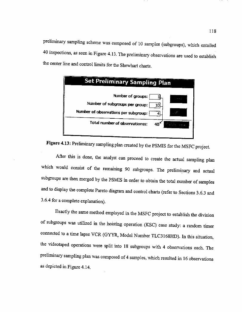
118
preliminary sampling scheme was composed of 10 samples (subgroups), which entailed
40 inspections, as seen in Figure 4.13. The preliminary observations are used to establish
the center line and control limits for the Shewhart charts.
Set Preliminary Sampling Plan
Number of groups:
Number of subgroups per group:
Number of observations per subgroup:
Total number of observationss:
ii • n i i i I I I I iii nil
Figure 4.13: Preliminary sampling plan created by the PSMIS for the MSTC project.
After this is done, the analyst can proceed to create the actual sampling plan
which would consist of the remaining 90 subgroups. The preliminary and actual
subgroups are then merged by the PSMIS in order to obtain the total number of samples
and to display the complete Pareto diagram and control charts (refer to Sections 3.6.3 and
3.6.4 for a complete explanation).
Exactly the same method employed in the MSFC project to establish the division
of subgroups was utilized in the hoisting operation (KSC) case study: a random timer
connected to a time lapse VCR (GYYR, Model Number TLC3168HD). In this situation,
the videotaped operations were split into 18 subgroups with 4 observations each. The
preliminary sampling plan was composed of 4 samples, which resulted in 16 observations
as depicted in Figure 4.14.
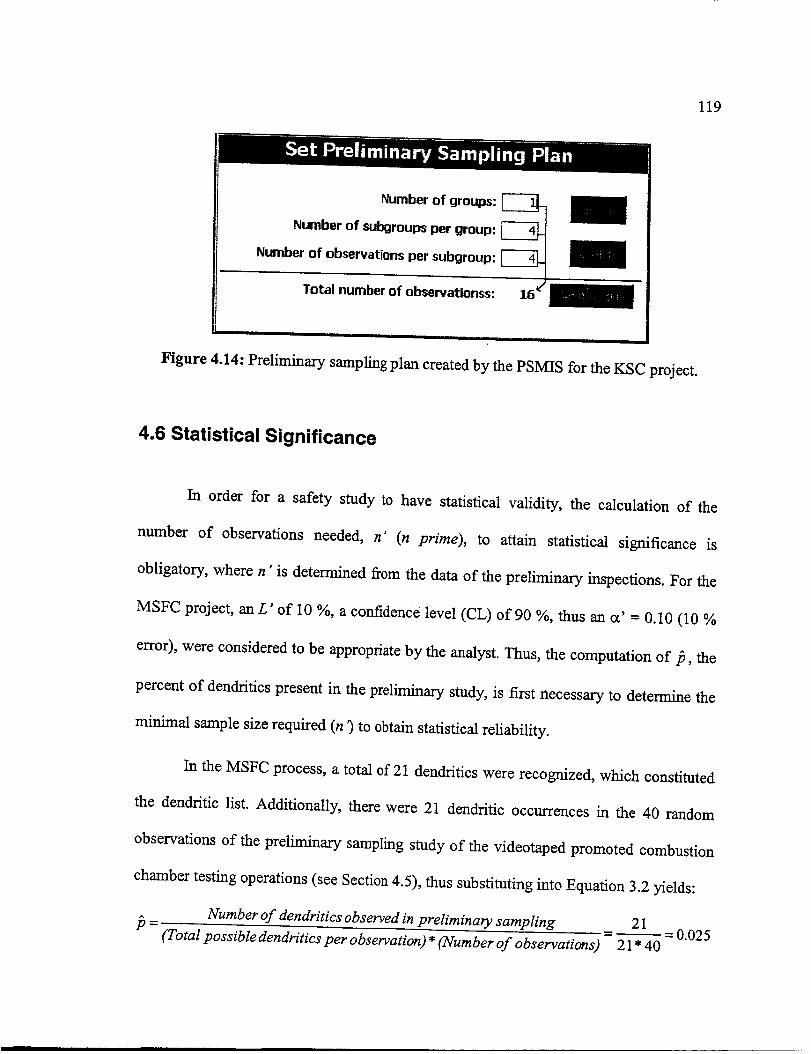
119
Number of groups:
Number of subgroups per group:
Number of observations per subgroup:
Total number of observationss:
I I i ii i iiii i i
Figure 4.14: Preliminary sampling plan created by the PSMIS for the KSC project.
4.6 Statistical Significance
In order for a safety study to have statistical validity, the calculation of the
number of observations needed, n' (n prime), to attain statistical significance is
obligatory, where n' is determined from the data of the preliminary inspections. For the
MSFC project, anL' of 10 %, a confidence level (CL) of 90 %, thus an a' = 0.10 (10 %
error), were considered to be appropriate by the analyst. Thus, the computation of/3, the
percent of dendritics present in the preliminary study, is first necessary to determine the
minimal sample size required (n ') to obtain statistical reliability.
In the MSFC process, a total of 21 dendritics were recognized, which constituted
the dendritic list. Additionally, there were 21 dendritic occurrences in the 40 random
observations of the preliminary sampling study of the videotaped promoted combustion
chamber testing operations (see Section 4.5), thus substituting into Equation 3.2 :_elds:
/3 = Number of dendritics observed in preliminary sampling =_=21 0.025(Total possible dendritics per observation) * (Number of observations) 21 * 40
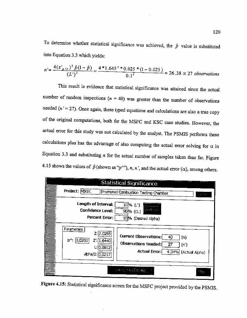
120
To determinewhether statisticalsignificancewas achieved,the /3 value is substituted
into Equation 3.3 which yields:
n'= 4(z'=/2)2/3(1 -/3) = 4"1.645 2 *0.025 *(1-0.025) = 26.38 -- 27 observations(L') 2 0.12
This result is evidence that statistical significance was attained since the actual
number of random inspections (n = 40) was greater than the number of observations
needed (n' = 27). Once again, these typed equations and calculations are also a true copy
of the original computations, both for the MSFC and KSC case studies. However, the
actual error for this study was not calculated by the analyst. The PSMIS performs these
calculations plus has the advantage of also computing the actual error solving for (z in
Equation 3.3 and substituting n for the actual number of samples taken thus far. Figure
4.15 shows the values of/3 (shown as "p^"), n, n ', and the actual error (o0, among others.
Project: INIKEC IIPromoted Combustion Testing Chamber
Length of Interval: l---_% (L')
Confidence Level: F--_-]% (EL)
percent Error: F---_% (Desired Alpha)
m
I
Parameters ]
alpha/2:_
Current Observations: I
Observations Needed: I
Actual Error: I
4o I(n)
27 ](n')
4,34% I (Actual Alpha)
m
Figure 4.15: Statistical significance screen for the MSFC project provided by the PSMIS.

121
Similarly, for the hoisting operation study at KSC, an L' of 10 %, a CL of 90 %,
hence an a' of 10 %, were deemed appropriate by the analyst as well. In addition, 57
dendritic elements composed the dendritic roster. Further, 12 dendritic occurrences were
observed in the 16 inspections comprised in the preliminary sampling data set of the
videotaped operations (view Section 4.5). Replacing into Equation 3.2 gives:
= Number of dendritics observed in preliminary sampling =_=12 0.013(Total possible dendritics per observation) * (Number of observations) 57 * 16
According to Equation 3.3, the number of observations needed to attain statistical
significance (n '), as calculated by the analysts of the KSC project, isthe following:
2n'= 4z"/z/3(1 -/3) = 4 * 1.645 2,0.013 * (1 - 0.013 ) = 14.05 --__15 observations
(L') 2 0.12
In this safety study, the analyst did not calculate the actual error either. Figure
4.16 depicts the _b(shown as "p^"), n, n ', and the actual error (a) values, among others.
I[Seoior ]
Length of Interval: [----_]% (L')
Confidence Level: _]% (CL)
Percent Error: [----_% (DesiredAlpha)
m,
m..
Parameters ]
alpha/2:
Current Observations:[
Observations Needed:[
Actual Error:[
z6 I(n)
is ](n')8.01% 1 (Actual Alpha)
Figure 4.16: Statistical significance screen for the KSC project provided by the PSMIS.
122
The PSMIS rounds up to the next integer the number of inspections needed for statistical
significance. This is done since there cannot be a decimal or fraction of an observation.
4.7 Establish Control Limits and Control Charts
Several control chart procedures were introduced in Chapter 3 (Section 3.7). It is
up to the system analyst to determine which control chart would be most advantageous to
use. This decision can depend on the system being analyzed, data observed, availability
of resources, time, system limitations, desired protection from unacceptable risks or
hazards, desired results, etc.
Once the minimum amount of inspections to possess statistical impact (n) has
been taken, the evaluator can choose to establish the control limits. Nevertheless, if n" has
not been reached, the analyst can still decide to set up the control boundaries if he or she
is satisfied with the actual error percentage, which is provided by the CHTFPM MIS (see
Section 3.6.2.2 for a detailed description).
The first step in developing the control limits is the choice of a Shewhart or
attribute chart, hence an applicable probability distribution. In the research of the
promoted combustion testing operations, the application of the Poisson distribution was
judged to be a good fit for the process. Therefore, the control charts that have an
underlying Poisson distribution are the c and u chart.
As applied to this case study, the c chart was believed to be more suitable to
represent the safety status of the promoted combustion testing system. The c chart will
plot the total number of occurring dendritics (defects/nonconformities) per subgroup. In

123
otherwords, the dendriticswithin the4 observationsof eachsubgrouparesummed,and
that value is plotted. As statedbefore,the preliminary samplesconsistedof the first 10
subgroupswhere 21 dendriticsoccurred.The c chart parameters were generated by
inputting the data of the preliminary study in Equations 3.4 through 3.6, as follows:
m
_c,'
Center Line = _ = i_m
21=- = 2.1 (3.4)
10
UCL = _ + 3_qr_ = 2.1 + 3-_/_ = 6.447 (3.5)
LCL = _- 3q_- = 2.1- 3_ = -2.247 .'. = 0 (3.6)
Here, n is the total number of subgroups (10 samples of size 4). The collected data, or the
number of dendritic occurrences, is positive in nature. Therefore, in the event of a
negative LCL computation, a value of 0 (zero) is assigned.
It should be noted that
out the control limits: UCL
is the process mean or center line which serves to find
and LCL. The control limits calculated by preliminary
samples should be regarded as "trial" control limits, and the preliminary samples should
be examined for lack of control. If there are no out-of-control conditions, then the "trial"
limits can be adopted for future use.
That is why the CHTFPM MIS displays the graph of the preliminary sampling
study, so the user can view if the system or process is stable. Once the end-user verifies
that the system is in control, the assessor can utilize those control limits for the upcoming
or future samples. If there are points outside the limits, the cause(s) for such outcome(s)
should be investigated and addressed (please review Section 3.8 for dealing with out-of-
control points). The fashion in which the PSMIS depicts the values of the control limits is

124
by clicking on the "Seecontrol limits" button (seeFigures4.15and4.16).Thena small
screenappearswherethe analysthasto selectthe Shewhartchart of its preferencein
order to view the respectivecontrol limits, as illustratedin Figure 4.17.The c chart for
the MSFC industrial scenario, constructed from the preliminary data set, is depicted in
Figure 4.18 showing the values of the control parameters---center line, UCL and LCL.
Establish control limitsm
mmmmm
mm
mmm
B
mD
See control limits for:
Figure 4.17: Screen for selecting the type of Shewhart chart control limits.
C chart
_Subgroup --'-- - UCL = 6,447 --.-----Center line = 2.1 - - - LCL = 0 II
1 2 3 4 5 6 7 8 9 10
Subgroup
Figure 4.18: Control parameters of the c chart for the MSFC case study.
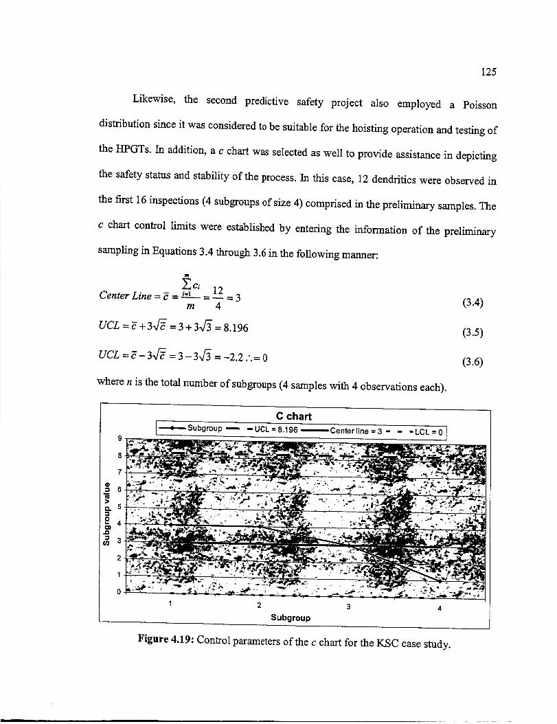
125
Likewise, the second predictive safety project also employed a Poisson
distribution sinceit wasconsideredto besuitablefor thehoistingoperationandtestingof
the HPGTs.In addition,a c chart was selected as well to provide assistance in depicting
the safety status and stability of the process. In this case, 12 dendritics were observed in
the first 16 inspections (4 subgroups of size 4) comprised in the preliminary samples. The
c chart control hmits were established by entering the information of the preliminary
sampling in Equations 3.4 through 3.6 in the following manner:
m
_c_ 12Center Line = _ =/=1 = -- = 3 (3.4)
m 4
UCL = _ + 3.J-_ = 3 + 3._/3 = 8.196 (3.5)
UCL = _ - 3ff-_ = 3 - 3qr3 = -2.2 ... = 0 (3.6)
where n is the total number of subgroups (4 samples with 4 observations each).
Figure 4.19: Control parameters of the c chart for the KSC case study.
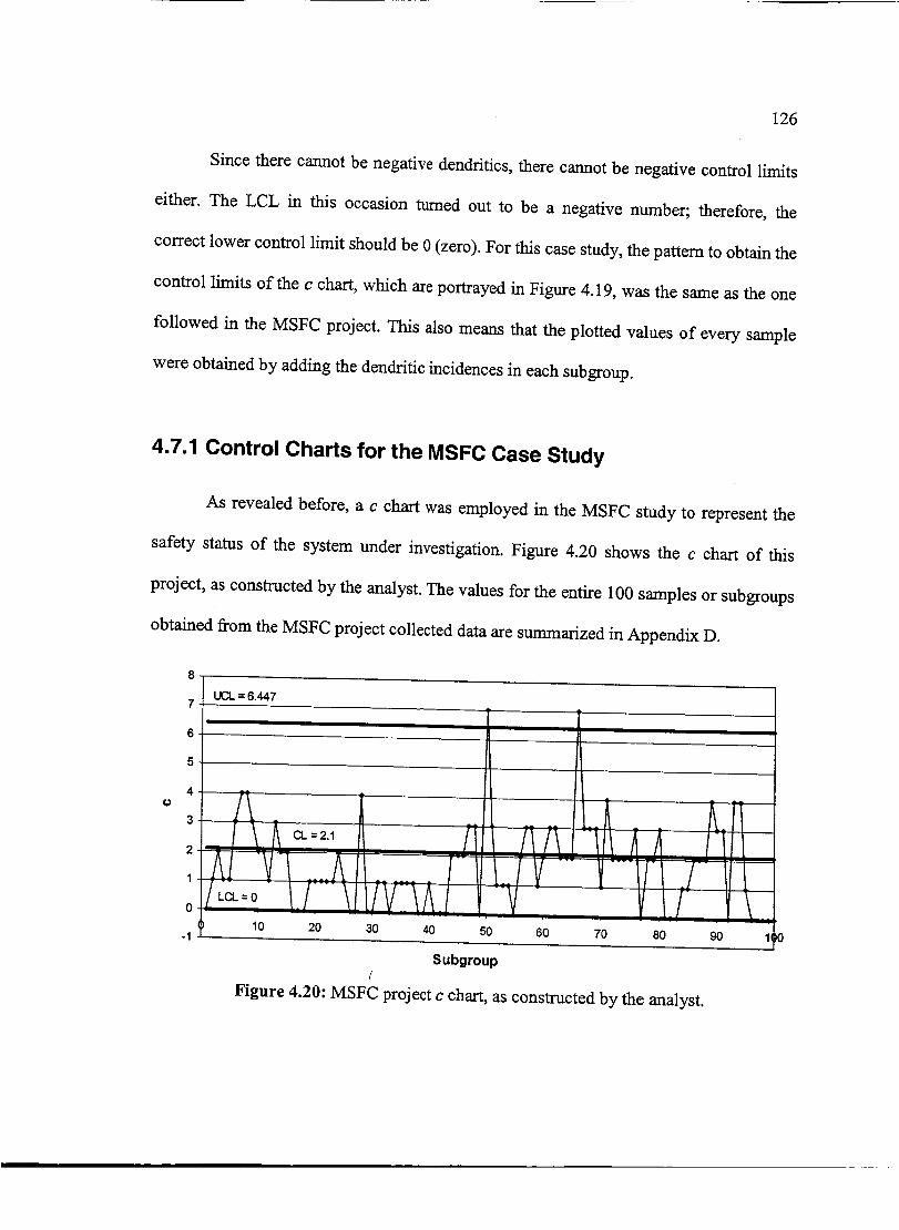
126
Since there cannot be negative dendritics, there cannot be negative control limits
either. The LCL in this occasion turned out to be a negative number; therefore, the
correct lower control limit should be 0 (zero). For this case study, the pattern to obtain the
control limits of the c chart, which are portrayed in Figure 4.19, was the same as the one
followed in the MSFC project. This also means that the plotted values of every sample
were obtained by adding the dendritic incidences in each subgroup.
4.7.1 Control Charts for the MSFC Case Study
As revealed before, a c chart was employed in the MSFC study to represent the
safety status of the system under investigation. Figure 4.20 shows the c chart of this
project, as constructed by the analyst. The values for the entire 100 samples or subgroups
obtained fi'om the MSFC project collected data are summarized in Appendix D.
t_
0
-1
UCL = 6.447
I
3
2
it
A/ V A1_i:::-
[i
l ....
10 20 30 40 50 60 70 80 90
Subgroup/
Figure 4.20:MSFC project c chart, as constructed by theanalyst.
\1 p0
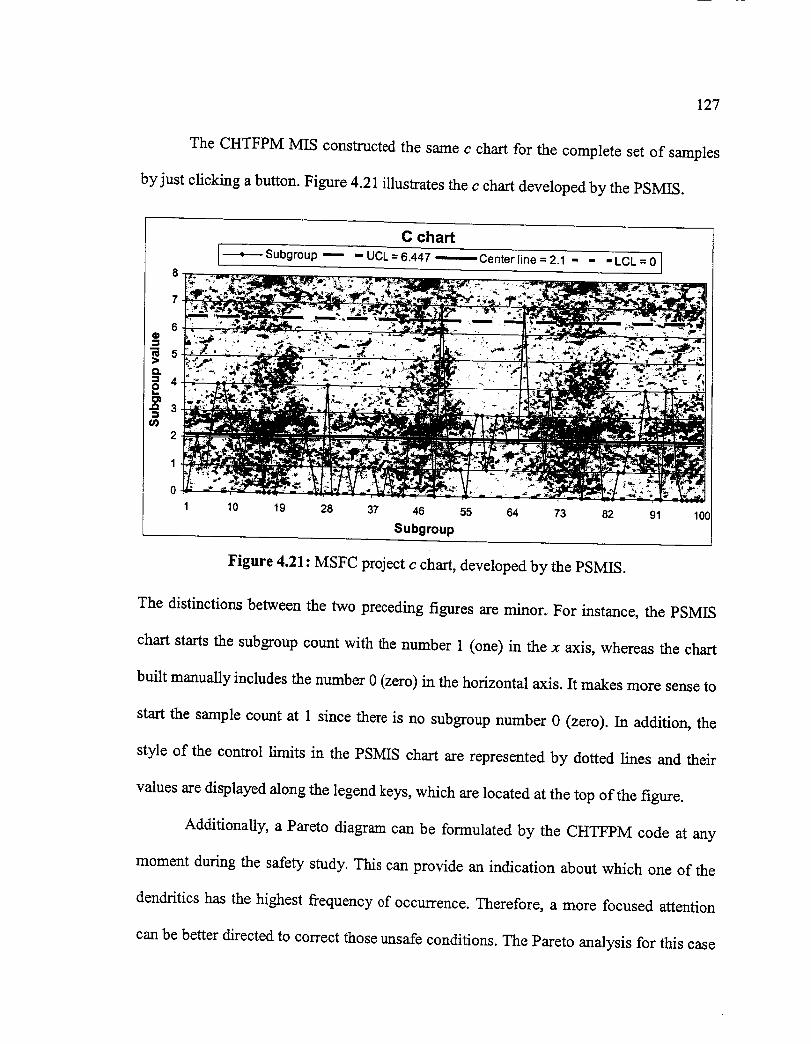
127
The CHTFPM MIS constructed the same c chart for the complete set of samples
by just clicking a button. Figure 4.21 illustrates the c chart developed by the PSMIS.
8
7
6
#,2
1
0
C chart
---*----Subgroup --- - UCL = 6.447 -,------Center line = 2.1 - - - LCL = 0
10 19 28 37 46 55 64 73 82 91 10C
Subgroup
Figure 4.21: MSFC project c chart, developed by the PSMIS.
The distinctions between the two preceding figures are minor. For instance, the PSMIS
chart starts the subgroup count with the number 1 (one) in the x axis, whereas the chart
built manually includes the number 0 (zero) in the horizontal axis. It makes more sense to
start the sample count at 1 since there is no subgroup number 0 (zero). In addition, the
style of the control limits in the PSMIS chart are represented by dotted lines and their
values are displayed along the legend keys, which are located at the top of the figure.
Additionally, a Pareto diagram can be formulated by the CHTFPM code at any
moment during the safety study. This can provide an indication about which one of the
dendritics has the highest frequency of occurrence. Therefore, a more focused attention
can be better directed to correct those unsafe conditions. The Pareto analysis for this case
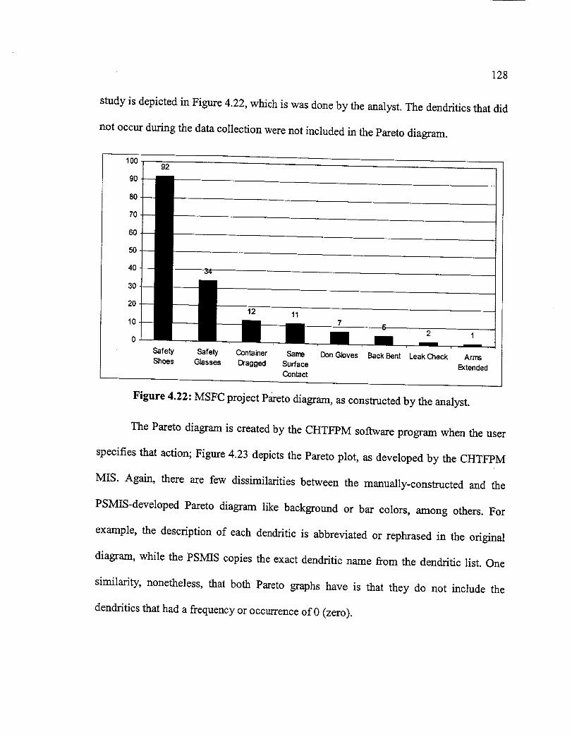
128
studyis depictedin Figure4.22,which is wasdoneby theanalyst.The dendriticsthat did
not occurduring thedatacollectionwerenot includedin theParetodiagram.
10092
9O
80
70
6O
50
40
30
20
10
0
12 11
72 1
Safety Safety Container Same Don Gloves Back Bent Leak Check Arms
Shoes Glasses Dragged Surface ExtendedContact
Figure 4.22: MSFC project P_reto diagram, as constructed by the analyst.
The Pareto diagram is created by the CHTFPM software program when the user
specifies that action; Figure 4.23 depicts the Pareto plot, as developed by the CHTFPM
MIS. Again, there are few dissimilarities between the manually-constructed and the
PSMIS-developed Pareto diagram like background or bar colors, among others. For
example, the description of each dendritic is abbreviated or rephrased in the original
diagram, while the PSMIS copies the exact dendritic name from the dendritic list. One
similarity, nonetheless, that both Pareto graphs have is that they do not include the
dendritics that had a frequency or occurrence of 0 (zero).

129
Pareto diagram
100 L,, .:-£tg-_'_.,arjr_,"._ _- _.,,-,,_-_x.a,-=mb;.=..f. ,, 4. :.._ .-_- _=_,.=a,-,_._.,,-.._,,
t__
60
/ o.i,,
Personnel Technician Container Same Incorrect Back bent Leak Arms full
not w earing not w earing dragged, surface procedure forward checks not extended
safety safety slid or rolled contact used to don performed
shoes glasses latex gloves correctly
Dendritics
Figure 4.23: MSFC project P areto diagram, developed by the PSMIS.
As described in Chapters 2 and 3, not all dendritics are equally impacting the
safety of the system. In situations like this, what is needed is a method to classify
dendritics according to severity, thus weighting the various types of dendritics in a
reasonable manner. The method used to weight the dendritics or to assigned demerits to
them is explained in Sections 2.4 and 3.5. As a result, the dendritics were split into four
classes. Therefore, the dendritics that could cause more serious damage, either to the
system or to the individuals, were clustered in the highest hierarchical category, which is
Class A in this case. The dendritics in the second level of severity were lumped in Class
B, and so forth. The results of this classification, which correspond to the MSFC case
study, are shown in Table 4.1.
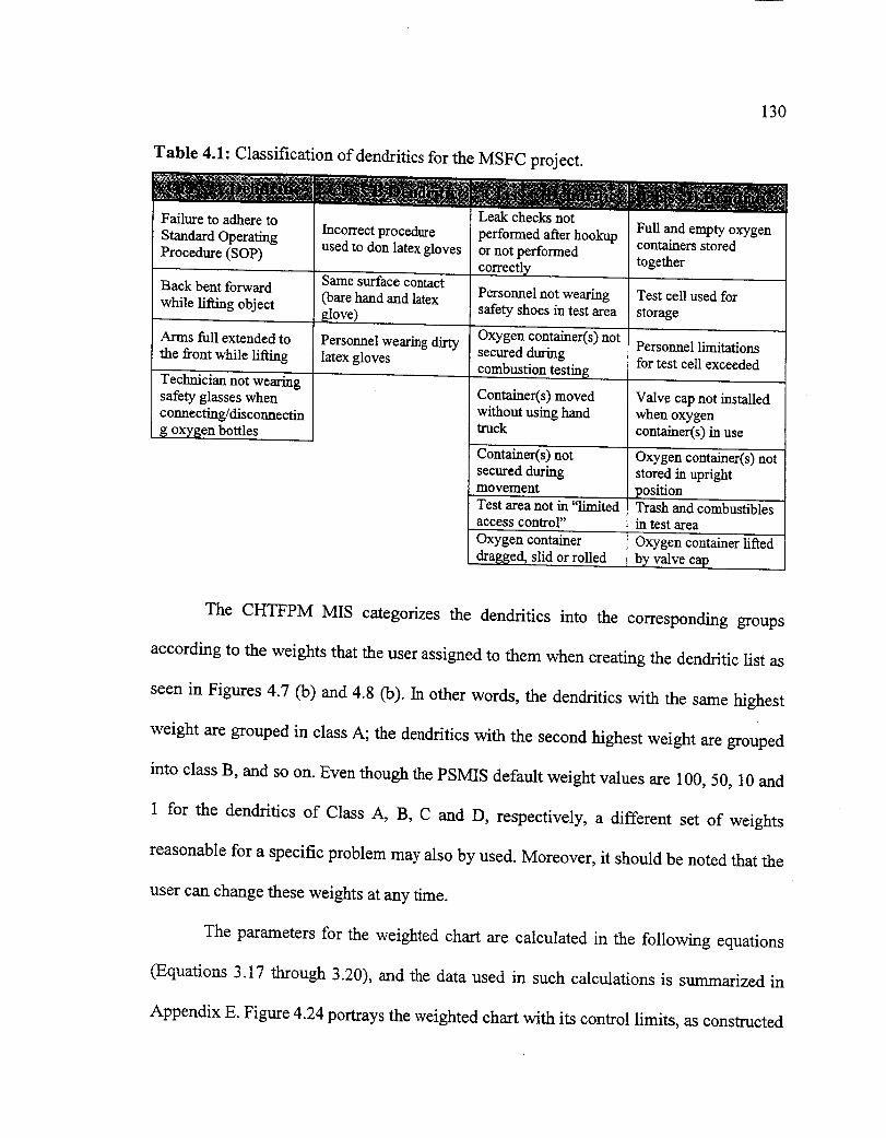
130
Table 4.1: Classification of dendritics for the MSFC project.
Failure to adhere to
Standard Operating
Procedure (SOP)
Back bent forward
while lii_dng object
Arms full extended to
the front while lifting
Technician not wearing
safety glasses when
cormecting/disconnecting oxygen bottles
Incorrect procedureused to don latex gloves
Same surface contact
(bare hand and latex
glove)
Personnel wearing dirty
latex gloves
Leak checks not
performed after hookup
or not performed
correctly
Personnel not wearingsafety shoes in test area
Oxygen container(s) not
secured during
combustion testing
Container(s) movedwithout using handtruck
Container(s) notsecured duringmovement
Full and empty oxygencontainers stored
together
Test cell used for
storage
Personnel limitations
for test cell exceeded
Valve cap not installed
when oxygen
container(s) in use
Oxygen container(s) not
stored in uptight
positionTest area not in "limited Trash and combustiblesaccess control" in test area
Oxygen container
dragged, slid or rolled
Oxygen container lifted
by valve cap
The CHTFPM MIS categorizes the dendritics into the corresponding groups
according to the weights that the user assigned to them when creating the dendritic list as
seen in Figures 4.7 (b) and 4.8 (b). In other words, the dendritics with the same highest
weight are grouped in class A; the dendritics with the second highest weight are grouped
into class B, and so on. Even though the PSMIS default weight values are 100, 50, 10 and
1 for the dendritics of Class A, B, C and D, respectively, a different set of weights
reasonable for a specific problem may also by used. Moreover, it should be noted that the
user can change these weights at any time.
The parameters for the weighted chart are calculated in the following equations
(Equations 3.17 through 3.20), and the data used in such calculations is summarized in
Appendix E. Figure 4.24 portrays the weighted chart with its control limits, as constructed
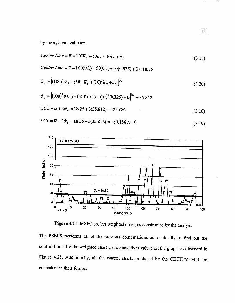
131
by the system evaluator.
Center Line = _ = 100_'_ + 5017B + 10g c + To
Center Line = g = 100(0.1) + 50(0.1) + 10(0.325) + 0 = 18.25
6.= = [(100)2_A +(50)2_ B + (10):_ c +_'_}'_
6.= = [(100) z (0.1) + (50): (0.1) + (10) 2 (0.325) + O]_ = 35.812
UCL = _ + 3d', = 18.25 + 3(35.812) = 125.686
(3.17)
(3.20)
(3.18)
LCL = _-- 3(5-,, = 18.25- 3(35.812) = -89.186 .'. = 0 (3.19)
140
120
100
o
"o 80
6040
20
0
LK1 = 125.686U[ I
0LCL =0
10 20 30 40 50 60
Subgroup
70 80 90 lOO
Figure 4.24: MSFC project weighted chart, as constructed by the analyst.
The PSMIS performs all of the previous computations automatically to find out the
control limits for the weighted chart and depicts their values on the graph, as observed in
Fig,_e 4.25. Additionally, all the control charts produced by the CHTFPM MIS are
consistent in their format.

132
Weighted chart
----*--- Subgroup ---- - UCL = 125.686 --,-----Center line = 18.25 - - - LCL = 0 [140
120
=e lOO
_ 8o
e_ 6o
_ 4o
2O
C
_ _e "_ t ' _ I_= _ _I_"_]F':',_,_ "r ,_, _,L _ - "
10 19 28 37 46 55 64 73 82 91 10C
Subgroup
Figure 4.25: MSFC project weighted chart, developed by the PSMIS.
As mentioned previously in Section 3.7.5, the EWMA control chart is a good
alternative to the Shewhart control chart when small shifts in the safety mean, in the order
of 1.5cr or less, need to be detected. The first step in setting up an EWMA control chart is
determining the parameters L and 1. Using Table 3.2 in Chapter 3, the elected parameters
L and 2. were 3.054 and 0.4, respectively. These values were chosen to detect a shift in
the safety mean of 1.00 with an ARLo of 500 and the ARL_ for an out of control system
of 14.3 (it will take at least 15 samples to detect the shift with a point outside of the
control limits).
The center line for the EWMA chart is also the same as the one from the selected
Shewhart chart, which is the c chart in this case. Utilizing Equations 3.23 up to 3.26, the
plotted points and control boundaries were obtained, respectively. The resulting EWMA
control chart, as constructed by the analyst, is represented in Figure 4.26 (Appendix F

133
encapsulatesthe datausedto constructthis chart),while Figure4.27 showstheEWMA
generatedby thePSMIS.
5 .i
N
4
1
o\
CL =2.1
I
20
-1
10 30 40 50 60 70 80 90 1
Subgroup
Figure 4.26: MSFC project EWMA chart (L = 3.054 and 2 = 0.4), as constructed by the
analyst.
5
4
==
==2
1
EWMA chart
- UCL -.-----,-Center line = 2.1 - - LCL I
37 46 55
Subgroup
64 73 82 91 100
Figure 4.27: MSFC project EWMA chart (L = 3.054 and _, = 0.4), developed by thePSMIS.

134
In both EWMA charts,the control limits arenot shownfor the reasonthat they arenot
constant;that is, eachsamplehas its own set of control limits. However, the control
limits, both the UCL and LCL, tend to reach steady-stateas the subgroupnumber
increases.
In addition, a second EWMA control chart was plotted to demonstratethe
different levelsof sensitivity that canbe attainedusingthis control chart. Supposethe
sameARLo and shift in the safety mean as above are desired but the shift in the safety
mean needs to be detected quicker, say in 10 samples. Using Table 3.2 from Chapter 3,
the values for the parameters 2, and L were 0.10 and 2.814, accordingly. Equations 3.23
through 3.26 equations were also used to construct this EW'MA chart along with the data
provided in Appendix G. Figure 4.28 portrays the resultant EWMA chart, as created by
the analyst.
N
3.0
2.5
2.0
1.5
1.0
0.5
CL=2.1
Figure 4.28: MSFC project EWMA chart (L = 2.814 and 2, = 0.1), as constructed by the
analyst.
0 10 20 30 40 50 60 70 80 90 100
Subgroup

135
The associated pair of the second EWMA control chart, which was developed using the
PSMIS, is shown in Figure 4.29 below.
==z
g#,
EWMA chart
----_-- Subgroup ---= -- UCL ,------Center line = 2.1 '- " - LCL 1
Subgroup
Figure 4.29: MSFC project EWMA chart (L = 2.814 and/t, = 0.1), developed by thePSlVIIS.
A good way to further improve the sensitivity of the control procedure to large
shifts without sacrificing the ability to detect small shifts quickly is to combine a
Shewhart and EWMA chart. These combined control procedures are effective against
both large and small shifts. For example, plotting Figures 4.20 and 4.28 on the same
graph gives the combined Shewhart-EWMA control chart, which is illustrated in Figure
4.30. It should be recalled that the analyst had to do this combination manually (by
manipulating the data) as all the other control charts and calculations shown earlier in this
chapter. On the other hand, the PSMIS performed this combination automatically; Figure
4.31 displays the combined Shewhart-EWMA chart given by the PSMIS.
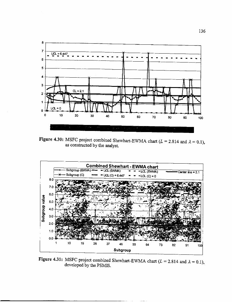
136
v
UCL = 6.447i n i m m m n m I I Im am Im m m • =I mm n m
' A3
_-_L o__-2.,2
oIT=--o/_,J7%0 10 20
mk.
30 40
• lm I i mm m i n m im mm
.3.:.___T:: I _,L.L50 60 70 80 90 1O0
Figure 4.30: MSFC project combined Shewhart-EWMA chart (L = 2.814 and ,,1,= 0.1),
as constructed by the analyst.
Combined Shewhart. EWMA chart
[----e----- Subgroup (EW_ (_-'-_----_ _" _ m Center line = 2.1
Subgroup (C) "_" -UCL(C)=6.447 - - -LCL(C)=O ____
8.0 _=.... r.,a " .. _,_. j,.,..- - ..'- , ._,.,- .,_, ...... _ z,.. ..-,, -_ ..... -:_ -_-,,
-'_. .d. - '7_":"_" ".;_ ' "_ .,"., , .. '. , " ._e-, .,,, , ",,...... . . ,,_ _-" " '_ ;"., _ _,,_,__ ;" ,
=_.of_:.:;. ,_Jl!.: _:...- :. _ ....,_ .,,,_,_:.-_..2_ I
• . _:._ _,'._,. _ ' :: _ j.-_,_ . ._
•" ._,_. - - '_ ' _" ,-_!":". - - " -. a,._._.-,_'_,.._• : ' _- _ . :.., '
1 10 19 28 37 46 55 64 73 82 91 100
Subgroup
Figure 4.31: MSFC project combined Shewhart-EWMA chart (L = 2.814 and )1, = 0.1),
developed by the PSMIS.
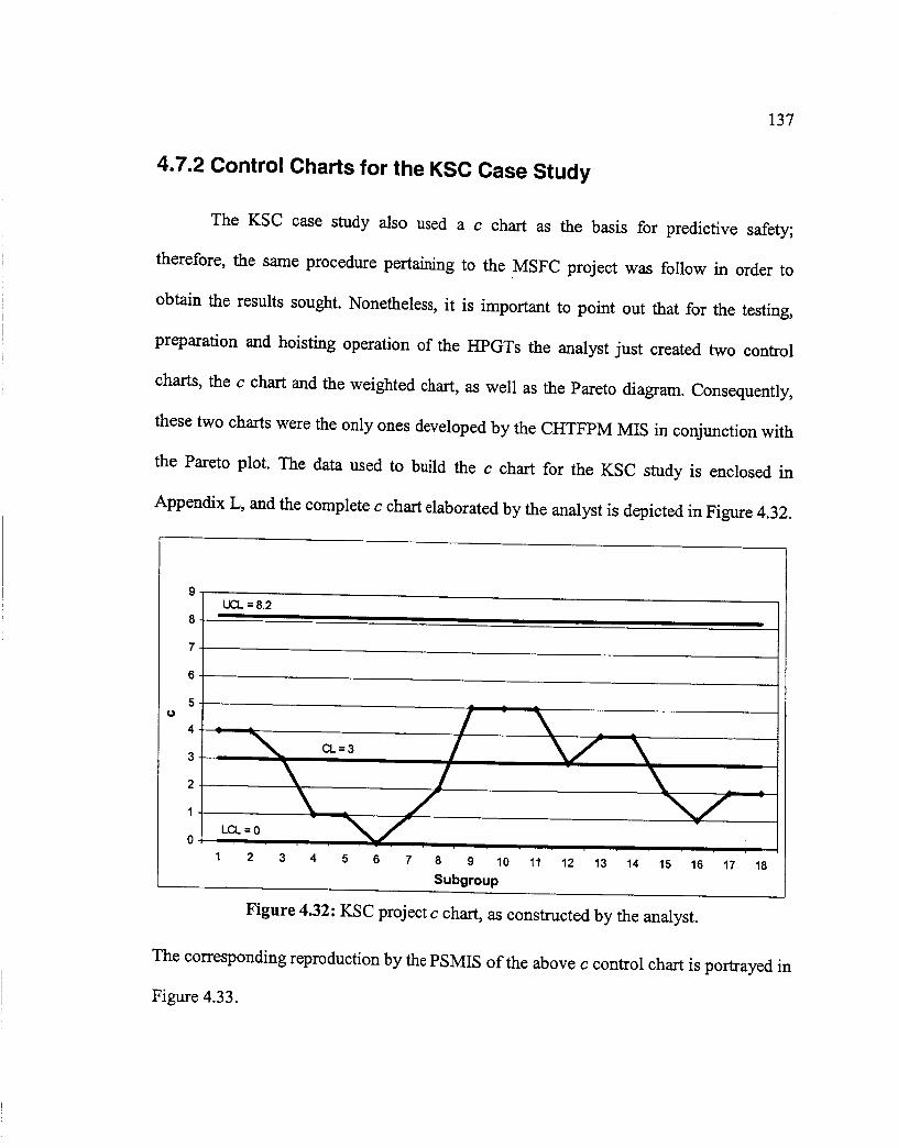
137
4.7.2 Control Charts for the KSC Case Study
The KSC case study also used a c chart as the basis for predictive safety;
therefore, the same procedure pertaining to the MSFC project was follow in order to
obtain the results sought. Nonetheless, it is important to point out that for the testing,
preparation and hoisting operation of the HPGTs the analyst just created two control
charts, the c chart and the weighted chart, as well as the Pareto diagram. Consequently,
these two charts were the only ones developed by the CHTFPM MIS in conjunction with
the Pareto plot. The data used to build the c chart for the KSC study is enclosed in
Appendix L, and the complete c chart elaborated by the analyst is depicted in Figure 4.32.
UCL = 8.2
¢J
JLCL =0
1 2 3 4 5 6 7 8 9 10 11 12 13 14 15 16 17
Subgroup
18
Figure 4.32: KSC project c chart, as constructed by the analyst.
The corresponding reproduction by the PSMIS of the above c control chart is portrayed in
Figure 4.33.

138
.o 4
d3
C chart
_Subgroup _" -UCL=8.2 --=,,,,--Centerline=3 - - -LCL=0 I
Subgroup
Figure 4.33: KSC project c chart, developed by the PSMIS.
A Pareto diagram was also built for this case scenario by the analyst and is
represented in Figure 4.34.
2_
16
1;13
PPE Hose/tubing Reaching SOP
4 4
3
Suspended or Diverted w hUe
moving loads hoisting
Protective
coverings
Figure 4.34: KSC project Pareto diagram, as constructed by the analyst.
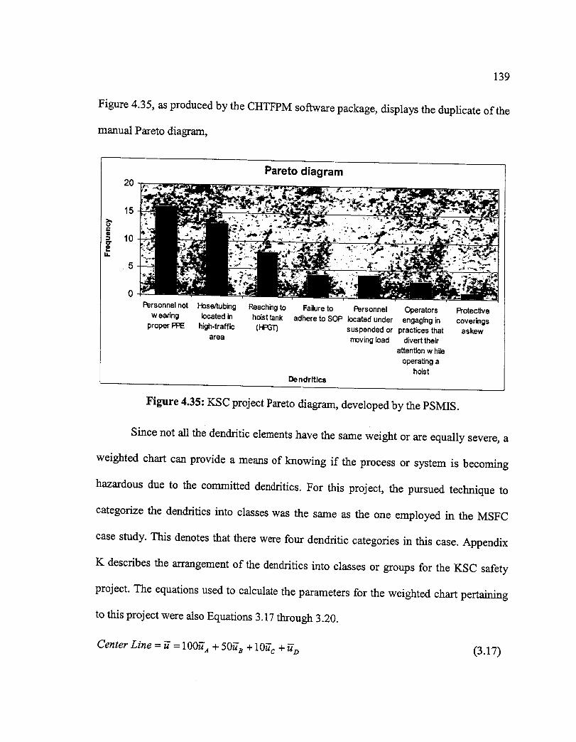
139
Figure 4.35,asproducedby the CHTFPMsoftwarepackage,displaysthe duplicateof the
manualParetodiagram,
la.
20
15 _o
0 __ _y._
Personnel not
w earing
proper PPE
Pareto diagram
Hose/tubing Reachingto Failure to Personnellocated in hoist tank adhere to SOP located under
high-trafflo (HPGT)area
Dendritics
Operators
engaging in
suspended or practices that
moving load divert theirattention while
operating ahoist
Protective
coveringsaskew
Figure 4.35: KSC project Pareto diagram, developed by the PSMIS.
Since not all the dendritic elements have the same weight or are equally severe, a
weighted chart can provide a means of knowing if the process or system is becoming
hazardous due to the committed dendritics. For this project, the pursued technique to
categorize the dendritics into classes was the same as the one employed in the MSFC
case study. This denotes that there were four dendritic categories in this case. Appendix
K describes the arrangement of the dendritics into classes or groups for the KSC safety
project. The equations used to calculate the parameters for the weighted chart pertaining
to this project were also Equations 3.17 through 3.20.
Center Line = _ = 100_" a + 50_"s + 10_ c + U-D (3.17)
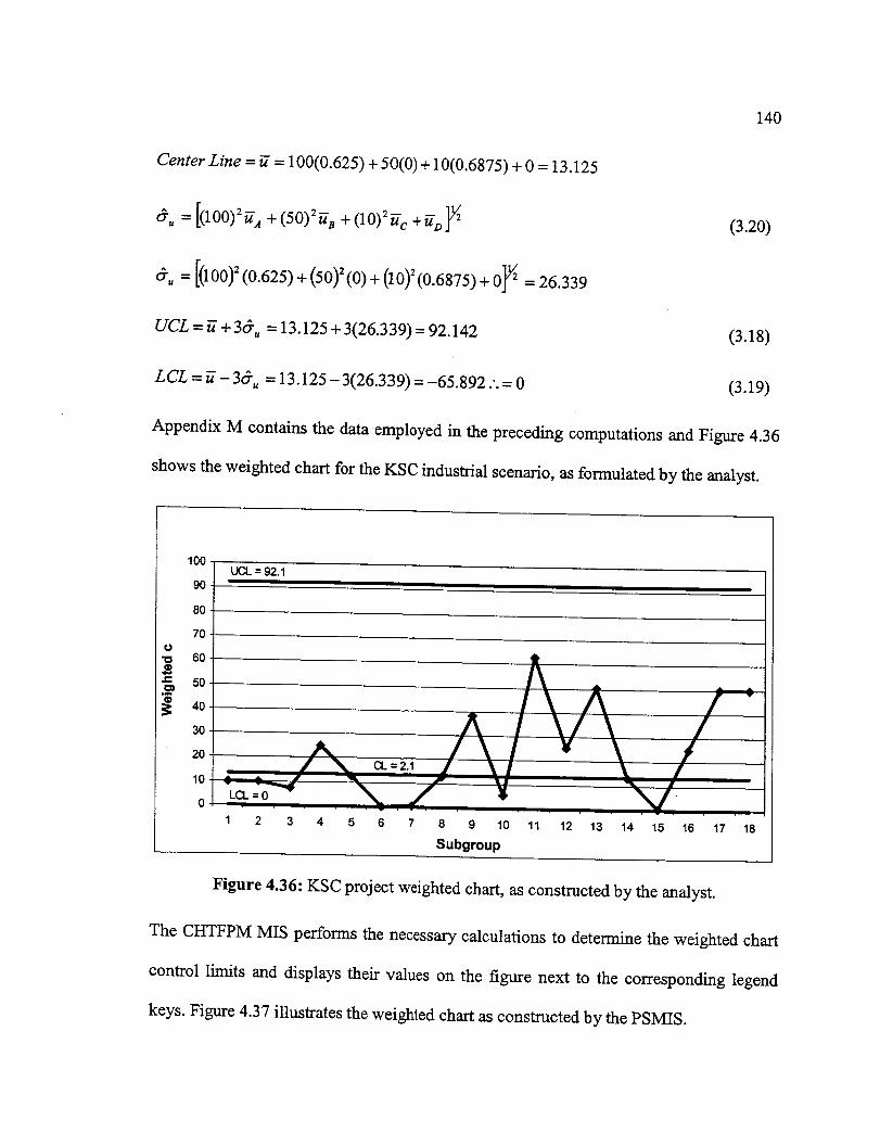
140
Center Line = _" = 100(0.625) + 50(0) + 10(0.6875) + 0 = 13.125
_.=[(IOO)_+(5o)=_+(IO)'_+_}_ (3.20)
d',, = [(100) 2 (0.625) + (50) =(0) + (10) 2(0.6875) + 0] _ = 26.339
UCL = _ + 3d', = 13.125 + 3(26.339) = 92.142 (3.18)
LCL = _ - 36", = 13.125 - 3(26.339) = -65.892 .'. = 0 (3.19)
Appendix M contains the data employed in the preceding computations and Figure 4.36
shows the weighted chart for the KSC industrial scenario, as formulated by the analyst.
100UCL = 92.1
90 "
80
7Oo"o 60
so
4o30
2O
1C
C
t
/\ A /",. '^'/V /
i i%. .-/1 2 3 4 5 6 7 8 9 10 11 12 13 14 15 16 17 18
Subgroup
Figure 4.36: KSC project weighted chart, as constructed by the analyst.
The CHTFPM MIS performs the necessary calculations to determine the weighted chart
control limits and displays their values on the figure next to the corresponding legend
keys. Figure 4.37 illustrates the weighted chart as constructed by the PSMIS.

141
I--.. _Weighted chart . . .[_Subgroup _---_Center line = 13.1 LCL=O 1 I
'° /80 1
so IN7 ._;_",:'_";: _:._::Z_ ='.' [_'. - S__':.: .3_ ,_!_:II
__ ,____ r ...._._ 7" _II-_. . _ ,,_- -.. .... - ,_ ._ ........ ,,. _ .r:. I
I1 3 5 7 9 11 13 15 17 /
Subgroup |
Figure 4.37: KSC project weighted chart, developed by the PSMIS.
As elucidated throughout this chapter, the control charts were made manually by
the respective analysts by performing the necessary calculations and control charts in
Microsoft Excel. However, they had to indicate to the software application what to do
and how to do it. That is, they had to manipulate and handle the data themselves, instead
of the program doing it for them, as is explained in the next section.
4.8 Reliability and Efficiency of the PSMIS
To determine the reliability of the computer program, the CHTFPM MIS had to
be tested using the two previously described predictive safety studies, which had been
validated; therefore, such results are correct. This comparison was done to show that the
results calculated by hand were exactly the same as those obtained with the PSMIS. The
142
exhaustiveand methodical evidenceshown in Section 4.7 clearly confirms that the
outcomesgiven by the CHTFPM softwaresystemare true and accurate,ensuingin a
thoroughreliability of theprogram.
As far asthe effectivenessis concerned,theCHTFPM M-ISwas ratedin termsof
the time andmanpowerrequiredto completethe two safetystudies.In order to explain
this subject, it is vital to understandhow the projects under considerationwere
accomplishedmanually.First, the analystsof the two case scenarios had to create the
forms of the PHA, FMEA and barrier analysis. This can be done in Microsoft Word or
Excel. Second, after defining the dendritic list, they had to develop and print sampling
sheets to conduct the observations at the site of investigation. This also can be achieved
in Microsoft Word or Excel. Third, the sampling plan had to be formulated. This can be
done in Microsoft Excel, which can generate random times, or by any other method; in
both case studies, the random sampling plan was performed using the time lapse VCR
and the random timer.
Fourth, the sampling sheets had to also be created in Excel in order to enter and
count the number of dendritics observed. Then the necessary arithmetic operations to
determine the subgroup values had to be input into the software application. This implies
specifying which cells have to be added, multiplied, divided, etc. Furthermore, the
equations for calculating the control chart parameters--center line, LCL, UCL, &u,
etc.--had to be input into the software application. After that, the analysts also had to
manipulate the data and specify to the computer program which values to plot and how to
plot them.

143
This manualprocessis time consumingandproneto error,especiallyat the time
of enteringthe control chartequations.In addition,this typeof analysiscantakedaysor
even weeksjust to set up. After having an idea aboutthe amountof work requiredto
completeaproject astheonesdescribedin this chapter,it will beeasierto understandthe
effectivenessor efficiency of thePSMIS.
The efficiency of the two casescenarioswasdeterminedby taking into account
the factors of effort and time requiredto completethe project. The effort elementor
manpoweris representedby the numberof persons(NP) involved in the achievementof
the investigation,andthe time factor is representedby the averagenumberof hoursper
person (ANHPP) spent to concludethe study. Thesetwo constituentsprovide the total
number of hours (TNH) used up in the completion of the safety project which can be
expressed as the following formula:
TNH = (ANHPP) (NP) (4.1)
The efficiency (E) of the PSMIS is computed by Equation 4.2 below:
E=x-ITNHps_s I (4.2)\ TNH.u,,,_z_
The formula expressed above implies that it is first obligatory to compute both the
TNHps_as and the _r_-tManually. The TN[-IpsMzs corresponds to the hours it took to complete
the project using the PSMIS. TN//ga_,,any stands for the hours invested in the completion
of the study when it was done manually or without the aid of the CHTFPM M'IS. If the
TNHPsMIs is less than the TNHManually , then a positive efficiency exists.
144
In fact, the efficiency canbe negative.For example,if the TNHpsmzs is greater
than the TNHM,,,,u,lty, the ratio of these two values as illustrated in Equation 4.2 will be
higher than 1 (one). This will ensue in a negative efficiency, which signifies that there is
no improvement or advantage in using the PSMIS because it took more time to realize
the whole analysis with the CHTFPM MIS than without it (manually).
The efficiency can also be 0 (zero) if both the TNHpsMIS and the TNHManually are
the same. If this is the case, the ratio of these two components will give a value of 1
(one); therefore, in the efficiency equation the result will be: 1 - 1 = 0. The rationale in
this circumstance is that no benefit is gained or lost by using the CHTFPM MIS because
it takes the same time to carry out the safety experiment with or without the use of the
PSMIS.
4.8.1 Efficiency of the PSMIS in the MSFC Case Study
To complete the MSFC project, it took 3 persons who were working 10 hours per
week for 3 months. The amount of time employed in watching the videotaped operations
in order to perform the PHA, FMEA and barrier analysis was not included for the
calculation of the efficiency. The reason for this is because that time would also have to
be spent when using the PSMIS. Otherwise, it would not be possible to develop the three
previous analyses, thus the dendritic list, since the analyst would not have sufficient
knowledge about the system or process. Therefore, the hours that count as part. of the
study are those between the initial moment when the analyst started doing the PHA and
when the final control chart was completed. Additionally, the time it took to collect the

datawith thesamplingsheetsis notpartof thenumberof hours necessary to conclude the
study because this is also mandatory when utilizing the PSMIS.
Based on the justification previously presented, it was estimated that 2 weeks
were consumed to gain valuable insight about the system or process of the promoted
combustion testing operations. Therefore, those 2 weeks were not counted toward the
efficiency. Assuming there are 4 weeks in each month, the total number of weeks in a
period of 3 months is 12. However, due to the 2 weeks utilized in becoming familiar with
the system in order to recognize any anomalies, the actual number of weeks that were
spent to fulfill the project becomes 10. Multiplying the actual number of weeks times the
number of worked hours in every week by an individual (10 hours) gives a total of 100
hours. This denotes that each person involved in this case study put in 100 hours of work
during the course of three months. Consequently, the ANHPPManually is computed as given
ANHPPMa,uaUy = (100 + 100 + 100) hours _ 100 hours3 persons person
So, replacing this average into Equation 4.1 gives the following:
=llOO h°urs l(3 persons )= 3OO hours17VH Manually = (ANHPPManuaUy )(NPManuaUy ) \ person
Likewise, the TNHpsMIs can be found. When the PSMIS was utilized in the MSFC
predictive safety study, it was done by 1 (one) individual who finished the project in 3
hours. So, the TNHpsMss is computed in the following fashion:
3 hours 3 hoursANHPP PsMIs - =
1 person person
145
below.
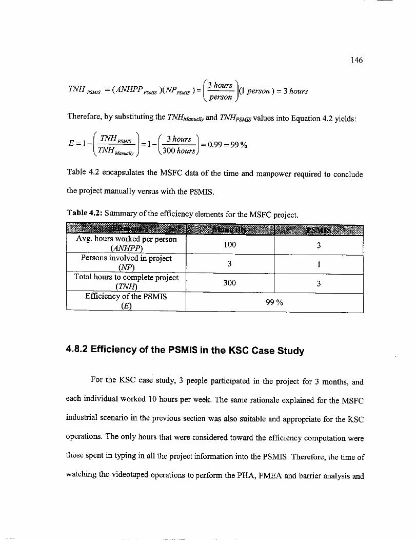
146
_I3_ hours )TNH PSM.,S= ( ANHPP esMIS)( NPpsM_S )-k person (1 person ) = 3 hours
Therefore, by substituting the TNHM.n,.,,,tty and TNHpsMIS values into Equation 4.2 yields:
E=I-( TNtteSM'S-/=1-( 3hours )
_,TNHMa,,,.lty ) k.3-_ _ours) = 0.99 = 99 %
Table 4.2 encapsulates the MSFC data of the time and manpower required to conclude
the project manually versus with the PSMIS.
Table 4.2: Summary of the efficiency elements for the MSFC project.
Avg. hours worked per person
(ANHPP)
Persons involved in project
(YP)
Total hours to complete project
(TN/-/)Efficiency of the PSMIS
(z)
100
3OO
3
99 %
4.8.2 Efficiency of the PSMIS in the KSC Case Study
For the KSC case study, 3 people participated in the project for 3 months, and
each individual worked 10 hours per week. The same rationale explained for the MSFC
industrial scenario in the previous section was also suitable and appropriate for the KSC
operations. The only hours that were considered toward the efficiency computation were
those spent in typing in all the project information into the PSMIS. Therefore, the time of
watching the videotaped operations to perform the PHA, FMEA and barrier analysis and

147
the time to manually record the dendriticoccurrencesin the samplingsheetswerenot
includedin the calculations.Consequently,thetime to becomefamiliar with theprocess
in orderto identify potentialhazardswasestimatedtobe2 weeksaswell.
Additionally, thesameassumptionfor theMSFC project,statingthat eachmonth
has4 weeks,wasmadein the KSC casestudy.Hence,theweeksencompassedin the 3-
months durationof the project are 12,but becauseof the 2 weeks spentin becoming
familiar with the process to recognizethe dendritics, the actual number of weeks
consideredin thecalculationsis 10.Thefull amountof hoursthat eachanalystworkedis
found by multiplying the actualnumberof weeksandthenumberof hoursthat heor she
worked in everyweek (10 hours);this equalsto a total of 100 hours.Since 3 persons
contributedto therealizationof theKSCproject,theANHPPM_nu_t yields the following:
(100 + 100 + 100) hours 1O0 hoursANHPP Man_Uy = =
3 persons person
By substituting this number into Equation 4.1, it results in:
=rlOO our 1TNH Manually= (ANHPPManu.IIy )(NPMan,,.Uy ) \ pe---rson---_" (3 persons ) = 300 hours
Likewise, the TNHpsMIS can be obtained. When the PSMIS was employed, the
KSC safety study was completed in 4 hours by 1 (one) person. Thus, the TNHpsMIs is
calculated in the following manner:
4 hours 4 hoursANHPP vs_rs - =
1 person person
I4h°ursl(lperson)=ahoursTNH PSMIS = (ANHPP PSMIS)( NPpsMIS ) = person
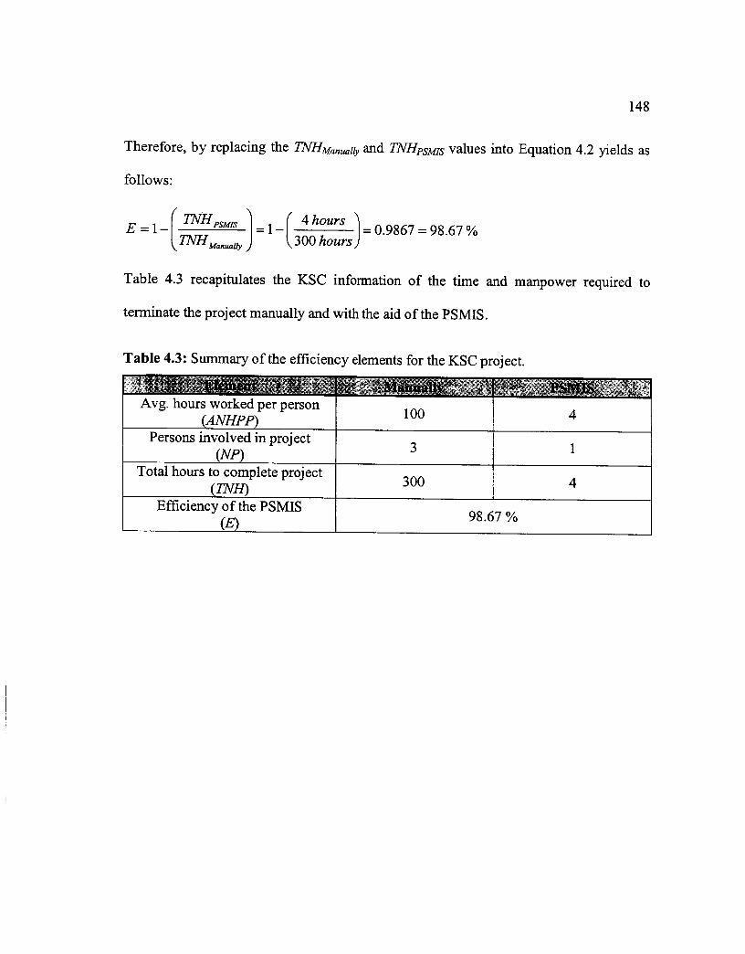
148
Therefore, by replacing the TNHManually and TNHpsMIS values into Equation 4.2 yields as
follows:
/ 1 ,,our Table 4.3 recapitulates the KSC information of the time and manpower required to
terminate the project manually and with the aid of the PSMIS.
Table 4.3: Summary of the efficiency elements for the KSC project.
Avg. hours worked per person
(ANHPP)
Persons involved in project
(NP)
Total hours to complete project
(TNH)Efficiency of the PSMIS
(E)
100
300
4
4
98.67 %
Chapter 5
5. CONCLUSIONS AND RECOMMENDATIONS
After implementing and evaluating the PSMIS, some deductions can be drawn as
well as some suggestions for future research. This chapter provides the conclusions and
recommendations pertaining to the research done and described in this project about the
development of a predictive safety management information system (PSMIS). This
management information system (MIS) comprises the theory of the Continuous Hazard
Tracking Failure Prediction Methodology (CHTFPM).
5.1 Introduction
The overview of this chapter is defined in this passage. Section 5.2 supplies a
summary of the work performed. In Section 5.3, the conclusions about the results of this
study are exposed while Section 5.4 discusses the potential implementation problems
with the PSMIS. To finish, Section 5.5 presents the recommendations for future studies
with the CHTFPM MIS/PSMIS.
5.2 Summary of Work Performed
The existing accident prevention models--like the ones revealed in Section
2.5.1--are either reactive or proactive in nature; however, not all of them are available in

150
a softwareapplication.The CHTFPMisapreventativesafetymodelthatis proactive,and
it hasbeenincorporatedinto a softwarepackage.By proactive,it is meantthat corrective
action is takenbeforethe fact, insteadof afterthefact, in orderto preventanaccidentor
system malfunction before occurring.To perform safety in a proactive manner,the
CHTFPM combinesthe principlesof safetysamplingand control charts.Therefore,the
CHTFPM MIS havethesetwo previousconceptsintegrated,sothat thesafetystatusof a
given systemor processcanbe known. Besidesthe PSMIS, therearesomepredictive
safety models that are proactiveand exist in the form of a softwaresystem(refer to
Section2.6.2.1and2.6.2.2).Nonetheless,thedisadvantageof thesecomputerprogramsis
that they areonly applicableto specificsitesor scenarios;whereastheCHTFPM MIS is
robust,meaningthat it is suitablefor manylocations,circumstancesandstudies.
In order to facilitate the applicationof thePSMIS and at the sametime provide
proof of the reliability and efficiency of the software,two previously validated case
studieswereselected.Thesetwopredictivesafetyprojectswerethefollowing:
1. Promotedcombustiontestingoperationsat the Material and CombustionResearch
Facility at MarshallSpaceFlight Center(MSFC).
2. Testing, preparation and hoisting operation of four high-pressuregas tanks
(HPGTs) at the Operationsand Check-Out Building at Kennedy SpaceCenter
(KSC).
The two studiesdepictedabovewere chosenfor the implementationof the CHTFPM
MIS. This signifies that all the informationencompassedin both projectswas input into
the PSMIS to verify if theresultsgivenby the softwarewerethe sameasthoseobtained

151
by hand. By doing so, the confidencein the results of the CHTFPM code could be
determined as well as the time necessary to complete the projects when the CHTFPM
MIS was used relative to when it was not used. This provided the implementation and
evaluation of the PSMIS.
5.3 Conclusions
The implementation and evaluation of the CHTFPM MIS on both case studies
revealed the following inferences:
• For the MSFC case study, the results presented by the PSMIS for each control
chart--c, weighted, EWMA (L=3.054, 2'=0.4 and L=2.814, 2,=0.1) and combined
Shewhart-EWMA chart--are exactly the same as the ones attained manually.
• For the MSFC case study, the Pareto diagram produced by the PSMIS is identical to
the one elaborated by the analyst.
• For the KSC case study, the results presented by the PSMIS for each control
chart----c and weighted chart--match those obtained by hand.
• For the KSC case study, the Pareto diagram fabricated by the PSMIS is equal to the
one constructed by the analyst.
• The PSMIS outcomes shown in Section 4.7 are evidence which undoubtedly
supports that the CHTFPM software system is reliable and accurate.
• In the MSFC project, 3 persons were required to finish off the research manually
resulting in 300 total number of hours (_HManually) spent.
152
• In the MSFC project, 1 person completed the study in 3 hours (TNHesmzs = 3) using
the PSMIS.
• In the MSFC project, there was a significant improvement in utilizing the CHTFPM
MIS versus doing the project manually, for the efficiency of the PSMIS was 99 %.
• In the KSC case study, it took 3 persons to conclude the research study for a total
number of hours (TNHManually) of 300.
• In the KSC case study, 1 person finalized the project in 4 hours (TNHPsMIs = 4).
• In the KSC case study, there was a significant improvement in utilizing the
CHTFPM MIS versus doing the research manually, for the efficiency of the PSMIS
was 98.67 %.
5.4 Potential Implementation Problems
The possible problems that could be faced when implementing or applying the
PSMIS are mainly related to collecting and, consequently, entering the data into the
CHTFPM MIS. This is true because the management of data, especially the calculations,
is handled by the computer program and not by the analyst. So, the program cannot give
incorrect results unless the user makes a mistake. For instance, when constructing a
Pareto diagram by manual means, the analyst can accidentally interchange the names of
the dendritics at the moment of assigning them to their respective frequencies (bars). This
would lead to wrong results and erroneous conclusions. Some of these potential problems
are described in the following list of points:
153
• The accuracyof the responsesgivenby the PSMISdependson the precision with
which the dendritic occurrences are entered. At the time of inputting such
information, the analyst can indicate by mistake that a certain dendritic occurred
when in reality it did not. This would give a variation in the plotted value of the
selected control chart or in the frequency of that dendritic in the Pareto diagram.
• When entering the number of dendritics observed into the PSMIS screens--which
correspond to a certain observation number--where the dendritic incidences are
typed in, the user can accidentally skip one or more observation numbers (screens).
• If an inspection screen was not filled out on purpose because no dendritics occurred
in that observation, the CHTFPM MIS will assume that such observation was not
conducted and will not be considered for any associated calculations, such as
sample size, control limits, plotted subgroup value, etc (review Section 3.8.2 to
avoid this kind of problem).
• The analyst can forget to conduct an observation to check for the presence of
dendritics in the system or can forget to input the dendritic occurrences into the
CHTFPM system. Therefore, such observation number will be left in blank and will
affect that particular subgroup size (refer to Section 3.8.2 to rectify this type of
problem).
• If an inspection number is skipped in the PSMIS due to any of the reasons cited in
this section, or for some other reason, it implies that not all the subgroups have the
same sample size. As a consequence, the CHTFPM MIS will try to graph a u chart
by default, at the time of specifying which type of control chart to view, since this is

154
the only attributechart that doesnotcarry therestrictionof equalsamplesize.The
computerprogram,however,will displayawarning/messagebeforeplotting the u
chart (read Section 3.8.2 to leam how to correct this problem).
5.5 Future Research Recommendations
The goal of this research has been to devise a predictive safety sot'cware to control
conditions leading to hazards fxom a proactive, instead of a reactive, standpoint. The
CHTFPM MIS can be used as a starting point for future research to enhance the
effectiveness of proactive safety projects. The recommendations for areas of future
research include the following:
• Add to the PSMIS a multivariate EWMA (MEWMA) which can demonstrate a
situation in which simultaneous monitoring and control of two or more related
quality characteristics (variables) is necessary.
• Incorporate into the CHTFPM code the capability to perform a discriminant
analysis to check the adequacy of the control charts and to generate an equation that
could be utilized for prediction of system safety.
• Test and implement the PSMIS beta version (first edition) in other NASA facilities
where the collection of data would be carried out in a real-time basis, hence in live
industrial scenarios. This would serve to further validate the PSMIS (based on user
input) and improve the usability of the CHTFPM MIS.

References
1. Bologna, Sandro and Hollnagel, Erik, 2002. Human-computer system dependability,
Computer Safety, Reliability and Security--Stuart Anderson, Sandro Bologna and
Massimo Felici, Eds.---(21 st International Conference, SAFECOMP), pp. 1-3,
Springer.
2. Borror, C. M.; Champ, C. W. and Rigdon, S. E., 1998. Poisson EWMA control
charts, Journal of Quality Technology, Vol. 30, No. 4, pp. 352-361.
3. BSI, 1991. British Standard Institution. Reliability of Systems, Equipments and
Components: Part 5 Guide to Failure Modes, Effects and Critically Analysis, BS
5760.
4. Chelbi, A. and Ait-Kadi, D., 1998. Inspection and predictive maintenance strategies,
International Journal of Computer-Integrated Manufacturing, Vol. 11, pp. 226-
231.
5. Cheng, Min-Yuan; Ko, Chien-Ho and Chang, Chih-Hung, 2002. Computer-aided
DSS for safety monitoring of geotechnical construction, Automation in
Construction, Vol. 11, pp. 375-290.
6. Cooper, J., 1998. Portraying information about sources of data in probabilistic
analyses, Proceedings of the 1998 ASME/JSME Joint Pressure Vessels and
Piping Conference. Vol. 378, pp. 26-30.
7. Dale, C. J. and Foster, S., i987. The development of techniques for safety and
reliability assessment: past, present and future, Achieving Safety and Reliability
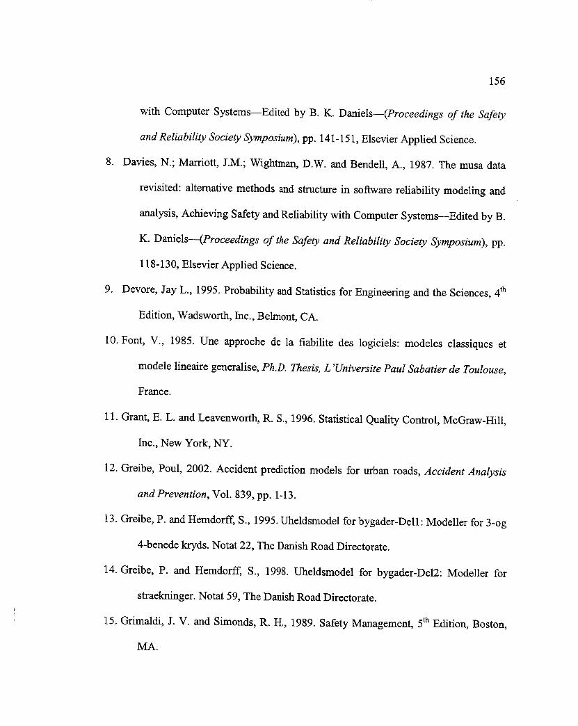
156
with ComputerSystems--Editedby B. K. Daniels--(Proceedingsof the Safety
and Reliability Society Symposium), pp. 141-151, Elsevier Applied Science.
8. Davies, N.; Marriott, J.M.; Wightman, D.W. and Bendell, A., 1987. The musa data
revisited: alternative methods and structure in software reliability modeling and
analysis, Achieving Safety and Reliability with Computer Systems--Edited by B.
K. Daniels---(Proceedings of the Safety and Reliability Society Symposium), pp.
118-130, Elsevier Applied Science.
9. Devore, Jay L., 1995. Probability and Statistics for Engineering and the Sciences, 4 th
Edition, Wadsworth, Inc., Belmont, CA.
10. Font, V., 1985. Une approche de la fiabilite des logiciels: modeles classiques et
modele lineaire generalise, Ph.D. Thesis, L 'Universite Paul Sabatier de Toulouse,
France.
11. Grant, E. L. and Leavenworth, R. S., 1996. Statistical Quality Control, McGraw-Hill,
Inc., New York, NY.
12. Greibe, Poul, 2002. Accident prediction models for urban roads, Accident Analysis
and Prevention, Vol. 839, pp. 1-13.
13. Greibe, P. and Hemdorff, S., 1995. Uheldsmodel for bygader-Dell: Modeller for 3-og
4-benede kryds. Notat 22, The Danish Road Directorate.
14. Greibe, P. and Hemdorff, S., 1998. Uheldsmodel for bygader-Del2: Modeller for
straekninger. Notat 59, The Danish Road Directorate.
15. Grimaldi, J. V. and Simonds, R. H., 1989. Safety Management, 5th Edition, Boston,
MA.

157
16.Guria, Jagadishand Mara, Kelly, 2000. Monitoring performanceof road safety
programmesin New Zealand,Accident Analysis and Prevention, Vol. 32, pp. 695-
702.
17. HSC, 1992. Health and Safety Commission. Management of Health and Safety at
Work Regulations, HSC Approved Code of Practice, ISBN 0-11-886330-4.
18. Hunter, J. S., 1986. The exponentially weighted moving average, Journal of Quality
Technology, Vol. 18, No. 4, pp. 203-210.
19. Johnson, W., 1995. Nuclear plant maintenance: NMAC's perspective, Proceedings of
the American Power Conference, Vol. 57, pp. 514-518.
20. Juran, J. M. and Gryna, F. M., Eds., 1988. Juran's Quality Control Handbook, 4 th
Edition, McGraw-Hill, Inc., New York, NY.
21. Ka_aiche, Mohamed; Laprie, Jean-Claude and Blanquart, Jean-Paul, 2002. A
fi:amework for dependability engineering of critical computing systems, Safety
Science, Vol. 40, pp. 731-752.
22. Kaplan, S., 1991. Risk Assessment and Risk Management - Basic Concepts and
Terminology, Hemisphere Publishing, New York, NY.
23. Kolarik, William J., 1999. Creating Quality: Process Design for Results, McGraw-
Hill Companies, Inc, New York, NY.
24. Koval, D. O., 1997. Human element factors affecting reliability and safety, Record of
Industrial and Commercial Power Systems Technical Conference, pp. 14-21.
25. Lee, Charles; Garnsworthy, Jon; Chudleigh, Morris and Bishop, Duncan, 1998. Issues
in managing a safety-critical system development project, Industrial Perspectives
158
of Safety-critical Systems--Editedby Felix Redmill and Tom Anderson-
(Proceedingsof the Sixth Safety-critical Systems Symposium), pp. 1-26, Springer.
26. Levinson, W. A. and Tumbelty, F., 1997. SPC Essentials and Productivity
Improvement: A Manufacturing Approach, ASQC Quality Press, Milwaukee, WI.
27. Lucas, J. M. and Saccucci, M. S., 1990. Exponentially weighted moving average
control schemes: properties and enhancements, Technometrics, Vol. 32, No. 1, pp.
1-29.
28. Mackie, R.I., 1998. An object-oriented approach to fully interactive finite element
software, Advances in Engineering Software, Vol. 29, No. 2, pp. 139-149.
29. Mackie, R.I., 2001. Implementation of sub-structuring within an object-oriented
framework, Advances in Engineering Software, Vol. 32, pp. 749-758.
30. Mangonon, Pat L., 1999. The Principles of Materials Selection for Engineering
Design, Prentice-Hall, New Jersey.
31. Marcombe, J. T., 1993. Behavior-based safety at Monsanto's Pensacola plant,
Chemical Engineer (London), No. 541, pp. 15-17.
32. Marshall, G., 1982. Safety Engineering, Brooks/Cole Engineering Division,
Monterey, CA.
33. Martin, James, 1987. Recommended Diagramming Standards for Analysts &
Programmers: A Basis for Automation, Prentice-Hall, Inc., Englewood Cliffs, NJ.
34. Meister, D., 1985. Behavioral Analysis and Measurement Methods, John Wiley and
Sons, New York, NY.

159
35.Montgomery, Douglas C., 1996. Introduction to Statistical Quality Control, 3rd
Edition, JohnWiley andSons,NewYork, NY.
36.Nagel, P.M. and Skrivan, J.A., 1981. Software reliability: repetitive run
experimentationand modeling,Boeing Computer Services Co. Report, BLS-
40366, NASA report No. CR-165836.
37. Ng, C. H. and Case, K. E., 1989. Development and evaluation of control charts using
exponentially weighted moving averages, Journal of Quality Technology, Vol. 21,
No. 4, pp. 242-250.
38. Norin, Hans and Isaksson-Hellman, Irene, 1995. Injury potential prediction of a
safety design feature: A theoretical method based on simulations and traffic
accident data, Safety Science, Vol. 19, pp. 45-56.
39. Norin, H.; Jemstr6m, C.; Koch, M.; Ryrberg, S. and Svensson, S-E., 1991. Avoiding
suboptimized occupant safety by multiple speed impact testing, 13 th ESV Conf.,
Paris, pp. 1-17, Paper No. 91-$9-O-89.
40. Olsen, D. A., 1993. CEO's Can Reform Workers' Compensation, The New York
Times, January 3, New York, NY.
41. Preyssl, C., 1995. Safety risk assessment and management - the ESA approach,
Reliability Engineering and System Safety, Vol. 49, pp. 303-309.
42. Quintana, R., Camet, M. and Deliwala, B., 2001. Application of a predictive safety
model in a combustion testing environment, Safety Science, Vol. 38, pp. 183-209.
43. Roland, H.E. and Moriarity, B., 1983. System Safety Engineering and Management,
John Wiley and Sons, New York, N'Y.
160
44.Ryan, T. P., 1989. StatisticalMethodsfor Quality Improvement,JohnWiley and
Sons,New York, NY.
45. Shell, R. L., Ed., 1986. Work Measurement:Principles and Practice, Industrial
EngineeringandManagementPress,Atlanta,GA.
46. Spalding, Ian, 1998. Principles of engineering safety management,Industrial
Perspectivesof Safety-critical Systems--Edited by Felix Redmill and Tom
Anderson--(Proeeedingsof the Sixth Safety-critical Systems Symposium), pp. 27-
43, Springer.
47. TNO Road-Vehicle Research Institute, 1990. MADYMO, Databases, Version 4.3,
The Netherlands.
48. TNO Road-Vehicle Research Institute, 1990. MADYMO, Users Manual 3D, Version
4.3, The Netherlands.
49. Veevers, A.; Petrova, E. and Marshall, A. C., 1987. Statistical methods for sotlware
reliability assessment, past, present and future, Achieving Safety and Reliability
with Computer Systems--Edited by B. K. Daniels--(Proceedings of the Safety
and Reliability Society Symposium), pp. 141-151, Elsevier Applied Science.
50. Vining, G. G., 1998. Statistical Methods for Engineers, Duxbury Press, New York,
NY.
51. Whitten, Jeffrey L.; Bentley, Lonnie D. and Barlow, Victor M., 1989. Systems
Analysis & Design Methods, 2 ndEdition, Richard D. Irwin, Inc., Boston, MA.
161
52. Wightman,D. W. andBendell,A., 1986.Proportionalhazardsmodelingof soRware
failure data, SoftwareReliability, State of the Art Report, 14:2, pp. 230-242,
Pergamon Infotech, Oxford.
53. Williams, B., 1978. A Sampler on Sampling, John Wiley and Sons, New York, NY.
54. Wilson, P. F.; Dell, L.D. and Anderson, G. F., 1993. Root Cause Analysis: A Tool for
Total Quality Management, ASQ Quality Press, Milwaukee, WI.
55. Wise, S. A. and Fair, D. C., 1998. Innovative Control Charting, ASQC Quality Press,
Chicago, IL.
56. Wrench, Constance P., 1990. Data Management for Occupational Health and Safety:
A User's Guide to Integrating Software, Van Nostrand Reinhold, New York, NY.
57. Zissler, J., 1996. Predictive hydraulic maintenance, Occupational Health and Safety,
Vol. 65, pp. 62-65.
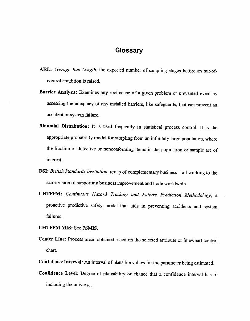
Glossary
ARL: Average Run Length, the expected number of sampling stages before an out-of-
control condition is raised.
Barrier Analysis: Examines arty root cause of a given problem or unwanted event by
assessing the adequacy of any installed barriers, like safeguards, that can prevent an
accident or system failure.
Binomial Distribution: It is used frequently in statistical process control. It is the
appropriate probability model for sampling from an infinitely large population, where
the fraction of defective or nonconforming items in the population or sample are of
interest.
BSI: British Standards Institution, group of complementary business--all working to the
same vision of supporting business improvement and trade worldwide.
CHTFPM: Continuous Hazard Tracking and Failure Prediction Methodology, a
proactive predictive safety model that aids in preventing accidents and system
failures.
CHTFPM M-IS: See PSMIS.
Center Line: Process mean obtained based on the selected attribute or Shewhart control
chart.
Confidence Interval: An interval of plausible values for the parameter being estimated.
Confidence Level: Degree of plausibility or chance that a confidence interval has of
including the universe.
163
Control Chart: A simple graphical device for knowing, at a given instance of time,
whether or not a process is under control.
Demerit Scheme: Method of assigning demerits or weights to dendritics or problems
according to their severity.
Dendritics: Building blocks of hazards or conditions in a given system that are becoming
hazardous.
DSS: Decision Support System, a safety computer system designed to assist construction
engineers in monitoring and controlling the excavation conditions that could become
hazardous in construction sites.
FMEA: Failure Mode and Effect Analysis, is a bottom-up hazard analysis procedure of
identifying the failure modes of a system and determining the effects on the next
higher level.
Frequency: The tally or count of only the number of observations associated with each
object or item (dendritic, problem, individual, etc.)
Hazard: The potential for an activity, condition, or circumstance to produce harmful
effects.
Hazard Analysis: The process of identifying, anticipating and controlling hazards.
I-ISE: Health and Safety Executive, responsible for the regulation of almost all the risks
to health and safety arising from work activity in Great Britain.
LCL: Lower Control Limit, delineates the bottom safety boundary in a control chart for a
given system or process.

164
MADYMO: Mathematicalsimulationmodelsthatcanpredicttypeof injuriesin acertain
car accident configuration before the system (human) is exposed to harmful
circumstances.
Mean: The sum of valuesin a distributiondividedby the numberof values.It is oneof
themostcommonmeasuresof centraltendency.
MIS: Management Information System, computer application that is capable of
organizing, storing and retrieving information.
Normal Distribution: A bell shaped distribution which describes most of the naturally
occurring phenomena. A normal distribution is identified by the mean and standard
deviation.
OSItA: Occupational Safety and Health Administration, an organization within the
Department of Labor, with a mission to ensure that every employer provides safe and
healthful conditions to every working man and woman.
Parameter: A constant or coefficient of a universe that describes some characteristic of
its distribution.
Pareto Analysis: A technique for prioritizing types or sources of problems by separating
the major causes from the minor causes of a problem (dendritics). This allows for a
focus on problems that offer the greatest potential for process improvement by using
a Pareto chart of diagram.
Pareto Chart: Also known as Pareto diagram. It is a bar graph that represents the
frequencies of dendritics or problems.
165
Percent Error: Desired or specified a, this is the probability of data falling outside the
confidence level.
PHA: Preliminary Hazard Analysis, is a system safety analysis tool which identifies
critical safety areas, evaluates hazards, and identifies the safety design criteria to be
used in order to eliminate or reduce the risk.
Poisson Distribution: It is a typical application in statistical process control. It is a
model of the number of defects or nonconformities that occur in a unit or product. In
fact, any random phenomenon that occurs on a per unit (or per unit area, per unit
volume, per unit time, etc.) basis is often well approximated by the Poisson
distribution.
Population: See universe.
Probability: The proportion of an object or thing (dendritic, problem, etc.) in a given
class, group, collection or set or data.
PSMIS: Predictive Safety Management Information System, software package that
incorporates the theory of the CHTFPM and performs data handling, data
manipulation as well as calculations automatically.
Random: An intuitive concept referring to a condition that happens unpredictably and
without any apparent pattern or reason. Equal chance of probability of occurrence for
each member of a group.
Risk: A measure of both the likelihood and consequences of all hazards of an activity or
condition. It is the chance of injury, damage or loss.
166
Risk Analysis: Method of applying qualitative and quantitative techniques to measure
potential risk in terms of frequency and severity rate.
Safety: Is the state of being relatively free from harm, danger, injury or damage.
Safety Engineering: Is the application of engineering principles to the recognition and
control or hazards.
Safety Sampling: A proactive approach for accident and system failure prevention by
monitoring the occurrence of dendritics in order to determine if a system is operating
within the specified control limits.
Sample: Portion or subset of objects or items from a larger set called universe.
Sampling: The activity or picking a sample from a universe to draw inferences about the
universe.
Significance: Means that a result differs from or exceeds some hypothetical value by
more than it can reasonably be attributed to the chance errors of sampling.
Standard Deviation: The measure of the dispersion of the observed values about their
mean.
UCL: Upper Control Limit, delineates the top safety boundary in a control chart for a
given system or process.
Universe: The set of all individuals or objects of a particular type.

APPENDIX A
Preliminary Hazard Analysis for the MSFC Project
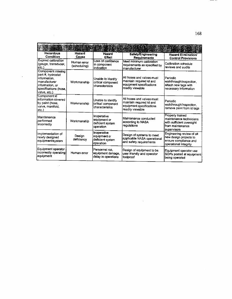
168
HazardousCondition
Expired calibration(gauge, transducer,etc.)Component missingpart #, hydrostatinformation,manufacturerinformation, orspecifications (hose,valve, etc.)Component idinformation coveredby paint (hose,valve, manifold,etc.)
Maintenanceperformedincorrectly
;Implementation ofnewly designedequipment/system
Equipment operatorincorrectly operatingequipment
Hazard Hazard Safety/EngineeringCause Effect Requirements
Human error Loss of confidence Meet minimum calibraUon;in component requirements as specified by
(scheduling) indication manufacturer
Workmanship
Workmanship
Workmanship
Designdeficiency
Human error
Unable to identifycritical componentcharacteristics
Unable to identifycritical componentcharacteristics
Inoperativeequipment ordeficient systemoperation
Inoperativeequipment ordeficient systemoperation
Personnel risk,equipment damage,delay in operations
All hoses and valves mustmaintain required id andequipment specificationsreadily viewable
All hoses and valves mustmaintain required id andequipment specificationsreadily viewable
Maintenance conducted
according to NASAregulations
Design of systems to meetapplicable NASA operationaland safety requirements
Design of equipment to beuser friendly and operatorfoolproof
Hazard Elimination/Control Provisions
Calibration schedulereviews and audits
Periodicwalkthrough/inspection,attach new tags withnecessary information
Periodic
walkthrough/inspection,remove paint from id tags
Properly trainedmaintenance technicianswith sufficient oversightfrom maintenance
supervisors
Equipment operator useSOPs posted at equipmentbeing operated
Engineering review of allnew design projects toensure compliance andoperational integrity
APPENDIX B
Failure Mode and Effect Analysis for the MSFC Project

170
NIA
NIA
NIA
CalibrationTechnician
A. Fails to calibrate equipmentPerforms IbY due datecalibration of 13-..Schedulingassigned D. Inspection of calibrationequipment records, visible discrepancy in(gauges, equipment, etc ..transducers, E. Calibrateetc) F. Varying
G. Yet to be determined
LubricationTechnician
A. Fails to lubricateB. Scheduling, negligence /
Lubricates all oversightrotors, rings and D. Inspection of maintenanceother parts records, visible discrepancy inneeding equipment, etc..lubrication E. Lubricate
F. VaryingG. Yet to be determined
Post-TestSystem
Operator
Equipmentshutdowninspection,clean-up andsimilar post-operationaltasks
A. Fails to properly shutdown,inspect, clean-up equipmentand/or its componentsB. Human error / oversightD. Operational problem / failuresafety infringement recognition /discrepancyE. Increase adherence to post-test procedures guidelinesand/or checklists, enlarged focuson safety standards, etc.
F. VaryingG. Yet to be determined
[] Loss ofconfidence in
equipmentindication /operation Possible effects[] Possible failure include minor tocause in function / severe personneluse / operation of risks, systemequipment or component failure,system ,stem failuret3 Possible factor
=nequipmentdowntime and / orlife expectancy
El Possible failurecause in function /use / operation
[] Possible factor Possible effectsIn equipment include minor todowntime and / or severe personnel
life expectancy risks, systemU Loss of component failure,confidence in system failure
equipmentindication /
operation
[] Possibility ofmultiple effects Possible effectsranging from include minor tominor to major severe personnelequipment failure risks, system/ hazard and / or component failure,component failure system failure/ hazard

171
/A
:/A
Sample Prepares, loads,Technician / unloads and / or
Handler handles testsamples
MaintenanceTechnician
ElectricalSystem
Components
Performscorrective and /or predictivemaintenance
Electricalconnections,components
A. Fails to propedy prepare,load, unload and / or handle testsamples as well as tabulatingsample informationB. Possible causes includehuman error / oversight,chemical impotency, mechanicalmalfunction of pads related toloading / unloading of samples,measurement of sampleproperties and so onD Notable abnormality ofsample or sample handling,
discrepancy in sample datasheets, improper sample
'situation in chamberE. Prepare sample again oracquire new sample, re-loadsample, improved adherence to}mcedural guidelines in sam }le
preparation, loading andhandlingF. VaryingG. Yet to be determined
A. Incorrectly performsmaintenanceB. WorkmanshipD. inspection of maintenancerecords, visible discrepancy inequipment, etc.E. Perform the maintenancetasks
F. VaryingG. Yet to be determined
A. Improper function / use /connection of electricalapparatus and electroniccomponentsB. VariousD. Visual or functionaldiscrepancy of equipment and /or its componentsE. Repair or replacement offaulty part / apparatusF. VaryingG. Yet to be determined
C] Possibility of Possible effectsmultiple effects include personnelranging from risks, system
minor to major component failure, 3equipment failure system failure, test
lazard and / or biasing and saml)lecomponent failure corruption/ hazard
0 Loss ofconfidence in
equipmentindication /operation
0 Loss ofconfidence inequipmentindication /
[] Possible failurecause in function /use / operation ofequipment ors_s_s_stem[] Possible factorin equipmentdowntime and / or
life expectancy J
Possible effectsinclude minor tosevere personnelrisks, systemcomponent failuresystem failure
Possible effectsinclude minor to
severe personnelrisks, systemcomponent failuresystem failure
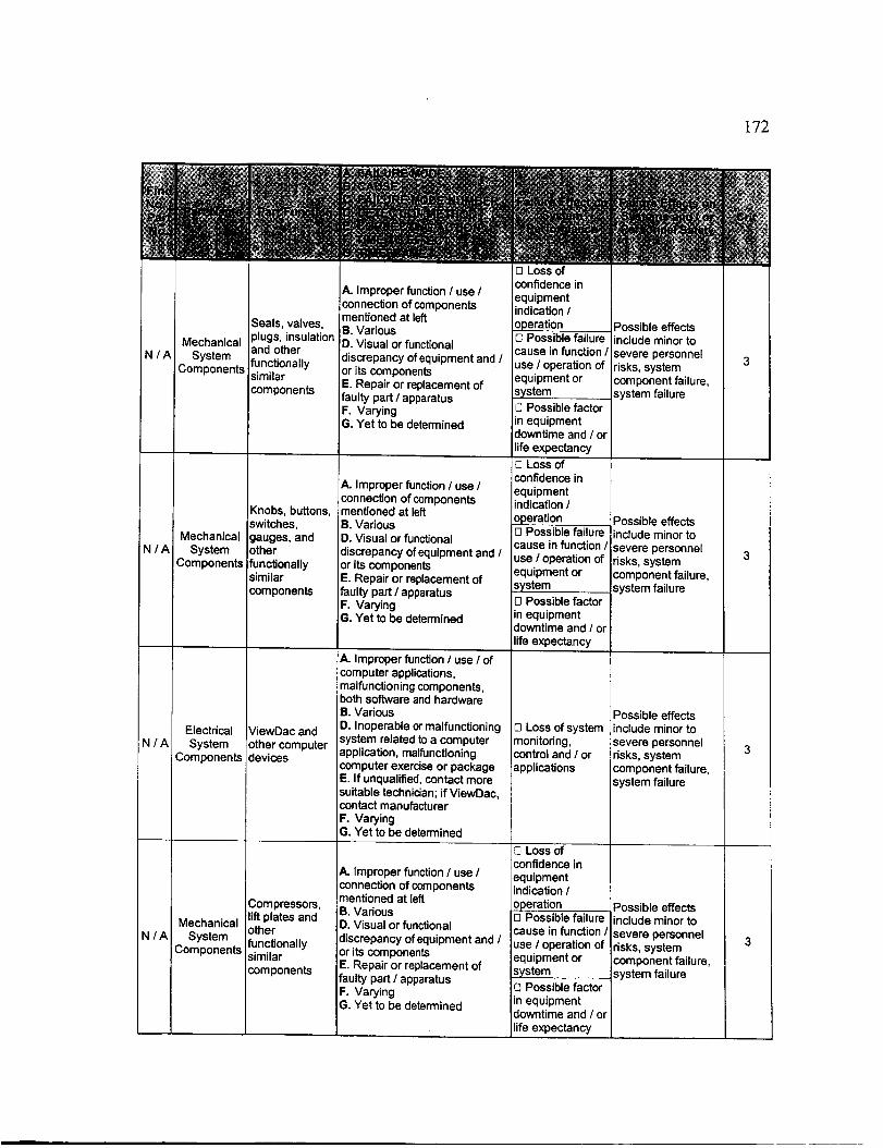
172
_I/A
Seals, valves,
Mechanical plugs, insulationand other
System functionallyComponents similar
components
Knobs, buttons,switches,
Mechanical gauges, and
q / A System other! Components functionally
similarcomponents
H/AElectrical ViewDac and
System other computerComponents devices
NIA
Compressors,lift plates and
Mechanical otherSystem funcUonally
Components similar
components
A. Improper function / use /connection of componentsmentioned at leftB. VariousD. Visual or functional
discrepancy of equipment and /or its componentsE. Repair or replacement offaulty part / apparatusF. VaryingG. Yet to be determined
A. Improper function / use /connection of componentsmentioned at leftB. VariousD. Visual or functionaldiscrepancy of equipment and /or its componentsE. Repair or replacement offaulty part / apparatusF. VaryingG. Yet to be determined
A. Improper function / use / ofcomputer applications,malfunctioning components,both software and hardwareB. VariousD. Inoperable or malfunctioningsystem related to a computerapplication, malfunctioningcomputer exercise or packageE. If unqualified, contact moresuitable technician; if ViewDaccontact manufacturerF. VaryingG. Yet to be determined
A. Improper function / use /connection of componentsmentioned at leftB. VariousD. Visual or functional
discrepancy of equipment and /or its componentsE. Repair or replacement offaulty part / apparatusF. VaryingG. Yet to be determined
[3 Loss ofconfidence inequipmentindication /
operation Possible effects[] Possible failure include minor to
cause in function / severe personneluse / operation of risks, systemequipment or component failure,system system failure[] Possible factorm equipmentdowntime and / orlife expectancy
{3 Loss ofconfidence inequipmentindication /
operation _ Possible effects[] Possible failure include minor to
cause in function / severe personneluse / operation of risks, systemequipment or component failure,system _ system failure[] Possible factor=nequipmentdowntime and / orlife expectancy
Possible effects[] Loss of system include minor tomonitoring, severe personnelcontrol and / or risks, systemapplications component failure
system failure
[] Loss ofconfidence inequipmentindication /operation Possible effects[] Possible failure include minor tocause in function / severe personneluse ! operation of risks, systemequipment or component failure.system system failure[] Possible factorm equipmentdowntime and / orlife expectancy

APPENDIX C
Barrier Analysis for the MSFC Project
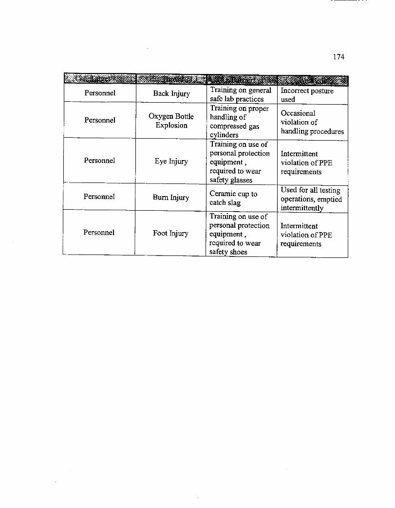
174
Personnel
Personnel
Personnel
Personnel
Personnel
Back Injury
Oxygen Bottle
Explosion
Eye Injury
Burn Injury
Foot Injury
Training on general
safe lab practices
Training on proper
handling of
compressed gas
cylinders
Training on use of
personal protection
equipment,
required to wear
safety glasses
Ceramic cup to
catch slag
Training on use of
personal protection
equipment,
required to wear
safety shoes
Incorrect postureused
Occasional
violation of
handling procedures
Intermittent
violation of PPE
requirements
Used for all testing
operations, emptied
intermittently
Intermittent
violation of PPE
requirements
APPENDIX D
c Control Chart Data for the MSFC Project

176
0 51 3
1 52 1
2 53 1
54
55
6 3 56
7 4 57
8 4 58
9 3 59
10 60
2
3
3
1
2
11 2
12 1
61 3
62 3
63 213 3
14 2 64 2
15 2 65 2
16 0
17 0
18 0
19 1
20 1
21
22
23
66 7
67 3
68 3
69 3
70 1
71
72
73
74
75
24
25
26 0 76
27 0 77
28 4 78
29 0 79
30 80
4
98 0
49 0 99 0
50 7 100 0
46 2
47 3
48 3
42 0 92
43 0 93
44 2 94
45 2 95
91
96
97
41 0
31 1 81 0
32 1 82 0
33 0 83 0
34 1 84 1
35 1 .85 1
36 1 86 2
37 1 87 2
38 0 88 2
39 0 89 4
40 1 90 3
APPENDIX E
Weighted Control Chart Data for the MSFC Project
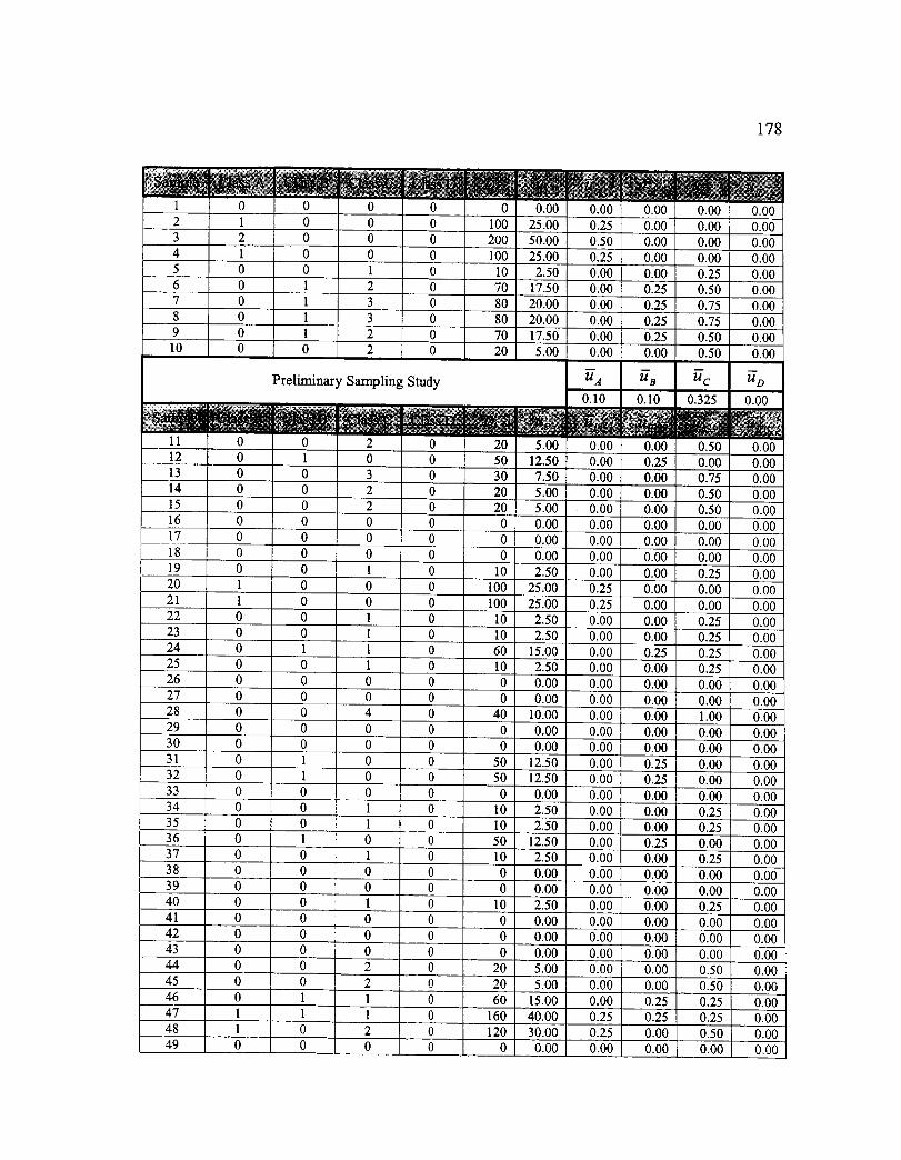
178
1 0
2 1 0 0 0
3 2 0 0 0
4 1 0 0 0
5 0 0 1 0
6 0 I 2 0
7 0 1 3 0
8 0 1 3 0
9 0 1 2 0
10 0
0 0.00100 25.00
200 50.00
100 25.00
10 2.50
70 17.50
80 20.00
80 20.00
70 17.50
20 5.00
Preliminary Sampling Study
11 0 0 2 0 20 5.00
12 0 1 0 0 50 12.50
13 0 0 3 0 30 7.50
14 0 0 2 0 20 5.00
15 0 0 2 0 20 5.00
0 0.00
0 0.00
0 0.00
10 2.50
100 25.00
100 25.00
10 2.50
10 2.50
60 15.00
10 2.50
0 0.00
0 0.00
40 10.00
0 0.00
0 0.00
50 12.50
50 12.50
0 0.00
I0 2.50
10 2.50
50 12.50
10 2.50
0 0.00
0 0.00
10 2.50
0 0.00
0 0.00
0 0.00
20 5.00
20 5.00
60 15.00
160 40.00
120 30.00
0 0.00
16 0 0 0 0
17 0 0 0 0
18 0 0 0 0
19 0 0 1 0
20 1 0 0 0
21 1 0 0 0
22 0 0 1 0
23 0 0 1 024
25
0 1 1 0
0 0 1 0
26 0 0 0 0
27 0 0 0 0
28 0 0 4 0
29 0 0 0 0
30 0 0 0 0
31 0 1 0 0
32 0 1 0 0
33 0 0 0 0
34 0 0 1 0
35 0 0 1 0
36 0 1 0 0
37 0 0 1 0
38 0 0 0 0
39 0 0 0 0
40 0 0 1 0
41 0 0 0 0
42 0 0 0 0
43 0 0 0 0
44
45
46
47
48
49
0 0 2 0
0 0 2 0
1 1 0
1 1 0
0 2 0
0 0 0
&oo o.oo o.oo o.o00.25 0.00 0.00 0.00
0.50 0.00 0.00 0.00
0.25 0.00 0.00 0.00
0.00 0.00 0.25 0.00
0.00 0.25 0.50 0.00
0.00 0.25 0.75 0.00
0.00 0.25 0.75 0.00
0.00 0.25 0.50 0.00
0.00 0.00 0.50 0.00
0.10 0.10 0.325 0.00
0.00 0.00 0.50 0.00
0.00 0.25 0.00 0.00
0.00 0.00 0.75 0.00
0.00 0.00 0.50 0.00
0.00 0.00 0.50 0.00
0.00 0.00 0.00 0.00
0.00 0.00 0.00 0.00
0.00 0.00 0.00 0.00
0.00 0.00 0.25 0.00
0.25 0.00 0.00 0.00
0.25 0.00 0.00 0.00
0.00 0.00 0.25 0.00
0.00 0.00 0.25 0.00
0.00 0.25 0.25 0.00
0.00 0.00 0.25 0.00
0.00 0.00 0.00 0.00
0.00 0.00 0.00 0.00
0.00 0.00 1.00 0.00
0.00 0.00 0.00 0.00
0.00 0.00 0.00 0.00
0.00 0.25 0.00 0.00
0.00 0.25 0.00 0.00
0.00 0.00 0.00 0.00
0.00 0.00 0.25 0.00
0.00 0.00 0.25 0.00
0.00 0.25 0.00 0.00
0.00 0.00 0.25 0.00
0.00 0.00 0.00 0.00
0.00 0.00 0.00 0.00
0.00 0.00 0.25 0.00
0.00 0.00 0.00 0.00
0.00 0.00 0.00 0.00
0.00 0.00 0.00 0.00
0.00 0.00 0.50 0.00
0.00 0.00 0.50 0.00
0.00 0.25 0.25 0.00
0.25 0.25 0.25 0.00
0.25 0.00 0.50 0.00
0.00 0.00 0.00 0.00
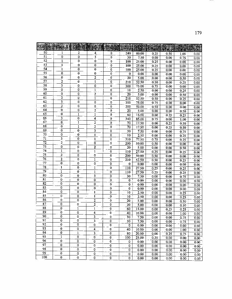
179
50 ............ i 2 4 0
3 051 0 052 1 0 053 1 0 054 1 055 0 0 0 056 0 0 2 057 2 1 0
58 3 059 0 060 0 061 2 062 3 063 2 0
0 01 02 01 00 00 0
64 0 0 2 065 0 166 3 067 0 168 0 169 0 070 0 071 3 072 2 073 0 074 1 075 2 076 2 077 0 078 1 079 1 08O 0 08l 0 082 0 083 0 084 0 085 0 086 0 087 0 088 0 189 0 090 0 091 0 0
1 04 02 02 03 01 01 00 02 01 00 01 00 01 01 03 00 00 00 01 01 02 02 01 04 03 03 0
92 0 0 0 093 0 094 0 1
4 03 0
95 1 0 0 096 0 0 0 097 0 098 0 0
"i °1°100 0 0
0 00 00 00 0
240 60.00 0.25 0.50 1.0030 7.50 0.00 0.00 0.75
100 25.00 0.25 0.00 0.00100 25.00 0.25 0.00 0.00100 25.00 0.25 0.00 0.00
0 0.00 0.00 0.00 0.0020 5.00 0.00 0.00 0.50
210 52.50 0.50 0.00 0.25
300 75.00 0.75 0.00 0.0010 2.50 0.00 0.00 0.2520 5.00 0.00 0.00 0.50
210 52.50 0.50 0.00 0.25300 75.00 0.75 0.00 0.00200 50.00 0.50 0.00 0.00
20 5.00 0.00 0.00 0.5060 15.00 0.00 0.25 0.25
340 85.00 0.75 0.00 1.0070 17.50 0.00 0.25 0.5070 17.50 0.00 0.25 0.5030 7.50 0.00 0.00 0.7510 2.50 0.00 0.00 0.25
310 77.50 0.75 0.00 0.25200 50.00 0.50 0.00 0.0020 5.00 0.00 0.00 0.50
110 27.50 0.25 0.00 0.25200 50.00 0.50 0.00 0.00210 52.50 0.50 0.00 0.25
0 0.00 0.00 0.00 0.00110 27.50 0.25 0.00 0.25110 27.50 0.25 0.00 0.2530 7.50 0.00 0.00 0.750 0.00 0.00 0.00 0.000 0.00 0.00 0.00 0.000 0.00 0.00 0.00 0.00
10 2.50 0.00 0.00 0.2510 2.50 0.00 0.00 0.2520 5.00 0.00 0.00 0.5020 5.00 0.00 0.00 0.5060 15.00 0.00 0.25 0.2540 10.00 0.00 0.00 1.0030 7.50 0.00 0.00 0.7530 7.50 0.00 0.00 0.750 0.00 0.00 0.00 0.00
40 10.00 0.00 0.00 1.0080 20.00 0.00 0.25 0.75
100 25.00 0.25 0.00 0.000 0.00 0.00 0.00 0.000 0.00 0.00 0.00 0.000 0.00 0.00 0.00 0.00
o ooooooI Oo. OI ooo0 0.00 0.00 . 0.00
0.000.000.000.000.000.000.000.00
0.000.000.000.000.000.000.000.000.000.000.000.000.000.000.000.000.000.000.000.000.000.000.000.000.000.000.000.000.000.000.000.000.000.000.000.000.000.000.000.000.000.000.00

APPENDIX F
EWMA Control Chart Data for the MSFC Project (,_= 0.4, L = 3.054)

181
1.26000 3.87027 0.32973
2 1 1.15600
3 2 1.49360
4 1 1.29616
5 1 1.17770
6 3 1.90662
10
11
12
13
14
15
16
17
18
19
20
21
22
2.74397
3.24638
3.14783
2.68870
2.41322
1.84793
2.30876
2.18526
2.11115
1.26669
0.76002
0.45601
0.85601
0.91361
0.94816
0.96890
4.16447 0.03553
4.26060 -0.06060= 0
4.29417 -0.09417 = 0
4.30613 -0.10613 = 0
4.31042 -0.11042 = 0
4.31197
4.31252
4.31272
4.31279
4.31282
4.31283
4.31283
4.31283
4.31283
4.31283
4.31283
4.31283
4.31283
4.31283
4.31283
4.31283
-0.11197 = 0
-0.11252 = 0-0.11272 = 0
-0.11279 = 0
-0.11282 = 0
-0.11283 = 0
-0.11283 = 0-0.11283 = 0
-0.11283 = 0
-0.11283 = 0
-0.11283 = 0
-0.11283 = 0
-0.11283 = 0
-0.11283 = 0
-0.11283 = 0
-0.11283 = 0
23 1 0.98134 4.31283 -0.11283 = 0
24 2 1.38880 4.31283 -0.11283 = 0
25 1 1.23328 4.31283 -0.11283 = 0
26 0 0.73997 4.31283 -0.11283 = 0
27 0 0.44398 4.31283 -0.11283 = 0
28 4 1.86639 4.31283 -0.11283 = 0
29 0 1.11983 4.31283 -0.11283 = 0
30 0 0.67190 4.31283 -0.11283 = 0
31 1 0.80314 4.31283 -0.11283 = 0
32 1 0.88188 4.31283 -0.11283 = 0
33 0 0.52913 4.31283 -0.11283 = 0
34 1 0.71748 4.31283 -0.11283 = 0
35 1 0.83049 4.31283 -0.11283 = 0
36 1 0.89829 4.31283 -0.11283 =0
37 1 0.93898 4.31283 -0.11283 = 0
38 0 0.56339 4.31283 -0.11283 = 0
39 0 0.33803 4.31283 -0.11283 = 0
40 1 0.60282 4.31283 -0.11283 = 0
41 0 0.36169 4.31283 -0.11283 = 042 0 0.21701 4.31283 -0.11283 = 0
43 0 0.13021 4.31283 -0.11283 = 0
44 2 0.87813 4.31283 -0.11283 = 0
45 2 1.32688 4.31283 -0.11283 = 0
1.5961346 4.31283 -0.11283 = 0
4.31283 -0.11283 = 0
4.31283 -0.11283 = 0
4.31283 -0.11283 = 0
47 3 2.15768
48 3 2.49461
49 0 1.49676
50 I 7 I 4.31283 -0.11283 = 0

182
51
52
53
54
55
56
57
58
59
6O
61
62
63
64
65
66
67
68
3 3.41883
2.45130
1.87078
1.52247
0.91348
1.34809
2.00885
2.40531
1.84319
1.90591
2.34355
2.60613
2,36368
2.21821
2.13092
4.07855
3.64713
3.38828
4.31283
4.31283
4.31283
4.31283
4.31283
4.31283
4.31283
4.31283
4.31283
4.31283
4.31283
4.31283
4,31283
4.31283
4.31283
4.31283
4.31283
4.31283
-0.11283 = 0
-0.11283 = 0
-0.11283 = 0
-0.11283 = 0
-0.11283 = 0
-0.11283 = 0
-0.11283 = 0
-0.11283 = 0
-0.11283 = 0
-0.11283 = 0
-0.11283 =0
-0.11283 = 0
-0.11283 = 0
-0.11283 = 0
-0.11283 = 0
-0.11283 = 0
-0.11283 = 0
-0.11283 = 0
69 3 3.23297 4.31283 -0.11283 = 0
70 1 2.33978 4.31283 -0.11283 = 0
71 4 3.00387 4.31283 -0.11283 = 0
72 2 2.60232 4.31283 -0.11283 = 0
73 2 2.36139 4.31283 -0.11283 = 0
74 2 2.21684 4.31283 -0.11283 = 0
75 2 2.13010 4.31283 -0.11283 = 0
76 3 2.47806 4.31283 -0.11283 = 0
77 0 1.48684 4.31283 -0.11283 = 0
78 2 1.69210 4.31283 -0.11283 = 0
79
80 3
81 0
82 0
83 0
84 1
85 1
86 2
87 2
88
89
9O
91
92
4.312831,81526 -0,11283 = 0
2.28916 4.31283 -0.11283 = 0
1.37349 4.31283 -0.11283 = 0
0.82410 4.31283 -0.11283 = 0
0.49446 4.31283 -0.11283 = 0
0.69667 4.31283 -0.11283 = 0
0.81800 4.31283 -0.11283 = 0
1.29080 4.31283 -0.11283 = 0
1.57448 4.31283 -0.11283 = 0
4.312831.74469
4.31283
4.31283
4.31283
4.31283
4.31283
4.31283
4.31283
4.31283
4.31283
2.64681
4.31283
2.78809
2.87285
1.72371
2.63423
3.18054
2,30832
1.38499
93
94
0.83100
95
96
97
98
-0.11283 = 0
I 0 0.17950
-0,11283 = 0
-0.11283 = 0
-0.11283 = 0
-0.11283 = 0
-0.11283 = 0
-0.11283 = 0
-0.11283 = 0
-0.11283 = 0
-0.11283 = 0
0 0.49860 4.31283 -0.11283 = 0
99 0 0.29916 4.31283 °0.11283 = 0
100 -0.11283 = 0

APPENDIX G
EWMA Control Chart Data for the MSFC Project (_.= 0.1, L = 2.814)

184
1 0 1.89000 2.50779
1 1.80100 2.64862 1.55138
2 1.82090 2.74038 1.45962
4 1 1.73881 2.80602
5 1 1.66493 2.85501
6 3 1.79844 2.89248
10
11
12
13
14
15
2.01859
2.21673
2.29506
2.26555
2.23900
2.11510
2.20359
2.18323
2.16491
1.94842
1.75357
16
17
18 0 1.57822
19 1 1.67822
20 1 1.6104021 1.54936
1.49442
1.44498
22
23
1.17485
24 2 1.50048
25 1 1.45043
26 0 1.30539
27 028 1.45737
1.14618
29 0 1.31163
30 0 1.18047
31 1 1.16242
32 1
1.37238
33 0 1.03156
34 1 1.02840
35 1 1.02556
36 1 1.02301
37 1 1.02071
38 0 0.91864
39 0 0.82677
40 1 0.84409
41 0 0.75969
42 0 0.68372
43 0 0.61535
44 2 0.75381
45 2 0.87843
46 2 0.99059
47 3 1.19153
48 3
2.92158
2.94441
2.96247
2.97682
2.98827
2.99744
3.00480
3.01072
3.01548
3.01933
3.02243
1.39398
1.34499
1.30752
1.27842
1.25559
1.23753
1.22318
1.21173
1.20256
1.19520
1.18928
1.18452
1.18067
1.17757
3.02493 1.17507
3.02695 1.17305
3.02859 1.17141
3.02991
3.030981.17009
1.16902
3.03185 1.16815
3.03255 1.16745
3.03311 1.16689
3.03357 1.16643
3.03395
3.03425
3.03449
49 0 1.23514
50 [ 7 1.81162
1.16605
1.16575
1.16551
3.03469 1.16531
3.03485 1.16515
3.03498
3.03508
1.16502
1.16492
3.03517 1.16483
3.03524 1.16476
3.03529 1.16471
3.03534 1.16466
3.03537 1.16463
3.03540 1.16460
3.03543 1.16457
3.03545 1.16455
3.03546 1.16454
3.03547 1.16453
3.03548 1.16452
3.03549 1.16451
3.03550 1.16450
3.03550 1.16450
3.03551
3.03551
1.16449
1.16449
3.03552 1.16448

185
51
52
53
54
55
56
57
58
59
60
61
62
63
3 1.93046 3.03552 1.16448
1 1.83742
1 1.75367
1 1.67831
0 1.51048
2 1.55943
3 1.70349
3 1.83314
I 1.74982
2 1.77484
3 1.89736
3 2.00762
2 2.00686
64 2 2.00617
65 2 2.00556
66 7 2.50500
67 3
68
69
70
71
72 2
73 2
74 2
75 2
76 3
77 0
78 2
79 2
80 3
81 0
82 0
83 0
84 1
85 1
86 2
87
88
89
90 3
91 3
92 0
93 4
94 495 1
96 0
97 0
98 0
99
100
2.55450
2.59905
2.63915
2.47523
2.62771
3.03552 1.16448
3.03552 1.16448
3.03552 1.16448
3.03552 1.16448
3.03552 1.16448
3.03553 1.16447
3.03553 1.16447
3.03553 1.16447
3.03553 1.16447
3.03553 1.16447
3.03553 1.16447
3.03553 1.16447
3.03553 1.16447
3.03553 1.16447
3.03553 1.16447
3.03553
3.03553
3.03553
1.16447
1.16447
1.16447
3.03553 1.16447
3.03553 1.16447
3.035532.56494 1.16447
2.50844 3.03553 1.16447
2.45760 3.03553 1.16447
3.035532.41184 1.164472.47066
2.22359
2.20123
2.18111
2.26300
2.03670
3.03553 1.16447
3.03553 1.16447
3.03553 1.16447
3.03553 1.16447
3.03553 1.164473.03553 1.16447
1.83303 3.03553 1.16447
1.64972 3.03553 1.16447
1.58475 3.03553 1.16447
1.52628 3.03553
1.57365
1.61628
1.65466
1.88919
2.00027
3.03553
3.03553
3.03553
3.03553
3.03553
3.03553
3.03553
3.03553
3.03553
3.03553
3.03553
3.03553
3.03553
3.03553
3.03553
2.10024
1.89022
2.10120
2.29108
2.16197
1.94577
1.75120
1.57608
1.41847
1.27662
1.16447
1.16447
1.16447
1.16447
1.16447
1.16447
1.16447
1.16447
1.16447
1.16447
1.16447
1.16447
1.16447
1.16447
1.16447
1.16447
APPENDIX H
Preliminary Hazard Analysis for the KSC Project

187
HazardousConditions
1. Non-hazard proofelectrical equipment
HazardCause
Hazard Effect
2. Hose rupture ofGSE leak.
3. AdiabaticCompression/Overt_mp
4. AcceleratedParticlevelocity/cleanliness
HumanError(Failure tofollow SOP)
Manufacturerdefect/hoselife
HumaneErrorFailure to
FollowDMSRDRequirements)
DesignDeficiency
Fire/Explosionresulting in injuryor death to)ersonal andloss of or
:lamage to flighthardware,3round SupportEquipment'_GSE),and:acility..ire/Explosion"esultingin injuryor death to3ersonal and_ossof or_lamage toflighthardware, GSE,and facility.
Fire/Explosionresulting in injuryor death to)ersonal andloss of ordamage to flighthardware, GSE,and facility.
Fire/Explosion-esulting in injuryor death topersonal andloss of ordamage to flighthardware, GSE,and facility.
Safety/Engineering
Requirements
Lock out and tag outall non-hazard proof_on-electrical,=quipment
Meet minimumcalibrationrequirements asspecified by themanufacturer.
Meet OMRSDrequirements define:he)ressurization/depressurization rates
PRUA cleaned tolevel 100A per KSC-SPEC-C-123.
Hazard EliminationControl Provisions
High Pressure Gas Tankstest work authorization)rocedures (WAP)contain steps requiring awalk down to verify thatall electrical equipmenthas been locked out andtagged.
Valid proof test andzalibration certificationshall be verified prior to"lazard operations. WADsshall contain steps thatverify that the proof testand calibrations arecurrent.Limit)ressurization/depressunzation at 50 psi/sec. Theaddition of an orificerestricting the flow rate ofthe Pressure RegulatingJnit Assembly (PRUA).Vlonitor and control tankLemperatures during fill_perations keeping temp._)elow 115 F. Incorporatemonitoring requirementsinto WAD.Addition of three 10-micron filters one in theinlet side of the PRUA,one is internal to thePRUA and one connectecto the HPGTs inlet supply/alve. Samples will be:aken to verify oxygenzleanliness prior to andafter HPGTs servicing.
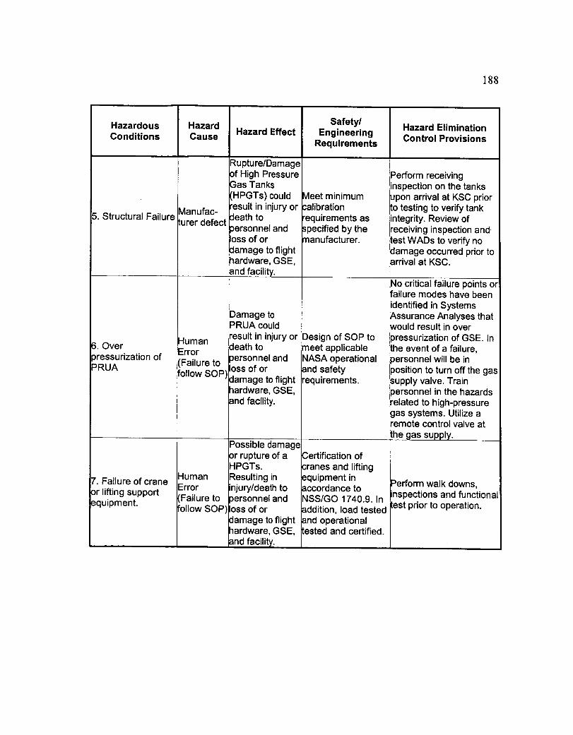
188
HazardousConditions Hazard Effect
5. Structural Failure
HazardCause
Manufac-turer defect,
5. Over HumanError)ressurization of
PRUA (Failure tofollow SOP)
Rupture/DamageDf High PressureGas TanksIHPGTs) could"esult in injury or:leath to3ersonnel andoss of orJamage to flight_ardware, GSE,and facility.
Damage to=RUA could"esult in injury or"leathto)ersonnel andloss of ordamage to flight
Safety/Engineering
Requirements
Meet minimumcalibrationrequirements asspecified by themanufacturer.
Design of SOP tomeet applicableNASA operationaland safetyrequirements.
Hazard EliminationControl Provisions
Perform receivingknspection on the tanksupon arrival at KSC priorto testing to verify tankintegrity. Review ofreceiving inspection andtest WADs to verify nodamage occurred prior toarrival at KSC.
No critical failure points or,failure modes have beenidentified in SystemsAssurance Analyses thatwould result in over)ressurization of GSE. Inthe event of a failure,)ersonnel will be in)osition to turn off the gassupply valve. Train
hardware, GSE,and facility.
Possible damage
)ersonnel in the hazardsrelated to high-pressuregas systems. Utilize aremote control valve atthe gas supply.
7. Failure of craneDr lifting support_quipment.
HumanErrorFailure toFollow SOP)
or rupture of aHPGTs.Resulting ininjury/death to_ersonnel andloss of ordamage to flighthardware, GSE,and facility.
Certification ofcranes and liftingequipment inaccordance toNSS/GO 1740.9. Inaddition, load testedand operationaltested and certified.
Perform walk downs,inspections and functionaltest prior to operation.

189
HazardousConditions
3. Impact with otherstructures.
HazardCause
HumanErrorFailure to;ollow SOP)
Hazard Effect
Possible damage3r rupture of aHPGT. Resultingin injury/death to3ersonnel andoss of or:lamage toflight3ardware, GSE,and facility.
Safety/Engineering
Requirements
If crane is at adistant greater than10 inches from astructure operationspeed has to be lessthan 2 in./min.Within 10-in. operateless than 1 in./min.
Hazard EliminationControl Provisions
Operators will posses avalid operator's license,which is verified in theWAD. Perform a pre-testbriefing shall be held priorto lifting operations and)ersonnel will be advisedof their specific task and:he hazards involved. Acontrolled area shall be_stablished for all lifting)perations and cleared ofall nonessential)ersonnel.
APPENDIX I
Failure Mode and Effect Analysis for the KSC Project

191
Tubing /Transport
Oxygen fromPRUA to HPGT
Non-hazard
proof electricalequipment / Nofunction
PRUA /
RegulatePressure
Communications
5uring hoisting
operations
Ignition
Electrical
arcing
Leaks/Fke
Improperoperations,confusion
duringanomalies,
exacerbatingemergencies
Fire/Explosionresulting in injuryor death to
personal and loss
of or damage toflight hardware,
Ground SupportEquipment (GSE),
and facility.
Fire/Explosion
resulting in injuryor death to
personal and lossof or damage to
flight hardware,Ground Support
Equipment (GSE),and facility.
Resulting in injuryor death to
personal and loss
of or damage toflight hardware,
Ground Support
Equipment (GSE),and facility.
Accident resulting11injury to9ersonal and loss
_f or damage to
flight hardware,3round Support
Equipment (GSE).
Striking a valve
body justdownstream of thecontrol element of
the valve can cause
Particulate Impactignition caused by
the exposure of un-oxidized metalsurfaces.
Short circuit and arc
through its sheath t_
the oxygen gas.Human Error
(Failure to followSOP).
Orifices and
regulators preclude
flow rates. Age ofEquipment
Human Error
(Failure to followSOP)
Five 10 Micronfilters remove
_articulates.
Lock out and tagout all non-
hazard proofnon-electrical
equipment.
Tested with
High-pressure
oxygen.Designed andcertified SSP500004. The
GOX supplysource is
external to the
)uilding and:apable ofisolation with a
:emote shut-offvalve.
_ystem layoutallows directcerbal and visual:ommunications.
All operators are
Iogether, nonelocated
remotely.
!iwi.mmunicati°ns
th other O &
11beablished.
Continue to use
five 10 Micronfilters remove
)articulates.
High PressureGas Tanks test
workauthorization3rocedures
_,WAD) contain
_teps requiringwalk down to
verify that all:lectrical
,_quipment has_een locked out
and tagged.Use a portable32-monitor
_ystem to detect
oxygen levels.
None
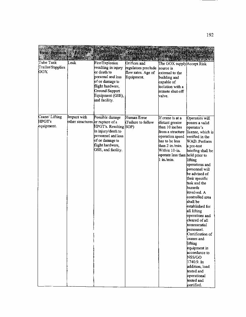
192
Fube Tank
trailer/SuppliesGOX
Crane/LiftingHPGT's
equipment.
Leak
Impact with3ther slructures.
Fire/Explosion
resulting in injuryor death to
personal and lossof or damage to
flight hardware,
Ground SupportEquipment (GSE),
and facility.
Possible damage
or rupture of aHPGT's. Resultingin injury/death to
personnel and lossof or damage to
flight hardware,
GSE, and facility.
Orifices and
regulators preclude
flow rates. Age ofEquipment.
Human ErrorTailure to follow
;,OP)
The GOX supplysource isexternal to the
building and
capable ofisolation with aremote shut-off
valve.
If crane is at a
t greater5aan 10 inches_rom a structure
3peration speedaas to be less
_han 2 in./min.Within 10-in.
operate less thanin./min.
Accept Risk
Operators will
posses a validoperator'slicense, which isverified in theWAD. Perform
a pre-testbriefing shall beheld prior to
lifting
operations andpersonnel willbe advised of
heir specificIask and theaazards
revolved. Azontrolled area
_hall be
established for
all lifting
operations andcleared of allnonessential
personnel.Certification ofcranes and
Lifting_quipment inaccordance to
NSS/GO1740.9. In
addition, load
sted andperational
sted andertified.
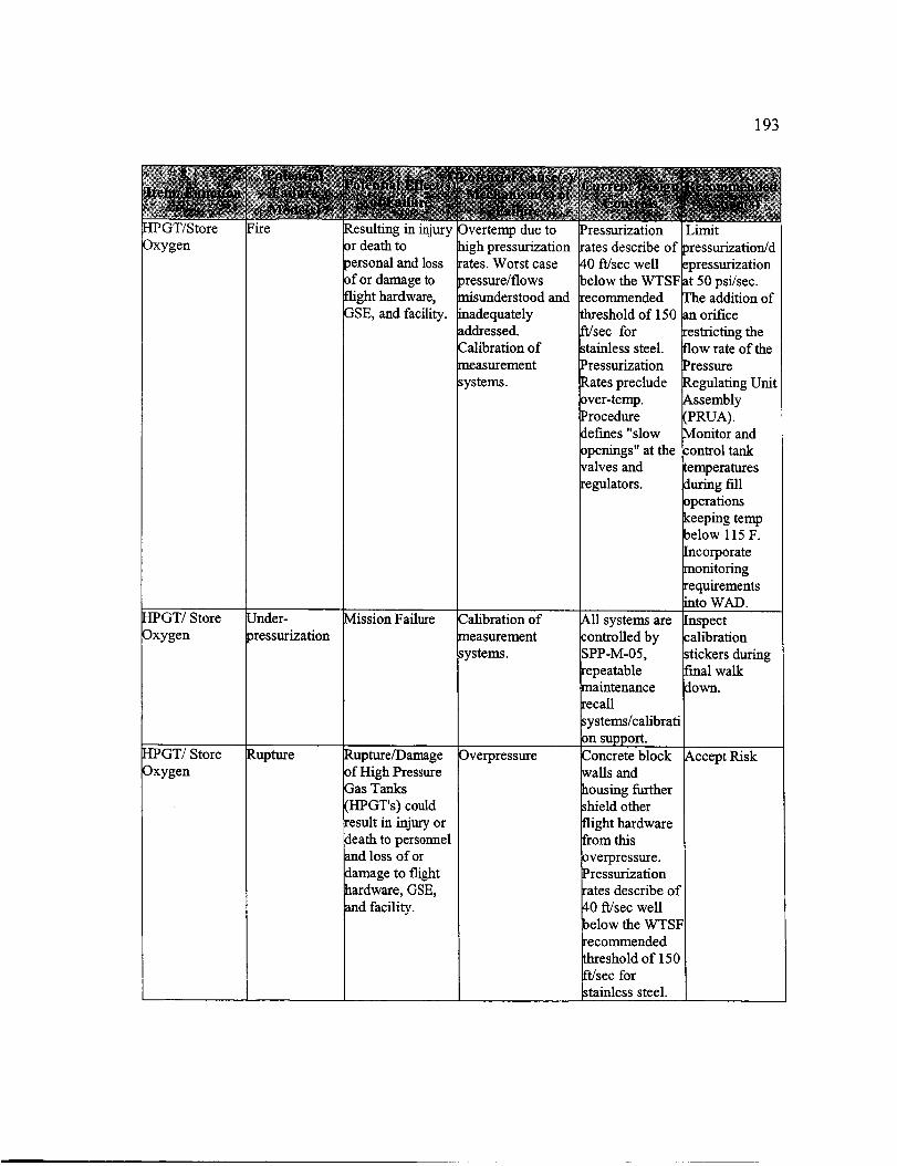
193
HPGT/StoreOxygen
Fire Resulting in injuryor death to
personal and loss
of or damage toflight hardware,
Dvertemp due toaigh pressurizationrates. Worst case
pressure/flowsmisunderstood and
Pressurizationrates describe of
40 ff/sec wellbelow the WTSF
recommended
HPGT/Store
Oxygen
HPGT/Store
Oxygen
Under-_ressurization
Rupture
GSE, and facility.
Mission Failure
Rupture/Damage
inadequately threshold of 150_ddressed. ft/sec for
Zalibration of stainless steel.
measurement Pressurization
_ystems. Rates preclude
over-temp.Procedure
defines "slow
openings" at thevalves and
regulators.
_alibration of All systems are
measurement controlled bysystems. SPP-M-05,
repeatablemaintenance
recall
systems/calibrati
m support.2oncrete blockOverpressure
of High PressureGas Tanks
(I-IPGT's) couldresult in injury ordeath to personnelmd loss of or
damage to flightaardware, GSE,
md facility.
_,alls and
aousing further;hield other
flight hardwarefrom this
3verpressure.Pressurization
rates describe of¢0 ft/sec well
below the WTSF
recommendedthreshold of 150
if/see for
_tainless steel.
Limit
pressurization/d
epressurizationat 50 psi/sec.The addition ofan orifice
restricting theflow rate of the
Pressure
Regulating Unit
Assembly(PRUA).Monitor and
:ontrol tank
:emperaturesduring fill_perations
,_eeping temp_elow 115 F.
Incorporate
monitoringrequirementsinto WAD.
Inspect:alibration
_tickers duringfinal walk
clown.
Accept Risk
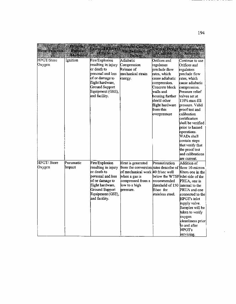
194
)xygen
{PGT/Store)xygen
resultingin injuryordeathto_ersonalandloss
CompressionReleaseofmechanicalstrain
Orificesandregulatorsprecludeflow
tes,whichofordamagetoflighthardware,GroundSupportEquipment(GSE),andfacility.
energy. :auseadiabatic"ompression.2oncrete blockwalls and
housing further_hield other
flight hardwarefrom this
_verpressure
?neumatic
ImpactFire/Explosion
resulting in injuryor death to
personal and lossof or damage toflight hardware,
3round SupportEquipment (GSE),
and facility.
Heat is generated_om the conversion
af mechanical work
when a gas is;ompressed from a
low to a high
pressure.
Pressurization
rates describe of40 ft/sec wellbelow the WTSF
recommendedthreshold of 150
ft/sec forstainless steel.
Drifices and
regulators_reclude flow
rates, whichzause adiabatic
_ompression.Pressure reliefvalves set at
110% max fill_ressure. Valid
_roof test andcalibration
certificationshall be verified
_rior to hazard
operations.WADs shall
contain stepsthat verify thatthe proof testand calibrationsare current.
.Addition of
_aree 10-micronfilters one in the
inlet side of the
PRUA, one isinternal to thePRUA and one
connected to theHPGT's inlet
supply valve.
Samples wiU betaken to verify
oxygencleanliness prioJto and afterHPGT's
servicing.

195
HPGT/Store
OxygenIgnition bymechanical
impact
?ire/Explosionresulting in injury3r death to
_ersonal and loss
ff or damage toflight hardware,
_round SupportEquipment (GSE),
_nd facility.
It has beendetermined forseveral aluminum
alloys that the
minimum energy toinduce samplefracture was less
than or equal to theminimum energy
required to induceignitions by
mechanical impact.Mechanical impacttesting of:ontaminated
mrfaces in oxygen_dicates an• lcrease in
_echanical impact
_ensitivity
iSpringer, 1975).
System layoutallows direct
verbal and visualcommunications
All operators are'
together, nonelocated
remotely.Communicationswith other O &
C will be_stablished
[f crane is at a
distant greaterthan 10 inchesfrom a structure
3peration speedhas to be less
than 2 in./min.Within 10-in.
operate less thanin./min.

APPENDIX J
Barrier Analysis for the KSC Project
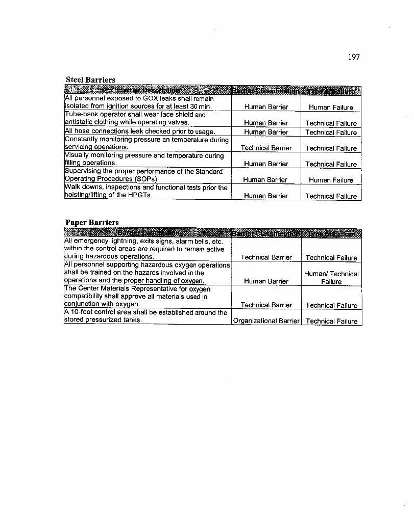
197
Steel Barriers
_:: ' :" _ _7_ _'_ ........ _, '_ ...... _':,;_ i .... _ _ •
All personnel exposed to GOX leaks shall remainisolated from ignition sources for at least 30 min.Tube-bank operator shall wear face shield andantistatic clothing while operating valves.
All hose connections leak checked prior to usage.Constantly monitoring pressure an temperature duringservicing operations.Visually monitoring pressure and temperature duringfilling operations.Supervising the proper performance of the StandardOperating Procedures (SOPs).Walk downs, inspections and functional tests prior thehoisting/lifting of the HPGTs.
Human Barrier
Human Barrier
Human Barrier
Human Failure
Technical FailureTechnical Failure
Technical Barrier Technical Failure
Human Barrier Technical Failure
Human Barrier
Human Barrier
Human Failure
Technical Failure
Paper Barriers
_11emergency lightning, exits signs, alarm bells, etc.within the control areas are required to remain activeduring hazardous operations. Technical Barrier Technical Failure_,11personnel supporting hazardous oxygen operationsshall be trained on the hazards involved in the3perations and the proper handling of oxygen.The Center Materials Representative for oxygen:ompatibility shall approve all materials used in:onjunction with oxygen._, 10-foot control area shall be established around thestored pressurized tanks.
Human Barrier
Technical Barrier
Organizational Barrier
Human/TechnicalFailure
Technical Failure
Technical Failure

APPENDIX K
Classification of Dendritics for the KSC Project

199
Failure to Adhere toStandard OperatingProcedure (SOP).
Protective coveringsaskew/leaking/corroded
Personnel locatedJnder suspended ormoving loads.
_)ver pressurization ofHPGTs.
Temperature exceeds3reset limits.Impact of structures witl"'.anks.Vlalfunctions in
;ompressor and pump"esulting in ignition and:ire.
Test being conductedess than 3 m (10 ft)Tom any opening inNails of adjacentstructures.
Testing being:onducted twenty-five:eet from any structurestcith fire-resistive_xterior walls orsprinkler buildings of_ther construction, butaot less than one-half',heheight of adjacentsidewall of the structure.
Testing being:onducted fifty feet from:;ombustible structures.
Test being conductedless than 15.2m (50ft)from solid materials thatburn rapidly, such asexcelsior or paper.
Reaching to HoistHPGT.
:Dperatorsengaging in3ractices that divertLheirattention while
3peratin 0 a Hoist.Instrumentationcalibration not done on-egular scheduledintervals.
Hose/tubing located inhigh-traffic area.
Misreading of portableoxygen monitor.
Discrepancies in gaugereadings.
Under pressurization of Spacing from suchHPGTs. structures is less than 1
foot preventingmaintenance.
Flow rates exceed Abnormal noise.3reset limits.General cleanliness. Unauthorized
)ersonnel.Contaminants in oxygen Failure to establishIank components, safety zones with
appropriate barriers(rope, cones, etc.) priorto lift.
Excessive vibration oflround support_quipment.
Full and emptycontainers storedLogether.
Incorrect valveoperation sequence.
Releasing GN2 into theO&C.
Operator not securingarea making sure thatthe area is clear of)ersonnel before
_tarting a hoist.
Personnel not wearingproper PersonalProtective Equipment(eeE).Personnel limitation fora test cell exceeded.
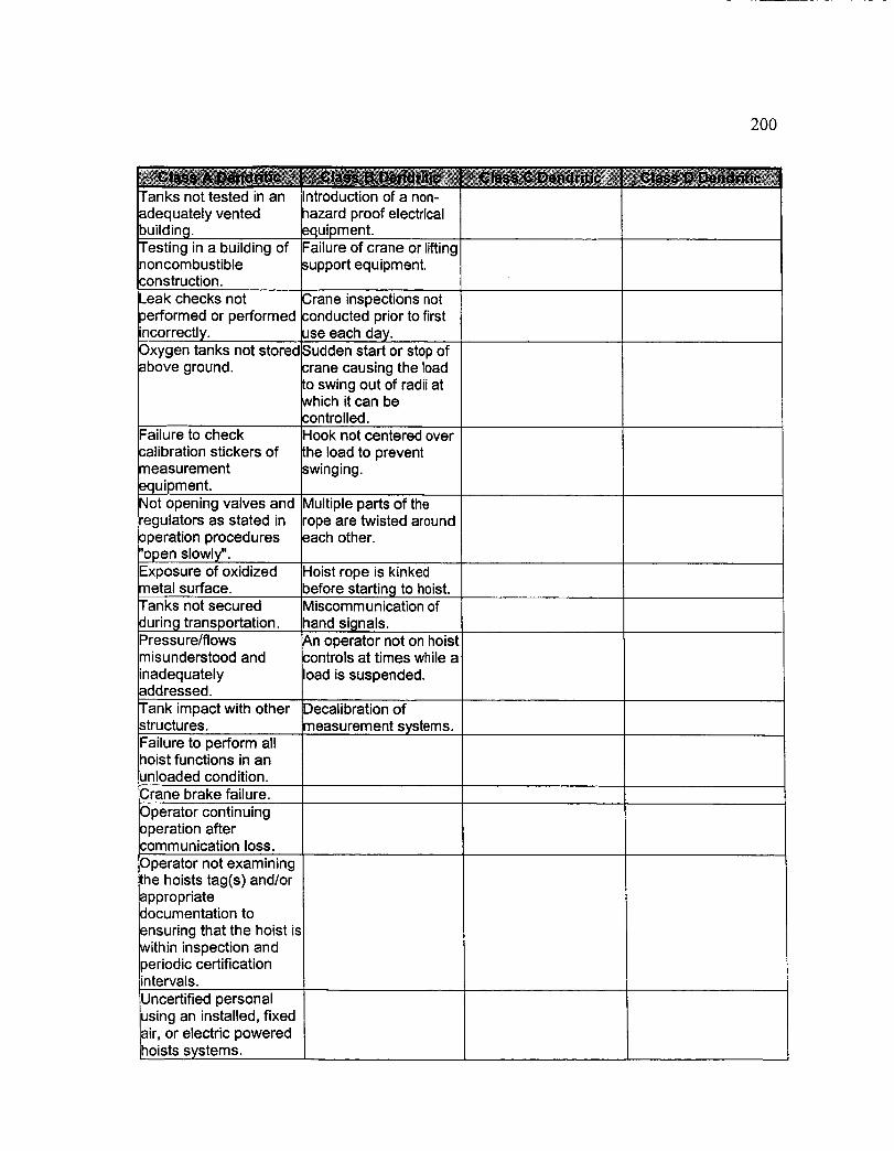
200
Tanks not tested in anadequately ventedt)uilding.Testing in a building ofnoncombustible=onstruction.Leak checks not3erformed or performedincorrectly.Oxygen tanks not storedabove ground.
Failure to check=alibration stickers ofmeasurement_=quipment.Not opening valves and"egulators as stated in3peration procedures'open slowly".Exposure of oxidizedmetal surface.Tanks not secured
durin9 transportation.Pressure/flowsmisunderstood andinadequatelyaddressed.
Tank impact with otherstructures.Failure to perform allhoist functions in anunloaded condition.Crane brake failure.Operator continuingoperation aftercommunication loss.Operator not examiningthe hoists tag(s) and/orappropriatedocumentation toensuring that the hoist iswithin inspection and)eriodic certificationintervals.
Uncertified personalusing an installed, fixedair, or electric poweredihoists systems.
Introduction of a non-_azard proof electrical_quipment.Failure of crane or liftingsupport equipment.
Crane inspections not=onducted prior to firstJse each day.Sudden start or stop of=rane causing the loadto swing out of radii atwhich it can be=ontrolled.Hook not centered overthe load to preventswinging.
Multiple parts of therope are twisted aroundeach other.
Hoist rope is kinkedbefore starting to hoist.Miscommunication of
hand signals.An operator not on hoistcontrols at times while aload is suspended.
Decalibration of
measurement systems.
APPENDIX L
c Control Chart Data for the KSC Project

2O2
Subgroupor
sample
Number of dendritics in observation h of sample i
3 1 1 1 0
4 1 0 0 0
5 0 1 0 0
6 0
7 0
8 0
9
10
11
12
13
0
0 O 0
1 0 0
0 0 2
0
Totalnumber of
dendritics insample i
4
4
3
1
1
O
1
2
5
5
5
3
1 0 2 4
14 2 1 1 0 4
15 1 1 0 0 2
16 1 0 0 0 1
17 1 0 O 1 2
18 0 0 1 1 2
APPENDIX M
Weighted Control Chart Data for the KSC Project
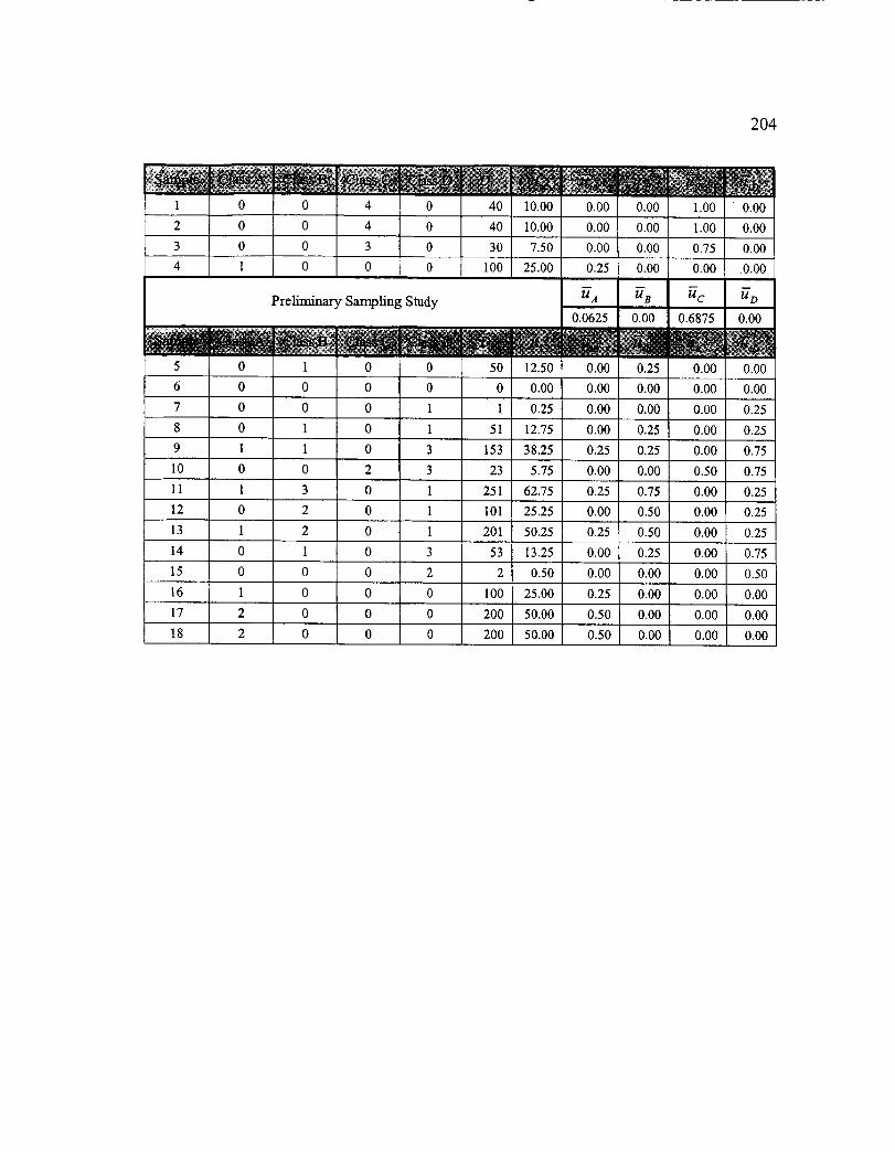
204
1 0 0 4 0 40 10.00
2 0 0 4 0 40 I0.00
3 0 0 3 0 30 7.50
4 1 0 0 0 100 25.00
Preliminary Sampling Study
,,, ,,,, l,
0.00 0.00 1.00 0.00
0.00 0.00 1.00 0.00
0.00 0.00 0.75 0.00
0.25 0.00 0.00 0.00
0.0625 0.00 0.6875 0.00
5 0 1 0 0 50 12.50 0.00 0.25 0.00 0.00
6 0 0 0 0 0 0.00 0.00 0.00 0.00 0.00
7 0 0 0 I 1 0.25 0.00 0.00 0.00 0.25
8 0 1 0 1 51 12.75 0.00 0.25 0.00 0.25
9 1 1 0 3 153 38.25 0.25 0.25 0.00 0.75
10 0 0 2 3 23 5.75 0.00 0.00 0.50 0.75
11 1 3 0 1 251 62.75 0.25 0.75 0.00 0.25
12 0 2 0 1 101 25.25 0.00 0.50 0.00 0.25
13 1 2 0 1 201 50.25 0.25 0.50 0.00 0.25
14 0 1 0 3 53 13.25 0.00 0.25 0.00 0.75
15 0 0 0 2 2 0.50 0.00 0.00 0.00 0.50
16 1 0 0 0 100 25.00 0.25 0.00 0.00 0.00
17 2 0 0 0 200 50.00 0.50 0.00 0.00 0.00
18 2 0 0 0 200 50.00 0.50 0.00 0.00 0.00