A review of hydrodynamic and energy-transport models … · A Review of Hydrodynamic and Energy-Transport Models for ... or from basic princi- ... A REVIEW OF HYDRODYNAMIC AND ENERGY-TRANSPORT

A Review of Hydrodynamic andEnergy-Transport Models for SemiconductorDevice Simulation

TIBOR GRASSER, TING-WEI TANG, FELLOW, IEEE, HANS KOSINA, MEMBER, IEEE, AND

SIEGFRIED SELBERHERR, FELLOW, IEEE

Contributed Paper

Since Stratton published his famous paper four decades ago, var-ious transport models have been proposed which account for theaverage carrier energy or temperature in one way or another. Theneed for such transport models arose because the traditionally useddrift-diffusion model cannot capture nonlocal effects which gainedincreasing importance in modern miniaturized semiconductor de-vices. In the derivation of these models from Boltzmann’s transportequation, several assumptions have to be made in order to obtaina tractable equation set. Although these assumptions may differsignificantly, the resulting final models show various similarities,which has frequently led to confusion. We give a detailed review onthis subject, highlighting the differences and similarities betweenthe models, and we shed some light on the critical issues associatedwith higher order transport models.

Keywords—Numerical analysis, semiconductor device mod-eling, simulation.

I. INTRODUCTION

At the very beginnings of semiconductor technology, theelectrical device characteristics could be estimated usingsimple analytical models relying on the drift-diffusion (DD)formalism. Various approximations had to be made to obtainclosed-form solutions, but the resulting models captured thebasic features of the devices. These approximations includesimplified doping profiles and device geometries. With theongoing refinements and improvements in technology, theseapproximations lost their basis and a more accurate descrip-

Manuscript received January 3, 2002; revised July 2, 2002. This work wassupported in part by the Christian Doppler Forschungsgesellschaft, Vienna,Austria, and in part by the National Science Foundation under Grant ECS-0120128.

T. Grasser, H. Kosina, and S. Selberherr are with the Institute for Micro-electronics, Technical University Vienna, A-1040 Vienna, Austria (e-mail:[email protected]).

T.-W. Tang is with the Department of Electrical and Computer Engi-neering, University of Massachusetts, Amherst, MA 01003 USA (e-mail:[email protected]).

Digital Object Identifier 10.1109/JPROC.2002.808150

tion was required. This goal could be achieved by solvingthe DD equations numerically. Numerical simulation ofcarrier transport in semiconductor devices dates back to thefamous work of Scharfetter and Gummel [1], who proposeda robust discretization of the DD equations which is still inuse today.

However, as semiconductor devices were scaled intothe submicrometer regime, the assumptions underlyingthe DD model lost their validity. Therefore, the transportmodels have been continously refined and extended tomore accurately capture transport phenomena occurringin these submicrometer devices. The need for refinementand extension is primarily caused by the ongoing featuresize reduction in state-of-the-art technology. As the supplyvoltages cannot be scaled accordingly without jeopardizingthe circuit performance, the electric field inside the deviceshas increased. A large electric field which rapidly changesover small length scales gives rise to nonlocal and hot-carriereffects which begin to dominate device performance. Anaccurate description of these phenomena is required and isbecoming a primary concern for industrial applications.

To overcome some of the limitations of the DD model,extensions have been proposed which basically add an ad-ditional balance equation for the average carrier energy [2],[3]. Furthermore, an additional driving term is added to thecurrent relation which is proportional to the gradient of thecarrier temperature. However, a vast number of these modelsexists, and there is a considerable amount of confusion as totheir relation to each other. The aim of this paper is to clarifythe important differences and similarities between the var-ious models. To master this task, a closer look at the variousderivations is required, where the important points are high-lighted. Then the most important models are summarized andassessed, followed by a critical discussion of the assumptionsmade in the derivation.

0018-9219/03$17.00 © 2003 IEEE

PROCEEDINGS OF THE IEEE, VOL. 91, NO. 2, FEBRUARY 2003 251

II. THE DRIFT-DIFFUSION MODEL

The DD model is the simplest current transport modelwhich can be derived from Boltzmann’s transport equation(BTE) by the method of moments [4] or from basic princi-ples of irreversible thermodynamics [5]. For many decades,the DD model has been the backbone of semiconductor de-vice simulation. In this model, the electron current density isphenomenologically expressed as consisting of two compo-nents. The drift component is driven by the electric field andthe diffusion component by the electron density gradient. Itis given by

(1)

where and are the mobility and the diffusivity of theelectron gas, respectively, and are related to each other bythe Einstein relation

(2)

where is the Boltzmann constant. The current relation (1)is inserted into the continuity equation

(3)

to give a second-order parabolic differential equation, whichis then solved together with Poisson’s equation. Note thatgeneration/recombination effects were neglected in (3).

In the DD approach, the electron gas is assumed to be inthermal equilibrium with the lattice temperature .However, in the presence of a strong electric field, electronsgain energy from the field and the temperature of the elec-tron gas is elevated. Since the pressure of the electrongas is proportional to , the driving force now becomesthe pressure gradient rather then merely the density gradient.This introduces an additional driving force, namely, the tem-perature gradient besides the electric field and the densitygradient. Phenomenologically, one can write

(4)

where is the thermal diffusivity.Although the DD equations are based on the assumption

that the electron gas is in thermal equilibrium with the lattice,an estimation for the local temperature can be calculated withthe local energy balance equation [6]

(5)

where is the energy relaxation time. Equation (5) isobtained under the assumption of a local energy balance.At the critical electric field , which depends on the electricfield via the mobility, the carrier temperature reaches twicethe value of the lattice temperature. is in the orderof 10 kV/cm, a value easily exceeded even in not veryadvanced devices where values higher than 1 MV/cm canbe observed [7]. Note too that the temperature obtained

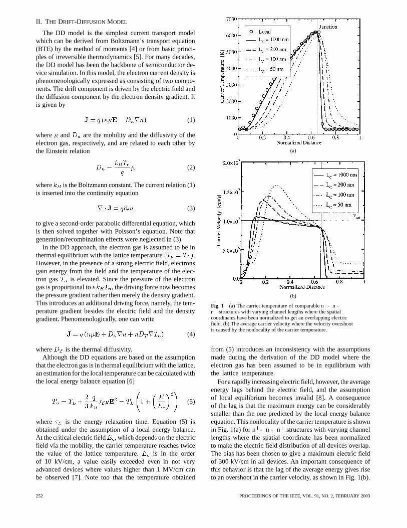
(a)

(b)

Fig. 1 (a) The carrier temperature of comparable n- n -n structures with varying channel lengths where the spatialcoordinates have been normalized to get an overlapping electricfield. (b) The average carrier velocity where the velocity overshootis caused by the nonlocality of the carrier temperature.

from (5) introduces an inconsistency with the assumptionsmade during the derivation of the DD model where theelectron gas has been assumed to be in equilibrium withthe lattice temperature.

For a rapidly increasing electric field, however, the averageenergy lags behind the electric field, and the assumptionof local equilibrium becomes invalid [8]. A consequenceof the lag is that the maximum energy can be considerablysmaller than the one predicted by the local energy balanceequation. This nonlocality of the carrier temperature is shownin Fig. 1(a) for n - n - n structures with varying channellengths where the spatial coordinate has been normalizedto make the electric field distribution of all devices overlap.The bias has been chosen to give a maximum electric fieldof 300 kV/cm in all devices. An important consequence ofthis behavior is that the lag of the average energy gives riseto an overshoot in the carrier velocity, as shown in Fig. 1(b).

252 PROCEEDINGS OF THE IEEE, VOL. 91, NO. 2, FEBRUARY 2003

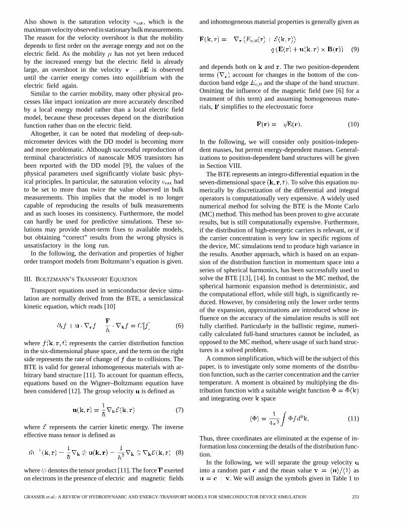
Also shown is the saturation velocity , which is themaximumvelocityobserved instationarybulkmeasurements.The reason for the velocity overshoot is that the mobilitydepends to first order on the average energy and not on theelectric field. As the mobility has not yet been reducedby the increased energy but the electric field is alreadylarge, an overshoot in the velocity is observeduntil the carrier energy comes into equilibrium with theelectric field again.

Similar to the carrier mobility, many other physical pro-cesses like impact ionization are more accurately describedby a local energy model rather than a local electric fieldmodel, because these processes depend on the distributionfunction rather than on the electric field.

Altogether, it can be noted that modeling of deep-sub-micrometer devices with the DD model is becoming moreand more problematic. Although successful reproduction ofterminal characteristics of nanoscale MOS transistors hasbeen reported with the DD model [9], the values of thephysical parameters used significantly violate basic phys-ical principles. In particular, the saturation velocity hadto be set to more than twice the value observed in bulkmeasurements. This implies that the model is no longercapable of reproducing the results of bulk measurementsand as such looses its consistency. Furthermore, the modelcan hardly be used for predictive simulations. These so-lutions may provide short-term fixes to available models,but obtaining “correct” results from the wrong physics isunsatisfactory in the long run.

In the following, the derivation and properties of higherorder transport models from Boltzmann’s equation is given.

III. B OLTZMANN’S TRANSPORTEQUATION

Transport equations used in semiconductor device simu-lation are normally derived from the BTE, a semiclassicalkinetic equation, which reads [10]

(6)

where represents the carrier distribution functionin the six-dimensional phase space, and the term on the rightside represents the rate of change ofdue to collisions. TheBTE is valid for general inhomogeneous materials with ar-bitrary band structure [11]. To account for quantum effects,equations based on the Wigner–Boltzmann equation havebeen considered [12]. The group velocityis defined as

(7)

where represents the carrier kinetic energy. The inverseeffective mass tensor is defined as

(8)

where denotes the tensor product [11]. The forceexertedon electrons in the presence of electric and magnetic fields

and inhomogeneous material properties is generally given as

(9)

and depends both on and . The two position-dependentterms account for changes in the bottom of the con-duction band edge and the shape of the band structure.Omitting the influence of the magnetic field (see [6] for atreatment of this term) and assuming homogeneous mate-rials, simplifies to the electrostatic force

(10)

In the following, we will consider only position-indepen-dent masses, but permit energy-dependent masses. General-izations to position-dependent band structures will be givenin Section VIII.

The BTE represents an integro-differential equation in theseven-dimensional space . To solve this equation nu-merically by discretization of the differential and integraloperators is computationally very expensive. A widely usednumerical method for solving the BTE is the Monte Carlo(MC) method. This method has been proven to give accurateresults, but is still computationally expensive. Furthermore,if the distribution of high-energetic carriers is relevant, or ifthe carrier concentration is very low in specific regions ofthe device, MC simulations tend to produce high variance inthe results. Another approach, which is based on an expan-sion of the distribution function in momentum space into aseries of spherical harmonics, has been successfully used tosolve the BTE [13], [14]. In contrast to the MC method, thespherical harmonic expansion method is deterministic, andthe computational effort, while still high, is significantly re-duced. However, by considering only the lower order termsof the expansion, approximations are introduced whose in-fluence on the accuracy of the simulation results is still notfully clarified. Particularly in the ballistic regime, numeri-cally calculated full-band structures cannot be included, asopposed to the MC method, where usage of such band struc-tures is a solved problem.

A common simplification, which will be the subject of thispaper, is to investigate only some moments of the distribu-tion function, such as the carrier concentration and the carriertemperature. A moment is obtained by multiplying the dis-tribution function with a suitable weight functionand integrating over space

(11)

Thus, three coordinates are eliminated at the expense of in-formation loss concerning the details of the distribution func-tion.

In the following, we will separate the group velocityinto a random part and the mean value as

. We will assign the symbols given in Table 1 to

GRASSERet al.: A REVIEW OF HYDRODYNAMIC AND ENERGY-TRANSPORT MODELS FOR SEMICONDUCTOR DEVICE SIMULATION 253

the moments of the distribution function [15]. Furthermore,we will employ an isotropic effective mass approximationvia the trace of the mass tensor [16]

(12)

IV. BAND STRUCTURE

A common assumption in macroscopic transport modelsis that the band structure is isotropic; that is, the kinetic en-ergy depends only on the magnitude of the wave vector.With this assumption, the dispersion relation can be writtenin terms of the band form function

(13)

The simplest approximation for the real band structure is aparabolic relationship between the energy and the carrier mo-mentum

(14)

which is assumed to be valid for energies close to the bandminimum. A first-order nonparabolic relationship was givenby Kane [17]

(15)

with being the nonparabolicity correction factor. Kane’sdispersion relation gives the following relationship betweenmomentum and velocity:

(16)

Therefore, the average velocity contains an infinite numberof higher order terms which are not necessarily negligible.This is problematic because these quantities are additionalunknowns representing higher order moments of the velocitydistribution which prohibits closed-form solutions.

To obtain a more tractable expression, Cassi and Riccò[18] approximated Kane’s dispersion relation as

(17)

and fitted the parametersand for different energy ranges.For , the conventional parabolic dispersion relationis obtained. As pointed out in [19], this expression must beused with care. In particular, physically meaningful resultscould be obtained only by fitting (17) to the energy range

eV . This can be explained by looking more closely atthe density of states, which is obtained as

(18)

and in the particular case of Cassi’s model

(19)

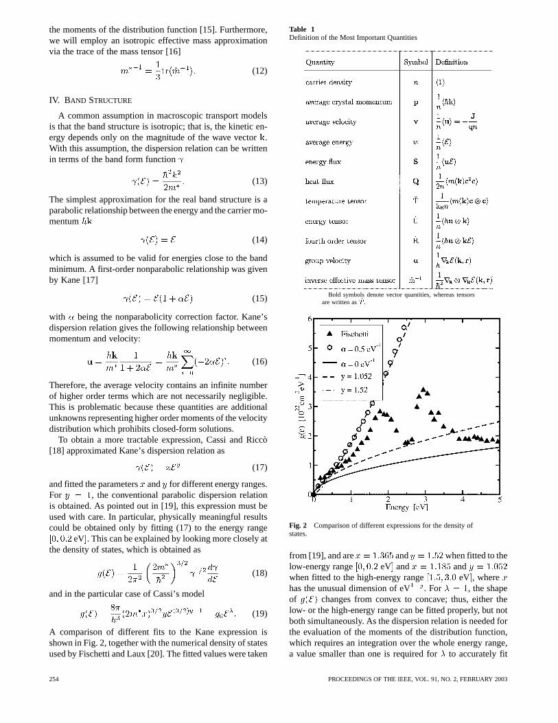
A comparison of different fits to the Kane expression isshown in Fig. 2, together with the numerical density of statesused by Fischetti and Laux [20]. The fitted values were taken

Table 1Definition of the Most Important Quantities

Bold symbols denote vector quantities, whereas tensorsare written as .

Fig. 2 Comparison of different expressions for the density ofstates.

from [19], and are and when fitted to thelow-energy range eV and andwhen fitted to the high-energy range eV , wherehas the unusual dimension of eV . For , the shapeof changes from convex to concave; thus, either thelow- or the high-energy range can be fitted properly, but notboth simultaneously. As the dispersion relation is needed forthe evaluation of the moments of the distribution function,which requires an integration over the whole energy range,a value smaller than one is required forto accurately fit


the low-energy region because this is where has itsmaximum. However, the resulting density of states showsa “parabolic-like” behavior; therefore, it is of limited valuefor the description of nonparabolic transport phenomena.

V. DERIVATION OF HIGHER ORDERTRANSPORTMODELS

In this section, the basic steps for transforming BTE intoa macroscopic transport model will be reviewed to point outthe principal differences among the models. Generation andrecombination processes are not considered in the following.

A. Stratton’s Approach

One of the first derivations of extended transport equationswas performed by Stratton [2]. First, the distribution functionis split into the even and odd parts

(20)

From , it follows that . As-suming that the collision operator is linear and invoking amicroscopic relaxation time approximation for the collisionoperator

(21)

the BTE can be split into two coupled equations. In partic-ular, is related to via

(22)

The microscopic relaxation time is then expressed by a powerlaw

(23)

When is assumed to be a heated Maxwellian distribution,the following equation system is obtained:

(24)

(25)

(26)

(27)

Equation (25) can be rewritten as

(28)

with

(29)

which is commonly used as a fit parameter with values in therange . For , the thermal diffusion

term disappears. Under certain assumptions [2], [21], the co-efficient equals . The problem with expression (23) for

is that must be approximated by an average value to coverthe relevant scattering processes. In the particular case of im-purity scattering, can be in the range , dependingon charge screening [22]. Therefore, this average depends onthe doping profile and the applied field; thus, no unique valuefor can be given.

Note that the temperature which appears in (24)–(27)is a parameter of the heated Maxwellian distribution, whichhas been assumed in the derivation. Only for parabolic bandsand a Maxwellian distribution, this parameter is equivalent tothe normalized second-order moment.

B. Bløtekjær’s Approach

Bløtekjær [3] derived conservation equations by taking themoments of the BTE using the weight functions one,, and

without imposing any assumptions on the form of the dis-tribution function. These weight functionsdefine the mo-ments of zeroth, first, and second order. The resulting mo-ment equations can be written as follows [15]:

(30)

(31)

(32)

These expressions are valid for arbitrary band structures,provided that the carrier mass is position independent.When is allowed to be position dependent, additionalforce terms appear in (30)–(32) [23]. The collision terms areusually modeled employing a macroscopic relaxation timeapproximation as

(33)

(34)

(35)

which introduces the momentum and energy relaxationtimes and , respectively. A discussion on this approx-imation is given in [24]. One should note the differencebetween themicroscopicrelaxation time approximation asused by Stratton, where the whole scattering operator is ap-proximated by a single relaxation time, and themacroscopicrelaxation time approximation, where a separate relaxationtime is introduced for every moment of the scatteringoperator. The latter is assumed to be more accurate.

This equation set is not closed, as it contains more un-knowns than equations. Closure relations have to be foundto express the equations in terms of the unknowns, , and

. Traditionally, parabolic bands are assumed, which givesthe following closure relations for, , and :

(36)

(37)

(38)


The random component of the velocity has zero average, thatis, . Under the assumption that the distribution func-tion is isotropic, the following relation can be derived:

(39)

This assumption is frequently considered to be justified be-cause of the strong influence of scattering. Approximatingby a scalar temperature as

(40)

(37) and (38) become coupled

(41)

(42)

With (34) and (36), one obtains the following formulationfor :

(43)

where and have been lumped into one new parameter,the mobility

(44)

Relationship (44) is valid for parabolic bands only, whereasfor arbitrary bands the mobility can be defined directly viathe collision term. As signal frequencies are well below

Hz, the time derivative in (31) can safelybe neglected [25].

Furthermore, a suitable approximation for the energy fluxdensity has to be found, and different approaches havebeen published. Bløtekjær used

(45)

and approximated the heat flux by Fourier’s law as

(46)

in which the thermal conductivity is given by the Wiede-mann–Franz law as

(47)

where is a correction factor. The artificial introduction ofwas based on physical reasoning only because a shifted andheated Maxwellian distribution gives . This is a majorinconsistency of the model. In addition, as has been pointedout in [15], this expression is problematic, as (46) only ap-proximates the diffusive component of . For a uniformtemperature, ; thus, , which contradicts withMC simulations. The convective component must beincluded to obtain physical results when the current flow isnot negligible.

With these approximations, (30)–(32) can be written in theusual variables as [26]

(48)

(49)

(50)

(51)

to give the full hydrodynamic model (FHD) for parabolicband structures, which has been supplemented by the phe-nomenological constitutive relation (51) to close the system.This equation system is similar to the Euler equations of fluiddynamics with the addition of a heat conduction term and thecollision terms. It describes the propagation of electrons in asemiconductor device as the flow of a compressible, chargedfluid. This electron gas has a sound speed ,and the electron flow may be either subsonic or supersonic.With and K, cm/s,while for K, cm/s [27]. In thecase of supersonic flow, electron shock waves will in gen-eral develop inside the device. These shock waves occur ateither short-length scales or low temperatures. As the equa-tion system is hyperbolic in the supersonic regions, specialnumerical methods have to be used (see Section XIII) whichare not compatible to the methods employed for the parabolicconvection-diffusion type of equations.

When the convective term in the current relation (49)

(52)

is neglected, a parabolic equation system is obtainedwhich covers only the subsonic flow regions. This is avery common approximation in today’s device simulators.Furthermore, the contribution of the velocity to the carrierenergy is frequently neglected, resulting in

(53)

The two assumptions made previously can be justified from amathematical point of view because they follow consistentlyfrom appropriately scaling the BTE. The Knudsen numberappears as a scaling parameter, which represents the meanfree path relative to the device dimension [28]

(54)

where is the characteristic time between scattering events,denotes the velocity scale, and is given by the size of

the simulation domain. Carriers in a semiconductor at roomtemperature can be considered a collision-dominated system,for which . Diffusion scaling assumes the time scaleof the system to be

(55)

In the limit of vanishing Knudsen number, , oneobtains that convective terms of the form are ne-glected against . The consequences are that the drift


kinetic energy is neglected against , and thatin the flux equations the time derivatives vanish.

The resulting simplified equations are

(56)

(57)

(58)

(59)

Equations (56) and (59) form a typical three-moment modelwhich has been closed using Fourier’s law and is commonlyknown in the literature as the energy-transport (ET) model.Actually, this name is misleading, as the model consists ofthe two conservation equations (56) and (58) and the twoconstitutive equations (57) and (59).

To overcome the difficulties associated with the Fourierlaw closure (46), the fourth moment of the BTE has beentaken into account, [15] which gives

(60)

The time derivative is ignored using the same scaling argu-ment that led to neglecting the time derivative in (31). Thecollision term in (60) can be modeled in analogy to (43) as

(61)

which gives

(62)

Now a closure relation for has to be introduced, which canbe, for example, obtained by assuming a heated Maxwelliandistribution. This gives

(63)

Using closure (63) and the same approximations that led tothe three-moments ET model (56)–(59), a more accurate ex-pression for is obtained from the fourth moment of theBTE

(64)

which should be used to replace (59) to give a four-momentsET model. Comparing (64) with (59) reveals the inconsis-tency of the three-moments ET model. In the four-momentsmodel, we have the factor

(65)

for both terms. In the three-moments model, however, thefactors are and , which means that the heat fluxcan be adjusted independently. This inconsistency can beavoided only if and . However, the ratio

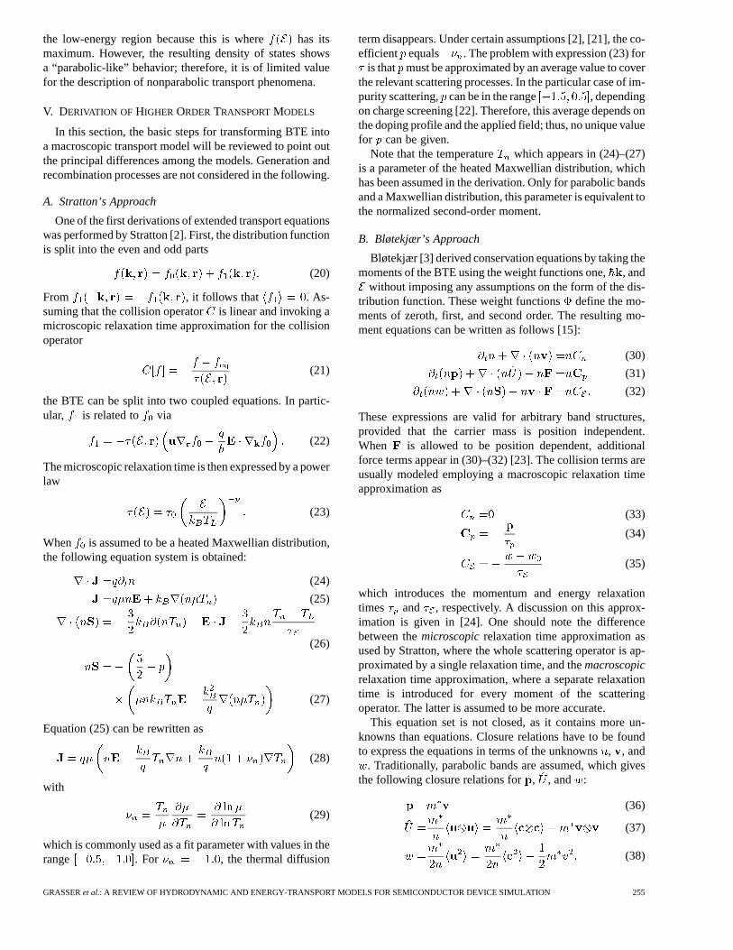
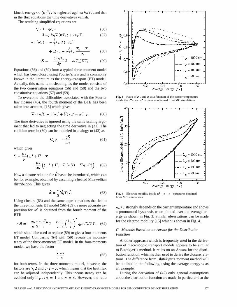
Fig. 3 Ratio of� and� as a function of the carrier temperatureinside the n - n - n structures obtained from MC simulations.

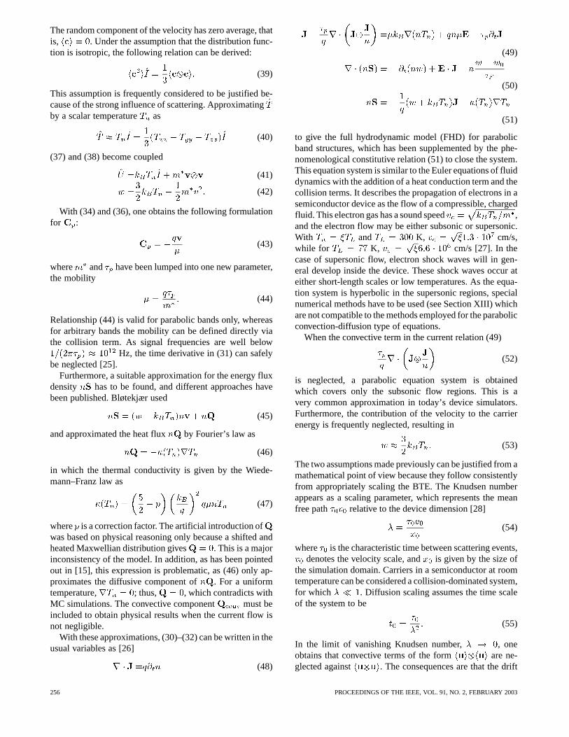
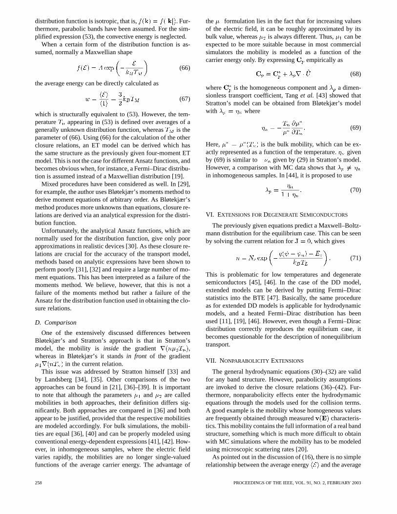
Fig. 4 Electron mobility inside n - n - n structures obtainedfrom MC simulations.

strongly depends on the carrier temperature and showsa pronounced hysteresis when plotted over the average en-ergy as shown in Fig. 3. Similar observations can be madefor the electron mobility [15] which is shown in Fig. 4.

C. Methods Based on an Ansatz for the DistributionFunction

Another approach which is frequently used in the deriva-tion of macroscopic transport models appears to be similarto Bløtekjær’s method. It relies on an Ansatz for the distri-bution function, which is then used to derive the closure rela-tions. The difference from Bløtekjær’s moment method willbe outlined in the following, using the average energyasan example.

During the derivation of (42) only general assumptionsabout the distribution function are made, in particular that the


distribution function is isotropic, that is, . Fur-thermore, parabolic bands have been assumed. For the sim-plified expression (53), the convective energy is neglected.

When a certain form of the distribution function is as-sumed, normally a Maxwellian shape

(66)

the average energy can be directly calculated as

(67)

which is structurally equivalent to (53). However, the tem-perature appearing in (53) is defined over averages of agenerally unknown distribution function, whereas is theparameter of (66). Using (66) for the calculation of the otherclosure relations, an ET model can be derived which hasthe same structure as the previously given four-moment ETmodel. This is not the case for different Ansatz functions, andbecomes obvious when, for instance, a Fermi–Dirac distribu-tion is assumed instead of a Maxwellian distribution [19].

Mixed procedures have been considered as well. In [29],for example, the author uses Bløtekjær’s moments method toderive moment equations of arbitrary order. As Bløtekjær’smethod produces more unknowns than equations, closure re-lations are derived via an analytical expression for the distri-bution function.

Unfortunately, the analytical Ansatz functions, which arenormally used for the distribution function, give only poorapproximations in realistic devices [30]. As these closure re-lations are crucial for the accuracy of the transport model,methods based on analytic expressions have been shown toperform poorly [31], [32] and require a large number of mo-ment equations. This has been interpreted as a failure of themoments method. We believe, however, that this is not afailure of the moments method but rather a failure of theAnsatz for the distribution function used in obtaining the clo-sure relations.

D. Comparison

One of the extensively discussed differences betweenBløtekjær’s and Stratton’s approach is that in Stratton’smodel, the mobility is inside the gradient ,whereas in Bløtekjær’s it standsin front of the gradient

in the current relation.This issue was addressed by Stratton himself [33] and

by Landsberg [34], [35]. Other comparisons of the twoapproaches can be found in [21], [36]–[39]. It is importantto note that although the parameters and are calledmobilities in both approaches, their definition differs sig-nificantly. Both approaches are compared in [36] and bothappear to be justified, provided that the respective mobilitiesare modeled accordingly. For bulk simulations, the mobili-ties are equal [36], [40] and can be properly modeled usingconventional energy-dependent expressions [41], [42]. How-ever, in inhomogeneous samples, where the electric fieldvaries rapidly, the mobilities are no longer single-valuedfunctions of the average carrier energy. The advantage of

the formulation lies in the fact that for increasing valuesof the electric field, it can be roughly approximated by itsbulk value, whereas is always different. Thus, can beexpected to be more suitable because in most commercialsimulators the mobility is modeled as a function of thecarrier energy only. By expressing empirically as

(68)

where is the homogeneous component anda dimen-sionless transport coefficient, Tanget al. [43] showed thatStratton’s model can be obtained from Bløtekjær’s modelwith where

(69)

Here, is the bulk mobility, which can be ex-actly represented as a function of the temperature.givenby (69) is similar to given by (29) in Stratton’s model.However, a comparison with MC data shows thatin inhomogeneous samples. In [44], it is proposed to use

(70)

VI. EXTENSIONS FORDEGENERATESEMICONDUCTORS

The previously given equations predict a Maxwell–Boltz-mann distribution for the equilibrium case. This can be seenby solving the current relation for , which gives

(71)

This is problematic for low temperatures and degeneratesemiconductors [45], [46]. In the case of the DD model,extended models can be derived by putting Fermi–Diracstatistics into the BTE [47]. Basically, the same procedureas for extended DD models is applicable for hydrodynamicmodels, and a heated Fermi–Dirac distribution has beenused [11], [19], [46]. However, even though a Fermi–Diracdistribution correctly reproduces the equilibrium case, itbecomes questionable for the description of nonequilibriumtransport.

VII. N ONPARABOLICITY EXTENSIONS

The general hydrodynamic equations (30)–(32) are validfor any band structure. However, parabolicity assumptionsare invoked to derive the closure relations (36)–(42). Fur-thermore, nonparabolicity effects enter the hydrodymamicequations through the models used for the collision terms.A good example is the mobility whose homogeneous valuesare frequently obtained through measured characteris-tics. This mobility contains the full information of a real bandstructure, something which is much more difficult to obtainwith MC simulations where the mobility has to be modeledusing microscopic scattering rates [20].

As pointed out in the discussion of (16), there is no simplerelationship between the average energyand the average


velocity in the general case. For parabolic bands, the car-rier temperature is normally defined via the average carrierenergy as

(72)

Unfortunately, there is no similar equation for nonparabolicbands. Another possibility is to define the temperature viathe variance of the velocity as [16]

(73)

Definitions (72) and (73) are consistent with the thermody-namic definition of the carrier temperature in thermodynamicequilibrium, and both are identical for nonequilibrium caseswhen a constant carrier mass is assumed, which in turn cor-responds to the assumption of parabolic energy bands. How-ever, large differences are observed when a more realisticband structure is considered [16], [48].

A. The Generalized Hydrodynamic Model

Thoma et al. [16], [48] proposed a model which theytermed the generalized hydrodynamic model. Instead ofusing the average energyand the temperature as variablesin their formulation, they opted for a temperature-onlydescription. To obtain a form similar to standard models,they defined the temperature according to (73), which differssignificantly from (72) for nonparabolic bands. Instead ofthe momentum-based weight functions and , theyused the velocity-based weight functionsand to derivethe moment equations of order one and three. Withoutassuming any particular dispersion relation, they derived thefollowing equations for the current and energy flux density:

(74)

(75)

(76)

All relaxation times and mobilities are modeled as a func-tion of , and explicit formulas were given in [49]. The ad-vantage of this formulation is that it can be applied to arbi-trary band structures. Thomaet al., however, used parame-ters extracted from MC simulations employing Kane’s dis-persion relation. As these parameters are extracted from ho-mogeneous MC simulations, their validity for realistic de-vices is still an open issue. In a recent investigation [50],the relaxation times were calculated from full-band MC bulksimulations. Good agreement of transit-times of SiGe het-erostructure bipolar transistors was observed in comparisonwith full-band MC simulations.

B. Model of Bordelon et al.

Bordelonet al. [51], [52] proposed a nonparabolic modelbased on Kane’s dispersion relation. As weight functions,they used one, , and , and closed the system by ignoring

the heat flux. To avoid the problem with the missing energy-temperature relation, they formulated their equation systemsolely in . Their model is based on two assumptions: first,they assumed that the diffusion approximation holds. Re-garding the energy tensor, this allows for the following ap-proximation:

(77)

where Kane’s relation has been used. The problem is now toexpress the right side of (77) by available moments withoutintroducing new unknowns. This is not exactly possible, andthe approximation

(78)

has been introduced. Defining ,they obtained

(79)

(80)

with . In the comparison made in [38], the pre-dicted and curves agree quite well with the MC data,even with this simplified model for .

C. Model of Chen et al.

In [53], Chenet al.published a model which they termedthe improved energy transport model. They tried to includenonparabolic and non-Maxwellian effects to a first order.Their approach is based on Stratton’s, the use of Kane’s dis-persion relation, and an Ansatz for the distribution function

(81)

which contains a non-Maxwellian factor. They give thefollowing equations:

(82)

(83)

with

(84)

(85)

Interestingly, the non-Maxwellian factordoes not show upin the final equations. Sadovnikovet al. [49] showed thatChen’s model shows some weakness in predicting proper ve-locity profiles and is not consistent with homogeneous sim-ulation results.

D. Model of Tang et al.

This model is based on Kane’s dispersion relation andtakes particular care of correctly handling the inhomogeneityeffects, which are commonly ignored [43]. By observing that

and show nearly no hysteresis


when plotted against the average energy for several n- n- n structures, Tanget al. proposed the following closurerelations:

(86)

(87)

(88)

with and being single-valued fit functions. Theuse of Kane’s dispersion relation for the MC simulationmight limit the validity of the preceding expressions. Un-fortunately, the additional convective terms are difficultto handle and cause numerical problems [54]. Therefore,simplified expressions have been given in [55].

E. Model of Smith and Brennan

Smith and Brennan [19] derived two nonparabolic equa-tion sets for inhomogeneous and degenerate semiconductors(see also [56], [57]). They used both Kane’s dispersion rela-tion and the power-law approximation after Cassi and Riccò[18] because the former cannot be integrated analytically.Furthermore, they used Fermi–Dirac statistics to includedegeneracy effects. They showed that the typically em-ployed binomial expansion of the Kane integrands loses itsvalidity, and physically inconsistent results are obtained. Thepower-law approximation, on the other hand, approachesthe parabolic limit and has a larger range of validity.

Their approach has two drawbacks: first, as pointed outpreviously, Cassi’s density of states (19) cannot capture thenonparabolic nature of the bands; therefore, it is of limiteduse for a nonparabolic transport model. The authors them-selves noted that for , incorrect transport coefficientsare obtained. Therefore, they obtained the parameterby afit to the low energy range eV of Kane’s dispersion re-lation. As can be seen in Fig. 2, this gives near-parabolic be-havior of the density of states. Second, a heated Fermi–Diracstatistics provides no improvement over a heated Maxwellstatistic in terms of hot-carrier transport.

F. Model of Anile et al.

Anile and Romano [58] and Muscato [59] derivedclosed-form expressions for the closureand using anAnsatz for the distribution function based on the maximumentropy principle. In addition, they were able to deriveexpressions for the collision terms. They found that theirmodel fulfills Onsager’s reciprocity principle and gave acomparison with other hydrodynamic models which violatethe principle. Although Anile’s model has a sound physicalbasis, it is of limited practical use. Despite its complicatednature, the model is based on an analytical expressionfor the distribution function, which was assumed to be ofMaxwellian shape. Extended models were given in, e.g.,[60]. Note, however, that Onsager’s reciprocity theoremis valid only near equilibrium, a condition significantlyviolated in today’s semiconductor devices [61], [62].

G. Comparison

The use of more realistic band structure models than theparabolic band approximation adds severe complications tomacroscopic transport models. Even for the rather simpleKane dispersion relation, no closed-form equations can begiven. Therefore, all models rely on more or less severe ap-proximations. Whereas Thoma’s model is applicable for gen-eral band structures, Tang’s models attempt to capture non-local effects. A comparison of the simple ET model with theexpressions given by Thoma, Lee, Chen, and Tang for siliconbipolar transistors is given by Sadovnikovet al. [49], wheregood agreement with MC data was obtained for the modelsof Thoma and Tang.

VIII. E XTENSIONS FORSEMICONDUCTORALLOYS

The derivations given previously are restricted to homo-geneous materials where the effective carrier masses andthe band edge energies do not depend on position. Over thelast few years, extensive research has been made concerningcompound semiconductors where the inclusion of thecarrier temperature in the transport equations is generallyconsidered a must. To properly account for the additionaldriving forces due to changes in the effective masses andthe band edge energies, the ET models have been extendedaccordingly. The foundation for these extensions was laid inthe pioneering work by Marshak for the DD equations [47],[63]. These concepts have been applied to the ET models byAzoff [11], [23], [64]. In the case of a position-dependentparabolic band structure, the force exerted on an electron isgiven as

(89)

These additional forces give rise to an additional componentin the current relation, and the electric field is replaced by aneffective electric field which also contains the gradient of theband edges

(90)

(91)

An extension to nonparabolic band structures has been pre-sented by Smithet al. [19], [56].

IX. M ULTIPLE BAND MODELS

Bløtekjær’s [3] equations were originally devisedfor semiconductors with multiple bands. Woolardet al.[65]–[67] extended these expressions for multiple non-parabolic bands in GaAs. Other models for compoundsemiconductors can be found in [68], [69]. Wilson [70]gave an alternate form of the hydrodynamic model, whichhe claims to be more accurate than that reported in [3].Another multivalley nonparabolic ET model was proposed


in [71]. Due to the complicated band structure of III–Vsemiconductors, the effective electron gas approximation iseven more critical than for silicon. This manifests itself inlarge hysteresis loops in the relaxation times [72], [73].

X. BAND-SPLITTING MODELS AND HIGHER ORDER

MODELS

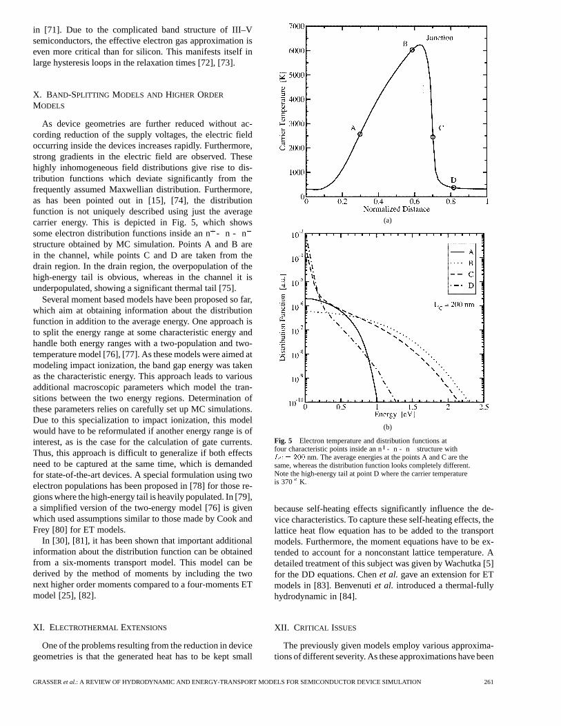
As device geometries are further reduced without ac-cording reduction of the supply voltages, the electric fieldoccurring inside the devices increases rapidly. Furthermore,strong gradients in the electric field are observed. Thesehighly inhomogeneous field distributions give rise to dis-tribution functions which deviate significantly from thefrequently assumed Maxwellian distribution. Furthermore,as has been pointed out in [15], [74], the distributionfunction is not uniquely described using just the averagecarrier energy. This is depicted in Fig. 5, which showssome electron distribution functions inside an n- n - nstructure obtained by MC simulation. Points A and B arein the channel, while points C and D are taken from thedrain region. In the drain region, the overpopulation of thehigh-energy tail is obvious, whereas in the channel it isunderpopulated, showing a significant thermal tail [75].

Several moment based models have been proposed so far,which aim at obtaining information about the distributionfunction in addition to the average energy. One approach isto split the energy range at some characteristic energy andhandle both energy ranges with a two-population and two-temperature model [76], [77]. As these models were aimed atmodeling impact ionization, the band gap energy was takenas the characteristic energy. This approach leads to variousadditional macroscopic parameters which model the tran-sitions between the two energy regions. Determination ofthese parameters relies on carefully set up MC simulations.Due to this specialization to impact ionization, this modelwould have to be reformulated if another energy range is ofinterest, as is the case for the calculation of gate currents.Thus, this approach is difficult to generalize if both effectsneed to be captured at the same time, which is demandedfor state-of-the-art devices. A special formulation using twoelectron populations has been proposed in [78] for those re-gions where the high-energy tail is heavily populated. In [79],a simplified version of the two-energy model [76] is givenwhich used assumptions similar to those made by Cook andFrey [80] for ET models.

In [30], [81], it has been shown that important additionalinformation about the distribution function can be obtainedfrom a six-moments transport model. This model can bederived by the method of moments by including the twonext higher order moments compared to a four-moments ETmodel [25], [82].

XI. ELECTROTHERMAL EXTENSIONS

One of the problems resulting from the reduction in devicegeometries is that the generated heat has to be kept small

(a)

(b)

Fig. 5 Electron temperature and distribution functions atfour characteristic points inside an n- n - n structure withLc = 200 nm. The average energies at the points A and C are thesame, whereas the distribution function looks completely different.Note the high-energy tail at point D where the carrier temperatureis 370� K.

because self-heating effects significantly influence the de-vice characteristics. To capture these self-heating effects, thelattice heat flow equation has to be added to the transportmodels. Furthermore, the moment equations have to be ex-tended to account for a nonconstant lattice temperature. Adetailed treatment of this subject was given by Wachutka [5]for the DD equations. Chenet al. gave an extension for ETmodels in [83]. Benvenutiet al. introduced a thermal-fullyhydrodynamic in [84].

XII. CRITICAL ISSUES

The previously given models employ various approxima-tions of different severity. As these approximations have been


discussed extensively in the literature, they will be summa-rized in this section.

A. Closure

The method of moments transforms the BTE into an equiv-alent, infinite set of equations. A severe approximation is thetruncation to a finite number of equations (normally three orfour). The equation of highest order contains the moment ofthe next order, which has to be suitably approximated usingavailable information, typically the lower order moments.Even though no form of the distribution function needs to beassumed in the derivation, an implicit coupling of the highestorder moment and the lower order moments is enforced bythis closure. Furthermore, the method of moments deliversmore unknowns than equations which have to be eliminatedby separate closure relations.

One approach to derive a suitable closure relation is toassume a distribution function and calculate the fourth-ordermoment. Geurts [85] expanded the distribution functionaround a drifted and heated Maxwellian distribution usingHermite polynomials. This gives a closure relation whichgeneralizes the standard Maxwellian closure. However,these closures proved to be numerically unstable for strongelectric fields. Liotta and Struchtrup [32] investigated aclosure using an equilibrium Maxwellian, which provedto be numerically very efficient but with unacceptableerrors for strong electric fields. For a discussion on heatedFermi–Dirac distributions see [19], [57]. Different closurerelations available in the literature are compared in [38].

By introducing a non-Maxwellian and nonparabolicitycorrection factor

(92)

in the closure for the highest order moment

(93)

we obtain the following expression for the energy flux:

(94)

(95)

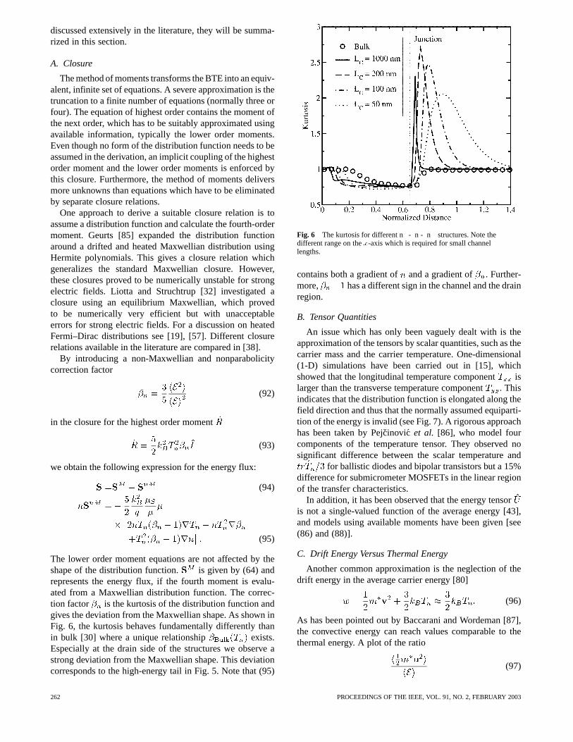
The lower order moment equations are not affected by theshape of the distribution function. is given by (64) andrepresents the energy flux, if the fourth moment is evalu-ated from a Maxwellian distribution function. The correc-tion factor is the kurtosis of the distribution function andgives the deviation from the Maxwellian shape. As shown inFig. 6, the kurtosis behaves fundamentally differently thanin bulk [30] where a unique relationship exists.Especially at the drain side of the structures we observe astrong deviation from the Maxwellian shape. This deviationcorresponds to the high-energy tail in Fig. 5. Note that (95)

Fig. 6 The kurtosis for different n- n - n structures. Note thedifferent range on thex-axis which is required for small channellengths.

contains both a gradient of and a gradient of . Further-more, has a different sign in the channel and the drainregion.

B. Tensor Quantities

An issue which has only been vaguely dealt with is theapproximation of the tensors by scalar quantities, such as thecarrier mass and the carrier temperature. One-dimensional(1-D) simulations have been carried out in [15], whichshowed that the longitudinal temperature componentislarger than the transverse temperature component. Thisindicates that the distribution function is elongated along thefield direction and thus that the normally assumed equiparti-tion of the energy is invalid (see Fig. 7). A rigorous approachhas been taken by Pejcinovic et al. [86], who model fourcomponents of the temperature tensor. They observed nosignificant difference between the scalar temperature and

for ballistic diodes and bipolar transistors but a 15%difference for submicrometer MOSFETs in the linear regionof the transfer characteristics.

In addition, it has been observed that the energy tensoris not a single-valued function of the average energy [43],and models using available moments have been given [see(86) and (88)].

C. Drift Energy Versus Thermal Energy

Another common approximation is the neglection of thedrift energy in the average carrier energy [80]

(96)

As has been pointed out by Baccarani and Wordeman [87],the convective energy can reach values comparable to thethermal energy. A plot of the ratio

(97)


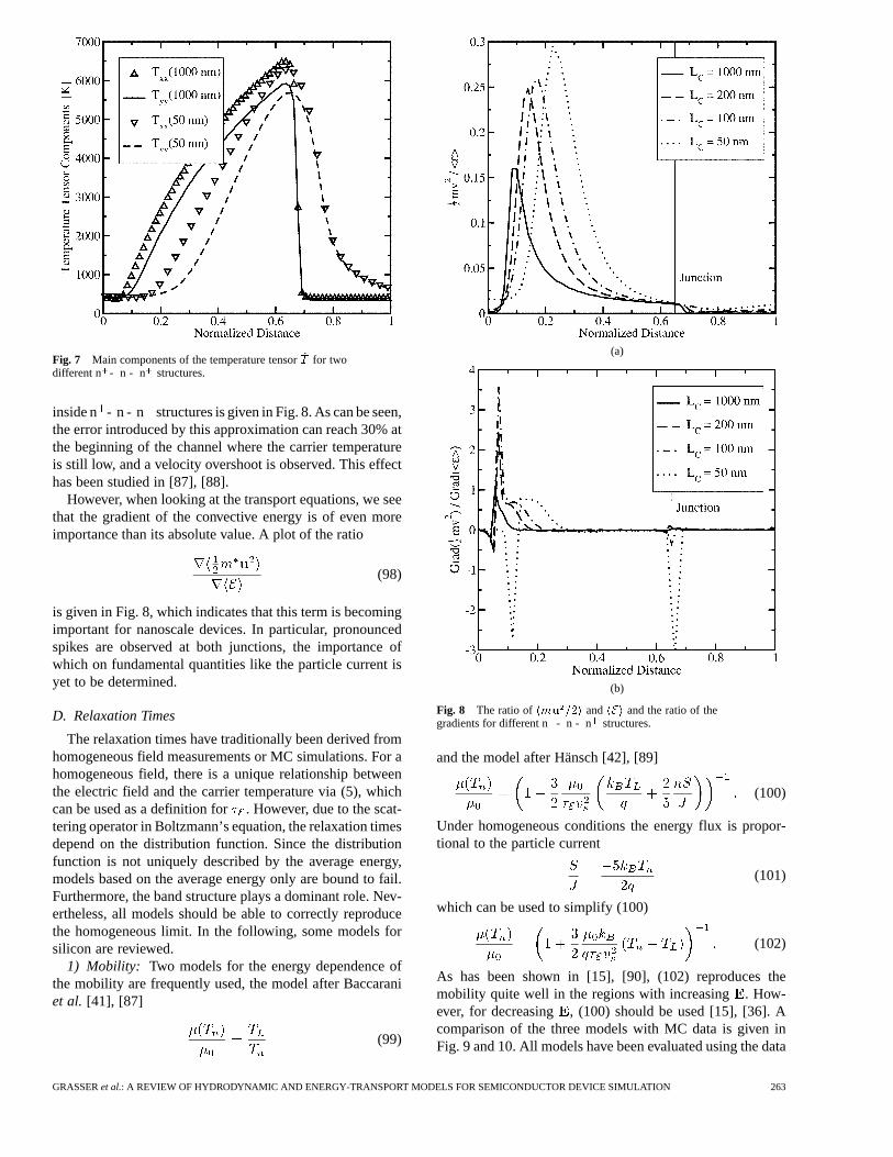
Fig. 7 Main components of the temperature tensorT for twodifferent n - n - n structures.

inside n - n - n structures is given in Fig. 8. As can be seen,the error introduced by this approximation can reach 30% atthe beginning of the channel where the carrier temperatureis still low, and a velocity overshoot is observed. This effecthas been studied in [87], [88].

However, when looking at the transport equations, we seethat the gradient of the convective energy is of even moreimportance than its absolute value. A plot of the ratio

(98)

is given in Fig. 8, which indicates that this term is becomingimportant for nanoscale devices. In particular, pronouncedspikes are observed at both junctions, the importance ofwhich on fundamental quantities like the particle current isyet to be determined.

D. Relaxation Times

The relaxation times have traditionally been derived fromhomogeneous field measurements or MC simulations. For ahomogeneous field, there is a unique relationship betweenthe electric field and the carrier temperature via (5), whichcan be used as a definition for. However, due to the scat-tering operator in Boltzmann’s equation, the relaxation timesdepend on the distribution function. Since the distributionfunction is not uniquely described by the average energy,models based on the average energy only are bound to fail.Furthermore, the band structure plays a dominant role. Nev-ertheless, all models should be able to correctly reproducethe homogeneous limit. In the following, some models forsilicon are reviewed.

1) Mobility: Two models for the energy dependence ofthe mobility are frequently used, the model after Baccaraniet al. [41], [87]

(99)

(a)

(b)

Fig. 8 The ratio ofhmu =2i andhEi and the ratio of thegradients for different n- n - n structures.

and the model after Hänsch [42], [89]

(100)

Under homogeneous conditions the energy flux is propor-tional to the particle current

(101)

which can be used to simplify (100)

(102)

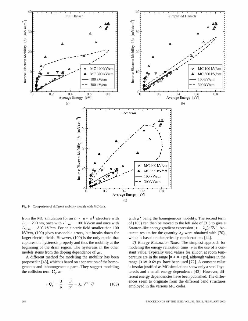
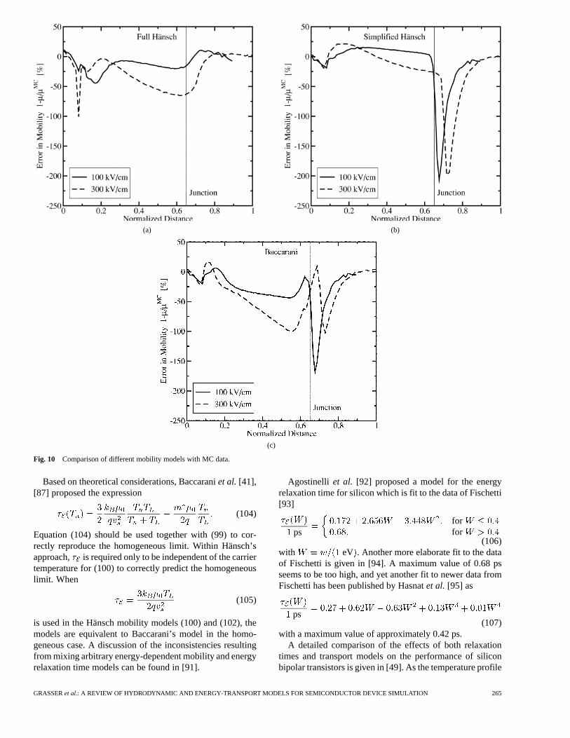
As has been shown in [15], [90], (102) reproduces themobility quite well in the regions with increasing. How-ever, for decreasing , (100) should be used [15], [36]. Acomparison of the three models with MC data is given inFig. 9 and 10. All models have been evaluated using the data


(a) (b)

(c)

Fig. 9 Comparison of different mobility models with MC data.

from the MC simulation for an n- n - n structure withnm, once with kV/cm and once with

kV/cm. For an electric field smaller than 100kV/cm, (100) gives reasonable errors, but breaks down forlarger electric fields. However, (100) is the only model thatcaptures the hysteresis properly and thus the mobility at thebeginning of the drain region. The hysteresis in the othermodels stems from the doping dependence of.

A different method for modeling the mobility has beenproposed in [43], which is based on a separation of the homo-geneous and inhomogeneous parts. They suggest modelingthe collision term as

(103)

with being the homogeneous mobility. The second termof (103) can then be moved to the left side of (31) to give aStratton-like energy gradient expression . Ac-curate results for the quantity were obtained with (70),which is based on theoretically considerations [44].

2) Energy Relaxation Time:The simplest approach formodeling the energy relaxation time is the use of a con-stant value. Typically used values for silicon at room tem-perature are in the range ps, although values in therange ps have been used [72]. A constant valueis insofar justified as MC simulations show only a small hys-teresis and a small energy dependence [43]. However, dif-ferent energy dependencies have been published. The differ-ences seem to originate from the different band structuresemployed in the various MC codes.


(a) (b)

(c)

Fig. 10 Comparison of different mobility models with MC data.

Based on theoretical considerations, Baccaraniet al. [41],[87] proposed the expression

(104)

Equation (104) should be used together with (99) to cor-rectly reproduce the homogeneous limit. Within Hänsch’sapproach, is required only to be independent of the carriertemperature for (100) to correctly predict the homogeneouslimit. When

(105)

is used in the Hänsch mobility models (100) and (102), themodels are equivalent to Baccarani’s model in the homo-geneous case. A discussion of the inconsistencies resultingfrom mixing arbitrary energy-dependent mobility and energyrelaxation time models can be found in [91].

Agostinelli et al. [92] proposed a model for the energyrelaxation time for silicon which is fit to the data of Fischetti[93]

psforfor

(106)with eV . Another more elaborate fit to the dataof Fischetti is given in [94]. A maximum value of 0.68 psseems to be too high, and yet another fit to newer data fromFischetti has been published by Hasnatet al. [95] as

ps(107)

with a maximum value of approximately 0.42 ps.A detailed comparison of the effects of both relaxation

times and transport models on the performance of siliconbipolar transistors is given in [49]. As the temperature profile


occurring inside the device is very sensitive to, this dis-agreement is rather unsatisfactory, although we believe forbulk silicon it should be in the range ps .

3) Energy Flux Mobility: The ratio of the energy fluxmobility and the mobility is usually modeled as a con-stant with values in the range (see, for instance,[15], [43]). In [43], it is proposed to model as

(108)

which is in analogy to (103). Here, is the homogeneousenergy flux mobility. Expressions for and can befound in [43].

E. Spurious Velocity Overshoot

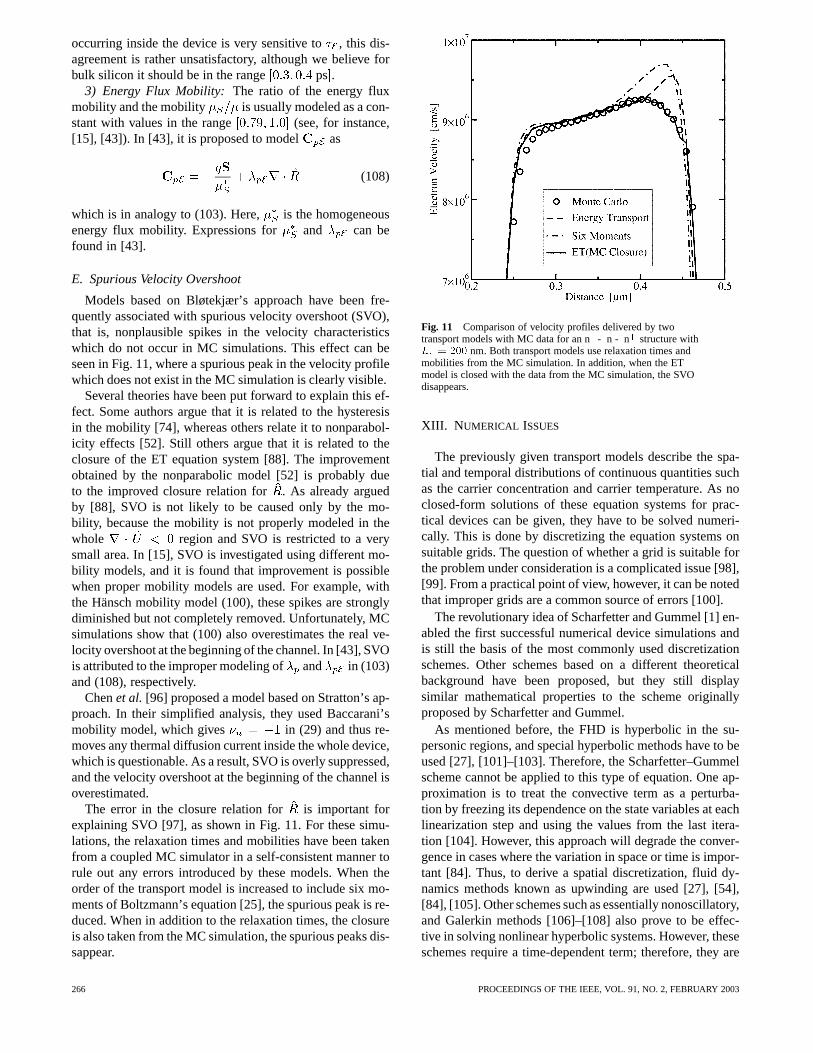
Models based on Bløtekjær’s approach have been fre-quently associated with spurious velocity overshoot (SVO),that is, nonplausible spikes in the velocity characteristicswhich do not occur in MC simulations. This effect can beseen in Fig. 11, where a spurious peak in the velocity profilewhich does not exist in the MC simulation is clearly visible.

Several theories have been put forward to explain this ef-fect. Some authors argue that it is related to the hysteresisin the mobility [74], whereas others relate it to nonparabol-icity effects [52]. Still others argue that it is related to theclosure of the ET equation system [88]. The improvementobtained by the nonparabolic model [52] is probably dueto the improved closure relation for. As already arguedby [88], SVO is not likely to be caused only by the mo-bility, because the mobility is not properly modeled in thewhole region and SVO is restricted to a verysmall area. In [15], SVO is investigated using different mo-bility models, and it is found that improvement is possiblewhen proper mobility models are used. For example, withthe Hänsch mobility model (100), these spikes are stronglydiminished but not completely removed. Unfortunately, MCsimulations show that (100) also overestimates the real ve-locity overshoot at the beginning of the channel. In [43], SVOis attributed to the improper modeling of and in (103)and (108), respectively.

Chenet al. [96] proposed a model based on Stratton’s ap-proach. In their simplified analysis, they used Baccarani’smobility model, which gives in (29) and thus re-moves any thermal diffusion current inside the whole device,which is questionable. As a result, SVO is overly suppressed,and the velocity overshoot at the beginning of the channel isoverestimated.

The error in the closure relation for is important forexplaining SVO [97], as shown in Fig. 11. For these simu-lations, the relaxation times and mobilities have been takenfrom a coupled MC simulator in a self-consistent manner torule out any errors introduced by these models. When theorder of the transport model is increased to include six mo-ments of Boltzmann’s equation [25], the spurious peak is re-duced. When in addition to the relaxation times, the closureis also taken from the MC simulation, the spurious peaks dis-sappear.

Fig. 11 Comparison of velocity profiles delivered by twotransport models with MC data for an n- n - n structure withL = 200 nm. Both transport models use relaxation times andmobilities from the MC simulation. In addition, when the ETmodel is closed with the data from the MC simulation, the SVOdisappears.

XIII. N UMERICAL ISSUES

The previously given transport models describe the spa-tial and temporal distributions of continuous quantities suchas the carrier concentration and carrier temperature. As noclosed-form solutions of these equation systems for prac-tical devices can be given, they have to be solved numeri-cally. This is done by discretizing the equation systems onsuitable grids. The question of whether a grid is suitable forthe problem under consideration is a complicated issue [98],[99]. From a practical point of view, however, it can be notedthat improper grids are a common source of errors [100].

The revolutionary idea of Scharfetter and Gummel [1] en-abled the first successful numerical device simulations andis still the basis of the most commonly used discretizationschemes. Other schemes based on a different theoreticalbackground have been proposed, but they still displaysimilar mathematical properties to the scheme originallyproposed by Scharfetter and Gummel.

As mentioned before, the FHD is hyperbolic in the su-personic regions, and special hyperbolic methods have to beused [27], [101]–[103]. Therefore, the Scharfetter–Gummelscheme cannot be applied to this type of equation. One ap-proximation is to treat the convective term as a perturba-tion by freezing its dependence on the state variables at eachlinearization step and using the values from the last itera-tion [104]. However, this approach will degrade the conver-gence in cases where the variation in space or time is impor-tant [84]. Thus, to derive a spatial discretization, fluid dy-namics methods known as upwinding are used [27], [54],[84], [105]. Other schemes such as essentially nonoscillatory,and Galerkin methods [106]–[108] also prove to be effec-tive in solving nonlinear hyperbolic systems. However, theseschemes require a time-dependent term; therefore, they are


less efficient when applied to steady-state problems. Further-more, when the convective terms are involved, the handlingof boundary conditions becomes more difficult [103], [109],[110].

When the convective terms are neglected, Schar-fetter–Gummel-type schemes can be applied to higherorder transport models. However, as this extension of theScharfetter–Gummel scheme is not straightforward, severalvariants exist [111]–[116]. In general it can be noted thatthe convergence properties degrade significantly whencompared to the classic DD model. Some improvement hasbeen obtained by refining the discretization scheme [114],but the problem still persists. Other improvements in termsof convergence are based on iteration schemes where theequations are solve in a decoupled manner [8], [117], similarto an idea of Gummel for the DD model [118].

XIV. V ALIDITY OF MOMENT-BASED MODELS

When the critical dimensions of devices shrink below acertain value (around 200 nm for silicon at room tempera-ture) MC simulations reveal strong off-equilibrium transporteffects such as velocity overshoot and nonlocality of impor-tant model parameters. Therefore, the range of validity formoment-based models has been extensively examined. Fur-thermore, with shrinking device geometries, quantum effectsgain more importance and limit the validity for the BTE it-self [119]. Banoo and Lundstrom [120] compared the resultsobtained by (56)–(59) with a DD model and a solution of theBTE obtained by using the scattering matrix approach. Theyfound that this ET model dramatically overestimates both thedrain current and the velocity inside the device. Tomizawaetal. [121] found through a comparison with MC simulationsthat relaxation time based models tend to overestimate non-stationary carrier dynamics, especially the energy distribu-tion. Nekoveeet al. [31] compared moment hierarchy basedmodels with a solution of the BTE and found that their modelfails in the prediction of ballistic diodes because the equationhierarchy converges too slowly. However, their “moment”model was based on an Ansatz for the distribution functionusing a Maxwellian shape multiplied by a sum of Hermitepolynomials. Indeed, such an expansion of the distributionfunction converges too slowly [30], but as there the parame-ters of the distribution function and not the moments of theBTE are considered, we do not feel their conclusions areequally valid for moment-based models. A conclusion sim-ilar to Nekovee’s was drawn by Liotta and Struchtrup [32],who found that a hierarchy containing 12 moment equationswas needed to reproduce results similar to those obtained byspherical harmonics expansions. In their model, the closurerelations were calculated via an Ansatz for the distributionfunction; therefore, they cannot easily be generalized to mo-ment-based models with carefully derived closure relations.

The nonequilibrium transport in nanoscale devices is char-acterized by the ratio , where is the inelastic meanfree path and is the device characteristic length. Assuming

where and taking the en-ergy relaxation time to be 0.3 ps for silicon, we have

. This gives – nm dependingon the electron temperature. It takes a distance of at least

for electrons to attain a “local equilibrium” average en-ergy. Thus, for any device with less than 200 nm, the car-rier transport in the channel is intrinsically nonstationary. For

– nm, this ratio becomes smaller than one. Thisimplies that in this quasiballistic regime, even if only 50%of the transport is ballistic, it is rather difficult to constructa “universal” hydrodynamic model because the model nowdepends on this ratio. In fact, our own simulations show thatin the modeling of , the plot of versus is al-most a single-valued function of , e.g., . For

nm, is almost linear with a slope of 1.6/3. Fornm, is a straight line with a slope of 3/5.

For nm, is also a straight line but with a slopeof 2/3. This implies that if we want to model in this regime,we have approximately , where is a func-tion of . Therefore, when considering devices in thenanometer regime, it might be wise to compare the solutionof moment-based models to a solution of Boltzmann’s equa-tion obtained by either MC or other methods.

XV. SIMPLIFIED MODELS

Despite the limitations and approximations contained inthe moment equations given previously, the handling of theseequations is still far more complicated than that of the robustand well-studied DD equations. Thus, several researchershave tried to find suitable approximations to simplify theproblem. These approximations were frequently used inpostprocessors to account for an average energy distributiondifferent from the local approximation. Slotboomet al.[122] used this technique to calculate energy-dependentimpact ionization rates via a postprocessing model. Cookand Frey [80], [123] proposed a simplified model by usingthe approximations and in a two-dimen-sional (2-D) silicon MESFET to yield

(109)Thus, the energy balance equation and the continuity equa-tion become decoupled, and the complexity of the problemis considerably reduced. Approximations for GaAs werealso given. Although these approximations might havedelivered promising results, progress in the size reduction ofstate-of-the-art devices makes the assumptions and

questionable. In particular, for deep-submicrom-eter MOSFETs, velocity overshoot influences the electricfield distribution for a given bias condition and effectivelydefines a higher drain saturation voltage, which in turndefines a higher current [124].

To bring the ET equations into a self-adjoint form, Linetal. [125] approximated the carrier temperature in the diffu-sion coefficient by the lattice temperature as

(110)


which will underestimate the diffusion current by a factor of– for today’s devices; therefore, this technique cannot

be recommended.Another simplified model is Thornber’s generalized cur-

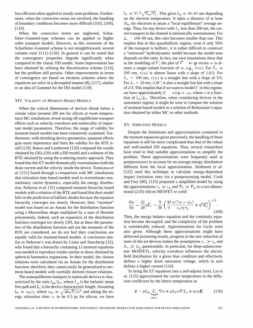
rent equation [126], later called the augmented DD model[127], [128]. In these models, the field dependence of thetransport coefficients is extended to include the gradient ofthe electric field. The motivation for this model is very sim-ilar to (109). However, the augmented DD model incorpo-rates nonlocality effects using the electric field rather thanthe average energy. It can successfully catch nonlocal effectsoccurring in the device when the electric field is rising, butfails to do so when the electric field is abruptly decreasing,such as near the drain region in MOSFETs. Because of this,its usefulness in nanoscale device simulation is very limited.

XVI. A PPLICATION TO MOS TRANSISTORS

So far, the transport models have been checked with n-n-n structures. Due to their simplicity, these are the mostcommonly used structures when a comparison with MC datais required. This is mainly because they are 1-D and requireonly one carrier type. Therefore, the influence of the variousparameters on basic quantities like the velocity or the carriertemperature can be more easily separated and interpreted.As can be seen from the previous examples, even for thesesimple structures, such an interpretation is far from trivial.

Although it has been frequently claimed that n-n-nstructures emulate the behavior of MOS transistors, themost important devices in silicon technology, this is onlypartly true. MOS transistors are inherently 2-D devices,a fact that makes a comparison of moment-based modelswith MC more involved. In the following, the most impor-tant differences to n-n-n structures are compared. TheMC simulations were performed using MINIMOS [129],whereas MINIMOS-NT [130] was used for the ET model,which is based on (56)–(58) and (64). Hänsch’s mobilitymodel (102), a ratio of 0.8, and ps havebeen chosen because this is basically the model available incommercial simulators. No fitting was performed.

The basic quantities velocity and temperature show similarfeatures for MOS transistors as shown in Fig. 12 and for n-n-n structures (cf. Fig. 1). However, the velocity overshoot atthe beginning of the channel and the SVO observed in n-n-n structures coincide in MOS transistors to give a singleovershoot in the pinch-off region.

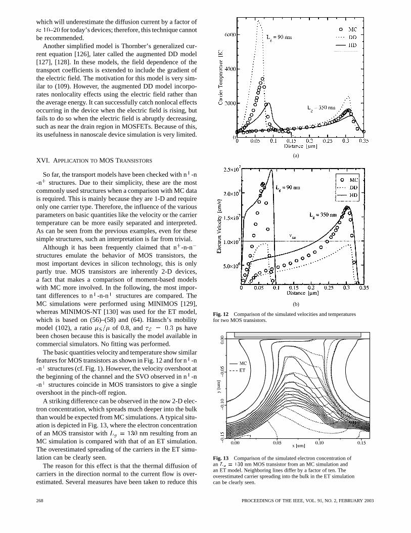
A striking difference can be observed in the now 2-D elec-tron concentration, which spreads much deeper into the bulkthan would be expected from MC simulations. A typical situ-ation is depicted in Fig. 13, where the electron concentrationof an MOS transistor with nm resulting from anMC simulation is compared with that of an ET simulation.The overestimated spreading of the carriers in the ET simu-lation can be clearly seen.

The reason for this effect is that the thermal diffusion ofcarriers in the direction normal to the current flow is over-estimated. Several measures have been taken to reduce this

(a)

(b)

Fig. 12 Comparison of the simulated velocities and temperaturesfor two MOS transistors.

Fig. 13 Comparison of the simulated electron concentration ofanL = 130 nm MOS transistor from an MC simulation andan ET model. Neighboring lines differ by a factor of ten. Theoverestimated carrier spreading into the bulk in the ET simulationcan be clearly seen.


(a)

(b)

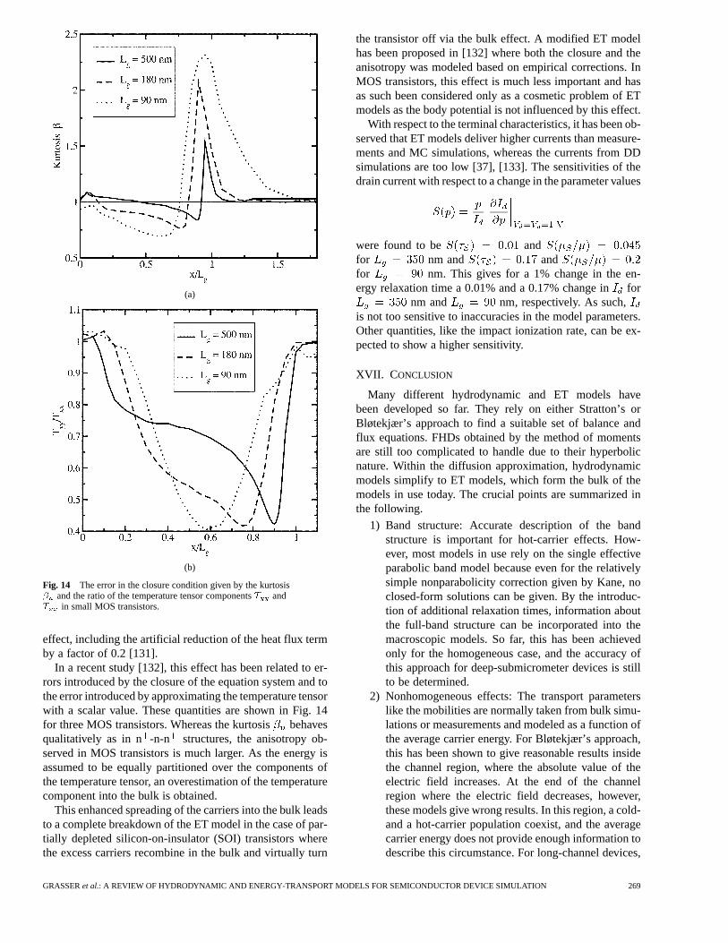
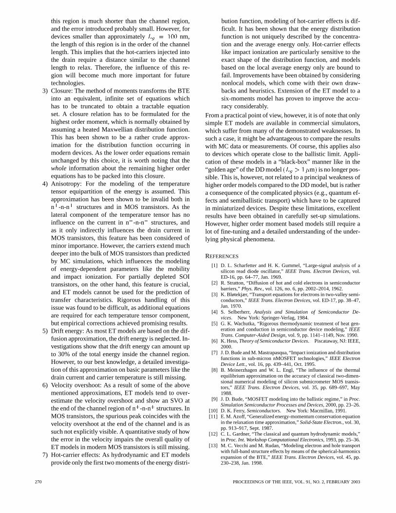
Fig. 14 The error in the closure condition given by the kurtosis� and the ratio of the temperature tensor componentsT andT in small MOS transistors.

effect, including the artificial reduction of the heat flux termby a factor of 0.2 [131].

In a recent study [132], this effect has been related to er-rors introduced by the closure of the equation system and tothe error introduced by approximating the temperature tensorwith a scalar value. These quantities are shown in Fig. 14for three MOS transistors. Whereas the kurtosisbehavesqualitatively as in n -n-n structures, the anisotropy ob-served in MOS transistors is much larger. As the energy isassumed to be equally partitioned over the components ofthe temperature tensor, an overestimation of the temperaturecomponent into the bulk is obtained.

This enhanced spreading of the carriers into the bulk leadsto a complete breakdown of the ET model in the case of par-tially depleted silicon-on-insulator (SOI) transistors wherethe excess carriers recombine in the bulk and virtually turn

the transistor off via the bulk effect. A modified ET modelhas been proposed in [132] where both the closure and theanisotropy was modeled based on empirical corrections. InMOS transistors, this effect is much less important and hasas such been considered only as a cosmetic problem of ETmodels as the body potential is not influenced by this effect.

With respect to the terminal characteristics, it has been ob-served that ET models deliver higher currents than measure-ments and MC simulations, whereas the currents from DDsimulations are too low [37], [133]. The sensitivities of thedrain current with respect to a change in the parameter values

were found to be andfor nm and andfor nm. This gives for a 1% change in the en-ergy relaxation time a 0.01% and a 0.17% change infor

nm and nm, respectively. As such,is not too sensitive to inaccuracies in the model parameters.Other quantities, like the impact ionization rate, can be ex-pected to show a higher sensitivity.

XVII. C ONCLUSION

Many different hydrodynamic and ET models havebeen developed so far. They rely on either Stratton’s orBløtekjær’s approach to find a suitable set of balance andflux equations. FHDs obtained by the method of momentsare still too complicated to handle due to their hyperbolicnature. Within the diffusion approximation, hydrodynamicmodels simplify to ET models, which form the bulk of themodels in use today. The crucial points are summarized inthe following.

1) Band structure: Accurate description of the bandstructure is important for hot-carrier effects. How-ever, most models in use rely on the single effectiveparabolic band model because even for the relativelysimple nonparabolicity correction given by Kane, noclosed-form solutions can be given. By the introduc-tion of additional relaxation times, information aboutthe full-band structure can be incorporated into themacroscopic models. So far, this has been achievedonly for the homogeneous case, and the accuracy ofthis approach for deep-submicrometer devices is stillto be determined.

2) Nonhomogeneous effects: The transport parameterslike the mobilities are normally taken from bulk simu-lations or measurements and modeled as a function ofthe average carrier energy. For Bløtekjær’s approach,this has been shown to give reasonable results insidethe channel region, where the absolute value of theelectric field increases. At the end of the channelregion where the electric field decreases, however,these models give wrong results. In this region, a cold-and a hot-carrier population coexist, and the averagecarrier energy does not provide enough information todescribe this circumstance. For long-channel devices,


this region is much shorter than the channel region,and the error introduced probably small. However, fordevices smaller than approximately nm,the length of this region is in the order of the channellength. This implies that the hot-carriers injected intothe drain require a distance similar to the channellength to relax. Therefore, the influence of this re-gion will become much more important for futuretechnologies.

3) Closure: The method of moments transforms the BTEinto an equivalent, infinite set of equations whichhas to be truncated to obtain a tractable equationset. A closure relation has to be formulated for thehighest order moment, which is normally obtained byassuming a heated Maxwellian distribution function.This has been shown to be a rather crude approx-imation for the distribution function occurring inmodern devices. As the lower order equations remainunchanged by this choice, it is worth noting that thewhole information about the remaining higher orderequations has to be packed into this closure.

4) Anisotropy: For the modeling of the temperaturetensor equipartition of the energy is assumed. Thisapproximation has been shown to be invalid both inn -n-n structures and in MOS transistors. As thelateral component of the temperature tensor has noinfluence on the current in n-n-n structures, andas it only indirectly influences the drain current inMOS transistors, this feature has been considered ofminor importance. However, the carriers extend muchdeeper into the bulk of MOS transistors than predictedby MC simulations, which influences the modelingof energy-dependent parameters like the mobilityand impact ionization. For partially depleted SOItransistors, on the other hand, this feature is crucial,and ET models cannot be used for the prediction oftransfer characteristics. Rigorous handling of thisissue was found to be difficult, as additional equationsare required for each temperature tensor component,but empirical corrections achieved promising results.

5) Drift energy: As most ET models are based on the dif-fusion approximation, the drift energy is neglected. In-vestigations show that the drift energy can amount upto 30% of the total energy inside the channel region.However, to our best knowledge, a detailed investiga-tion of this approximation on basic parameters like thedrain current and carrier temperature is still missing.

6) Velocity overshoot: As a result of some of the abovementioned approximations, ET models tend to over-estimate the velocity overshoot and show an SVO atthe end of the channel region of n-n-n structures. InMOS transistors, the spurious peak coincides with thevelocity overshoot at the end of the channel and is assuch not explicitly visible. A quantitative study of howthe error in the velocity impairs the overall quality ofET models in modern MOS transistors is still missing.

7) Hot-carrier effects: As hydrodynamic and ET modelsprovide only the first two moments of the energy distri-

bution function, modeling of hot-carrier effects is dif-ficult. It has been shown that the energy distributionfunction is not uniquely described by the concentra-tion and the average energy only. Hot-carrier effectslike impact ionization are particularly sensitive to theexact shape of the distribution function, and modelsbased on the local average energy only are bound tofail. Improvements have been obtained by consideringnonlocal models, which come with their own draw-backs and heuristics. Extension of the ET model to asix-moments model has proven to improve the accu-racy considerably.

From a practical point of view, however, it is of note that onlysimple ET models are available in commercial simulators,which suffer from many of the demonstrated weaknesses. Insuch a case, it might be advantageous to compare the resultswith MC data or measurements. Of course, this applies alsoto devices which operate close to the ballistic limit. Appli-cation of these models in a “black-box” manner like in the“golden age” of the DD model m is no longer pos-sible. This is, however, not related to a principal weakness ofhigher order models compared to the DD model, but is rathera consequence of the complicated physics (e.g., quantum ef-fects and semiballistic transport) which have to be capturedin miniaturized devices. Despite these limitations, excellentresults have been obtained in carefully set-up simulations.However, higher order moment based models still require alot of fine-tuning and a detailed understanding of the under-lying physical phenomena.

REFERENCES

[1] D. L. Scharfetter and H. K. Gummel, “Large-signal analysis of asilicon read diode oscillator,”IEEE Trans. Electron Devices, vol.ED-16, pp. 64–77, Jan. 1969.

[2] R. Stratton, “Diffusion of hot and cold electrons in semiconductorbarriers,”Phys. Rev., vol. 126, no. 6, pp. 2002–2014, 1962.

[3] K. Bløtekjær, “Transport equations for electrons in two-valley semi-conductors,”IEEE Trans. Electron Devices, vol. ED-17, pp. 38–47,Jan. 1970.

[4] S. Selberherr,Analysis and Simulation of Semiconductor De-vices. New York: Springer-Verlag, 1984.

[5] G. K. Wachutka, “Rigorous thermodynamic treatment of heat gen-eration and conduction in semiconductor device modeling,”IEEETrans. Computer-Aided Design, vol. 9, pp. 1141–1149, Nov. 1990.

[6] K. Hess,Theory of Semiconductor Devices. Piscataway, NJ: IEEE,2000.

[7] J. D. Bude and M. Mastrapasqua, “Impact ionization and distributionfunctions in sub-micron nMOSFET technologies,”IEEE ElectronDevice Lett., vol. 16, pp. 439–441, Oct. 1995.

[8] B. Meinerzhagen and W. L. Engl, “The influence of the thermalequilibrium approximation on the accuracy of classical two-dimen-sional numerical modeling of silicon submicrometer MOS transis-tors,” IEEE Trans. Electron Devices, vol. 35, pp. 689–697, May1988.

[9] J. D. Bude, “MOSFET modeling into the ballistic regime,” inProc.Simulation Semiconductor Processes and Devices, 2000, pp. 23–26.

[10] D. K. Ferry,Semiconductors. New York: Macmillan, 1991.[11] E. M. Azoff, “Generalized energy-momentum conservation equation

in the relaxation time approximation,”Solid-State Electron., vol. 30,pp. 913–917, Sept. 1987.

[12] C. L. Gardner, “The classical and quantum hydrodynamic models,”in Proc. Int. Workshop Computational Electronics, 1993, pp. 25–36.

[13] M. C. Vecchi and M. Rudan, “Modeling electron and hole transportwith full-band structure effects by means of the spherical-harmonicsexpansion of the BTE,”IEEE Trans. Electron Devices, vol. 45, pp.230–238, Jan. 1998.


[14] C.-K. Lin, N. Goldsman, I. Mayergoyz, S. Aronowitz, and N. Belova,“Advances in spherical harmonic device modeling: Calibration andnanoscale electron dynamics,” inProc. Simulation SemiconductorProcesses and Devices, 1999, pp. 167–170.

[15] S.-C. Lee and T.-W. Tang, “Transport coefficients for a silicon hy-drodynamic model extracted from inhomogeneous monte-carlo cal-culations,”Solid-State Electron., vol. 35, no. 4, pp. 561–569, 1992.

[16] R. Thoma, A. Emunds, B. Meinerzhagen, H. J. Peifer, and W.L. Engl, “Hydrodynamic equations for semiconductors with non-parabolic band structure,”IEEE Trans. Electron Devices, vol. 38,pp. 1343–1353, June 1991.

[17] E. O. Kane, “Band structure of indium antimonide,”J. Phys. Chem.Solids, vol. 1, pp. 249–261, 1957.

[18] D. Cassi and B. Riccò, “An analytical model of the energy distri-bution of hot electrons,”IEEE Trans. Electron Devices, vol. 37, pp.1514–1521, June 1990.

[19] A. W. Smith and K. F. Brennan, “Non-parabolic hydrodynamic for-mulations for the simulation of inhomogeneous semiconductor de-vices,”Solid-State Electron., vol. 39, no. 11, pp. 1659–1668, 1996.

[20] M. V. Fischetti and S. E. Laux, “Monte Carlo analysis of electrontransport in small semiconductor devices including band-structureand space-charge effects,”Phys. Rev. B, vol. 38, no. 14, pp.9721–9745, 1988.

[21] Y. Apanovich, E. Lyumkis, B. Polsky, A. Shur, and P. Blakey,“Steady-state and transient analysis of submicron devices usingenergy balance and simplified hydrodynamic models,”IEEE Trans.Computer-Aided Design, vol. 13, pp. 702–711, June 1994.

[22] K. Hess,Advanced Theory of Semiconductor Devices. EnglewoodCliffs, NJ: Prentice-Hall, 1988.

[23] E. M. Azoff, “Energy transport numerical simulation of graded Al-GaAs/GaAs heterojunction bipolar transistors,”IEEE Trans. Elec-tron Devices, vol. 36, pp. 609–616, Apr. 1989.

[24] M. Lundstrom,Fundamentals of Carrier Transport. Reading, MA:Addison-Wesley, 1990, vol. 10, Modular Series on Solid State De-vices.

[25] T. Grasser, H. Kosina, M. Gritsch, and S. Selberherr, “Using six mo-ments of Boltzmann’s transport equation for device simulation,”J.Appl. Phys., vol. 90, no. 5, pp. 2389–2396, 2001.

[26] K. Souissi, F. Odeh, H. H. K. Tang, and A. Gnudi, “Comparativestudies of hydrodynamic and energy transport models,”COMPEL,vol. 13, no. 2, pp. 439–453, 1994.

[27] C. L. Gardner, “Numerical simulation of a steady-state electronshock wave in a submicrometer semiconductor device,”IEEETrans. Electron Devices, vol. 38, pp. 392–398, Feb. 1991.

[28] C. Ringhofer, C. Schmeiser, and A. Zwirchmayer, “Momentmethods for the semiconductor boltzmann equation in boundedposition domains,”SIAM J. Numer. Anal., vol. 39, no. 3, pp.1078–1095, 2001.

[29] H. Struchtrup, “Extended moment method for electrons in semicon-ductors,”Physica A, vol. 275, pp. 229–255, 2000.

[30] T. Grasser, H. Kosina, C. Heitzinger, and S. Selberherr, “Character-ization of the hot electron distribution function using six moments,”J. Appl. Phys., vol. 91, no. 6, pp. 3869–3879, 2002.

[31] M. Nekovee, B. J. Geurts, H. M. J. Boots, and M. F. H. Schuurmans,“Failure of extended moment equation approaches to describe bal-listic transport in submicron structures,”Phys. Rev. B, vol. 45, no.10, pp. 6643–6651, 1992.

[32] S. F. Liotta and H. Struchtrup, “Moment equations for electrons insemiconductors: Comparison of spherical harmonics and full mo-ments,”Solid-State Electron., vol. 44, pp. 95–103, 2000.

[33] R. Stratton, “Semiconductor current-flow equations (Diffusionand Degeneracy),”IEEE Trans. Electron Devices, vol. ED-19, pp.1288–1292, Dec. 1972.

[34] P. T. Landsberg and S. A. Hope, “Two formulations of semicon-ductor transport equations,”Solid-State Electron., vol. 20, pp.421–429, 1977.

[35] P. T. Landsberg, “Dgrad� or grad(D�)?,” J. Appl. Phys., vol. 56,no. 4, pp. 1119–1122, 1984.

[36] T.-W. Tang and H. Gan, “Two formulations of semiconductor trans-port equations based on spherical harmonic expansion of the boltz-mann transport equation,”IEEE Trans. Electron Devices, vol. 47,pp. 1726–1732, Sept. 2000.

[37] M. Ieong and T.-W. Tang, “Influence of hydrodynamic models onthe prediction of submicrometer device characteristics,”IEEE Trans.Electron Devices, vol. 44, pp. 2242–2251, Dec. 1997.

[38] S. Ramaswamy and T.-W. Tang, “Comparison of semiconductortransport models using a Monte Carlo consistency check,”IEEETrans. Electron Devices, vol. 41, pp. 76–83, Jan. 1994.

[39] M. C. Vecchi and L. G. Reyna, “Generalized energy transport modelsfor semiconductor device simulation,”Solid-State Electron., vol. 37,no. 10, pp. 1705–1716, 1994.

[40] H. Gan and T.-W. Tang, “A new method for extracting carrier mo-bility from Monte Carlo device simulation,”IEEE Trans. ElectronDevices, vol. 48, pp. 399–401, Feb. 2001.

[41] G. Baccarani, M. Rudan, R. Guerrieri, and P. Ciampolini, “Phys-ical models for numerical device simulation,” inProcess and DeviceModeling, W. Engl, Ed. Amsterdam, The Netherlands: North-Hol-land, 1986, vol. 1, Advances in CAD for VLSI, pp. 107–158.

[42] W. Hänsch,The Drift Diffusion Equation and Its Application inMOSFET Modeling. New York: Springer-Verlag, 1991.

[43] T.-W. Tang, S. Ramaswamy, and J. Nam, “An improved hydrody-namic transport model for silicon,”IEEE Trans. Electron Devices,vol. 40, pp. 1469–1476, Aug. 1993.

[44] T.-W. Tang, X. Wang, H. Gan, and M. K. Leong, “An analytic ex-pression of thermal diffusion coefficient for the hydrodynamic sim-ulation of semiconductor devices,”VLSI Design, vol. 13, no. 1-4, pp.131–134, 2000.

[45] S. Selberherr, “MOS device modeling at 77 K,”IEEE Trans. Elec-tron Devices, vol. 36, pp. 1464–1474, Aug. 1989.

[46] A. Leone, A. Gnudi, and G. Baccarani, “Hydrodynamic simulationof semiconductor devices operating at low temperature,”IEEETrans. Computer-Aided Design, vol. 13, pp. 1400–1408, Nov. 1994.

[47] A. H. Marshak and C. M. VanVliet, “Electrical current and carrierdensity in degenerate materials with nonuniform band structure,”Proc. IEEE, vol. 72, pp. 148–164, Feb. 1984.

[48] R. Thoma, A. Emunds, B. Meinerzhagen, H. Peifer, and W. L.Engl, “A generalized hydrodynamic model capable of incorporatingMonte Carlo results,” inProc. Int. Electron Devices Meeting, 1989,pp. 139–142.

[49] A. D. Sadovnikov and D. J. Roulston, “A study of the influenceof hydrodynamic model effects on characteristics of silicon bipolartransistors,”COMPEL, vol. 12, no. 4, pp. 245–262, 1993.

[50] C. Jungeman, B. Neinhüs, and B. Meinerzhagen, “Comparativestudy for electron transit times evaluated by DD, HD, and MCdevice simulation for a SiGe HBT,”IEEE Trans. Electron Devices,vol. 48, pp. 2216–2220, Oct. 2001.

[51] T. J. Bordelon, X.-L. Wang, C. M. Maziar, and A. F. Tasch, “Ac-counting for bandstructure effects in the hydrodynamic model: Afirst-order approach for silicon device simulation,”Solid-State Elec-tron., vol. 35, no. 2, pp. 131–139, 1992.

[52] , “An efficient nonparabolic formulation of the hydrodynamicmodel for silicon device simulation,” inProc. Int. Electron DevicesMeeting, 1990, pp. 353–356.

[53] D. Chen, E. C. Kan, U. Ravaioli, C.-W. Shu, and R. W. Dutton, “Animproved energy transport model including nonparabolicity andnonmaxwellian distribution effects,”IEEE Electron Device Lett.,vol. 13, pp. 26–28, Jan. 1992.

[54] D. Xu, T.-W. Tang, and S. S. Kucherenko, “Time-dependent solu-tion of a full hydrodynamic model including convective terms andviscous effects,”VLSI Design, vol. 6, no. 1-4, pp. 173–176, 1998.

[55] H. Gan, “Re-examination of the hot-carrier transport model usingspherical harmonic expansion of the Boltzmann transport equation,”M.S. thesis, Univ. Massachusetts Amherst, Amherst, 1999.

[56] A. W. Smith and A. Rohatgi, “Non-isothermal extension of theScharfetter-Gummel technique for hot carrier transport in het-erostructure simulations,”IEEE Trans. Computer-Aided Design,vol. 12, pp. 1515–1523, Oct. 1993.

[57] A. W. Smith and K. F. Brennan, “Comparison of nonparabolic hydro-dynamic simulations for semiconductor devices,”Solid-State Elec-tron., vol. 39, no. 7, pp. 1055–1063, 1996.

[58] A. Anile and V. Romano. (1999) Hydrodynamical modeling ofcharge carrier transport in semiconductors. Summer School onIndustrial Mathematics, IST Lisboa, Lisbon, Portugal. [Online].Available: http://www.dipmat.unict.it/~anile/preprint.html

[59] O. Muscato, “The onsager reciprocity principle as a check of con-sistency for semiconductor carrier transport models,”Physica A, vol.289, pp. 422–458, 2001.

[60] M. Trovato and L. Reggiani, “Maximum entropy principle within atotal energy scheme: Application to hot-carrier transport in semicon-ductors,”Phys. Rev. B, vol. 61, no. 24, pp. 16 667–16 681, 2000.


[61] R. Thoma and W. L. Engl, “A new approach for the derivation ofmacroscopic balance equations beyond the relaxation time approx-imation,” in Simulation of Semiconductor Devices and Processes,W. Fichtner and D. Aemmer, Eds. Konstanz, Germany: Hartung-Gorre, 1991, vol. 4, pp. 185–194.

[62] T.-W. Tang and M. K. Ieong, “Why are there so many different hy-drodynamic transport models in semiconductor device simulation?,”in Proc. 2nd NASA Device Modeling Workshop, 1997, pp. 127–136.

[63] A. H. Marshak and K. M. van Vliet, “Electrical current in solidswith position-dependent band structure,”Solid-State Electron., vol.21, pp. 417–427, 1978.

[64] E. M. Azoff, “Closed-form method for solving the steady-state gen-eralized energy-momentum conservation equations,”COMPEL, vol.6, no. 1, pp. 25–30, 1987.

[65] D. L. Woolard, R. J. Trew, and M. A. Littlejohn, “Hydrodynamichot-electron transport model with Monte Carlo–generated transportparameters,”Solid-State Electron., vol. 31, no. 3/3, pp. 571–574,1988.

[66] D. L. Woolard, H. Tian, R. J. Trew, M. A. Littlejohn, and K. W.Kim, “Hydrodynamic electron-transport model: Nonparabolic cor-rections to the streaming terms,”Phys. Rev. B, vol. 44, no. 20, pp.11 119–11 132, 1991.

[67] D. L. Woolard, H. Tian, M. A. Littlejohn, K. W. Kim, R. J. Trew, M.K. Ieong, and T.-W. Tang, “Construction of higher-moment terms inthe hydrodynamic electron-transport model,”J. Appl. Phys., vol. 74,no. 10, pp. 6197–6207, 1993.

[68] R. A. Stewart and J. N. Churchill, “A fully nonparabolic hydrody-namic model for describing hot electron transport in GaAs,”Solid-State Electron., vol. 33, no. 7, pp. 819–829, 1990.

[69] R. A. Stewart, L. Ye, and J. N. Churchill, “Improved relaxation-timeformulation of collision terms for two-band hydrodynamic models,”Solid-State Electron., vol. 32, no. 6, pp. 497–502, 1989.

[70] C. L. Wilson, “Hydrodynamic carrier transport in semiconductorswith multiple band minima,”IEEE Trans. Electron Devices, vol. 35,pp. 180–187, 1988.

[71] J. C. Cao and X. L. Lei, “Simulation of an AlGa As ballisticdiode using multivalley nonparabolic hydrodynamic balance equa-tions,” Solid-State Electron., vol. 41, no. 11, pp. 1781–1785, 1997.

[72] M.-K. Ieong, “A multi-valley hydrodynamic transport model forGaAs extracted from self-consistent Monte Carlo data,” M.S. thesis,Univ. Massachusetts Amherst, Amherst, 1993.

[73] M. Ieong and T.-W. Tang, “Transport coefficients for a GaAs hydro-dynamic model extracted from inhomogenous Monte Carlo calcula-tions,” in Proc. Int. Workshop Computational Electronics, 1993, pp.65–69.

[74] G. Wolokin and J. Frey, “Overshoot effects in the relaxation timeapproximation,” inProc. 8th Int. Conf. Numerical Analysis Semi-conductor Devices and Integrated Circuits, 1992, pp. 107–108.

[75] A. Abramo and C. Fiegna, “Electron energy distributions in siliconat low applied voltages and high electric fields,”J. Appl. Phys., vol.80, no. 2, pp. 889–893, 1996.

[76] P. G. Scrobohaci and T.-W. Tang, “Modeling of the hot electron sub-population and its application to impact ionization in submicron sil-icon devices-part I: Transport equations,”IEEE Trans. Electron De-vices, vol. 41, pp. 1197–1205, July 1994.

[77] J.-G. Ahn, C.-S. Yao, Y.-J. Park, H.-S. Min, and R. W. Dutton, “Im-pact ionization modeling using simulation of high energy tail dis-tributions,” IEEE Electron Device Lett., vol. 15, pp. 348–350, Sept.1994.

[78] T. J. Bordelon, V. M. Agostinelli, X.-L. Wang, C. M. Maziar, andA. F. Tasch, “Relaxation time approximation and mixing of hotand cold electron populations,”Electron. Lett., vol. 28, no. 12, pp.1173–1175, 1992.

[79] T.-W. Tang and J. Nam, “A simplified impact ionization model basedon the average energy of hot-electron subpopulation,”IEEE ElectronDevice Lett., vol. 19, pp. 201–203, June 1998.

[80] R. K. Cook and J. Frey, “An efficient technique for two-dimensionalsimulation of velocity overshoot effects in Si and GaAs devices,”COMPEL, vol. 1, no. 2, pp. 65–87, 1982.

[81] K. Sonoda, S. T. Dunham, M. Yamaji, K. Taniguchi, and C. Ham-aguchi, “Impact ionization model using average energy and averagesquare energy of distribution function,”Jap. J. Appl. Phys., vol. 35,no. 2B, pp. 818–825, 1996.

[82] K. Sonoda, M. Yamaji, K. Taniguchi, C. Hamaguchi, and S. T.Dunham, “Moment expansion approach to calculate impact ioniza-tion rate in submicron silicon devices,”J. Appl. Phys., vol. 80, no.9, pp. 5444–5448, 1996.

[83] D. Chen, Z. Yu, K.-C. Wu, R. Goossens, and R. W. Dutton, “Dual en-ergy transport model with coupled lattice and carrier temperatures,”in Simulation of Semiconductor Devices and Processes, S. Selber-herr, H. Stippel, and E. Strasser, Eds. Berlin, Germany: Springer-Verlag, 1993, vol. 5, pp. 157–160.

[84] A. Benvenuti, W. M. Coughran, and M. R. Pinto, “A thermal-fullyhydrodynamic model for semiconductor devices and applications toIII–V HBT simulation,” IEEE Trans. Electron Devices, vol. 44, pp.1349–1359, Sept. 1997.

[85] B. J. Geurts, “An extended Scharfetter-Gummel scheme for highorder momentum equations,”COMPEL, vol. 10, no. 3, pp. 179–194,1991.

[86] B. Pejcinovic, H. H. K. Tang, J. L. Egley, L. R. Logan, and G. R.Srinivasan, “Two-dimensional tensor temperature extension of thehydrodynamic model and its applications,”IEEE Trans. ElectronDevices, vol. 42, pp. 2147–2155, Dec. 1995.

[87] G. Baccarani and M. R. Wordeman, “An investigation of steady-statevelocity overshoot in silicon,”Solid-State Electron., vol. 28, no. 4,pp. 407–416, 1985.

[88] M. A. Stettler, M. A. Alam, and M. S. Lundstrom, “A critical exam-ination of the assumptions underlying macroscopic transport equa-tions for silicon devices,”IEEE Trans. Electron Devices, vol. 40, pp.733–740, Mar. 1993.

[89] W. Hänsch and M. Miura-Mattausch, “The hot-electron problem insmall semiconductor devices,”J. Appl. Phys., vol. 60, no. 2, pp.650–656, 1986.

[90] S.-C. Lee, T.-W. Tang, and D. H. Navon, “Transport models forMBTE,” in NASECODE VI—Numerical Analysis of SemiconductorDevices and Integrated Circuits, J. J. H. Miller, Ed. Dublin, Ire-land: Boole, 1989, pp. 261–265.

[91] K. Rahmat, J. White, and D. A. Antoniadis, “Computation of drainand substrate current in ultra-short-channel nMOSFET’s using thehydrodynamic model,”IEEE Trans. Computer-Aided Design, vol.12, pp. 817–824, June 1993.

[92] V. M. Agostinelli, T. J. Bordelon, X. L. Wang, C. F. Yeap, C. M.Maziar, and A. F. Tasch, “An energy-dependent two-dimensionalsubstrate current model for the simulation of submicrometerMOSFET’s,” IEEE Electron Device Lett., vol. 13, pp. 554–556,Nov. 1992.

[93] M. V. Fischetti, “Monte Carlo simulation of transport in technolog-ically significant semiconductors of the diamond and zinc-blendestructures-part I: Homogeneous transport,”IEEE Trans. ElectronDevices, vol. 38, pp. 634–649, Mar. 1991.

[94] B. Gonzales, V. Palankovski, H. Kosina, A. Hernandez, and S. Sel-berherr, “An energy relaxation time model for device simulation,”Solid-State Electron., vol. 43, pp. 1791–1795, 1999.

[95] K. Hasnat, C.-F. Yeap, S. Jallepalli, S. A. Hareland, W.-K. Shih, V.M. Agostinelli, A. F. Tasch, and C. M. Maziar, “Thermionic emissionmodel of electron gate current in submicron NMOSFET’s,”IEEETrans. Electron Devices, vol. 44, pp. 129–138, Jan. 1997.

[96] D. Chen, E. Sangiorgi, M. R. Pinto, E. C. Kan, U. Ravaioli, andR. W. Dutton, “Analysis of spurious velocity overshoot inhydrodynamic simulations,” inProc. Int. Numerical ModelingProcesses and Devices Integrated Circuits (NUPAD IV), May1992, pp. 109–114.

[97] T. Grasser, H. Kosina, and S. Selberherr, “Investigation of spuriousvelocity overshoot using Monte Carlo data,”Appl. Phys. Lett., vol.79, no. 12, pp. 1900–1903, 2001.

[98] S. E. Laux and R. J. Lomax, “Effect of mesh spacing on static nega-tive resistance in GaAs MESFET simulation,”IEEE Trans. ElectronDevices, vol. ED-28, pp. 120–122, Jan. 1981.

[99] V. Axelrad, “Grid quality and its influence on accuracy and conver-gence in device simulation,”IEEE Trans. Computer-Aided Design,vol. 17, pp. 149–157, Feb. 1998.

[100] M. Duane, “TCAD needs and applications from a user’sperspective,”IEICE Trans. Electron., vol. E82-C, no. 6, pp.976–982, 1999.

[101] A. M. Anile, C. Maccora, and R. M. Pidatella, “Simulation ofn �

n�n devices by a hydrodynamic model: Subsonic and supersonicflows,” COMPEL, vol. 14, no. 1, pp. 1–18, 1995.

[102] E. Fatemi, J. Jerome, and S. Osher, “Solution of the hydrodynamicdevice model using high-order nonoscillatory shock capturing algo-rithms,” IEEE Trans. Computer-Aided Design, vol. 10, pp. 232–244,Feb. 1991.

[103] E. Thomann and F. Odeh, “On the well-posedness of the two-dimen-sional hydrodynamic model for semiconductor devices,”COMPEL,vol. 9, no. 1, pp. 45–57, 1990.


[104] M. Rudan and F. Odeh, “Multi-dimensional discretization schemefor the hydrodynamic model of semiconductor devices,”COMPEL,vol. 5, no. 3, pp. 149–183, 1986.

[105] E. Fatemi and F. Odeh, “Upwind finite difference solution of boltz-mann equation applied to electron transport in semiconductor de-vices,”J. Comput. Phys., vol. 108, no. 2, pp. 209–217, 1993.

[106] G. Jiang and C.-W. Shu, “Efficient implementation of weighted ENOschemes,”J. Comput. Phys., vol. 126, no. 2, pp. 202–228, 1996.

[107] D. S. Balsara and C.-W. Shu, “Monotonicity preserving weightedessentially nonoscillatory schemes with increasingly high order ofaccuracy,”J. Comput. Phys., vol. 160, no. 2, pp. 405–452, 2000.

[108] B. Cockburn and C.-W. Shu, “The local discontinuous Galerkinmethod for time-dependent covection- diffusion systems,”SIAM J.Numer. Anal., vol. 35, no. 6, pp. 2440–2463, 1998.

[109] N. R. Aluru, K. H. Law, P. M. Pinsky, and R. W. Dutton, “An analysisof the hydrodynamic semiconductor device model—boundary con-ditions and simulations,”COMPEL, vol. 14, no. 2/3, pp. 157–185,1995.

[110] L.-M. Yeh, “Well-posedness of the hydrodynamic model for semi-conductors,”Math. Meth. Appl. Sci., vol. 19, no. 18, pp. 1489–1507,1996.

[111] T.-W. Tang, “Extension of the Scharfetter-Gummel algorithm tothe energy balance equation,”IEEE Trans. Electron Devices, vol.ED-31, pp. 1912–1914, Dec. 1984.

[112] C. C. McAndrew, K. Singhal, and E. L. Heasell, “A consistentnonisothermal extension of the Scharfetter-Gummel stable differ-ence approximation,”IEEE Electron Device Lett., vol. EDL-6, pp.446–447, Sept. 1985.

[113] A. Forghieri, R. Guerrieri, P. Ciampolini, A. Gnudi, M. Rudan, andG. Baccarani, “A new discretization strategy of the semiconductorequations comprising momentum and energy balance,”IEEE Trans.Computer-Aided Design, vol. 7, pp. 231–242, Feb. 1988.

[114] W.-S. Choi, J.-G. Ahn, Y.-J. Park, H.-S. Min, and C.-G. Hwang, “Atime dependent hydrodynamic device simulator SNU-2D with newdiscretization scheme and algorithm,”IEEE Trans. Computer-AidedDesign, vol. 13, pp. 899–908, July 1994.

[115] A. Gnudi and F. Odeh, “An efficient discretization scheme for theenergy-continuity equation in semiconductors,” inSimulation ofSemiconductor Devices and Processes, G. Baccarani and M. Rudan,Eds. Bologna, Italy: Technoprint, 1988, vol. 3, pp. 387–390.

[116] T.-W. Tang and M.-K. Ieong, “Discretization of flux densities in de-vice simulations using optimum artificial diffusivity,”IEEE Trans.Computer-Aided Design, vol. 14, pp. 1309–1315, Nov. 1995.

[117] B. Meinerzhagen, K. H. Bach, I. Bork, and W. L. Engl, “A newhighly efficient nonlinear relaxation scheme for hydrodynamic MOSsimulations,” inProc. Int. Numerical Modeling Processes and De-vices Integrated Circuits (NUPAD IV), 1992, pp. 91–96.

[118] H. K. Gummel, “A self-consistent iterative scheme for one-dimen-sional steady state transistor calculations,”IEEE Trans. Electron De-vices, vol. ED-11, pp. 455–465, Oct. 1964.

[119] Z. Yu, R. W. Dutton, and R. A. Kiehl, “Circuit/device modelingat the quantum level,”IEEE Trans. Electron Devices, vol. 47, pp.1819–1825, Oct. 2000.

[120] K. Banoo and M. S. Lundstrom, “Electron transport in a model Sitransistor,”Solid-State Electron., vol. 44, pp. 1689–1695, 2000.

[121] M. Tomizawa, K. Yokoyama, and A. Yoshii, “Nonstationary carrierdynamics in quarter-micron Si MOSFET’s,”IEEE Trans. Computer-Aided Design, vol. 7, pp. 254–258, Feb. 1988.

[122] J. W. Slotboom, G. Streutker, M. J. v. Dort, P. H. Woerlee, A. Pruijm-boom, and D. J. Gravesteijn, “Non-local impact ionization in silicondevices,” inProc. Int. Electron Devices Meeting, 1991, pp. 127–130.

[123] R. K. Cook and J. Frey, “Two-dimensional numerical simulation ofenergy transport effects in Si and GaAs MESFET’s,”IEEE Trans.Electron Devices, vol. ED-29, pp. 970–977, June 1982.

[124] D. Chang and J. G. Fossum, “Simplified energy-balance model forpragmatic multi-dimensional device simulation,”Solid-State Elec-tron., vol. 41, no. 11, pp. 1795–1802, 1997.

[125] Q. Lin, N. Goldsman, and G.-C. Tai, “Highly stable and routinelyconvergent 2-Dimensional hydrodynamic device simulation,”Solid-State Electron., vol. 37, no. 2, pp. 359–371, 1994.

[126] K. K. Thornber, “Current equations for velocity overshoot,”IEEEElectron Device Lett., vol. EDL-3, pp. 69–70, Mar. 1982.

[127] D. Chen, E. C. Kan, and U. Ravaioli, “An analytical formulationof the length coefficient for the augmented drift-diffusion model in-cluding velocity overshoot,”IEEE Trans. Electron Devices, vol. 38,pp. 1484–1490, June 1991.

[128] M. G. Ancona, “Hydrodynamic models of semiconductor electrontransport at high fields,”VLSI Design, vol. 3, no. 2, pp. 101–114,1995.

[129] H. Kosina and S. Selberherr, “A hybrid device simulator that com-bines Monte Carlo and drift-diffusion analysis,”IEEE Trans. Com-puter-Aided Design, vol. 13, pp. 201–210, Feb. 1994.

[130] MINIMOS-NT 2.0 User’s Guide, Institute for Microelectronics,Technical Univ. Vienna, Vienna, Austria, 2002.

[131] I. Bork, C. Jungemann, B. Meinerzhagen, and W. L. Engl, “Influenceof heat flux on the accuracy of hydrodynamic models for ultra-shortSi MOSFET’s,” in Proc. Int. Workshop Numerical Modeling Pro-cesses and Devices Integrated Circuits (NUPAD V), 1994, pp. 63–66.

[132] M. Gritsch, H. Kosina, T. Grasser, and S. Selberherr, “Revision of thestandard hydrodynamic transport model for SOI simulation,”IEEETrans. Electron Devices, vol. 49, pp. 1814–1820, Oct. 2002.

[133] C. Jungeman and B. Meinerzhagen, “On the applicability of nonself-consistent Monte Carlo device simulations,”IEEE Trans. ElectronDevices, vol. 49, pp. 1072–1074, June 2002.

Tibor Grasser was born in Vienna, Austria, in1970. He received the Diplomingenieur degree incommunications engineering, the Ph.D. degree intechnical sciences, and thevenia docendidegreein microelectronics from the Technical UniversityVienna, Vienna, Austria, in 1995, 1999, and 2002,respectively.

He is currently an Associate Professor atthe Institute for Microelectronics, TechnicalUniversity Vienna. Since 1997, he has headed theMINIMOS-NT development group, working on

the successor of the highly successful MINIMOS program. In 1997, he wasalso a Visiting Research Engineer at Hitachi Ltd., Tokyo, Japan. In Summer2001, he was also a Visiting Researcher in the Alpha Development Group,Compaq Computer Corp., Shrewsbury, MA. His current research interestsinclude circuit and device simulation, device modeling, and physical andsoftware aspects in general.

Ting-Wei Tang (Fellow, IEEE) received theB.S. degree in electrical engineering from theNational Taiwan University, Taiwan, in 1957,and the M.Sc. and Ph.D. degrees in engineeringfrom Brown University, Providence, RI, in 1961and 1964, respectively.

From 1963 to 1964, he was an Instructor ofElectrical Engineering and from 1964 to 1968 hewas an Assistant Professor of Aerospace Engi-neering at the University of Connecticut, Storrs.From 1968 to 1974, he was an Associate Pro-

fessor in the Electrical and Computer Engineering Department at the Uni-versity of Massachusetts, Amherst; since 1974, he has been a Professor inthat department. In Spring 1975, he was also a Visiting Professor at Ox-ford University, Oxford, U.K. In Fall 1990, he was also Visiting SamsongProfessor of Electronics Engineering at Seoul National University, Seoul,South Korea. His past research includes electromagnetic theory and plasmaphysics. His current research interest is in semiconductor device physics andnumerical modeling of semiconductor devices. He teaches a graduate-levelcourse in which students gain hands-on experience in developing an elemen-tary device simulation software.

Dr. Tang received an Outstanding Senior Faculty Award and an Out-standing Teaching Award from the College of Engineering, University ofMassachusetts, in 1989 and 1991, respectively, and the Chancellor’s Medalfrom the University of Massachusetts in 2000. He was a Keynote Speakerat the 1993 Symposium on Semiconductor Modeling and Simulation inTaipei, Taiwan; the 1995 Fourth International Seminar on Simulation ofDevices and Technologies at Kruger National Park, South Africa; and the1999 Seminar Technology CAD Workshop and Exhibition in Hsinchu,Taiwan.


Hans Kosina (Member, IEEE) received theDiplomingenieur degree in electrical engi-neering, the Ph.D. degree in technical sciences,and thevenia docendidegree in microelectronicsfrom the Technical University Vienna, Vienna,Austria, in 1987, 1992, and 1998, respectively.

He is currently an Associate Professor at theInstitute for Microelectronics, Technical Univer-sity Vienna. His current research interests includemodeling of carrier transport and quantum effectsin semiconductor devices, development of novel

Monte Carlo algorithms, and computer aided engineering in ultralarge-scaleintegration technology.

Siegfried Selberherr (Fellow, IEEE) was bornin Klosterneuburg, Austria, in 1955. He receivedthe Diplomingenieur degree in electrical engi-neering, the Ph.D. degree in technical sciences,and thevenia docendidegree in computer-aideddesign from the Technical University Vienna,Vienna, Austria, in 1978, 1981, and 1984,respectively.

He is currently the Head of the Institute for Mi-croelectronics, Technical University Vienna, and,since 1999, has been Dean of the Faculty of Elec-

tronic and Information Technology, Technical University Vienna. His cur-rent research interests are modeling and simulation of problems for micro-electronics engineering.


Documents

A review of hydrodynamic and energy-transport models … · A Review of Hydrodynamic and Energy-Transport Models for ... or from basic princi- ... A REVIEW OF HYDRODYNAMIC AND ENERGY-TRANSPORT