1

Appendix C

Application of Hydrodynamic and Sediment Transport

Models for Cleanup Efforts Related to the Deepwater

Horizon Oil Spill Along the Coast of Mississippi and

Louisiana

Prepared in cooperation with the Operational Science Advisory Team (OSAT3) Steering

Committee chartered by the Deepwater Horizon Federal On-Scene Coordinator (FOSC)

By Ioannis Y. Georgiou, Zoe J. Hughes, Kevin Trosclair

May 20, 2013

2

Table of Contents

List of Figures ............................................................................................................................. 4

List of Tables ............................................................................................................................... 6

Application of Hydrodynamic and Sediment Transport Models for Cleanup Efforts Related to the

Deepwater Horizon Oil Spill Along the Coast of Mississippi and Louisiana ................................ 7

Introduction ................................................................................................................................. 7

Overall OSAT3 Objectives ......................................................................................................... 7

Objectives of the Hydrodynamic and Sediment Transport Models ............................................ 8

Methods ....................................................................................................................................... 9

Modeling Approach and Theory ............................................................................................... 10

Hydrodynamic Model Description ............................................................................................ 12

Hydrodynamic Model Input Data ............................................................................................. 19

Bathymetry ............................................................................................................................ 19

Waves .................................................................................................................................... 19

Winds ..................................................................................................................................... 20

SRB and Sand Movement ......................................................................................................... 20

Metrics for Evaluating Sand and SRB Mobility and Redistribution Patterns ........................... 21

Significant Wave Height ....................................................................................................... 22

Alongshore rms-current Convergences ................................................................................. 22

Weighted Mobility Probability .............................................................................................. 22

Tidal Mobility ........................................................................................................................ 23

Results ....................................................................................................................................... 23

Model Evaluation ...................................................................................................................... 27

Tidal Model – Barataria Basin............................................................................................... 27

Tidal Models – Pontchartrain, Mississippi and Breton Sound .............................................. 29

3

Wave Model .......................................................................................................................... 36

Summary and Concluding remanks .......................................................................................... 37

References ................................................................................................................................. 38

4

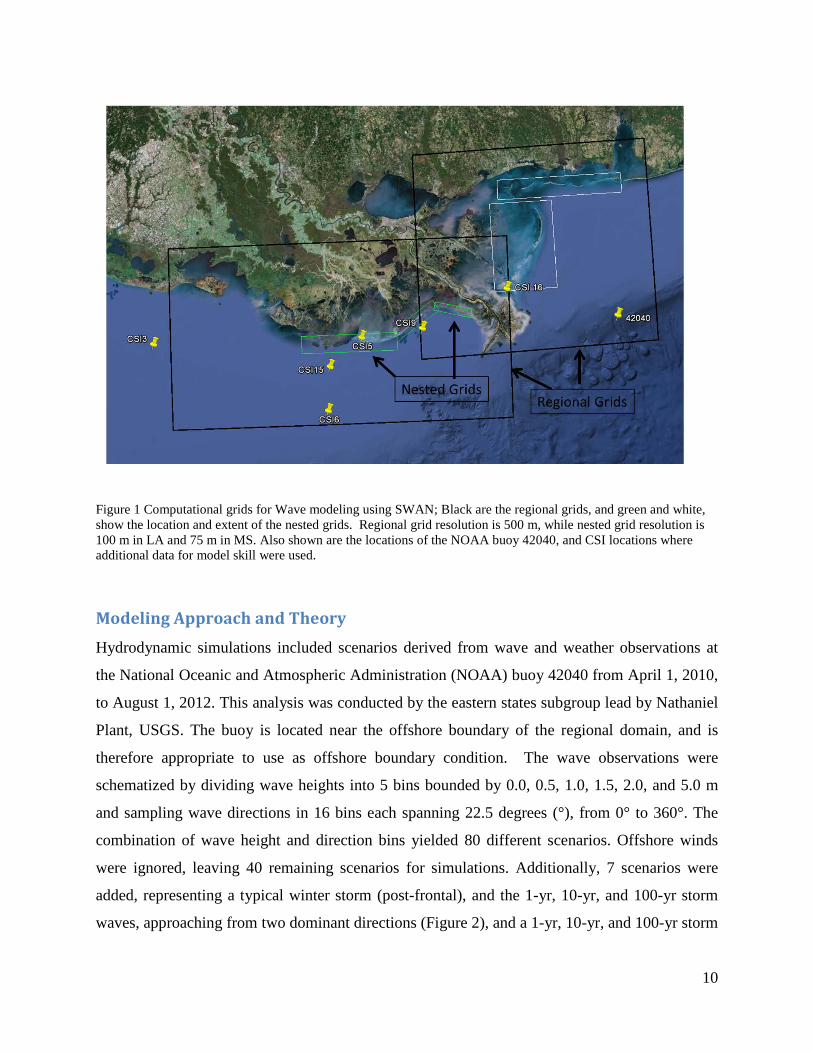
List of Figures Figure 1 Computational grids for Wave modeling using SWAN; Black are the regional grids, and

green and white, show the location and extent of the nested grids. Regional grid resolution

is 500 m, while nested grid resolution is 100 m in LA and 75 m in MS. Also shown are the

locations of the NOAA buoy 42040, and CSI locations where additional data for model

skill were used...................................................................................................................... 10

Figure 2 Wave analysis to determined wave statistics used in numerical wave modeling; five

magnitude bins, and 16 directions were considered (80 scenarios); ignoring offshore winds,

the simulation matrix was reduced to 40 scenarios. ............................................................ 11

Figure 3 Model computational domain with varying resolution from over 2 Km near the open

boundary to 40 m in tidal passes and waterways. Only wet elements are shown, while the

red boundary indicates the entire domain. ........................................................................... 14

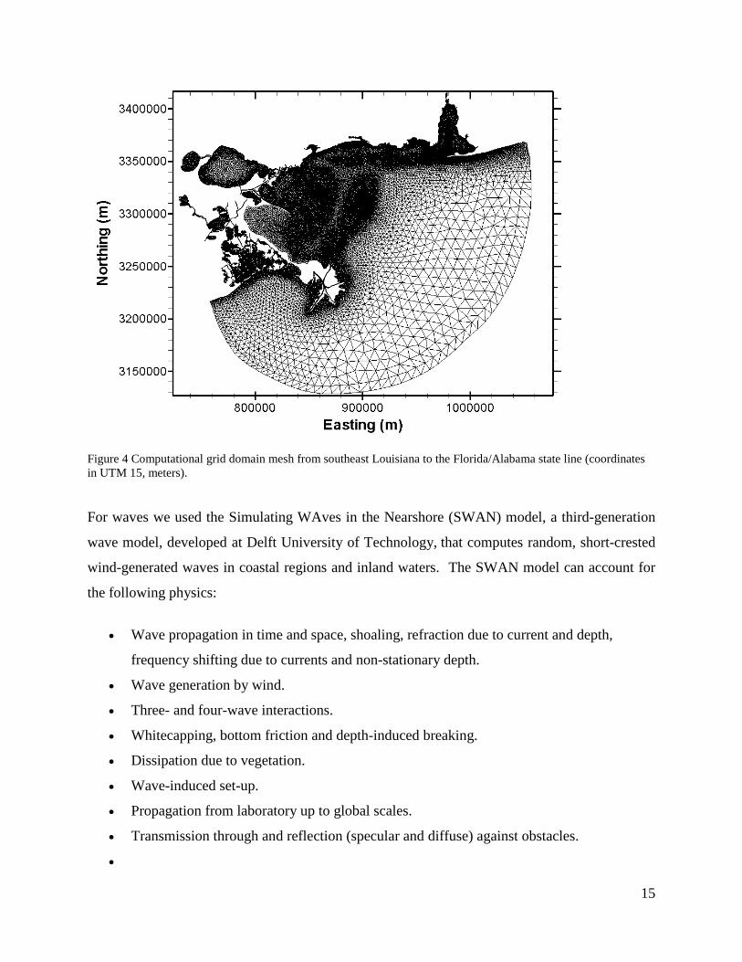
Figure 4 Computational grid domain mesh from southeast Louisiana to the Florida/Alabama state

line (coordinates in UTM 15, meters). ................................................................................. 15

Figure 5 Results from significant wave heights (top panel) and mobility and transport (kg/m/s -

bottom panel) for SRB class 1 resulting from scenario 37 which includes winds from the

southwest. Wave direction is shown with vectors while magnitude of wave height and

transport is shown with contours. ........................................................................................ 24

Figure 6 Results from significant wave heights (top panel) and mobility and transport (kg/m/s -

bottom panel) for SRB class 1 resulting from scenario 40 which includes winds from the

west. Wave direction is shown with vectors while magnitude of wave height and transport

is shown with contours......................................................................................................... 25

Figure 7 Results from significant wave heights (top panel) and mobility and transport (kg/m/s -

bottom panel) for sand resulting from scenario 40 which includes winds from the west.

Wave direction is shown with vectors while magnitude of wave height and transport is

shown with contours. ........................................................................................................... 26

Figure 8 Graphical comparison of model simulated constituents with observations obtained from

harmonic analysis during the validation period for August 2007. ....................................... 29

Figure 9 The inset shows a map of the states surrounding the northern Gulf of Mexico, while the

red box outlines the area shown in the large image. The large image is a map of the

calibration stations within the domain. Table 3 describes these stations in more .............. 31

5

Figure 10 - Meteorological conditions at the NOAA NOS Gulfport Outer Range station (Station

GPOM6 – 8744707) for the period of 3/31/10 to 5/7/10. .................................................... 32

Figure 11 – Comparison of base-case scenario tides (meters) and observed tide data for the

calibration period (3/31/10 to 4/22/10). Calibration efforts focused on good correlation

during the period of 4/16/10 to 4/22/10 (inside the green box) at the following locations

(from top to bottom): Lake Pontchartrain at LUMCON, Rigolets near Lake Pontchartrain,

and Mississippi Sound at St. Joseph Island Light. An adjustment was applied to observed

data to account for vertical datum differences. .................................................................... 33

Figure 12 - Comparison of base-case scenario tides (meters) and observed tide data for the

calibration period (3/31/10 to 4/22/10). Calibration efforts focused on good correlation

during the period of 4/16/10 to 4/22/10 (inside the green box) at the locations (from top to

bottom): D2, NE Bay Gardene near Point à la Hache and Barataria Pass at Grand Isle. An

adjustment was applied to observed data to account for vertical datum differences. .......... 34

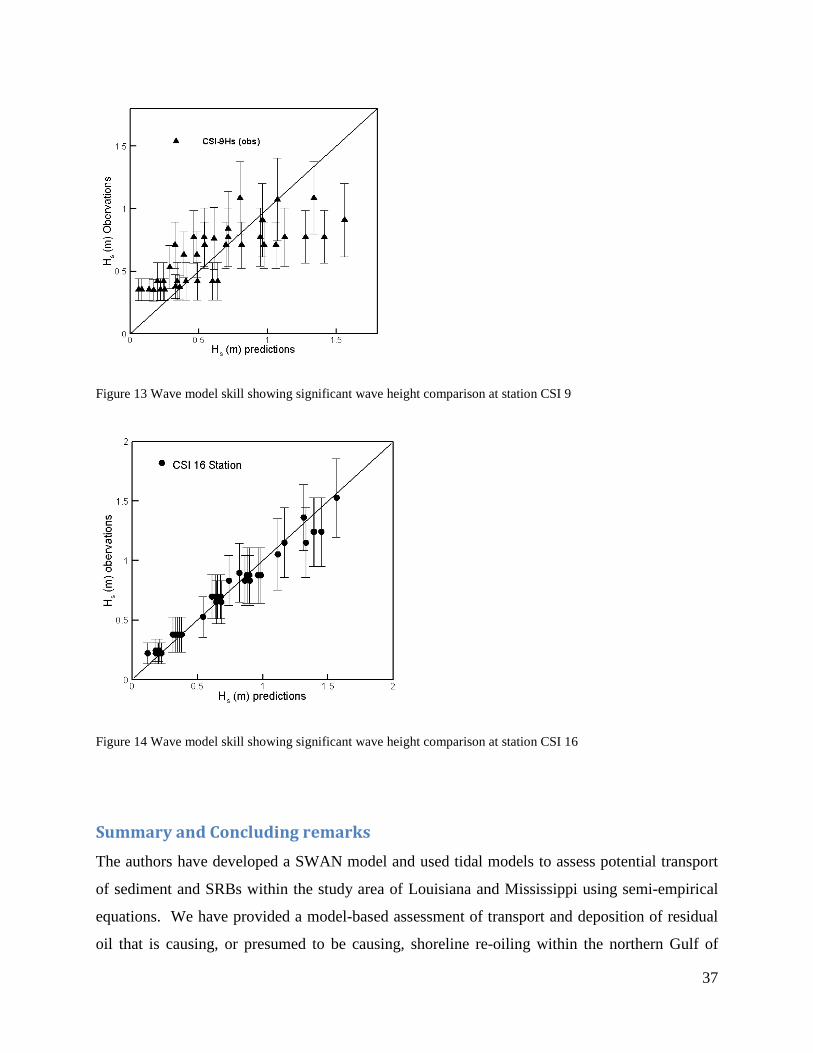
Figure 13 Wave model skill showing significant wave height comparison at station CSI 9 ........ 37

Figure 14 Wave model skill showing significant wave height comparison at station CSI 16 ...... 37

6

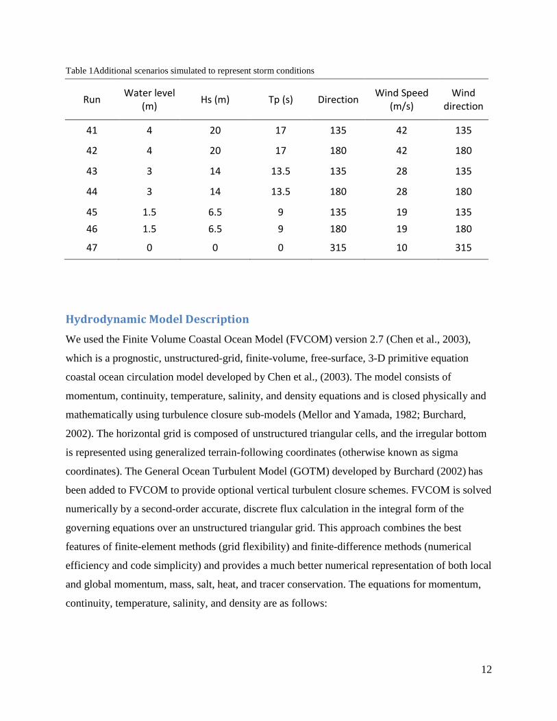
List of Tables Table 1Additional scenarios simulated to represent storm conditions ......................................... 12

Table 2 Critical velocity used in Sediment transport and SRB mobility calculations .................. 19

Table 3 Size classes for natural sediment and SRBs used in the study, with corresponding

density, and critical velocities .............................................................................................. 21

Table 4 Observed and simulated tidal constituents during model validation (values are in meters)

.............................................................................................................................................. 28

Table 5 - Stations used for model calibration. Station name, number, and operating agency, as

well as calibration parameter are provided. Station numbers are in parentheses after station

name. .................................................................................................................................... 31

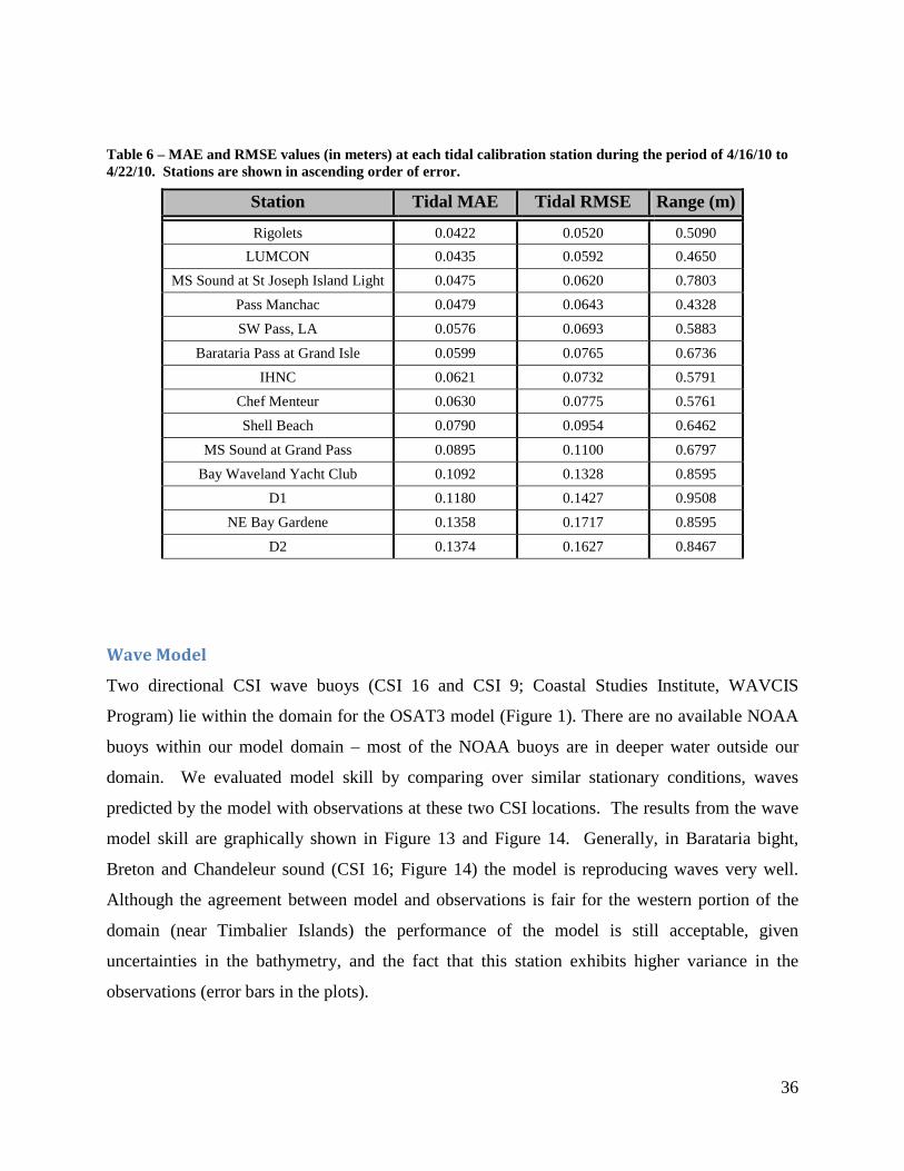
Table 6 – MAE and RMSE values (in meters) at each tidal calibration station during the period

of 4/16/10 to 4/22/10. Stations are shown in ascending order of error. .............................. 36

7

Application of Hydrodynamic and Sediment Transport Models for

Cleanup Efforts Related to the Deepwater Horizon Oil Spill Along the

Coast of Mississippi and Louisiana

By Ioannis Y. Georgiou, Zoe Hughes and Kevin Trosclair

Introduction Residual oil from the Deepwater Horizon spill is found in the shallow surf-zone in the northern

Gulf of Mexico in two primary forms: submerged oil mats and surface residual balls (SRBs).

Mats formed when weathered oil at the surface reached either a shallow environment with

sufficient mixing to facilitate entrainment of sand into the water column to mix with the oil, and

therefore settle, or when surface oil arriving near coastlines was stranded and seeped into the

sand at low tide. Mats encountered as part of the Deepwater Horizon response efforts are

generally meters in cross-shore width, meters to tens of meters in alongshore length, and a few to

tens of centimeters thick. Under high energy events such as winter storms and extratropical

systems, buried mats can be exhumed and pieces of the mats can break off and form SRBs

(Shoreline Cleanup and Assessment Team, oral commun., 2012). The SRBs are observed in the

surf zone and may wash up on beaches. SRBs and mats in the surf zone and on the beach are

targets of ongoing cleanup response efforts. This report presents the results of a subgroup that

developed hydrodynamic and sediment transport models and developed techniques for analyzing

potential SRB redistribution and burial and exhumation to provide a better understanding of

alongshore processes and movement of SRBs along the coastline of Mississippi and Louisiana.

Overall OSAT3 Objectives To provide improved understanding and guidance in support of the operational response to

shoreline re-oiling, Operational Science Advisory Team (OSAT3) undertook five main tasks:

• Evaluate the trends observed in frequency, rate, and potential for remobilization on beach

segments in the areas affected by re-oiling.

8

• Determine and record the locations and typical shoreline profiles and morphology for likely

sources of residual oil or origin of the SRBs.

• Define or determine the mechanisms whereby re-oiling phenomena may be occurring.

• Investigate the potential for mitigation actions that may be taken to reduce these potential

occurrences and, evaluate the feasibility of the mitigation actions and net environmental

benefit.

• Recommend a path forward to reach shoreline cleanup completion plan guidelines or

appropriately manage identified areas through alternative methods.

To achieve these overall objectives, the OSAT3 team collected and analyzed shoreline cleanup

data (for example, SRB and mat recovery, high resolution stereoscopic images) and geomorphic

data (beach profiles, aerial imagery, shorelines, topography, and bathymetry) and conducted

numerical modeling analysis of waves, water levels, currents, local surficial sediment, and SRB

mobility and transport. This report specifically addresses the numerical modeling aspect of the

OSAT3 objectives along the coastline of Louisiana and Mississippi; overall OSAT3 findings are

not within the scope of the analysis of this report.

Objectives of the Hydrodynamic and Sediment Transport Models This report documents the approach, results, and discussion from the LA/MS OSAT3 subgroup

(hereafter LAMS-O3) that developed hydrodynamic and sediment (including SRBs) transport

models to provide better understanding and prediction of alongshore processes and movement of

SRBs. This report addresses the work for Louisiana and Mississippi coastlines. The specific

objectives of this subgroup’s effort were to

• identify spatial patterns in alongshore current directions and velocity

9

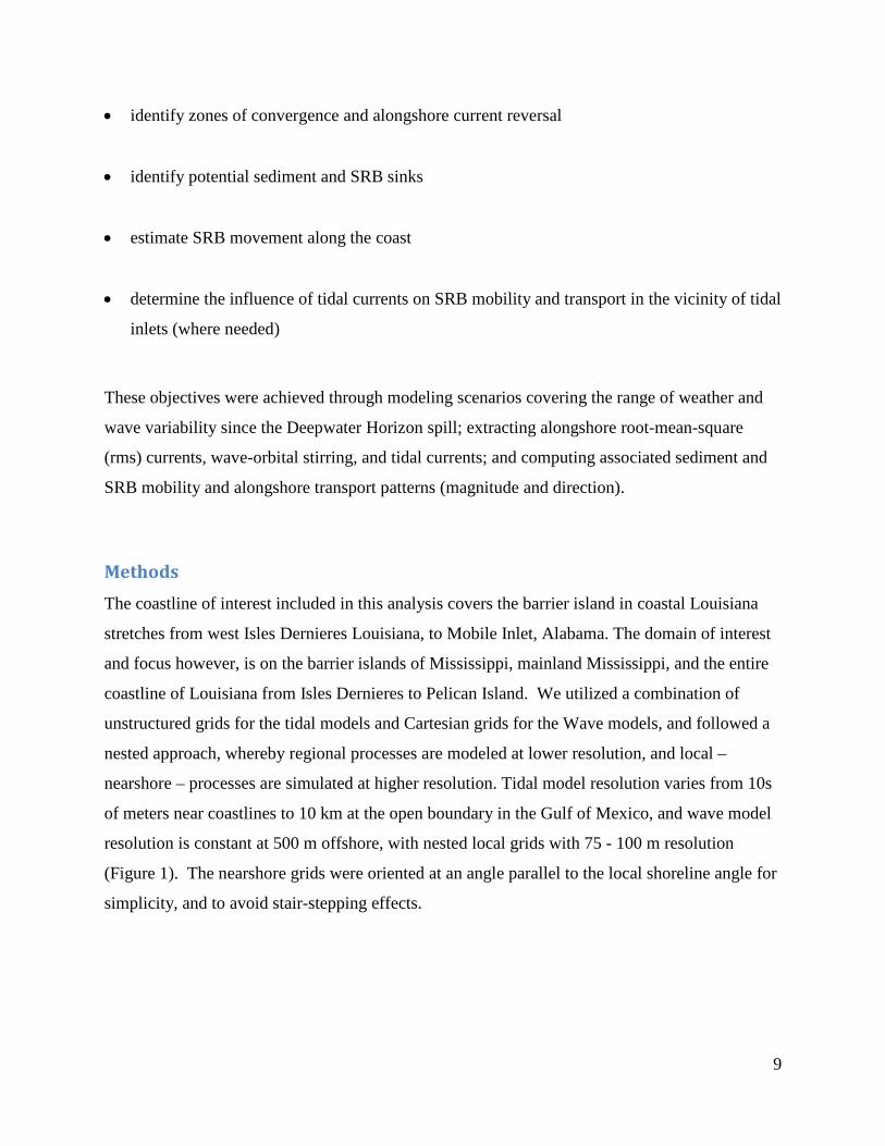
• identify zones of convergence and alongshore current reversal

• identify potential sediment and SRB sinks

• estimate SRB movement along the coast

• determine the influence of tidal currents on SRB mobility and transport in the vicinity of tidal

inlets (where needed)

These objectives were achieved through modeling scenarios covering the range of weather and

wave variability since the Deepwater Horizon spill; extracting alongshore root-mean-square

(rms) currents, wave-orbital stirring, and tidal currents; and computing associated sediment and

SRB mobility and alongshore transport patterns (magnitude and direction).

Methods The coastline of interest included in this analysis covers the barrier island in coastal Louisiana

stretches from west Isles Dernieres Louisiana, to Mobile Inlet, Alabama. The domain of interest

and focus however, is on the barrier islands of Mississippi, mainland Mississippi, and the entire

coastline of Louisiana from Isles Dernieres to Pelican Island. We utilized a combination of

unstructured grids for the tidal models and Cartesian grids for the Wave models, and followed a

nested approach, whereby regional processes are modeled at lower resolution, and local –

nearshore – processes are simulated at higher resolution. Tidal model resolution varies from 10s

of meters near coastlines to 10 km at the open boundary in the Gulf of Mexico, and wave model

resolution is constant at 500 m offshore, with nested local grids with 75 - 100 m resolution

(Figure 1). The nearshore grids were oriented at an angle parallel to the local shoreline angle for

simplicity, and to avoid stair-stepping effects.

10

Figure 1 Computational grids for Wave modeling using SWAN; Black are the regional grids, and green and white, show the location and extent of the nested grids. Regional grid resolution is 500 m, while nested grid resolution is 100 m in LA and 75 m in MS. Also shown are the locations of the NOAA buoy 42040, and CSI locations where additional data for model skill were used.

Modeling Approach and Theory Hydrodynamic simulations included scenarios derived from wave and weather observations at

the National Oceanic and Atmospheric Administration (NOAA) buoy 42040 from April 1, 2010,

to August 1, 2012. This analysis was conducted by the eastern states subgroup lead by Nathaniel

Plant, USGS. The buoy is located near the offshore boundary of the regional domain, and is

therefore appropriate to use as offshore boundary condition. The wave observations were

schematized by dividing wave heights into 5 bins bounded by 0.0, 0.5, 1.0, 1.5, 2.0, and 5.0 m

and sampling wave directions in 16 bins each spanning 22.5 degrees (°), from 0° to 360°. The

combination of wave height and direction bins yielded 80 different scenarios. Offshore winds

were ignored, leaving 40 remaining scenarios for simulations. Additionally, 7 scenarios were

added, representing a typical winter storm (post-frontal), and the 1-yr, 10-yr, and 100-yr storm

waves, approaching from two dominant directions (Figure 2), and a 1-yr, 10-yr, and 100-yr storm

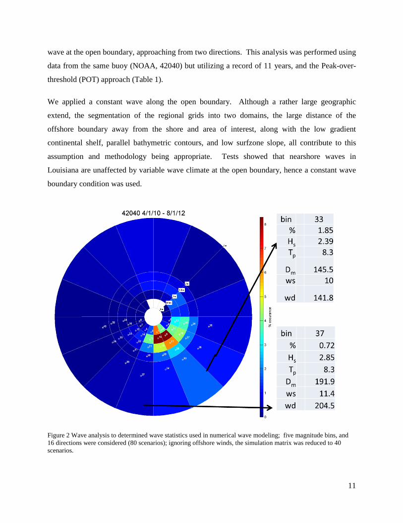
11

wave at the open boundary, approaching from two directions. This analysis was performed using

data from the same buoy (NOAA, 42040) but utilizing a record of 11 years, and the Peak-over-

threshold (POT) approach (Table 1).

We applied a constant wave along the open boundary. Although a rather large geographic

extend, the segmentation of the regional grids into two domains, the large distance of the

offshore boundary away from the shore and area of interest, along with the low gradient

continental shelf, parallel bathymetric contours, and low surfzone slope, all contribute to this

assumption and methodology being appropriate. Tests showed that nearshore waves in

Louisiana are unaffected by variable wave climate at the open boundary, hence a constant wave

boundary condition was used.

Figure 2 Wave analysis to determined wave statistics used in numerical wave modeling; five magnitude bins, and 16 directions were considered (80 scenarios); ignoring offshore winds, the simulation matrix was reduced to 40 scenarios.

12

Table 1Additional scenarios simulated to represent storm conditions

Run Water level (m) Hs (m) Tp (s) Direction Wind Speed

(m/s) Wind

direction

41 4 20 17 135 42 135

42 4 20 17 180 42 180

43 3 14 13.5 135 28 135

44 3 14 13.5 180 28 180

45 1.5 6.5 9 135 19 135 46 1.5 6.5 9 180 19 180

47 0 0 0 315 10 315

Hydrodynamic Model Description We used the Finite Volume Coastal Ocean Model (FVCOM) version 2.7 (Chen et al., 2003),

which is a prognostic, unstructured-grid, finite-volume, free-surface, 3-D primitive equation

coastal ocean circulation model developed by Chen et al., (2003). The model consists of

momentum, continuity, temperature, salinity, and density equations and is closed physically and

mathematically using turbulence closure sub-models (Mellor and Yamada, 1982; Burchard,

2002). The horizontal grid is composed of unstructured triangular cells, and the irregular bottom

is represented using generalized terrain-following coordinates (otherwise known as sigma

coordinates). The General Ocean Turbulent Model (GOTM) developed by Burchard (2002) has

been added to FVCOM to provide optional vertical turbulent closure schemes. FVCOM is solved

numerically by a second-order accurate, discrete flux calculation in the integral form of the

governing equations over an unstructured triangular grid. This approach combines the best

features of finite-element methods (grid flexibility) and finite-difference methods (numerical

efficiency and code simplicity) and provides a much better numerical representation of both local

and global momentum, mass, salt, heat, and tracer conservation. The equations for momentum,

continuity, temperature, salinity, and density are as follows:

13

um FzuK

zxPfv

zuw

yuv

xuu

tu

+

∂∂

∂∂

+∂∂

−=−∂∂

+∂∂

+∂∂

+∂∂

0

1ρ

(1)

vm FzvK

zyPfu

zvw

yvv

xvu

tv

+

∂∂

∂∂

+∂∂

−=+∂∂

+∂∂

+∂∂

+∂∂

0

1ρ

(2)

gzP ρ−=∂∂

(3)

0=∂∂

+∂∂

+∂∂

zw

yv

xu (4)

θθθθθθ Fz

Kzz

wy

vx

ut h +

∂∂

∂∂

=∂∂

+∂∂

+∂∂

+∂∂ (5)

sh FzsK

zzsw

ysv

xsu

ts

+

∂∂

∂∂

=∂∂

+∂∂

+∂∂

+∂∂ (6)

( )s,θρρ = (7)

where x, y, and z are the east, north, and vertical axes of the Cartesian coordinate; u, v, and w are

the x, y, and z velocity components; θ is the potential temperature; s is the salinity; ρ is the

density; P is the pressure; f is the Coriolis parameter; g is the gravitational acceleration; Km is the

vertical eddy viscosity coefficient; and Kh is the thermal vertical eddy diffusion coefficient. Here

Fu, Fv, and Fs represent the horizontal momentum, thermal and salt diffusion terms. For a more

detailed description of model development and other capabilities the reader is directed to Chen et

al., (2003). The model has been used previously in three-dimensional mode due to the episodic

14

and seasonal stratification that the estuary experiences (Poirrier, 1979; Li et al, 2008; Georgiou et

al, 2009) and to capture additional stratification potentially induced near freshwater input

sources. The freely available source code for FVCOM does not readily offer salinity transport

under the two-dimensional mode without code modifications.

Figure 3 Model computational domain with varying resolution from over 2 Km near the open boundary to 40 m in tidal passes and waterways. Only wet elements are shown, while the red boundary indicates the entire domain.

15

Figure 4 Computational grid domain mesh from southeast Louisiana to the Florida/Alabama state line (coordinates in UTM 15, meters).

For waves we used the Simulating WAves in the Nearshore (SWAN) model, a third-generation

wave model, developed at Delft University of Technology, that computes random, short-crested

wind-generated waves in coastal regions and inland waters. The SWAN model can account for

the following physics:

• Wave propagation in time and space, shoaling, refraction due to current and depth,

frequency shifting due to currents and non-stationary depth.

• Wave generation by wind.

• Three- and four-wave interactions.

• Whitecapping, bottom friction and depth-induced breaking.

• Dissipation due to vegetation.

• Wave-induced set-up.

• Propagation from laboratory up to global scales.

• Transmission through and reflection (specular and diffuse) against obstacles.

•

16

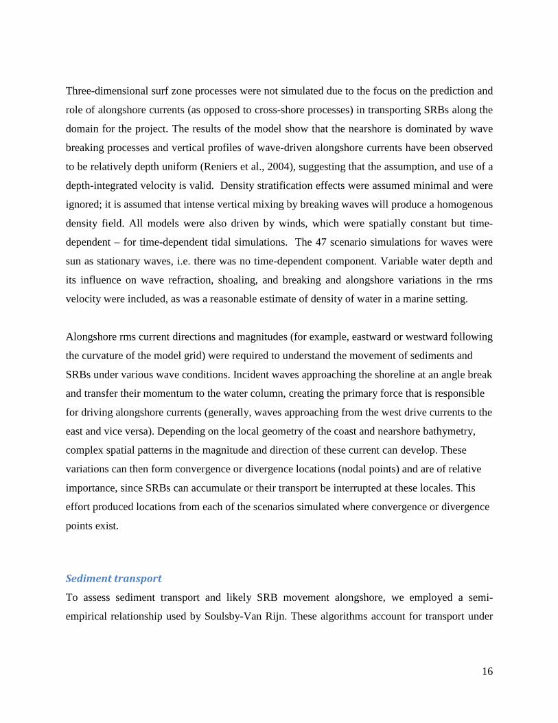
Three-dimensional surf zone processes were not simulated due to the focus on the prediction and

role of alongshore currents (as opposed to cross-shore processes) in transporting SRBs along the

domain for the project. The results of the model show that the nearshore is dominated by wave

breaking processes and vertical profiles of wave-driven alongshore currents have been observed

to be relatively depth uniform (Reniers et al., 2004), suggesting that the assumption, and use of a

depth-integrated velocity is valid. Density stratification effects were assumed minimal and were

ignored; it is assumed that intense vertical mixing by breaking waves will produce a homogenous

density field. All models were also driven by winds, which were spatially constant but time-

dependent – for time-dependent tidal simulations. The 47 scenario simulations for waves were

sun as stationary waves, i.e. there was no time-dependent component. Variable water depth and

its influence on wave refraction, shoaling, and breaking and alongshore variations in the rms

velocity were included, as was a reasonable estimate of density of water in a marine setting.

Alongshore rms current directions and magnitudes (for example, eastward or westward following

the curvature of the model grid) were required to understand the movement of sediments and

SRBs under various wave conditions. Incident waves approaching the shoreline at an angle break

and transfer their momentum to the water column, creating the primary force that is responsible

for driving alongshore currents (generally, waves approaching from the west drive currents to the

east and vice versa). Depending on the local geometry of the coast and nearshore bathymetry,

complex spatial patterns in the magnitude and direction of these current can develop. These

variations can then form convergence or divergence locations (nodal points) and are of relative

importance, since SRBs can accumulate or their transport be interrupted at these locales. This

effort produced locations from each of the scenarios simulated where convergence or divergence

points exist.

Sediment transport

To assess sediment transport and likely SRB movement alongshore, we employed a semi-

empirical relationship used by Soulsby-Van Rijn. These algorithms account for transport under

17

both currents and waves and are summarized herein; a full treatment is available in Soulsby

(1997). The mass transport, Qt (kg/s/m), is given by

ts qQt ρ= (8)

where ρs is the sediment density (2650 kg/m3), and

2.4

2 20.018( ) (1 1.6 tan )t s avg avg rms crD

q A U U U UC

β

= + − −

(9)

is the volumetric transport where Uavg and Ucr are the mean and threshold current velocities

(m/s), Urms is the root-mean-square orbital velocity of the wave (m/s), CD is the drag coefficient

due to current alone, tan β is the non-dimensional bed slope, and As is the total load term. The

total load term is given by

sssbs AAA += (10)

where Asb is the bed-load term and Ass is the suspended load term given by

2.150

6.0*50

])1[(012.0

gdsDdAss −

=−

(11)

and

2.150

2.150

])1[(

)(005.0

gdsh

dhAsb −

= (12)

respectively, in which d50 is the median grain diameter (m), D* is the dimensionless grain

diameter, h is the water depth (m), g is the acceleration due to gravity (m/s2), and s is the relative

density of sediment.

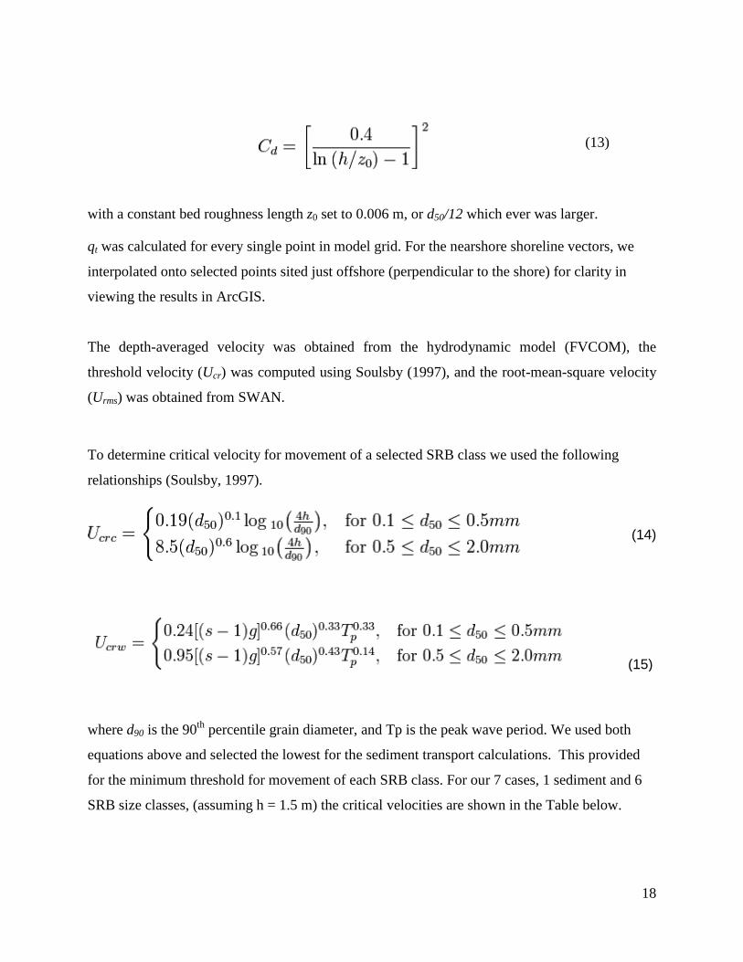
The current drag coefficient is calculated as

18

(13)

with a constant bed roughness length z0 set to 0.006 m, or d50/12 which ever was larger.

qt was calculated for every single point in model grid. For the nearshore shoreline vectors, we

interpolated onto selected points sited just offshore (perpendicular to the shore) for clarity in

viewing the results in ArcGIS.

The depth-averaged velocity was obtained from the hydrodynamic model (FVCOM), the

threshold velocity (Ucr) was computed using Soulsby (1997), and the root-mean-square velocity

(Urms) was obtained from SWAN.

To determine critical velocity for movement of a selected SRB class we used the following

relationships (Soulsby, 1997).

(14)

(15)

where d90 is the 90th percentile grain diameter, and Tp is the peak wave period. We used both

equations above and selected the lowest for the sediment transport calculations. This provided

for the minimum threshold for movement of each SRB class. For our 7 cases, 1 sediment and 6

SRB size classes, (assuming h = 1.5 m) the critical velocities are shown in the Table below.

19

Table 2 Critical velocity used in Sediment transport and SRB mobility calculations SRB class Sediment 1 2 3 4 5 6

Ucrit – currents 0.3482 0.3482 1.0272 1.3955 2.0484 2.6808 3.4206

U crit - waves 0.1942 0.1485 0.4868 0.6559 0.9726 1.3103 1.7653

Hydrodynamic Model Input Data

Bathymetry

Bathymetric data (fig. 1) were obtained from the northern Gulf Coast digital elevation map of the

NOAA National Geophysical Data Center (NGDC; Love and others, 2012). These data, with 30-

m resolution, satisfied the large-scale needs of the domain for the OSAT3 model. We

supplemented the nearshore bathymetry in the vicinity of barrier islands in Louisiana with two

supplemental datasets. One included the 2010 LiDAR dataset for the Mississippi Barrier

(NOAA) and the pre-oiling bathymetry and topography around the Chandeleur Islands from

2010 (courtesy of USGS extreme storms program). Finally, using data from the Barrier Island

Comprehensive Monitoring Program (BICM, Kidinger et al., 2013) we supplemented nearshore

bathymetry in the central coast (Racoon to Sandy point; 2007) and topography using LiDAR

from 2010, for all barriers in Louisiana where data were available (Racoon to Sandy point).

More details on the availability of the bathymetric datasets in BICM can be found here

(http://pubs.usgs.gov/of/2013/1083/).

Waves

Each of the 40 scenarios, and the additional 7 to account for larger storms, were used to force the

model. Wave heights, periods, and directions were used as input to SWAN, with additional

specifications which included an assumed Joint North Sea Wave Project (JONSWAP) spectral

shape (Hasselmann et al., 1973). The directional domain for the wave model covered a full circle

with a resolution of 10° (36 bins in total), and the frequency domain was 0.025 to 1 hertz (Hz)

with logarithmic spacing. The bottom-friction dissipation parameterization of Hasselmann et al.

(1973) was used with a uniform bottom roughness coefficient of 0.067 square meters per second

cubed (m2/s3). Additionally, third-generation physics were activated, accounting for wind wave

20

generation, triad wave interactions, and white capping by the Komen et al. (1984)

parameterization. Depth-induced wave breaking dissipation was included using the Battjes and

Janssen (1978) parameterization with default values for alpha (1) and gamma (0.73).

Winds

Wind velocities were also obtained from NOAA and USGS buoys. Both tidal and wave models

used wind that were constant in space – not spatially varying. For the tidal model simulations,

wind velocities and directions were changing every hour during a fortnight simulation to account

for the maximum tidal currents during spring tides; hence winds where time-dependent, but

constant in space – i.e. the same across the domain. For the Barataria tidal model, winds from

Grand Isle were used, while for the grid covering Breton and Mississippi Sound, winds from the

Grand Pass USGS station were used. These sites have long records, thus they document wind

patterns more effectively and include a large number of storms in their records, and they are also

positioned near open water, and hence are not influenced by land.

SRB and Sand Movement Mobility for SRB classes was based on size and density derived from analysis of SRBs

identified, analyzed and reported by the SCAT teams. The sizes identified for study in the SRB

movement calculations are given in Table 3, and represent a reasonable range of what is picked

up by operations. The mobility was assessed using the previously determined probability of

occurrence, once the critical velocity for each scenario was exceeded (Table 3). For example, if

scenario 1 represents 2 % of the typical year, if at any point in the nested grid the critical velocity

was met, that cell or location was flagged with movement. This information is contained within

the output files. Further, we calculated a weighted probability resulting from all 40 scenarios

representing a typical year. This was conducted for the sediment class, and for each of the SRB

classes. In addition to a weighted probability, we calculated weighted transport. This step is

important because it separates the information provided by the weighted probability to either

significant or non-significant. Although relative terms, this step will isolate an area that appears

to be mobile frequently (i.e. SRBs appear to be mobile based on high probability), but exhibits a

21

very low mass transport rate. The following equations were used to define weighted probability

and weighted mass transport rates.

∑=

=n

k totalk

nkw P

jiPjiP

1 )(

)( )),(

(),( (16)

∑=

=n

k totalk

wknkw P

jiqjiPjiq

1 )(

)( )),(),(

(),( (17)

where Pw and qw are the weighted probability and weighted transport for n scenarios, and i,j are

the grid (spatial) indices.

Table 3 Size classes for natural sediment and SRBs used in the study, with corresponding density, and critical velocities

Class Size (cm) Density**

(kg/m3)

Critical velocity (currents

dominate) Critical velocity

(waves dominate)

Sediment (natural) 0.015* 2650 0.3482 0.1942

SRB1 0.015 2107 0.3482 0.1485

SRB2 0.5 2107 1.0272 0.4868

SRB3 1 2107 1.3955 0.6559

SRB4 2.5 2107 2.0484 0.9726

SRB5 5 2107 2.6808 1.3103

SRB6 10 2107 3.4206 1.7653 *size for natural sand class is based on local knowledge of median grain diameter

**density of SRBs was calculated using grain size data provided by British Petroleum to the USGS subgroup. Specific methodology can be found in the eastern states report.

Metrics for Evaluating Sand and SRB Mobility and Redistribution Patterns Analyses were conducted to determine sediment and SRB movement probability and alongshore

redistribution patterns for SRBs of mobilized size classes for each individual scenario,

22

illustrating the likely mobility and redistribution patterns under the conditions that the scenario

represents. Metrics for hydrodynamics, SRB and sediment movement probability, and

alongshore redistribution for wave scenarios are: significant wave height; tidal current; root-

mean-square (rms) velocity produced by the wave model; and alongshore rms-current

convergences and divergence. Two additional metrics used to assess the overall probability of

mobility and alongshore distribution over the time period of interest, are weighted mobility

probability and weighted potential mass transport rate. Metric calculations are described below.

Significant Wave Height

The significant wave height is calculated by SWAN for each scenario. This parameter is an

output of the model. It is stored in the archive model output but not in the ArcGIS files.

Alongshore rms-current Convergences

The alongshore varying maximum rms-velocity computed by the SWAN wave model was used

to identify flow convergences, indicating locations where the alongshore transport of SRBs

would be disrupted and/or cause possible deposition zones. The rms velocity magnitude, with a

sign for west-east orientation, the two components of the velocity, as well as the coordinates for

convergence and divergence sites for each scenario, is stored in the ArcGIS files.

Weighted Mobility Probability

In addition to individual scenario results, the results from multiple scenarios were combined to

assess persistent patterns in mobility during April 1, 2010, to August 1, 2012. For each scenario,

the mobility map was converted to a binary threshold map delineating locations where the

critical value for mobility had been exceeded (value = 1) and not exceeded (value = 0). For sand

and each SRB class and critical threshold value, an average of this threshold exceedance map

was taken and weighted by the scenario probability of occurrence over the 2-year time period

being considered (Figure 2). The weighted mobility probability varies from 0 to 1, with values

approaching 1 indicating mobility under most wave conditions and values approaching 0

indicating little to no mobility under any wave conditions. The weighted mobility probability is a

measure of the probability that SRBs or sand are mobilized and is analogous to the fraction of

time at each location that mobility occurred over the time period of interest. The mobility ratio

for an individual scenario, however, as previously described, can be any number greater than or

equal to 0, and is the ratio of the stress to the critical threshold value for the single point in time

23

represented by that scenario. The mobility ratio must exceed 1 to indicate mobility under the

conditions of the scenario (see also section titled, SRB and sand movement). Spatial ArcGIS

files showing the weighted mobility and weighted transport are included in a separate format in

ArcGIS for each SRB class and each nested grid.

Tidal Mobility

Tidal mobility is inherent in the selection of a critical velocity. We typically selected a

conservative approach to the current selection, namely those occurring during spring tides. This

would provide a conservative estimate on the movement of SRBs based on tidal currents alone.

However, in most cases, waves dominate the surf zone and spit platforms, especially in micro

tidal settings such as Louisiana and Mississippi, and in almost all situations mobility was

dominated by waves and not tidal currents.

Results Results from all simulations (40 scenarios) were included in ESRI ArcGIS. In addition,

convergence and divergent zones and weighted probability and weighted mass transport are also

included. Output from the wave modeling however is also stored for the entire domain, not just

along the nearshore zones. This represents gigabytes of data stored on data drives and can be

submitted upon request. Example output from spatially varying parameters include among

others, significant wave height, maximum wave height, period, energy dissipation terms, wave

skewness, wave direction, depth, water level, bottom orbital velocity and rms-velocity.

24

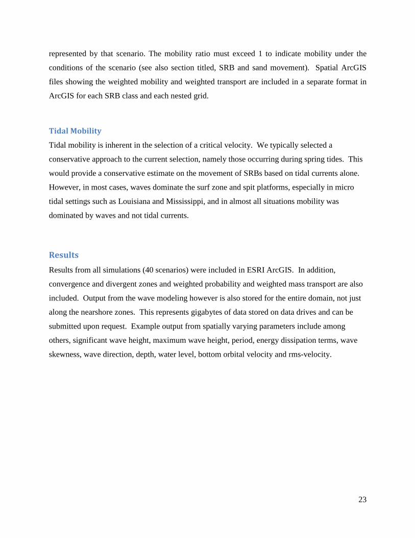
Figure 5 Results from significant wave heights (top panel) and mobility and transport (kg/m/s - bottom panel) for SRB class 1 resulting from scenario 37 which includes winds from the southwest. Wave direction is shown with vectors while magnitude of wave height and transport is shown with contours.

From the above simulation, we notice that offshore bathymetry and specifically ship shoal,

located just offshore (to the south) of the area shown in (Figure 5) modifies the approaching

wave energy such that wave energy arriving at the Isle Dernieres is significantly lower compared

to wave energy arriving at the Timbalier chain. Subsequently, as expected, the potential for

transport (Figure 5; bottom panel) appears to be much higher comparatively. Also notice that the

25

spit platforms, environments that are known to have active transport for longer periods appear

with warm colors, suggesting that these environments do have potentially higher transport, and

therefore mobility, compared to inlets and back barrier bays.

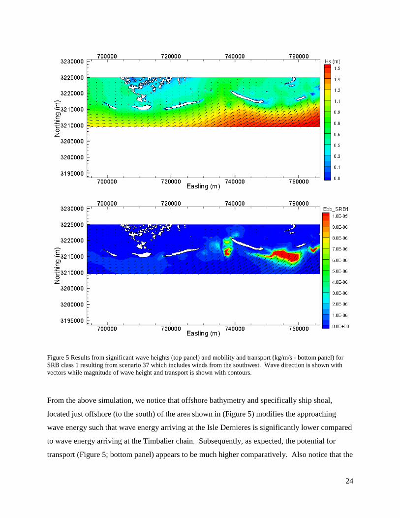
Figure 6 Results from significant wave heights (top panel) and mobility and transport (kg/m/s - bottom panel) for SRB class 1 resulting from scenario 40 which includes winds from the west. Wave direction is shown with vectors while magnitude of wave height and transport is shown with contours.

Similar to scenario 37 (southwest winds) when the islands are subject to winds from the west

(high incident angle) we see evidence of waves generated in the back barrier as well as waves

developing west of the Isle Dernieres barriers, which grow as they travel to the east. This is

evident from the warm colors in Figure 6 (top panel), which shows waves of approximately 0.5

m growing in excess of 1.5 m across the domain (~40 km). These waves, being at high angles,

transform rapidly as they encounter shallow water, seen here to create active transport zones

along spit platforms. Moreover, in these simulations we see wave attack in the back barrier,

generating opposing transport at downdrift locations near the island terminus.

26

Figure 7 Results from significant wave heights (top panel) and mobility and transport (kg/m/s - bottom panel) for sand resulting from scenario 40 which includes winds from the west. Wave direction is shown with vectors while magnitude of wave height and transport is shown with contours.

Similar to west approaching winds in central Louisiana, westerly winds generate waves in

Mississippi sound that grow and eventually approach the islands from the bay side. These types

of conditions are typical during winter storms; in fact, post frontal winds are generally from the

northwest. Figure 7 shows that waves generated in Mississippi Sound can grow to 0.7 m in the

vicinity of Cat Island, while in the back barrier of Ship and Horn Islands, waves can grow in

excess of 1 m. These waves pass near the inlets and recurved spits, and as a result activate spit

platforms, and adjacent shallow water in the vicinity of the recurved spits (Figure 7).

27

Model Evaluation

Tidal Model – Barataria Basin

The model was validated with field data using eight USGS stations within the basin. The station

coverage extends from Barataria Pass, at the seaward entrance of the Basin, to Lake Cataouatche

in the upper basin. An ordinary least squares harmonic analysis with robust fitting was applied to

a yearlong time series of water level data from the field stations. The robust fitting extension

minimizes the effects of storms or seasonal discharge variations and improves the overall

accuracy of the results. The six principal tidal constituents from the field data are O1, K1, P1,

M2, S2, and N2 (Figure 8). These constituents were selected because they were those chosen to

force water levels at the ocean open boundary during the validation simulations (with the

exception of P1, which was not resolved). Finally, a nodal correction was applied to the field

data to correct for the amplitude variations associated with the 18.6 year nodal cycle. For

evaluating the model’s ability to reproduce tidal propagation up-basin, a 28 day period was

selected in August 2007. This period was selected because in addition to tidal elevations

throughout the basin, flow measurements and velocity distribution across the inlets was also

available (FitzGerald et al, 2007). For this period, a harmonic analysis was performed on a 28-

day record of model-simulated water levels at selected model nodes corresponding to the eight

stations, and compared with field results (Table 4, Figure 8).

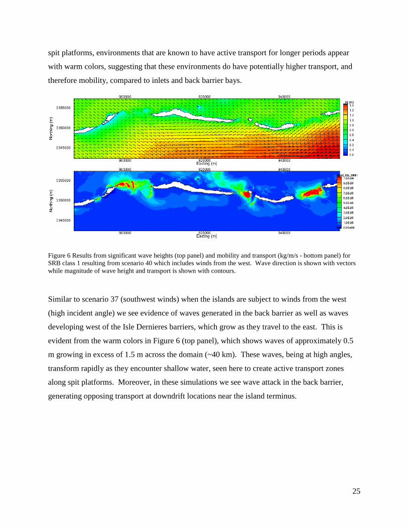
Figure 8 shows that the Basin is dominated by the principal lunar and lunisolar constituents, O1

and K1. These constituents can account for most of the astronomical variations in the Basin and

were, thus the focus of the validation (Georgiou et al, 2010). Once these constituents were

reproduced in the model, which was achieved through variation of the roughness height in the

quadratic friction term of the bottom friction coefficient, no further adjustment was carried out.

The validation was considered satisfactory despite the small disagreements in the principal lunar

constituent M2, which in this area is only 8 % of the principal lunar, or of the order of 1 cm.

Figure 8 shows scatter plots of observed versus simulated constituents for all locations where

harmonic analysis was conducted. The model resolved and reproduced the propagation of the O1

and K1 constituents within 5 mm for almost all locations.

28

Table 4 Observed and simulated tidal constituents during model validation (values are in meters) Site S2 M2 N2 K1 O1

Barataria Pass (model) 0.005 0.010 0.002 0.117 0.117

Barataria Pass (obs) 0.008 0.018 0.006 0.121 0.118

North Grande Terre (model) 0.003 0.007 0.002 0.110 0.112

North Grande Terre (obs) 0.005 0.009 0.003 0.111 0.109

Barataria Bay North (model) 0.003 0.008 0.002 0.110 0.114

Barataria Bay North (obs) 0.005 0.007 0.003 0.109 0.107

Hackberry Bay (model) 0.001 0.005 0.001 0.072 0.070

Hackberry Bay (obs) 0.004 0.006 0.002 0.097 0.096

Barataria Waterway (model) 0.001 0.003 0.001 0.081 0.084

Barataria Waterway (obs) 0.003 0.006 0.002 0.080 0.079

Bay Dos Gris (model) 0.001 0.003 0.000 0.059 0.058

Bay Dos Gris (obs) 0.001 0.003 0.001 0.052 0.054

Little Lake (Cutoff) (model) 0.002 0.002 0.001 0.052 0.053

Little Lake (Cutoff) (obs) 0.001 0.002 0.001 0.044 0.051

Lake Cataouatche (model) 0.001 0.002 0.001 0.026 0.025

Lake Cataouatche (obs) 0.001 0.001 0.001 0.011 0.013

29

Figure 8 Graphical comparison of model simulated constituents with observations obtained from harmonic analysis during the validation period for August 2007.

Tidal Models – Pontchartrain, Mississippi and Breton Sound

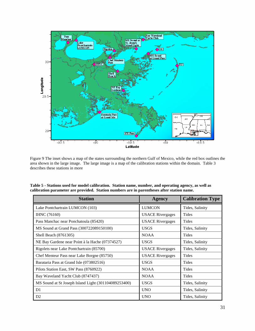
Eleven stations with tides and/or salinity data were chosen for calibration, including stations in

the upper Pontchartrain Estuary, tidal and navigation channels, and open water stations (Figure

6). These stations are operated by NOAA, USGS, NOAA PORTS, LUMCON, and USACE

River gages. The D1 and D2 field data from this study were also used for model calibration.

Table 5 lists the names of stations used, their identification numbers as designated by the

operating agency, and the name of the operating agency. This table also specifies whether each

station was used to calibrate tides (i.e., tidal amplitude and phase) or both tides and salinity.

The model was calibrated to reproduce observed tidal amplitude and phase variations at selected

locations in the NGOM domain.

30

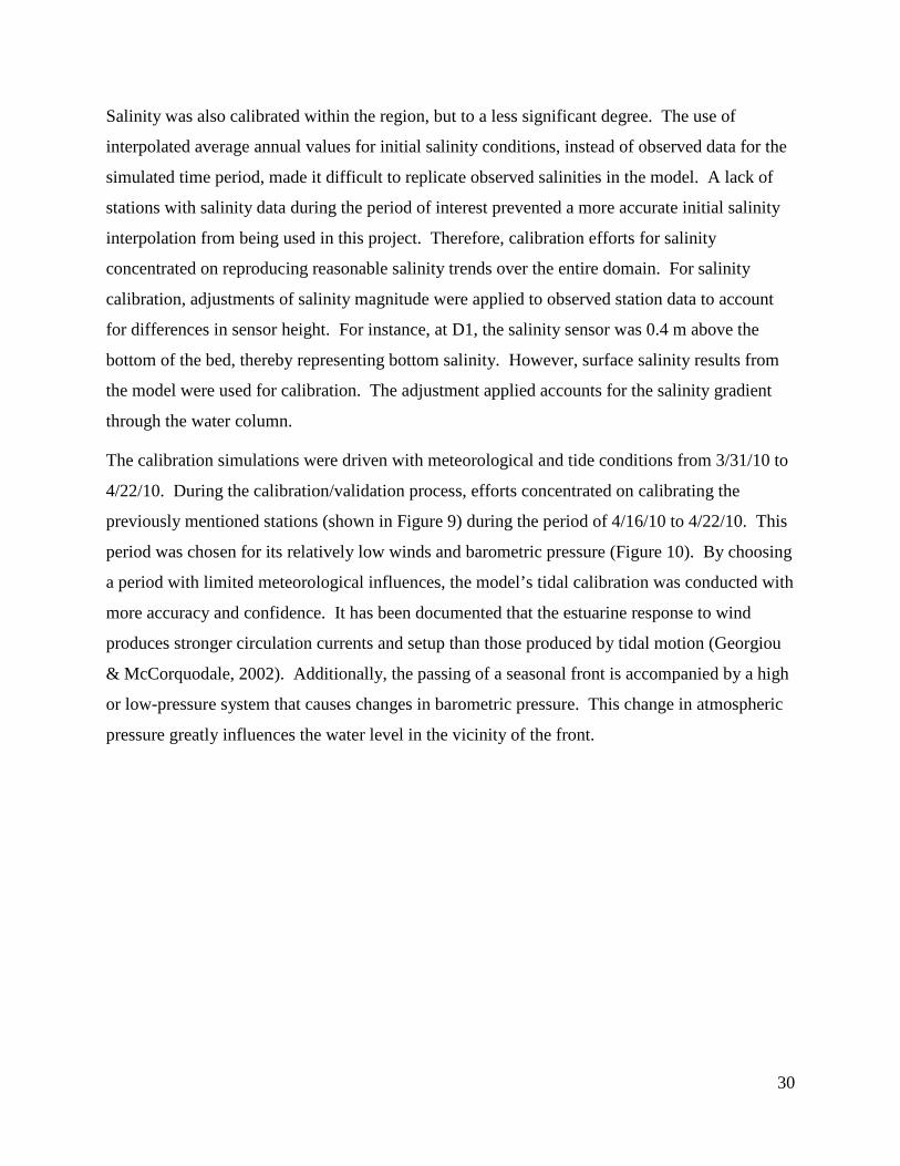
Salinity was also calibrated within the region, but to a less significant degree. The use of

interpolated average annual values for initial salinity conditions, instead of observed data for the

simulated time period, made it difficult to replicate observed salinities in the model. A lack of

stations with salinity data during the period of interest prevented a more accurate initial salinity

interpolation from being used in this project. Therefore, calibration efforts for salinity

concentrated on reproducing reasonable salinity trends over the entire domain. For salinity

calibration, adjustments of salinity magnitude were applied to observed station data to account

for differences in sensor height. For instance, at D1, the salinity sensor was 0.4 m above the

bottom of the bed, thereby representing bottom salinity. However, surface salinity results from

the model were used for calibration. The adjustment applied accounts for the salinity gradient

through the water column.

The calibration simulations were driven with meteorological and tide conditions from 3/31/10 to

4/22/10. During the calibration/validation process, efforts concentrated on calibrating the

previously mentioned stations (shown in Figure 9) during the period of 4/16/10 to 4/22/10. This

period was chosen for its relatively low winds and barometric pressure (Figure 10). By choosing

a period with limited meteorological influences, the model’s tidal calibration was conducted with

more accuracy and confidence. It has been documented that the estuarine response to wind

produces stronger circulation currents and setup than those produced by tidal motion (Georgiou

& McCorquodale, 2002). Additionally, the passing of a seasonal front is accompanied by a high

or low-pressure system that causes changes in barometric pressure. This change in atmospheric

pressure greatly influences the water level in the vicinity of the front.

31

Figure 9 The inset shows a map of the states surrounding the northern Gulf of Mexico, while the red box outlines the area shown in the large image. The large image is a map of the calibration stations within the domain. Table 3 describes these stations in more

Table 5 - Stations used for model calibration. Station name, number, and operating agency, as well as calibration parameter are provided. Station numbers are in parentheses after station name.

Station Agency Calibration Type

Lake Pontchartrain LUMCON (103) LUMCON Tides, Salinity IHNC (76160) USACE Rivergages Tides Pass Manchac near Ponchatoula (85420) USACE Rivergages Tides

MS Sound at Grand Pass (300722089150100) USGS Tides, Salinity Shell Beach (8761305) NOAA Tides NE Bay Gardene near Point à la Hache (07374527) USGS Tides, Salinity Rigolets near Lake Pontchartrain (85700) USACE Rivergages Tides, Salinity

Chef Menteur Pass near Lake Borgne (85750) USACE Rivergages Tides Barataria Pass at Grand Isle (073802516) USGS Tides Pilots Station East, SW Pass (8760922) NOAA Tides Bay Waveland Yacht Club (8747437) NOAA Tides

MS Sound at St Joseph Island Light (301104089253400) USGS Tides, Salinity D1 UNO Tides, Salinity D2 UNO Tides, Salinity

32

Figure 10 - Meteorological conditions at the NOAA NOS Gulfport Outer Range station (Station GPOM6 – 8744707) for the period of 3/31/10 to 5/7/10.

Bottom roughness (z0b) were adjusted during the calibration phase to correct inland tidal

propagation and attenuation (Schindler 2010). For instance, when tidal amplitudes were

represented accurately at Grand Pass but under-represented at Pass Manchac, the bottom

roughness was reduced. By reducing the bottom roughness, tidal amplitudes were less

33

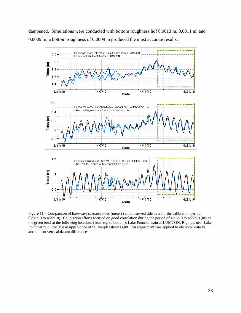
dampened. Simulations were conducted with bottom roughness hof 0.0013 m, 0.0011 m, and

0.0009 m; a bottom roughness of 0.0009 m produced the most accurate results.

Figure 11 – Comparison of base-case scenario tides (meters) and observed tide data for the calibration period (3/31/10 to 4/22/10). Calibration efforts focused on good correlation during the period of 4/16/10 to 4/22/10 (inside the green box) at the following locations (from top to bottom): Lake Pontchartrain at LUMCON, Rigolets near Lake Pontchartrain, and Mississippi Sound at St. Joseph Island Light. An adjustment was applied to observed data to account for vertical datum differences.

34

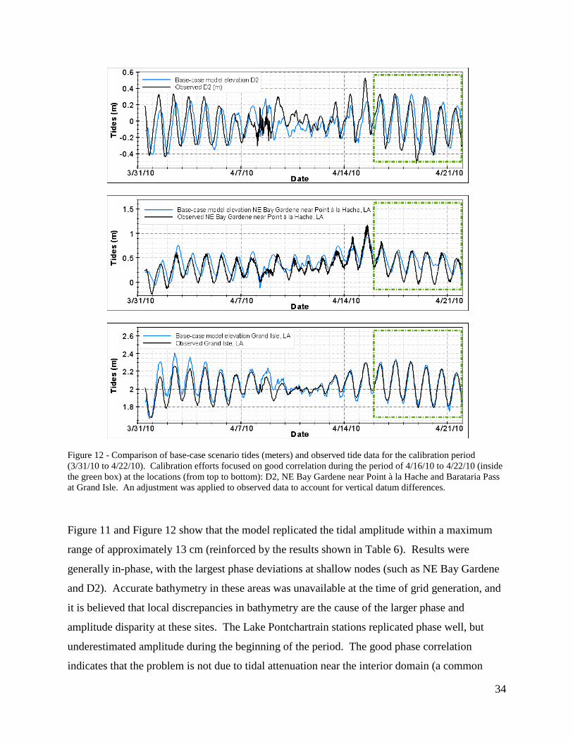
Figure 12 - Comparison of base-case scenario tides (meters) and observed tide data for the calibration period (3/31/10 to 4/22/10). Calibration efforts focused on good correlation during the period of 4/16/10 to 4/22/10 (inside the green box) at the locations (from top to bottom): D2, NE Bay Gardene near Point à la Hache and Barataria Pass at Grand Isle. An adjustment was applied to observed data to account for vertical datum differences.

Figure 11 and Figure 12 show that the model replicated the tidal amplitude within a maximum

range of approximately 13 cm (reinforced by the results shown in Table 6). Results were

generally in-phase, with the largest phase deviations at shallow nodes (such as NE Bay Gardene

and D2). Accurate bathymetry in these areas was unavailable at the time of grid generation, and

it is believed that local discrepancies in bathymetry are the cause of the larger phase and

amplitude disparity at these sites. The Lake Pontchartrain stations replicated phase well, but

underestimated amplitude during the beginning of the period. The good phase correlation

indicates that the problem is not due to tidal attenuation near the interior domain (a common

35

problem in a domain as large as this, but resolved during the calibration phase). It is believed

that these differences in amplitude result from corresponding changes in barometric pressure.

FVCOM does not account for changes in atmospheric pressure, and therefore produces tidal

elevations resulting from wind and astronomical tides only. The aforementioned stations do

replicate tidal signatures during normal periods well (a difference of less than 10 cm), however

all stations poorly simulate the tidal conditions (both phase and amplitude) around the dates of

4/8/10 to 4/9/10. A cold front passed through the area during this time, producing strong

northerly winds and drastic changes in barometric pressures (See Figure 10).

For a numerical comparison of these signals, mean absolute error (MAE) and root-mean-square

error (RMSE) were computed. The MAE was calculated with the equation:

MAE = ∑ �𝑋𝑜𝑏𝑠−𝑋𝑠𝑖𝑚�𝑛𝑖=1

𝑛 (18)

where 𝑋𝑜𝑏𝑠 and 𝑋𝑠𝑖𝑚 represent the observed and simulated data points and 𝑛 is the number of

data points. The RMSE was computed as

RMSE = �∑ �𝑋𝑜𝑏𝑠−𝑋𝑠𝑖𝑚�2𝑛

𝑖=1𝑛 (19)

The range of the observed data provides an important gauge for determining the degree of error.

Smaller ratios of MAE to range indicate that the simulated data has a small degree of deviation

from the observed data. The range is calculated by subtracting the minimum value (Xobs,min) from

the maximum value (Xobs,max) of each observed dataset.

Range = 𝑋𝑜𝑏𝑠,𝑚𝑎𝑥 − 𝑋𝑜𝑏𝑠,𝑚𝑖𝑛 (20)

These values, calculated for the period of 4/16/2010 to 4/22/2010, provide a mathematical

assessment of the base-case scenario validation. Table 6 lists each station and its corresponding

tidal MAE and RMSE values in ascending order of error. The highest tidal MAE and RMSE

rates (Shell Beach to D2 in Table 4) are found at stations where recent bathymetric data were

unavailable and bathymetries had to be estimated for the mesh. Considering this fact, and the

fact that model results will be used to determine trends not magnitudes, the errors at these

stations are within a reasonable range. Stations with recent bathymetries and less complex

topographies (interior domain and channels) had lower error values.

36

Table 6 – MAE and RMSE values (in meters) at each tidal calibration station during the period of 4/16/10 to 4/22/10. Stations are shown in ascending order of error.

Station Tidal MAE

Tidal RMSE

Range (m)

Rigolets 0.0422 0.0520 0.5090 LUMCON 0.0435 0.0592 0.4650

MS Sound at St Joseph Island Light 0.0475 0.0620 0.7803 Pass Manchac 0.0479 0.0643 0.4328 SW Pass, LA 0.0576 0.0693 0.5883

Barataria Pass at Grand Isle 0.0599 0.0765 0.6736 IHNC 0.0621 0.0732 0.5791

Chef Menteur 0.0630 0.0775 0.5761 Shell Beach 0.0790 0.0954 0.6462

MS Sound at Grand Pass 0.0895 0.1100 0.6797 Bay Waveland Yacht Club 0.1092 0.1328 0.8595

D1 0.1180 0.1427 0.9508 NE Bay Gardene 0.1358 0.1717 0.8595

D2 0.1374 0.1627 0.8467

Wave Model

Two directional CSI wave buoys (CSI 16 and CSI 9; Coastal Studies Institute, WAVCIS

Program) lie within the domain for the OSAT3 model (Figure 1). There are no available NOAA

buoys within our model domain – most of the NOAA buoys are in deeper water outside our

domain. We evaluated model skill by comparing over similar stationary conditions, waves

predicted by the model with observations at these two CSI locations. The results from the wave

model skill are graphically shown in Figure 13 and Figure 14. Generally, in Barataria bight,

Breton and Chandeleur sound (CSI 16; Figure 14) the model is reproducing waves very well.

Although the agreement between model and observations is fair for the western portion of the

domain (near Timbalier Islands) the performance of the model is still acceptable, given

uncertainties in the bathymetry, and the fact that this station exhibits higher variance in the

observations (error bars in the plots).

37

Figure 13 Wave model skill showing significant wave height comparison at station CSI 9

Figure 14 Wave model skill showing significant wave height comparison at station CSI 16

Summary and Concluding remarks The authors have developed a SWAN model and used tidal models to assess potential transport

of sediment and SRBs within the study area of Louisiana and Mississippi using semi-empirical

equations. We have provided a model-based assessment of transport and deposition of residual

oil that is causing, or presumed to be causing, shoreline re-oiling within the northern Gulf of

38

Mexico in the form of mixtures of sand and weathered oil, known as surface residual balls

(SRBs). Our results show spatial variations in alongshore rms-currents, including locations

where these gradients result in convergence or divergent zones, areas that will likely accumulate

SRBs if they are in the vicinity. Model results also showed that spit platforms, recurved spits,

and other shallow environments in the vicinity of barrier islands, can be fairly active

environments, and will likely remain as such until nearby sources of SRBs are diminished. In

addition, model results also confirmed that offshore winds, given fetch in excess of 20 km can

generate waves that can reach 0.5 – 1 m in height, which further create active transport along re-

curved spits, and spit platforms. As a result, these environments may either naturally accumulate

SRBs (if a source is present updrift), and are likely to experience burial of material that is already

there (having arrived from a previous transport event). Finally, our model results identify spatial

and temporal variations in the mobility of sand and SRBs.

Modeling results suggest that, under the most commonly observed low-energy wave conditions,

larger SRBs are not likely to move very far alongshore, suggesting small redistribution of larger

SRBs during non-storm conditions. Under storm conditions, however, it is possible for larger

SRBs to be mobilized. However, lag effects and transient energy conditions, as well as normal

conditions, can cause larger SRBs to be either buried, or unburied. This is possible in part due to

the fact that large SRBs are less mobile than sand, which creates additional complexities in

accurately modeling their behavior. In addition to complexities created by lag effects and

transient energy conditions, at large size classes (for instance SRBs of 10 cm) the transport

algorithms have lower performance because limited datasets exist to validate the predictions.

References Battjes, J.A., and Janssen, J.P.F.M., 1978, Energy loss and set-up due to breaking of random

waves, chap. 32 of Coastal engineering—1978: Conference on Coastal Engineering, 16th,

Hamburg, Germany, 1978, Proceedings, p. 569–587.

39

Booij, N., Ris, R.C., and Holthuijsen, L.H., 1999, A third-generation wave model for coastal

regions—1. Model description and validation: Journal of Geophysical Research, v. 104, no.

C4, p. 7649–7666.

Bottacin-Busolin, Andrea, Tait, Simon, Marion, Andrea, Chegini, Amir, and Tregnaghi, Matteo,

2008, Probabilistic description of grain resistance from simultaneous flow field and grain

motion measurements: Water Resources Research, v. 44, no. 9, WO9419, 12 p.

Boyer, D.L., Fernando, H.J.S., and Voropayev, S.I., 2002, The dynamics of cobbles in and near

the surf zone: Arizona State University, 37 p., accessed September 5, 2012, at

http://www.dtic.mil/dtic/tr/fulltext/u2/a412197.pdf.

Burchard, H., 2002. Applied turbulence modeling in marine waters. Springer:Berlin-Heidelberg-

New York-Barcelona-Hong Kong-London-Milan Paris-Tokyo, 215pp.

Chen, C. H. Liu, R. C. Beardsley, 2003. An unstructured, finite-volume, three-dimensional,

primitive equation ocean model: application to coastal ocean and estuaries. J. Atm. &Oceanic

Tech., 20, 159-186.

Davies, A.G., Soulsby, R.L., and King, H.L., 1988, A numerical model of the combined wave

and current bottom boundary layer: Journal of Geophysical Research—Oceans, v. 93, no. C1,

January 15, p. 491–508.

FitzGerald, D., Howes, N., Kulp, M., Hughes, Z., Georgiou, I.Y., and Penland, S., 2007,

Impacts of rising sea level to backbarrier wetlands, tidal inlets, and barriers: Barataria Coast,

Louisiana, Coastal Sediments 07, Conference Proceedings, CD-ROM13.

Georgiou, I.Y., McCorquodale, J. A., Schindler, J., Retana A.G., FitzGerald, D.M., Hughes, Z.,

Howes, N., 2009, Impact of Multiple Freshwater Diversions on the Salinity Distribution in the

Pontchartrain Estuary under Tidal Forcing, Journal of Coastal Research, Vol. 54, pp. 59 – 70.

Georgiou, I.Y., McCorquodale, J.A., Nepani, J., Howes, N., Hughes, Z., FitzGerald, D.M.,

Schindler, J.K., 2010, Modeling the hydrodynamics of diversions into Barataria Bay, Technical

Final Report submitted to the Lake Pontchartrain Basin Foundation, Pontchartrain Institute for

Environmental Sciences, March 2010, New Orleans, LA 70148, 82 pp.

40

Hasselmann, K., Barnett, T.P., Bouws, E., Carlson, H., Cartwright, D.E., Enke, K., Ewing, J.A.,

Gienapp, H., Hassellman, D.E., Kruseman, P., Meerburg, A., Müller, P., Olbers, D.J., Richter,

K., Sell, W., and Walden, H., 1973, Measurements of wind-wave growth and swell decay

during the joint North Sea wave project (JONSWAP): Hamburg, Germany, Deutsches

Hydrographisches Institut Ergänzungsheft zur Deutschen Hydrogrphischen Zeitscrift Reihe A,

v. 8, no. 12, 95 p., accessed September 5, 2012, at

ftp://ftp.ifremer.fr/ifremer/cersat/products/gridded/wavewatch3/pub/WAVE_PAPERS/Hassel

mann_etal_DHZ1973.pdf.

Komen, G.J., Hasselmann, S., and Hasselmann, K., 1984, On the existence of a fully developed

wind-sea spectrum: Journal of Physical Oceanography, v. 14, no. 8, p. 1271–1285.

Lesser, G.R., Roelvink, J.A., van Kester, J.A.T.M., and Stelling, G.S., 2004, Development and

validation of a three-dimensional morphological model: Journal of Coastal Engineering, v. 51,

nos. 8–9, October, p. 883–915.

Love, M.R., Amante, C.J., Eakins, B.W., and Taylor, L.A., 2012, Digital elevation models of the

northern Gulf coast—Procedures, data sources and analysis: National Oceanic and

Atmospheric Administration Technical Memorandum NESDIS NGDC–59, 43 p., accessed

September 5, 2012, at http://www.ngdc.noaa.gov/dem/squareCellGrid/download/731.

Li, C, N., Walker, A.,Hou , Georgiou I.Y., H., Roberts, E., Laws, E., Weeks, X., Li, J., Crochet.

2008. Circular Plumes in Lake Pontchartrain under Wind Straining, Estuarine Coastal and

Shelf Science, v. 80, iss. 1, p. 161-172.

Mellor, G. L. and T. Yamada, 1982, Development of a turbulence closure model for geophysical

fluid problem. Rev. Geophys. Space. Phys., 20, 851-875.

National Oceanic and Atmospheric Administration, [undated a], Center for Operational

Oceanographic Products and Services—National Ocean Service tide stations, Pensacola Bay,

41

FL (8729840),: National Oceanic and Atmospheric Administration, accessed September 5,

2012, at http://tidesandcurrents.noaa.gov/index.shtml.

National Oceanic and Atmospheric Administration, [undated b], Digital coast—2010 U.S. Army

Corps of Engineers topo/bathy lidar—Alabama and Florida: National Oceanic and

Atmospheric Administration, accessed September 5, 2012, at

http://www.csc.noaa.gov/dataviewer/.

National Oceanic and Atmospheric Administration, [undated c], National Data Buoy Center—

Meteorological/ocean stations 42040: National Oceanic and Atmospheric Administration,

accessed September 5, 2012, at http://www.ndbc.noaa.gov/.

Poirrier, M.A., 1979., Studies of stratification in southern Lake Pontchartrain near the Inner

Harbor Navigational Canal. Proceedings of the Louisiana Academy of Sciences, 41:26-35

Reniers, A.J.H.M., Thornton, E.B., Stanton, T.P., and Roelvink, J.A., 2004, Vertical flow

structure during Sandy Duck—Observations and modeling: Coastal Engineering, v. 51, no. 3,

p. 237–260.

Ris, R.C., Holthuijsen, L.H., and Booij, N., 1999, A third-generation wave model for coastal

regions—2. Verification: Journal of Geophysical Research, v. 104, no. C4, p. 7667–7681.

Schindler, Jennifer, "Estuarine Dynamics as a Function of Barrier Island Transgression and

Wetland Loss: Understanding the Transport and Exchange Processes" (2010). University of

New Orleans Theses and Dissertations. Paper 1260.

Soulsby, R.L., 1997, Dynamics of marine sands—A manual for practical applications: London,

Thomas Telford Publications, 249 p.

Soulsby, R.L., and Damgaard, J.S., 2005, Bedload sediment transport in coastal waters: Coastal

Engineering, v. 52, no. 8, August, p. 673–689.