Embed Size (px)
Citation preview
Appendix D
Summary of Hydrodynamic, Sediment Transport, and Wave Modeling
325 S. Lake Avenue, Suite 700
Duluth, MN 55802-2323
Phone: 218.529.8200
Fax: 218.529.8202
Appendix D
Summary of Hydrodynamic, Sediment Transport, and Wave
Modeling
Spirit Lake Sediment Site
Prepared for
U. S. Steel Corporation
November 2014
P:\Duluth\23 MN\69\23691125 St Louis River Duluth Works Sediment\WorkFiles\P_Feasibility Study\FS-Report\Appendices\04_Appendix
D_Hydrodynamic and Morphodynamic Modeling Technical Memo\Appendix D_withUSScomments_112114.docx
i
Summary of Hydrodynamic, Sediment Transport,
and Wave Modeling
Spirit Lake Sediment Site
November 2014
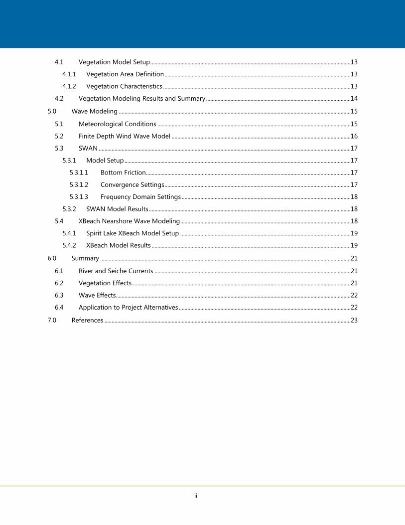
Contents
1.0 Introduction ........................................................................................................................................................................... 1
1.1 Spirit Lake Physical System ......................................................................................................................................... 1
1.1.1 Bathymetric Scans ..................................................................................................................................................... 2
1.1.2 Hydrodynamic Data .................................................................................................................................................. 2
1.1.2.1 River Discharge ................................................................................................................................................. 3
1.1.2.2 Water Level ........................................................................................................................................................ 3
1.1.2.3 Flow Velocity ..................................................................................................................................................... 4
1.1.2.4 Wave Height ...................................................................................................................................................... 4
1.1.3 Meteorological Data ................................................................................................................................................ 4
1.1.4 Sediment Data ............................................................................................................................................................ 5
2.0 Modeling Software .............................................................................................................................................................. 6
2.1 Delft3D ................................................................................................................................................................................ 6
2.2 SWAN/XBeach .................................................................................................................................................................. 6
3.0 Morphodynamic Model (FLOW and SED ONLINE) ................................................................................................ 7
3.1 Computational Grid and Bathymetry ...................................................................................................................... 7
3.2 Boundary Conditions ..................................................................................................................................................... 7
3.2.1 Hydrodynamics .......................................................................................................................................................... 7
3.2.2 Sediment Load ............................................................................................................................................................ 8
3.2.3 Bed Roughness ........................................................................................................................................................... 9
3.2.4 Sediment Characteristics ........................................................................................................................................ 9
3.3 Morphodynamic Model Results ..............................................................................................................................10
3.3.1 June 2012 Flood Scenario ....................................................................................................................................10
3.3.2 Fall 2011 Low Flow Scenario ...............................................................................................................................10
3.3.3 Sensitivity Analysis ..................................................................................................................................................11
3.4 Summary ..........................................................................................................................................................................12
4.0 Vegetation Modeling .......................................................................................................................................................13
ii
4.1 Vegetation Model Setup ............................................................................................................................................13
4.1.1 Vegetation Area Definition ..................................................................................................................................13
4.1.2 Vegetation Characteristics ...................................................................................................................................13
4.2 Vegetation Modeling Results and Summary .....................................................................................................14
5.0 Wave Modeling ..................................................................................................................................................................15
5.1 Meteorological Conditions .......................................................................................................................................15
5.2 Finite Depth Wind Wave Model .............................................................................................................................16
5.3 SWAN ................................................................................................................................................................................17
5.3.1 Model Setup ..............................................................................................................................................................17
5.3.1.1 Bottom Friction ...............................................................................................................................................17
5.3.1.2 Convergence Settings ..................................................................................................................................17
5.3.1.3 Frequency Domain Settings ......................................................................................................................18
5.3.2 SWAN Model Results .............................................................................................................................................18
5.4 XBeach Nearshore Wave Modeling .......................................................................................................................18
5.4.1 Spirit Lake XBeach Model Setup .......................................................................................................................19
5.4.2 XBeach Model Results ...........................................................................................................................................19
6.0 Summary ...............................................................................................................................................................................21
6.1 River and Seiche Currents .........................................................................................................................................21
6.2 Vegetation Effects.........................................................................................................................................................21
6.3 Wave Effects ....................................................................................................................................................................22
6.4 Application to Project Alternatives ........................................................................................................................22
7.0 References ............................................................................................................................................................................23
iii
List of Tables
Table 1 Vegetation species and characteristics.................................................................................................... 14
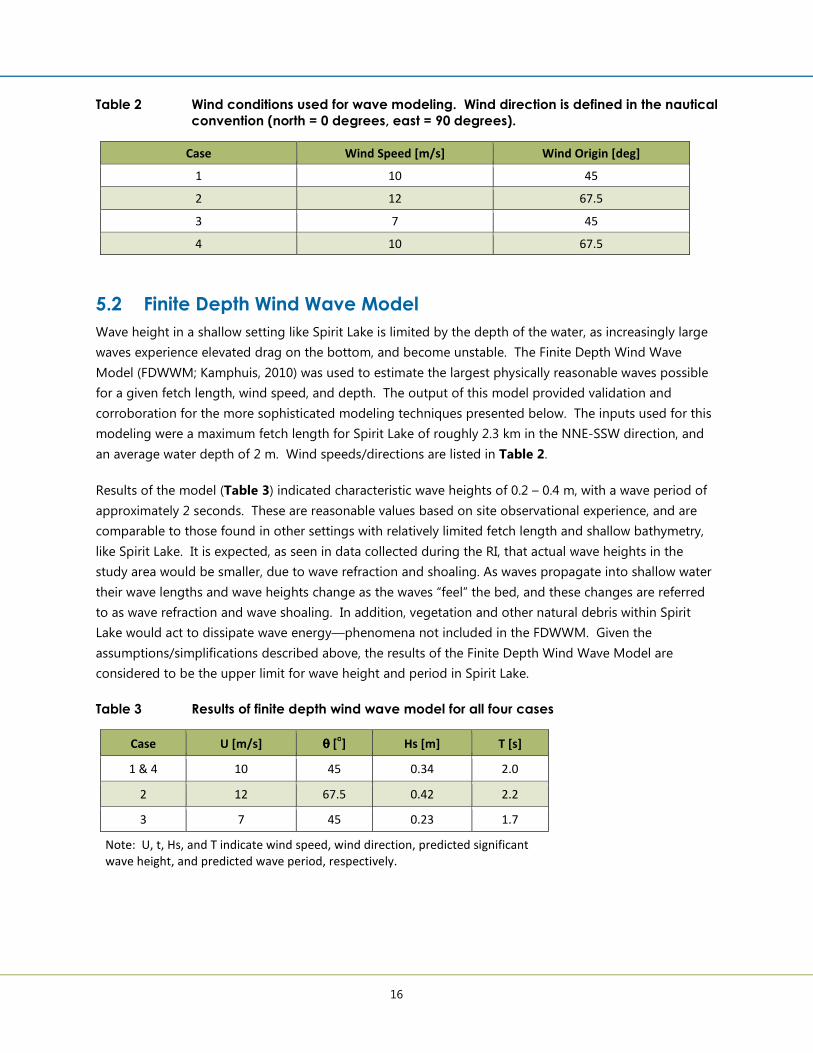
Table 2 Wind conditions used for wave modeling. Wind direction is defined in the nautical
convention (north = 0 degrees, east = 90 degrees). ......................................................................... 16
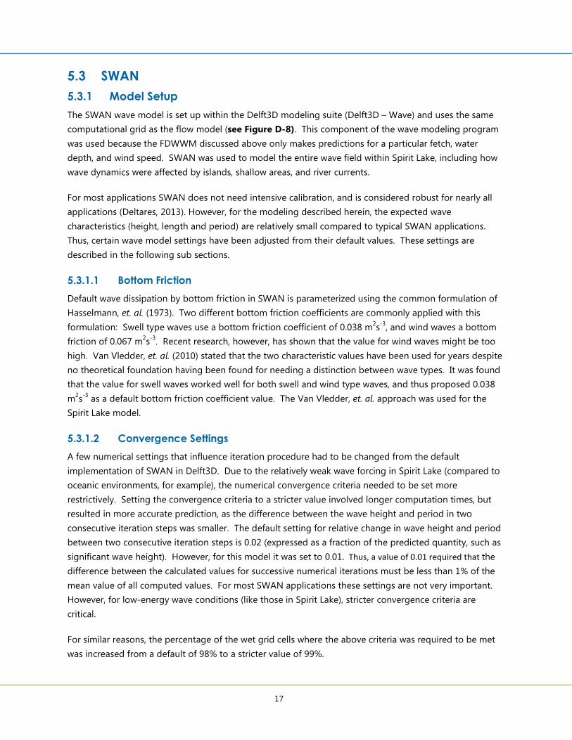
Table 3 Results of finite depth wind wave model for all four cases ............................................................ 16
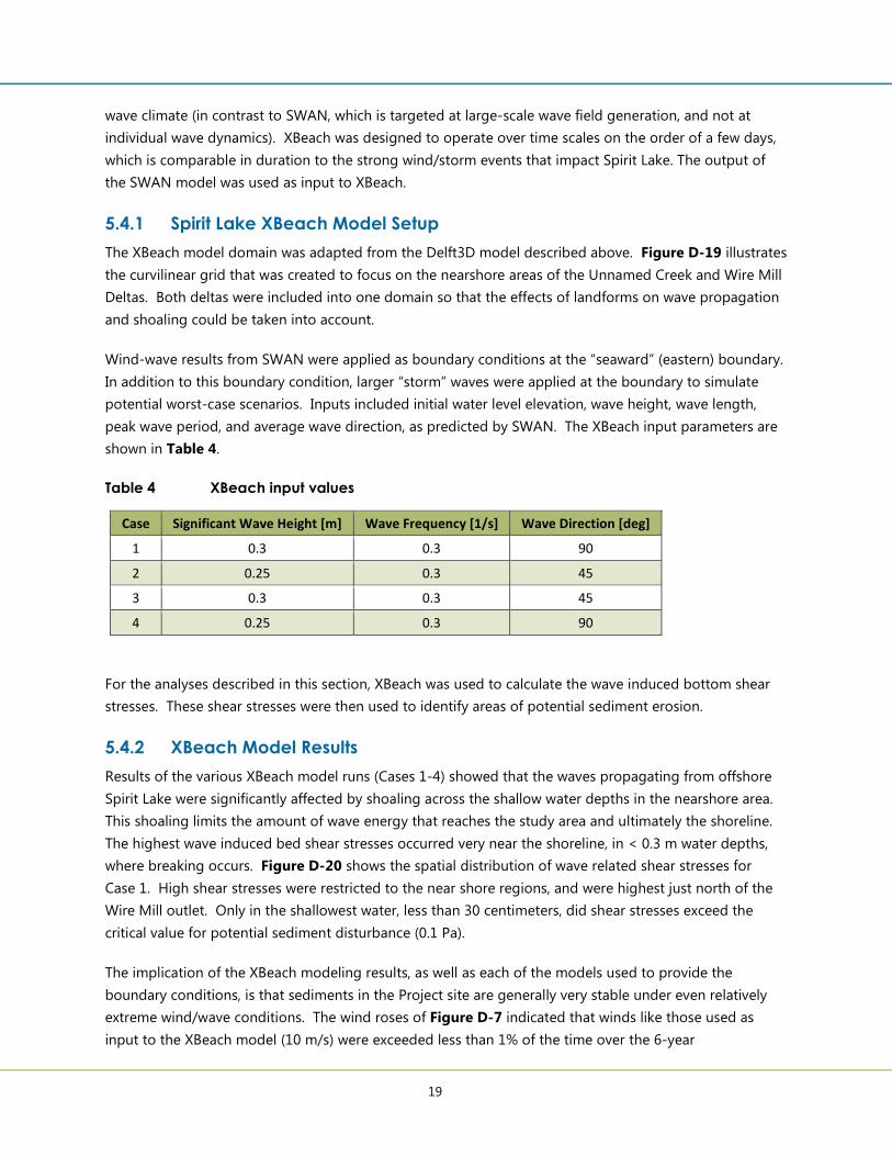
Table 4 XBeach input values ........................................................................................................................................ 19
List of Figures
Figure D-1 2012 Spirit Lake Bathymetry
Figure D-2 Map Showing Bathymetric Change between 2012 and 2011 Surveys
Figure D-3 St. Louis River Discharge History as Measured at Scanlon, Minnesota
Figure D-4 Frequency Spectrum Plot of Lake Superior Water Levels
Figure D-5 Hydrodynamic Data Collection Location Figure
Figure D-6 Vector Plot of Measured Flow Velocities at Unnamed Creek From November 9, 2011 to
November 11, 2011
Figure D-7 Wind Rose for Bong Airport Superior, Wisconsin
Figure D-8 Ternary Diagram of Sediment Data Collected During Geotechnical Evaluation
Figure D-9 Computational Grid for Delft3D Model, with Bathymetry
Figure D-10 Hydrograph for June 2012 Flood Used as Boundary Condition
Figure D-11 Model Predictions for Depth Averaged Velocity during Peak of June 2012 Flood
Figure D-12 Comparison of Modeled Bed Change Predictions with Measured Bed Changes Post June
2012 Flood
Figure D-13 Comparison of Measured and Predicted Water Levels and Velocities for the Low Flow
Modeling Period November 11, 2011 to November 13, 2011
Figure D-14 Map of Vegetation Distribution for Scenario A, as Observed During 2012 Barr Field Survey
Figure D-15 Map of Vegetation Area in Scenario B, Based on 2010 Aerial Photography
Figure D-16 Map of Vegetation Area in Scenario C, Based on Water Depth Less than 1 Meter
Figure D-17 Comparison of Bed Changes to Illustrate Effect of Vegetation
Figure D-18 Wave Characteristic Plot for Wave Modeling Scenario 2
Figure D-19 Computational Grid Used For XBeach Model
Figure D-20 Maximum Bed Shear Stress for XBeach Modeling Case
1
1.0 Introduction
The purpose of this Appendix to the Feasibility Study (FS) is to describe the modeling effort undertaken
by Barr and Deltares to better understand the hydrodynamic and sediment transport processes that
govern Sprit Lake. A number of modeling software packages were used, which are all generally united
under the umbrella of the Delft3D modeling suite developed and maintained by Deltares (2010). Multiple
tools were necessary due to the complex nature of Spirit Lake and the need to consider several important
processes, each of which was best addressed by an effort targeted at that phenomenon. This Appendix
describes each of these modeling efforts, and provides details of how these models were constrained by,
and calibrated to, field observations made during the Sediment Remedial Investigation (RI: Barr, 2013).
The overarching goal of the modeling presented in this Appendix was to provide a tool where the bed
could be modified within Spirit Lake, to predict the functionality of potential Project Alternatives proposed
in the main body of this FS. In other words, a tool that is capable of predicting hypothetical situations,
thus aiding in estimating their feasibility. The conceptual model described in the main body of the
feasibility study was developed from field observations, and served as the starting point for this modeling
effort. Thus, the conceptual model provides the basis for the development of the computational model,
not the converse. This approach (i.e. data before predictions) provides the foundation for hydrodynamic
modeling efforts in Spirit Lake. A model that can be shown to reasonably predict conditions that are
known to exist over a range of conditions provides a sound basis for the simulation of potential future
designs.
The modeling effort was divided into several phases, the details of each are described by sections of this
Appendix:
1. Data analysis and refinement of the RI conceptual model with particular attention to those data
most valuable for model construction and calibration;
2. Development of the numerical morphodynamic (hydrodynamics and sediment transport) model
of Spirit Lake, including calibration to RI data;
3. Addition of wave and vegetation modules to the calibrated morphodynamic model of Spirit Lake,
with additional local wave modeling at specific locations;
4. Evaluation of potential for impacts associated with ice formation; and
5. Additional model analyses with newly available St. Louis River discharge data.
1.1 Spirit Lake Physical System
Spirit Lake is a relatively complex system that is heavily influenced by a number of factors ranging from
the flow of the St. Louis River, to Lake Superior water level, to wind-wave dynamics. A comprehensive
field study was conducted as a part of the RI that captured the details of these processes during both river
flood and low water conditions (Barr, 2013). These data served as the basis for the Site conceptual model
described elsewhere in this FS.

2
This conceptual model and the data serve as the basis for the modeling described in this Appendix. While
a comprehensive review of Site data is not included here, certain aspects of the data are worth reviewing
for clarity. In particular, several data sets are critical for development of model boundary conditions:
1. Bathymetric scans (2011 & 2012)
2. Hydrodynamic data
a. St. Louis River discharge (from Scanlon, MN)
b. Water surface elevation (from on-site measurement station)
c. Flow velocity (from multiple methods at several locations)
d. Wave height
3. Meteorological data
a. Wind speed and direction
4. Sediment data
a. Bed sediment characteristics
b. Water column suspended sediment
These data are summarized briefly in the following sections to provide context for the model boundary
conditions discussed later in this Appendix.
1.1.1 Bathymetric Scans
Bathymetric scanning was undertaken in Spirit Lake in both October 2011 and August 2012. These scans
happen to have occurred on either side of the 500-year return period flood of June 2012, providing a
valuable resource for model development and calibration.
Spirit Lake is relatively shallow throughout its central and western extent, and is characterized by a
relatively deep river channel along the eastern shore of the lake. A dredged channel exists in the north-
central portion of the lake dating to industrial use of the Site, and a deep “hole” is located within the Wire
Mill area in the north west corner near the peninsula (Figure D-1). This was dredged sometime during
the facility operation to create a water intake feature for the former plant operations.
The major flood of June 2012 led to both erosion and deposition of sediment in Spirit Lake. Erosion was
focused in a relatively narrow region in the south-central portion of the lake, and the pattern of this
erosion reflects focusing of flood flow (and associated higher velocity currents) into the main body of the
lake (Figure D-2). As the flood flow entered the main body of the lake significant sediment deposition
occurred throughout the central portion of the lake due to lateral spreading and velocity decrease.
1.1.2 Hydrodynamic Data
Several types of hydrodynamic data were collected during the RI, which serve to both bound the model
runs (e.g. river discharge, water surface elevation) and validate model predictions (e.g. flow velocities and
wave height).
3
1.1.2.1 River Discharge
River discharge data were obtained from both the USGS gauging station located on the St. Louis River at
Scanlon, MN, and from the operations records of the Fond du Lac Dam as provided by Minnesota Power.
While the USGS data provide a long-term record for St. Louis River flow (Figure D-3), the Fond du Lac
Dam data are considered a more realistic representation of the flow through Spirit Lake because the data
are recorded downstream of the two hydropower reservoirs that separate Spirit Lake and Scanlon. Both
data sets have been used for the modeling presented in this Appendix.
The USGS record shows that three major floods (near to or exceeding 1,000 m3/s) have occurred in the
past century—in 1950, 1979, and 2012. Moderate flooding, with discharge between 500 – 1,000 m3/s, is
more common, and has occurred in approximately 1/3 of the past 60 years. Despite these relatively
frequent flood events, the typical summer/fall/winter discharge of the St. Louis River is smaller than 50
m3/s. This discharge record implies two very different regimes occur in Spirit Lake: one where periodic
river floods dominate, and another (much more common) where the river discharge plays a small role in
the overall morphology of the lake.
1.1.2.2 Water Level
The water surface elevation in Spirit Lake is controlled by several factors: Periodic Lake Superior water
level changes, wind/weather related water level changes, and St. Louis River discharge.
The first of these—periodic Lake Superior level variation—is very important in Spirit Lake. Such water
level changes in Spirit Lake are associated with seiche formation in Lake Superior, and are a well-
documented phenomenon caused by oscillation of long-period waves from east to west within the large
lake. Figure D-4 shows a spectral analysis of water level measured in Spirit Lake (Barr 2013) that
indicates how the dominant (most common) frequency of lake level changes occurs every 8 hours, with
less dominant 2 and 4 hour periods. More important for morphological evolution than the lake level,
however, are periods when lake level is changing (i.e.: change in lake level with time, and thus rate of
either draining or filling the lake). In practice, these three frequencies of lake level variation interact with
each other, and lead to a periodic velocity pattern that is discussed in the next sub section.
The weather can cause changes in the level of Spirit Lake, due to phenomena known as either set-up or
set-down of lake level. This behavior is associated with major wind events, and occurs in Spirit Lake due
to sustained uni-directional wind blowing on the surface of Lake Superior. When winds are relatively
strong out of the west for a period of several days, Lake Superior water is pushed to the east, and water
levels can drop in both lakes for several days. Conversely, easterly winds lead to short-term local
increases in lake level. These water level changes are not as important as those associated with seiche
dynamics, as they are less common. However, major storms often lead to larger lake level changes than
does the seiche.
Finally, and most intuitively, high St. Louis River discharge leads to significant (0.1 – 1 m) variation in lake
level. However, increased velocities associated with river flood are typically significantly more important
than lake level in dictating morphologic evolution during such periods.
4
1.1.2.3 Flow Velocity
Flow velocity was documented via two methods: (1) continuous records over several weeks from upward-
oriented acoustic Doppler current profiler (ADCP) devices, and (2) instantaneous measurements at several
points in time, along several transects (Figure D-5). These data show how both river flooding and lake
level changes can affect flow patterns in Spirit Lake.
During low river discharge, overall velocity magnitudes are relatively small—on the order of 0.05 – 0.1
m/s. The dominant velocity pattern during low river discharge is associated with filling and emptying of
Spirit Lake due to Lake Superior seiche. This is reflected as periodic alternation between northward and
southward flow with an approximately 8h period. This phenomenon is particularly evident in a vector plot
of flow velocity near Unnamed Creek between November 9 – 11, 2011 (Figure D-6). During low flow
periods the reduced river flow is directed primarily through the eastern river channel, with velocity
magnitudes generally below the threshold for sediment movement.
Detailed measurements of velocity during the flood of 2012 are not available, due to loss of equipment
during the flood. Two ACDPs were located within the main path of the flow. Buoys attached to the
ADCPs were detached from the ADCPs by the force of the flow and carried downstream where they were
found in the area between Morgan Park and the Riverside Marina. The loss of equipment indicates the
dominance of flood flow in velocity patterns during flood events.
1.1.2.4 Wave Height
Wave data were recorded in four locations (Figure D-5). During the measurement period in the fall of
2011 wave heights in the middle of Spirit Lake only exceeded 0.2 m once, and were typically much smaller
(< 0.05 m). Waves recorded in the central portions of the lake were generally higher than those nearer
the Unnamed Creek and Wire Mill Pond outfall, where wave height never exceeded a few centimeters.
These minimal waves are too small to have an effect on the bottom sediments, though they reflect
relatively mild wave formation conditions present during the measurement period. More sustained
easterly winds could drive larger wind wave formation, but because Spirit Lake is sufficiently small and
shallow that wave heights cannot exceed 0.5m in that water body. A range of potential wave-generating
winds were investigated with the wave modeling presented later in this Appendix.
1.1.3 Meteorological Data
The primary meteorological data needed for the modeling presented in this Appendix are wind direction
and speed. These data in combination with the geometry of the lake are important for modeling wave
influence. The primary source of wind data is the NOAA weather station at the Richard I Bong Airport, in
Superior WI, which is approximately 7.5 km east of Spirit Lake. Additionally, wind direction and speed
were collected at an onsite weather station, though this record is not long enough to produce a
statistically reasonable representation of site conditions through multiple seasons and years. The two
records were compared, however, and indicate that the Bong Airport data reasonably represent the wind
conditions at Spirit Lake.

5
Figure D-7 shows a wind rose derived from the Bong Airport data, which indicates that the record is
dominated by either northeasterly or southwesterly winds. Of these two end members, the northeasterly
winds, which rarely exceed 10 m/s and average approximately 5 m/s, are the most important for wave
formation on the western, impacted, margin of Spirit Lake.
1.1.4 Sediment Data
Two types of sediment data were collected during the RI: 1) bed sediment samples; and 2) suspended fine
grained sediment concentration. The former are useful for parameterizing the potential for sediment
cohesiveness (and thus erosion potential), as well as for parameterizing the overall sediment grain size
distribution in the system. The latter are used to construct a site-specific relationship between river
discharge and suspended sediment load.
The bed of Spirit Lake is dominated by silt and clay sized particles (mean grain size < 62 µm). Coarser
particles (sand sized) were found on the bed in a few places where flow velocities are higher, such as in
the main St. Louis River channel. Determination of whether sediments will behave cohesively or non-
cohesively was made via plotting the grain size data on a ternary sand-silt-clay diagram. Figure D-8
shows that the majority of the bed sediment samples fall in the cohesive field of the diagram (non-
shaded), and that the majority are clay to silt dominated. The implication of sediment grain size data for
the modeling presented in this Appendix is that cohesive bed erosion and sediment transport laws are
appropriate.
6
2.0 Modeling Software
As noted above, several modeling packages/approaches were needed to address the wide range of
important processes that operate within Spirit Lake. Multiple approaches were needed, as no one
modeling tool was capable of evaluating all potential questions that might arise of the Project alternatives
presented in the FS. However, all methods ultimately have a calibrated Delft3D hydrodynamic model at
their core.
2.1 Delft3D
The core numerical model of Spirit Lake used in this FS was developed in the Delft3D software suite—a
fully integrated suite of open source modeling tools that can be used to address a wide range of natural
phenomena and interactions from hydrodynamic processes, to sediment transport, waves, water
chemistry, and vegetation. More information about Delft3D, and the flow equations in particular, can be
found in the Delft3D user manual (Deltares, 2013), or to the Delft3D Open Source Community web portal
(oss.deltares.nl/web/delft3d).
The Delft3D modeling includes several sub components that were used in this analysis (FLOW, SED-
ONLINE, SWAN, and VEG), the parameterization and calibration of which will be discussed as they are
introduced later in the document. Their output forms the boundary condition for the additional modeling
tools described below.
2.2 SWAN/XBeach
The SWAN module of Delft3D, while powerful, is not designed to simulate the effects of individual waves
in the swash zone. Thus, we employed an additional wave modeling tool, XBeach, to make a number of
detailed simulations in regions where impacted sediment exists (Rolevink, et. al., 2010).
7
3.0 Morphodynamic Model (FLOW and SED ONLINE)
A numerical morphodynamic model was developed which uses the hydrodynamic (FLOW) and sediment
transport (SED-ONLINE) modules of Delft3D, as the basis for evaluation of project alternatives.
Hydrodynamics and sediment transport are coupled together in this approach at each time step, so that
the bed is constantly updated during the simulation of hydrodynamic processes. This is particularly
important when significant morphological changes are expected, such as during river flood.
During low flow conditions the hydrodynamic boundary conditions (river currents and waves) were
observed to be relatively small, with flow velocities on the order of 10 cm/s and wave heights of a few
centimeters, as discussed above. These conditions are not likely to mobilize the bed sediments
significantly. However, during flood events the river discharge increases significantly and thus flow
velocities in Spirit Lake become large. Significant morphological changes were measured after the June
2012 flood, with erosion/deposition up to a meter in certain areas of Spirit Lake. Because the present
model was designed to reproduce bed stability and morphological change, the setup and calibration of
the model was focused on matching the pre- to post-flood morphological changes as well as possible.
3.1 Computational Grid and Bathymetry
The model grid was set up to include Spirit Lake and all surrounding areas potentially subject to flooding
during high flow events. Additionally, the model grid was designed to be aligned with likely flow paths, in
this case the main river channel along the eastern shore of Spirit Lake and curvilinear paths through the
central portion of the Lake. Special attention was given to the dredged channel. The resulting
computational grid is shown in Figure D-9. Grid cell edges are generally in the range of 30 – 60 m in
length. This grid alignment was designed to optimize the numerical solution of flows that follow its
geometry and not to promote flow in certain orientations.
The model bathymetry was created using the bed levels measured in October 2011, prior to the flood
event. At locations where bathymetric data were absent, depths were estimated using best engineering
judgment and local knowledge. An initial erodible layer of sediment 0.2 m thick was applied to the bed to
allow for potential erosion below the initial bathymetry.
3.2 Boundary Conditions
3.2.1 Hydrodynamics
The hydrodynamic conditions in Spirit Lake are a result of water level variations, wind shear on the water
surface, and river inflow into the lake. The hydrodynamic forces were imposed as numerical boundaries
via:
1. Water levels at the two northern open boundaries of the domain;
2. River discharge at the southern open boundary; and
3. Wind, translated into drag at the water surface (using the Smith and Bank wind drag formulation).
8
The water level boundary conditions employ the locally measured water levels, while the discharge data at
Scanlon were used as the initial upstream boundary. Additional model runs employ the Fond du Lac
discharge data as their upstream boundary condition. Wind speeds, which are most important for wave-
related model runs, are based on Bong Airport meteorological data.
3.2.2 Sediment Load
One of the most difficult boundary conditions to specify for modeling in river systems is the sediment
load. This estimation is complicated by the fact that sediment loading data are much more difficult to
measure than water discharge, and therefore they are less frequently available. Some data are available
from Scanlon, MN, though they are separated from Spirit Lake by two hydropower reservoirs, and thus are
unlikely to provide an accurate picture of St. Louis River sediment loads at Spirit Lake. Two records were
evaluated as potential boundary conditions:
1. Turbidity measurements that were obtained during the 2012 flood at Scanlon. These data
imply 50,000 – 200,000 m3 of sediment were delivered to Spirit Lake during the flood. This
estimate is much smaller than the total amount of sediment deposition estimated from the
bathymetric surveys (700,000 m3), and therefore implies additional sources of sediment to the
system, particularly during flood. In any case, this discrepancy indicates that the Scanlon turbidity
measurements are not suitable as the upstream boundary condition.
2. Long term sediment concentration measurements at Scanlon. Unfortunately, this time series
did not include the 2012 flood event during model development. The flood of 1979, however,
gives an indication of the concentrations observed for high discharge events. By assuming a linear
relation between discharge and sediment concentration, a sediment concentration for the June
2012 flood event can be estimated. Integrating the sediment load over time with the second
record still leads to an underestimation of the total sediment influx, again implying that additional
sources of sediment exist between Scanlon and Sprit Lake.
An appropriate boundary condition for the model, therefore, requires higher sediment loads than the
Scanlon records would suggest, particularly during times of flood. To estimate the load reasonably, we
relied on the well-understood distinction between wash load (finest grain sizes, never settle in channelized
flow) and suspended bed material load (bed material suspended in the flow during high river discharge).
Thus, some fraction of wash load mud was presumed to travel through the system at all times—low and
flood flow. At higher sediment concentrations (above 50 mg/l) the system was assumed to obtain
additional sediment load via erosion. Preliminary model runs indicated that the sediment load from the
Scanlon record, underestimated the total sediment volume deposited within the model domain during the
2012 Flood. To account for the underestimation of Spirit Lake sediment volumes by the Scanlon records, a
multiplier in the formulation that increased the flood sediment load above that implied by correlation with
discharge was used. Based on comparing sediment volume results from the model with the measured
data, this value was found to be 5.
This approach was the best fit to the extreme circumstances of the flood of 2012, and is likely a
reasonable approximation for other extreme events of this nature.
9
3.2.3 Bed Roughness
The bed roughness of the initial hydrodynamic model was specified via a Chézy coefficient of 40 m½/s in
the upstream river portions of the model domain and 60 m½/s in the shallower Sprit Lake portion of the
model. These values were determined via iterative comparison of model predictions with observed water
levels and velocities. Both Manning-type and Chézy formulations were evaluated, and the latter
determined to better reproduce observed water levels and flow velocities. This iterative process was also
used to determine that the addition of a numerical process for Horizontal Large Eddy Simulation was
appropriate for Spirit Lake, which estimates a horizontal turbulent viscosity and more accurately
reproduces observed flow velocities.
3.2.4 Sediment Characteristics
The characteristics of the Spirit Lake sediments were determined primarily from the field data collected
during the RI (Barr, 2013). Two sediment transport formulations were used for the modeling (1) silt
transport was based on the Van Rijn (2007) non-cohesive transport law, and (2) mud transport/erosion
was modeled via the Parthenaides-Krone formulation (Partheniades, 1965).
Bed sediment characteristics include:
1. Predominantly mud-sized sediment (D50 < 63 m)
2. Organic content of 5 – 10 %
3. Moderate compaction (dry density of 500 kg/m3)
4. Weakly cohesive bed, with relatively high silt:clay ratio (relatively low erosion parameter
of 10-5 kg/m
2/s, settling velocity of 0.5 mm/s, and critical shear stress of 0.1 Pa)
The upstream sediment input into Spirit Lake was parameterized by:
1. Three size fractions
o very fine mud (wash load, settling rate 0.001 mm/s)
o fine mud (settling rate 0.05 mm/s)
o coarse mud (settling rate 0.5 mm/s)
2. weakly cohesive (when deposited; erosion parameter of 10-3 kg/m
2/s)
3. Bed density (when deposited) of 500 kg/m3.
4. critical shear stress (when deposited) of 0.1 Pa
For sediment transport modeling, the most critical calibration parameters are the settling velocity and
critical shear stress for erosion. While these parameters can be predicted with some accuracy for relatively
coarse sediments (sands), they are not as easily predicted for cohesive materials like those common in
Spirit Lake, making calibration important. Values used in the final calibrated model were derived through
a sensitivity analysis in which input parameters were varied, and results compared with the measured
bathymetric change as a result of the June 2012 Flood.
10
3.3 Morphodynamic Model Results
As noted above, the primary calibration for the modeling involved comparison of model predictions to
observed bathymetric changes that occurred during the 2012 flood. This is fortunate, as flood scenarios
are typically the most difficult both to observe and model, despite having the most significant impacts on
bed stability. The flood-calibrated model was then run with the low-flow conditions observed in fall 2011
to assess its robustness over a range of flow conditions.
3.3.1 June 2012 Flood Scenario
The model was run over a three month period (May – July 2012). The upstream boundary condition for
this model scenario was the river hydrograph shown in Figure D-10. Initial bed elevation was specified by
the fall 2011 bathymetric scanning, and an initial bed layer was available for erosion.
Figure D-11 shows model predictions of depth-averaged velocity in Spirit Lake (with Unnamed Creek
area inset) at the moment of highest discharge (June 21, 2012). The arrows in the figure indicate the flow
direction and magnitude. The map indicates how the highest velocities are concentrated within the river
channel south of Spirit Lake. After entering Spirit Lake, the flow spreads out across the width of the lake
and slows significantly. Depth averaged velocities are as high as 2.5 m/s in the main river channel
(thalweg), with velocities nearer 1m/s where the flow enters the lake, and velocities less than 0.5 m/s
along the western margin of the lake during this period.
The most important result of the 2012 flood simulation is the comparison between modeled and
measured bed level changes shown in Figure D-12. As noted above, this comparison is used as
calibration for the various model input parameters, and thus represents ‘ground truth’ for the
performance of the model. Figure D-12 shows a map-view of this comparison. The model accurately
predicts overall patterns of sedimentation and erosion and also captures the overall magnitude (thickness)
of deposition. The model does not capture the minor erosion observed near the north-central edge of
the lake, in the area of the dredged channel. The model over-predicts erosion at the southern end of the
domain where the river channel enters Spirit Lake. While these discrepancies may be due to processes
not included in this version of the model (such as vegetation), the subtle differences are more likely due
to a mismatch between the observation and simulation periods. That is, the bathymetric scans span the
10-month period between October 2011 and August 2012, whereas the model only simulates the 3-
month period between May and July 2012. This time period was chosen due to the understanding
developed during the RI that little morphodynamic change occurs during periods of low flow where
sediment loads and river currents are minimal.
3.3.2 Fall 2011 Low Flow Scenario
To evaluate the robustness of the calibrated model under other conditions, the model was used to
simulate the intensive RI observation period in the fall of 2011. Simulation of this time period was
valuable for evaluating how the model would handle seiche processes, in particular, as they are
significantly more important when river discharge is low.
11
Figure D-13 shows a comparison between measured and predicted water levels and velocities during a 2-
day portion of the low flow model run. All measurements are from the Unnamed Creek area. The
predicted water levels tend to be slightly smoother than the short-term (2-hour) measured water level
fluctuations, particularly those early on 12 November. The overall trends, as well as the magnitude of the
8-hour seiche fluctuations, however, are well captured by the model predictions. This minor smoothing of
the 2-hour fluctuations is not significant to the overall model morphodynamics, as they are of short
enough duration that neither significant velocities, nor sediment transport is associated with them.
The lower two panels of Figure D-13 show a feather plot of velocity as measured (top) and predicted
(bottom) by the model off Unnamed Creek. Both the color and length of the vectors indicate velocity,
while orientation indicates direction of flow (where straight up is equivalent to north). Velocities alternate
from northwestward to southeastward flow and rarely exceed a tenth of a meter per second. While the
phase of the velocity is not always in sync between measurements and predictions, the overall magnitudes
and periodic changes are consistent. Low magnitude velocities like those observed in the Unnamed Creek
area are traditionally the most difficult to reproduce numerically, as they fall near the lower limit of model
resolution in time and space. Thus, the favorable comparison between overall magnitude and direction
constitutes an acceptable validation of the model predictions. Even if the phase is slightly different, the
net effect of the predicted velocity fluctuations and directions will be indistinguishable from the natural
phenomenon.
3.3.3 Sensitivity Analysis
A common approach in numerical modeling is to evaluate model sensitivity to changes in various
specified input parameters—particularly those parameters that are either difficult to measure, or are
unique to the numerical environment and thus unmeasurable (such as horizontal eddy viscosity). Five
parameters were evaluated for model sensitivity:
1. river/lake bed roughness: This is parameterized in the model via a Chézy coefficient. The value
was varied between 40 and 90 m1/2/s (relatively rough to smooth bed character).
2. horizontal viscosity: This parameter is important for reproducing large-scale circulatory
patterns, particularly in a setting like Spirit Lake where flow width changes significantly. Delft3D
handles this behavior via a numerical process called Horizontal Large Eddy Simulation (HLES). The
values for horizontal viscosity were varied between 0.2 and 10 m2/s.
3. vertical discretization: Delft3d is capable of simulations that resolve variation in velocity (and
other parameters) with depth. Both depth-averaged (2D) and depth resolving (3D, with 10 model
cells distributed through the flow) simulations were run.
4. grid size/shape: Model simulations were run with additional, hypothetical, St. Louis River cells
added, such that numerical reflection of the water level boundary condition (a phenomenon
unique to the model) could be minimized.
12
5. boundary condition smoothing: This applies to the water level boundary condition. Simulations
were run using both the ‘raw’ measured data and a slightly smoothed version where the shortest
term fluctuations were dampened.
The result of these analyses showed that the model results were relatively insensitive to roughness,
horizontal viscosity, and depth resolution. Thus, reasonable values for roughness and horizontal viscosity
were chosen, and all simulations reported in this document are depth-averaged (2D). The analysis of grid
size/shape and boundary condition smoothing showed that better matches to observed water level
records (with respect to phase, in particular) were achieved with both a numerically extended St. Louis
River and modestly smoothed water level boundary conditions. None of the results from within this
hypothetical river extension are valid, but it is designed to be far from the region of interest. Boundary
condition smoothing is a common numerical technique—one that is made necessary by the discrete time
step required for numerical solutions. Provided the major morphodynamically important fluctuations
remain in the boundary condition time series, the effect of such smoothing is negligible.
3.4 Summary
Initial hydrodynamic and sediment transport model development, in combination with insight from the
conceptual model, indicated that Spirit Lake is dominated by two important flow regimes: High river flow
and low river flow. These regimes are distinct in that the dominant processes controlling sediment
movement, deposition, and erosion potential are either dictated by river flow patterns (during high flow)
or other secondary processes such as seiche (during low flow).
Magnitudes of sediment transport can be relatively large during river flood, though impacts associated
with river flow patterns are focused in the southernmost and central portions of the lake, not in areas that
are the focus of this FS. During low flow periods, filling and draining of the Lake due to periodic water
level changes causes small velocity fluctuations, which lead to negligible sediment transport everywhere in
the Lake.
These results do not include the effects of vegetation or wave influence. However, even without these
potentially important processes, the model predictions are consistent with observations, implying that the
morphodynamic evolution of Spirit Lake is dominated by river flow and seiche processes, while waves and
vegetation play a significantly smaller secondary role. The following sections of this Appendix discuss
how other processes are included in the modeling, and the degree to which they impact the model
predictions.
13
4.0 Vegetation Modeling
Vegetation can play a significant role in the morphodynamic evolution of natural systems. The presence
of vegetation in the water column can lead to both slowing and constriction of the flow, potentially
leading to either sheltered areas that enhance sediment deposition or local velocity increases (enhancing
erosion). Therefore, it is important to evaluate the role of vegetation in Spirit Lake to understand its
potential influence on sediment transport, particularly with the potential for inclusion of new vegetation in
the Project alternatives.
4.1 Vegetation Model Setup
A number of techniques exist for modeling the effects of vegetation on hydrodynamic and sediment
transport processes. In general, they all involve numerically increasing the bed. An increase in bed
roughness by itself, however, can lead to an underestimate of the sheltering effect and associated
increased sedimentation that vegetation typically causes. Thus, the effects of vegetation are incorporated
in the Delft3D model via a numerical technique referred to as the “trachytope” method, in which an
additional flow resistance term is included (Delft3D, 2013; Baptist, 2005)
4.1.1 Vegetation Area Definition
Figure D-14 shows a vegetation map for the Unnamed Creek and Wire Mill areas that was produced as
part of the RI (Barr, 2013). This map was used as basis for defining vegetation areas for the numerical
modeling. Three vegetation scenarios were modeled:
1. Vegetation distribution based only on the map shown in Figure D-14.
2. The vegetation distribution obtained via the RI survey, combined with an estimate for the
presence of vegetation in other portions of Spirit Lake based on satellite imagery (Figure D-15).
3. Vegetation distribution depending on the local (mean) water depth, assuming vegetation is
present in all areas where the water depth is less than 1m (Figure D-16).
4.1.2 Vegetation Characteristics
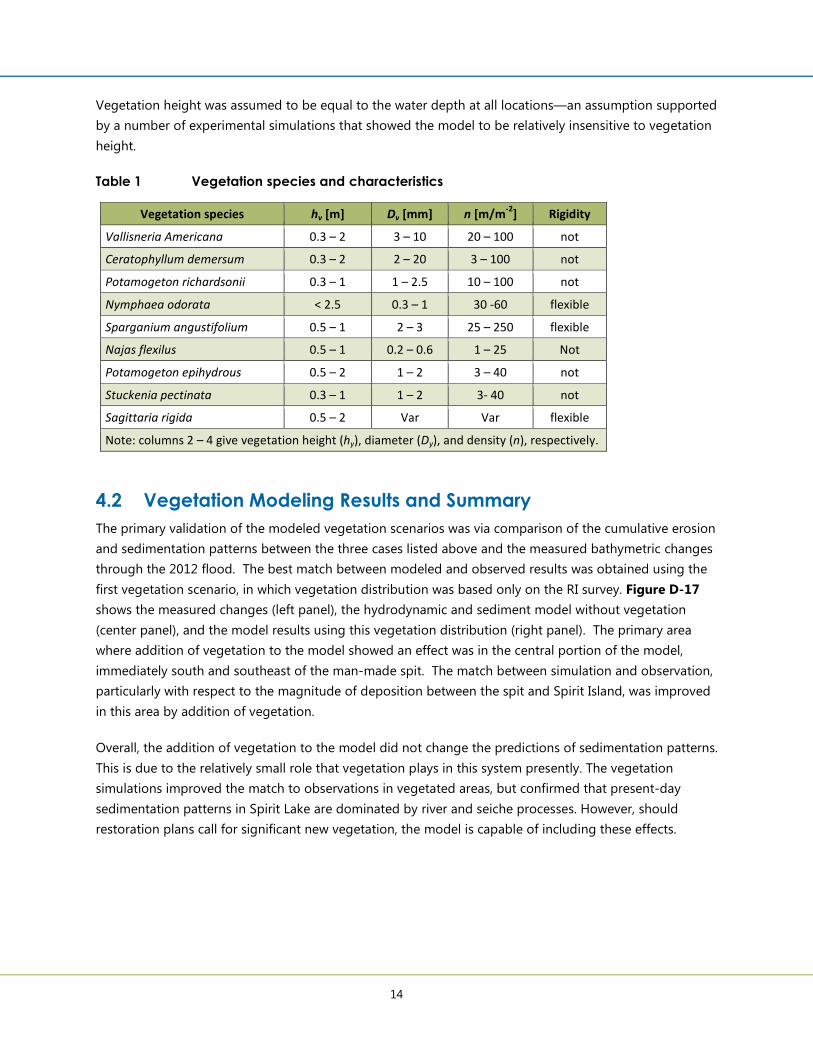
Estimates of vegetation height, density, size, and rigidity were required for implementation of vegetation
in Delft3D. A list of vegetation species present in Spirit Lake was developed as a component of the RI
(Table 1). The list included nine different species with various characteristics. As can be seen in Table 1, the
parameter range is generally quite large for individual species (particularly vegetation density), and often
larger than the range between different species. To assess the sensitivity of these various vegetation
characteristics, a range of stem density (n) values were used in the model (ranging between 0.1 –
10 m/m2).
The result of this vegetation sensitivity analysis was that the various species had an overall similar
morphological effect. Therefore, rather than assume particular values for each species to be distributed in
the model, one numerical vegetation type that combined average characteristics of all species was used.
14
Vegetation height was assumed to be equal to the water depth at all locations—an assumption supported
by a number of experimental simulations that showed the model to be relatively insensitive to vegetation
height.
Table 1 Vegetation species and characteristics
Vegetation species hv [m] Dv [mm] n [m/m-2
] Rigidity
Vallisneria Americana 0.3 – 2 3 – 10 20 – 100 not
Ceratophyllum demersum 0.3 – 2 2 – 20 3 – 100 not
Potamogeton richardsonii 0.3 – 1 1 – 2.5 10 – 100 not
Nymphaea odorata < 2.5 0.3 – 1 30 -60 flexible
Sparganium angustifolium 0.5 – 1 2 – 3 25 – 250 flexible
Najas flexilus 0.5 – 1 0.2 – 0.6 1 – 25 Not
Potamogeton epihydrous 0.5 – 2 1 – 2 3 – 40 not
Stuckenia pectinata 0.3 – 1 1 – 2 3- 40 not
Sagittaria rigida 0.5 – 2 Var Var flexible
Note: columns 2 – 4 give vegetation height (hy), diameter (Dy), and density (n), respectively.
4.2 Vegetation Modeling Results and Summary
The primary validation of the modeled vegetation scenarios was via comparison of the cumulative erosion
and sedimentation patterns between the three cases listed above and the measured bathymetric changes
through the 2012 flood. The best match between modeled and observed results was obtained using the
first vegetation scenario, in which vegetation distribution was based only on the RI survey. Figure D-17
shows the measured changes (left panel), the hydrodynamic and sediment model without vegetation
(center panel), and the model results using this vegetation distribution (right panel). The primary area
where addition of vegetation to the model showed an effect was in the central portion of the model,
immediately south and southeast of the man-made spit. The match between simulation and observation,
particularly with respect to the magnitude of deposition between the spit and Spirit Island, was improved
in this area by addition of vegetation.
Overall, the addition of vegetation to the model did not change the predictions of sedimentation patterns.
This is due to the relatively small role that vegetation plays in this system presently. The vegetation
simulations improved the match to observations in vegetated areas, but confirmed that present-day
sedimentation patterns in Spirit Lake are dominated by river and seiche processes. However, should
restoration plans call for significant new vegetation, the model is capable of including these effects.
15
5.0 Wave Modeling
Waves can lead to significant remobilization and transport of sediment in certain environments, and
therefore consideration of their potential effects in Spirit Lake was an important component of model
development. Waves can affect bed sediment by elevating near-bed shear stresses during their passage
along the water surface. Waves may also create currents (e.g.: “longshore” currents) potentially capable of
sediment transport. Data collected during the RI (Barr, 2013) illustrated that wave generated currents
were not important within Spirit Lake.
Wave heights within Spirit Lake were measured during both the 2011 and 2012 RI field campaigns.
Significant wave heights during these campaigns were found to be low typically, on the order of a few
centimeters (see Section 2). However, significant wave events have been observed during other site visits,
and the meteorological station documented periodic high wind events capable of generating larger
waves. Therefore the aim of the wave modeling was to quantify potential effects of more extreme waves
on bed stability and sediment redistribution, as well as wave interaction with river currents.
Three numerical approaches were used to evaluate the magnitude and potential effect of waves in Spirit
Lake, each of which are discussed in this Section:
1. Finite Depth Wind Wave Model: A simplistic numerical model used to create preliminary wind-
wave characteristics and to check outputs from other wave models.
2. SWAN (Simulating Waves Nearshore): A third-generation wave model which computes random,
short crested waves in coastal regions and inland waters.
3. XBeach: A 2-dimensional model for calculating wave propagation in shallow water near shore
environments.
5.1 Meteorological Conditions
Aside from bathymetry and basin geometry, wind characteristics are the key driver of wave formation.
Data from the Bong Airport was evaluated to develop a set of wind speed and direction data that would
represent strong to severe events to establish a design event. From these data four test cases were
developed (Table 2).
16
Table 2 Wind conditions used for wave modeling. Wind direction is defined in the nautical
convention (north = 0 degrees, east = 90 degrees).
Case Wind Speed [m/s] Wind Origin [deg]
1 10 45
2 12 67.5
3 7 45
4 10 67.5
5.2 Finite Depth Wind Wave Model
Wave height in a shallow setting like Spirit Lake is limited by the depth of the water, as increasingly large
waves experience elevated drag on the bottom, and become unstable. The Finite Depth Wind Wave
Model (FDWWM; Kamphuis, 2010) was used to estimate the largest physically reasonable waves possible
for a given fetch length, wind speed, and depth. The output of this model provided validation and
corroboration for the more sophisticated modeling techniques presented below. The inputs used for this
modeling were a maximum fetch length for Spirit Lake of roughly 2.3 km in the NNE-SSW direction, and
an average water depth of 2 m. Wind speeds/directions are listed in Table 2.
Results of the model (Table 3) indicated characteristic wave heights of 0.2 – 0.4 m, with a wave period of
approximately 2 seconds. These are reasonable values based on site observational experience, and are
comparable to those found in other settings with relatively limited fetch length and shallow bathymetry,
like Spirit Lake. It is expected, as seen in data collected during the RI, that actual wave heights in the
study area would be smaller, due to wave refraction and shoaling. As waves propagate into shallow water
their wave lengths and wave heights change as the waves “feel” the bed, and these changes are referred
to as wave refraction and wave shoaling. In addition, vegetation and other natural debris within Spirit
Lake would act to dissipate wave energy—phenomena not included in the FDWWM. Given the
assumptions/simplifications described above, the results of the Finite Depth Wind Wave Model are
considered to be the upper limit for wave height and period in Spirit Lake.
Table 3 Results of finite depth wind wave model for all four cases
Case U [m/s] θθθθ [o] Hs [m] T [s]
1 & 4 10 45 0.34 2.0
2 12 67.5 0.42 2.2
3 7 45 0.23 1.7
Note: U, t, Hs, and T indicate wind speed, wind direction, predicted significant
wave height, and predicted wave period, respectively.
17
5.3 SWAN
5.3.1 Model Setup
The SWAN wave model is set up within the Delft3D modeling suite (Delft3D – Wave) and uses the same
computational grid as the flow model (see Figure D-8). This component of the wave modeling program
was used because the FDWWM discussed above only makes predictions for a particular fetch, water
depth, and wind speed. SWAN was used to model the entire wave field within Spirit Lake, including how
wave dynamics were affected by islands, shallow areas, and river currents.
For most applications SWAN does not need intensive calibration, and is considered robust for nearly all
applications (Deltares, 2013). However, for the modeling described herein, the expected wave
characteristics (height, length and period) are relatively small compared to typical SWAN applications.
Thus, certain wave model settings have been adjusted from their default values. These settings are
described in the following sub sections.
5.3.1.1 Bottom Friction
Default wave dissipation by bottom friction in SWAN is parameterized using the common formulation of
Hasselmann, et. al. (1973). Two different bottom friction coefficients are commonly applied with this
formulation: Swell type waves use a bottom friction coefficient of 0.038 m2s-3, and wind waves a bottom
friction of 0.067 m2s-3. Recent research, however, has shown that the value for wind waves might be too
high. Van Vledder, et. al. (2010) stated that the two characteristic values have been used for years despite
no theoretical foundation having been found for needing a distinction between wave types. It was found
that the value for swell waves worked well for both swell and wind type waves, and thus proposed 0.038
m2s-3 as a default bottom friction coefficient value. The Van Vledder, et. al. approach was used for the
Spirit Lake model.
5.3.1.2 Convergence Settings
A few numerical settings that influence iteration procedure had to be changed from the default
implementation of SWAN in Delft3D. Due to the relatively weak wave forcing in Spirit Lake (compared to
oceanic environments, for example), the numerical convergence criteria needed to be set more
restrictively. Setting the convergence criteria to a stricter value involved longer computation times, but
resulted in more accurate prediction, as the difference between the wave height and period in two
consecutive iteration steps was smaller. The default setting for relative change in wave height and period
between two consecutive iteration steps is 0.02 (expressed as a fraction of the predicted quantity, such as
significant wave height). However, for this model it was set to 0.01. Thus, a value of 0.01 required that the
difference between the calculated values for successive numerical iterations must be less than 1% of the
mean value of all computed values. For most SWAN applications these settings are not very important.
However, for low-energy wave conditions (like those in Spirit Lake), stricter convergence criteria are
critical.
For similar reasons, the percentage of the wet grid cells where the above criteria was required to be met
was increased from a default of 98% to a stricter value of 99%.
18
5.3.1.3 Frequency Domain Settings
Due to the relatively small wave periods expected in Spirit Lake (Table 3), the default SWAN frequency
domain needed to be modified. High frequency waves are more common in Spirit Lake than in more
typical SWAN applications. Therefore the maximum frequency was increased to 2.5 Hz (from a default of
1 Hz), thus including waves with a period as short as 0.4 seconds (as opposed to the default of 1 second).
In addition, relatively long waves cannot form in Spirit Lake, so the minimum frequency was increased
from the default value of 0.05 Hz to 0.1 Hz. This restricted the wave periods modeled to less than 10
seconds instead of 20 seconds. The number of frequency bins was also increased to better discretize the
expected wave frequency range.
5.3.2 SWAN Model Results
The SWAN simulations were run to represent simplistic extreme wind condition cases, so as to develop an
understanding of the maximum potential wave conditions that are possible in Spirit Lake. Coupling the
low flow hydrodynamics with SWAN produced a 2-month long modeling period, which is much longer
than any one sustained wind pattern observed in the meteorological record. However, this simulation
provided ample time for full development of the wave field when a single wind speed from a single
direction was applied for the length of the model. In addition to allowing waves to fully develop, the long
run period also allowed for wave conditions to be modeled over changing water levels, which can have an
effect on wave conditions. For the modeling time period, the water level varied from +0.3 to -0.3 meters
relative to the mean water level.
The SWAN modeling results showed significant wave heights that vary from 0.1 to 0.3 meters, while the
period varies from 1 to 2 seconds. As expected, the largest wave heights were found associated with Case
2 wind speeds of 12 meters per second, a result comparable to the FDWWM results presented in Table 3.
Maps of important wave characteristics for Case 2 are given in Figure D-18. Local geometry and
bathymetry within Spirit Lake had a role in wave propagation; though nowhere did wave heights exceed
the maximum height of 0.42 meters predicted by the FDWMM (Table 3), due to generally shallower
depths than those used as input to the FDWWM.
The central result of the SWAN modeling was a spatial distribution of maximum wave heights, periods,
and propagation directions that were consistent with the physical bounds predicted by the FDWWM. The
SWAN results showed how the wave field in Spirit Lake was affected by both local bathymetry and the
overall geometry of the shoreline (e.g., Spirit Island, man-made spit, etc.). The results of the SWAN
modeling, however, were not directly applicable to prediction of nearshore wave phenomena. This is due
to the fact that SWAN, though a powerful spectral wave modeling tool, does not model individual waves.
Rather, the validated SWAN results are used in the following sub section as a boundary condition for a
nearshore wave model targeted at the region of interest.
5.4 XBeach Nearshore Wave Modeling
XBeach was used to assess the effects of individual waves on nearshore sediment stability and transport.
XBeach is an open source shoreline process model. Designed to simulate short term “storm type” wave
events, XBeach was developed to evaluate rapid shoreline change on short time scales using a particular
19
wave climate (in contrast to SWAN, which is targeted at large-scale wave field generation, and not at
individual wave dynamics). XBeach was designed to operate over time scales on the order of a few days,
which is comparable in duration to the strong wind/storm events that impact Spirit Lake. The output of
the SWAN model was used as input to XBeach.
5.4.1 Spirit Lake XBeach Model Setup
The XBeach model domain was adapted from the Delft3D model described above. Figure D-19 illustrates
the curvilinear grid that was created to focus on the nearshore areas of the Unnamed Creek and Wire Mill
Deltas. Both deltas were included into one domain so that the effects of landforms on wave propagation
and shoaling could be taken into account.
Wind-wave results from SWAN were applied as boundary conditions at the “seaward” (eastern) boundary.
In addition to this boundary condition, larger “storm” waves were applied at the boundary to simulate
potential worst-case scenarios. Inputs included initial water level elevation, wave height, wave length,
peak wave period, and average wave direction, as predicted by SWAN. The XBeach input parameters are
shown in Table 4.
Table 4 XBeach input values
Case Significant Wave Height [m] Wave Frequency [1/s] Wave Direction [deg]
1 0.3 0.3 90
2 0.25 0.3 45
3 0.3 0.3 45
4 0.25 0.3 90
For the analyses described in this section, XBeach was used to calculate the wave induced bottom shear
stresses. These shear stresses were then used to identify areas of potential sediment erosion.
5.4.2 XBeach Model Results
Results of the various XBeach model runs (Cases 1-4) showed that the waves propagating from offshore
Spirit Lake were significantly affected by shoaling across the shallow water depths in the nearshore area.
This shoaling limits the amount of wave energy that reaches the study area and ultimately the shoreline.
The highest wave induced bed shear stresses occurred very near the shoreline, in < 0.3 m water depths,
where breaking occurs. Figure D-20 shows the spatial distribution of wave related shear stresses for
Case 1. High shear stresses were restricted to the near shore regions, and were highest just north of the
Wire Mill outlet. Only in the shallowest water, less than 30 centimeters, did shear stresses exceed the
critical value for potential sediment disturbance (0.1 Pa).
The implication of the XBeach modeling results, as well as each of the models used to provide the
boundary conditions, is that sediments in the Project site are generally very stable under even relatively
extreme wind/wave conditions. The wind roses of Figure D-7 indicated that winds like those used as
input to the XBeach model (10 m/s) were exceeded less than 1% of the time over the 6-year

20
meteorological record. Thus, simulation of such winds as sustained over 2 months is extremely
conservative. During this conservatively extreme simulation bed shear stresses were large enough to
mobilize sediment only immediately adjacent to the shoreline in water less than 0.3 m deep.
21
6.0 Summary
This Appendix describes a linked series of models that were constructed, calibrated, and validated to
produce an evaluation tool that includes the physical processes most critical for the assessment of bed
stability in Spirit Lake. Results of this modeling effort compare well with observations of the system made
during the RI, and corroborate the conceptual site model developed from those observations and
published in the RI Report. In particular, the linked models reproduce the erosion and sedimentation
patterns observed through the flood of record on the lower St. Louis River, which indicates they are well
suited to evaluation of Project alternatives under extreme conditions.
Several important physical phenomena that operate in Spirit Lake are illustrated by the model results and
summarized in this section.
6.1 River and Seiche Currents
The largest potential for morphodynamic change (and thus sediment impact) occurs during large
flow/flood events. During these events the St. Louis River overtops the primary channel along the eastern
edge of the Spirit Lake and flow moves through the central portion of the lake. This flow path increases
bed shear stresses through the lake, and delivers more sediment throughout the site. During the 500-
year flood event of June 2012 flow through Spirit Lake deposited as much as one meter of new sediment
in some areas while removing bed sediment in other areas. The Project site was not affected by erosion
during this event, but significant new sediment deposition occurred. The model reproduced this effect.
During low flow periods, little to no morphodynamic changes occur. During low flows the St. Louis River
carries very little sediment load, and higher velocity river flow is concentrated in the main river channel
along the eastern shore of Spirit Lake. Seiche dynamics are the largest influence on flow patterns within
Spirit Lake during low river flow, due in part to the presence of the dredge channel that extends from the
downstream end of Spirit Lake into the lake. This channel acts to provide an easy conduit for flow during
the filling and draining of the lake associated with periodic seiche. During the falling period of a seiche,
increased water velocities and bed shear stresses occur in offshore areas near the dredged channel, but
velocities remain below the critical threshold for sediment movement.
6.2 Vegetation Effects
Vegetation affects flow patterns and velocities within Spirit Lake, and thus influences the distribution of
sediment accumulation and impact. Addition of vegetation to the hydrodynamic and sediment transport
model showed that river and seiche flow patterns dominate sedimentary patterns throughout most of
Spirit Lake, but that denser vegetation near the man-made spit leads to a reduction of sedimentation in
that area. Further, field observations coupled with this modeling indicated that high flow events are likely
to remove vegetation, resulting in deposition and erosion patterns that are governed by flow. The fact
that addition of vegetation to the model improved the match between prediction and observation only
modestly indicates that Spirit Lake was not particularly vegetated prior to the 2012 flood. At the very
least, vegetation was not exerting a major influence on flow patterns prior to the flood.

22
6.3 Wave Effects
Wave modeling indicated that even extreme wind conditions produced characteristic waves that were
incapable of impacting sediments throughout the vast majority of Spirit Lake. Evaluation of individual
waves using XBeach illustrated that in the Project site bed shear stresses remain negligible except for
where wave breaking occurs in 0.30 m of water or less. This is due to the elevated bed shear stresses that
accompany breaking waves. Field observations indicate that even in this swash zone sediments are
presently relatively stable with coarser bed sediments having created an armoring layer.
6.4 Application to Project Alternatives
The numerical models described in this document represent an important tool for evaluating potential
Project designs and strategies. Each of the important processes identified in the RI as potentially
disturbing impacted sediments are included in the models, and their modeled behavior compared well
with observations made during the RI. As project design advances, the models described in this document
will be useful for evaluating the potential effects of future extreme events, as well as for evaluating how
revegetation might affect flow patterns in Spirit Lake.
23
7.0 References
Baptist, M. J., 2005, Modelling floodplain biogeomorphology. Ph.D. thesis, ISBN 90-407-2582-9, 193 pp.,
Delft University of Technology, Faculty of Civil Engineering and Geosciences, Section Hydraulic
Engineering.
Barr, 2013. Sediment Remedial Investigation Report. Great Lakes Legacy Act Project - Spirit Lake Sediment
Site - Former U. S. Steel Duluth Works St. Louis River, Duluth, Minnesota. Prepared for U. S. Steel
and U.S. EPA Great Lakes National Program Office, March 2013.
Deltares, 2013. Delft3D-FLOW Users Manual, v. 4.02, Delft, the Netherlands.
Kamphuis, J., 2010. Introduction to Coastal Engineering and Management, Advanced Series on Ocean
Engineering: 30, Singapore, 2010.
Partheniades, E., 1965. Erosion and Deposition of Cohesive Soils, Journal of the Hydraulics Division, ASCE 91
(HY 1): 105–139. 79, 329, 569
Roelvink D, et. al., eds., 2010. XBeach Model Description and Manual.
Hasselmann, K., T. P. Barnett, E. Bouws, H. Carlson, D. E. Cartwright, K. Enke, J. Ewing, H. Gienapp, D. E.
Hasselmann, P. Kruseman, A. Meerburg, P. Müller, D. J. Olbers,K. Richter, W. Sell and H. Walden,
1973. Measurements of wind wave growth and swell decay during the Joint North Sea Wave Project
(JONSWAP), Deutsche Hydrographische Zeitschrift 8 (12). 44, 125, 127, 132.
van Vledder, G., Zijlema, M., and Holthuijsen, L., 2010. Revisiting the JONSWAP bottom friction formulation,
Proceedings Of The 32nd International Conference On Coastal Engineering,1(32).
Van Rijn, L.C., 2007. Unified View of Sediment Transport by Currents and Waves I: Initiation of Motion, Bed
Roughness, and Bed-Load Transport, Journal of Hydraulic Engineering 133 (6): 649–667. vi, 260,
261, 262, 263, 264, 267, 627
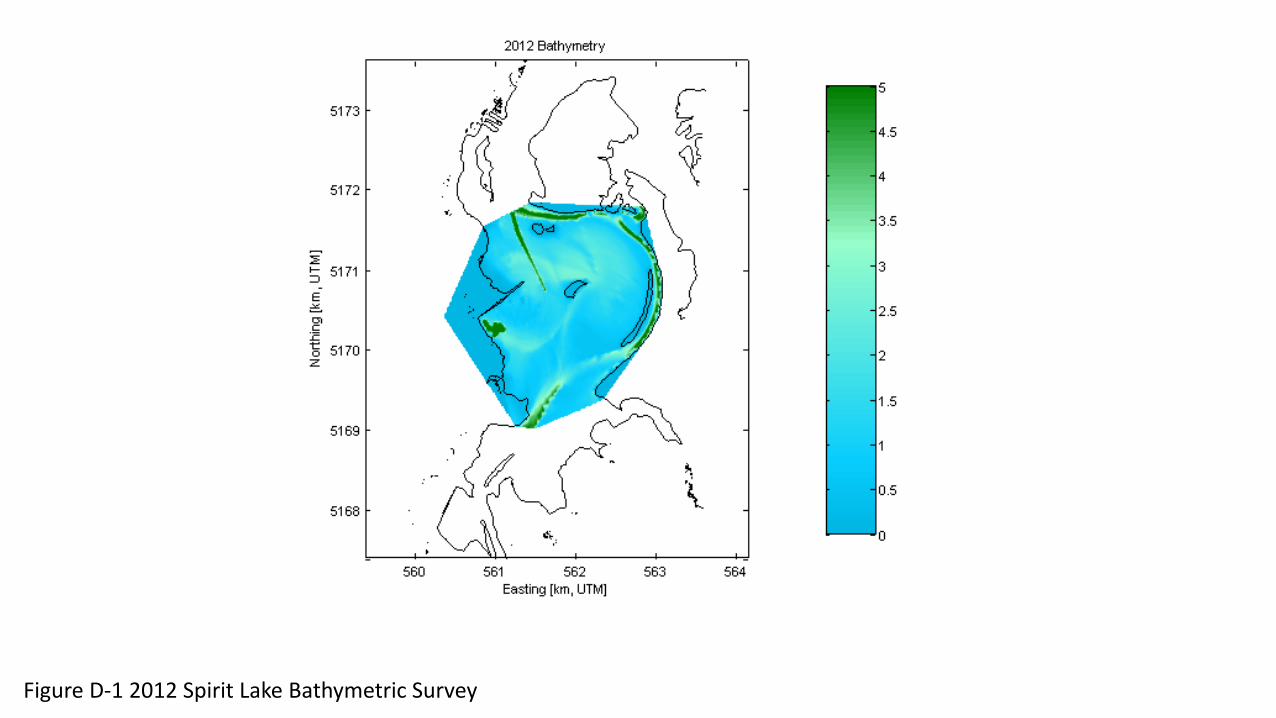
Figure D-1 2012 Spirit Lake Bathymetric Survey
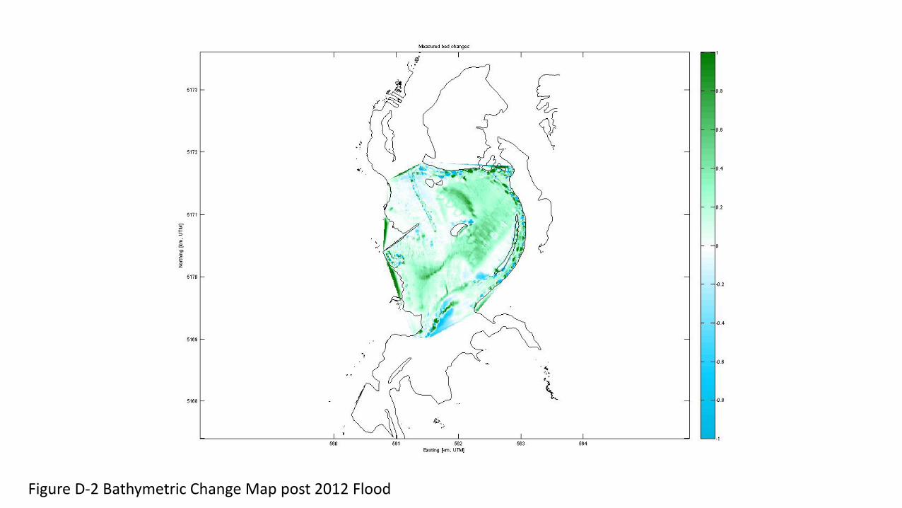
Figure D-2 Bathymetric Change Map post 2012 Flood
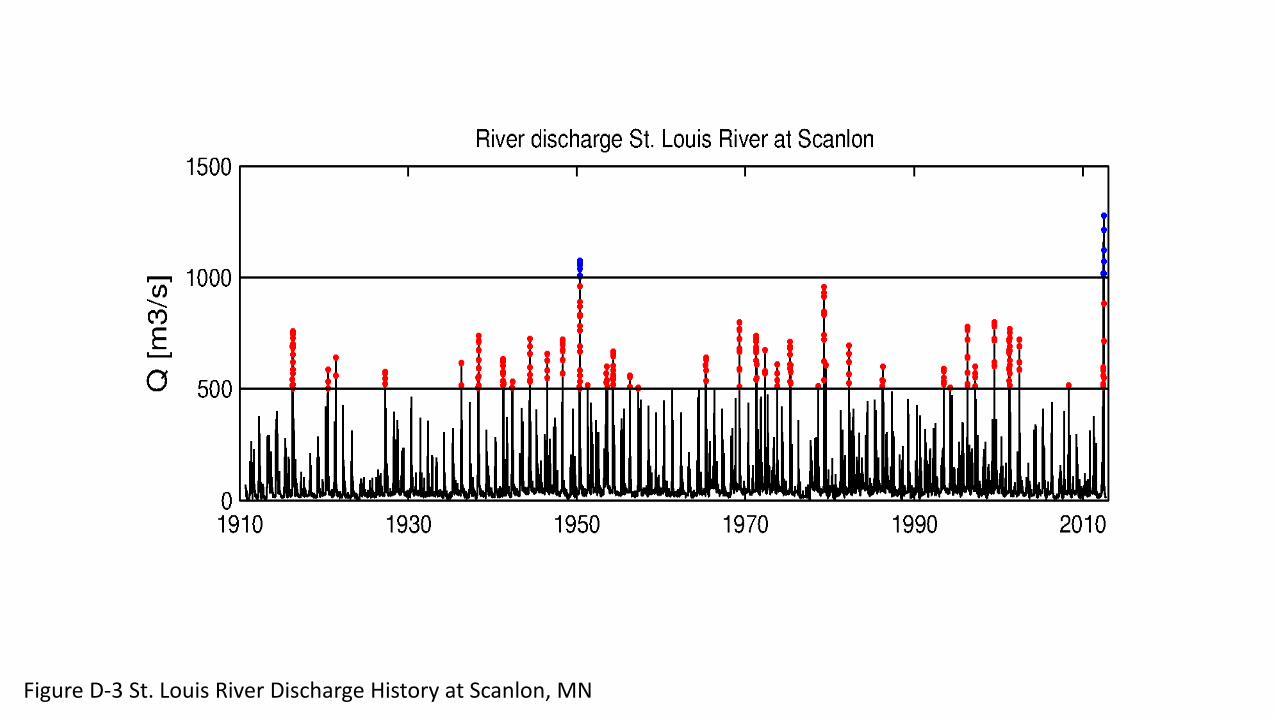
Figure D-3 St. Louis River Discharge History at Scanlon, MN
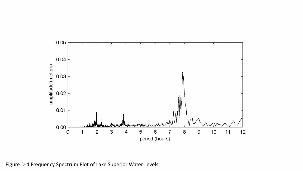
Figure D-4 Frequency Spectrum Plot of Lake Superior Water Levels
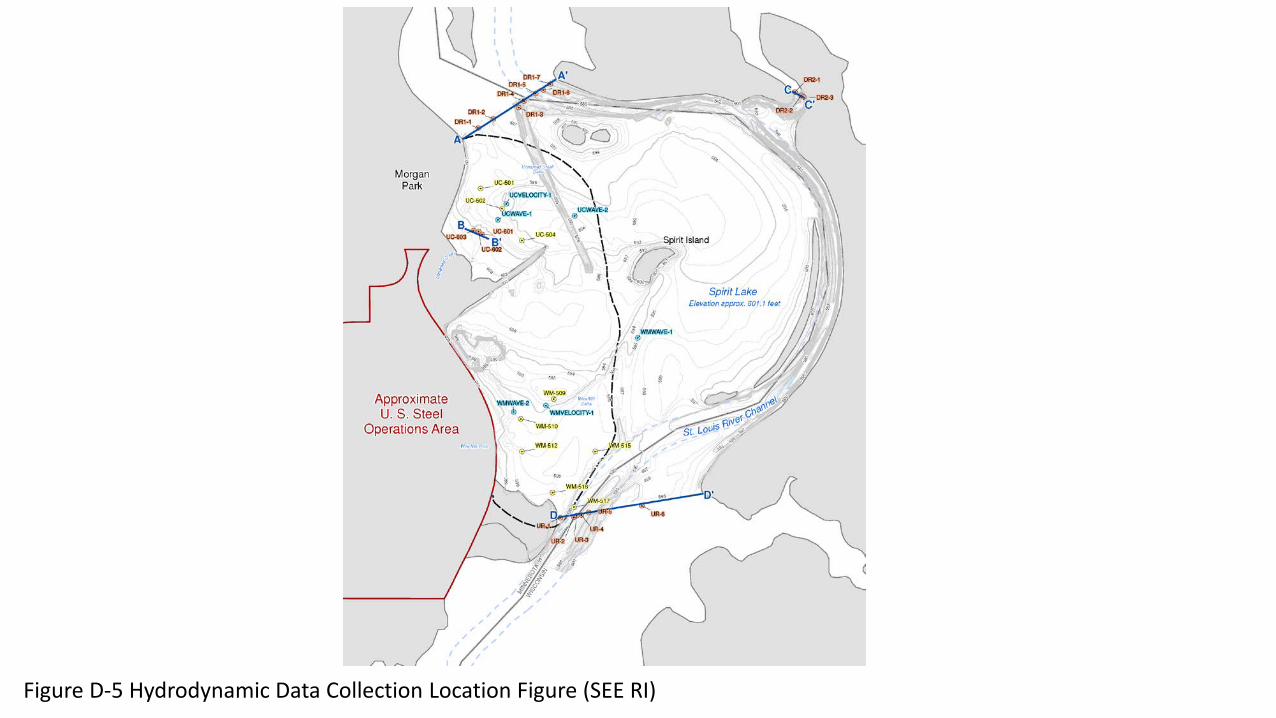
Figure D-5 Hydrodynamic Data Collection Location Figure (SEE RI)
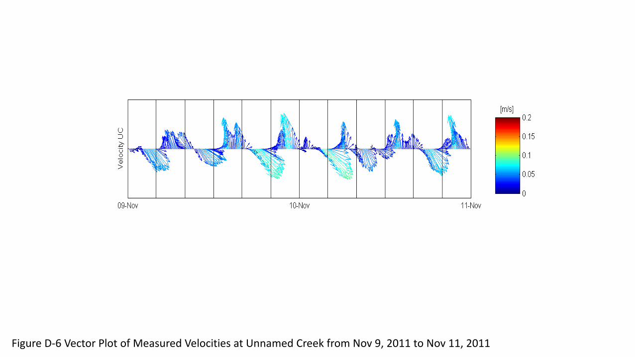
Figure D-6 Vector Plot of Measured Velocities at Unnamed Creek from Nov 9, 2011 to Nov 11, 2011
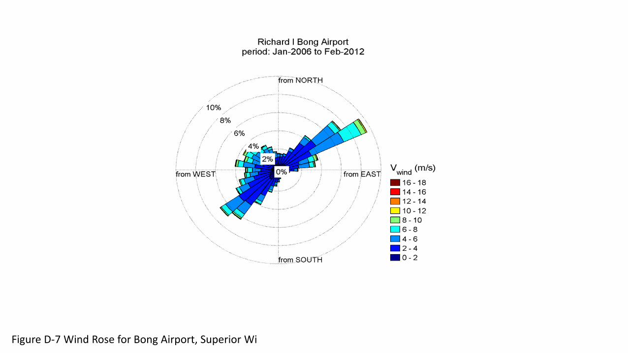
Figure D-7 Wind Rose for Bong Airport, Superior Wi
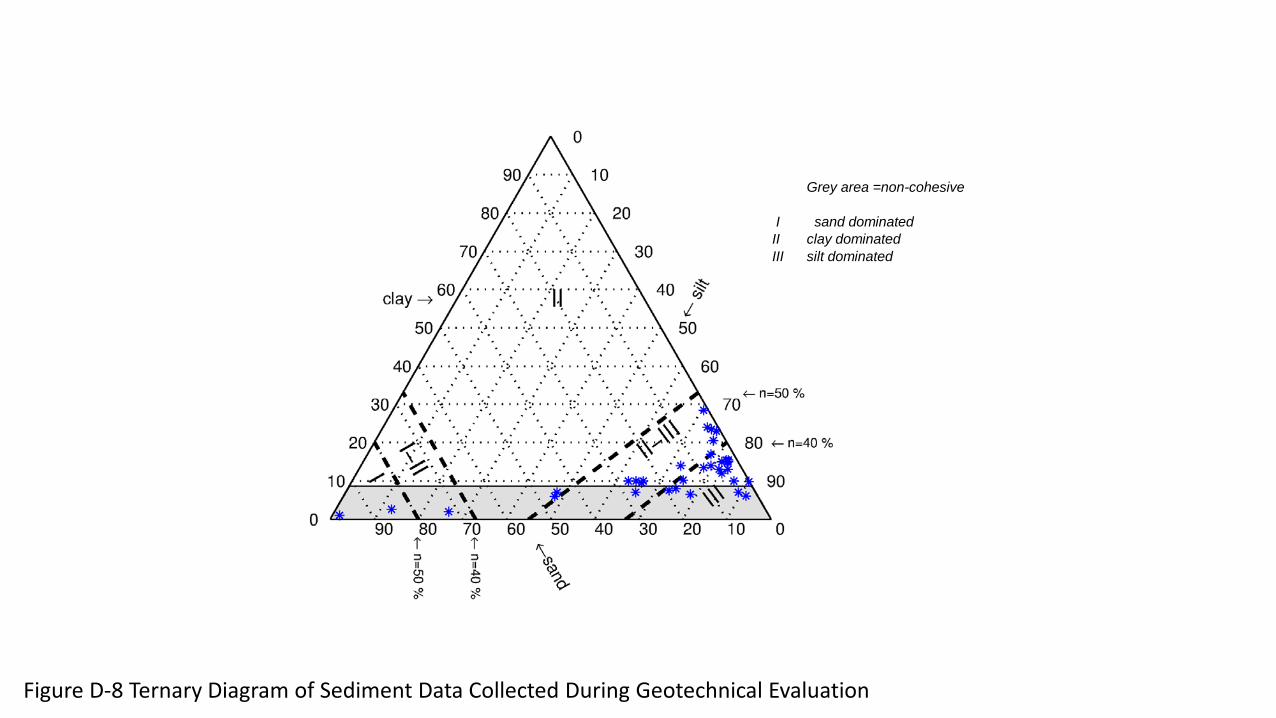
Figure D-8 Ternary Diagram of Sediment Data Collected During Geotechnical Evaluation
IIIIII
Grey area =non-cohesive
sand dominatedclay dominatedsilt dominated
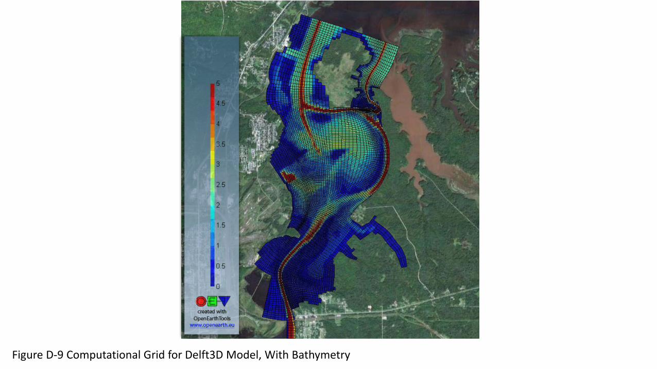
Figure D-9 Computational Grid for Delft3D Model, With Bathymetry
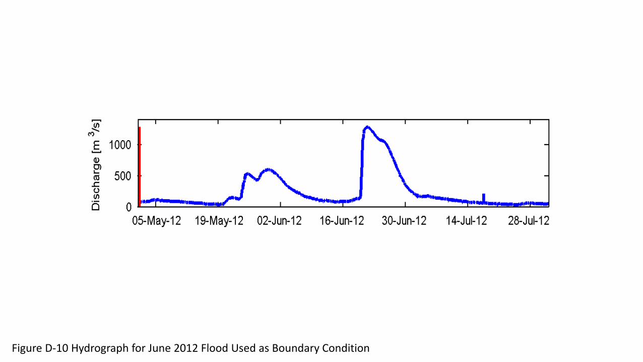
Figure D-10 Hydrograph for June 2012 Flood Used as Boundary Condition
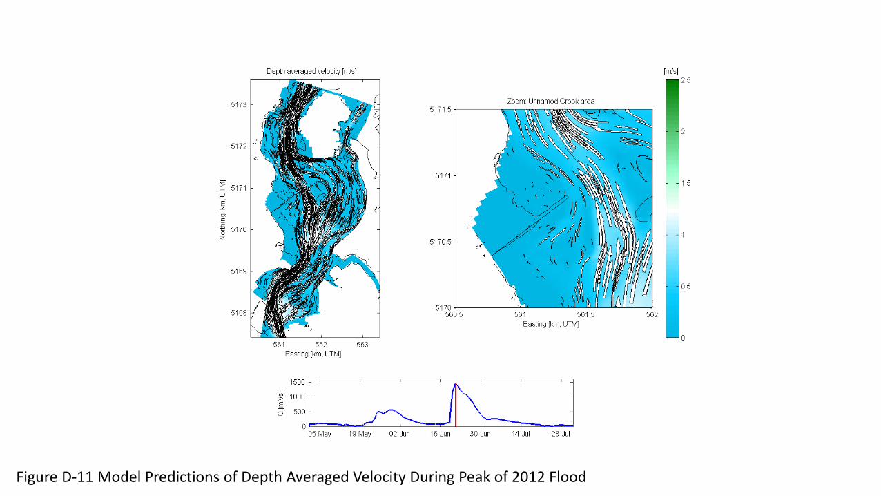
Figure D-11 Model Predictions of Depth Averaged Velocity During Peak of 2012 Flood
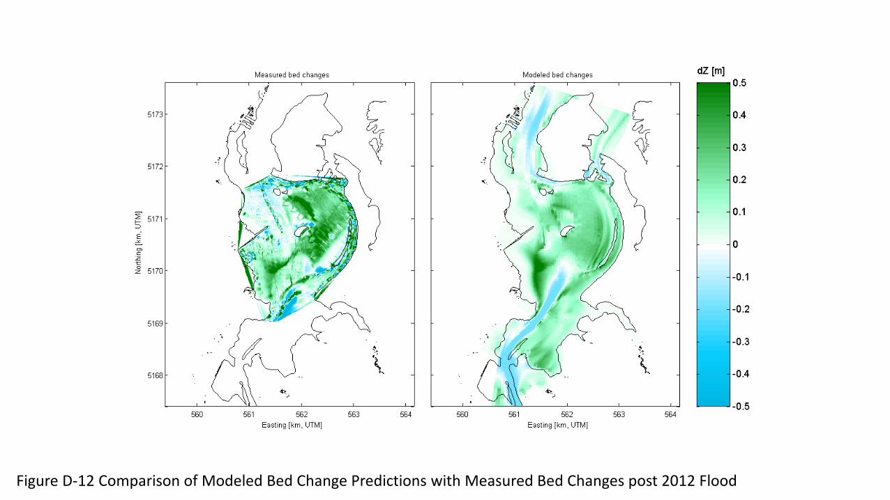
Figure D-12 Comparison of Modeled Bed Change Predictions with Measured Bed Changes post 2012 Flood
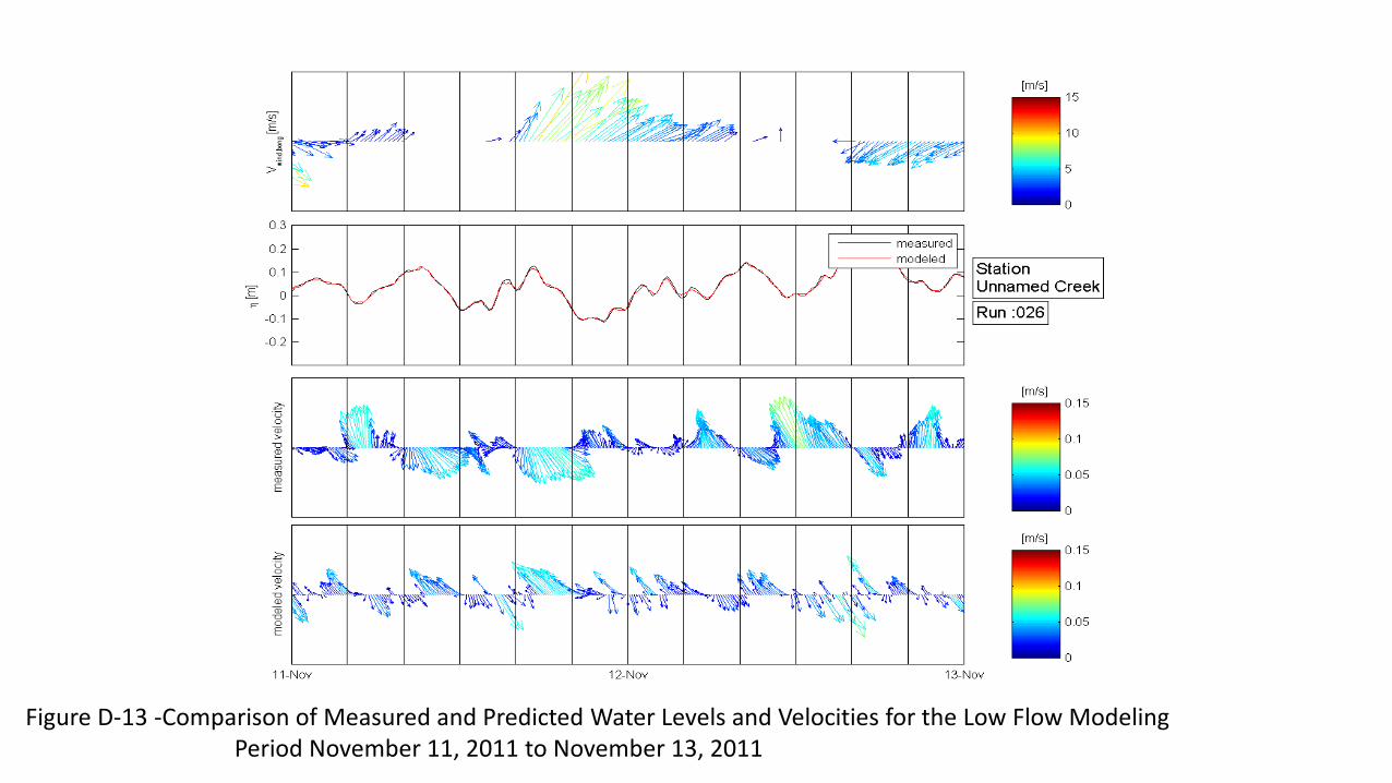
Figure D-13 -Comparison of Measured and Predicted Water Levels and Velocities for the Low Flow Modeling Period November 11, 2011 to November 13, 2011
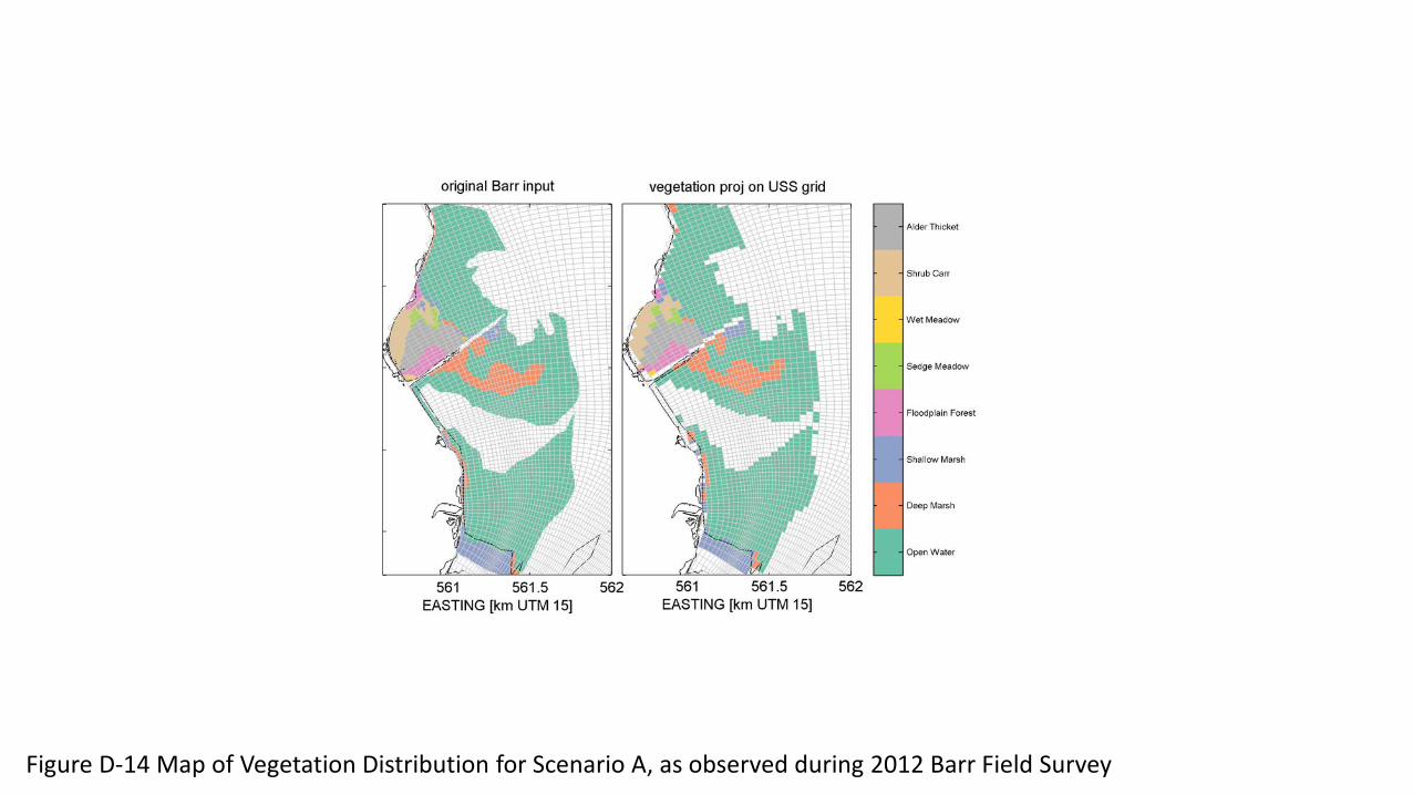
Figure D-14 Map of Vegetation Distribution for Scenario A, as observed during 2012 Barr Field Survey
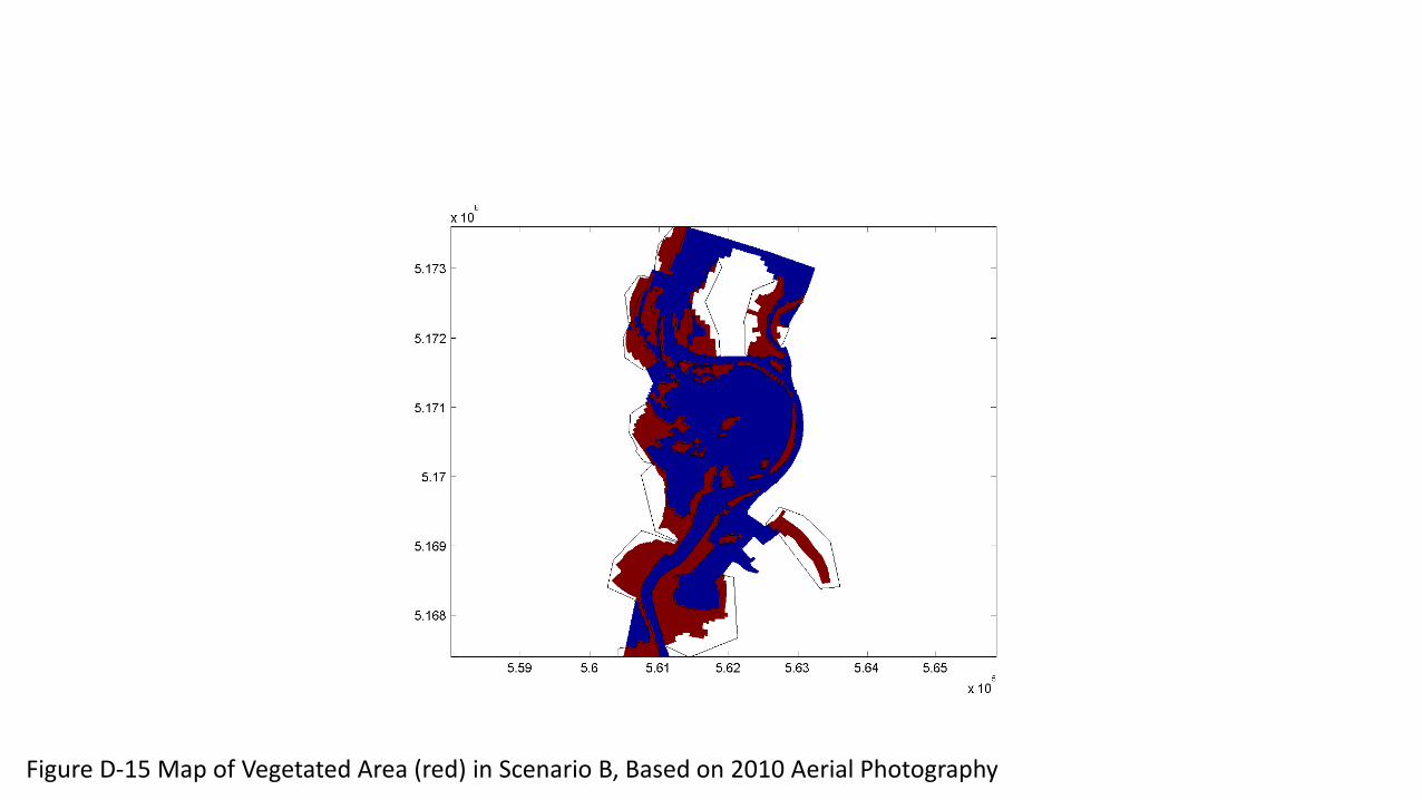
Figure D-15 Map of Vegetated Area (red) in Scenario B, Based on 2010 Aerial Photography
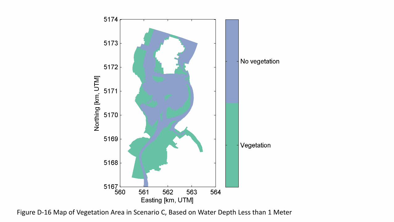
Figure D-16 Map of Vegetation Area in Scenario C, Based on Water Depth Less than 1 Meter
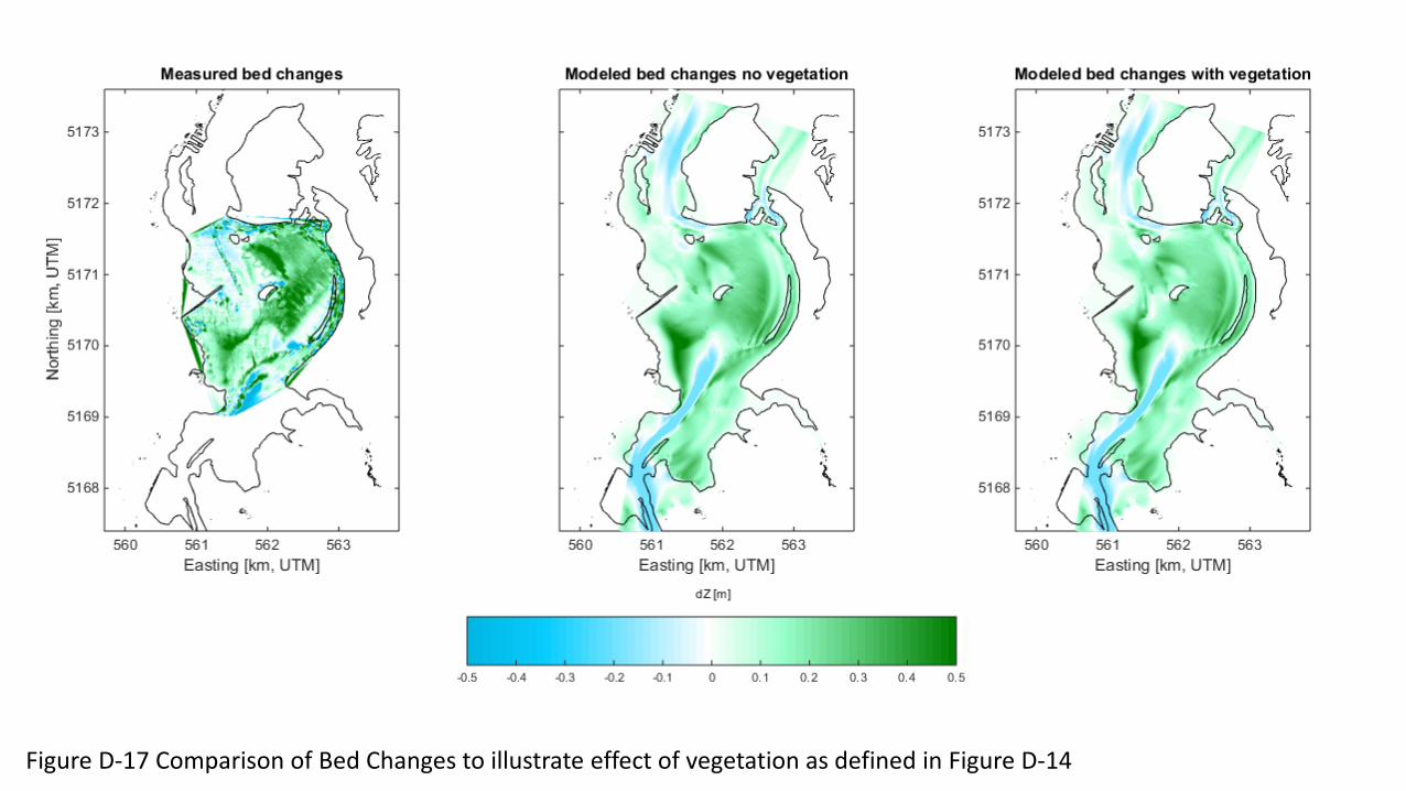
Figure D-17 Comparison of Bed Changes to illustrate effect of vegetation as defined in Figure D-14
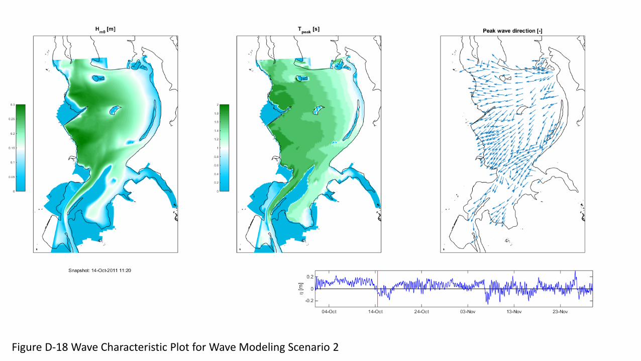
Figure D-18 Wave Characteristic Plot for Wave Modeling Scenario 2
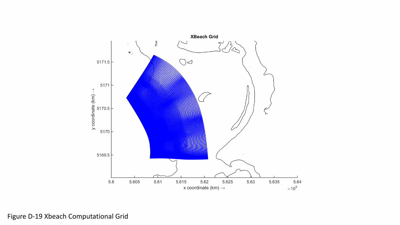
Figure D-19 Xbeach Computational Grid
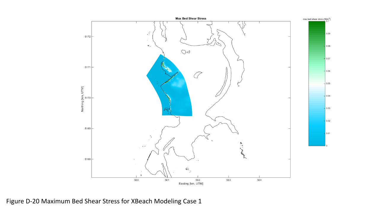
Figure D-20 Maximum Bed Shear Stress for XBeach Modeling Case 1