A stochastic modelling technique for predicting

Int. Journal of Applied Sciences and Engineering Research, Vol. 1, No. 2, 2012 www.ijaser.com

© 2012 by the authors – Licensee IJASER- Under Creative Commons License 3.0 [email protected]

Research article ISSN 2277 – 9442

�� 238

*Corresponding author (e-mail: [email protected])

Received on March, 2012; Accepted on March, 2012; Published on April, 2012

A stochastic modelling technique for predicting groundwater

table fluctuations with Time Series Analysis 1Sajal Kumar Adhikary,

2Md. Mahidur Rahman,

3Ashim Das Gupta

1- Assistant Professor, Department of Civil Engineering, Khulna University of Engineering &

Technology, Khulna-9203, Bangladesh

2- Junior Design Engineer, SARM Associates Limited, Dhaka-1213, Bangladesh

3- Professor Emeritus, Water Engineering and Management, Asian Institute of Technology (AIT),

Pathumthani-12120, Bangkok, Thailand

doi: 10.6088/ijaser.0020101024

Abstract: This paper demonstrates a methodology for modeling the groundwater table fluctuations

observed in a shallow unconfined aquifer of Bangladesh. For this purpose, Kushtia district of Bangladesh

has been selected as a case study area. A groundwater table monitoring well is selected in each upazilla

(sub-district) under the study area. The time series water table observations collected on a weekly basis

during the period from 1999 to 2006 from each well is used for experiments. Empirical result demonstrates

that observed data of groundwater level exhibits cyclic patterns and shows an annual periodicity. Box and

Jenkins univariate stochastic models widely known as ARIMA, are applied to simulate groundwater table

fluctuations in all monitoring wells under consideration in the study area. The predicted data using the best

models are compared to the observed time series and the resulting accuracy is checked using different error

parameters. The simulation revealed that ARIMA models generate reasonably accurate forecasts in terms

of numerical accuracy. The results also showed that the predicted data represent the actual data very well

for each monitoring well.

Key words: ARIMA model; groundwater table; periodogram; seasonality; stochastic modelling.

1. Introduction

Various quantitative analyses are required for complex and dynamic nature of water resources systems to

manage it properly. Groundwater table fluctuations over time in shallow aquifer systems need to be

evaluated for formulating or designing an appropriate groundwater development scheme. Models can be

simple images of things or can be complex, carrying all the characteristics of the object or process they

represent. A complex model will simulate the actions and reactions of the real thing. There has been

considerable research on modeling for various aspects of groundwater management strategy. The

conceptual and physically based models are the main tools for depicting hydrological variables and

understanding the physical processes that are taking place within a system (Anderson and Woessner, 1992).

There are varieties of techniques and methods available for analyzing the groundwater level fluctuation

through probability characteristics, time series methods, synthetic data generation, theory of runs, multiple

regression, group theory, pattern recognition and neural network methods. It is widely recognized that time

series modelling can be the better option for the area where nothing but the hydrological time series data is

in hand. A time series model is an empirical model for stochastically simulating and forecasting the

behaviour of uncertain hydrologic systems (Kim et al., 2005). However, it is very common that sufficient

hydrogeological parameters and domain boundary or initial conditions are often unavailable for physical

modelling. Most often, these parameters are very difficult to obtain as well because of the several natural

and anthropogenic factors (Kim et al., 2005). The stochastic time series models are the popular and useful

tools for medium-range forecasting and generating the synthetic data. A number of stochastic time series

A stochastic modelling technique for predicting groundwater table fluctuations with time series analysis

Sajal Kumar Adhikary, Md. Mahidur Rahman, Ashim Das Gupta

Int. Journal of Applied Sciences and Engineering Research, Vol. 1, No. 2, 2012

239

models such as the Markov, Box–Jenkins (BJ) Seasonal Autoregressive Integrated Moving Average

(ARIMA), deseasonalized Autoregressive Moving Average (ARMA), Periodic Autoregressive (PAR),

Transfer Function Noise (TFN) and Periodic Transfer Function Noise (PTFN), are in use for these

purposes (Brockwell and Davis, 2002; Box et al. 1994; Hipel and McLeod, 1994). The first three of these

are univariate models and the last two are multivariate models. In addition, the PAR and PTFN models are

periodic in nature (Mondal and Wasimi, 2007).

The selection of an appropriate method for modelling a particular problem depends on many factors,

such as the number of series to be modelled, required accuracy, modelling costs, ease of use of the models,

ease of interpretation of the results, etc. (Mondal and Wasimi, 2006). Several applications of all these

models have been proved to be very useful for analyzing groundwater level fluctuations over time in

several groundwater hydrology applications (Lee and Lee, 2000; Knotters and De Gooijer, 1999; Van Geer

and Zuur, 1997; Tankersley et al., 1993; Houston, 1983; Salas and Obeysekera, 1982). At the same time,

they have been widely applied to other relevant fields of science and engineering such as river flow

forecasting and synthetic data generation (Mondal and Wasimi, 2005; Mondal and Wasimi, 2003),

prediction of stream flow and water quality data (Kurunc et al., 2005), water resources monitoring and

assessment (Reghunath et al., 2005), simulation of drought periods (Yurekli et al., 2004) and traffic noise

time series data (Kumar and Jain, 1999). However, it is also reported in the literatures that when the

number of series to be modelled is relatively small and a large expenditure of time and effort can be

justified, BJ method (seasonal ARIMA) is generally preferable. The choice is due to its inclusion of a

family of models, which can be fitted to a wide variety of time series processes. An inherent advantage of

the seasonal ARIMA family of models is that few model parameters are required for describing time series,

which exhibit nonstationarity both within and across seasons (Mondal and Wasimi, 2006; Hipel and

McLeod, 1994). This paper attempts to develop seasonal ARIMA models as well as generalized equations

using the parameters of seasonal ARIMA models to show on of the modelling schemes regarding the

groundwater level fluctuations. It is expected that this study will provide useful information for developing

the appropriate strategy for managing the groundwater resources in the area under consideration.

2. The study area

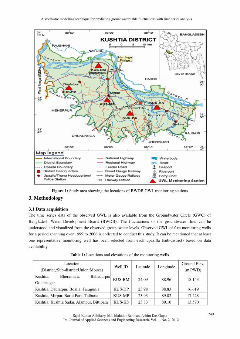
Kushtia district of Bangladesh has been selected as a case study area for this study (Figure 1) based on the

data availability of groundwater level (GWL) data. It covers an area of 1621 sq. km and is bounded by

Rajshahi, Natore and Pabna districts to the North, by Chuadanga and Jhenaidah districts to the South, by

Rajbari district to the east and by West Bengal and Meherpur district to the west. The upazillas (sub-district)

are Kushtia Sadar, Kumarkhali, Daulatpur, Mirpur, Bheramara and Khoksa. The Ganges, Gorai,

Mathabhanga, Kaligonga and Kumar are the main rivers flowing through the district. The average

maximum and minimum temperature is 37.8 0C and 11.2

0C, respectively with an annual average rainfall

of 1,467 mm. A larger portion of the Ganges-Kobadak irrigation project (also known as G-K project) of the

country is located in this district. During dry season, insufficient water supply from the Ganges River for

irrigation activities in the command area set a huge burden on the underground water reserves to satisfy the

ever-increasing demand. Therefore, the groundwater withdrawal rate is comparatively higher in the area

because of the growing demand for water due to intensive irrigation activities, along with the municipal

and commercial dependency on natural groundwater, and other relevant purposes.




240

Figure 1: Study area showing the locations of BWDB GWL monitoring stations

3. Methodology

3.1 Data acquisition

The time series data of the observed GWL is also available from the Groundwater Circle (GWC) of

Bangladesh Water Development Board (BWDB). The fluctuations of the groundwater flow can be

understood and visualized from the observed groundwater levels. Observed GWL of five monitoring wells

for a period spanning over 1999 to 2006 is collected to conduct this study. It can be mentioned that at least

one representative monitoring well has been selected from each upazilla (sub-district) based on data

availability.

Table 1: Locations and elevations of the monitoring wells

Location

(District,:Sub-district:Union:Mouza) Well ID Latitude Longitude

Ground Elev.

(m.PWD)

Kushtia, Bheramara, Bahadurpur,

Golapnagar KUS-BM 24.09 88.96 18.143

Kushtia, Daulatpur, Boalia, Taragunia KUS-DP 23.98 88.83 16.619

Kushtia, Mirpur, Barui Para, Talbaria KUS-MP 23.93 89.02 17.228

Kushtia, Kushtia Sadar, Alampur, Bittipara KUS-KS 23.83 89.10 13.570




241

Kushtia, Kumarkhali, Chapra, Jodu Boyra KUS-KK 23.84 89.20 12.960

The BWDB data is available on weekly basis with a unit of m.PWD. The m.PWD is the public works

datum (PWD) used by BWDB which is located at 0.46 m below the mean sea level (MSL) near

Bangladesh coast. For ease in identification, each monitoring well is given a unique name (e.g. KUS-DP)

using the first three characters from its located district (Kushtia) with additional two characters from its

located upazilla (e.g. Daulatpur) name. All the monitoring stations are positioned on the study area map in

the ArcGIS framework using their location (latitude and longitude) coordinates (Figure 1). Locations and

their ground elevations are shown in Table 1.

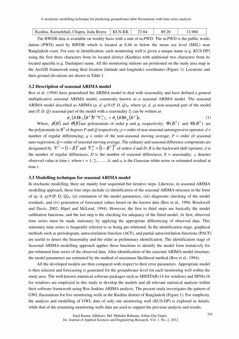
3.2 Description of seasonal ARIMA model

Box et al. (1994) have generalized the ARIMA model to deal with seasonality and have defined a general

multiplicative seasonal ARIMA model, commonly known as a seasonal ARIMA model. The seasonal

ARIMA model described as ARIMA (p, d, q)×(P, D, Q)S, where (p, d, q) non-seasonal part of the model

and (P, D, Q) seasonal part of the model with a seasonality S, can be written as

( ) ( ) ( ) ( ) t

S

Qqt

D

S

dS

Pp aBBzBB Θ=∇∇Φ θφ (1)

Where, ( )Bφ and ( )Bθ are polynomials of order p and q, respectively; )( SBΦ and )( SBΘ are

the polynomials in BS of degrees P and Q respectively; p = order of non-seasonal autoregressive operator; d =

number of regular differencing; q = order of the non-seasonal moving average; P = order of seasonal

auto-regression; Q = order of seasonal moving average. The ordinary and seasonal difference components are

designated by ( )dd B−=∇ 1 and ( )DSD

S B−=∇ 1 of orders d and D; B is the backward shift operator; d is

the number of regular differences; D is the number of seasonal differences; S = seasonality. zt denotes

observed value at time t, where t = 1, 2,………k; and at is the Gaussian white noise or estimated residual at

time t.

3.3 Modelling technique for seasonal ARIMA model

In stochastic modelling, there are mainly four sequential but iterative steps. Likewise, in seasonal ARIMA

modelling approach, these four steps include (i) identification of the seasonal ARIMA structure in the form

of (p, d, q)×(P, D, Q)S, (ii) estimation of the model parameters, (iii) diagnostic checking of the model

residuals, and (iv) generation of forecasted values based on the known data (Box et al., 1994; Brockwell

and Davis, 2002; Hipel and McLeod, 1994). However, the first to third steps are basically the model

calibration functions, and the last step is the checking for adequacy of the fitted model. At first, observed

time series must be made stationary by applying the appropriate differencing of observed data. This

stationary time series is frequently referred to as being pre-whitened. In the identification stage, graphical

methods such as periodogram, autocorrelation function (ACF), and partial autocorrelation functions (PACF)

are useful to detect the Seasonality and the order as preliminary identification. The identification stage of

Seasonal ARIMA modelling approach applies these functions to identify the model form tentatively for

pre-whitened time series of the observed data. After identification of the seasonal ARIMA model structure,

the model parameters are estimated by the method of maximum likelihood method (Box et al., 1994).

All the developed models are then compared with respect to their error parameters. Appropriate model

is then selected and forecasting is generated for the groundwater level for each monitoring well within the

study area. The well-known statistical software packages such as MINITABv14 for windows and SPSSv16

for windows are employed in this study to develop the models and all relevant statistical analysis within

their software framework using Box-Jenkins ARIMA analysis. The present study investigates the pattern of

GWL fluctuations for five monitoring wells in the Kushtia district of Bangladesh (Figure 1). For simplicity,

the analysis and modelling of GWL data of only one monitoring well (KUS-DP) is explored in details,

while that of the remaining monitoring wells data are used to support the previous analysis and results.




242

4. Results and discussions

4.1 Identification of ARIMA model structure

The first step in developing a Box-Jenkins time series model is to checking of the stationarity and presence

or absence of Seasonality in the observed time series data that needs to be modelled (Box et al., 1994). For

model identification, regression and periodic analyses were carried out to find the stationary time series

and periodicity or seasonal components of the observed data (Table 2).

4.1.1 Regression analysis

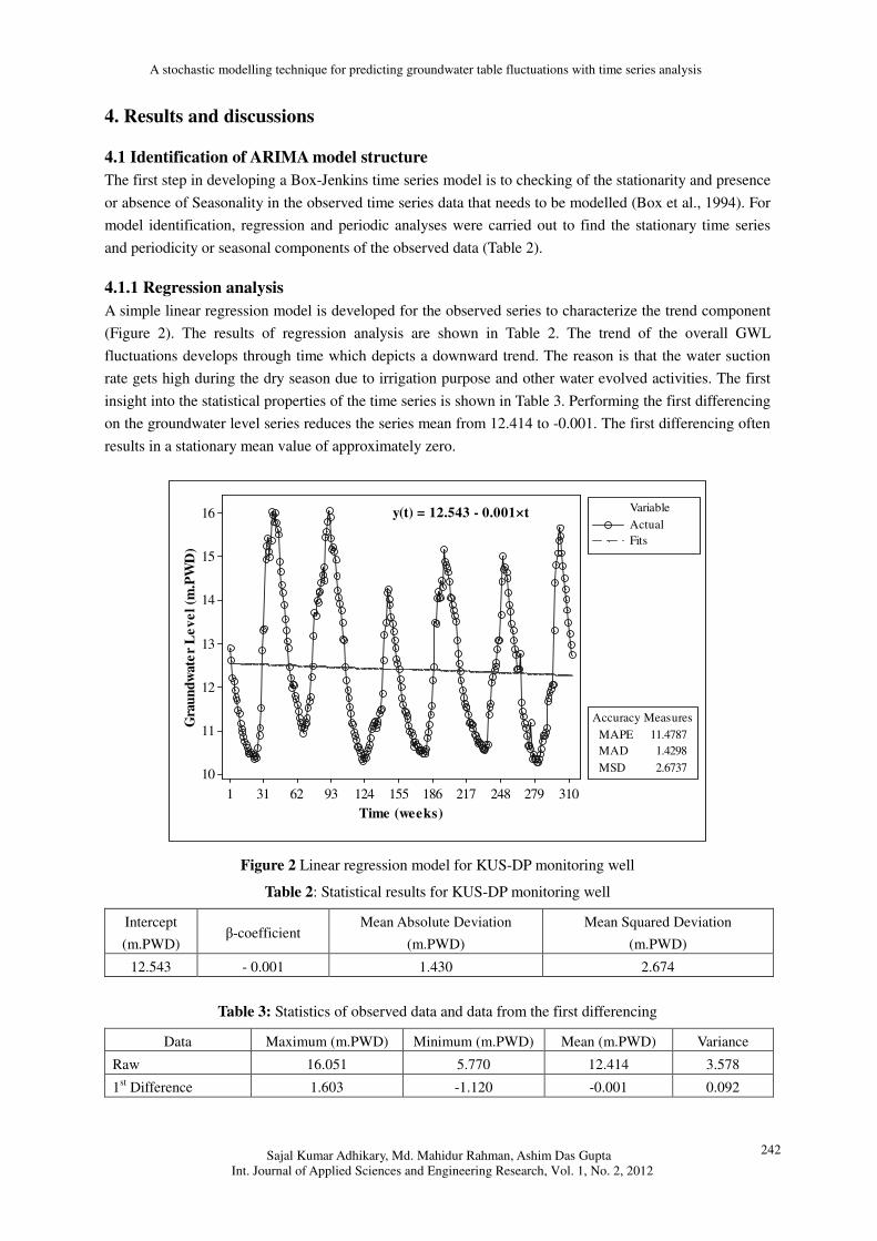
A simple linear regression model is developed for the observed series to characterize the trend component

(Figure 2). The results of regression analysis are shown in Table 2. The trend of the overall GWL

fluctuations develops through time which depicts a downward trend. The reason is that the water suction

rate gets high during the dry season due to irrigation purpose and other water evolved activities. The first

insight into the statistical properties of the time series is shown in Table 3. Performing the first differencing

on the groundwater level series reduces the series mean from 12.414 to -0.001. The first differencing often

results in a stationary mean value of approximately zero.

Time (weeks)

Gra

un

dw

ate

r L

ev

el

(m.P

WD

)

3102792482171861551249362311

16

15

14

13

12

11

10

Accuracy Measures

MAPE 11.4787

MAD 1.4298

MSD 2.6737

Variable

Actual

Fits

y(t) = 12.543 - 0.001×t

Figure 2 Linear regression model for KUS-DP monitoring well

Table 2: Statistical results for KUS-DP monitoring well

Intercept

(m.PWD) β-coefficient

Mean Absolute Deviation

(m.PWD)

Mean Squared Deviation

(m.PWD)

12.543 - 0.001 1.430 2.674

Table 3: Statistics of observed data and data from the first differencing

Data Maximum (m.PWD) Minimum (m.PWD) Mean (m.PWD) Variance

Raw 16.051 5.770 12.414 3.578

1st Difference 1.603 -1.120 -0.001 0.092




243

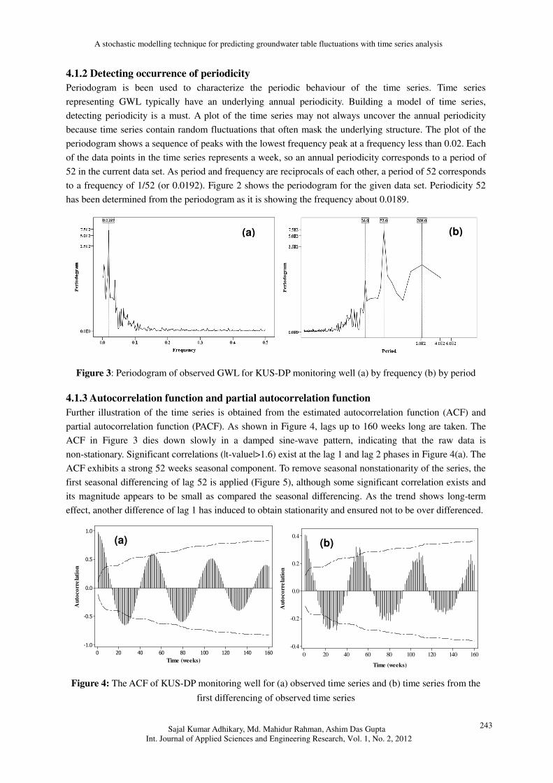
4.1.2 Detecting occurrence of periodicity

Periodogram is been used to characterize the periodic behaviour of the time series. Time series

representing GWL typically have an underlying annual periodicity. Building a model of time series,

detecting periodicity is a must. A plot of the time series may not always uncover the annual periodicity

because time series contain random fluctuations that often mask the underlying structure. The plot of the

periodogram shows a sequence of peaks with the lowest frequency peak at a frequency less than 0.02. Each

of the data points in the time series represents a week, so an annual periodicity corresponds to a period of

52 in the current data set. As period and frequency are reciprocals of each other, a period of 52 corresponds

to a frequency of 1/52 (or 0.0192). Figure 2 shows the periodogram for the given data set. Periodicity 52

has been determined from the periodogram as it is showing the frequency about 0.0189.

Figure 3: Periodogram of observed GWL for KUS-DP monitoring well (a) by frequency (b) by period

4.1.3 Autocorrelation function and partial autocorrelation function

Further illustration of the time series is obtained from the estimated autocorrelation function (ACF) and

partial autocorrelation function (PACF). As shown in Figure 4, lags up to 160 weeks long are taken. The

ACF in Figure 3 dies down slowly in a damped sine-wave pattern, indicating that the raw data is

non-stationary. Significant correlations (|t-value|>1.6) exist at the lag 1 and lag 2 phases in Figure 4(a). The

ACF exhibits a strong 52 weeks seasonal component. To remove seasonal nonstationarity of the series, the

first seasonal differencing of lag 52 is applied (Figure 5), although some significant correlation exists and

its magnitude appears to be small as compared the seasonal differencing. As the trend shows long-term

effect, another difference of lag 1 has induced to obtain stationarity and ensured not to be over differenced.

Figure 4: The ACF of KUS-DP monitoring well for (a) observed time series and (b) time series from the

first differencing of observed time series

Time (weeks)

Au

toco

rre

lati

on

160140120100806040200

1.0

0.5

0.0

-0.5

-1.0

Time (weeks)

Au

toco

rre

lati

on

160140120100806040200

0.4

0.2

0.0

-0.2

-0.4

(a) (b)

(a) (b)




244

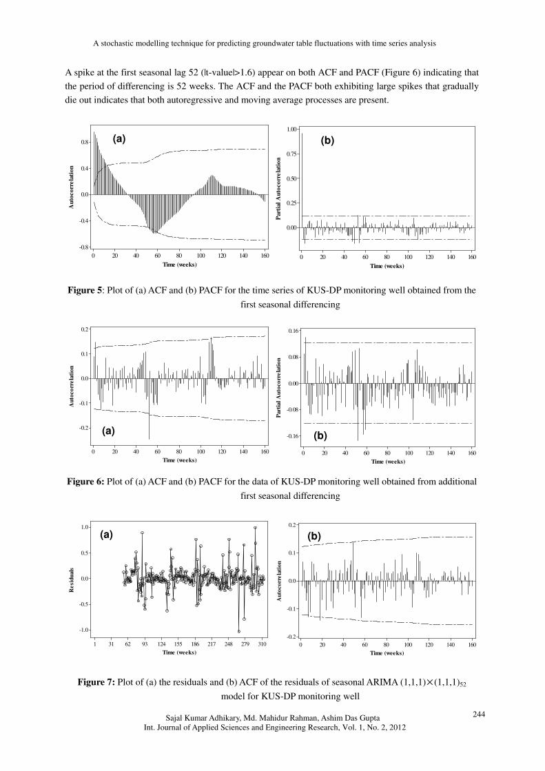
A spike at the first seasonal lag 52 (|t-value|>1.6) appear on both ACF and PACF (Figure 6) indicating that

the period of differencing is 52 weeks. The ACF and the PACF both exhibiting large spikes that gradually

die out indicates that both autoregressive and moving average processes are present.

Figure 5: Plot of (a) ACF and (b) PACF for the time series of KUS-DP monitoring well obtained from the

first seasonal differencing

Figure 6: Plot of (a) ACF and (b) PACF for the data of KUS-DP monitoring well obtained from additional

first seasonal differencing

Figure 7: Plot of (a) the residuals and (b) ACF of the residuals of seasonal ARIMA (1,1,1)× (1,1,1)52

model for KUS-DP monitoring well

Time (weeks)

Au

toco

rre

lati

on

160140120100806040200

0.8

0.4

0.0

-0.4

-0.8

Time (weeks)

Part

ial

Au

toco

rre

lati

on

160140120100806040200

1.00

0.75

0.50

0.25

0.00

(a) (b)

Time (weeks)

Au

toco

rre

lati

on

160140120100806040200

0.2

0.1

0.0

-0.1

-0.2

Time (weeks)

Part

ial

Au

toco

rre

lati

on

160140120100806040200

0.16

0.08

0.00

-0.08

-0.16(a) (b)

Time (weeks)

Re

sid

uals

3102792482171861551249362311

1.0

0.5

0.0

-0.5

-1.0

Time (weeks)

Au

toco

rre

lati

on

160140120100806040200

0.2

0.1

0.0

-0.1

-0.2

(a) (b)




245

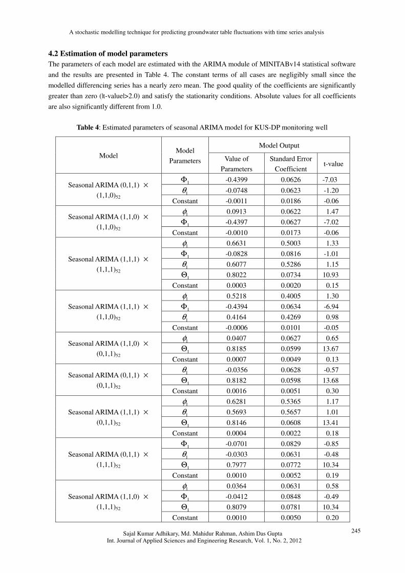
4.2 Estimation of model parameters

The parameters of each model are estimated with the ARIMA module of MINITABv14 statistical software

and the results are presented in Table 4. The constant terms of all cases are negligibly small since the

modelled differencing series has a nearly zero mean. The good quality of the coefficients are significantly

greater than zero (|t-value|>2.0) and satisfy the stationarity conditions. Absolute values for all coefficients

are also significantly different from 1.0.

Table 4: Estimated parameters of seasonal ARIMA model for KUS-DP monitoring well

Model Output

Model Model

Parameters Value of

Parameters

Standard Error

Coefficient t-value

1Φ -0.4399 0.0626 -7.03

1θ -0.0748 0.0623 -1.20 Seasonal ARIMA (0,1,1) ×

(1,1,0)52 Constant -0.0011 0.0186 -0.06

1φ 0.0913 0.0622 1.47

1Φ -0.4397 0.0627 -7.02 Seasonal ARIMA (1,1,0) ×

(1,1,0)52 Constant -0.0010 0.0173 -0.06

1φ 0.6631 0.5003 1.33

1Φ -0.0828 0.0816 -1.01

1θ 0.6077 0.5286 1.15

1Θ 0.8022 0.0734 10.93

Seasonal ARIMA (1,1,1) ×

(1,1,1)52

Constant 0.0003 0.0020 0.15

1φ 0.5218 0.4005 1.30

1Φ -0.4394 0.0634 -6.94

1θ 0.4164 0.4269 0.98


(1,1,0)52

Constant -0.0006 0.0101 -0.05

1φ 0.0407 0.0627 0.65

1Θ 0.8185 0.0599 13.67 Seasonal ARIMA (1,1,0) ×

(0,1,1)52 Constant 0.0007 0.0049 0.13

1θ -0.0356 0.0628 -0.57

1Θ 0.8182 0.0598 13.68 Seasonal ARIMA (0,1,1) ×

(0,1,1)52 Constant 0.0016 0.0051 0.30

1φ 0.6281 0.5365 1.17

1θ 0.5693 0.5657 1.01

1Θ 0.8146 0.0608 13.41


(0,1,1)52

Constant 0.0004 0.0022 0.18

1Φ -0.0701 0.0829 -0.85

1θ -0.0303 0.0631 -0.48

1Θ 0.7977 0.0772 10.34


(1,1,1)52

Constant 0.0010 0.0052 0.19

1φ 0.0364 0.0631 0.58

1Φ -0.0412 0.0848 -0.49

1Θ 0.8079 0.0781 10.34


(1,1,1)52

Constant 0.0010 0.0050 0.20




246

4.3 Model diagnostic checking

The statistical adequacy of the estimated models is then verified. The ACF function for the residuals

resulting from a good ARIMA model will have statistically zero autocorrelation coefficients. Figure 6

shows a plot of the residuals for Seasonal ARIMA (1,1,1) × (1,1,1)52 model. The residual plot shows

small variations around the zero mean. The plot of the estimated residuals and its ACF presented in Figure

7 indicates that there is no significant autocorrelation, and the model adopted will be acceptable.

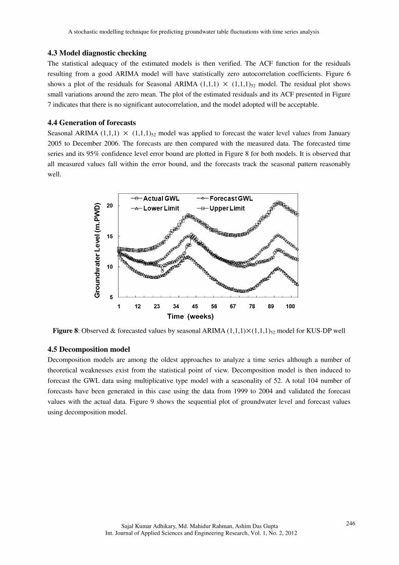
4.4 Generation of forecasts

Seasonal ARIMA (1,1,1) × (1,1,1)52 model was applied to forecast the water level values from January

2005 to December 2006. The forecasts are then compared with the measured data. The forecasted time

series and its 95% confidence level error bound are plotted in Figure 8 for both models. It is observed that

all measured values fall within the error bound, and the forecasts track the seasonal pattern reasonably

well.

Figure 8: Observed & forecasted values by seasonal ARIMA (1,1,1)× (1,1,1)52 model for KUS-DP well

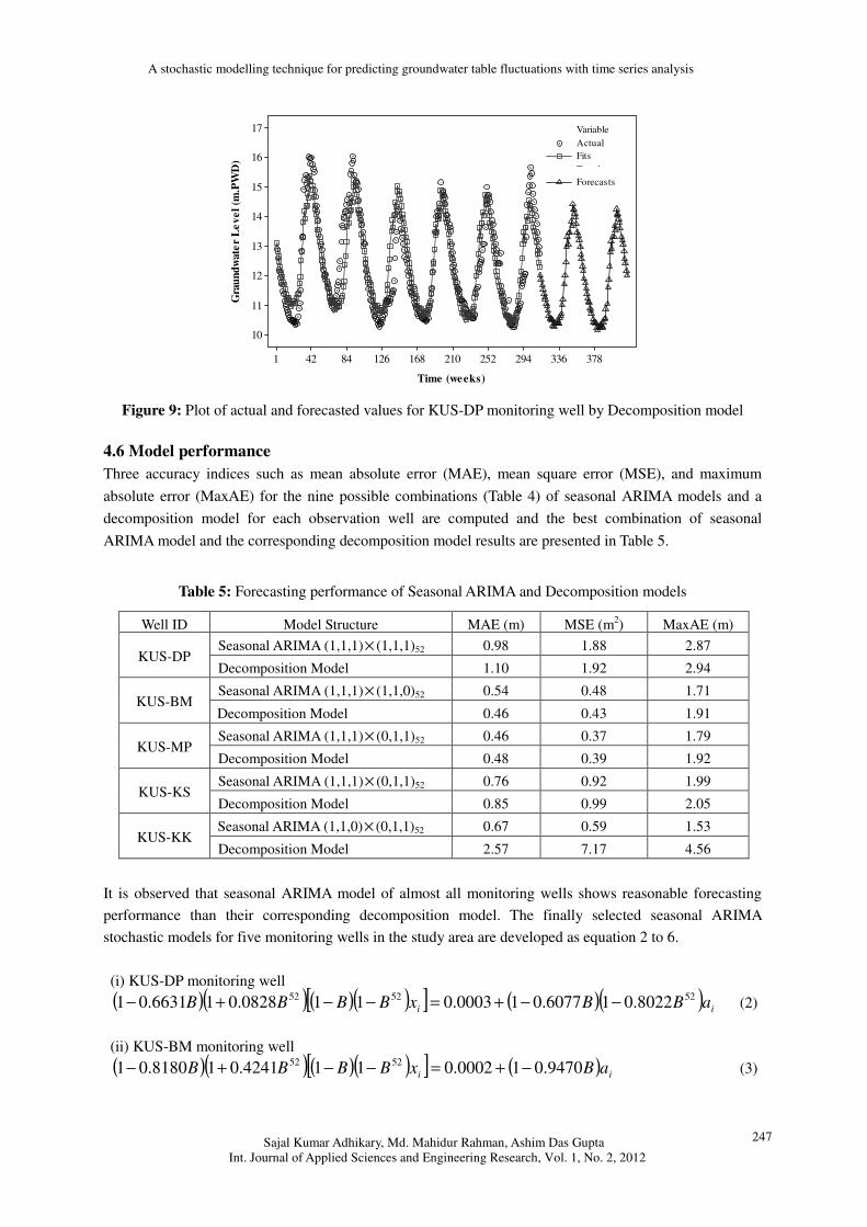
4.5 Decomposition model

Decomposition models are among the oldest approaches to analyze a time series although a number of

theoretical weaknesses exist from the statistical point of view. Decomposition model is then induced to

forecast the GWL data using multiplicative type model with a seasonality of 52. A total 104 number of

forecasts have been generated in this case using the data from 1999 to 2004 and validated the forecast

values with the actual data. Figure 9 shows the sequential plot of groundwater level and forecast values

using decomposition model.




247

Time (weeks)

Gra

un

dw

ate

r L

ev

el

(m.P

WD

)

37833629425221016812684421

17

16

15

14

13

12

11

10

Variable

Trend

Forecasts

Actual

Fits

Figure 9: Plot of actual and forecasted values for KUS-DP monitoring well by Decomposition model

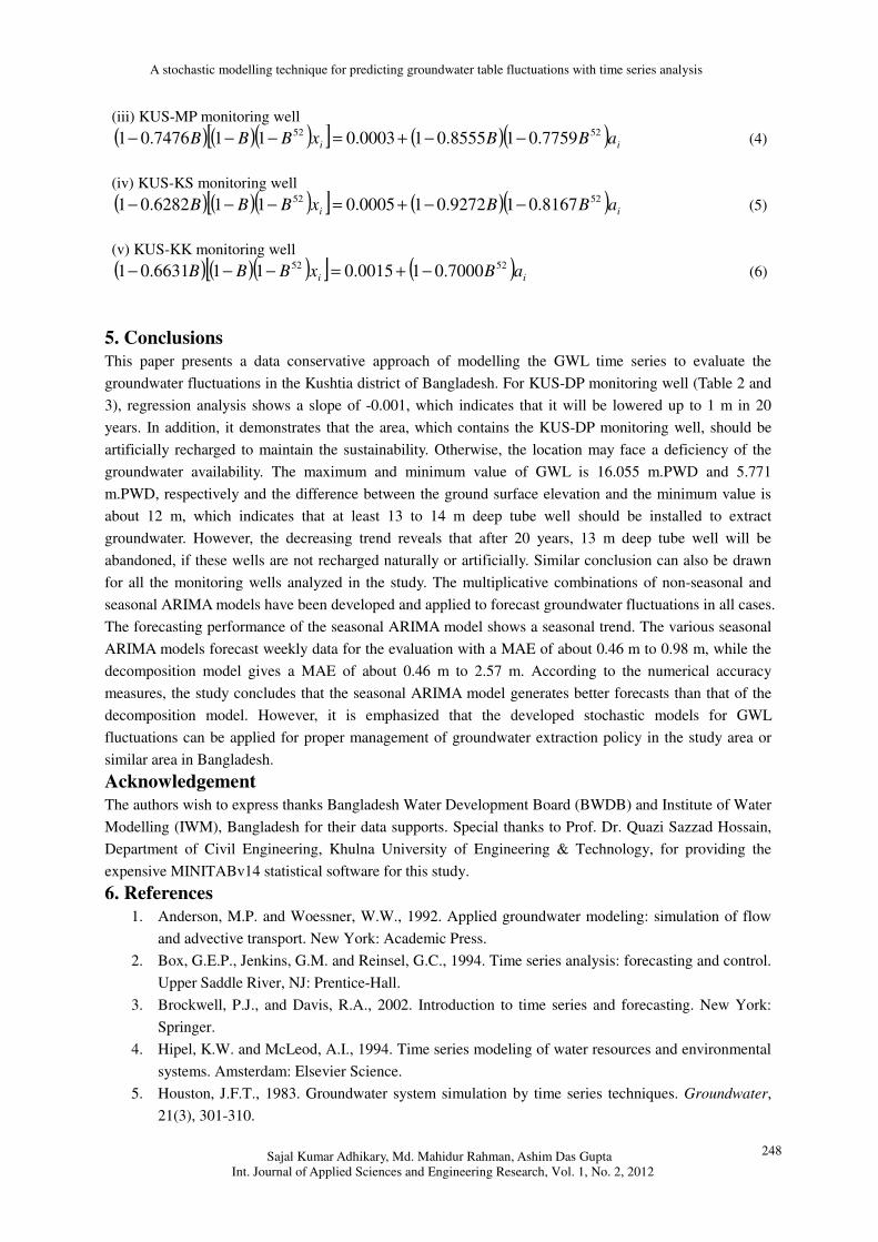
4.6 Model performance

Three accuracy indices such as mean absolute error (MAE), mean square error (MSE), and maximum

absolute error (MaxAE) for the nine possible combinations (Table 4) of seasonal ARIMA models and a

decomposition model for each observation well are computed and the best combination of seasonal

ARIMA model and the corresponding decomposition model results are presented in Table 5.

Table 5: Forecasting performance of Seasonal ARIMA and Decomposition models

Well ID Model Structure MAE (m) MSE (m2) MaxAE (m)

Seasonal ARIMA (1,1,1)× (1,1,1)52 0.98 1.88 2.87 KUS-DP

Decomposition Model 1.10 1.92 2.94

Seasonal ARIMA (1,1,1)× (1,1,0)52 0.54 0.48 1.71 KUS-BM


Seasonal ARIMA (1,1,1)× (0,1,1)52 0.46 0.37 1.79 KUS-MP


Seasonal ARIMA (1,1,1)× (0,1,1)52 0.76 0.92 1.99 KUS-KS


Seasonal ARIMA (1,1,0)× (0,1,1)52 0.67 0.59 1.53 KUS-KK


It is observed that seasonal ARIMA model of almost all monitoring wells shows reasonable forecasting

performance than their corresponding decomposition model. The finally selected seasonal ARIMA

stochastic models for five monitoring wells in the study area are developed as equation 2 to 6.

(i) KUS-DP monitoring well

( )( )( )( )[ ] ( )( )ii aBBxBBBB

525252 8022.016077.010003.0110828.016631.01 −−+=−−+− (2)

(ii) KUS-BM monitoring well

( )( ) ( )( )[ ] ( ) ii aBxBBBB 9470.010002.0114241.018180.01 5252 −+=−−+− (3)




248

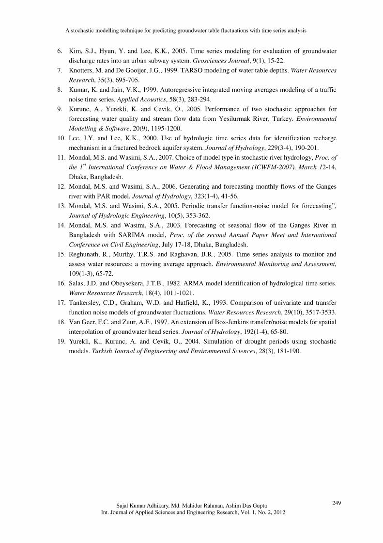
(iii) KUS-MP monitoring well

( ) ( )( )[ ] ( )( ) ii aBBxBBB5252 7759.018555.010003.0117476.01 −−+=−−− (4)

(iv) KUS-KS monitoring well

( ) ( )( )[ ] ( )( )ii aBBxBBB

5252 8167.019272.010005.0116282.01 −−+=−−− (5)

(v) KUS-KK monitoring well

( ) ( )( )[ ] ( )ii aBxBBB

5252 7000.010015.0116631.01 −+=−−− (6)

5. Conclusions

This paper presents a data conservative approach of modelling the GWL time series to evaluate the

groundwater fluctuations in the Kushtia district of Bangladesh. For KUS-DP monitoring well (Table 2 and

3), regression analysis shows a slope of -0.001, which indicates that it will be lowered up to 1 m in 20

years. In addition, it demonstrates that the area, which contains the KUS-DP monitoring well, should be

artificially recharged to maintain the sustainability. Otherwise, the location may face a deficiency of the

groundwater availability. The maximum and minimum value of GWL is 16.055 m.PWD and 5.771

m.PWD, respectively and the difference between the ground surface elevation and the minimum value is

about 12 m, which indicates that at least 13 to 14 m deep tube well should be installed to extract

groundwater. However, the decreasing trend reveals that after 20 years, 13 m deep tube well will be

abandoned, if these wells are not recharged naturally or artificially. Similar conclusion can also be drawn

for all the monitoring wells analyzed in the study. The multiplicative combinations of non-seasonal and

seasonal ARIMA models have been developed and applied to forecast groundwater fluctuations in all cases.

The forecasting performance of the seasonal ARIMA model shows a seasonal trend. The various seasonal

ARIMA models forecast weekly data for the evaluation with a MAE of about 0.46 m to 0.98 m, while the

decomposition model gives a MAE of about 0.46 m to 2.57 m. According to the numerical accuracy

measures, the study concludes that the seasonal ARIMA model generates better forecasts than that of the

decomposition model. However, it is emphasized that the developed stochastic models for GWL

fluctuations can be applied for proper management of groundwater extraction policy in the study area or

similar area in Bangladesh.

Acknowledgement

The authors wish to express thanks Bangladesh Water Development Board (BWDB) and Institute of Water

Modelling (IWM), Bangladesh for their data supports. Special thanks to Prof. Dr. Quazi Sazzad Hossain,

Department of Civil Engineering, Khulna University of Engineering & Technology, for providing the

expensive MINITABv14 statistical software for this study.

6. References

1. Anderson, M.P. and Woessner, W.W., 1992. Applied groundwater modeling: simulation of flow

and advective transport. New York: Academic Press.

2. Box, G.E.P., Jenkins, G.M. and Reinsel, G.C., 1994. Time series analysis: forecasting and control.

Upper Saddle River, NJ: Prentice-Hall.

3. Brockwell, P.J., and Davis, R.A., 2002. Introduction to time series and forecasting. New York:

Springer.

4. Hipel, K.W. and McLeod, A.I., 1994. Time series modeling of water resources and environmental

systems. Amsterdam: Elsevier Science.

5. Houston, J.F.T., 1983. Groundwater system simulation by time series techniques. Groundwater,

21(3), 301-310.




249

6. Kim, S.J., Hyun, Y. and Lee, K.K., 2005. Time series modeling for evaluation of groundwater

discharge rates into an urban subway system. Geosciences Journal, 9(1), 15-22.

7. Knotters, M. and De Gooijer, J.G., 1999. TARSO modeling of water table depths. Water Resources

Research, 35(3), 695-705.

8. Kumar, K. and Jain, V.K., 1999. Autoregressive integrated moving averages modeling of a traffic

noise time series. Applied Acoustics, 58(3), 283-294.

9. Kurunc, A., Yurekli, K. and Cevik, O., 2005. Performance of two stochastic approaches for

forecasting water quality and stream flow data from Yesilurmak River, Turkey. Environmental

Modelling & Software, 20(9), 1195-1200.

10. Lee, J.Y. and Lee, K.K., 2000. Use of hydrologic time series data for identification recharge

mechanism in a fractured bedrock aquifer system. Journal of Hydrology, 229(3-4), 190-201.

11. Mondal, M.S. and Wasimi, S.A., 2007. Choice of model type in stochastic river hydrology, Proc. of

the 1st International Conference on Water & Flood Management (ICWFM-2007), March 12-14,

Dhaka, Bangladesh.

12. Mondal, M.S. and Wasimi, S.A., 2006. Generating and forecasting monthly flows of the Ganges

river with PAR model. Journal of Hydrology, 323(1-4), 41-56.

13. Mondal, M.S. and Wasimi, S.A., 2005. Periodic transfer function-noise model for forecasting”,

Journal of Hydrologic Engineering, 10(5), 353-362.

14. Mondal, M.S. and Wasimi, S.A., 2003. Forecasting of seasonal flow of the Ganges River in

Bangladesh with SARIMA model, Proc. of the second Annual Paper Meet and International

Conference on Civil Engineering, July 17-18, Dhaka, Bangladesh.

15. Reghunath, R., Murthy, T.R.S. and Raghavan, B.R., 2005. Time series analysis to monitor and

assess water resources: a moving average approach. Environmental Monitoring and Assessment,

109(1-3), 65-72.

16. Salas, J.D. and Obeysekera, J.T.B., 1982. ARMA model identification of hydrological time series.

Water Resources Research, 18(4), 1011-1021.

17. Tankersley, C.D., Graham, W.D. and Hatfield, K., 1993. Comparison of univariate and transfer

function noise models of groundwater fluctuations. Water Resources Research, 29(10), 3517-3533.

18. Van Geer, F.C. and Zuur, A.F., 1997. An extension of Box-Jenkins transfer/noise models for spatial

interpolation of groundwater head series. Journal of Hydrology, 192(1-4), 65-80.

19. Yurekli, K., Kurunc, A. and Cevik, O., 2004. Simulation of drought periods using stochastic

models. Turkish Journal of Engineering and Environmental Sciences, 28(3), 181-190.

Documents

A stochastic modelling technique for predicting