GAUGE TRANSFORMS IN STOCHASTIC INVESTMENT MODELLING

Andrew Smith Cliff Speed

United Kingdom

SUMMARY This paper provides a coherent mathematical framework that is applicable to all stochastic investment models. It provides a mechanism for comparing different models and provides a generic methodology for generating the required outputs. The concept of a gauge is introduced - which comprises a deflator and term structure - for each quantity modelled. We show how gauges enable the economic, statistical and practical constraints faced by the developers of models to be simultaneously incorporated, without having to trade off between different constraints. Transforms between gauges are developed that show how all quantities of interest relating to a specific economic quantity can be derived from principal gauges.

RESUME Cet article fournit un cadre mathématique cohérent applicable à tous les modèles stochastiques d’investissment. Il fournit un système de comparaison des différents modèles ainsi qu’une méthodologie générique pour produire les sorties informatiques requises. Il introduit le concept de jauge - qui comprend un indice de déflation et une structure à terme - pour chaque quantité modélisée. Nous montrons comment les jauges permettent l’intégration simultanée des contraintes économiques, statistiques et pratiques auxquelles sont confrontés ceux qui développent les modèles, sans qu’ils aient à choisir entre différentes contraintes. Nous développons les transformations entre jauges qui montrent comment toutes les quantités intéressantes, relatives à une quantité économique spécifique, peuvent être dérivées des jauges principales.

445

1. INTRODUCTION

1.1 What this paper achieves 1.1.1. In this paper we develop a general framework for building stochastic

investment models. We show how this framework can be readily applied to allow for features commonly believed to be essential and/or desirable

• positive interest rates • mean reversion (where appropriate) l full term structures l efficient markets • absence of arbitrage.

The framework treats all asset classes symmetrically, allowing for the inclusion of as many or as few assets as desired. At the same time we allow for the ability to constrain the model to ensure a state price deflator and to ensure pricing within an equilibrium framework.

1.2. What motivated this paper 1.2.1. The past decade has seen an explosion in the use of stochastic

investment models for many financial and actuarial purposes. Development of new models still continues. It remains a challenging task to produce a model which is economically coherent, statistically defensible, and whose output respects various structural constraints such as positive interest rates.

1.2.2. A typical approach to modelling considers asset income levels and par yields, and hence asset prices. For statistical purposes, log income levels and log yields would be calculated, and linear models are fitted. There is usually some evidence of mean reversion in the data, so the resulting models are autoregressive or moving average processes (ARMA) for log par yields, and integrated processes (ARIMA) for log income indices. These series may be correlated.

1.2.3. Under the usual regime of log-linear models, the only way of modelling efficient markets is to use a pure random walk model. Evidence of mean reversion in the data invalidates the random walk model, and hence undermines the supposition that markets can be efficient. This has led to a widespread perception that financial theory and empirical evidence are in conflict, and that one must make a choice between two exclusive alternatives.

1.2.4. The fallacy in this line of reasoning is that a log-linear framework is imposed at the start - and for no better reason than to make the statistical modelling more elegant. The apparent contradiction between mean reversion and efficient markets no longer applies if the log-linear transform is dropped. In this paper we propose a set of alternative gauge transforms which enable statistical analysis to be carried out in a framework which can also incorporate efficient market concepts.

1.2.5. The chart below shows the relation of the various approaches. In particular, by avoiding imposing a log-linear framework at the outset, we are able to

446

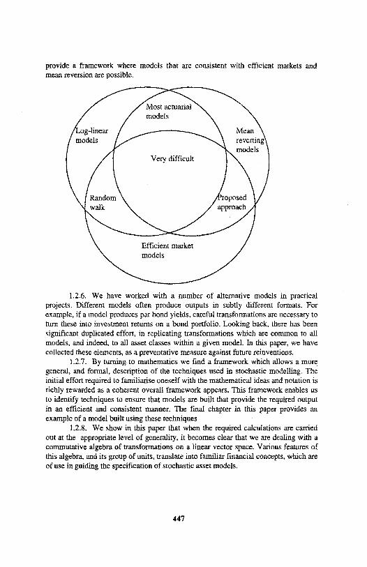
provide a framework where models that are consistent with efficient markets and mean reversion are possible.

1.2.6. We have worked with a number of alternative models in practical projects. Different models often produce outputs in subtly different formats. For example, if a model produces par bond yields, careful transformations are necessary to turn these into investment returns on a bond portfolio. Looking back, there has been significant duplicated effort, in replicating transformations which are common to all models, and indeed, to all asset classes within a given model. In this paper, we have collected these elements, as a preventative measure against future reinventions.

1.2.7. By turning to mathematics we find a framework which allows a more general, and formal, description of the techniques used in stochastic modelling. The initial effort required to familiarise oneself with the mathematical ideas and notation is richly rewarded as a coherent overall framework appears. This framework enables us to identify techniques to ensure that models are built that provide the required output in an efficient and consistent manner. The final chapter in this paper provides an example of a model built using these techniques

1.2.8. We show in this paper that when the required calculations are carried out at the appropriate level of generality, it becomes clear that we are dealing with a commutative algebra of transformations on a linear vector space. Various features of this algebra, and its group of units, translate into familiar financial concepts, which are of use in guiding the specification of stochastic asset models.

447

1.2.9. The ideas contained in this paper can be applied to continuous or discrete time models. In this paper we have only provided details of discrete time models and, for ease of exposition, we will talk in terms of years, but the logic refers just as easily to monthly or quarterly models. We have decided to concentrate on discrete time models as these allow us to present the key ideas while using a minimum of mathematical machinery. Hopefully this will enable the concepts to be appreciated by a wide audience.

2. GAUGES

2.1. Gauge definition 2.1.1. We start by developing the concept of a gauge. Broadly, a gauge

captures the features of any index which cash flows might be linked to. These could include inflation indices, foreign exchange rates, equity price or dividend indices. Such gauges form the building blocks of any stochastic investment model.

2.1.2. Formally, we define a gauge to be an object comprising two elements, which we describe below. These elements are

l a deflator {Da}

l a term structure (Pab)

2.1.3. In this notation, the subscript a denotes a valuation date. The quantities 0a and Pab are known in time for use at valuation date a, but in general, not before. The subscript b for the term structure denotes the maturity date of a bond.

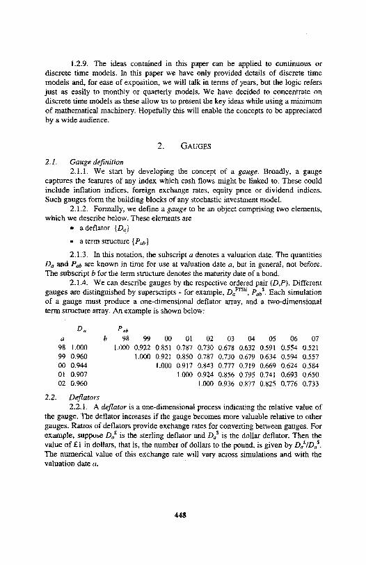
2.1.4. We can describe gauges by the respective ordered pair (D,P). Different gauges are distinguished by superscripts - for example, DaFTSE, PabS. Each simulation of a gauge must produce a one-dimensional deflator array, and a two-dimensional term structure array. An example is shown below:

Da P ab

a b 98 99 00 01 02 03 04 05 06 07 98 1.000 1.000 0.922 0.851 0.787 0.730 0.678 0.632 0.591 0.554 0.521 99 0.960 1.000 0.921 0.850 0.787 0.730 0.679 0.634 0.594 0.557 00 0.944 1.000 0.917 0.843 0.777 0.719 0.669 0.624 0.584 01 0.907 l.000 0.924 0.856 0.795 0.741 0.693 0.650 02 0.960 1.000 0.936 0.877 0.825 0.776 0.733

2.2. Deflators 2.2.1. A deflator is a one-dimensional process indicating the relative value of

the gauge. The deflator increases if the gauge becomes more valuable relative to other gauges. Ratios of deflators provide exchange rates for converting between gauges. For example, suppose is the sterling deflator and is the dollar deflator. Then the value of £1 in dollars, that is, the number of dollars to the pound, is given by The numerical value of this exchange rate will vary across simulations and with the valuation date a.

448

2.2.2. Our construction of exchange rates from deflators automatically ensures that we respect certain elementary triangular identities. For example, if I take £100 and convert it first into Euros and then into Dollars, I should (absent transaction costs) get the same answer as if I converted the £100 directly into dollars.

2.2.3. It is only the relative values of deflators which affect gauge output. This means that we have a degree of freedom to choose the absolute values of all deflators. For example, we could define to be identically equal to 1 for the Sterling gauge. Alternatively, we could choose to account in units of an index of Japanese equity prices, in which case the Japanese equity deflator would be 1 by construction, and the Sterling deflator would fluctuate in inverse proportion to the equity index and in proportion to the strength of Sterling relative to the Yen. This transformation amounts simply to a change of accounting currency or numeraire. Any such choice is arbitrary from an economic point of view (although one choice may be natural for investigating a particular problem). We will retain generality by not assigning any one deflator a special position in our description and so avoid “hard coding” a particular accounting currency.

2.2.4. It is important that exchange rates should be positive numbers. We shall therefore consider it as axiomatic that all the deflators we consider should be positive processes.

2.2.5. It is important to distinguish between the actual out-turn and various forecasts of the future. Deflators represent the realised series of exchange rates. In a simulation exercise, these should not be accessible for making decisions or for accounting purposes before the rate has been realised. Projections at a point in time cannot rely on perfect knowledge of the future, but only on the forecasts available on the commencement date of the projection. To model these forecasts, we need to consider the concept of term structures.

2.3. Term structures 2.3.1. Having considered current prices of gauges, we now consider assets

and liabilities relating to future values of gauges. Of particular interest are bonds paying regular level coupons and a principal payment at a given maturity date, all of these cash flows being expressed in units of a specified gauge. The prices of all such bonds constitute a term structure for the gauge.

2.3.2. Typically, bond prices will be expressed in units of the deflator to which the cash flows relate. These bond prices may then be re-expressed as yields. For example traditional analysis examines the ‘yield to maturity’, that is, the discount rate at which the market price of a particular bond is equal to the present value of future cash flows. This yield will typically vary by term and coupon.

2.3.3. Alternatively, the general shape of bond prices may be captured by a par yield curve, which describes the coupon rate required for a bond of given term to have a market value equal to 1. The resulting bond is sometimes called a par bond for that term. The par yield is sometimes called a swap rate.

449

2.3.4. While yield methods remain popular for some purposes, a different method of describing term structures has now become the dominant standard in the financial economics literature. This standard considers the prices of zero coupon bonds (or zeros), that is the price at time a of a bond paying one unit of the gauge at a future date b (with b ≥ a). We denote this bond price by P ab . In the next section, we relate spot rates to swap rates and various other yield definitions in common use.

2.3.5. Our convention is that bond prices are expressed in units of the underlying gauge. In some cases, for example, fixed income securities, this is entirely consistent with quotation conventions used in the market place. In other cases, we will consider gauges linked to short interest rates, or to a stream of dividends, and our convention may not seem so intuitive. This convention does, however, ensure that P aa = 1 for all a.

2.3.6. For some gauges, these bonds might be considered as a reversion, that is, an entitlement to a given gauge at some future date. This enables us to interpret bond prices not only for currencies but also for other gauges such as equities. These constructions are important in ensuring that, for example, equity prices remain in a credible relationship to dividend forecasts.

2.3.7. In the equity example, the value of a reversion on an equity price index is a required ingredient to price forward contracts derived from that index. To demonstrate the link to forward prices let us temporarily take D a

s = 1, then DaRPabR is the amount we pay now to receive D b R in the future. This can be considered in two parts,

1) the expectation of the value of the deflator at b, 2) the time value of money 2.3.8. We can see that if the required return on this risky asset is greater than

the risk free rate (RFR) then

So the forward rate is a downwards biased estimate of the future value of the deflator. If, however, no risk premium is demanded on the risky asset then the forward rate will provide an unbiased estimate of the future value of the deflator.

2.3.9. It might be thought that there is some loss of information in going from the prices of all bonds to the prices of zero coupon bond only. After all, many bond markets show a coupon effect, where bonds with different coupons have different redemption yields.

2.3.10. Fortunately, in most world markets, it is possible to find a single collection of zero prices which adequately explain bond prices of all terms and coupon rates. Otherwise, there would be arbitrage profits to be had from stripping up the cheaper bonds to reconstitute the dearer ones. However, the process of deriving zero prices from observed coupon bonds is often computationally intensive. This may explain why, prior to the advent of fast computers, the conceptual tidiness of zero

450

The forward rate

bond prices was often sacrificed in favour of the more easily computed par yields or yields to maturity.

2.3.11. While we have considered term structures in the context of bonds, the same concepts can apply to every gauge. For example, we would argue that in principle, an equity price can be expressed as the sum of the values of future dividends, even if the precise allocation of value across dividend dates may not be easily observable. In the same way, in a valuation context it may be necessary to consider the value of future inflation linked cash flows, even if no government backed inflation-linked bonds are traded.

2.4. Constraints on Term Structures 2.4.1. We can describe term structures with two dimensional arrays.

Unfortunately, to build a credible model, we must incorporate effects in at least three directions. As we have only two dimensions to play with, these three directional effects interact in subtle ways. The directions are as follows:

2.4.2. Constraints on yield curve shapes refer to the behaviour of bonds with different terms on a given valuation date. For example, it might be required that yields are positive, or that the yield curve is smooth in some sense. A parametric family of possible yield curve formulae may be specified. In any case, we would want to forbid yields from exploding to infinity for large terms (or to 100% in the case of a discount). On the other hand, it would also be normal to require that bonds decrease to zero for large terms, in such a way that the yield tends to some limiting value.

2.4.3. Arbitrage means a sure way of getting something for nothing. More specifically, an arbitrage opportunity is a selection of recommendations (both buys

451

and sells) such that, at some later date, the buys cannot have under-performed the sells. To characterise arbitrage, or its absence, we must consider fixed portfolios of bonds (that is, with fixed maturity dates) and vary the valuation date.

2.4.4. Finally, statistical analysis must be applied to comparable quantities at different points in time. For example, a statistician may consider the properties of two- year spot yields over a number of decades. In the term structure context, these yields will be derived from a series of bonds in which the difference between the valuation date and maturity date is held constant.

2.4.5. In the context of model building, it is easy to make two of these constraints work at once. For example, many models specify a family of possible yield curves, and then provide a statistical description of these curve parameters. However, unless great care is taken, arbitrage tends to creep in to such models. On the other hand, some early arbitrage-free models implied yields which were unreasonable in a statistical sense - for example by exploding to infinity for distant valuation dates. This paper provides a structured methodology for ensuring that all three constraints can be satisfied at once.

2.4.6. Actuarial work to date has concentrated on the time series properties while making a simple assumption for the yield curve. Most often a flat yield curve is assumed, in other words a geometric progression for P ab . In some cases, where few bonds are available, this may be a reasonable initial assumption. However, the assumption that future yield curves will be flat leads to a number of odd economic effects, most notably the creation of arbitrage opportunities. In general, it is more satisfactory to model the individual zeros rather than to impose a particular parametric form on the whole curve.

2.4.7. For some of the later algebra, we shall require some further regularity conditions on the yield curve shape. The conditions are:

•

• 0 exponentially fast as 2.4.8. We can see from these conditions that the processes and are

completely specified if we know their product a P The decomposition is as follows:

2.4.9. One commonly required constraint on zero coupon bond prices is that they should decrease with term. This is sometimes called the positive interest condition. We shall argue that the positive interest condition is not necessarily a universal feature of all gauges. However, gauges which do not require the positive interest condition are the exception rather than the norm, we will therefore use the term principal gauges when the positive interest constraint does not apply. We will later consider principal gauges in more detail and see precisely how these conditions can be implemented.

452

•

2.5. Yield relationships 2.5.1. One of the primary differences between competing models lies in the

choice of interest rate conventions. Arbitrage-free models typically focus on zero coupon bond prices, and the associated spot or forward yields. On the other hand, available statistics are often based around gross redemption yields or par yields, and many statistically based models follow this into the projections. The multiplicity of yield definitions are sufficiently confusing that it is worth recording some notation for later use.

2.5.2. The yields we will consider are as follows: • spot yield • forward yield • gross redemption yield r ab (g) on a bond with coupon g • par yield 2.5.3. There are many possible conventions for quoting interest rates. For our

purposes, it is most convenient to consider rates in term of a discount, that is, the interest payable annually in advance for a loan. This is related to the annualised rate i payable in arrears according to the relationship:

discount

2.5.4. The spot yield is the internal rate of return on a particular bond. Using our discount convention, we can evaluate the spot yield as:

2.5.5. The forward yield ab is the future discount rate projection which simultaneously explains all zero coupon bond prices today, so that

or, equivalently,

2.5.6. Let us consider the price at time a of a g-coupon bond maturing at time b. In the absence of arbitrage, this can be obtained by adding up the principal and interest, and discounting each cash flow at the appropriate zero coupon bond price. It turns out to be most convenient to consider bonds with interest payable in advance (as opposed to the usual convention of interest in arrears), in which case we have

coupon bond price =

2.5.7. The gross redemption yield is the single flat discount rate r at which the coupon bond price is the present value of its coupons, so that

453

2.5.8. A par bond is one for which the coupon rate is equal to the gross redemption yield. Equivalently, this implies that the bond has a market value of exactly 1. Denoting the coupon level by g, this defines the par yield by

2.5.9. There is one special case in which these yield conversions are particularly simple. For one-year yields, it is easily seen that all rates are equal, that is:

3. GAUGE TRANSFORMS

3.1. Bond examples 3.1.1. We have already considered ways of pricing coupon bonds from zero

coupon bond prices. We now take this idea further and define a new gauge. 3.1.2. To take a simple example, let us consider bonds with outstanding term

τ paying level coupons in advance at a rate g. The market price of such a bond at time a is then given by

coupon bond price =

3.1.3. Of course, this will represent a different bond for every possible valuation date a. However, this does reflect how statistics are often compiled; for example, historic yield data often focuses on the yield on a 'benchmark' bond with a term close to 10 years. As one bond gets shorter, it is replaced in the index by a new, longer bond.

3.1.4. We can think of this coupon bond as defining a new currency in its own right, which has its own deflator. Allowing for the value of the underlying currency, we can define this new deflator by

3.2. Derived term structures 3.2.1. We have developed a method for defining a new deflator, but this does

not yet fully specify a gauge, because we need to define a term structure. 3.2.2. We do not have complete freedom to specify a term structure -

whatever we specify must be consistent with the term structure of the original gauge. 3.2.3. Taking again the example of a coupon bond, we must interpret the

derived term structure P ab ' as the price, at time a, of the cashflows from the bond starting at time b. We will denote this as reversion ab . Equivalently, this is a reversion on a basket of underlying zero coupon bonds. However, it is easy to price a reversion on a zero coupon bond; the value is the same as the current price of the same bond. This is because a zero coupon bond carries no income, and so nothing is foregone by waiting longer for the bond.

454

3.2.4. Allowing for exchange rate differentials, this forces the reversion value to be of the form:

3.2.5. This gives the value of the reversion in the underlying currency; however, our term structure definition requires term structures to be expressed in units of the gauge to which they relate, which implies the following definition of

3.2.6. Substituting in for the transformed deflator, we finally have:

3.2.7. It should be noted that these gauge transforms are essentially trivial in a flat yield curve environment, because bond prices are then preserved. It is in the world of general yield curves where these transforms are most useful.

3.2.8. We can think of these transforms as acting instead on the product which contains all the information required to unpick the individual elements.

The transform then appears as follows:

3.2.9. This representation establishes that gauge transforms are essentially linear maps. Fortunately, the algebra of linear maps has received great attention from generations of mathematicians. However, we believe that our financial interpretation of this mathematics is original.

3.3. Inverse Transform 3.3.1. We have defined a gauge transform, and a number of questions

naturally arise. In particular, can we do the transform backwards? If we can show that the transform is not injective that is, different object gauges can be mapped onto a common image, then the inverse is not well defined.

3.3.2. Let us consider a simple example first, of a one year bond with a single coupon, g < 1, payable in advance. The gauge transform is then defined by

3.3.3. Let us consider changing the original term structure definition,

replacing by where k>-1 and constant. This satisfies all of our

axioms, except perhaps the positivity condition. The transformed gauge would then have a term structure given by:

455

3.3.4. This is plainly the same transformed term structure as we had before. Therefore, this gauge transform is not injective and we cannot construct an inverse transform.

3.3.5. It can also be shown that this gauge transform is not surjective either. In other words, we can find possible derived term structures P a b ' which do not correspond to any positive initial term structure The construction of such an example is left as an exercise for the reader.

3.3.6. This lack of an inverse has important consequences for modelling. The modeller usually has some freedom as to what gauges he or she subjects to statistical analysis. However, if one decides to model coupon bond prices, various awkward inequalities must be respected in order to produce a coherent model. Our desire to work with a coherent model, and also one which avoids unnecessary complexities, leads us to prefer to model zero coupon bond prices, rather than par or gross redemption yields.

3.4. Transform Algebra 3.4.1. We now consider gauge transforms in greater generality. Specifically,

for a non-negative cash flow vector we can define transformed gauges and term structures by

3.4.2. Written as a linear map, this becomes:

3.4.3. It is important to ensure that the resulting gauge is indeed a gauge, that is, that our axioms are satisfied. The only non-trivial constraint is that the infinite sums are convergent. Our original axioms for the base gauge (D,P) ensure that tends to zero exponentially fast as b tends to infinity. A necessary and sufficient condition for the above sums to converge for all such P is that

456

3.4.4. If π satisfies these conditions, then we say that π is a gauge transform. This maps the set of all possible gauges onto some other set of gauges. We have already considered the special case of transforms induced by finite term bonds. In these cases, the cash flows π, are zero from some point on, so the lim sup condition is automatically satisfied. It is important to realise that the lim sup condition does permit gauge transforms induced by cash flows that tend to infinity, the condition is satisfied as long as the rate of growth is slower than exponential. Hence a cash flow with payments π = (1,2,3,4,...) can still define a gauge transform.

3.4.5. It is useful to consider the effect of applying two gauge transforms consecutively. For example, if we apply a gauge transform v followed by another transform π. do we get the same answer as applying the opposite order? Is the result equivalent to a single gauge transform?

3.4.6. It turns out, after some algebra, that the answer to both these questions is yes - the application of transforms is commutative, and we have the identity

where π° v denotes the convolution, defined by

3.4.7. It is convenient also to consider the concept of a signed gauge transform, that is, a gauge transform where we remove the constraint that cash flows

are non-negative. To ensure convergence, we must still insist that

These signed gauge transforms are not proper gauge transforms, as for some choices of initial gauge, the resulting derived term structures may not satisfy our positivity conditions. Nevertheless, they may be able to operate on some gauges. We can continue to define convolutions of signed gauge transforms, which can be conceived as a formal algebraic construction whether or not the signed gauge transforms are useful for transforming gauges.

3.4.8. We have already seen that a coupon bond is an example of a gauge transform which we could not invert. More generally, in the context of a signed gauge transform, we can consider whether an inverse transform exists, in the form of another signed gauge transform. In particular, we will insist that any supposed inverse must still satisfy the lim sup condition. If no such inverse exists, we say that the signed gauge transform is singular. An invertible signed gauge transform is non-singular.

3.4.9. It is easily seen that the convolution of two non-singular signed gauge transforms is still non-singular. On the other hand, the convolution of any signed gauge transform with a singular signed gauge transform produces another singular signed gauge transform.

3.4.10. We can consider the transform process as purely an algebraic manipulation. However, after each inverse transform we need to test whether the conditions for a gauge are satisfied.

457

3.4.11. An example of a singular transform is that associated with a one-year bond which we previously described. It can be shown that for any finite-term bond with coupon less than 100%, the associated gauge transform is singular. However, we shall see that the perpetuity transform is non-singular.

3.5. Total returns 3.5.1. We start with a relatively simple exercise - calculating the total return

on cash. This is particularly simple because the capital return is always zero, so we need only to model the income element. We can view cash investment overnight as being a very short bond. In the context of a discrete model, we will normally wish to approximate this with the return on a series of one year bonds, each rolled over into the next. The total return between time a and time b is then given by

total return =

3.5.2. Of course, this total return is measured in units of the underlying gauge; if we want to express this in units of the numeraire for the whole model, we need to adjust for the deflator at the start and the end, giving

3.5.3. Let us now move on to total return indices for more complex bonds. We have constructed a framework for stochastic modelling of individual bond prices. However, data is often not easily available in this form. Instead, indices of bond returns are often supplied. These indices usually refer to the total returns on a bond of a particular outstanding term; as the bonds shorten over time, the old bonds are sold and then reinvested to maintain the specified outstanding term.

3.5.4. These indices are often available in three forms: a capital-only index, a total return index, and a gross redemption yield. It might be thought that the capital and total return indices could be calculated from the yield sequence, but this is not in fact the case. The reason is a subtle one - you may have a table of 10-year bond yields, but if you want the total return on a ten-year bond, you need to hold it for some period of time; one year, say. But at the end of the year, it will be a nine-year bond, so it would not be appropriate to use a ten year yield to value it. In an environment where the yield curve slopes upwards, this drift down the curve provides an important element of additional return. As a result, the average return on a rolled-over bond portfolio should typically be slightly higher than an average of gross redemption yields. Whether or not this happens for a particular model is dependent on the particular yield curve interpolation algorithm employed.

3.5.5. If we have a detailed specification of the bonds underlying an index, and the yields on those bonds, we can deduce the market value of the bonds at a point in time, and hence the running yield on the index. In principle, this enables us to split the income and capital elements of return given a total return index. In practice, these

total return =

reconciliations are often difficult to construct because of complex market conventions regarding accrued interest, which vary from country to country.

3.5.6. Let us now consider the total return on an index whose cash flow pattern is given by the gauge transform π. The price of the corresponding bond is given by the transformed gauge:

3.5.7. To construct the index, we need to be more precise about when this bond is held. We will assume that the notional bond which represents the index is rebalanced at the year end. We construct the index by considering the cash flows at the year end, before rebalancing. If we let a+1 represent the year end, then the value at the year end of the cashflows are just

3.5.8. The value of this bond at the year start - ie the same set of cashflows - will then be obtained by discounting for a further year, that is

3.5.9. The total return during the year is then the value at the end (which includes the immediate income π0) divided by the value at the start, that is,

total return during year from a to a+1 =

3.5.10. Over a period from a to b, the total return index is then given by a product:

total return from a to b=~

3.5.11. This expression clearly reduces to the total return on cash in the case where π is the identify transform.

3.6. Gauge orbits. 3.6.1. We have constructed a theory of gauges, and of gauge transforms

acting on these gauges. We have also investigated the structure of this transform algebra. We can now use this to classify gauges.

3.6.2. We say that two gauges are in the same orbit if they are related to each other by a non-singular signed gauge transform. This usage of orbit is consistent with the group-theoretic use of the term. If two gauges are in the same orbit, it is possible to compute one from the other. From a stochastic modelling point of view, we only need to generate one gauge in each orbit, the others follow automatically.

3.6.3. We can place a partial ordering on orbits as follows. If π is a singular signed gauge transform, and (D,P), are both gauges, then we say that (D,P) is in a higher orbit than It is possible to construct gauges in a lower orbit from higher orbits, but not the other way around. From the stochastic modelling point of view, it is sensible to simulate gauges in the highest orbits required, and then derive the others via gauge transforms. In particular, as gauge transforms corresponding to

459

finite term bonds are singular, it is preferable to model the structure of the zero curve, rather than coupon bonds.

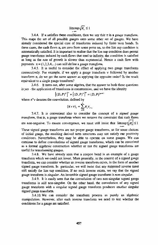
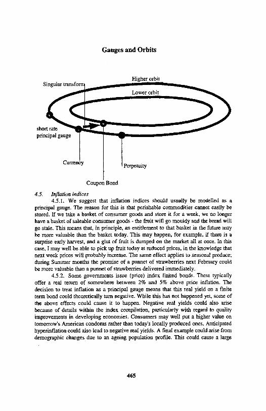
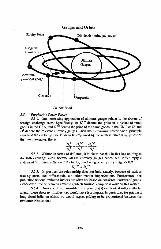
Gauges and Orbits

4. SHORT RATES AND PERPETUITIES

4.1. Short rates 4.1.1. Suppose we have a gauge in which interest rates are always positive.

We can use the short rate to define a new gauge constructed in its own right. For reasons which will later become apparent, we denote this new gauge by where

4.1.2. Equivalently, we can write the short rate of the original gauge as a ratio of two gauges:

4.1.3. We can also determine a derived term structure for this gauge; the bond prices are determined by the forward structure of interest rates. To express these forward rates in units of the new gauge, we need to discount and express in units of the derived gauge, so that

4.1.4. Of course, it does not follow that this new gauge exhibits the positive interest condition. Indeed, if short interest rates are expected to rise, we might well

460

expect to find P ab > 1 for some b, although the bond prices must eventually tend to zero with increasing term. Such gauges where positive interest is not required, are quite unusual. We refer to them as principal gauges.

4.1.5. The transformed gauge can he thought of as the result of applying a signed gauge transform, defined by the cash flow vector:

However, this signed gauge transform does not always produce a gauge, because of the negative cash flows. In fact, the necessary and sufficient condition that is a true gauge is that the original gauge (D,P) has positive interest, that is, that P ab is a strictly decreasing function of a. This should certainly be the case for currencies, for example.

4.1.6. We now revisit the expression for total returns on a bond portfolio, given by

total return =

4.1.7. Provided that the transformed gauge has positive interest, we can write the bond product as a product of discounts:

total return =

4.1.8. In discrete time, this expression appears more clumsy than the original. However, in continuous time one needs to take the limit of such infinite products, and the deflator ratio is an important intermediate step in the numerical integration of total returns.

4.2. Perpetuity transforms 4.2.1. We now consider another transform - the perpetuity transform. This is

defined by a cash flow pattern which pays one unit of cash flow every year for ever, that is:

4.2.2. The resulting transform equations are:

4.2.3. It is useful to observe that this transformed gauge does satisfy the positive interest condition, that is, bond prices P ab to decrease strictly with b. This

461

occurs because the numerator of P ab [+1] contains one term fewer each time b is

increased. 4.2.4. This transform is clearly the one required to go from a dividend index

to an equity price, or indeed from a rental income index to a property market value. We will now show why this is also relevant for modelling currencies.

4.2.5 Let us consider the application of a perpetuity transform to a short rate gauge. This gives a telescoping sum where terms cancel in pairs:

and

4.2.6. We can see that the perpetuity transform [+1] is the inverse of the deflator signed gauge transform [-1]. In particular, two gauges related by one of these transforms are in the same orbit.

4.2.7. The implications of this correspondence are profound, because they provide a characterisation of positive interest gauges, and of principal gauges. In particular, we can see that

. A gauge satisfies the positive interest condition if and only if it can be obtained as the perpetuity transform of some other gauge

. A gauge is a principal gauge if and only if it is not the perpetuity transform of some other gauge

4.2.8. The important economic counterpart of positive interest is the storage requirement. If a commodity can be stored (without cost) then it will always be more valuable to receive the commodity today than next year. If discount bond prices ever exceeded 1, then traders could create an arbitrage by buying the commodity now and selling for forward delivery. This means that gauges for storable items should have positive interest. On the other hand, principal gauges must reflect items which cannot be stored.

462

4.3. The group generated by short rates and perpetuities 4.3.1. As the short rate and perpetuity transforms are non-singular, they must

lie in the group of units of the algebra of signed gauge transforms. In particular, we can identify the subgroup generated by the perpetuity transform. This subgroup (under convolution) will be isomorphic to the integers under addition, ie there exists a l-to-1 relation. This isomorphsim is denoted by square brackets, so that an integer n is related to a signed gauge [n].

4.3.2. We have already defined the signed transforms [-1] and [+1]. The cash flow representations of the remaining transforms can be expressed in terms of binomial coefficients as follows:

4.3.3. It is easy to verify the isomorphism relationship that [m]O[n]=[m+n]. We have already seen this in the special case where m = -1 and n = +1.

4.3.4. These transforms are useful for model construction. We will see that principal gauges are easier to construct from a statistical perspective, because we do not need to ensure positivity of interest rates. Our-recommended procedure for modelling is that the short rate transform should be applied repeatedly to any positive interest gauge, until a principal gauge is obtained. This principal gauge should be modelled, and the positive interest gauges reconstructed by repeated application of the perpetuity transform. The perpetuity counter of a gauge is defined as the number of times the short rate transform is applied to achieve a principal gauge. Clearly, this is equivalent to the number of times the perpetuity transform is applied to the principal gauge to get back to the original gauge. In other words, if (D,P) = is a principal gauge, then we say that has a perpetuity counter of n.

4.4. Signed gauge transforms 4.4.1. Algebraists will appreciate that the set of signed gauge transforms are a

commutative algebra under addition and convolution. The non-singular signed gauge transforms constitute the group of units for the algebra.

4.4.2. Given a signed gauge transform π, we can &fine the generating function h?(z) where;

The condition for π to be a gauge transform, is equivalent to the

series converging for

463

4.4.3. Consider for example, the group generated by the short rate and perpetuity transforms. For all integer values of n we have . It is no

coincidence that this subgroup is isomorphic (under convolution) to the integers under addition. We can generalise to establish that ; this shows that we

have an isomorphism between the algebra of signed gauge transforms and the algebra of analytical functions on ? < 1. In particular, if π is non-singular gauge transform, then there exists an inverse v which we can calculate and satisfies

4.4.4. Now consider the gauge transform relating to a finite term bond with coupon g< 100% and term ?, hence π describes the cashflow

Then where z i are the roots of

h π (z). By equating the coefficients of the z 0 we find g = As g <1

there exists an i such that ? < 1. This root lies within the unit disc and the function

has a singularity inside the unit disc, so cannot be the generating function of a

gauge transform. This tells us that the gauge transform induced by a finite term coupon bond has no inverse and so is singular.

464

terms

Gauges and Orbits

4.5. Inflation indices 4.5.1. We suggest that inflation indices should usually be modelled as a

principal gauge. The reason for this is that perishable commodities cannot easily be stored. If we take a basket of consumer goods and store it for a week, we no longer have a basket of saleable consumer goods - the fruit will go mouldy and the bread will go stale. This means that, in principle, an entitlement to that basket in the future may be more valuable than the basket today. This may happen, for example, if there is a surprise early harvest, and a glut of fruit is dumped on the market all at once. In this case, I may well be able to pick up fruit today at reduced prices, in the knowledge that next week prices will probably increase. The same effect applies to seasonal produce; during Summer months the promise of a punnet of strawberries next February could be more valuable than a punnet of strawberries delivered immediately.

4.5.2. Some governments issue (price) index linked bonds. These typically offer a real return of somewhere between 2% and 5% above price inflation. The decision to treat inflation as a principal gauge means that this real yield on a finite term bond could theoretically turn negative. While this has not happened yet, some of the above effects could cause it to happen. Negative real yields could also arise because of details within the index compilation, particularly with regard to quality improvements in developing economies. Consumers may well put a higher value on tomorrow’s American condoms rather than today’s locally produced ones. Anticipated hyperinflation could also lead to negative real yields. A final example could arise from demographic changes due to an ageing population profile. This could cause a large

465

demand for savings switching to a large demand for consumption as the generation retires resulting in negative real yields.

4.5.3. Similar issues apply to other inflation indices, such as wages, GDP, medical expenses or insurance claims. All of these should probably be modelled as principal gauges.

4.6. Currencies 4.6.1. In the normal course of events, and in the absence of exchange

controls, currencies can be stored, and satisfy the positive interest condition. This suggests that currencies should not be treated as principal gauges.

4.6.2. Indeed, we have already established that currencies can be considered as the perpetuity transform of a short rate gauge. So we now ask the question: should the short rate gauge be a principal gauge, or should it be a perpetuity transform of something else? Equivalently, can the short rate be stored? To store a short rate, we would need to find some instrument which is worth a short rate today, and which will be worth (at least) tomorrow’s short rate tomorrow. If the market believes interest rates are likely to rise, such an arrangement will be hard to achieve. In such cases, an entitlement to tomorrow’s short rate may well be more valuable than today’s short rate.

4.6.3. This suggests that the short rate should be treated as a principal gauge. It follows that currency gauges will normally have a perpetuity counter of 1. In countries where they exist, perpetual bonds will correspond to a gauge with perpetuity counter of 2. It should perhaps be mentioned, at this point that some so-called perpetual bonds actually contain valuable early redemption options in favour of the issuer. Analysis of the options is complex; suffice to say that callable perpetuities will often be priced at a significant discount to the naïve compound interest calculation.

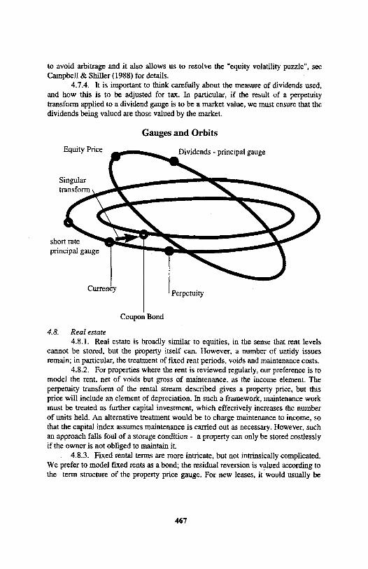
4.7. Equities 4.7.1. Equities can usually be stored. This suggests that equity price indices

should not be treated as principal gauges. Indeed, we have already argued that an equity price index is the perpetuity transform of the dividend index.

4.7.2. Is the dividend index a principal gauge? Probably it should be. After all, if I store today’s dividend, it will not miraculously turn into next year’s dividend one year later. Indeed, at times of high expected dividend growth, we may well find that au entitlement to next year’s dividend is more valuable than this year’s dividend, that is, P ab > 1. This would imply that equity price indices should have a perpetuity counter of 1.

4.7.3. The approach to valuing equities by considering the dividend income and yield is far from original. Indeed many stochastic models explicitly use dividend income and an autoregressive (AR) yield to value equities. The crucial difference is that the gauge approach recognises the term structure of the dividend yields rather than assuming a single yield. This preserves the symmetrical approach for different asset classes, and while a “dividend yield term structure” may not initially be intuitive it is quickly seen how this concept flows naturally from the gauge approach and provides a coherent structure. In particular, using a term structure approach is required

466

to avoid arbitrage and it also allows us to resolve the “equity volatility puzzle”, see Campbell & Shiller (1988) for details.

4.7.4. It is important to think carefully about the measure of dividends used, and how this is to be adjusted for tax. In particular, if the result of a perpetuity transform applied to a dividend gauge is to be a market value, we must ensure that the dividends being valued are those valued by the market.

Gauges and Orbits

4.8. Real estate 4.8.1. Real estate is broadly similar to equities, in the sense that rent levels

cannot be stored, but the property itself can. However, a number of untidy issues remain; in particular, the treatment of fixed rent periods, voids and maintenance costs.

4.8.2. For properties where the rent is reviewed regularly, our preference is to model the rent, net of voids but gross of maintenance, as the income element. The perpetuity transform of the rental stream described gives a property price, but this price will include an element of depreciation. In such a framework, maintenance work must be treated as further capital investment, which effectively increases the number of units held. An alternative treatment would be to charge maintenance to income, so that the capital index assumes maintenance is carried out as necessary. However, such an approach falls foul of a storage condition - a property can only be stored costlessly if the owner is not obliged to maintain it.

4.8.3. Fixed rental terms are more intricate, but not intrinsically complicated. We prefer to model fixed rents as a bond; the residual reversion is valued according to the term structure of the property price gauge. For new leases, it would usually be

467

assumed that the present value of rent receivable compensates the landlord for the difference between the current price gauge and the value of the reversion at the end of the term.

4.8.4. Attempts to models real estate are confounded by more than the usual level of data problems. Rental indices are often compiled from existing property portfolios, which may be on long or short leases, or more often, some unknown mixture. Published price indices are usually compiled from surveyors’ valuations, not actual transactions. This typically results in a smoother price index than would otherwise be the case. For stochastic modelling purposes, it is often appropriate to assume a more volatile price index for purchase and sales prices, with explicit smoothing being applied to simulate valuations.

4.9. Commutation functions for coupon bonds. 4.9.1. A further use of the perpetuity transform arises in the context of

coupon bonds. Let us suppose that a currency has perpetuity counter n, so that the currency gauge is represented by where (D,P) is a principal gauge.

4.9.2. Let us now consider the price of a coupon bond, of term ? and coupon g payable in advance. This corresponds to a cash flow vector of the form:

4.9.3. The transformed gauge is then of the form:

so that

and

4.9.4. We can see that all the terms involving summations can be expressed in terms of perpetuity transforms. This means that if we have generated a principal gauge in a high orbit, all required bond prices in lower orbits can be computed by perpetuity transforms. The perpetuity transforms are fulfilling the role of commutation functions in the actuarial theory of life contingencies. This results in a significant saving in the computational burden - we only need functions to return and for each principal gauge (D,P).

4.9.5. To take a practical example let us consider the total return on a rebalanced bond portfolio. The formula for this is:

468

4.9.6. In the continuous time limit, the product becomes an infinite product, whose logarithm is expressed as an integral. Even in the most analytically tractable of models, this must usually be evaluated numerically.

5. LONG BONDS

5.1. Long interest rates 5.1.1. In a previous section, we defined the following yields: • spot yield • forward yield • gross redemption yield (g) • par yield

5.1.2. We now consider the limit of these yields for large terms. We can see that if the forward rate converges to a limit for very long bonds, then the spot rate will converge to the same limit (which must be strictly positive under our axioms). We refer to this yield as the long spot yield. It is possible to construct examples, however, where this limit does not converge.

5.1.3. It is of interest to consider the effect of gauge transforms on the long spot rate. The important result is as follows. Suppose that a gauge (D,P) has a long spot rate . Then a transformed gauge ) also has a long spot rate , provided that either π is a gauge transform or π is a non-singular signed gauge transform. This means that the long spot rate can be considered not just as a property of a gauge at a point in time, but a common property to an orbit of gauges, and even to a hierarchy of ordered orbits.

5.1.4. Our axioms imply that gross redemption yields and par yields must converge for very long terms, to a common limit. This latter limit is not usually equal to the long spot yield. We refer to this as the long par yield. Taking the limit of the definition of par yield, we see that this must satisfy the relationship:

or, equivalently,

469

total return =

51.5. There is another way of viewing this yield. We can construct the short rate on the perpetuity transformed gauge as follows:

5.1.6. We can see that the short rate for the transformed gauge is simply the long par rate for the original gauge. In other words, there is nothing inherently “long” about the long par rate.

51.7. This subject has caused some confusion in the actuarial literature, which often regards long yields as solid and within actuarial scope, and short yields as fickle, subject to market sentiment, and less worth modelling. The problem arises when we consider the running yield on an equity index. We can consider this as a long par yield on the dividend gauge, in which case we are within the actuarial long term. Alternatively, the running yield is the short spot rate on the equity price gauge, in which case it is outside actuarial scope. The only real way to resolve this issue is to insist that yields of all terms are modelled at once.

5.1.8. Thus, to summarise, we have two distinct concepts of a long rate, namely:

5.2. Inverting par yield curves 5.2.1. One common method of constructing zero coupon curves involves

starting with a par yield curve, fitted to observed yields using a parametric curve family, and then working backwards. The equation for the par yield is:

5.2.2. It is more convenient to express these in terms of the perpetuity transformed gauge. Recalling the identity:

the identity becomes:

which can be rewritten as

5.2.3. It is convenient to define a quantity Gab that behaves a little like a bond price, but uses par yields where bond prices would use forward rates, that is:

470

The par yield identity then becomes:

5.2.4. Replacing b by t and summing from t = a to b-1, we can see that

5.2.5. Of course, we know that the long spot rate for the transformed gauge is equal to the long spot rate for the original gauge. The ratio on the left therefore tells us a great deal about the limiting relationship between spot and par yields. In particular, we observe:

5.2.6. Several stochastic actuarial models generate long and short par yields, which are then interpolated using exponential functions. Typically, convergence of g as

to for large s is sufficiently strong that the sum is finite. The value

produced may in principle be either greater than or less than 1, although the normal

range in practice would be within ±0.5. If the >1, then the suggested par

curve is not consistent with any positive zero prices, while if < 1 then the

long par yield is equal to the long spot yield. The ‘normal’ situation of an upwardly sloping spot curve implies which can only happen if we have an exact hit

on

5.2.7. Any model which gives the event, a probability of

zero must be regarded as problematic. Popular implementations of both the Wilkie model and the CAPLINK model allegedly suffer from this deficiency.

471

5.3. Arbitrage constraints 5.3.1. Financial theory provides some important constraints on the

movements of long spot yields. This has been considered in mathematical detail by Dybvig, Ingersoll & Ross (1994). Here, we take a more intuitive, but less formal, approach.

5.3.2. Let us suppose that I have £1 to invest at time 0. I choose to invest: • 1/2 in bonds maturing at time 1

• 1/6 in bonds maturing at time 2

• 1/12 in bonds maturing at time 3

• ...1/n(n+1) in bonds maturing at time n

5.3.3. It is easy to see that the total value of these investments adds up to the £1 I started with. At time 1, the value of the portfolio is given by:

5.3.4. Unfortunately, if the long spot rate has fallen, that is, , then this sum diverges, and we have infinite wealth. Put another way, if the long spot yield has the slightest chance of falling, then long dated bonds become very attractive investments. Of course, in a real market, this attractiveness causes their price to be bid up at time 0, pushing down the initial yield to such a point where a further fall is of negligible probability. This means that in a coherent economic model, the long spot rate should be non-decreasing.

5.3.5. In most arbitrage free models, the long spot yield is in fact constant - this must happen if the model can return (with positive probability) to its initial state. This result may seem counter-intuitive. However, published charts of yield curves, on which this intuition is based, typically show gross redemption yields or par yields. Even if the long spot rate is fixed, there is no reason why the long par yield should not vary stochastically.

5.4. Higher Order Terms 5.4.1. We have argued that the long spot rate for a given gauge (and indeed,

for a gauge orbit) should be constant over time. In such models we often find that very long dated bonds behave like a multiple of what would be expected from the long spot rate. We can therefore define a new gauge (the ultimate gauge) by the asymptotic expression:

5.4.2. This approach would appear to give some legitimacy to the actuarial practice of discounting cash flows at a ‘long term’ rate of interest, which is held constant from one valuation to the next, and then adjusting to current terms by means of a market value adjustment. However, this is only an approximation, which performs particularly badly for near dated cash flows, and which has no fundamental

472

economic justification except as a computational shortcut. With the power of modern computing, it is not clear why such shortcuts should be necessary.

5.4.3. We now seek to identify the appropriate term structure. Let us consider, therefore, the price at time a of a bond paying one unit of actuarial currency at some future time b. In units of the base gauge (D,P), this is approximately equivalent to a payment at time b of

where c is far enough away to be ‘long term’. Recall that the long spot rate is constrained by arbitrage to be a constant, so that, in particular, Thus, to value this cash flow, we need simply to value a future entitlement to a bond maturing at time c.

5.4.4. As this is a zero coupon bond, the value of this reversion is simply the value of that bond now. Thus, in units of the original gauge (D,P), the bond price at time a is:

5.4.5. Converting this into units of the ultimate gauge we see that the bond price is

5.4.6. In other words, the ultimate gauge has flat, deterministic term structure. We have shown how to project a general stochastic investment model onto a skeleton of ultimate gauges whose term structures are simple. One way of building stochastic models is to start with this ultimate gauge skeleton, and then to model market values as short term deviations from the ultimate norm.

5.4.7. The diagram below gives a schematic representation of the gauge structure. Gauges in the same orbit, ie dividends and equity prices, are related by short rate and perpetuity transforms. The transform between currency and a coupon bond is a singular transform and so the coupon bond falls into a lower orbit. Finally, in the centre we see the ultimate gauges.

473

Gauges and Orbits

5.5. Purchasing Power Parity. 5.5.1. One interesting application of ultimate gauges relates to the drivers of

foreign exchange rates. Specifically, the price of a basket of retail goods in the USA, and denote the price of the same goods in the UK. Let and

denote the relevant currency gauges. Then the purchasing power parity principle says that the exchange rate tends to be explained by the relative purchasing power of the two currencies, that is:

5.5.2. Written in terms of deflators, it is clear that this in fact has nothing to do with exchange rates, because all the currency gauges cancel out. It is simply a statement of relative inflation. Effectively. purchasing power parity suggests that

5.5.3. In practice, the relationship does not hold exactly, because of various trading costs, tax differentials and other market imperfections. Furthermore, the published national inflation indices are often not based on consistent baskets of goods, either over time or between countries, which frustrates empirical work on this matter.

5.5.4. However, it is reasonable to suppose that if one looked sufficiently far ahead, these short term influences would have less impact. In particular, for pricing a long dated inflation claim, we would expect pricing to be proportional between the two countries, so that

474

denote let

5.5.5. This implies that both inflation indices have the same long spot rate . We can also calculate the ultimate gauge for each of these, which gives:

5.5.6. This demonstrates that gauges in different orbits can still share a common ultimate gauge.

5.6. Limits of Multiple Gauge Transforms. 5.6.1. In this final section on the long term, we consider the effect of iterated

gauge transforms, that is, the repeated action of a gauge transform on a particular gauge.

5.6.2. It is helpful first to consider an approximation arising from the ultimate gauge definition. We know that for large enough b, we have by definition:

5.6.3. This suggests an approximation for gauge transforms v, provided the transform is sufficiently weighted towards distant cash flows. The approximation is

where h v denotes the generating function for the gauge transform v. 5.6.4. One special and important case arises when v is the n-fold iteration n π

of a gauge transform π. Provided that π is not the identity transform, repeated iteration of π does push most of the weight out to the long end of the yield curve, so that the ultimate gauge approximations hold. Therefore, for large n, we will have

5.6.5. The argument can be refined to show that in the limit, equality holds, so that

5.6.6. This explains why we have used the terminology ‘ultimate gauge’ - it is the ultimate limit of applying gauge transforms many times over. It is also worth noting that repeated application of gauge transforms tends to flatten the yield curve, and in the limit we have a flat yield curve model.

6. ARBITRAGE

6.1. Arbitrage 6.1.1. Financial theory defines an arbitrage opportunity as the opportunity to

make a certain future profit with zero initial investment. This could occur, for

475

example, if the same asset were priced differently in two different markets - there would then be an arbitrage to be had from buying in the cheaper market and selling in the dearer.

6.1.2. It is often a requirement of financial models that they be free of arbitrage. There are a number of reasons for this. Firstly, it is only within an arbitrage- free framework that we can construct a meaningful concept of price. If the same asset trades at different prices in different markets, which price do we model? In this paper, we implicitly invoked absence of arbitrage to justify the pricing of coupon bonds by adding up the prices of their constituent cash flows.

6.1.3. There is widespread scepticism regarding the ability of simple statistical models faithfully to replicate perceived arbitrages in the market. If a model allows arbitrage opportunities, then users of the model can make apparent sure profits by taking advantage of these opportunities. This, of course, will be misleading if these same profit opportunities do not exist in the real world.

6.1.4. Arbitrage opportunities can often sneak into models by accident rather than by design. For example, let us consider the parallel yield shift model, which underlies the concept of immunisation. This model interprets forward rates as forecasts of future short rates. New information causes changes in the expected future levels, which is uniform across all terms. This implies that that all forward rates are determined from initial forward rates by a random shift that depends only on the valuation date, so that

6.1.5. We can use this model to construct a trading strategy. Let us suppose we borrow money at time 0, on a 2-year basis, to invest in 1-year and 3 year bonds. The balance sheet might then look like this:

Maturity Maturity Present value at time 0 date value

Assets 1 3

Liabilities 2 Total PV

6.1.6. One year later, the maturity values are, of course, unchanged, but we now need to discount at time-1 bond prices, giving:

Maturity Maturity Present value at time 1 date value

Assets 1 3

Liabilities 2

476

6.1.7. Under the parallel yield shift model, we can find x 1 such that and . In this case, we can analyse the balance sheet at time 1 as

follows:

Maturity Maturity Present value at time 1 date value

Assets 1 3

Liabilities 2 Total PV

6.1.8. This result is alarming. With no initial investment, we have made a guaranteed profit - or at least, guaranteed to avoid a loss. In this situation. it is hard to see why anybody would hold 2 year bonds. It would be better always to sell those 2- year bonds and hold a mixture of 1 and 3 year bonds instead. Although the model has the advantage of simplicity, it has the disadvantage of permitting arbitrage. This arbitrage may frustrate attempts to interpret model output.

6.1.9. The real reason this arbitrage works is the simplicity of the model. If we tried to implement this with real investments, the arbitrage would fail because yield curves do not always move in parallel. In general, we usually find that there are at least as many sources of uncertainty as there are investments we might invest in. This means that we cannot in practice construct portfolios which eliminate enough uncertainty to leave a certain profit.

6.2. Forward-Backward Compatibility 6.2.1. Forward-backward compatibility is a subtle issue which arises

whenever stochastic modelling is used for decisions. It is important to ensure consistency between the basis for projecting cash flows, and the method by which those cash flows are reduced to a present value.

6.2.2. These issues arise not only in the context of stochastic models, but also in the calculation of embedded values for insurance companies. In these calculations, it might be assumed (for example) that bonds enjoy an expected return of 6% pa and equities 10% pa. All projected profits are discounted at the ‘shareholder required return' which might be 13%. This raises a number of puzzles - why would my shareholders expect my shares to return 13% when all other shares only return 10%? Is it logical that my ‘value’ as an insurer should rise if I simply sell gifts and buy equities? Given that established deterministic actuarial methods contain a number of apparent inconsistencies, it is not surprising (but still unfortunate) that the corresponding pitfalls are seldom addressed in a stochastic setting.

6.2.3. The resolution to this question can be found in the corporate finance literature. Risky assets have higher expected returns because of the additional risks they carry. These risks must be reflected in the discount rate used to value the cash flows from these risky assets. As the expected return increases so does the discount

477

rate. These rates are self-cancelling which has the logical consequence that economic value cannot be created by just switching asset classes.

6.2.4. Unfortunately the actuarial literature still appears confused on this point. This confusion is illustrated by the following quote from a recent paper by Correnti, Sonlin & Isaac (1998) presented to the Casualty Actuarial Society:-

“PCIC has traditionally invested its assets very conservatively: their current investment strategy is 20% cash and 80% bonds. ...They were interested in a 50% stock, 50% short term bond allocation. This mix seemed to offer ... additional economic value (ie an increase from $823,000 to $869,500).”

By switching from one asset-class to another it appears that economic value has miraculously been created. This is an example where the projection and discounting processes are inconsistent. In colloquial terms, this inconsistency has produced a money making machine and is a clear breach of the principle encapsulated by the phrase “$100 of equìties is worth the same as $100 of gilts”.

6.2.5. In stochastic modelling, it is important to achieve consistency between assets whose market values are projected forwards, and liabilities whose value is computed backwards by discounted cash flow. One test of such models is to see whether a theoretical matching asset portfolio does in fact match the value of liabilities on each valuation. If forward-backwards compatibility fails (as, for example, in the case of a random walk model applied to bond prices) then it will be found that the values of liabilities and matching assets diverge over time.

6.2.6. In a more general setting, stochastic models may provide many forward projections of possible outcomes. Careful analysis applied to an enterprise can reveal a joint probability distribution of many different accounting, cash flow and economic quantities at different future dates. Alternative runs under different strategies can reveal the effect of changing strategy on the probabilities of different outcomes.

6.2.7. This analysis may provide comprehensive information on distributions, but these do not tell us, on their own, which strategy is most valuable. Typically, several criteria may be examined, and a different strategy may seem best under each criterion. This process of ranking different distributions in order of preference is the backwards counterpart to the forwards projection of distributions. The backwards process of interpreting model output is rather less well developed than the construction of forward projections on which the interpretation is based. If there is a tendency to rigidity in the application of statistics to the forward projection, there is a contrasting judgmental emphasis on the backwards interpretation. It is natural to ask why we do not instead apply more judgement to the projection process and a more structured approach to model interpretation.

6.2.8. In financial theory, the forward and backward processes are more closely entwined. For example, consider the Black-Scholes model of security prices. The evolution of the probability density is governed by Kolmogorov’s forward equation (or Fokker-Planck equation). However, the arbitrage argument provides a way of pricing options, which amounts to solving the corresponding Kolmogorov backward equation (or heat diffusion equation). It is the option price which determines whether you like one strategy or another - a higher price on a set of cash

478

flows means that those cash flows are more valuable. The arbitrage argument ensures that these prices automatically reproduce the market values of traded cash flows.

6.2.9. More generally, for arbitrary Markovian models, projection corresponds to a forward equation, and interpretation to a backward equation. In Markov process theory, these equations cannot be specified independently. The mathematics is complex, and is covered in more detail in Rogers and Williams (1979). Minor technical adjustments are required to the theory in a financial context to incorporate the time value of money as well as probability. However, the conclusion is clear - it is nonsensical to characterise the forward equation as scientifically hard and the backward equation as soft. Instead, consistency dictates relationships between the two equations, either of whose formulations will contain the same mix of art and science.

6.3.10. This has important implications for model building. Conventionally ‘simple’ statistical models may result in simple forward equations. However, that may not result in a tractable backward equation. In particular, the presence or absence of arbitrage is more transparent by examination of the backward equation. If consistency is important, it makes sense to anticipate the forthcoming backward equation when constructing models for forward projection. It is important to balance ease of model construction (simple forward equation) with ease of interpretation (simple backward equation). It is a false economy to construct a simple forward model which is then excessively time-consuming to interpret.

6.2.11. In the next section we describe some of the ‘backwards’ concepts such as arbitrage and market efficiency. We will discover what constraints these imply for forward projection, and how models can be improved by balancing forward and backward aspects simultaneously.

6.3. Is your model Arbitrage free? 6.3.1. Most statistical models are in fact arbitrage free, ie there exists a

deflator. However these models are arguably arbitrage free more by accident than design. For example, many models do not provide a full term structure of interest rates, but only provide values at certain points on the yield curve, for example 1 year and 10 year interest rates. Clearly this means that the model provides insufficient information to allow annual returns on a 10-year bond to be calculated.

63.2. For practical purposes the returns on 10-year bonds may be required. so there is a need to extend the discrete points provided as outputs of the model. Unfortunately it is surprisingly difficult to extend the yield curve while preserving the arbitrage free property. Rarely do models that only provide discrete points on the yield curve come with advice on how extrapolations (or interpolation) of the yield curve should be made. As a result yield curves are usually extended in what are described as ‘practical ways’. This usually means an ad hoc mathematically simple method is used which takes no regard of economic constraints and unwanted arbitrage unintentionally enters the model. For example, models based on par yields often unintentionally generate oscillating long spot rates which generate arbitrage opportunities.

479

6.3.3. When considering any stochastic model a potential user should ask whether the model provides the full range of outputs required, and if not whether the model can be extended in a coherent manner to provide the outputs. Given the practical requirements it seems strange that if a model can easily accommodate a full term structure that it should be published in a format that only provides selected points on the yield curve.

6.3.4. It is a feature of models that they simplify reality. We capture fewer sources of uncertainty than are extant in the world out there. The arbitrage opportunities which arise are an artefact of the process of simplification. Any simple empirically based yield evolution model is likely to suffer from the same arbitrage problems, unless we actively seek to eliminate them.

6.4. Absence of Arbitrage 6.4.1. Harrison & Pliska (1981) derived the most general known

characterisation of arbitrage free models. They showed that, subject to some regularity conditions, that the absence of arbitrage is equivalent to the existence of a state price deflator, or stochastic discount function - a concept originally introduced by Arrow & Debreu (1996).

6.4.2. The stochastic discount function is a (positive) process ß a such that the market value at time a of a stochastic cash flow X due at time b is given by

market value =

where E a denotes conditional expectation given information at time a. 6.4.3. As a special case of this representation, we can see that bond prices for

each deflator must satisfy:

6.4.4. When we established the gauge framework, we mentioned that there was some arbitrariness in the choice of accounting unit, or numeraire. We could choose any deflator we wished to be an accounting currency. Equivalently, we could multiply every deflator simultaneously by a common positive process, and leave the model essentially unchanged.

6.4.5. We now avail ourselves of this opportunity, to choose a scaling factor which will make models easy to build. We decide to multiply all deflators by the Arrow-Debreu stochastic discount function, so that for each deflator D a is replaced by ß a D a . The revised equation for valuing bonds now becomes:

6.4.6. More generally, if we have a cash flow X payable at time b in units of a gauge (D,P), the market value at time a is given by

market value =

480

6.4.7. This shows how each deflator D acts as an Arrow-Debreu state price deflator for cash flows denominated in its own gauge. This should also clarify why, at the very start, we referred to the Da processes as “deflators”.

6.4.8. This observation allows a great economy in model building. A stochastic investment model is completely specified if we can specify the deflators for each gauge - the term structures then follow by conditional expectation. Indeed, we do not even need to specify all deflators, but only one for each gauge orbit.

6.4.9. As an aside, we can write perpetuity transformed term structures explicitly in terms of the original deflators; this is

Readers may recognise this as a discrete version of Flesaker & Hughston's 1996martingale representation of positive interest models.

6.5. Fisher Effects 6.5.1. The ‘Fisher relation’ for interest rates expresses nominal yields as

anticipated inflation plus a required real return. Equivalently, the difference between observed bond yields and the real return on index linked bonds, provides a forecast of inflation. We can write this in terms of gauges as

6.5.2. The right hand side is simply the forward value of inflation; the Fisher relation says in effect that forward prices are estimates for future spot prices. At first sight this may seem messy to implement, as it seems to imply causal relationships between gauges - in particular, it suggests that we should not consider a sterling gauge until we have already built an inflation model.

6.5.3. The Gordon growth model provides a similar result in the case of equities, expressing the dividend yield as the difference between expected dividend growth and a suitable discount rate. Corresponding hypotheses can be framed for any pair of gauges.

6.5.4. Using the arbitrage-free framework above, we can express bond prices in terms of conditional expectations, and the Fisher effect can be written as

forecast a

6.5.5. Written in this way, it seems hard to imagine how this condition could fail. But in fact, for many models it often does. We do not necessarily get a good estimate of a fraction from estimates of the numerator and the denominator separately. In fact, we have the relationship:

481

6.5.6. We can see that the Fisher effect approximately holds provided that the covariance term is small. Otherwise, the Fisher effect may not hold.

6.5.7. The Fisher relation is a good example of how imposing a model initially can override possible economic constraints.

6.5.8. For example, let us suppose that we had developed a model where log par yields and log prices were jointly linear. Then, in particular, expected log inflation would depend linearly both on the log nominal yield and also the log real yield.

6.5.9. However, the Fisher effect would imply that expected log inflation should be linear in the yields themselves, rather than in the log yield. As a consequence, expected inflation should be convex in log nominal yields and concave in log nominal yields. Now it may be that statistical analysis of historic data cannot detect this non-linearity, but optimising portfolio selections most certainly will. If the log linear model gets the correct slope in these relationships but ignores the convexity, it will tend to overstate expected inflation when nominal yields are close to their ‘normal level’, and when real yields are either higher or lower than normal.

6.5.10. These effects are second-order, and therefore can be quite subtle to spot. In particular, the existence of mean reversion in yields does not contradict market efficiency. Instead, it is the convexity of mean reversion relationships which is important. Our gauge transformations appear to cope better in this regard than conventional log-linear techniques.

6.5.11. It is interesting that in his stochastic model, Wilkie (1995) imposes Fisher effects for expected inflation on an otherwise log-linear model. However, this imposition of market efficiency is not applied consistently - for example, the corresponding equity market relationships are not imposed. Furthermore, the transformations Wilkie applies in order to allow Fisher relations, have other undesirable consequences, such as forbidding negative real yields (which should be permitted) and permitting negative nominal yields (which should be forbidden).

6.6. Risk and Return. 6.6.1. The semi-strong version of the Efficient Market Hypothesis (EMH)

states that all publicly available price relevant information is immediately incorporated into market prices. In other words, an efficient market is one in which returns correspond in some logical way to risks borne. In such a market, an optimising investor will take a passive approach to investment management.

6.6.2. The opposite of an efficient market is an inefficient one, where the risk premia attached to different classes fluctuate significantly from one year to the next. In an inefficient market, optimising investors will continually reallocate their assets to take advantage of the most generous risk premia.

6.6.3. It is helpful to consider the expected returns on an investment denominated in units of a gauge Da. Let us suppose the return factor on holding that

482

investment between a and b is given by measured in units of the gauge. Then it follows immediately from the definition of covariance that:

6.6.4. We can see that a risk premium is obtained for taking risks that are negatively correlated with changes in the deflator. If we want to show a positive equity risk premium, we would expect that the currency deflator should go up when the equity market falls and vice versa.

6.6.5 An efficient market will result if the risk premia on different asset classes are stable through time. In other words, if the variance-covariance structure of different deflators does not change greatly over short periods, then we have the makings of an efficient market model.

6.6.6. This corresponds neatly to statistical notions of simplicity. A statistically simple model is one where the variance-covariance structure does not change. For example, most linear autoregressive or moving average models fall into this category. If we try to fit these statistical models to deflators, then we are likely to end up with an efficient market models. This means that economics and statistics are in harmony - a simple model in one framework is also a simple model in the other. It avoids the dilemma of log-linear models, where one has to choose between a theoretically watertight model with little empirical power, or an empirically based model whose consequences are theoretically inexplicable.

6.6.7. Of course, it may turn out that the construction of a statistically adequate model requires a strongly time-varying covariance structure. In that case, we would have evidence of time varying risk premia, and hence, potentially, of tactical trading opportunities.

7. BUILDING A SIMPLE MODEL

7.1. Guidelines for Building Models 7.1.1. Having laid much groundwork, we will now illustrate the approach by

building a simple asset model. To keep the complexity to a minimum, we will base it entirely on random walks and first order autoregressive (AR1) processes.

7.1.2. Observations to be borne in mind include: · gauges in higher orbits should be generated first ·principal gauges should be generated before non-principal gauges ·it is only necessary to specify deflator models; term structures follow directly 7.1.3. This suggests that we should concentrate on the specification of

deflators for principal gauges. The requirements for such processes are simple - they should be positive, and tend exponentially to zero in mean. There is no requirement for positive interest.

7.1.4. Having identified the conditions for deflators which will ensure that the economic constraints are complied we are left with a degree of freedom which we can

483

use to choose a tractable form for our deflators. To make the structure analytically simple we will require that log deflators are linear statistical models.

7.1.5. Note that this is very different from the traditional log-linear models which we identified in sections 1.1.3 and 1.1.4. In the traditional approach the log- linear framework was superimposed at the start without regard for economic constraints. By contrast in the gauge approach the economic constraints are respected and the degrees of freedom remaining after the structure has been developed can then be used to maximise analytical tractability. The requirement that deflators are log- linear does not compromise the economic constraints.

7.2. A Possible Principal Gauge Specification 7.2.1. We now consider a possible structure for a principal gauge. In order to

do this, we must specify error distributions and how these are combined to give deflators and gauges.

7.2.2. The basic unit of our approach is a driver, that is, a sequence of independent, identically distributed random variables. The jth driver is then denoted by the sequence = 1,2,3,.. .}. Without loss of generality, we may assume that these variables have zero mean and unit variance.

7.2.3. It will become necessary to use the moment generating functions of these drivers, denoted by

7.2.4. We also need to define random walks and autoregressive processes These are defined by initial conditions = 0, and the recurrence relations:

where Aj is a mean reversion parameter with 0 < Aj < 1. It is then easily shown that for a<b, we have

7.2.5. These are the simplest possible stochastic processes from which to build an asset model. Assume that deflators Da are obtained by an exponential transform from these original processes. Specifically, for constants and

7.2.6. We now seek to derive the corresponding term structures. For can write the deflator as:

484

we

assume thatwe

Which enables us to determine the conditional expectation:

7.2.7. This enables us to deduce bond prices:

But the bond prices at time 0 are part of the initial inputs. Setting a = 0, we can use these to calibrate the unknown constant c, giving:

7.2.8. Substituting back, we can see that deflators and term structures are given by:

and

7.2.9. Finally, if a ≤ b-a-1 we can cancel some terms in the upper and lower products, to give the final bond price formula:

7.2.10. This formula illustrates several noteworthy points. Let us observe firstly that the formula for contains references only to and not to .This is

485

reassuring, as a bond price at time a must depend only on information knowable on the pricing date a. Furthermore, we see that the random walk processes Wja only appear in the deflators and not in the bond prices. Again, this is sensible; if bond prices are to be mean reverting, they must not involve references to a non-stationary random walk process. It is easily seen that these terms satisfy the conditions for a gauge, provided that the initial term structure is positive and tends to zero exponentially fast for large a. In particular, we can see this formula reproduces thespecified initial term structure, and also that 1 as it should. Observant readersmay spot that our bond formula is essentially a discrete time version of the Hull-White formula [Hull & White 1990]. But, remarkable as it is, this bond price formula does not guarantee positive interest. In other words, it is a suitable model for a principal gauge, but to derive positive interest gauges we need to apply a perpetuity transform.

7.2.11. In this section, we have constructed only the principal gauges. Other gauges are derived using gauge transforms. However, in many cases, this requires infinite summations, for which a suitable numerical approach may be appropriate to accelerate the convergence. 7.2.11 We conclude this section by examining the implied ultimate gauges. These aredefined as follows:

This enables us to deduce that

7.2.12 We can see that all the mean reverting terms cancel, and we are left with a pure geometric random walk for the ultimate gauge.

8. CONCLUDING REMARKS

8.1.1. In this paper we have highlighted the considerations that need to be taken into account if a coherent stochastic investment model is to be produced. We

486

=

have built a mathematical framework that simultaneously takes account of the different economic, statistical and practical constraints. These differing constraints make it imperative that a holistic approach is taken to modelling rather than concentrating on one particular feature, which leaves the other aspects of the model to chance. This necessitates paying closer attention to the theory behind a model before getting your hands dirty with the actual building process.

8.1.2. The approach presented is generic and provides a mechanism for classifying all stochastic models. Its successful application provides a framework for comparing models in the future and provides a methodology for generating the required outputs without having to waste time and effort in repeating transformations that are common to all models.

8.1.3. We would like to thank Andrew Inchley, Jeroen van Bezooyen, Shyam Mehta, Scott Collings and Elliot Varnell for their helpful discussions on earlier drafts of this paper. We should also thank model users in various countries for constructive feedback on our faltering attempts to explain models we build. Finally, thanks are owed to Richard Chapman for his continual support, without whom this paper would not have seen the light of day. Any remaining errors are the sole responsibility of the authors.

BIBLIOGRAPHY

Arrrow, K and G Debreu (1954). Existence of an Equilibrium for a Competitive Economy Economietrica 22:265-290

Dybvig, Ingersoll & Ross (1996). Long Forward and Zero-Coupon Rates Can Never Fall. Journal of Business, vol 69, # l pp 1-25.

Campbell, J.Y. and Shiller, R.J. (1988). Stock Pirces, Earnings and Expected Dividends. Journal of Finance 43 pp 661-676.

Correnti, Sonlin & Isaac (1998) "Applying a DFA model to Improve Strategic Business Decisions". CAS DFA seminar, Boston.

Flesaker,B. Hughston, L. (1996) “Positive Interest” Risk 9(1) 46-49 Harrison & Pliska (1981) “Martingales and Stochastic Integrals in the Theory of

Continuous trading” Stochastic Processes and their Applications 11 Hull and White (1990) “Pricing Interest rate derivative securities” Review of

Financial Studies 3,4 Hull (1997) “Options futures and other Derivatives”, Prentice Hall Heath Jarrow and Morton (1990) “Bond Pricing and the term structure of interest

rates” Journal of Financial and Quantitative Analysis 25 Rogers and Williams (1979) “Diffusions, Markov Processes, and Martingales Volume

One: Foundations” Wilkie (1995) “More on a Stochastic Asset Model for Actuarial Use” British

Actuarial Journal Vol 1, Part 5

487