39

A Survey on Social Media Anomaly Detection

ROSE YU, University of Southern CaliforniaHUIDA QIU, University of Southern CaliforniaZHEN WEN, GoogleCHING-YUNG LIN, IBM ResearchYAN LIU, University of Southern California

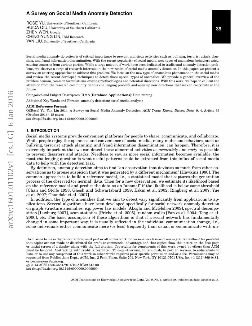
Social media anomaly detection is of critical importance to prevent malicious activities such as bullying, terrorist attack plan-ning, and fraud information dissemination. With the recent popularity of social media, new types of anomalous behaviors arise,causing concerns from various parties. While a large amount of work have been dedicated to traditional anomaly detection prob-lems, we observe a surge of research interests in the new realm of social media anomaly detection. In this paper, we present asurvey on existing approaches to address this problem. We focus on the new type of anomalous phenomena in the social mediaand review the recent developed techniques to detect those special types of anomalies. We provide a general overview of theproblem domain, common formulations, existing methodologies and potential directions. With this work, we hope to call out theattention from the research community on this challenging problem and open up new directions that we can contribute in thefuture.

Categories and Subject Descriptors: H.2.8 [Database Applications]: Data mining

Additional Key Words and Phrases: anomaly detection; social media analysis

ACM Reference Format:Qi(Rose) Yu, Yan Liu 2014. A Survey on Social Media Anomaly Detection. ACM Trans. Knowl. Discov. Data. 9, 4, Article 39(October 2014), 18 pages.DOI:http://dx.doi.org/10.1145/0000000.0000000

1. INTRODUCTIONSocial media systems provide convenient platforms for people to share, communicate, and collaborate.While people enjoy the openness and convenience of social media, many malicious behaviors, such asbullying, terrorist attack planning, and fraud information dissemination, can happen. Therefore, it isextremely important that we can detect these abnormal activities as accurately and early as possibleto prevent disasters and attacks. Needless to say, as more social information becomes available, themost challenging question is what useful patterns could be extracted from this influx of social mediadata to help with the detection task.

By definition, anomaly detection aims to find “an observation that deviates so much from other ob-servations as to arouse suspicion that it was generated by a different mechanism” [Hawkins 1980]. Thecommon approach is to build a reference model, i.e., a statistical model that captures the generationprocess of the observed (or normal) data. Then for a new observation, we estimate its likelihood basedon the reference model and predict the data as an “anomal” if the likelihood is below some threshold[Chan and Stolfo 1998; Ghosh and Schwartzbard 1999; Eskin et al. 2002; Ringberg et al. 2007; Yueet al. 2007; Chandola et al. 2007].

In addition, the type of anomalies that we aim to detect vary significantly from applications to ap-plications. Several algorithms have been developed specifically for social network anomaly detectionon graph structure anomalies, e.g. power law models [Akoglu and McGlohon 2009], spectral decompo-sition [Luxburg 2007], scan statistics [Priebe et al. 2005], random walks [Pan et al. 2004; Tong et al.2006], etc. The basic assumption of these algorithms is that if a social network has fundamentallychanged in some important way, it is usually reflected in the individual communication change, i.e.,some individuals either communicate more (or less) frequently than usual, or communicate with un-

Permission to make digital or hard copies of part or all of this work for personal or classroom use is granted without fee providedthat copies are not made or distributed for profit or commercial advantage and that copies show this notice on the first pageor initial screen of a display along with the full citation. Copyrights for components of this work owned by others than ACMmust be honored. Abstracting with credit is permitted. To copy otherwise, to republish, to post on servers, to redistribute tolists, or to use any component of this work in other works requires prior specific permission and/or a fee. Permissions may berequested from Publications Dept., ACM, Inc., 2 Penn Plaza, Suite 701, New York, NY 10121-0701 USA, fax +1 (212) 869-0481,or permissions@acm.org.c© 2014 ACM 1556-4681/2014/10-ART39 $15.00DOI:http://dx.doi.org/10.1145/0000000.0000000

ACM Transactions on Knowledge Discovery from Data, Vol. 9, No. 4, Article 39, Publication date: October 2014.

arX

iv:1

601.

0110

2v1

[cs

.LG

] 6

Jan

201

6

usual individuals. However, this could be an over-simplification of the social media anomalies withoutconsidering several important aspects of social media data.

One of the challenges that differentiate social media analysis from existing tasks in general textand graph mining is the social layer associated with the data. In other words, the texts are attached toindividual users, recording his/her opinions or activities. The networks also have social semantics, withits formation governed by the fundamental laws of social behaviors. The other special aspect of socialmedia data is the temporal perspective. That is, the texts are usually time-sensitive and the networksevolve over time. Both challenges raise open research problems in machine learning and data mining.Most existing work on social media anomaly detection have been focused on the social perspective. Forexample, many algorithms have been developed to reveal hubs/authorities, centrality, and communitiesfrom graphs [Kleinberg 1999; Erosheva et al. 2004; Song et al. 2005; Lappas et al. 2009]; a good body oftext mining techniques are examined to reveal insights from user-generated contents [Blei et al. 2003;Rosen-Zvi et al. 2004]. However, very few models are available to capture the temporal aspects of theproblem [Blei and Lafferty 2006; Hanneke and Xing 2007; Kolar et al. 2010], and among them evenfewer are practical for large-scale applications due to the more complex nature of time series data.

Existing work on traditional anomaly detection [Chandola et al. 2012; Cheng et al. 2009; Chandolaet al. 2007; Tong et al. 2008a; Guralnik and Srivastava 1999; Takeuchi and Yamanishi 2006; Ducheneet al. 2004; Lin et al. 2003; Keogh et al. 2005; Yankov et al. 2008; Cheng et al. 2009; Wong et al.2003] have identified two types of anomalies: one is “univariate anomaly” which refers to the anomalythat occurs only within individual variable, the other is “dependency anomaly” that occurs due to thechanges of temporal dependencies between time series. Mapping to social media analysis scenario, wecan recognize two major types of anomalies:

— Point Anomaly: the abnormal behaviors of individual users— Group Anomaly: the unusual patterns of groups of people

Examples of point anomaly can be anomalous computer users [Schonlau et al. 2001], unusual onlinemeetings [Horn and Willett 2011] or suspicious traffic events [Ihler et al. 2006]. Most of the existingwork have been devoted to detecting point anomaly. However, in social network, anomalies may notonly appear as individual users, but also as a group. For instance, a set of users collude to create falseproduct reviews or threat campaign in social media platforms; in large organizations malfunctioningteams or even insider groups closely coordinate with each other to achieve a malicious goal. Groupanomaly is usually more subtle than individual anomaly. At the individual level, the activities mightappear to be normal [Chandola et al. 2007]. Therefore, existing anomaly detection algorithms usuallyfail when the anomaly is related to a group rather than individuals.

We categorize a broad range of work on social media anomaly detection with respect three criteria:

(1) Anomaly Type: whether the paper detects point anomaly or group anomaly(2) Input Format: whether the paper deals with activity data or graph data(3) Temporal Factor: whether the paper handles the dynamics of the social network

In the remaining of this paper, we organize the existing literature according to these three criteria.The overall structure of our survey paper is listed in table I. We acknowledge that the papers weanalyze in this survey are only a few examples in the rich literature of social media anomaly detection.References within the paragraphs and the cited papers provide broader lists of the related work.

We can also formulate the categorization in Table I using the following mathematical abstraction.Denote the time-dependent social network as G = V (t),Wv(t), E(t),We(t), where V is the graph ver-tex,Wv is the weight on the vertex,E is the graph edge andWe is the weight on the edge. Point anomalydetection learns an outlier function mapping from the graph to certain sufficient statistics F : G→ R.A node is anomalous if it lies in the tail of the sufficient statistics distribution. Group anomaly detec-tion learns an outlier function mapping from the power set of the graph to certain sufficient statisticsF : 2|G| → R. Activity based anomaly detection collapses the edge set E(t) and weights We(t) to beempty. Static graph-based approaches fix the time stamp of the graphs as one. Now each of the methodsummarized in the table is essentially learning a different F or using some projection (simplification)of the graph G. The projection trades-off between model complexity and learning efficiency.

2

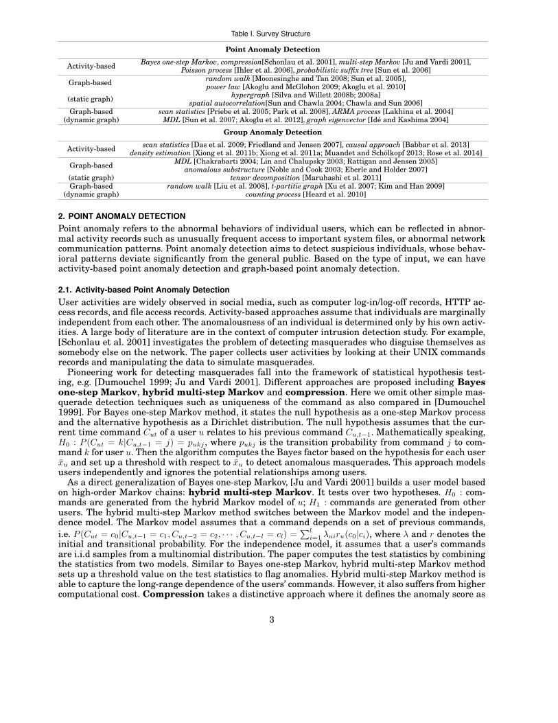
Table I. Survey Structure

Point Anomaly Detection

Activity-based Bayes one-step Markov, compression[Schonlau et al. 2001], multi-step Markov [Ju and Vardi 2001],Poisson process [Ihler et al. 2006], probabilistic suffix tree [Sun et al. 2006]

Graph-based random walk [Moonesinghe and Tan 2008; Sun et al. 2005],power law [Akoglu and McGlohon 2009; Akoglu et al. 2010]

(static graph) hypergraph [Silva and Willett 2008b; 2008a]spatial autocorrelation[Sun and Chawla 2004; Chawla and Sun 2006]

Graph-based scan statistics [Priebe et al. 2005; Park et al. 2008], ARMA process [Lakhina et al. 2004](dynamic graph) MDL [Sun et al. 2007; Akoglu et al. 2012], graph eigenvector [Ide and Kashima 2004]

Group Anomaly Detection

Activity-based scan statistics [Das et al. 2009; Friedland and Jensen 2007], causal approach [Babbar et al. 2013]density estimation [Xiong et al. 2011b; Xiong et al. 2011a; Muandet and Scholkopf 2013; Rose et al. 2014]

Graph-based MDL [Chakrabarti 2004; Lin and Chalupsky 2003; Rattigan and Jensen 2005]anomalous substructure [Noble and Cook 2003; Eberle and Holder 2007]

(static graph) tensor decomposition [Maruhashi et al. 2011]Graph-based random walk [Liu et al. 2008], t-partitie graph [Xu et al. 2007; Kim and Han 2009]

(dynamic graph) counting process [Heard et al. 2010]

2. POINT ANOMALY DETECTIONPoint anomaly refers to the abnormal behaviors of individual users, which can be reflected in abnor-mal activity records such as unusually frequent access to important system files, or abnormal networkcommunication patterns. Point anomaly detection aims to detect suspicious individuals, whose behav-ioral patterns deviate significantly from the general public. Based on the type of input, we can haveactivity-based point anomaly detection and graph-based point anomaly detection.

2.1. Activity-based Point Anomaly DetectionUser activities are widely observed in social media, such as computer log-in/log-off records, HTTP ac-cess records, and file access records. Activity-based approaches assume that individuals are marginallyindependent from each other. The anomalousness of an individual is determined only by his own activ-ities. A large body of literature are in the context of computer intrusion detection study. For example,[Schonlau et al. 2001] investigates the problem of detecting masquerades who disguise themselves assomebody else on the network. The paper collects user activities by looking at their UNIX commandsrecords and manipulating the data to simulate masquerades.

Pioneering work for detecting masquerades fall into the framework of statistical hypothesis test-ing, e.g. [Dumouchel 1999; Ju and Vardi 2001]. Different approaches are proposed including Bayesone-step Markov, hybrid multi-step Markov and compression. Here we omit other simple mas-querade detection techniques such as uniqueness of the command as also compared in [Dumouchel1999]. For Bayes one-step Markov method, it states the null hypothesis as a one-step Markov processand the alternative hypothesis as a Dirichlet distribution. The null hypothesis assumes that the cur-rent time command Cut of a user u relates to his previous command Cu,t−1. Mathematically speaking,H0 : P (Cut = k|Cu,t−1 = j) = pukj , where pukj is the transition probability from command j to com-mand k for user u. Then the algorithm computes the Bayes factor based on the hypothesis for each userxu and set up a threshold with respect to xu to detect anomalous masquerades. This approach modelsusers independently and ignores the potential relationships among users.

As a direct generalization of Bayes one-step Markov, [Ju and Vardi 2001] builds a user model basedon high-order Markov chains: hybrid multi-step Markov. It tests over two hypotheses. H0 : com-mands are generated from the hybrid Markov model of u; H1 : commands are generated from otherusers. The hybrid multi-step Markov method switches between the Markov model and the indepen-dence model. The Markov model assumes that a command depends on a set of previous commands,i.e. P (Cut = c0|Cu,t−1 = c1, Cu,t−2 = c2, · · · , Cu,t−l = cl) =

∑li=1 λuiru(c0|ci), where λ and r denotes the

initial and transitional probability. For the independence model, it assumes that a user’s commandsare i.i.d samples from a multinomial distribution. The paper computes the test statistics by combiningthe statistics from two models. Similar to Bayes one-step Markov, hybrid multi-step Markov methodsets up a threshold value on the test statistics to flag anomalies. Hybrid multi-step Markov method isable to capture the long-range dependence of the users’ commands. However, it also suffers from highercomputational cost. Compression takes a distinctive approach where it defines the anomaly score as

3

the additional compression cost to append the test data to the training data. Formally, the score isx = compress(C, c) − compress(C), where C is the training data, c is the testing data. The methodapplies the Lempel-Ziv algorithm for the compression operation. However, it can hardly capture thedependencies in the data instances.

[Sun et al. 2006] proposes probabilistic suffix tree (PST) to mine the outliers in a set of sequencesS from an alphabet Σ. It makes Markov assumption on the sequences and encodes the variable lengthMarkov chains with syntax similar to Probabilistic Suffix Automata. In PST, an edge is a symbol in thealphabet and a node is labeled by a string. The probabilistic distribution of each node represents theconditional probability of seeing a symbol right after the string label. An example of such PST is shownin Figure 1. The algorithm first constructs a PST and then computes a similarity measure score SIMN

based on marginal probability of each sequence over the PST. Then it selects the top k sequenceswith lowest SIMN scores as outliers. Since PST encodes a Markov chain, which has been shown tohave certain equivalence to the Hidden Markov model, the outliers detected by PST are similar tothose using Markov model testing statistics. Though PST construction and SIMN are relative cheap incomputation, one drawback is that PST is pre-computed for a fixed alphabet. Pre-computation makesPST less adaptive to the unseen symbols outside of the alphabet or newly coming sequences, whichbasically requires recomputing the entire tree.

Fig. 1. A example of PST. For each node, top array shows the probability distribution. Inside the node shows the label string,the number of times it appears in the data set and the empirical probability. [Sun et al. 2006]

0.008

(0.991, 0.009)

0.570

(0.968, 0.032)

0.066

(0.972, 0.028)

0.612

(0.5, 0.5)

0.005(0.755, 0.245)

(0.2, 0.8)

0.003

0.320

(0.159, 0.841)

0.388

(0.606, 0.394)

0.017

(0.155, 0.845)bb 1781

0.348

(0.612, 0.388)

Root

(0.5, 0.5)

0.023

(0.667, 0.333)

0.023

minCount = 25 (0.999, 0.001)a 4674

b 2961

aa 2920

ba 336

ab 85

aba 20

bab 7

abb 13

bbb 836

babb 4

bbab 4

a

a

a

b

b

b

b

b

a

b

b

b

a

b

0.059bba 153

(0.947, 0.053)

(1.0, 0)aaa 1356

0.520(0.333, 0.667)

baa 2120.081

a

Pmin = 0.02

Figure 1: An example of PST and pruning it usingMinCount or Pmin. The probability distributionvectors are shown on the top of the nodes, and the labelstrings, the number of times they appear in the datasetand their empirical probability are shown within thenodes

The node also records a probability distribution vectorof the symbols, which corresponds to the conditionalprobabilities of seeing a symbol right after the labelstring in the dataset. For example, the probabilityvector for the node labelled bba is (0.947,0.053). Thismeans the conditional probability of seeing a right afterbba (P (a|bba)) is 0.947, and seeing b right after bba(P (b|bba)) is 0.053.

The structure of PST is similar to the classicalsuffix tree (ST). However, there are some importantdifferences. Besides keeping a probability distributionvector at each node, in a PST, the parent of a node is asuffix of the node, while in a classical ST the parent ofa node is a prefix of the node.

2.1 Pruning of a PSTThe size of a PST is a function of the cardinality ofthe alphabet (|Σ|) and maximum memory length L. Afully grown unchecked PST is (O(|Σ|L). Several pruningmechanisms have to be employed to control the size ofthe PST.

Bejerano and Yona [5] have proposed a two-stepmechanism to prune a PST. In the first step, anempirical probability threshold Pmin is used to decidewhether to extend a child node. For example, at the

node labelled bb, if P (abb) ≥ Pmin, the node withlabel string abb will be added to the PST under someconditions. Otherwise, the node itself, including all itsdescendants will be ignored. The formula of computingP (abb) is listed in Table 1

In the second step, a tree depth threshold L isemployed to cut the PST. This means when the lengthof the label string of a node reaches L, its children nodeswill be pruned.

Instead of using Pmin, Yang and Wang [15] sug-gested the use of minCount for pruning a PST. Foreach node, the number of times its label string appearsin the database is counted. If this number is smallerthan minCount, then the node (and therefore all itschildren) are pruned.

In Figure 1 both Pmin and MinCount are shownin each node for ease of exposition. However, it is notnecessary to keep them in the PST. The dashed andthe solid lines show examples of pruning the PST usingPmin = 0.02 and MinCount = 25 respectively.

2.2 Computing Probabilities Using a PSTThe probability associated with a sequence s over a PSTis PT (s) = PT (s1)P

T (s2|s1) . . . PT (sl|s1s2...sl−1). ThePST allows an efficient computation of these intermedi-ate conditional probability terms.

For example let us compute PT (b|abab) from thePST in Figure 1. The search starts from the rootand traverse along the path → b → a → b, whichis in the reverse order of string abab. The searchstops at the node with label bab, because this is thelongest suffix of abab that can be found in the PST,and PT (b|abab) is estimated by PT (b|bab) = 0.8. Thus,we are exploiting the short memory feature, whichoccurs in sequences generated from natural sources: theempirical probability distribution of the next symbol,given the preceding subsequence, can be approximatedby observing no more than the last L symbols in thatsubsequence [12, 5].

If the PST is pruned using minCount = 25, thesearch stops at the node with label ab and PT (b|abab)is estimated by PT (b|ab) = 0.394. The following is anexample to compute the probability of string ababb overthe PST pruned using minCount = 25.

PT (S) = PT (a)PT (b|a)PT (a|ab)PT (b|aba)PT (b|abab)= 0.612× 0.028× 0.606× 0.032× 0.394= 1.309 ∗ 10−4

Since the probabilities are multiplied, care must betaken to avoid the presence of zero probability. Thus,a smoothing procedure is employed across each nodeof the PST and the probability distribution vector is

97

[Ihler et al. 2006] investigates Markov-modulated Poisson process to address the specific problemof event detection on time-series of count data. The algorithm assumes the count at time t, denotedas N(t), is a sum of two additive processes: N(t) = N0(t) + NE(t), where N0(t) denotes the number ofoccurrences attributed to the “normal” behavior and NE(t) is the “anomalous” count due to an eventat time t. More concretely, the periodic portion of the time series counts can be taken as “normal”behavior while the rare increase in the number of counts can correspond to the “anomalous” behavior.For both processes, the paper develops a hierarchical Bayesian model. In particular, the paper modelsperiodic counting data (i.e. normal behavior) with a Poisson process and models rare occurrences (i.e.anomaly behavior) via a binary process. The algorithm then uses the MCMC sampling algorithm toinfer the posterior marginal distribution over events. It uses the posterior probability as an indicatorto automatically detect the presence of unusual events in the observation sequence. The paper appliesthe model to detect the events from free-way traffic counts and the building access count data. Themethod takes a full Bayesian approach as a principled way to pose hypothesis testing. However, it

4

treats each time series as independent and fails to consider the scenario where multiple time seriesare inter-correlated.

Another application in social network anomaly detection is proposed in [Horn and Willett 2011].The paper proposes to detect unusual meetings by investigating the presence of meeting participants.Specifically, for each time stamp t = 1, 2, · · · , the inputs are given as a snapshot of the network in theform of a binary string xt = (xt(1), · · · , xt(n)) ∈ 0, 1n, where xt(j) = 0 or 1 indicates whether thejth person participated in the meeting at time t as well as the feedback from expert system with thecorrect labels yt ∈ −1,+1. The algorithm outputs a binary label for each network state yt ∈ −1,+1according to whether or not xt is anomalous. Under the proposed two-stage framework, “filtering stage”estimates the model parameters and updates belief with the new observation. It builds an exponen-tially model driven by a time-vary parameter and learns the model parameter in an online fashion.“Hedging stage” compares the model likelihood of xt as ζt with the critical threshold τt and flag anoma-lies if ζt > τt. After that, the online learning algorithm utilizes the feedback from an expert systemto adjust the critical threshold value τt+1 = argminτ (τ − τt − ηyt1yt 6=yt)

2. It is easy to see from theconstruction of xt that each person’s participation is taken as an independent feature entry. Thoughthis work highlights the network structure, the relational information utilized lies only between peopleand meetings, without considering the interaction among people themselves.

Generally speaking, activity-based approaches model the activity sequence of each user separatelyunder certain Markov assumption. They locate the anomaly by flagging deviations from a user’s pasthistory. These approaches provide simple and effective ways to model user activities in a real-timefashion. The models leverage the tool of Bayesian hypothesis testing and detect anomalies that arestatistically well-justified. However, as non-parametric methods, Markov models suffer from the rapidexplosion in the dimension of the parameter space. The estimation of Markov transition probabilitiesbecomes non-trivial for large scale data set. Furthermore, models for individual normal/abnormal ac-tivities are often ad hoc and are hard to generalize. As summarized by [Schonlau and Theus 2000] inhis review work on computer intrusion detection: “none of the methods described here could sensiblyserve as the sole means of detecting computer intrusion”. Therefore, exploration of deeper underlyingstructure of the data with fast learning algorithms is necessary to the development of the problem.Here we also refer interested readers to more general reviews of computer network anomaly detection[Ahmed et al. 2007; Lazarevic et al. 2003].

2.2. Graph-based Point Anomaly DetectionSocial media contain a considerably large amount of relational information such as emails from-and-tocommunication, tweet/re-tweet actions and mention-in-tweet networks. Those relational informationare usually represented by graphs. Some approaches analyze static graphs, each of which is essentiallyone snapshot of the social network. Others go beyond static graph and analyze dynamic graphs, whichis a series of snapshot of the networks.

2.2.1. Static Graph. Compared with activity-based approaches, which simplify the social network ascategorical or sequential activities of individuals, graph-based approaches further take into accountthe relational information represented by the graph. [Noble and Cook 2003] immerses as one of theearliest work focusing on graph-based anomaly detection. It introduces two techniques for graph-basedanomaly detection. One is to detect anomalous substructures within a graph and the other is to detectunusual patterns in distinct sets of vertices (subgraphs). Substructure is a connected component inthe overall graph. Subgraph is obtained by partitioning the graph into distinct structures. Each sub-structure is evaluated using the Minimum Description Length metric for anomalousness. In real socialgraphs, intensive research efforts have been devoted to study the graph properties (see references in[Chakrabarti and Faloutsos 2006]). One famous example is the power law, which describes the rela-tionship among various attributes, namely the number of nodes (N ), number of edges (E), total weight(W ) and the largest eigen-value of the adjacency matrix (λ).

Based on these observations, [Akoglu and McGlohon 2009] proposes to study each node by lookingat power law property in the domain of its “egonet”, which is the subgraph of the node and its directneighbors. For a given graph G, denote the egonet of node i as Gi, the paper describes the “OddBall”algorithm. The algorithm starts by investigating the number of nodes Ni, the weight Wi and numberof edges Ei of the egonet Gi. It then defines the normal neighborhoods patterns with respect to thesequantities. For example, the authors report the Egonet Density Power Law (EDPL) pattern for Ni andEi: Ei ∝ Nα

i , 1 ≤ α ≤ 2. ; the Egonet Weight Power Law (EWPL) pattern for Wi and Eβi , β ≥ 1.

5

Given the normal patterns, the paper takes the distance-to-fitting-line as a measure to score the nodesin the graph. The algorithm can detect anomalous nodes whose neighbors are either too sparse (Near-star) or too dense (Near-clique). By studying both the total weight W and the number of edges E, itcan detect anomalous nodes whose interactions with others are extremely intensive. By analyzing therelationship between the largest eigenvalue λ and the total weight W , it can detect dominant heavylink, or a single highly active link in an egonet. The “OddBall” algorithm builds on power law prop-erties of complex networks, which haven been verified in various real world applications. Moreover,the fitting of power law and the calculation of anomaly score is computationally efficient, which makesthe algorithm a good fit for large scale network analysis. However, the algorithm would easily fail ifthe network does not obey the power law, then the detected anomalies would be less meaningful. Also,the paper focuses only on the static network and generalization the algorithm to dynamic network isnon-trivial.

Besides the power law, random walk is also adapted for graph-based anomaly detection betweenneighbors. The general idea is that if a node is hard to reach during the random walk, it is likelyto be an anomaly. Random walk calculates a steady state probability vector, each element of whichrepresents the probability of reaching other nodes. Following the idea of random walk, [Sun et al. 2005]focuses on the anomaly detection on bipartite graph, denoted as G = 〈V1

⋃V2, E〉, where node sets V1

has k nodes, V2 has n nodes and E are the edges between them. It detects anomalies by first formingthe neighborhood and then computing the normality scores. During neighborhood formation stage, thealgorithm computes the relevance score for a node b ∈ V1 to a ∈ V1 as the number of times that onevisit b during multiple random walks starting from a. In this case, the steady state vector representsthe probability of being reached from V1 in a random walk with restart model, and the algorithmdetects anomalies linked to the query nodes. Random walk model stresses the graph structure whileignores the nodes’ attributes. Sometimes, it might be an over-simplification of the underlying networkgenerating process, which would lead to high false positive ratio.

[Moonesinghe and Tan 2008] uses similar random walk guideline to detect outliers in a databaseand proposes the “OutRank” algorithm. It first constructs a graph from the objects where each noderepresents a data object and each edge represents the similarity between them. For every pair of theobjects X,Y ∈ Rd, the algorithm computes the similarity Sim(X,Y ) and normalizes the resulting sim-ilarity matrix to obtain a random walk transition matrix S. Then it defines the following connectivitymetric based on how well this node is connected to the other nodes:

Definition.(Connectivity) Connectivity c(u) of node u at tth iteration is defined as follows:

ct(u) =

a if t = 0∑v∈adj(u)

(ct−1(v)/|v|) otherwise

where a is its initial value, adj(u) is the set of nodes linked to node u, and |v| is the node degree. Thisrecursive definition of connectivity is also known as the power method for solving eigenvector prob-lem. Upon convergence, the stationary distribution can be written as c = ST c. The algorithm detectsthe objects (nodes) with low connectivity to other objects as anomalies. “OutRank” solves individualactivity-based anomaly detection problem using a graph-based anomaly detection method. As a gen-eral outlier detection framework, it requires the construction of the graph from data objects. Thus itsperformance can heavily rely on the type of similarity measurement adopted for computing the edges.

Despite a wealth of theoretical work in graph theory, standard graph representation only allowseach edge to connect to two nodes, which cannot encode potentially critical information regarding howensembles of networked nodes interacting with each other [Silva and Willett 2008b]. Given this consid-eration, a generalized hypergraph representation is formulated which allows edges to connect withmultiple vertices simultaneously. In hypergraph, each hyperedge is a representation of a binary string,indicating whether the corresponding vertex participates in the hyperedge. Figure 2 provides an ex-ample for comparing the graph and the hypergraph representation of two observations 111111000 and000101111, with p = 9, using a graph and a hypergraph. With the graph, representing one observationof an interaction requires multiple edges. With a hypergraph, one hyperedge suffices. Due to the map-ping between binary strings and hyperedges, the paper formulates the graph-based anomaly detectionproblem in the corresponding discrete space. [Silva and Willett 2008b] and [Silva and Willett 2008a]address the problem of detecting anomalous meetings in very large social networks based on hyper-graphs. In their papers, a meeting is encoded as a hyperedge x and g(x) is the probability mass function

6

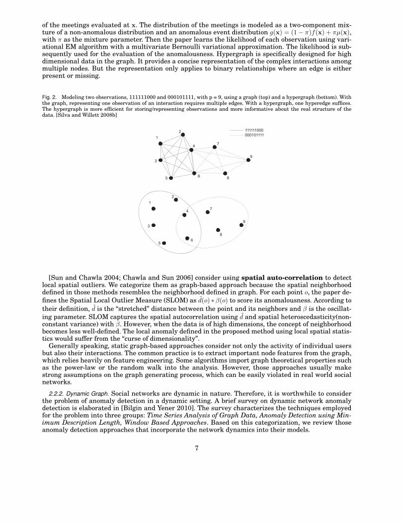
of the meetings evaluated at x. The distribution of the meetings is modeled as a two-component mix-ture of a non-anomalous distribution and an anomalous event distribution g(x) = (1− π)f(x) + πµ(x),with π as the mixture parameter. Then the paper learns the likelihood of each observation using vari-ational EM algorithm with a multivariate Bernoulli variational approximation. The likelihood is sub-sequently used for the evaluation of the anomalousness. Hypergraph is specifically designed for highdimensional data in the graph. It provides a concise representation of the complex interactions amongmultiple nodes. But the representation only applies to binary relationships where an edge is eitherpresent or missing.

Fig. 2. Modeling two observations, 111111000 and 000101111, with p = 9, using a graph (top) and a hypergraph (bottom). Withthe graph, representing one observation of an interaction requires multiple edges. With a hypergraph, one hyperedge suffices.The hypergraph is more efficient for storing/representing observations and more informative about the real structure of thedata. [Silva and Willett 2008b] 3

1

65

4

3

2

9

8

7

1

65

4

3

2

9

8

7

111111000000101111

Fig. 1

MODELING TWO OBSERVATIONS, 111111000 AND 000101111, WITH p = 9, USING A GRAPH (TOP) AND A HYPERGRAPH

(BOTTOM). WITH THE GRAPH, REPRESENTING ONE OBSERVATION OF AN INTERACTION REQUIRES MULTIPLE EDGES. WITH

A HYPERGRAPH, ONE HYPEREDGE SUFFICES. THE HYPERGRAPH IS MORE EFFICIENT FOR STORING/REPRESENTING

OBSERVATIONS AND MORE INFORMATIVE ABOUT THE REAL STRUCTURE OF THE DATA.

II. ANOMALY DETECTION ON HYPERGRAPHS

Let H = V , E be a hypergraph [7] with vertex set V and hyperedge set E . Each hyperedge,denoted x 2 E , can be represented as a binary string of length p. Bits set to 1 correspond tovertices that participate in the hyperedge. In this setting, we may approximately equate E with0, 1p, i.e. the binary hypercube of dimension p. (We say “approximately” due to the existenceof prohibited hyperedges, namely the origin, x = 0, and all x within Hamming distance 1 of theorigin, which correspond to interactions between zero or one network nodes. The impact of thisprecluded set becomes negligible for very large p and is omitted from this paper for simplicityof presentation.) This is a finite set with 2p elements. We define g(x) to be the probability massfunction (pmf) over E , evaluated at x.

Hypergraphs provide a more natural representation than graphs for multiple co-occurrence dataof the type examined in this paper. For example, one could consider using a graph to representco-occurrence data by having each vertex represent a network node and using weighted edges toconnect vertices associated with observed co-occurrences. As Figure 1 illustrates, using a graphin this manner would imply connecting any pair of vertices appearing in an observation with anedge. The edge structure of a graph is usually represented as a pp symmetric adjacency matrixwith p

2(p1) distinct elements, so that even converting observations into a collection edge weights

could be enormously challenging computationally. As Figure 1 illustrates, two observations can

[Sun and Chawla 2004; Chawla and Sun 2006] consider using spatial auto-correlation to detectlocal spatial outliers. We categorize them as graph-based approach because the spatial neighborhooddefined in those methods resembles the neighborhood defined in graph. For each point o, the paper de-fines the Spatial Local Outlier Measure (SLOM) as d(o) ∗ β(o) to score its anomalousness. According totheir definition, d is the “stretched” distance between the point and its neighbors and β is the oscillat-ing parameter. SLOM captures the spatial autocorrelation using d and spatial heteroscedasticity(non-constant variance) with β. However, when the data is of high dimensions, the concept of neighborhoodbecomes less well-defined. The local anomaly defined in the proposed method using local spatial statis-tics would suffer from the “curse of dimensionality”.

Generally speaking, static graph-based approaches consider not only the activity of individual usersbut also their interactions. The common practice is to extract important node features from the graph,which relies heavily on feature engineering. Some algorithms import graph theoretical properties suchas the power-law or the random walk into the analysis. However, those approaches usually makestrong assumptions on the graph generating process, which can be easily violated in real world socialnetworks.

2.2.2. Dynamic Graph. Social networks are dynamic in nature. Therefore, it is worthwhile to considerthe problem of anomaly detection in a dynamic setting. A brief survey on dynamic network anomalydetection is elaborated in [Bilgin and Yener 2010]. The survey characterizes the techniques employedfor the problem into three groups: Time Series Analysis of Graph Data, Anomaly Detection using Min-imum Description Length, Window Based Approaches. Based on this categorization, we review thoseanomaly detection approaches that incorporate the network dynamics into their models.

7

Dynamic networks can be represented as a time series of graphs. A common practice is to constructa time series from the graph observations or substructures. [Pincombe 2005] uses a number of graphtopology distance measures to quantify the differences between two consecutive networks, such asweight, edge, vertex, and diameter. For each of these graph topology distance measures, a time seriesof changes is constructed by comparing the graph for a given period with the graph(s) from one ormore previous periods. Given a graph G = V,E,WV ,WE, the algorithm constructs a time series ofchanges for each graph topology distance measures. Each time series is individually modeled by anARMA process. The anomaly is defined as days with residuals of more than two standard errorsfrom the best ARMA model. The paper detects anomalies by setting up a residual threshold for thegoodness of model fitting for time series. The proposed method in [Pincombe 2005] is designed forchange point detection. The performance of the proposed algorithm highly depends on how the graphtopology distance measures are defined. Additionally, the distance measure is only able to capture thecorrelation between two consecutive time stamps rather than long-range dependencies.

Graph eigenvectors of the adjacency matrices is another form of the time series extracted fromdynamic graph streams. In [Ide and Kashima 2004], the paper addresses the problem of anomalydetection in computer systems. Assume a system has N services, the paper defines a time evolvingdependency matrix D ∈ RN×N , where each element of the matrix Di,j is a function value relate to thenumber of service i’s requests for service j within a pre-determined time interval. Given a time series ofdependency matricesD(t), the algorithm extracts the principal eigenvector u(t) ofD(t) as the “activity”vector, which can be interpreted as the distribution of the probability that a service is holding thecontrol token of the system at a virtual time point. To detect anomalies, the authors define the typicalpattern as a linear combination of the past activity vectors r(t) = c

∑i=1Wviu(t− i+1), where vi are

the coefficients and c is the normalization constant. Then the algorithm calculates the dissimilarityof the present activity vector from this typical pattern. The anomaly metric z(t) is defined as z(t) =1− r(t− 1)Tu(t). When the anomaly metric quantity z(t) is greater than a given threshold, the systemflags anomalous situation. Compared with representing graphs with edges, weights and vertices as in[Pincombe 2005], features built upon eigenvectors capture the underlying invariant characteristics ofthe system and preserve good properties such as positivity, non-degeneracy, etc.

Besides time series analysis of the graph stream, Minimum description length (MDL) has beenapplied to anomaly detection as another way of characterizing the dynamic networks. [Sun et al. 2007]detects the change points in a stream of graph series. It introduces the concept of graph segment,which is one or more graph snapshots and the concept of source/destination partitions, which groupsthe source and destination nodes into clusters. Figure 3 illustrates those concepts in a three graphseries. The rational behind the algorithm is to consider whether it is easier to include a new graph intothe current graph segment or to start a new graph segment. If a new graph segment is created, it istreated as a change point. Given current graph segment G(s), encoding cost co and a new graph G(t),the algorithm computes the encoding cost for G(s) ⋃G(t) as cn and G(t) as c. If cn − co < c, the newgraph is included in the current segment. Otherwise, G(t) forms a new stream segment and time tis a change point. To compute the encoding cost of a graph segment, the algorithm tries to partitionthe nodes in a segment into source and destination nodes so that the MDL for encoding the partitionsis minimized. In this case, a change point indicates the time when the structure of the graph hasdramatically changed. One limitation of this algorithm is that it can only handle unweighted graphs,which cannot encode the intensity of the communication between users. Thus, this method does notfit the situation when the communications of people suddenly increase while the topological structurestays unchanged. (e.g. a heated discussion starting to prevail in a social network).

[Akoglu et al. 2012] addresses the categorical anomaly detection by pattern-based compression,which also adopts MDL-principle. It encodes a database with multiple code tables and searches forthe best partitioning of features using MDL-optimal rule. With the natural property of code tables, thealgorithm declares the anomaly by the pattern that has long code word, which are rarely used andhave high compression cost. The method has been successfully generalized to a broad range of data.The use of multiple code tables to describe the data in the proposed algorithm exploits the correlationsbetween groups of features. But the partition of the features into groups would impose unrealisticindependence assumptions on the data.

For window-based approach, scan statistics is the main-stream method. The idea of scan statisticsis to slide a small window over local regions, computing certain local statistic (number of events fora point pattern, or average pixel value for an image) for each window. The supremum or maximum

8

Fig. 3. A graph stream with 3 graphs in 2 segments. First graph segment consisting of G(1) and G(2) has two source partitionsI(1)1 = 1, 2, I(1)2 = 3, 4; two destination partitions J

(1)1 = 1, J(1) =2= 2, 3. Second graph segment consisting of G(3) has

three source partitions I(2)1 = 1, I(2)2 = 2, 3, I(2)3 = 4; three destination partitions J

(2)1 = 1, J(2)

2 = 2, J(2)3 = 3.

[Sun et al. 2007]

Figure 2: Notation illustration: A graph stream with 3

graphs in 2 segments. First graph segment consisting

of G(1) and G(2) has two source partitions I(1)1 = 1, 2,

I(1)2 = 3, 4; two destination partitions J

(1)1 = 1, J

(1)2 =

2, 3. Second graph segment consisting of G(3) has three

source partitions I(2)1 = 1, I

(2)2 = 2, 3, I

(2)3 = 4; three

destination partitions J(2)1 = 1, J

(2)2 = 2, J

(2)2 = 3.

is between (i) the number of bits needed to describe thecommunities (or, partitions) and their change points (or,segments) and (ii) the number of bits needed to describethe individual edges in the stream, given this information.

We begin by first assuming that the change-points as wellthe source and destination partitions for each graph seg-ment are given, and we show how to estimate the bit costto describe the individual edges (part (ii) above). Next, weshow how to incorporate the partitions and segments intoan encoding of the entire stream (part (i) above).

4.1 Graph encodingIn this paper, a graph is presented as a m-by-n binary

matrix. For example in Figure 2, G(1) is represented as

G(1) =

0

BB@

1 0 01 0 00 1 10 0 1

1

CCA (1)

Conceptually, we can store a given binary matrix as a bi-nary string with length mn, along with the two integers mand n. For example, equation 1 can be stored as 1100 0010 0011(in column major order), along with two integers 4 and 3.

To further save space, we can adopt some standard losslesscompression scheme (such as Human coding, or arithmeticcoding [8]) to encode the binary string, which formally canbe viewed as a sequence of realizations of a binomial randomvariable X. The code length for that is accurately estimatedas mnH(X) where H(X) is the entropy of variable X. For

notational convenience, we also write that as mnH(G(t)).Additionally, three integers need to be stored: the matrixsizes m and n, and the number of ones in the matrix (i.e.,the number of edges in the graph) denoted as |E| 1. The

1|E| is needed for computing the probability of ones or ze-ros, which is required for several encoding scheme such asHuman coding

cost for storing three integers is log|E|+logm+logn bits,where logis the universal code length for an integer2. Noticethat this scheme can be extended to a sequence of graphs ina segment.

More generally, if the random variable X can take valuesfrom the set M , with size |M | (a multinomial distribution),the entropy of X is

H(X) = PxM p(x) log p(x).

where p(x) is the probability that X = x. Moreover, themaximum of H(X) is log |M | when p(x)= 1

|M| for all x M

(pure random, most dicult to compress); the minimum is0 when p(x) = 1 for a particular x M (deterministic andconstant, easiest to compress). For the binomial case, if allsymbols are all 0 or all 1 in the string, we do not have tostore anything because by knowing the number of ones inthe string and the sizes of matrix, the receiver is alreadyable to decode the data completely.

With this observation in mind, the goal is to organize thematrix (graph) into some homogeneous sub-matrices withlow entropy and compress them separately, as we will de-scribe next.

4.2 Graph Segment encodingGiven a graph stream segment G(s) and its partition as-

signments, we can precisely compute the cost for transmit-ting the segment as two parts: 1) Partition encoding cost:the model complexity for partition assignments, 2) Graphencoding cost: the actual code for the graph segment.

Partition encoding costThe description complexity for transmitting the partitionassignments for graph segment G(s) consists of the followingterms:

First, we need to send the number of source and destina-tion nodes m and n using logm+logn bits. Note that, thisterm is constant, which has no eect on the choice of finalpartitions.

Second, we shall send the number of source and destina-tion partitions which is logks + logs.

Third, we shall send the source and destination partitionassignments. To exploit the non-uniformity across parti-tions, the encoding cost is mH(P ) + nH(Q) where P is a

multinomial random variable with the probability pi =m

(s)i

m

and m(s)i is the size of i-th source partition 1 i ks).

Similarly, Q is another multinomial random variable with

qi =n(s)in

and n(s)i is the size of i-th destination partition,

1 i s.For example in Figure 2, the partition sizes for first seg-

ment G(1) are m(1)1 = m

(1)2 = 2, n

(1)1 = 1, and n

(1)2 = 2; the

partition assignments for G(1) costs 4( 24

log( 24)+ 2

4log( 2

4))

3( 13

log( 13) + 2

3log( 2

3)) bits.

In summary, the partition encoding cost for graph seg-ment G(s) is

C(s)p := logm + logn + logks + logs + (2)

mH(P ) + nH(Q)

2To encode a positive integer x, we need logx log2 x +log2 log2 x + . . ., where only the positive terms are retainedand this is the optimal length, if the range of x is un-known [19]

690

Research Track Paper

of these locality statistics is known as the scan statistic. [Priebe et al. 2005] specifically discussesa framework of using scan statistics to perform anomaly detection on dynamic graphs. Specifically,the algorithm defines the scan region by considering the closed kth-order neighborhood of vertex v ingraph D = (V,E): Nk[v;D] = w ∈ V (D) : d(v, w) ≤ k. Here distance d(v, w) is the minimum directedpath length from v to w in D. The induced subdigraph Ω(N)(Nk[v;D]) is thus the scan region and anydigraph invariant Ψk(v) of the scan region is the locality statistics. For instance, the out degree of thedigraph can be one such invariant locality statistics. The scan statistic Mk(D) is the maximum localitystatistic over all vertices. The algorithm applies hypothesis testing by stating the null hypothesis(normality) and the alternative hypothesis (anomaly). Digraphs with large scan statistic indicatesthe existence of the anomalous activity and are rejected under null hypothesis with certain threshold.Extension of scan statistics from standard graph to hypergraph representation is also examined in[Park et al. 2008] for time-evolving graphs. The scan statistic is an intuitively appealing method toevaluate dynamic graph patterns. But one drawback of this type of method is the necessity to pre-specify a window width before one looks at the data.

3. GROUP ANOMALY DETECTIONGroup anomaly or “collective anomaly” detection in social network aims to discover groups of partic-ipants that collectively behave anomalously [Chandola et al. 2007]. This is a challenging task due tothree reasons: (1) we do not know beforehand any members of a malicious group; (2) the members ofanomalous groups may change over time; (3) usually no anomaly can be detected when we examineindividual member. Most existing algorithms can only address one or two of these challenges.

3.1. Activity-based Group Anomaly DetectionActivity-based group anomaly detection approaches usually assume that the group information isgiven beforehand and devote the most effort to model the activities within groups. Those approachesalso imply that groups are marginal independent with each other.

[Das et al. 2008] proposes a probabilistic model to detect group of anomalies in categorical data sets.It generalizes the spatial scan statistic in [Priebe et al. 2005] for dynamic graphs to non-spatial datasets with discrete valued attributes. It uses Bayesian networks to model the relationship between theattributes and computes the group score for all subsets of the data S based on the model likelihood:F (S) = P (Data|H1(S)

P (Data|H0). Under this definition, H0 is the null hypothesis that no anomalies are present,

and H1(S) is the alternative hypothesis specifying subset S is an anomalous group. Then it performsa heuristic search over arbitrary subsets of the data to find the groups that maximize the likelihood.

9

At the final stage, it performs randomization testing to evaluate the statistical significance of thedetected groups. For spatial data, the computation of scan statistics involves a definition of scanningregion, which is often based on geographical properties. Non-spatial categorical data has the difficultyin defining local statistics based on geographical properties. Therefore, the efficient search heuristic iscritical to the performance of algorithm. On the other hand, it lacks the solid theoretical justificationand is sensitive to model mis-specification.

[Das et al. 2009] considers the anomalies in categorical data sets and tries to detect anoma-lous attributes or combinations of attributes. The paper proposes two algorithms to test for anoma-lous records, i.e Conditional Probability Test and Marginal Probability Test. Conditional probabil-ity test uses conditional probability as the testing statistic. For two attributes at, bt, the algorithmconsiders the ration r(at, bt) = P (at)P (bt)

P (at,bt). Marginal probability computes a quantity called the q-

value, which is the cumulative probability mass of all the attributes q-val(at) =∑x∈X P (x) where

X = x : P (x) ≤ P (at). Q-value is in parallel with the p-value. This approach concerns with empiricaldistribution functions and is parameter free. But the underlying distributions of the attributes wouldheavily depend on the sample size of the data.

Another line of work formulates the group anomaly detection problem as a density estimationtask. It imposes a hierarchical probabilistic model on the normal groups and estimates the distributionof the latent variables in the model. It evaluates the likelihood of the estimated latent variables forindividual group and use it as a test statistic. The Multinomial Genre Model (MGM) proposed in [Xionget al. 2011b] first investigates the problem following the paradigm of latent models. MGM modelsgroups as a mixture of Gaussian distributions with different mixture rates. Formally, given M groups,each of which has Nm objects. MGM assumes that the object features Xm.n are generated from amixture of K Gaussian, m = 1, 2, · · · ,M , n = 1, 2, · · · , Nm with a set of stereotypical mixture ratesχ. The mixture rates of the M groups belong to one of the stereotypical mixture rates in χ. Figure 4depicts the graphical model of the proposed model. The method then performs Bayesian inference toestimate the density of the mixture rate for each group. Then group anomaly detection is conductedby scoring the mixture rate likelihood of each group. This method finds groups whose topic variablesZm, n are not compatible with any of the stereo- typical topic distributions in χ. In MGM, groupsshare the candidate topics β globally, which leads to bad performance when groups have differentsets of topics. [Xiong et al. 2011a] further extends MGM to Flexible Genre Model (FGM) with moreflexibility in the generation of topic distributions, as shown in Figure 4. The motivation of FGM isto allow each group to have its own topics. Specifically, they change the set of topics β from modelhyper-parameters to random variables, depending on the genre parameter η. This extension enablesthe model to adapt to more diverse genres in groups.

Apart from the generative approach used in MGM and FGM, [Muandet and Scholkopf 2013] takesa discriminative approach to estimate the density of the mixture model. It uses the same definitionof group anomaly from [Xiong et al. 2011b] and represents groups as probability distributions. Theauthors consider kernel embedding of those probabilistic distributions. For two probabilities P1 andP2, the kernel on probability distributions is defined as K(P1,P2) =

∫ ∫k(x, y)dPi(x)dPj(y), where k is

a reproducing kernel in reproducing kernel Hilbert space (RKHS). They generalize the technique ofone-class support vector machine (OCSVM) for point anomaly detection to group anomaly detection.Similar to OCSVM with translation invariant kernels, the authors compute the kernel of Gaussiandistributions and apply SVM in a probability measure space. Interestingly, the proposed one classsupport measure machine (OCSMM) algorithm has inherent correspondence to the kernel densityestimation, which is theoretically more attractive. Compared with generative approaches in [Xionget al. 2011b; Xiong et al. 2011a], OCSMM does not make assumptions on the underlying distributionof the data and is generally less computational expensive. However, due to the use of Gaussian RBFkernels and support vector machine, the algorithm is inevitably sensitive to the selection of kernels aswell as the soft margin parameter.

[Babbar et al. 2013] takes a casual approach to detect the contextual anomaly. The paper proposesto encode the variables in the Bayesian network and use probabilistic association rule to discoveranomalies. The association rule builds upon two measures namely support and confidence. Supportdescribes the prior probability of a variable while confidence represents the conditional probabil-ity. Given a state variable X and observations Y , the paper defines the two measures as followssuppport(X = xi) = P (X = xi) and confidence(X = xi) = Pa(X = xi|Y ), where Pa is the parentnodes of X in the Bayesian network. The algorithm detects the domain specific anomalous patterns

10

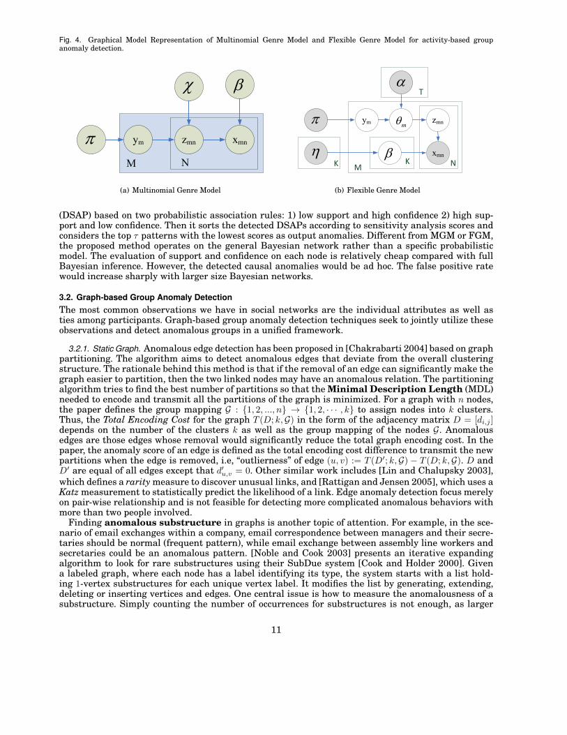
Fig. 4. Graphical Model Representation of Multinomial Genre Model and Flexible Genre Model for activity-based groupanomaly detection.

Liang Xiong, Barnabas Poczos, Jeff Schneider

think of these objects as ‘red’, ‘blue’, and ‘emissive’galaxies, and each group Gm is a set of Nm objects,each object can be one of the K different types. Intro-duce the SK = s ∈ RK |sk ≥ 0,

∑Kk=1 sk = 1 nota-

tion for the K-dimensional probability simplex, and letχt ∈ SK for all t = 1, . . . , T , and χ = χ1, . . . , χT de-note the set of T possible non-anomalous distributions(proportions) of the K different objects (red, blue, andemissive galaxies) in the M groups.

Now we can ask the question whether in group Gm thedistribution of these red, blue, and emissive galaxieslooks normal, that is, they look similar to a distribu-tion in χ = χ1, . . . , χT , or we have found a group,where this distribution seems far from the distribu-tions that we can see in the other groups.

In the following sections we will propose two generativeprobabilistic models that can help us to answer thisquestion and detect anomalous groups.

4 The Hierarchical Models

In this section we introduce our generative models thatdescribe the normal, that is the non-anomalous data,and then we show how we can detect anomalous groupsusing these models. Our proposed models are inspiredby the LDA, however, there are very significant differ-ences that we will explain later.

4.1 The Uni-Modal Model

The LDA model is a generative probabilistic modeloriginally proposed for modeling text corpora. Firstwe briefly review this model, and then explain howwe can extend this discrete model to be able to findanomalous groups in a data set given by any realvector-valued feature representation.

In the original LDA model the data set is a text corpus,that is a collection of M documents. Each documentGm is a set of Nm words, and each document is repre-sented by a random mixture over latent topics, which ischaracterized by a distribution over words. Formally,let Dir(π) denote the Dirichlet distribution with pa-rameter π, and let M(θ) be the multinomial distri-bution with parameters θ ∈ SK . In the LDA modelgiven some nonnegative hyperparameters π ∈ RK

+ , wegenerate first some θm ∈ SK (m = 1, . . . , M) from theDir(π) distribution (θm ∼ Dir(π)). Having these Kdimensional θm vectors (topic distributions) we gener-ate Zm,n ∼ M(θm) variables (n = 1, . . . , Nm) indicat-ing which topic is active out of K when we generatethe word Xm,n ∼ P (·|Zm,n, β). Here β = β1, . . . , βKis a dictionary of K f -dimensional probability vectors(βk ∈ Sf ), and P (·|Zm,n, β) = M(βZm,n

) is a multino-mial distribution with parameters βZm,n . While this

model has been shown to be very successful for mod-eling discrete data, such as text corpora, in its originalform it cannot be used for modeling real, vector-valuedobservations. Thus we modify this model slightly. In-stead of using M(βZm,n) for the observations, we as-sume βi = βµ

i , βΣi to be a mean value (βµ

i ∈ Rf )and a covariance matrix (βΣ

i ∈ Rf×f ), and our obser-vations are given by:

Xm,n ∼ P (·|Zm,n, β) = N (βµZm,n

, βΣZm,n

).

We call this model Gaussian-LDA (GLDA).

With GLDA we can model real, vector-valued obser-vations, but it has a serious problem when we want toapply it for group anomaly detection. GLDA learnsthat each group is a certain mixture of K Gaussiancomponents, but it also assumes that there is only one“best” mixture (topic distribution) for all groups, be-cause Dir(π), the distribution of topic distributionsθ ∈ SK , is uni-modal i.e. it peaks at a single point.While this is acceptable when used as the prior inLDA, it is too restrictive when used to model multi-modal distributions of topic distributions. To addressthis issue we extend the GLDA model with the previ-ously mentioned χ term, the set of the typical topic dis-tributions (proportions of the Gaussian components).

4.2 The Multi-Modal Model

In this section we introduce the Mixture of GaussianMixture Model (MGMM) model that extends GLDAwith a set of typical topic mixtures/distributions,and hence can resolve the previously mentioned uni-modality problem. The graphical representation ofthis new model can be seen in Figure 1.

xmnzmn

E

NM

ymS

F

Figure 1: The MGMM Model

Let again χt ∈ SK for all t = 1, . . . , T , and χ =χ1, . . . , χT denote the set of possible non-anomalousprobability distributions of the K different topics (red,blue, and emissive galaxies) in the M groups. Letπ ∈ ST denote a distribution vector on the set χ, andlet β = βµ

k , βΣk K

k=1 be a dictionary of the possiblemean values and covariance matrices.

The generative process of the MGMM model is de-scribed in Algorithm 1. Note that this model is differ-

(a) Multinomial Genre Model

xmn

zmn

ENM

ymS

D

mT

KK

T

K

Figure 1: The Flexible Genre Model (FGM).

global distributions P (·|). Thus, the topics can be adapted to local group data, but the informationis still shared globally. Moreover, the topic generators P (·|) determine how the topics m,kshould look like. In turn, if a group uses unusual topics to generate its points, it can be identified.

To handle real-valued multidimensional data, we set the point-generating distributions (i.e., the top-ics) to be Gaussians, P (xm,n|m,k) = N (xm,n|m,k), where m,k = µm,k,m,k includesthe mean and covariance parameters. For computational convenience, the topic generators areGaussian-Inverse-Wishart (GIW) distributions, which are conjugate to the Gaussian topics. Hencek = µ0,0, 0, 0 parameterizes the GIW distribution [17] (See the supplementary materialsfor more details). Let = ,↵, denote the model parameters. We can write the completelikelihood of data and latent variables in group Gm under FGM as follows:

P (Gm, ym, m,m|)

= M(ym|)Dir(m|↵ym)Y

kGIW (m,k|k)

Yn

M(zmn|m)N (xmn|m,zmn).

By integrating out m,m and summing out ym, z, we get the marginal likelihood of Gm:

P (Gm|) =X

t

t

Z

m,m

Dir(m|↵t)Y

k

GIW (m,k|k)Y

n

X

k

mkN (xmn|m,k)dmdm.

Finally, the data-set’s likelihood is just the product of all groups’ likelihoods.

4 Inference and Learning

To learn FGM, we update the parameters to maximize the likelihood of data. The inferred latentstates—including the topic distributions m, the topics m, and the topic and genre membershipszm, ym—can be used for detecting anomalies and exploring the data. Nonetheless, the inferenceand learning in FGM is intractable, so we train FGM using an approximate method described below.

4.1 Inference

The approximate inference of the latent variables can be done using Gibbs sampling [11]. In Gibbssampling, we iteratively update one variable at a time by drawing samples from its conditionaldistribution when all the other parameters are fixed. Thanks to the use of conjugate distributions,Gibbs sampling in FGM is simple and easy to implement. The sampling distributions of the latentvariables in group m are given below. We use P (·| ) to denote the distribution of one variableconditioned on all the others. For the genre membership ym we have that:

P (ym = t| ) / P (m|↵t)P (ym = t|) = tDir(m|↵t).

For the topic distribution m:

P (m| ) / P (zm|m)P (m|↵, ym) = M(zm|m)Dir(m|↵ym) = Dir(↵ym + nm),

where nm denotes the histogram of the K values in vector zm. The last equation follows from theDirichlet-Multinomial conjugacy. For m,k, the kth topic in group m, one can find that:

P (m,k| ) / P (x(k)m |m,k)P (m,k|k) = N (x(k)

m |m,k)GIW (m,k|k) = GIW (m,k|0k),

4

(b) Flexible Genre Model

(DSAP) based on two probabilistic association rules: 1) low support and high confidence 2) high sup-port and low confidence. Then it sorts the detected DSAPs according to sensitivity analysis scores andconsiders the top τ patterns with the lowest scores as output anomalies. Different from MGM or FGM,the proposed method operates on the general Bayesian network rather than a specific probabilisticmodel. The evaluation of support and confidence on each node is relatively cheap compared with fullBayesian inference. However, the detected causal anomalies would be ad hoc. The false positive ratewould increase sharply with larger size Bayesian networks.

3.2. Graph-based Group Anomaly DetectionThe most common observations we have in social networks are the individual attributes as well asties among participants. Graph-based group anomaly detection techniques seek to jointly utilize theseobservations and detect anomalous groups in a unified framework.

3.2.1. Static Graph. Anomalous edge detection has been proposed in [Chakrabarti 2004] based on graphpartitioning. The algorithm aims to detect anomalous edges that deviate from the overall clusteringstructure. The rationale behind this method is that if the removal of an edge can significantly make thegraph easier to partition, then the two linked nodes may have an anomalous relation. The partitioningalgorithm tries to find the best number of partitions so that the Minimal Description Length (MDL)needed to encode and transmit all the partitions of the graph is minimized. For a graph with n nodes,the paper defines the group mapping G : 1, 2, ..., n → 1, 2, · · · , k to assign nodes into k clusters.Thus, the Total Encoding Cost for the graph T (D; k,G) in the form of the adjacency matrix D = [di,j ]depends on the number of the clusters k as well as the group mapping of the nodes G. Anomalousedges are those edges whose removal would significantly reduce the total graph encoding cost. In thepaper, the anomaly score of an edge is defined as the total encoding cost difference to transmit the newpartitions when the edge is removed, i.e, “outlierness” of edge (u, v) := T (D′; k,G) − T (D; k,G). D andD′ are equal of all edges except that d′u,v = 0. Other similar work includes [Lin and Chalupsky 2003],which defines a rarity measure to discover unusual links, and [Rattigan and Jensen 2005], which uses aKatz measurement to statistically predict the likelihood of a link. Edge anomaly detection focus merelyon pair-wise relationship and is not feasible for detecting more complicated anomalous behaviors withmore than two people involved.

Finding anomalous substructure in graphs is another topic of attention. For example, in the sce-nario of email exchanges within a company, email correspondence between managers and their secre-taries should be normal (frequent pattern), while email exchange between assembly line workers andsecretaries could be an anomalous pattern. [Noble and Cook 2003] presents an iterative expandingalgorithm to look for rare substructures using their SubDue system [Cook and Holder 2000]. Givena labeled graph, where each node has a label identifying its type, the system starts with a list hold-ing 1-vertex substructures for each unique vertex label. It modifies the list by generating, extending,deleting or inserting vertices and edges. One central issue is how to measure the anomalousness of asubstructure. Simply counting the number of occurrences for substructures is not enough, as larger

11

substructures tend to have low occurrences. [Noble and Cook 2003] intuitively defines a score for asubstructure S in a graph G as F2 = Size(S) · Occurrences(S,G), which is simply the product of thetotal number of nodes within a substructure and its occurrences. A smaller value of F2 indicates amore abnormal substructure. Another issue of the problem is the computational complexity of the al-gorithm. Although [Cook and Holder 2000] shows that in practice the system runs in polynomial time,theoretically it faces exponential number of substructures.

The pioneering work of [Noble and Cook 2003] sees the rise of mining substructures in graphs.[Maruhashi et al. 2011] leverages the structural information in the heterogeneous networks to detectunusual subgraph patterns. The algorithm encodes the graph using a tensor and focuses on finding thesuspicious spikes via tensor decomposition. Formally, given an M-mode tensor X of size I1×I2×· · ·×IM , the algorithm performs CP decomposition of the tensor of rank R as X ≈∑R

r=1 λr(a(1)r × · · · a(M)

r ),where a(i)r are rank-1 eigenscore vectors. The approximation would be exact when R equals thetrue rank of the tensor. Next the algorithm transforms the eigenscore vector plot (absolute value ofeigenscore vs. attribute index) into the eigenscore histogram (absolute value of eigenscore vs. frequencycount) and conducts spike detection on the histogram. The proposed approaches bridges graph miningand tensor analysis. Tensor decomposition is able to capture the complex structure in heterogeneousnetworks. But tensor decomposition problem itself can be NP-hard to solve. And the lack of explicitobjective in the proposed anomaly detection framework would create difficulties in the final evaluationof the algorithm’s performance.

In the setting of fraudulent activity detection, [Eberle and Holder 2007] jointly considers anomaloussubstructure and the criteria of MDL. Specifically, they run the SUBDUE system with MDL heuris-tics to find the normative pattern in the graph. Instances of substructure are evaluated against thenormative pattern with a match cost. Anomalous substructures are the ones with the lowest matches.Based on this definition of group anomaly, [Eberle and Holder 2007] presents three slightly differentalgorithms, i.e. GBAD-MDL, GBAD-P and GBAD-MPS to detect anomalies. These methods first findall the instances of frequent substructures and evaluate the frequency of the abnormal structure mul-tiplied by the match cost. A key drawback of this method is that it assumes that the degree of nodesin a graph is uniformly distributed, which is almost impossible in most social networks. As shown in[McGlohon et al. 2008; Chakrabarti and Faloutsos 2006], real graphs usually follow power law degreedistribution instead of uniform distribution.

π p Gpaα Rpa Xpa

zp→q zp←q

Ypq

θm

βk

N ×N

M

ApN

K

B

In social media, two forms of data coexist: one is the point-wise data, which characterize the featuresof an individual person. The other is pair-wise relational data, which describe the properties of socialties. Density estimation methods for group anomaly detection [Xiong et al. 2011b; Xiong et al. 2011a;Muandet and Scholkopf 2013] emphasize on the point-wise data and usually overlook the pair-wiserelational data. Graph-based methods highlight the graph structure but usually fail to account forthe attributes of individual nodes. Additionally, existing group anomaly detections algorithms are alltwo-stage approaches: (i) identify groups, (ii) detect group anomalies. This strategy assumes that the

12

point-wise and pair-wise data are marginally independent. However, such independence assumptionmight underestimate the mutual influence between the group structure and the feature attributes.The detected group anomalies can hardly reveal the joint effect of these two forms of data.

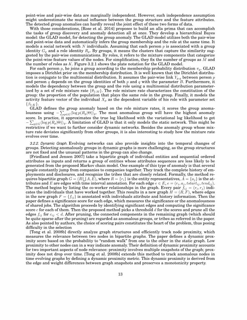
With those considerations, [Rose et al. 2014] proposes to build an alla prima that can accomplishthe tasks of group discovery and anomaly detection all at once. They develop a hierarchical Bayesmodel: the GLAD model, for detecting the group anomaly. The GLAD model utilizes both the pair-wiseand point-wise data and automatically infers the group membership and the role at the same time. Itmodels a social network with N individuals. Assuming that each person p is associated with a groupidentity Gp and a role identity Rp. By groups, it means the clusters that capture the similarity sug-gested by the pair-wise communications. By roles, it refers to the mixture components that categorizethe point-wise feature values of the nodes. For simplification, they fix the number of groups as M andthe number of roles as K. Figure 3.2.1 shows the plate notation for the GLAD model.

For each person p, he joins a group according to the membership probability distribution πp. GLADimposes a Dirichlet prior on the membership distribution. It is well known that the Dirichlet distribu-tion is conjugate to the multinomial distribution. It assumes the pair-wise link Yp,q between person pand person q depends on the group identities of both p and q with the parameter B. Furthermore, itmodels the dependency between the group and the role using a multinomial distribution parameter-ized by a set of role mixture rate θ1:M. The role mixture rate characterizes the constitution of thegroup: the proportion of the population that plays the same role in the group. Finally, it models theactivity feature vector of the individual Xp as the dependent variable of his role with parameter setβ1:K.

GLAD defines the group anomaly based on the role mixture rates, it scores the group anoma-lousness using −∑

p∈G〈log p(Rp|Θ)〉p. The most anomalous group will have the highest anomalyscore. In practice, it approximates the true log likelihood with the variational log likelihood to get−∑

p∈G〈log p(Rp|Θ)〉q. A limitation of GLAD is that it only models the static network. This might berestrictive if we want to further consider dynamic networks. Besides the anomaly group whose mix-ture rate deviates significantly from other groups, it is also interesting to study how the mixture rateevolves over time.

3.2.2. Dynamic Graph. Evolving networks can also provide insights into the temporal changes ofgroups. Detecting anomalously groups in dynamic graphs is more challenging, as the group structuresare not fixed and the unusual patterns in the group can also change.

[Friedland and Jensen 2007] take a bipartite graph of individual entities and sequential orderedattributes as inputs and returns a group of entities whose attributes sequences are less likely to begenerated from the proposed Markov chain model. One example of this type of anomaly is that severalpeople constantly jump from companies to companies together. They track the complete history of em-ployments and disclosures, and recognize the tribes that are closely related. Formally, the method re-quires bipartitie graph G = (R

⋃A,E), where R = ri is the entity representatives, A = aj is the at-

tributes and E are edges with time interval annotation. For each edge e ∈ E, e = (ri, aj , tstartij , tendij).The method begins by listing the co-worker relationships in the graph. Every pair fij = (ri, rj) indi-cates the individuals that have worked together. This results in a new graph H = (R,F ), where edgesin the new graph F = fij is annotated with individuals attribute and history information. Then thepaper defines a significance score for each edge, which measures the significance or the anomalousnessof shared jobs. The algorithm proceeds by identifying significant edges and computing the significancescore c for each of them. Then the proposed method picks a threshold d for the scores and prune all theedges fij for cij < d. After pruning, the connected components in the remaining graph (which shouldbe quite sparse after the pruning) are regarded as anomalous groups, or tribes as referred in the paper.As also pointed by authors, the choice of scoring pairs constitutes the heart of the problem, thus posingdifficulty in the selection

[Tong et al. 2008b] directly analyze graph structures and efficiently track node proximity, whichmeasures the relevance between two nodes in bipartite graphs. The paper defines a dynamic prox-imity score based on the probability to “random walk” from one to the other in the static graph. Lowproximity to other nodes can in a way indicate anomaly. Their definition of dynamic proximity accountsfor two important aspects of node relevance: proximity involves multiple snapshots of the graph; prox-imity does not drop over time. [Tong et al. 2008b] extends this method to track anomalous nodes intime evolving graphs by defining a dynamic proximity metric. This dynamic proximity is derived fromthe edge and weight differences between graph snapshots and preserves a monotonicity property.

13

[Liu et al. 2008] proposes to detect the significant changing subgraphs. Given two consecutivesnapshots of a graph Gi−1 and Gi, the algorithm defines an importance score to measure the ac-cumulative change of a node’s closeness to its l-step neighbors (neighbors within l hops from thenode) between two consecutive graph slices. In their context, random walk with restart is usedto model the node relevance. The closeness of a pair of vertices vj and vk is defined as Πl(j, k) =∑τ :vj=→vk;length(τ)≤l p(τ)c(1 − c)length(τ), where τ is a path from vj to vk whose length is length(τ) with

transition probability p(τ). The importance score is therefore the summation of the closeness changesof vj to the other nodes, defined as V Ii(vj) =

∑vk∈Vi

|Πli−1(j, k) − Πl

i(j, k)| . Note that two consecu-tive graph slices Gi and Gi+1 have the same set of nodes, but their edge set could be different. Withthe node closeness Πl

i and the vertex importance score V I, the paper uses a strategy similar to den-sity clustering to detect the significant subgraphs. Specifically, the algorithm puts the most importantnode in the current subgraph g, adds all of its l-step neighbors to a max-heap. As long as there existsa node whose closeness with node t exceeds certain threshold, the algorithm iteratively moves t fromthe heap into g. When the iteration terminates, g is regarded as the anomalous subgraph, and thealgorithm proceeds to generate anomalous subgraphs for the next timestamp. The proposed algorithmdetects subgraphs with significant change in edges as group anomalies. The incremental learning ofnodes closeness changes makes the algorithm quite efficiently. However, the output subgraphs heavilyrely on the threshold for the closeness, and there is no clear mapping between the nodes’ closeness andanomalousness.

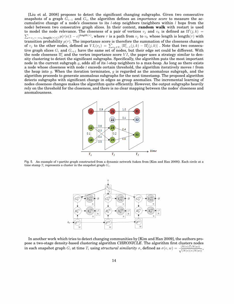
CHRONICLE: A Two-Stage Density-based Clustering of Dynamic Networks 3

works, it has also some weak points: (1) finding only stable clusters of singlepath (i.e., a sequence of local clusters over time); (2) finding a very small numberof clusters (i.e., the most stable top-k clusters); (3) not being scalable w.r.t. thelength of dynamic networks; and (4) using a large amount of memory dependingon its parameters. All these weak points are caused by the fact that the BFSmethod is based on a dynamic programming (DP) algorithm. Besides the clustersof single path type, actually, there are many cohesive clusters of non-single pathtype in t-partite graph. Figure 2 shows an example of t-partite graph over threetimestamp networks. Each network has 3∼4 local clusters. The numbers on linesbetween T1 and T2 (or T2 and T3) indicate that they have a non-zero similarity.When k = 1, the BFS method finds a single path cluster c11c21c31 because it hasthe strongest similarities between local clusters. However, if some members inc12 transfer to c24, some members in c13 to c23, and the members in c23 and c24are merged into c33, then there could be another cluster like (c12c13)(c23c24)c33,where the similarity between (c12c13) and (c23c24) and the similarity between(c23c24) and c33 might be very high (i.e., very cohesive) although the similarityof each single path (e.g., c13c23c33) are not so high. Here, () represents a consol-idation of multiple local clusters. We call a cluster of this type as a path groupcluster since there are multiple paths over time in the cluster. The BFS cannotfind the clusters of this type.

Fig. 2. An example of t-partite graph constructed from a dynamic network.

In this paper, we propose a density-based clustering algorithm, CHRONI-CLE, that efficiently discovers both single path clusters and path group clusters.For finding clusters of both types, CHRONICLE performs the density-basedclustering in two stages: the 1st-stage density-based clustering for each times-tamp network and the 2nd-stage density-based clustering for the t-partite graph.In case of the previous BFS method, it only performs the 1st-stage clusteringand finds single path clusters by using a DP algorithm. A density-based clus-tering approach has several advantages such as discovering clusters of arbitraryshape, handling noise, and being fast. These features allow us to find a widerrange of clusters (i.e., not only single path clusters, but also path group clusters)in an efficient way. As the length of dynamic networks, the number of clusters,or the length of cluster (i.e., path length) increases, the running time and theamount of memory usage of the BFS method largely increase. Using disk for sav-

Fig. 5. An example of t-partite graph constructed from a dynamic network (taken from [Kim and Han 2009]). Each circle at atime stamp Ti represents a cluster in the snapshot graph Gi.

G(1)p Y

(1)p,q

R(1)p X

(1)p

B

(1)0

G(2)p Y

(2)p,q

R(2)p X

(2)p

B

(2)

G(t)p Y

(t)p,q

R(t)p X

(t)p

B

(t)

p

↵

N

N

M

K

N

N

M

K

N

N

M

K

N

1

In another work which tries to detect changing communities by [Kim and Han 2009], the authors pro-pose a two-stage density-based clustering algorithm CHRONICLE. The algorithm first clusters nodesin each snapshot graph Gi at time Ti using structural similarity σ, defined as σ(v, w) = |N(v)

⋂N(w)|√

|N(v)|×|N(w)|,

14

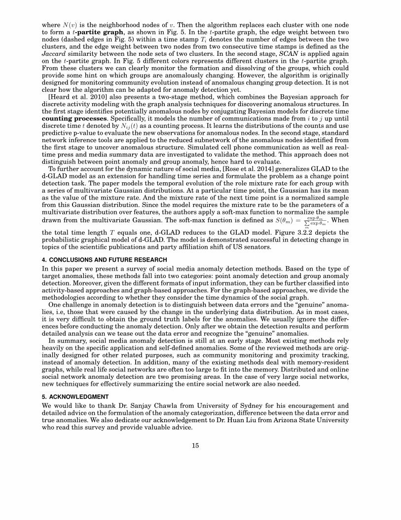
where N(v) is the neighborhood nodes of v. Then the algorithm replaces each cluster with one nodeto form a t-partite graph, as shown in Fig. 5. In the t-partite graph, the edge weight between twonodes (dashed edges in Fig. 5) within a time stamp Ti denotes the number of edges between the twoclusters, and the edge weight between two nodes from two consecutive time stamps is defined as theJaccard similarity between the node sets of two clusters. In the second stage, SCAN is applied againon the t-partite graph. In Fig. 5 different colors represents different clusters in the t-partite graph.From these clusters we can clearly monitor the formation and dissolving of the groups, which couldprovide some hint on which groups are anomalously changing. However, the algorithm is originallydesigned for monitoring community evolution instead of anomalous changing group detection. It is notclear how the algorithm can be adapted for anomaly detection yet.

[Heard et al. 2010] also presents a two-stage method, which combines the Bayesian approach fordiscrete activity modeling with the graph analysis techniques for discovering anomalous structures. Inthe first stage identifies potentially anomalous nodes by conjugating Bayesian models for discrete timecounting processes. Specifically, it models the number of communications made from i to j up untildiscrete time t denoted by Nij(t) as a counting process. It learns the distributions of the counts and usepredictive p-value to evaluate the new observations for anomalous nodes. In the second stage, standardnetwork inference tools are applied to the reduced subnetwork of the anomalous nodes identified fromthe first stage to uncover anomalous structure. Simulated cell phone communication as well as real-time press and media summary data are investigated to validate the method. This approach does notdistinguish between point anomaly and group anomaly, hence hard to evaluate.

To further account for the dynamic nature of social media, [Rose et al. 2014] generalizes GLAD to thed-GLAD model as an extension for handling time series and formulate the problem as a change pointdetection task. The paper models the temporal evolution of the role mixture rate for each group witha series of multivariate Gaussian distributions. At a particular time point, the Gaussian has its meanas the value of the mixture rate. And the mixture rate of the next time point is a normalized samplefrom this Gaussian distribution. Since the model requires the mixture rate to be the parameters of amultivariate distribution over features, the authors apply a soft-max function to normalize the sampledrawn from the multivariate Gaussian. The soft-max function is defined as S(θm) = exp θm∑

mexp θm

. When

the total time length T equals one, d-GLAD reduces to the GLAD model. Figure 3.2.2 depicts theprobabilistic graphical model of d-GLAD. The model is demonstrated successful in detecting change intopics of the scientific publications and party affiliation shift of US senators.

4. CONCLUSIONS AND FUTURE RESEARCHIn this paper we present a survey of social media anomaly detection methods. Based on the type oftarget anomalies, these methods fall into two categories: point anomaly detection and group anomalydetection. Moreover, given the different formats of input information, they can be further classified intoactivity-based approaches and graph-based approaches. For the graph-based approaches, we divide themethodologies according to whether they consider the time dynamics of the social graph.

One challenge in anomaly detection is to distinguish between data errors and the “genuine” anoma-lies, i.e, those that were caused by the change in the underlying data distribution. As in most cases,it is very difficult to obtain the ground truth labels for the anomalies. We usually ignore the differ-ences before conducting the anomaly detection. Only after we obtain the detection results and performdetailed analysis can we tease out the data error and recognize the “genuine” anomalies.

In summary, social media anomaly detection is still at an early stage. Most existing methods relyheavily on the specific application and self-defined anomalies. Some of the reviewed methods are orig-inally designed for other related purposes, such as community monitoring and proximity tracking,instead of anomaly detection. In addition, many of the existing methods deal with memory-residentgraphs, while real life social networks are often too large to fit into the memory. Distributed and onlinesocial network anomaly detection are two promising areas. In the case of very large social networks,new techniques for effectively summarizing the entire social network are also needed.

5. ACKNOWLEDGMENTWe would like to thank Dr. Sanjay Chawla from University of Sydney for his encouragement anddetailed advice on the formulation of the anomaly categorization, difference between the data error andtrue anomalies. We also dedicate our acknowledgement to Dr. Huan Liu from Arizona State Universitywho read this survey and provide valuable advice.

15

REFERENCESTarem Ahmed, Tarem Ahmed, Boris Oreshkin, and Mark” Coates. 2007. Machine learning approaches to network anomaly

detection. In Proceedings of the second workshop on tackling computer systems problems with machine learning(SYSML)(2007). DOI:http://dx.doi.org/8080/citeseerx/viewdoc/summary?doi=10.1.1.129.238

L Akoglu and M McGlohon. 2009. Anomaly detection in large graphs. In CMU-CS-09-173 Technical November (2009).Leman Akoglu, Mary McGlohon, and Christos Faloutsos. 2010. Oddball: Spotting anomalies in weighted graphs. In Advances in

Knowledge Discovery and Data Mining. Springer, 410–421.L. Akoglu, H. Tong, J. Vreeken, and C. Faloutsos. 2012. Fast and Reliable Anomaly Detection in Categorical Data. (2012).Sakshi Babbar, Didi Surian, and Sanjay Chawla. 2013. A Causal Approach for Mining Interesting Anomalies. In Advances in

Artificial Intelligence. Springer, 226–232.C.C. Bilgin and B. Yener. 2010. Dynamic network evolution: Models, clustering, anomaly detection. Technical Report. Technical

Report, 2008, Rensselaer University, NY.David M. Blei and John D. Lafferty. 2006. Dynamic topic models. In Proceedings of the 23rd international conference on Machine

learning (ICML ’06). ACM, New York, NY, USA, 113–120. DOI:http://dx.doi.org/10.1145/1143844.1143859David M. Blei, Andrew Y. Ng, and Michael I. Jordan. 2003. Latent dirichlet allocation. J. Mach. Learn. Res. 3 (March 2003),

993–1022.Deepayan Chakrabarti. 2004. AutoPart: parameter-free graph partitioning and outlier detection. In Proceedings of the 8th Eu-

ropean Conference on Principles and Practice of Knowledge Discovery in Databases (PKDD ’04). Springer-Verlag New York,Inc., New York, NY, USA, 112–124.

Deepayan Chakrabarti and Christos Faloutsos. 2006. Graph mining: Laws, generators, and algorithms. ACM Comput. Surv. 38,1, Article 2 (June 2006). DOI:http://dx.doi.org/10.1145/1132952.1132954

P.K. Chan and S.J. Stolfo. 1998. Toward scalable learning with non-uniform class and cost distributions: A case study in creditcard fraud detection.. In KDD’98. 164–168.

V. Chandola, A. Banerjee, and V. Kumar. 2007. Outlier detection: A survey. ACM Computing Surveys, to appear (2007).Varun Chandola, Arindam Banerjee, and Vipin Kumar. 2012. Anomaly Detection for Discrete Sequences: A Survey. IEEE Trans.

on Knowl. and Data Eng. 24, 5 (May 2012), 823–839. DOI:http://dx.doi.org/10.1109/TKDE.2010.235Varun Chandola, Varun Chandola, Arindam Banerjee, and Vipin” Kumar. 2007. Anomaly Detection: A Survey. (2007).

DOI:http://dx.doi.org/8080/citeseerx/viewdoc/summary?doi=10.1.1.155.3799Sanjay Chawla and Pei Sun. 2006. SLOM: a new measure for local spatial outliers. Knowledge and Information Systems 9, 4

(2006), 412–429.Haibin Cheng, Pang-Ning Tan, Christopher Potter, and Steven Klooster. 2009. Detection and characterization of anomalies in

multivariate time series.. In SDM’09. 413–424.Diane J. Cook and Lawrence B. Holder. 2000. Graph-Based Data Mining. IEEE Intelligent Systems 15, 2 (March 2000), 32–41.

DOI:http://dx.doi.org/10.1109/5254.850825K. Das, J. Schneider, and D.B. Neill. 2009. Detecting anomalous groups in categorical datasets. Carnegie Mellon University,

School of Computer Science, Machine Learning Department.Kaustav Das, Jeff Schneider, and Daniel B Neill. 2008. Anomaly pattern detection in categorical datasets. In Proceedings of the

14th ACM SIGKDD international conference on Knowledge discovery and data mining. ACM, 169–176.Florence Duchene, Catherine Garbay, and Vincent Rialle. 2004. Mining Heterogeneous Multivariate Time-Series for Learning

Meaningful Patterns: Application to Home Health Telecare. CoRR abs/cs/0412003 (2004).William Dumouchel. 1999. Computer Intrusion Detection Based on Bayes Factors for Comparing Command Transition Probabil-

ities. Technical Report.William Eberle and Lawrence Holder. 2007. Discovering Structural Anomalies in Graph-Based Data. In Proceedings of the

Seventh IEEE International Conference on Data Mining Workshops (ICDMW ’07). IEEE Computer Society, Washington, DC,USA, 393–398. DOI:http://dx.doi.org/10.1109/ICDMW.2007.35

Elena Erosheva, Stephen Fienberg, and John Lafferty. 2004. Mixed-membership models of scientific publications. Proceed-ings of the National Academy of Sciences of the United States of America 101, Suppl 1 (6 April 2004), 5220–5227.DOI:http://dx.doi.org/10.1073/pnas.0307760101

E. Eskin, A. Arnold, M. Prerau, L. Portnoy, and S. Stolfo. 2002. A geometric framework for unsupervised anomaly detection:Detecting intrusions in unlabeled data. Kluwer.

Lisa Friedland and David Jensen. 2007. Finding tribes: identifying close-knit individuals from employment patterns. In Pro-ceedings of the 13th ACM SIGKDD international conference on Knowledge discovery and data mining (KDD ’07). ACM, NewYork, NY, USA, 290–299. DOI:http://dx.doi.org/10.1145/1281192.1281226

Anup K. Ghosh and Aaron Schwartzbard. 1999. A study in using neural networks for anomaly and misuse detection. In Pro-ceedings of the 8th conference on USENIX Security Symposium - Volume 8 (SSYM’99). USENIX Association, Berkeley, CA,USA, 12–12.

Valery Guralnik and Jaideep Srivastava. 1999. Event detection from time series data. In Proceedings of the fifth ACMSIGKDD international conference on Knowledge discovery and data mining (KDD ’99). ACM, New York, NY, USA, 33–42.DOI:http://dx.doi.org/10.1145/312129.312190

Steve Hanneke and Eric P. Xing. 2007. Discrete temporal models of social networks. In Proceedings of the 2006 conference onStatistical network analysis (ICML’06). Springer-Verlag, Berlin, Heidelberg, 115–125.

D.M. Hawkins. 1980. Identification of outliers. Chapman and Hall.

16

Nicholas A. Heard, David J. Weston, Kiriaki Platanioti, and David J. Hand. 2010. Bayesian anomaly detection methods for socialnetworks. (11 2010).

C. Horn and R. Willett. 2011. Online anomaly detection with expert system feedback in social networks. In Acoustics, Speechand Signal Processing (ICASSP), 2011 IEEE International Conference on. IEEE, 1936–1939.

Tsuyoshi Ide and Hisashi Kashima. 2004. Eigenspace-based anomaly detection in computer systems. In Proceedings of the tenthACM SIGKDD international conference on Knowledge discovery and data mining. ACM, 440–449.

Alexander Ihler, Jon Hutchins, and Padhraic Smyth. 2006. Adaptive event detection with time-varying poisson processes. InProceedings of the 12th ACM SIGKDD international conference on Knowledge discovery and data mining (KDD ’06). ACM,New York, NY, USA, 207–216. DOI:http://dx.doi.org/10.1145/1150402.1150428

Wen H. Ju and Yehuda Vardi. 2001. A Hybrid High-Order Markov Chain Model for Computer Intrusion Detection. Journal ofComputational and Graphical Statistics 10, 2 (2001), 277–295. DOI:http://dx.doi.org/10.1198/10618600152628068

Eamonn Keogh, Jessica Lin, and Ada Fu. 2005. HOT SAX: Efficiently Finding the Most Unusual Time Series Subsequence. InProceedings of the Fifth IEEE International Conference on Data Mining (ICDM ’05). IEEE Computer Society, Washington,DC, USA, 226–233. DOI:http://dx.doi.org/10.1109/ICDM.2005.79

Min-Soo Kim and Jiawei Han. 2009. CHRONICLE: A Two-Stage Density-Based Clustering Algorithm for Dynamic Networks.In Proceedings of the 12th International Conference on Discovery Science (DS ’09). Springer-Verlag, Berlin, Heidelberg, 152–167. DOI:http://dx.doi.org/10.1007/978-3-642-04747-3 14

Jon M. Kleinberg. 1999. Authoritative sources in a hyperlinked environment. J. ACM 46, 5 (Sept. 1999), 604–632.DOI:http://dx.doi.org/10.1145/324133.324140

Mladen Kolar, Le Song, Amr Ahmed, and Eric P. Xing. 2010. Estimating time-varying networks. Annals of Applied Statistics 4,1 (2010), 94–123.

Anukool Lakhina, Mark Crovella, and Christophe Diot. 2004. Diagnosing network-wide traffic anomalies. SIGCOMM Comput.Commun. Rev. 34 (August 2004), 219–230. Issue 4. DOI:http://dx.doi.org/10.1145/1030194.1015492

Theodoros Lappas, Kun Liu, and Evimaria Terzi. 2009. Finding a team of experts in social networks. In Proceedings of the 15thACM SIGKDD international conference on Knowledge discovery and data mining (KDD ’09). ACM, New York, NY, USA,467–476. DOI:http://dx.doi.org/10.1145/1557019.1557074

Ar Lazarevic, Ar Lazarevic, Aysel Ozgur, Levent Ertoz, Jaideep Srivastava, and Vipin” Kumar. 2003. A comparative study ofanomaly detection schemes in network intrusion detection. In Proceedings of the third SIAM international conference onData Mining (2003). DOI:http://dx.doi.org/8080/citeseerx/viewdoc/summary?doi=10.1.1.91.2580

Jessica Lin, Eamonn Keogh, Stefano Lonardi, and Bill Chiu. 2003. A symbolic representation of time series, with implications forstreaming algorithms. In Proceedings of the 8th ACM SIGMOD workshop on Research issues in data mining and knowledgediscovery (DMKD ’03). ACM, New York, NY, USA, 2–11. DOI:http://dx.doi.org/10.1145/882082.882086

Shou-de Lin and Hans Chalupsky. 2003. Unsupervised Link Discovery in Multi-relational Data via Rarity Analysis. In Proceed-ings of the Third IEEE International Conference on Data Mining (ICDM ’03). IEEE Computer Society, Washington, DC,USA, 171–.

Zheng Liu, Jeffrey Xu Yu, Yiping Ke, Xuemin Lin, and Lei Chen. 2008. Spotting Significant Changing Subgraphs in EvolvingGraphs. In Proceedings of the 2008 Eighth IEEE International Conference on Data Mining (ICDM ’08). IEEE ComputerSociety, Washington, DC, USA, 917–922. DOI:http://dx.doi.org/10.1109/ICDM.2008.112

Ulrike Luxburg. 2007. A tutorial on spectral clustering. Statistics and Computing 17, 4 (Dec. 2007), 395–416.DOI:http://dx.doi.org/10.1007/s11222-007-9033-z

Koji Maruhashi, Fan Guo, and Christos Faloutsos. 2011. Multiaspectforensics: Pattern mining on large-scale heterogeneous net-works with tensor analysis. In Advances in Social Networks Analysis and Mining (ASONAM), 2011 International Conferenceon. IEEE, 203–210.

Mary McGlohon, Leman Akoglu, and Christos Faloutsos. 2008. Weighted graphs and disconnected components: patterns anda generator. In Proceedings of the 14th ACM SIGKDD international conference on Knowledge discovery and data mining(KDD ’08). ACM, New York, NY, USA, 524–532. DOI:http://dx.doi.org/10.1145/1401890.1401955

H. D. K. Moonesinghe and Pang-Ning Tan. 2008. Outrank: a Graph-Based Outlier Detection Framework Using Random Walk.International Journal on Artificial Intelligence Tools 17, 1 (2008).

Krikamol Muandet and Bernhard Scholkopf. 2013. One-class support measure machines for group anomaly detection. stat 1050(2013), 1.

C.C. Noble and D.J. Cook. 2003. Graph-based anomaly detection. In Proceedings of the ninth ACM SIGKDD international con-ference on Knowledge discovery and data mining. ACM, 631–636.

Jia-Yu Pan, Hyung-Jeong Yang, Christos Faloutsos, and Pinar Duygulu. 2004. Automatic multimedia cross-modal correlationdiscovery. In Proceedings of the tenth ACM SIGKDD international conference on Knowledge discovery and data mining (KDD’04). ACM, New York, NY, USA, 653–658. DOI:http://dx.doi.org/10.1145/1014052.1014135

DMY Park, C.E. Priebe, D.J. Marchette, and A. Youssef. 2008. Scan statistics on enron hypergraphs. Interface (2008).Brandon Pincombe. 2005. Anomaly Detection in Time Series of Graphs using ARMA Processes. ASOR BULLETIN 24, 4 (2005),

2.Carey E. Priebe, John M. Conroy, David J. Marchette, and Youngser Park. 2005. Scan Statistics on Enron Graphs. Comput.

Math. Organ. Theory 11, 3 (Oct. 2005), 229–247. DOI:http://dx.doi.org/10.1007/s10588-005-5378-zMatthew J. Rattigan and David Jensen. 2005. The case for anomalous link discovery. SIGKDD Explor. Newsl. 7, 2 (Dec. 2005),

41–47. DOI:http://dx.doi.org/10.1145/1117454.1117460

17

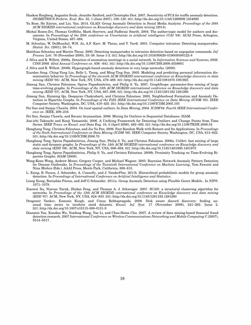
Haakon Ringberg, Augustin Soule, Jennifer Rexford, and Christophe Diot. 2007. Sensitivity of PCA for traffic anomaly detection.SIGMETRICS Perform. Eval. Rev. 35, 1 (June 2007), 109–120. DOI:http://dx.doi.org/10.1145/1269899.1254895

Yu Rose, He Xinran, and Liu. Yan. 2014. GLAD: Group Anomaly Detection in Social Media Analysis. Proceedings of the 20thACM SIGKDD international conference on Knowledge discovery and data mining (2014).

Michal Rosen-Zvi, Thomas Griffiths, Mark Steyvers, and Padhraic Smyth. 2004. The author-topic model for authors and doc-uments. In Proceedings of the 20th conference on Uncertainty in artificial intelligence (UAI ’04). AUAI Press, Arlington,Virginia, United States, 487–494.

M. Schonlau, W. DuMouchel, W.H. Ju, A.F. Karr, M. Theus, and Y. Vardi. 2001. Computer intrusion: Detecting masquerades.Statist. Sci. (2001), 58–74.

Matthias Schonlau and Martin Theus. 2000. Detecting masquerades in intrusion detection based on unpopular commands. Inf.Process. Lett. 76 (November 2000), 33–38. Issue 1-2. DOI:http://dx.doi.org/10.1016/S0020-0190(00)00122-8

J. Silva and R. Willett. 2008a. Detection of anomalous meetings in a social network. In Information Sciences and Systems, 2008.CISS 2008. 42nd Annual Conference on. 636 –641. DOI:http://dx.doi.org/10.1109/CISS.2008.4558601

J. Silva and R. Willett. 2008b. Hypergraph-based anomaly detection in very large networks. (2008).Xiaodan Song, Ching-Yung Lin, Belle L. Tseng, and Ming-Ting Sun. 2005. Modeling and predicting personal information dis-

semination behavior. In Proceedings of the eleventh ACM SIGKDD international conference on Knowledge discovery in datamining (KDD ’05). ACM, New York, NY, USA, 479–488. DOI:http://dx.doi.org/10.1145/1081870.1081925

Jimeng Sun, Christos Faloutsos, Spiros Papadimitriou, and Philip S. Yu. 2007. GraphScope: parameter-free mining of largetime-evolving graphs. In Proceedings of the 13th ACM SIGKDD international conference on Knowledge discovery and datamining (KDD ’07). ACM, New York, NY, USA, 687–696. DOI:http://dx.doi.org/10.1145/1281192.1281266

Jimeng Sun, Huiming Qu, Deepayan Chakrabarti, and Christos Faloutsos. 2005. Neighborhood Formation and Anomaly De-tection in Bipartite Graphs. In Proceedings of the Fifth IEEE International Conference on Data Mining (ICDM ’05). IEEEComputer Society, Washington, DC, USA, 418–425. DOI:http://dx.doi.org/10.1109/ICDM.2005.103

Pei Sun and Sanjay Chawla. 2004. On local spatial outliers. In Data Mining, 2004. ICDM’04. Fourth IEEE International Confer-ence on. IEEE, 209–216.

Pei Sun, Sanjay Chawla, and Bavani Arunasalam. 2006. Mining for Outliers in Sequential Databases. SIAM.Jun-ichi Takeuchi and Kenji Yamanishi. 2006. A Unifying Framework for Detecting Outliers and Change Points from Time

Series. IEEE Trans. on Knowl. and Data Eng. 18, 4 (April 2006), 482–492. DOI:http://dx.doi.org/10.1109/TKDE.2006.54Hanghang Tong, Christos Faloutsos, and Jia-Yu Pan. 2006. Fast Random Walk with Restart and Its Applications. In Proceedings

of the Sixth International Conference on Data Mining (ICDM ’06). IEEE Computer Society, Washington, DC, USA, 613–622.DOI:http://dx.doi.org/10.1109/ICDM.2006.70

Hanghang Tong, Spiros Papadimitriou, Jimeng Sun, Philip S. Yu, and Christos Faloutsos. 2008a. Colibri: fast mining of largestatic and dynamic graphs. In Proceedings of the 14th ACM SIGKDD international conference on Knowledge discovery anddata mining (KDD ’08). ACM, New York, NY, USA, 686–694. DOI:http://dx.doi.org/10.1145/1401890.1401973

Hanghang Tong, Spiros Papadimitriou, Philip S. Yu, and Christos Faloutsos. 2008b. Proximity Tracking on Time-Evolving Bi-partite Graphs. SIAM (2008).

Weng-Keen Wong, Andrew Moore, Gregory Cooper, and Michael Wagner. 2003. Bayesian Network Anomaly Pattern Detectionfor Disease Outbreaks. In Proceedings of the Twentieth International Conference on Machine Learning, Tom Fawcett andNina Mishra (Eds.). AAAI Press, Menlo Park, California, 808–815.

L. Xiong, B. Poczos, J. Schneider, A. Connolly, and J. VanderPlas. 2011b. Hierarchical probabilistic models for group anomalydetection. In Proceedings of International Conference on Artifcial Intelligence and Statistics.

Liang Xiong, Barnabas Poczos, and Jeff G Schneider. 2011a. Group Anomaly Detection using Flexible Genre Models.. In NIPS.1071–1079.

Xiaowei Xu, Nurcan Yuruk, Zhidan Feng, and Thomas A. J. Schweiger. 2007. SCAN: a structural clustering algorithm fornetworks. In Proceedings of the 13th ACM SIGKDD international conference on Knowledge discovery and data mining(KDD ’07). ACM, New York, NY, USA, 824–833. DOI:http://dx.doi.org/10.1145/1281192.1281280

Dragomir Yankov, Eamonn Keogh, and Umaa Rebbapragada. 2008. Disk aware discord discovery: finding un-usual time series in terabyte sized datasets. Knowl. Inf. Syst. 17 (November 2008), 241–262. Issue 2.DOI:http://dx.doi.org/10.1007/s10115-008-0131-9

Dianmin Yue, Xiaodan Wu, Yunfeng Wang, Yue Li, and Chao-Hsien Chu. 2007. A review of data mining-based financial frauddetection research. 2007 International Conference on Wireless Communications Networking and Mobile Computing C (2007),5514–5517.

18