A Theory of Capital Controls as

Dynamic Terms-of-Trade Manipulation∗

Arnaud Costinot

MIT, CEPR, and NBER

Guido Lorenzoni

Northwestern University and NBER

Iván Werning

MIT and NBER

August 2013

Abstract

We develop a theory of capital controls as dynamic terms-of-trade manipulation. We

study an infinite horizon endowment economy with two countries. One country

chooses taxes on international capital flows in order to maximize the welfare of its

representative agent, while the other country is passive. We show that a country

growing faster than the rest of the world has incentives to promote domestic sav-

ings by taxing capital inflows or subsidizing capital outflows. Although our theory of

capital controls emphasizes interest rate manipulation, the pattern of borrowing and

lending, per se, is irrelevant.

∗We thank Jim Anderson, Pol Antràs, Oleg Itskhoki, Bob Staiger, Jonathan Vogel, and seminar partici-

pants at Columbia, Chicago Booth, the Cowles Foundation conference, Yale, the Boston Fed, Harvard, the

IMF, and the University of Wisconsin for very helpful comments.

1

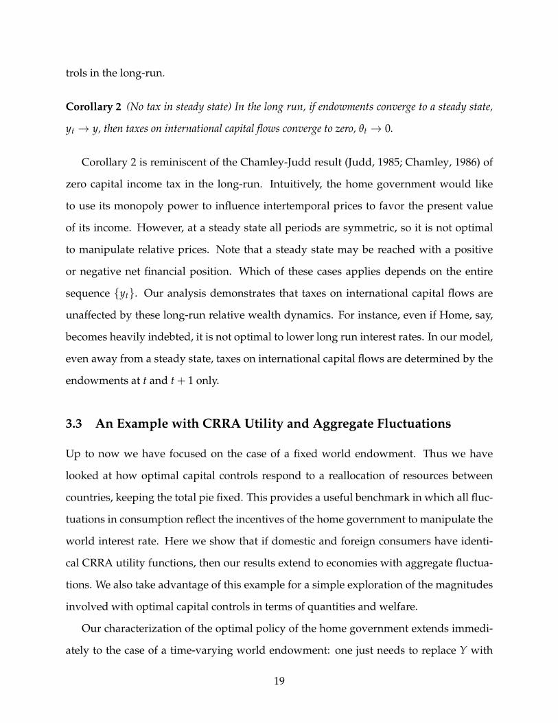
1 Introduction

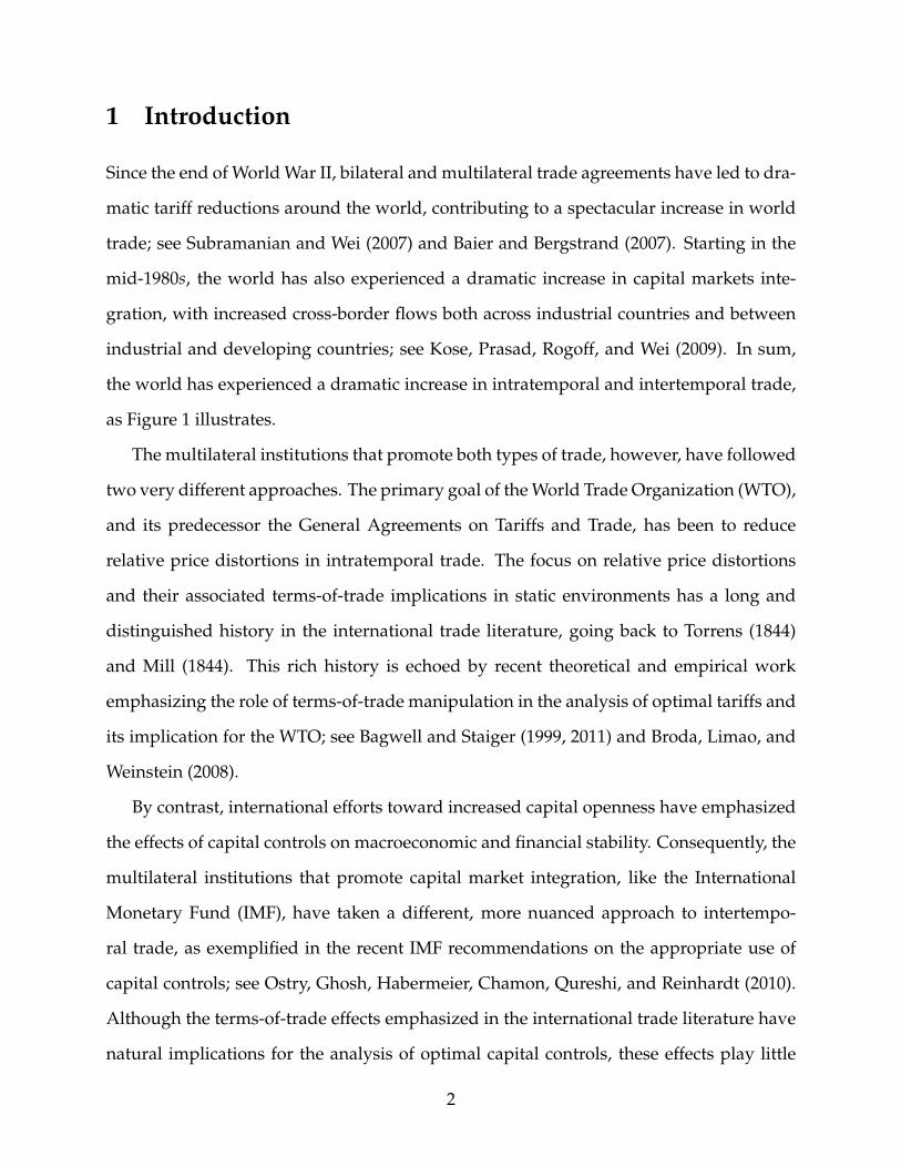
Since the end of World War II, bilateral and multilateral trade agreements have led to dra-

matic tariff reductions around the world, contributing to a spectacular increase in world

trade; see Subramanian and Wei (2007) and Baier and Bergstrand (2007). Starting in the

mid-1980s, the world has also experienced a dramatic increase in capital markets inte-

gration, with increased cross-border flows both across industrial countries and between

industrial and developing countries; see Kose, Prasad, Rogoff, and Wei (2009). In sum,

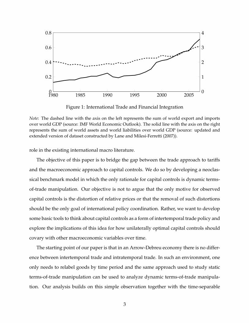
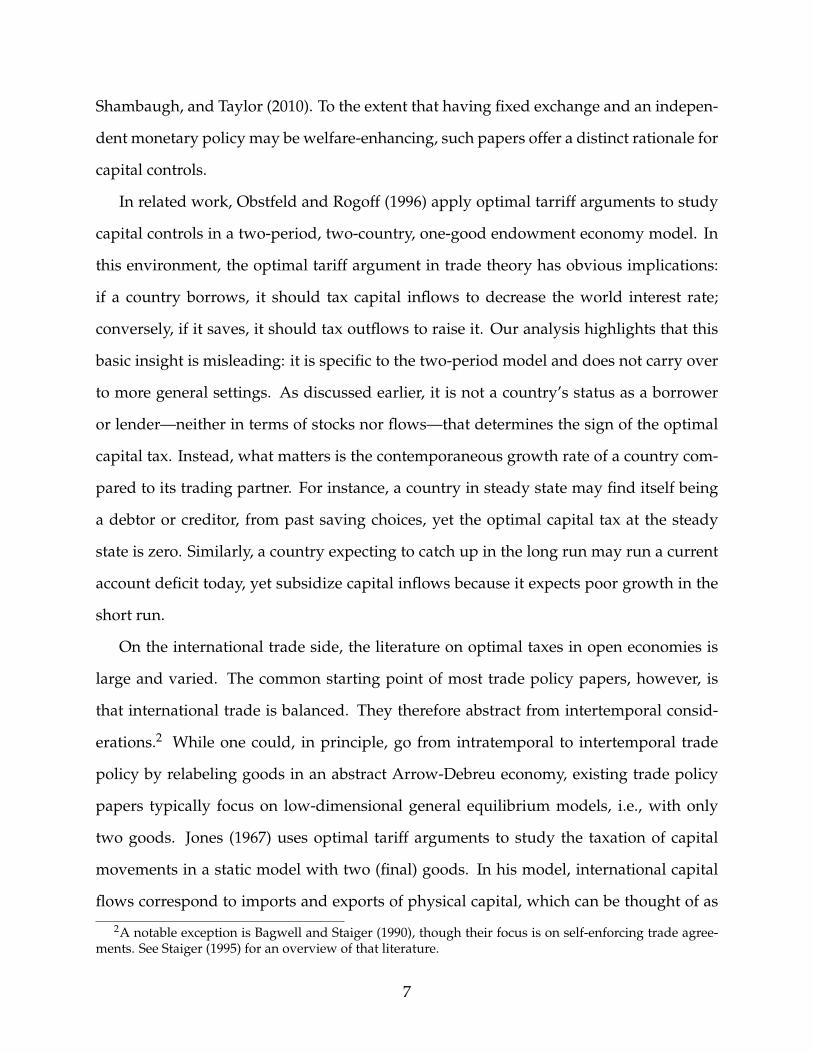
the world has experienced a dramatic increase in intratemporal and intertemporal trade,

as Figure 1 illustrates.

The multilateral institutions that promote both types of trade, however, have followed

two very different approaches. The primary goal of the World Trade Organization (WTO),

and its predecessor the General Agreements on Tariffs and Trade, has been to reduce

relative price distortions in intratemporal trade. The focus on relative price distortions

and their associated terms-of-trade implications in static environments has a long and

distinguished history in the international trade literature, going back to Torrens (1844)

and Mill (1844). This rich history is echoed by recent theoretical and empirical work

emphasizing the role of terms-of-trade manipulation in the analysis of optimal tariffs and

its implication for the WTO; see Bagwell and Staiger (1999, 2011) and Broda, Limao, and

Weinstein (2008).

By contrast, international efforts toward increased capital openness have emphasized

the effects of capital controls on macroeconomic and financial stability. Consequently, the

multilateral institutions that promote capital market integration, like the International

Monetary Fund (IMF), have taken a different, more nuanced approach to intertempo-

ral trade, as exemplified in the recent IMF recommendations on the appropriate use of

capital controls; see Ostry, Ghosh, Habermeier, Chamon, Qureshi, and Reinhardt (2010).

Although the terms-of-trade effects emphasized in the international trade literature have

natural implications for the analysis of optimal capital controls, these effects play little

2

1980 1985 1990 1995 2000 20050

0.2

0.4

0.6

0.8

0

1

2

3

4

Figure 1: International Trade and Financial Integration

Note: The dashed line with the axis on the left represents the sum of world export and importsover world GDP (source: IMF World Economic Outlook). The solid line with the axis on the rightrepresents the sum of world assets and world liabilities over world GDP (source: updated andextended version of dataset constructed by Lane and Milesi-Ferretti (2007)).

role in the existing international macro literature.

The objective of this paper is to bridge the gap between the trade approach to tariffs

and the macroeconomic approach to capital controls. We do so by developing a neoclas-

sical benchmark model in which the only rationale for capital controls is dynamic terms-

of-trade manipulation. Our objective is not to argue that the only motive for observed

capital controls is the distortion of relative prices or that the removal of such distortions

should be the only goal of international policy coordination. Rather, we want to develop

some basic tools to think about capital controls as a form of intertemporal trade policy and

explore the implications of this idea for how unilaterally optimal capital controls should

covary with other macroeconomic variables over time.

The starting point of our paper is that in an Arrow-Debreu economy there is no differ-

ence between intertemporal trade and intratemporal trade. In such an environment, one

only needs to relabel goods by time period and the same approach used to study static

terms-of-trade manipulation can be used to analyze dynamic terms-of-trade manipula-

tion. Our analysis builds on this simple observation together with the time-separable

3

structure of preferences typically used in macro applications.

One key insight that emerges from our analysis is that for a country trading intertem-

porally, unilaterally optimal capital controls are not guided by the absolute desire to alter

the intertemporal price of goods produced in a given period, but rather by the relative

strength of this desire between two consecutive periods. If a country is a net seller of

goods dated t and t + 1 in equal amounts, and faces equal elasticities in both periods,

there is no incentive for the country to distort the saving decisions of its consumers at

date t. It is the time variation in the incentive to distort intertemporal prices that leads to

non-zero capital controls. This is a general principle that, to our knowledge, is novel both

to the international macro and international trade literature.

To illustrate this general principle in the simplest possible way, we first consider an

infinite horizon, two-country, one-good endowment economy. In this model the only rel-

ative prices are real interest rates. We solve for the unilaterally optimal taxes on interna-

tional capital flows in one country, Home, under the assumption that the other country,

Foreign, is passive.1 In this environment, the principle described above has sharp im-

plications for the direction of optimal capital flow taxes. In particular, it is optimal for

Home to tax capital inflows (or subsidize capital outflows) in periods in which Home is

growing faster than the rest of the world and to tax capital outflows (or subsidize capital

inflows) in periods in which it is growing more slowly. Accordingly, if relative endow-

ments converge to a steady state, then taxes on international capital flows converge to

zero. Although our theory of capital controls emphasizes interest rate manipulation, the

sign of taxes on capital flows only depends on the growth rate of the economy relative to

the rest of the world. Home may be a net saver or a net borrower; Home may have a pos-

itive or a negative net financial position; if Home grows faster than the rest of the world,

1Throughout our analysis, we assume that the home government can freely commit at date 0 to a se-quence of taxes. In the economic environment considered in this paper, this is a fairly mild assumption.As we formally establish in Section 3.4, if the home government can enter debt commitments at all maturi-ties, as in Lucas and Stokey (1983), the optimal sequence of taxes under commitment is time-consistent. Tothe extent that bonds of different maturities are available in practice—and they are—we therefore view themodel with commitment as the most natural benchmark for the question that we are interested in.

4

it has incentives to promote domestic savings by taxing capital inflows or subsidizing

capital outflows.

The intuition for our results is as follows. Consider Home’s incentives to distort do-

mestic consumption in each period. In periods of larger trade deficits, it has a stronger

incentive, as a buyer, to distort prices downward by lowering domestic consumption.

Similarly, in periods of larger trade surpluses, it has a stronger incentive, as a seller, to

distort prices upward by raising domestic consumption. Since periods of faster growth

at home tend to be associated with either lower future trade deficits or larger future trade

surpluses, Home always has an incentive to raise future consumption relative to current

consumption in such periods. This is exactly what taxes on capital inflows or subsidies on

capital outflows accomplish through their effects on relative distortions across periods.

The second part of our paper explores further the frontier between international macro

and international trade policy by introducing multiple goods, thereby allowing for both

intertemporal and intratemporal trade. In order to maintain the focus of our analysis

on capital controls, we assume that Home can still choose its taxes on capital flows uni-

laterally, but that it is constrained by a free-trade agreement that prohibits good-specific

taxes/subsidies in all periods. In this environment, we show that the incentive to dis-

tort trade over time does not depend only on the overall growth of the country’s output

relative to the world, but also on its composition.

We illustrate the role of these compositional effects in two ways. First, we establish a

general formula that relates intertemporal distortions to the covariance between the price

elasticities of different goods and the change in the value of home endowments. Ceteris

paribus, we show that Home is more likely to raise aggregate consumption if a change in

the value of home endowments is tilted towards goods whose prices are more manipula-

ble. In this richer environment, even a country that is too small to affect world interest rate

may find it optimal to impose capital controls for terms-of-trade considerations as long

as it is large enough to affect some intratemporal prices. Second, we illustrate through a

5

simple analytical example how such compositional issues relate to cross-country differ-

ences in demand. In a multi good world in which countries have different preferences,

a change in the time profile of consumption not only affects the interest rate but also the

relative prices of consumption goods in each given period. This is an effect familiar from

the literature on the transfer problem, which goes back to the debate between Keynes

(1929) and Ohlin (1929). In our context this means that by distorting its consumers’ deci-

sion to allocate spending between different periods a country also affects its static terms

of trade. Even if all static trade distortions are banned by a free-trade agreement, our

analysis demonstrates that, away from steady state, intratemporal prices may not be at

their undistorted levels if capital controls are allowed.

We conclude by returning to the issue of capital controls and international coopera-

tion, or lack thereof, alluded to at the beginning of our introduction. We consider the case

of capital control wars in which the two countries simultaneously set taxes on capital

flows optimally at date 0, taking as given the sequence of taxes chosen by the other coun-

try. Using a simple quantitative example, we show that far from canceling each other out,

capital controls imposed by both countries aggravate the misallocation of international

capital flows.

Our paper attacks an international macroeconomic question following a classical ap-

proach from the international trade literature and using tools from the dynamic pub-

lic finance literature. In international macro, there is a growing theoretical literature

demonstrating, among other things, how restrictions on international capital flows may

be welfare-enhancing in the presence of various credit market imperfections; see e.g.

Calvo and Mendoza (2000), Caballero and Lorenzoni (2007), Aoki, Benigno, and Kiyotaki

(2010), Jeanne and Korinek (2010), and Martin and Taddei (2010). In addition to these

second-best arguments, there also exists an older literature emphasizing the so-called

“trilemma”: one cannot have a fixed exchange rate, an independent monetary policy and

free capital mobility; see e.g. McKinnon and Oates (1966), or more recently, Obstfeld,

6

Shambaugh, and Taylor (2010). To the extent that having fixed exchange and an indepen-

dent monetary policy may be welfare-enhancing, such papers offer a distinct rationale for

capital controls.

In related work, Obstfeld and Rogoff (1996) apply optimal tarriff arguments to study

capital controls in a two-period, two-country, one-good endowment economy model. In

this environment, the optimal tariff argument in trade theory has obvious implications:

if a country borrows, it should tax capital inflows to decrease the world interest rate;

conversely, if it saves, it should tax outflows to raise it. Our analysis highlights that this

basic insight is misleading: it is specific to the two-period model and does not carry over

to more general settings. As discussed earlier, it is not a country’s status as a borrower

or lender—neither in terms of stocks nor flows—that determines the sign of the optimal

capital tax. Instead, what matters is the contemporaneous growth rate of a country com-

pared to its trading partner. For instance, a country in steady state may find itself being

a debtor or creditor, from past saving choices, yet the optimal capital tax at the steady

state is zero. Similarly, a country expecting to catch up in the long run may run a current

account deficit today, yet subsidize capital inflows because it expects poor growth in the

short run.

On the international trade side, the literature on optimal taxes in open economies is

large and varied. The common starting point of most trade policy papers, however, is

that international trade is balanced. They therefore abstract from intertemporal consid-

erations.2 While one could, in principle, go from intratemporal to intertemporal trade

policy by relabeling goods in an abstract Arrow-Debreu economy, existing trade policy

papers typically focus on low-dimensional general equilibrium models, i.e., with only

two goods. Jones (1967) uses optimal tariff arguments to study the taxation of capital

movements in a static model with two (final) goods. In his model, international capital

flows correspond to imports and exports of physical capital, which can be thought of as

2A notable exception is Bagwell and Staiger (1990), though their focus is on self-enforcing trade agree-ments. See Staiger (1995) for an overview of that literature.

7

a third (intermediate) good. Compared to the present analysis, there is no intertemporal

borrowing and lending. Other exceptions featuring more than two goods only offer: (i)

partial equilibrium results under the assumption of quasi-linear preferences; (ii) suffi-

cient conditions under which seemingly paradoxical results may arise, see e.g. Feenstra

(1986) and Itoh and Kiyono (1987); or (iii) fairly weak restriction on the structure of op-

timal trade policy, see e.g. Dixit (1985) and Bond (1990). To summarize there are no

‘off-the-shelf’ results from the existing trade literature that directly apply to the dynamic

environment considered in our paper.

In terms of methodology, we follow the dynamic public finance literature and use the

primal approach to characterize first optimal wedges rather than explicit policy instru-

ments; see e.g. Lucas and Stokey (1983). Since there are typically many ways to imple-

ment the optimal allocation in an intertemporal context, this approach will help us clarify

the equivalence between capital controls and other policy instruments. Our focus on the

optimal structure of taxes in an open economy is also related to Anderson (1991) and An-

derson and Young (1992). Compared to the present paper, both papers focus on the case

of a small-open economy in which the rationale for taxes is the financing of an exogenous

stream of government expenditures rather than the manipulation of intertemporal and

intratemporal terms-of-trade. Finally, since our theory of capital controls models one of

the two governments as a dynamic monopolist optimally choosing the pattern of con-

sumption over time, our analysis bears some resemblance to the problem of a dynamic

monopolist optimally choosing the rate of extraction of some exhaustible resources; see

Stiglitz (1976).

The rest of our paper is organized as follows. Section 2 describes a simple one-good

economy. Section 3 characterizes the structure of optimal capital controls in this envi-

ronment. Section 4 extends our results to the case of arbitrarily many goods. Section 5

considers the case of capital control wars. Section 6 offers some concluding remarks.

8

2 Basic Environment

2.1 A Dynamic Endowment Economy

There are two countries, Home and Foreign. Time is discrete and infinite, t = 0, 1, ...

and there is no uncertainty. The preferences of the representative consumer at home are

represented by the additively separable utility function:

∞

∑t=0

βtu(ct),

where ct denotes consumption; u is a twice continuously differentiable, strictly increasing,

and strictly concave function, with limc→0 u′(c) = ∞; and β ∈ (0, 1) is the discount factor.

The preferences of the representative consumer abroad have a similar form, with asterisks

denoting foreign variables.

Both domestic and foreign consumers receive an endowment sequence denoted by

{yt} and {y∗t }, respectively. Endowments are bounded away from zero in all periods

in both countries. We make two simplifying assumptions: world endowments are fixed

across periods, yt + y∗t = Y, and the home and foreign consumer have the same discount

factor, β = β∗. Accordingly, in the absence of distortions, there should be perfect con-

sumption smoothing across time in both countries.3

We assume that both countries begin with zero assets at date 0.4 Let pt be the price of

a unit of consumption in period t on the world capital markets. In the absence of taxes,

the intertemporal budget constraint of the home consumer is

∞

∑t=0

pt(ct − yt) ≤ 0.

The budget constraint of of the foreign consumer is the same expression with asterisks on

3In Section 3.3 we demonstrate that our results generalize to environment with aggregate fluctuations ifconsumers have Constant Relative Risk Aversion (CRRA) utility.

4The assumption of zero initial assets is relaxed in Section 3.4.

9

ct and yt.

2.2 A Dynamic Monopolist

For most of the paper, we will focus on the case in which the home government sets taxes

on capital flows in order to maximize domestic welfare, assuming the foreign government

is passive: it does not have any tax policy in place and does not respond to variations in

the home policy. We will look at the case where both governments set taxes strategically

in Section 5.

In order to characterize the optimal policy of the home government, we follow the

dynamic public finance literature and use the primal approach. That is, we approach

the optimal policy problem of the home government by studying a planning problem in

which equilibrium quantities are chosen directly and address implementation issues later.

Formally, we assume that the objective of the home government is to maximize the

lifetime utility of the representative domestic consumer subject to (i) utility maximization

by the foreign consumer at (undistorted) world prices pt, and (ii) market clearing in each

period. The foreign consumer first-order conditions are given by

βtu∗′(c∗t ) = λ∗pt, (1)∞

∑t=0

pt(c∗t − y∗t ) = 0, (2)

where λ∗ is the Lagrange multiplier on the foreign consumer’s budget constraint. More-

over, goods market clearing requires

ct + c∗t = Y. (3)

Combining equations (1)-(3), we can express the planning problem of the home govern-

10

ment as

max{ct}

∞

∑t=0

βtu(ct) (P)

subject to∞

∑t=0

βtu∗′(Y− ct)(ct − yt) = 0. (4)

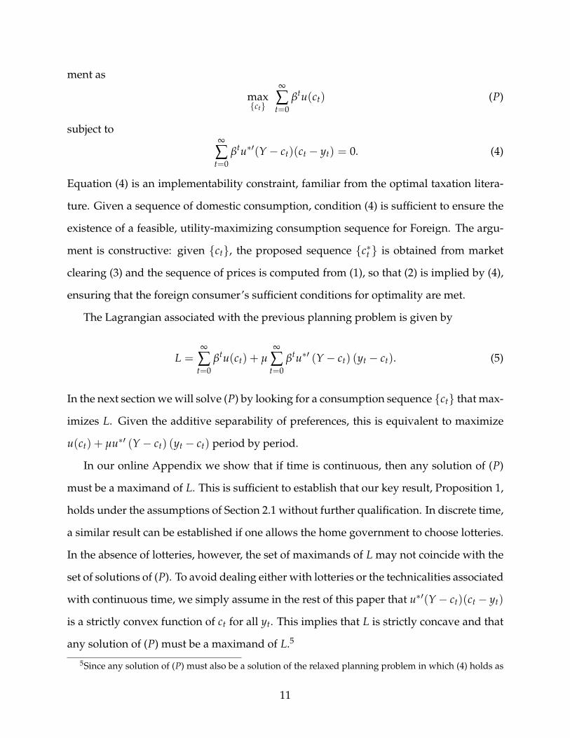
Equation (4) is an implementability constraint, familiar from the optimal taxation litera-

ture. Given a sequence of domestic consumption, condition (4) is sufficient to ensure the

existence of a feasible, utility-maximizing consumption sequence for Foreign. The argu-

ment is constructive: given {ct}, the proposed sequence {c∗t } is obtained from market

clearing (3) and the sequence of prices is computed from (1), so that (2) is implied by (4),

ensuring that the foreign consumer’s sufficient conditions for optimality are met.

The Lagrangian associated with the previous planning problem is given by

L =∞

∑t=0

βtu(ct) + µ∞

∑t=0

βtu∗′ (Y− ct) (yt − ct). (5)

In the next section we will solve (P) by looking for a consumption sequence {ct} that max-

imizes L. Given the additive separability of preferences, this is equivalent to maximize

u(ct) + µu∗′ (Y− ct) (yt − ct) period by period.

In our online Appendix we show that if time is continuous, then any solution of (P)

must be a maximand of L. This is sufficient to establish that our key result, Proposition 1,

holds under the assumptions of Section 2.1 without further qualification. In discrete time,

a similar result can be established if one allows the home government to choose lotteries.

In the absence of lotteries, however, the set of maximands of L may not coincide with the

set of solutions of (P). To avoid dealing either with lotteries or the technicalities associated

with continuous time, we simply assume in the rest of this paper that u∗′(Y− ct)(ct − yt)

is a strictly convex function of ct for all yt. This implies that L is strictly concave and that

any solution of (P) must be a maximand of L.5

5Since any solution of (P) must also be a solution of the relaxed planning problem in which (4) holds as

11

3 Optimal Capital Controls

3.1 Optimal Allocation

We first describe how home consumption {ct} fluctuates with home endowments {yt}along the optimal path. Next we will show how the optimal allocation can be imple-

mented using taxes on international capital flows.

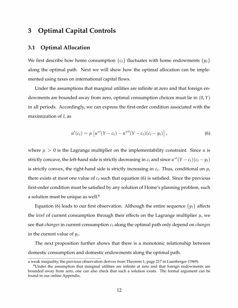
Under the assumptions that marginal utilities are infinite at zero and that foreign en-

dowments are bounded away from zero, optimal consumption choices must lie in (0, Y)

in all periods. Accordingly, we can express the first-order condition associated with the

maximization of L as

u′(ct) = µ[u∗′(Y− ct)− u∗′′(Y− ct)(ct − yt)

], (6)

where µ > 0 is the Lagrange multiplier on the implementability constraint. Since u is

strictly concave, the left-hand side is strictly decreasing in ct and since u∗′(Y− ct)(ct− yt)

is strictly convex, the right-hand side is strictly increasing in ct. Thus, conditional on µ,

there exists at most one value of ct such that equation (6) is satisfied. Since the previous

first-order condition must be satisfied by any solution of Home’s planning problem, such

a solution must be unique as well.6

Equation (6) leads to our first observation. Although the entire sequence {yt} affects

the level of current consumption through their effects on the Lagrange multiplier µ, we

see that changes in current consumption ct along the optimal path only depend on changes

in the current value of yt.

The next proposition further shows that there is a monotonic relationship between

domestic consumption and domestic endowments along the optimal path.

a weak inequality, the previous observation derives from Theorem 1, page 217 in Luenberger (1969).6Under the assumption that marginal utilities are infinite at zero and that foreign endowments are

bounded away from zero, one can also check that such a solution exists. The formal argument can befound in our online Appendix.

12

0 ct yt cs ys Y

u′(c)

µ[u∗′(Y− c) + u∗′′(Y− c)(yt − c)]

µu∗′(Y− c)

µ[u∗′(Y− c) + u∗′′(Y− c)(ys − c)]

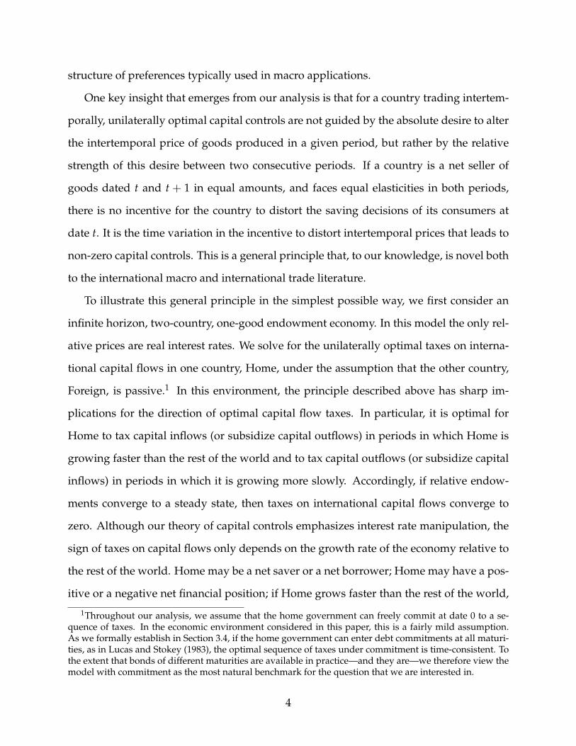
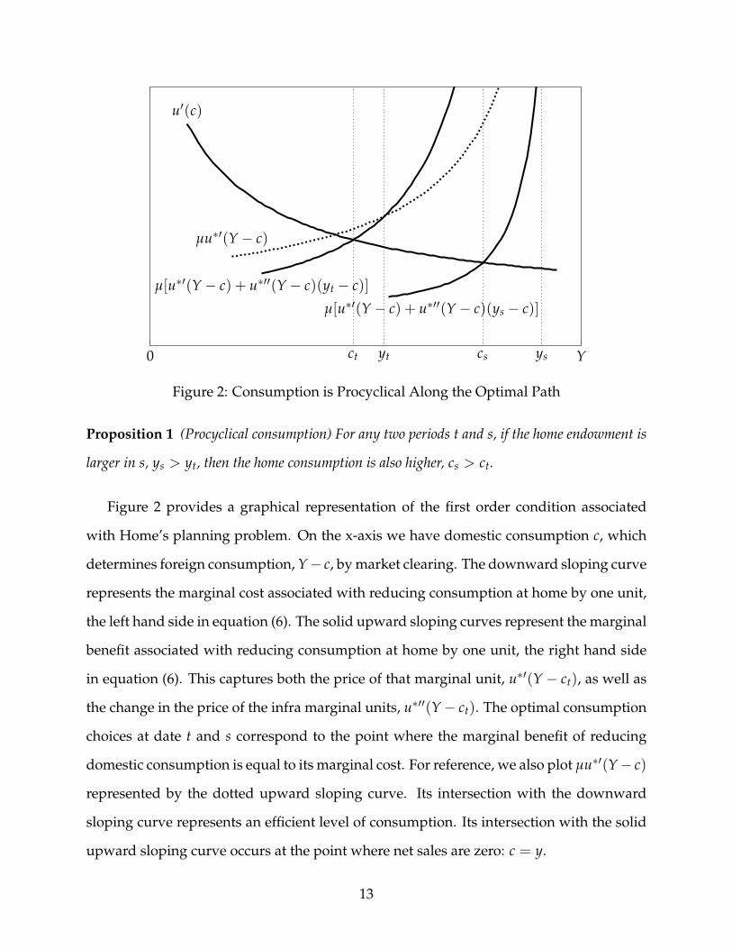
Figure 2: Consumption is Procyclical Along the Optimal Path

Proposition 1 (Procyclical consumption) For any two periods t and s, if the home endowment is

larger in s, ys > yt, then the home consumption is also higher, cs > ct.

Figure 2 provides a graphical representation of the first order condition associated

with Home’s planning problem. On the x-axis we have domestic consumption c, which

determines foreign consumption, Y− c, by market clearing. The downward sloping curve

represents the marginal cost associated with reducing consumption at home by one unit,

the left hand side in equation (6). The solid upward sloping curves represent the marginal

benefit associated with reducing consumption at home by one unit, the right hand side

in equation (6). This captures both the price of that marginal unit, u∗′(Y − ct), as well as

the change in the price of the infra marginal units, u∗′′(Y− ct). The optimal consumption

choices at date t and s correspond to the point where the marginal benefit of reducing

domestic consumption is equal to its marginal cost. For reference, we also plot µu∗′(Y− c)

represented by the dotted upward sloping curve. Its intersection with the downward

sloping curve represents an efficient level of consumption. Its intersection with the solid

upward sloping curve occurs at the point where net sales are zero: c = y.

13

Figure 2 gives the intuition for Proposition 1. As the endowment increases from yt

to ys, the curve u′(c) does not move. At the same time, the marginal benefit curve shifts

down, as the price decrease associated to a reduction in c applies to a larger amount

of inframarginal units sold. This induces Home to consume more, explaining why con-

sumption is procyclical along the optimal path.7

As a preliminary step in the analysis of optimal capital flow taxes, we conclude this

section by describing how the “wedge” between the marginal utility of domestic and

foreign consumption varies along the optimal path. Formally, define

τt ≡u′(ct)

µu∗′(c∗t )− 1. (7)

By market clearing, we know that c∗t = Y − ct. Thus combining the definition of τt with

the strict concavity of u and u∗, we obtain the following corollary to Proposition 1.

Corollary 1 (Countercyclical wedges) For any two periods t and s, if the home endowment is

larger in s, ys > yt, then the wedge is lower, τs < τt.

At this point, it is worth pausing to discuss how Corollary 1 relates to and differs from

existing results in the trade policy literature. By equations (6) and (7), we have

τt = −u∗′′(Y− ct)

u∗′(Y− ct)(ct − yt). (8)

Condition (8) is closely related to the well-known optimal tariff formula involving the

elasticity of the foreign export supply curve in static trade models with two goods and/or

quasi-linear preferences. This should not be too surprising since τt measures the differ-

7To see why the strict convexity of u∗′(Y − ct)(ct − yt) in ct is not crucial for establishing Proposition 1,note that any sequence {ct} that maximizes L must be such that ct ∈ arg max u(c) + µu∗′ (Y− c) (yt − c)period by period. Under the assumption that u∗ is strictly concave, u(c) + µu∗′ (Y− c) (yt − c) satisfies thesingle-crossing property in (c, yt). Thus the set of consumption levels that maximize L must be increasingin yt in the strong set order. To establish that consumption is procyclical along the optimal path, the onlytechnical question then is whether any solution of (P) can be recovered as a maximand of L for some valueof µ. As we already discussed at the end of Section 2.2, the answer in continuous time is always yes.

14

ence between the marginal utility of domestic and foreign consumption. According to

equation (8), the wedge τt is positive in periods of trade deficit and negative in periods

of trade surplus. This captures the idea that if (time-varying) trade taxes were available,

Home would like to tax imports if ct − yt > 0 and tax exports if ct − yt < 0. Corollary 1,

however, goes beyond this simple observation by establishing a monotonic relationship

between τt and yt. This novel insight will play a key role in our analysis of optimal capital

controls.

3.2 Optimal Taxes on International Capital Flows

It is well-known from the Ramsey taxation literature that there are typically many com-

binations of taxes that can implement the optimal allocation; see e.g. Chari and Kehoe

(1999). Here, we focus on the tax instrument most directly related to world interest rate

manipulation: taxes on international capital flows.8

For expositional purposes, we assume that consumers can only trade one-period bonds

on international capital markets, with the home government imposing a proportional tax

θt on the gross return on net asset position in international bond markets. Standard ar-

guments show that any competitive equilibrium supported by intertemporal trading of

consumption claims at date 0 can be supported by trading of one-period bonds. As we

discuss later in Section 3.4, none of the results presented here depend on the assumption

that one-period bonds are the only assets available.

With only one-period bonds, the per-period budget constraint of the home consumer

takes the form

qtat+1 + ct = yt + (1− θt−1) at − lt, (9)

where at denotes the current bond holdings, lt is a lump sum tax, and qt ≡ pt+1/pt is

8Other tax instruments that could be used to implement the optimal allocation include time-varyingtrade and consumption taxes (possibly accompanied by production taxes in more general environments).See Jeanne (2011) for a detailed discussion of the equivalence between capital controls and trade taxes.

15

the price of one-period bonds at date t. In addition, consumers are subject to a standard

no-Ponzi condition, limt→∞ ptat ≥ 0. In this environment the home consumer’s Euler

equation takes the form

u′(ct) = β(1− θt)(1 + rt)u′(ct+1). (10)

where rt ≡ 1/qt − 1 is the world interest rate. Given a solution {ct} to Home’s planning

problem (P), the world interest rate is uniquely determined as

rt =u∗′(Y− ct)

βu∗′(Y− ct+1)− 1, (11)

by equations (1) and (3). Thus, given {ct}, we can use (10) to construct a unique sequence

of taxes {θt}. We can then set the sequence of assets positions and lump-sum transfers

at =∞

∑s=t

(ps/pt) (cs − ys) ,

lt = −θt−1at,

which ensures that the per-period budget constraint (9) and the no-Ponzi condition are

satisfied. Since (9), (10), and the no-Ponzi condition are sufficient for optimality it follows

that given prices and taxes, {ct} is optimal for the home consumer. This establishes that

any solution {ct} of (P) can be decentralized as a competitive equilibrium with taxes.

A positive θt can be interpreted as imposing simultaneously a tax θt on capital out-

flows and a subsidy θt to capital inflows. Obviously, since there is a representative con-

sumer, only one of the two is active in equilibrium: the outflow tax if the country is a net

lender, at+1 > 0, and the inflow subsidy if it is a net borrower, at+1 < 0. Similarly, a neg-

ative θt can be interpreted as a subsidy on capital outflows plus a tax on capital inflows.

The bottom line is that θt > 0 discourages domestic savings while θt < 0 encourages

them.

16

Combining the definition of the wedge (7) with equations (10) and (11), we obtain the

following relationship between wedges and taxes on capital flows:

θt = 1− 1 + τt

1 + τt+1. (12)

The previous subsection has already established that variations in domestic consumption

ct along the optimal path are only a function of the current endowment yt. Since τt is

only a function of ct, equation (12) implies that variations in θt are only a function of yt

and yt+1. Combining equation (12) with Corollary 1, we then obtain the following result

about the structure of optimal capital controls.

Proposition 2 (Optimal capital flow taxes) Suppose that the optimal policy is implemented with

capital flows taxes. Then it is optimal:

1. to tax capital inflows/subsidize capital outflows (θt < 0) if yt+1 > yt;

2. to tax capital outflows/subsidize capital inflows (θt > 0) if yt+1 < yt;

3. not to distort capital flows (θt = 0) if yt+1 = yt.

Proposition 2 builds on the same logic as Proposition 1. Suppose, for instance, that

Home is running a trade deficit in periods t and t + 1. In this case, the home govern-

ment wants to exercise its monopsony power by lowering domestic consumption in both

periods. But if Home grows between these two periods, yt+1 > yt, the number of units

imported from abroad is lower in period t + 1. Thus the home government has less in-

centive to lower consumption in that period. This explains why a tax on capital inflows is

optimal in period t: it reduces borrowing in period t, thereby shifting consumption from

period t to period t + 1. The other results follow a similar logic.

It is worth emphasizing that, although the only motive for capital controls in our

model is interest rate manipulation, neither the net financial position of Home nor the

17

change in that position are the relevant variables to look at to sign the optimal direction

of the tax in any particular period. This is because the effect of a capital flow tax is to

affect the relative distortion in consumption decisions between two consecutive periods.

Therefore, what matters is whether the monopolistic/monopsonistic incentives to restrict

domestic consumption are stronger in period t or t + 1. In our simple endowment econ-

omy, these incentives are purely captured by the growth rate of the endowment, but the

same broad principle would extend to more general environments.

Proposition 2 has a number of implications. Consider first an economy that is catching

up with the rest of the world in the sense that yt+1 > yt for all t. According to our analysis,

it is optimal for this country to tax capital inflows and to subsidize capital outflows. The

basic intuition is that a growing country will export more tomorrow than today. Thus it

has more incentive to increase export prices in the future, which it can achieve by raising

future consumption through a subsidy on capital outflows. For an economy catching up

with the rest of the world, larger benefits from future terms-of-trade manipulation are

associated with taxes and subsidies that encourage domestic savings.

Consider instead a country that at time t borrows from abroad in anticipation of a

temporary boom. In particular, suppose that yt+1 > yt and ys = yt for all s > t + 1. In

this situation, the logic of Proposition 2 implies that, at time t, at the onset of the boom, it

is optimal to impose restrictions on short-term capital inflows, i.e., to tax bonds with one-

period maturity and leave long-term capital inflows unrestricted.9 This example provides

a different perspective on why governments may try to alter the composition of capital

flows in favor of longer maturity flows in practice; see Magud, Reinhart, and Rogoff

(2011). In our model, incentives to alter the composition of capital flows do not come

from the fear of “hot money” but from larger benefits of terms-of-trade manipulation in

the short run.

Finally, Proposition 2 has sharp implications for the structure of optimal capital con-

9The tax on two period bonds is easily shown to be (1− θt)(1− θt+1)− 1 and Proposition 1 implies thatit is zero in our example.

18

trols in the long-run.

Corollary 2 (No tax in steady state) In the long run, if endowments converge to a steady state,

yt → y, then taxes on international capital flows converge to zero, θt → 0.

Corollary 2 is reminiscent of the Chamley-Judd result (Judd, 1985; Chamley, 1986) of

zero capital income tax in the long-run. Intuitively, the home government would like

to use its monopoly power to influence intertemporal prices to favor the present value

of its income. However, at a steady state all periods are symmetric, so it is not optimal

to manipulate relative prices. Note that a steady state may be reached with a positive

or negative net financial position. Which of these cases applies depends on the entire

sequence {yt}. Our analysis demonstrates that taxes on international capital flows are

unaffected by these long-run relative wealth dynamics. For instance, even if Home, say,

becomes heavily indebted, it is not optimal to lower long run interest rates. In our model,

even away from a steady state, taxes on international capital flows are determined by the

endowments at t and t + 1 only.

3.3 An Example with CRRA Utility and Aggregate Fluctuations

Up to now we have focused on the case of a fixed world endowment. Thus we have

looked at how optimal capital controls respond to a reallocation of resources between

countries, keeping the total pie fixed. This provides a useful benchmark in which all fluc-

tuations in consumption reflect the incentives of the home government to manipulate the

world interest rate. Here we show that if domestic and foreign consumers have identi-

cal CRRA utility functions, then our results extend to economies with aggregate fluctua-

tions. We also take advantage of this example for a simple exploration of the magnitudes

involved with optimal capital controls in terms of quantities and welfare.

Our characterization of the optimal policy of the home government extends immedi-

ately to the case of a time-varying world endowment: one just needs to replace Y with

19

Yt in equation (6). Under the assumption of identical CRRA utility functions, u(c) =

u∗(c) = c1−γ/ (1− γ) with γ ≥ 0, this leads to a simple relationship between the home

share of world endowments, yt/Yt, and the home share of world consumption, ct/Yt:

(ct/Yt

1− ct/Yt

)−γ

= µ

[1 + γ

(ct/Yt − yt/Yt

1− ct/Yt

)].

The left-hand side is decreasing in ct/Yt, whereas the right-hand side is increasing in

ct/Yt and decreasing in yt/Yt. Thus the implicit function theorem implies that, along

the optimal path, the home share of world consumption, c/Y, is strictly increasing in

the home share of world endowments, y/Y. Put simply, if utility functions are CRRA,

Proposition 1 generalizes to environments with aggregate fluctuations.

Now consider the wedge τt between the marginal utility of domestic and foreign con-

sumption in period t. Under the assumption of CRRA utility functions we have

τt =1µ

(ct/Yt

1− ct/Yt

)−γ

− 1.

According to this expression, if c/Y is strictly increasing in y/Y along the optimal path,

then τ is strictly decreasing. The same logic as in Section 3.2 therefore implies that optimal

taxes on capital flows must be such that θt < 0 if and only if yt+1/Yt+1 > yt/Yt. In other

words, if utility functions are CRRA, Proposition 2 also generalizes to environments with

aggregate fluctuations.

As a quantitative illustration of our theory of capital controls as dynamic terms-of-

trade manipulation, suppose that foreign endowments {y∗t } are growing at the constant

rate g = 3% per year and that Home is catching up with the rest of the world. To be more

specific, suppose that the home endowment is 1/6 of world endowments at date 0 and

that it is converging towards being 1/3 in the long run, with the ratio yt/y∗t converging

20

0 20 40 60-0.01

-0.008

-0.006

-0.004

-0.002

0

θ

capital flows tax and net assets

0 20 40 600.15

0.2

0.25

0.3

0.35y/

Y,c

/Y

output and consumption

-3

-1.5

0

a/Y

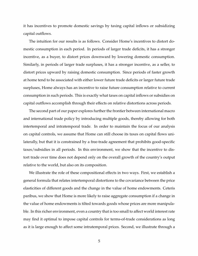
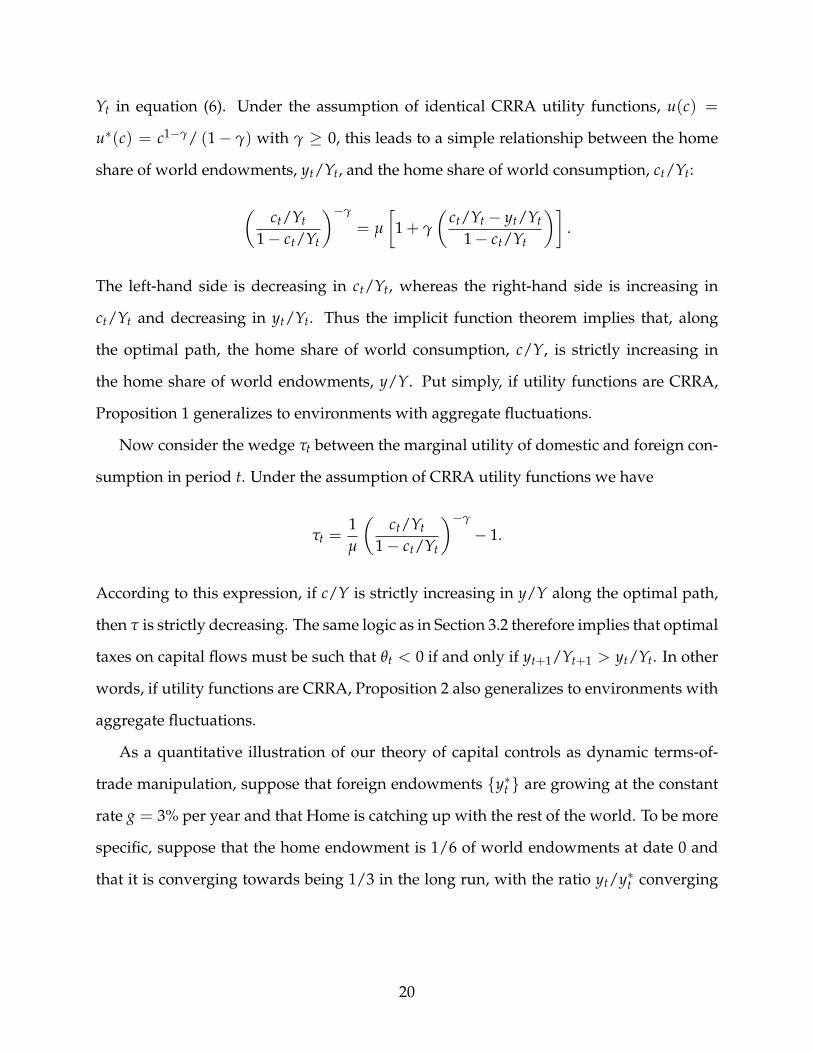
Figure 3: Optimal Allocation and Taxes in a Country Catching Up

Note: In the left panel, the steeper solid line is the exogenous path for the endowment, the flatterdashed line is consumption at the optimal policy of the home government, and the dotted lineis the efficient no-tax benchmark. In the right panel, the upward sloping solid line with axis onthe left is the capital flow tax and the downward sloping dashed line with axis on the right is thehome assets-to-world-GDP ratio.

to its long run value at a constant speed η = 0.05.10

Figure 3 shows the path of the home share of world endowments and consumption,

assuming a unit elasticity of intertemporal substitution, γ = 1. For comparison, we also

plot the path for consumption in the benchmark case with no capital controls. In this

case, consistently with consumption smoothing, Home consumes a fixed fraction of the

world endowment in all periods. Although optimal capital controls reduce consumption

smoothing, intertemporal trade flows are several times larger than domestic output. The

optimal tax on capital inflows is less than 1% at date 0 and vanishing in the long run,

following the same logic as for Corollary 2. We see that that the optimal tax on capital

inflows decreases as the value of the home debt increases. Compared to the benchmark with

no capital controls, optimal taxes are associated with an increase in domestic consumption

of 0.12% and a decrease in foreign consumption of 0.07%. Though the welfare impact of

optimal capital controls is admittedly not large in this particular example, it is not much

10That is, we assume thatyt/y∗t − a = (y0/y∗0 − a) e−ηt,

with a = 0.5 > y0/y∗0 = 0.2.

21

0 20 40 60-0.02

-0.014

-0.008

-0.002

0.004

0.01

θ

capital flows tax and net assets

0 20 40 60

0.15

0.2

0.25

0.3y/

Y,c

/Youtput and consumption

-3

-1.5

0

a/Y

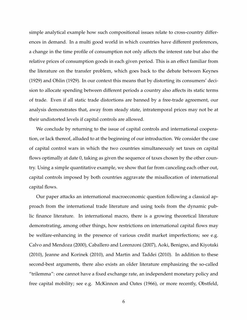
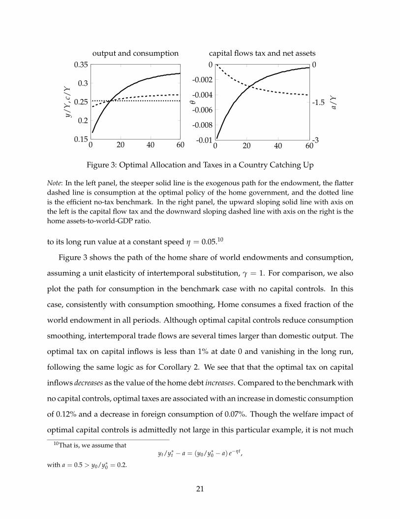
Figure 4: Optimal Allocation and Taxes in a Country Falling Behind Before Catching Up

Note: In the left panel, the steeper solid line is the exogenous path for the endowment, the flatterdashed line is consumption at the optimal policy of the home government, and the dotted lineis the efficient no-tax benchmark. In the right panel, the non-monotonic solid line with axis onthe left is the capital flow tax and the downward sloping dashed line with axis on the right is thehome assets-to-world-GDP ratio.

smaller than either the estimated gains of international trade or financial integration.11

Figure 4 considers an alternative endowment path in which Home falls behind in the

short-run, before catching up in the long-run. As in the previous example, Home is con-

verging towards having 1/3 of world endowments with the ratio yt/y∗t converging to its

long run value at a constant speed η = 0.05. Because of long-run considerations, we see

that Home borrows in all periods. Based on the logic of a two-period model, one might

have therefore expected Home to have incentives to tax capital inflows in all periods to

reduce domestic borrowing, and in turn, the world interest rate. Yet we see that when

falling behind, the home government has incentives to subsidize rather than tax capital in-

flows. As discussed earlier, this occurs because capital controls are guided by the relative

strength of the desire to to alter the intertemporal price of goods between consecutive pe-

riods. In the short-run, the growth rate is negative, hence the subsidy on capital inflows.

11According to a fairly large class of trade models, the welfare gains from international trade in theUnited States are between 0.7% and 1.4% of real GDP; see Arkolakis, Costinot, and Rodriguez-Clare (2012).Similarly, the welfare gains from switching from financial autarky to perfect capital mobility is roughlyequivalent to a 1% permanent increase in consumption for the typical non-OECD country; see Gourinchasand Jeanne (2006).

22

The pattern of borrowing and lending, per se, is irrelevant.12

3.4 Initial Assets, Debt Maturity, and Time-Consistency

So far, we have focused on environments in which: (i) there are no initial assets at date

0 and (ii) one-period bonds are the only assets available. We now briefly discuss how

relaxing both assumptions affects our results. We also show that if more debt instruments

are available, the optimal allocation is time-consistent: a future government free to choose

future consumption, but forced to fulfill previous debt obligations would not want to

deviate from the consumption path chosen by its predecessors.

Let at,s represents holdings at time t of bonds maturing at time s. Suppose the home

consumer enters date 0 with initial asset holdings {a0,t}∞t=0. The asset holdings now enter

the intertemporal budget constraints of the home and foreign consumers. In particular,

the budget constraint of the foreign consumer generalizes to

∞

∑t=0

pt(c∗t − y∗t − a∗0,t) = 0,

where a∗0,t = −a0,t denotes initial asset holdings abroad. The other equilibrium conditions

are unchanged, so Home’s planning problem becomes

max{ct}

∞

∑t=0

βtu(ct) (P0)

12It should be clear that the reason why a country that borrows may choose to subsidize rather thantax capital inflows is distinct from the reason why a country may find subsidies rather than taxes welfareenhancing in a static model with many goods; see e.g. Feenstra (1986), Itoh and Kiyono (1987), or Bond(1990). In the previous papers, the optimality of subsidies rely on complementarities in demand acrossgoods, which our model with additively separable preferences rules out. Here, imported goods alwaysface a positive wedge, i.e., an import tax, whereas exported goods always face a negative wedge, i.e. anexport tax; see equation (8). The reason why a country that borrows may choose to subsidize capital inflowsis because taxes on one period bonds are related to, but distinct from static trade taxes; see equation (12).Specifically, for a country that borrows, a subsidy on one-period bonds, θt > 0, is equivalent to a time-varying import tax, τt+1 > τt > 0; it does not require import subsidies at any point in time.

23

subject to∞

∑t=0

βtu∗′(Y− ct)(ct − yt + a∗0,t) = 0. (13)

Compared to the case without initial assets, the only difference is the new implementabil-

ity constraint (13) that depends on {yt − a∗0,t} rather than {yt}. Accordingly, Proposition

1 and Corollary 1 simply generalize to environments with initial assets {a∗0,t}∞t=0 provided

that they are restated in terms of changes in yt − a∗0,t rather than changes in yt.

Throughout our analysis, we have assumed that the home government can freely com-

mit at date 0 to a consumption path {ct}. Now that we have recognized the role of the

initial asset positions, this assumption may seem uncomfortably restrictive. After all,

along the optimal path, the debt obligations {a∗t,s}∞s=t held at date t will typically be dif-

ferent from the obligations {a∗0,s}∞s=t held at date 0. Accordingly, a government at later

dates may benefit from deviating from the consumption chosen at date 0.

We now demonstrate that this is not the case if the government has access to bonds

of arbitrary maturity. The basic idea builds on the original insight of Lucas and Stokey

(1983). At any date t, the foreign consumer is indifferent between many future asset

holdings {a∗t+1,s}∞s=t+1. Given a consumption sequence {c∗t } that maximizes her utility

subject to her budget constraint, she is indifferent between any bond holdings satisfying

∞

∑s=t+1

ps(c∗s − y∗s − a∗t+1,s) = 0. (14)

As we show in the appendix, this degree of freedom is sufficient to construct sequences

of debt obligations {a∗t,s}∞s=t for all t ≥ 1 such that the solution of

max{cs}

∞

∑s=t

βsu(cs)

subject to∞

∑s=t

βsu∗′(Y− cs)(cs − ys + a∗t,s) = 0 (15)

24

coincides with the solution of (P0) at all dates t ≥ 0. In short, if the home government can

enter debt commitments at all maturities, the optimal allocation derived in Section 3.1 is

time-consistent.

4 Intertemporal and Intratemporal Trade

How do the incentives to tax capital flows change in a world with many goods? In a one-

good economy, the only form of terms-of-trade manipulation achieved by taxing capital

flows is to manipulate the world interest rate. In a world with many goods, distorting the

borrowing and lending decisions of domestic consumers also affects the relative prices

of the different goods traded in each period. In this section, we explore how these new

intratemporal considerations change optimal capital flow distortions.

In order to maintain the focus of our analysis on optimal capital controls, we proceed

under the assumption that Home is constrained by an international free-trade agreement

that prohibits good specific taxes/subsidies in all periods. As in the previous section,

Home is still allowed to impose taxes on capital flows that distort intertemporal decisions.

This means that while Home cannot control the path of consumption of each specific good

i, it can still control the path of aggregate consumption. As we shall see, in general, the

path of aggregate consumption can affect relative prices at any point in time, thus creating

additional room for terms-of-trade manipulation, even for countries that cannot affect the

world interest rate.

4.1 The Monopolist Problem Revisited

The basic environment is the same as in Section 2.1, except that there are n > 1 goods.

Thus domestic consumption and output, ct and yt, are now vectors in Rn+. We assume

25

that the domestic consumer has additively separable preferences represented by

∞

∑t=0

βtU (Ct) ,

where U is increasing and strictly concave, Ct ≡ g (ct) is aggregate domestic consump-

tion at date t, and g is increasing, concave, and homogeneous of degree one. Analogous

definitions apply to U∗ and C∗t ≡ g∗ (c∗t ).

In the absence of taxes, the intertemporal budget constraint of the home consumer is

now given by∞

∑t=0

pt · (ct − yt) ≤ 0,

where pt ∈ Rn+ denotes the intertemporal price vector for period-t goods and · is the inner

product. A similar budget constraint applies in Foreign.

As in Section 2.2, we use the primal approach to characterize the optimal policy of the

home government. In this new environment, the home government’s objective is to set

consumption {ct} in order to maximize the lifetime utility of its representative consumer

subject to (i) utility maximization by the foreign representative consumer at (undistorted)

world prices pt; (ii) market clearing in each period; and (iii) a free trade agreement that

rules out good specific taxes or subsidies.

Constraint (i) can be dealt with as we did in the one-good case. In vector notation,

the first-order conditions associated with utility maximization by the foreign consumer

generalize to

βtU∗′ (C∗t ) g∗c (c∗t ) = λ∗pt, (16)

∞

∑t=0

pt · (c∗t − y∗t ) = 0. (17)

Next, note that if Home cannot impose good specific taxes or subsidies, the relative price

of any two goods i and j in period t, pit/pjt, must be equal in the two countries and equal

26

to the marginal rates of substitution gi (ct) /gj (ct) and g∗i (c∗t ) /g∗j (c

∗t ). Accordingly, the

consumption allocation (ct, c∗t ) in any period t is Pareto efficient and solves

C∗ (Ct) = maxc,c∗{g∗(c∗) subject to c + c∗ = Y and g(c) ≥ Ct} (18)

for some Ct. Therefore, constraints (ii) and (iii), can be captured by letting Home choose

an aggregate consumption level Ct, which identifies a point on the static Pareto frontier.

The consumption vectors at time t are then given by the corresponding solutions to prob-

lem (18), which we denote by c (Ct) and c∗ (Ct).

We can then state Home’s planning problem in the case of many goods as

max{Ct}

∞

∑t=0

βtU(Ct) (P′)

subject to∞

∑t=0

βtρ(Ct) · (c (Ct)− yt) = 0, (19)

where ρ(Ct) ≡ U∗′ (C∗(Ct))∇g∗(c∗ (Ct)). Equation (19) is the counterpart of the imple-

mentability constraint in Section 2.2. In line with our previous analysis, we assume that

ρ(Ct) · (c (Ct)− yt) is a strictly convex function of Ct. This implies the uniqueness of the

solution to (P′).

4.2 Optimal Allocation

With many goods, the first-order condition associated with Home’s planning problem

generalizes to

U′ (Ct) = µ

[ρ(Ct) ·

∂c(Ct)

∂Ct+

∂ρ(Ct)

∂Ct· (c(Ct)− yt)

], (20)

27

where µ still denotes the Lagrange multiplier on the implementability constraint. Armed

with condition (20), we can now follow the same strategy as in the one-good case. First

we will characterize how {Ct} covaries with {yt} along the optimal path. Second we will

derive the associated implications for the structure of optimal capital controls.

The next proposition describes the relationship between domestic consumption and

domestic endowments along the optimal path.

Proposition 3 (Procyclical aggregate consumption) Suppose that between periods t and t + 1

there is a small change in the home endowment dyt+1 = yt+1 − yt. Then the home consumption

is higher in period t + 1, Ct+1 > Ct, if and only if ∂ρ(Ct)/∂Ct · dyt+1 > 0.

In the one good case, ∂ρ(Ct)/∂Ct simplifies to −u∗′′(Y − ct), which is positive by the

concavity of u∗. Therefore, whether domestic consumption grows or not only depends on

whether the level of domestic endowments is increasing or decreasing. In the multi-good

case, by contrast, this also depends on the composition of domestic endowments and on

how relative prices respond to changes in Ct.

In order to highlight the importance of these compositional effects, in an economy

with many goods, consider the effect of a small change in domestic endowment that

leaves its market value unchanged at period t prices. That is, suppose ρ(Ct) · dyt+1 = 0. In

the one good case this can only happen if the endowment level does not change, thereby

leading to a zero capital flow tax. In the multi-good case this is no longer true. According

to Proposition 3, consumption would grow if and only if

Cov(

ρ′i(Ct)

ρi(Ct), ρi(Ct)dyit+1

)> 0.

Here, what matters is whether the composition of endowments tilts towards goods that

are more or less price sensitive to changes in Ct. We will come back to the role of this

compositional effects in more detail in Section 4.4.

28

4.3 Optimal Taxes on International Capital Flows

In line with Section 3.2, let us again assume that consumers can only trade one-period

bonds on international capital markets. But compared to Section 3.2, suppose now that

there is one bond for each good. Since the home government cannot impose good spe-

cific taxes/subsidies, it must impose the same proportional tax θt on the gross return on

net lending in all bond markets. So the per period budget constraint of the domestic

consumer takes the form

pt+1 · at+1 + pt · ct = pt · yt + (1− θt−1) (pt · at)− lt,

where at ∈ Rn+ now denotes the vector of current asset positions and lt is a lump sum tax.

As before, the domestic consumer is subject to the no-Ponzi condition, limt→∞ pt · at ≥ 0.

The first-order conditions associated with utility maximization at home are given by

U′ (Ct) gi(ct) = β(1− θt)(1 + rit)U′(Ct+1)gi(ct+1), for all i = 1, ..., n. (21)

where rit ≡ pit/pit+1 − 1 is a good-specific interest rate. Let Pt ≡ minc {pt · c : g (c) ≥ 1}denote the home consumer price index at date t. Using this notation, the previous condi-

tions can be rearranged in a more compact form as

U′ (Ct) = β(1− θt)(1 + Rt)U′(Ct+1), (22)

where Rt ≡ Pt/Pt+1 − 1 is the home real interest rate at date t.13 Since there are no taxes

abroad, the same logic implies

U∗′ (C∗t ) = β(1 + R∗t )U∗′(C∗t+1), (23)

13 In the proof of Proposition 4 in the appendix, we formally establish that Pt = pit/gi (ct) for all i =1, ..., n. Equation (22) directly derives from this observation and equation (21).

29

where R∗t ≡ P∗t /P∗t+1 − 1 is the foreign real interest rate at date t. Equations (22) and (23)

are the counterparts of the Euler equations (10) and (11) in the one-good case. Combining

these two expressions we obtain

θt = 1− U′ (Ct)

U∗′ (C∗t )U∗′(C∗t+1)

U′(Ct+1)

(1 + R∗t )(1 + Rt)

.

If we follow the same approach as in the one-good case and let τt ≡ U′ (Ct) /µU∗′ (C∗t )− 1

denote the wedge between the marginal utility of domestic and foreign consumption, we

can rearrange Home’s tax on international capital flows as

θt = 1−(

1 + τt

1 + τt+1

)(Pt+1/P∗t+1

Pt/P∗t

).

With many goods, the sign of θt depends on (i) whether the wedge τt between the marginal

utility of domestic and foreign consumption is increasing or decreasing and (ii) whether

Home’s real exchange rate, Pt/P∗t , appreciates or depreciates between t and t + 1. Like

in the one-good case, one can check that the wedge is a decreasing function of home ag-

gregate consumption Ct. In the next proposition we further demonstrate that an increase

in Ct is always associated with an appreciation of Home’s real exchange rate. Combining

these two observations with Proposition 3, we obtain the following result.

Proposition 4 (Optimal capital flow taxes revisited) Suppose that the optimal policy is imple-

mented with capital flow taxes and that between periods t and t + 1 there is a small change in the

home endowment dyt+1 = yt+1 − yt. Then it is optimal:

1. to tax capital inflows/subsidize capital outflows (θt < 0) if ∂ρ(Ct)/∂Ct · dyt+1 > 0;

2. to tax capital outflows/subsidize capital inflows (θt > 0) if ∂ρ(Ct)/∂Ct · dyt+1 < 0;

3. not to distort capital flows (θt = 0) if ∂ρ(Ct)/∂Ct · dyt+1 = 0.

In order to understand better how intertemporal and intratemporal considerations

affect the structure of the optimal tax schedule, let us decompose the price vector in period

30

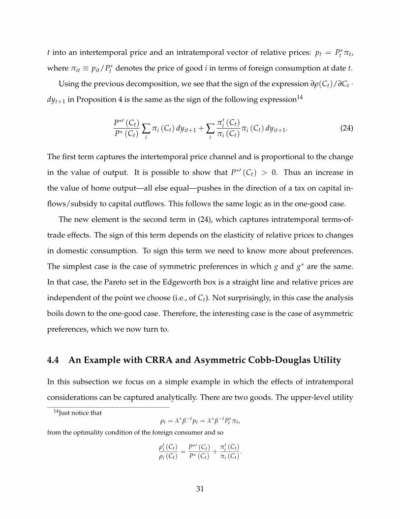
t into an intertemporal price and an intratemporal vector of relative prices: pt = P∗t πt,

where πit ≡ pit/P∗t denotes the price of good i in terms of foreign consumption at date t.

Using the previous decomposition, we see that the sign of the expression ∂ρ(Ct)/∂Ct ·dyt+1 in Proposition 4 is the same as the sign of the following expression14

P∗′ (Ct)

P∗ (Ct)∑

iπi (Ct) dyit+1 + ∑

i

π′i (Ct)

πi (Ct)πi (Ct) dyit+1. (24)

The first term captures the intertemporal price channel and is proportional to the change

in the value of output. It is possible to show that P∗′ (Ct) > 0. Thus an increase in

the value of home output—all else equal—pushes in the direction of a tax on capital in-

flows/subsidy to capital outflows. This follows the same logic as in the one-good case.

The new element is the second term in (24), which captures intratemporal terms-of-

trade effects. The sign of this term depends on the elasticity of relative prices to changes

in domestic consumption. To sign this term we need to know more about preferences.

The simplest case is the case of symmetric preferences in which g and g∗ are the same.

In that case, the Pareto set in the Edgeworth box is a straight line and relative prices are

independent of the point we choose (i.e., of Ct). Not surprisingly, in this case the analysis

boils down to the one-good case. Therefore, the interesting case is the case of asymmetric

preferences, which we now turn to.

4.4 An Example with CRRA and Asymmetric Cobb-Douglas Utility

In this subsection we focus on a simple example in which the effects of intratemporal

considerations can be captured analytically. There are two goods. The upper-level utility

14Just notice thatρt = λ∗β−t pt = λ∗β−tP∗t πt,

from the optimality condition of the foreign consumer and so

ρ′i (Ct)

ρi (Ct)=

P∗′ (Ct)

P∗ (Ct)+

π′i (Ct)

πi (Ct).

31

function at home is CRRA and the lower-level utility is Cobb-Douglas:

U (C) =1

1− γC1−γ, C = cα

1c1−α2 , (25)

where γ ≥ 0 and α > 1/2. Foreign utility functions take the same form, but the roles of

goods 1 and 2 are reversed

U∗ (C∗) =1

1− γ(C∗)1−γ , C∗ = (c∗2)

α (c∗1)1−α . (26)

Since α > 1/2, Home has a higher relative demand for good 1 in all periods. Without

risk of confusion, we now refer to good 1 and good 2 as Home’s “import-oriented” and

“export-oriented” sectors, respectively. The next proposition highlights how this distinc-

tion plays a key role in linking intertemporal and intratemporal terms-of-trade motives.15

Proposition 5 (Import- versus export-oriented growth) Suppose that equations (25)-(26) hold

with γ ≥ 0 and α > 1/2 and that between periods t and t + 1 there is a small change in the

home endowment dyt+1 = yt+1 − yt. If growth is import-oriented, dy1t+1 > 0 and dy2t+1 = 0,

it is optimal to tax capital inflows/subsidize capital outflows (θt < 0). Conversely, if growth is

export-oriented, dy1t = 0 and dy2t+1 > 0, it is optimal to tax capital inflows/subsidize capital

outflows (θt < 0) if and only if γ >(

2α−1α

) (P∗t C∗t

P∗t C∗t +PtCt

).

The idea behind the first part of Proposition 5 is closely related to Proposition 2. In

periods in which Home controls a larger fraction of the world endowment of good 1, the

incentive to subsidize consumption C increases. Here, however, the reason is twofold.

First, a larger endowment of good 1 means that Home is running a smaller (net) trade

deficit, which reduces the incentive to depress the intertemporal price P∗. Second, it

15Another simple example that can be solved analytically is the case of tradable and non-tradable goods.If there is only one tradable good, then Proposition 2 applies unchanged to changes in the endowment ofthe tradable good. The only difference between this case and the one-good case studied in Section 3 isthat taxes on capital inflows/subsidies on capital outflows (θt < 0) now are always accompanied by a realexchange rate appreciation, whereas taxes on capital outflows/subsidies on capital inflows (θt > 0) noware always accompanied by a real exchange rate depreciation.

32

means that within the period the country is selling more of good 1. Since home prefer-

ences are biased towards good 1, an increase in C drives up the intratemporal price of

good 1, which further increases the incentives to subsidize aggregate consumption.16

By contrast, when endowment growth is export-oriented, intertemporal and intratem-

poral considerations are not aligned anymore. If the elasticity of intertemporal substi-

tution, 1/γ, is low enough, the intertemporal motive for terms-of-trade manipulation

dominates and we get the same result as in the one good economy. If instead that elas-

ticity is high enough, the result goes in the opposite direction. Namely, it is possible that

when Home receives a larger endowment of good 2, it decides to subsidize aggregate

consumption less, even though the increase in y2 is reducing its (net) trade deficit. Intu-

itively, Home now benefits from reducing its own consumption since this increases the

intratemporal price of good 2 due again to the fact that, relative to foreign preferences,

home preferences are biased towards good 1. Proposition 5 formally demonstrates that

the intratemporal terms-of-trade motive is more likely to dominate the intertemporal one

if demand differences between countries are large and/or Foreign accounts for a large

share of world consumption.

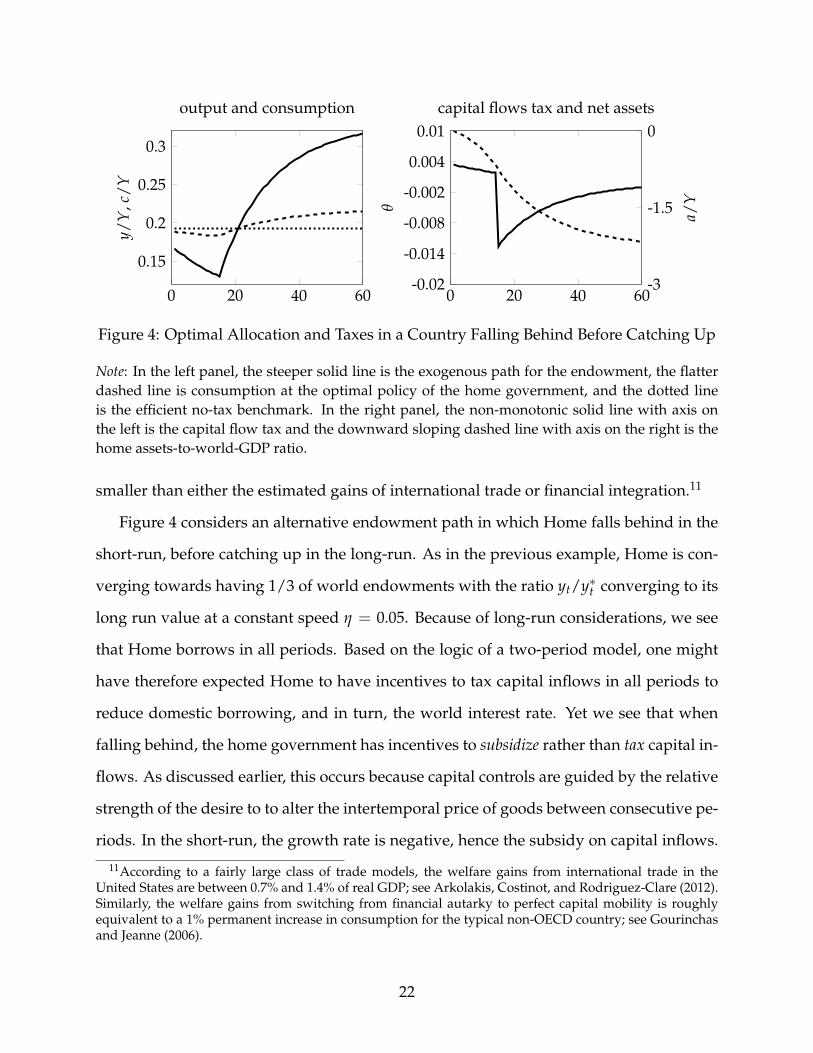
In order to illustrate the quantitative importance of this effect, we return to the exercise

presented in Section 3.3 in which Home is catching up with the rest of the world. For

simplicity, the world endowments of both goods are assumed to be constant over time. In

the first panel of Figure 5, the intertemporal elasticity of substitution is set to unity, γ = 1,

and demand differences are set such that α = 3/4. The bottom solid curve represents

the optimal tax on capital flows in the import-oriented scenario: the home endowment of

good 2 is fixed, but the home endowment of good 1 is 1/6 of world endowments at date 0

and is converging towards being 1/3 in the long run, with the ratio y1t/y∗1t converging to

its long run value at a constant speed η = 0.05. The top dashed curve instead represents

16Like in Section 3.1, whether Home is a net seller or a net buyer of good 1 does not matter per se. Whatmatters for the sign of optimal taxes is the fact that larger endowments of good 1 at date t + 1 imply thatHome tends to sell more (or buy less) of that good than at date t and, in turn, to benefit more (or to loseless) from an increase in the price of that good.

33

0 20 40 60-0.04

-0.02

0θ

γ = 1

0 20 40 60-0.04

-0.02

0

θ

γ = 0.33

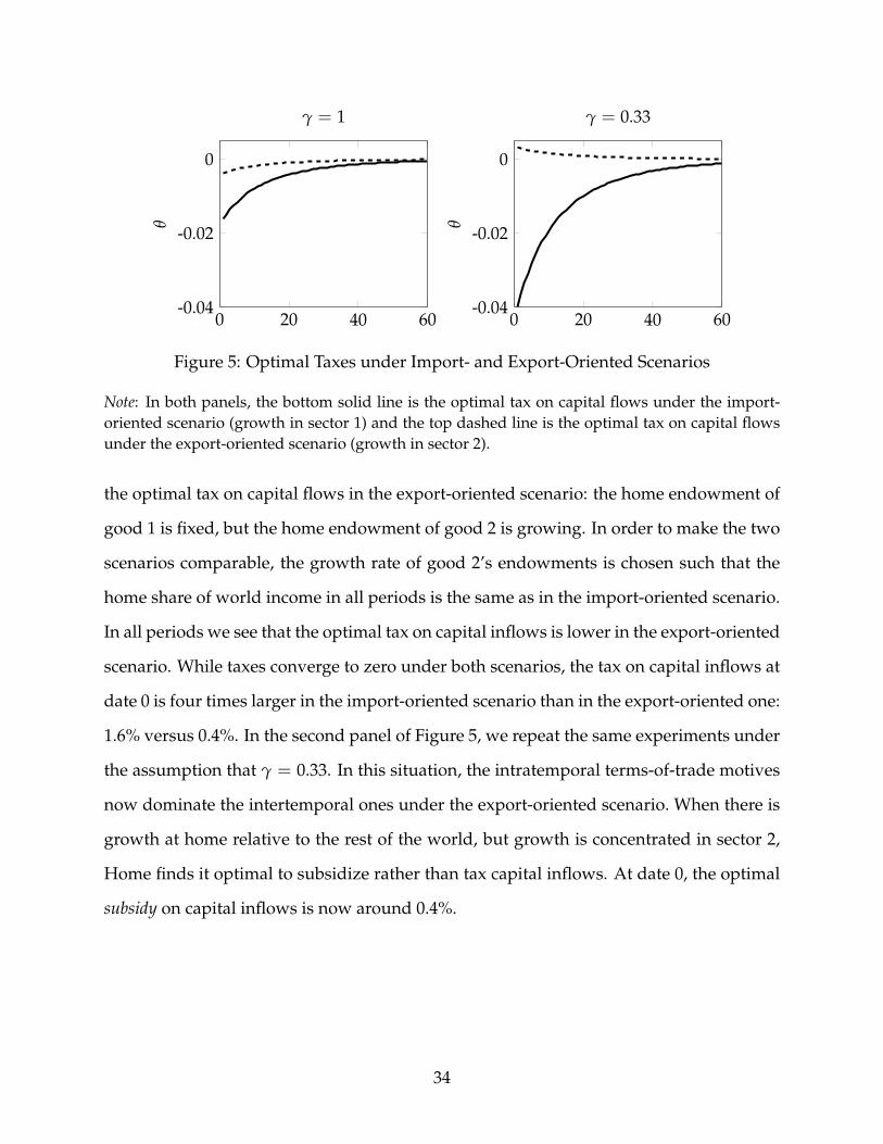
Figure 5: Optimal Taxes under Import- and Export-Oriented Scenarios

Note: In both panels, the bottom solid line is the optimal tax on capital flows under the import-oriented scenario (growth in sector 1) and the top dashed line is the optimal tax on capital flowsunder the export-oriented scenario (growth in sector 2).

the optimal tax on capital flows in the export-oriented scenario: the home endowment of

good 1 is fixed, but the home endowment of good 2 is growing. In order to make the two

scenarios comparable, the growth rate of good 2’s endowments is chosen such that the

home share of world income in all periods is the same as in the import-oriented scenario.

In all periods we see that the optimal tax on capital inflows is lower in the export-oriented

scenario. While taxes converge to zero under both scenarios, the tax on capital inflows at

date 0 is four times larger in the import-oriented scenario than in the export-oriented one:

1.6% versus 0.4%. In the second panel of Figure 5, we repeat the same experiments under

the assumption that γ = 0.33. In this situation, the intratemporal terms-of-trade motives

now dominate the intertemporal ones under the export-oriented scenario. When there is

growth at home relative to the rest of the world, but growth is concentrated in sector 2,

Home finds it optimal to subsidize rather than tax capital inflows. At date 0, the optimal

subsidy on capital inflows is now around 0.4%.

34

4.5 Capital Controls in a Small-Open Economy

In Section 3, the only motive for capital controls was the manipulation of world interest

rates. While such motive may be relevant for large countries, many small open economies

that use capital controls in practice are unlikely to have significant effects on world inter-

est rates. The goal of this final subsection is to illustrate how, because of the interaction

between intertemporal and intratemporal trade, terms-of-trade motives may still make

capital controls optimal for such economies.

Consider an economy with two goods. In line with the previous section, suppose

that the upper-level utility function at Home is CRRA and the lower-level utility is Cobb-

Douglas in both countries:

U (C) =1

1− γC1−γ, C = c1/2

1 c1/22 ,

U∗ (C∗) =N − 11− γ

(C∗)1−γ , C∗ =c∗1/N

1 c∗1−1/N2

N − 1,

where γ ≥ 0. World endowments of good 1 are equal to Y1, whereas world endowments

of good 2 are equal to NY2. One can think of this economy as the reduced-form of a

more general environment in which there are N countries in the world; each country is

endowed with a differentiated good; and each country spends a constant fraction of its

income on its own good as well as a CES aggregator of all goods in the world economy.

In the appendix we show that as N goes to infinity, i.e. as Home becomes a “small”

open economy, Home’s planning problem converges towards

max{Ct}

∞

∑t=0

βtU(Ct) (PS)

subject to∞

∑t=0

βtY−γ2

[g∗1(c

∗ (Ct))

g∗2(c∗ (Ct))(c1 (Ct)− y1t) + (c2 (Ct)− y2t)

]= 0, (27)

35

where g∗1(c∗ (Ct))/g∗2(c

∗ (Ct)) = Y2 +12

[C2

t /Y1 +√(

C2t /Y1

)2+ 4Y2

(C2

t /Y1)]

. In the

limit, aggregate consumption abroad, C∗t , converges towards Y2 in all periods, indepen-

dently of Home’s aggregate consumption decision. From the foreign consumer’s Euler

equation (23), the world real interest rate R∗t therefore converges towards R∗ = 1/β− 1 in

all periods. Accordingly, Home cannot manipulate its intertemporal terms-of-trade. Yet,

as equation (27) illustrates, Home can still manipulate its intratemporal temporal terms-

of-trade: g∗1(c∗ (Ct))/g∗2(c

∗ (Ct)) is strictly increasing in Home’s aggregate consumption,

Ct. As a result, Home will depart from perfect consumption smoothing along the opti-

mal path. Since departures from perfect consumption smoothing along the optimal path

can be implemented using taxes on capital flows, this establishes that in a neoclassical

benchmark model in which terms-of-trade manipulation is the only motive for capital

controls, even a country that cannot affect world interest rates may have incentives to tax

international capital flows.

In this example, a small-open economy accounts for an infinitesimal fraction of ag-

gregate consumption in every period. Thus it cannot affect intertemporal prices. Yet, it

always accounts for a signification fraction of the consumption of one of the two goods.

Thus it can, and will want to, affect intratemporal prices. If good specific trade taxes and

subsidies are prohibited by international agreements, capital controls offer an alternative

way to achieve that goal.

5 Capital Control Wars

In this section we go back to the one-good case, but consider the case in which both coun-

tries set capital controls optimally, taking as given the capital controls chosen by the other

country. As before, we assume that consumers can only trade one-period bonds on inter-

national capital markets, but we now let both the home and foreign government impose

proportional taxes θt and θ∗t , respectively, on the gross return on net asset position in inter-

36

national bond markets. At date 0, we assume that the two governments simultaneously

choose the sequences {θt} and {θ∗t } and commit to them. Given this assumption, we can

use the same primal approach developed in previous sections to offer a first look at the

outcome of capital control wars.17

5.1 Nash Equilibrium

We look for a Nash equilibrium, so we look at each government’s optimization problem

taking the other government’s tax sequence as given. Focusing on the problem of the

home government, the optimal taxes can be characterized in terms of a planning problem

involving directly the quantities consumed, as in the unilateral case. Given the sequence

{θ∗t } the foreign consumer’s Euler equation can be written as

u∗′(c∗t ) = β(1− θ∗t )(1 + rt)u∗′(c∗t+1). (28)

Since 1 + rt = pt/pt+1, a standard iterative argument then implies

pt = βt[∏t−1

s=0 (1− θ∗s )] [

p0u∗′(c∗t )/u∗′(c∗0)]

.

Accordingly, Home’s planning problem is now given by

max{ct}

∞

∑t=0

βtu(ct) (PN)

subject to∞

∑t=0

βtu∗′ (Y− ct)[∏t−1

s=0 (1− θ∗s )](ct − yt) = 0,

17The assumption of commitment is stronger here than in previous sections since it also precludes coun-tries to respond to the other country’s policies as they unfold over time. This de facto rules out any equi-librium in which governments may choose to cooperate along the equilibrium path, e.g., to have zero taxeson capital controls, by fear of being punished if they were to deviate from the equilibrium strategies. SeeDixit (1987) for an early discussion of related issues in a trade context.

37

where the new implementability constraint captures the fact that the home government

now takes foreign capital flow taxes as given. This yields the optimality condition

u′(ct) = µ[∏t−1

s=0 (1− θ∗s )] [

u∗′(c∗t )− u∗′′(c∗t )(ct − yt)]

, (29)

which further implies

u′(ct)

u′(ct+1)=

1(1− θ∗t )

u∗′(c∗t )− u∗′′(c∗t )(ct − yt)

u∗′(c∗t+1)− u∗′′(c∗t+1)(ct+1 − yt+1). (30)

From the domestic consumer’s Euler equation, we also know that

u′(ct) = β(1− θt)(1 + rt)u′(ct+1). (31)

Combining equations (30) and (31) with equation (28), we obtain after simplifications

1− θt =1− u∗′′(c∗t )

u∗′(c∗t )(ct − yt)

1− u∗′′(c∗t+1)

u∗′(c∗t+1)(ct+1 − yt+1)

.

The planning problem of the foreign government is symmetric. So the same logic implies

1− θ∗t =1− u′′(ct)

u′(ct)(c∗t − y∗t )

1− u′′(ct+1)u′(ct+1)

(c∗t+1 − y∗t+1).

Substituting for the foreign tax on international capital flows in equation (30) and using

the good market clearing condition (3), we obtain

u′(ct) + u′′(ct)(ct − yt)

u∗′(Y− ct)− u∗′′(Y− ct)(ct − yt)=

u′(ct+1) + u′′(ct+1)(ct+1 − yt+1)

u∗′(Y− ct+1)− u∗′′(Y− ct+1)(ct+1 − yt+1),

38

which can be rearranged as

u′(ct) + u′′(ct)(ct − yt)

u∗′(Y− ct)− u∗′′(Y− ct)(ct − yt)= α, for all t ≥ 0, (32)

where α ≡ [u′(c0) + u′′(c0)(c0 − y0)]/[u∗′(Y − c0) − u∗′′(Y − c0)(c0 − y0)] > 0. This is

the counterpart of equation (6) in Section 2. In particular, using equations (29) and (31)

and their counterparts in Foreign, one can check that α = λµ∗/λ∗µ, where λ and λ∗ are

the Lagrange multipliers associated with the intertemporal budget constraints in both

countries.

The next lemma provides sufficient conditions under which a Nash equilibrium exists.

Lemma 1 Suppose that the following conditions hold: (i) u and u∗ are twice continuously dif-

ferentiable, strictly increasing, and strictly concave, with limc→0 u′(c) = limc∗→0 u′(c∗) = ∞;

(ii) u′(ct)(ct − yt) and u∗′(c∗t )(c∗t − y∗t ) are strictly increasing and strictly concave in ct and c∗t ,

respectively, for all yt and y∗t ; and (iii) yt and y∗t are bounded away from zero for all t. Then a

Nash Equilibrium exists.

Compared to Section 3, the new condition being imposed is that u′(ct)(ct − yt) and

u∗′(c∗t )(c∗t − y∗t ) are strictly increasing in ct and c∗t , respectively. In the case of unilaterally

optimal capital controls, this condition necessarily holds locally; see equation (6). If not,

a country could simultaneously increase consumption and loosen the implementability

constraint. To establish existence of a Nash equilibrium we now require this condition to

hold globally. As we next demonstrate, this new condition and our previous assumptions

are also sufficient for consumption to be procyclical along the Nash equilibrium.

5.2 Main Results Revisited

Intuitively, one may expect that an increase in y would necessarily lead to an increase in c.

Indeed, we have established in Section 3 that if Home were to impose taxes unilaterally,

39

it would like to increase c in response to a positive shock in y. The same logic implies

that if Foreign were to impose taxes unilaterally, it would like to decrease c∗, i.e., to in-

crease c as well, in response to a positive shock in y. Thus both unilateral responses point

towards an increasing relationship between c and y. As the next lemma demonstrates, if

the assumptions of Lemma 1 are satisfied, the previous intuition is correct.

Lemma 2 Suppose that the assumptions of Lemma 1 hold. Then for any two periods t and s, if

the home endowment is larger in s, ys > yt, then the home consumption is also higher, cs > ct.

Using the procyclicality of consumption along the Nash equilibrium, we can use the

domestic and foreign consumer’s Euler equations to characterize capital control wars the

same way we characterized optimal capital controls in Section 3. Our main result about

capital control wars can be stated as follows.

Proposition 6 (Capital control wars) Suppose that the assumptions of Lemma 1 hold. Then along

the Nash equilibrium, the home and foreign capital flow taxes are such that:

1. Home interest rates are higher than foreign interest rates (θt < θ∗t ) if yt+1 > yt;

2. Home interest rates are lower than foreign interest rates (θt > θ∗t ) if yt+1 < yt;

3. Home and foreign interest rates are equal (θt = θ∗t ) if yt+1 = yt.

If there are no intertemporal distortions abroad, θ∗t = 0, then like in Section 3, an

increase in domestic endowments, yt+1 > yt, leads to a tax on capital inflows or a sub-

sidy to capital outflows, θt < 0, which is associated with higher domestic interest rates,

(1− θt) (1 + rt) > 1 + rt. In general, however, we cannot sign θt and θ∗t . The intuition for

this result is a combination of the intuition for the unilateral policy of Home and Foreign.

Suppose, for instance, that Home is running a trade deficit in period t. An increase in the

home endowment reduces the trade deficit and reduces the incentives of the home gov-

ernment to repress domestic consumption. Foreign incentives are symmetric, meaning

40

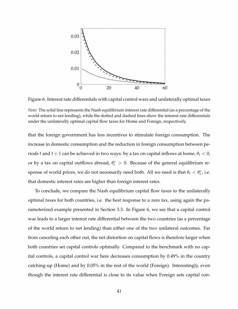
0 20 40 600

0.01

0.02

0.03

Figure 6: Interest rate differentials with capital control wars and unilaterally optimal taxes

Note: The solid line represents the Nash equilibrium interest rate differential (as a percentage of theworld return to net lending), while the dotted and dashed lines show the interest rate differentialsunder the unilaterally optimal capital flow taxes for Home and Foreign, respectively.

that the foreign government has less incentives to stimulate foreign consumption. The

increase in domestic consumption and the reduction in foreign consumption between pe-

riods t and t + 1 can be achieved in two ways: by a tax on capital inflows at home, θt < 0,

or by a tax on capital outflows abroad, θ∗t > 0. Because of the general equilibrium re-

sponse of world prices, we do not necessarily need both. All we need is that θt < θ∗t , i.e.

that domestic interest rates are higher than foreign interest rates.

To conclude, we compare the Nash equilibrium capital flow taxes to the unilaterally

optimal taxes for both countries, i.e. the best response to a zero tax, using again the pa-

rameterized example presented in Section 3.3. In Figure 6, we see that a capital control

war leads to a larger interest rate differential between the two countries (as a percentage

of the world return to net lending) than either one of the two unilateral outcomes. Far

from canceling each other out, the net distortion on capital flows is therefore larger when

both countries set capital controls optimally. Compared to the benchmark with no cap-

ital controls, a capital control war here decreases consumption by 0.49% in the country

catching-up (Home) and by 0.05% in the rest of the world (Foreign). Interestingly, even

though the interest rate differential is close to its value when Foreign sets capital con-

41

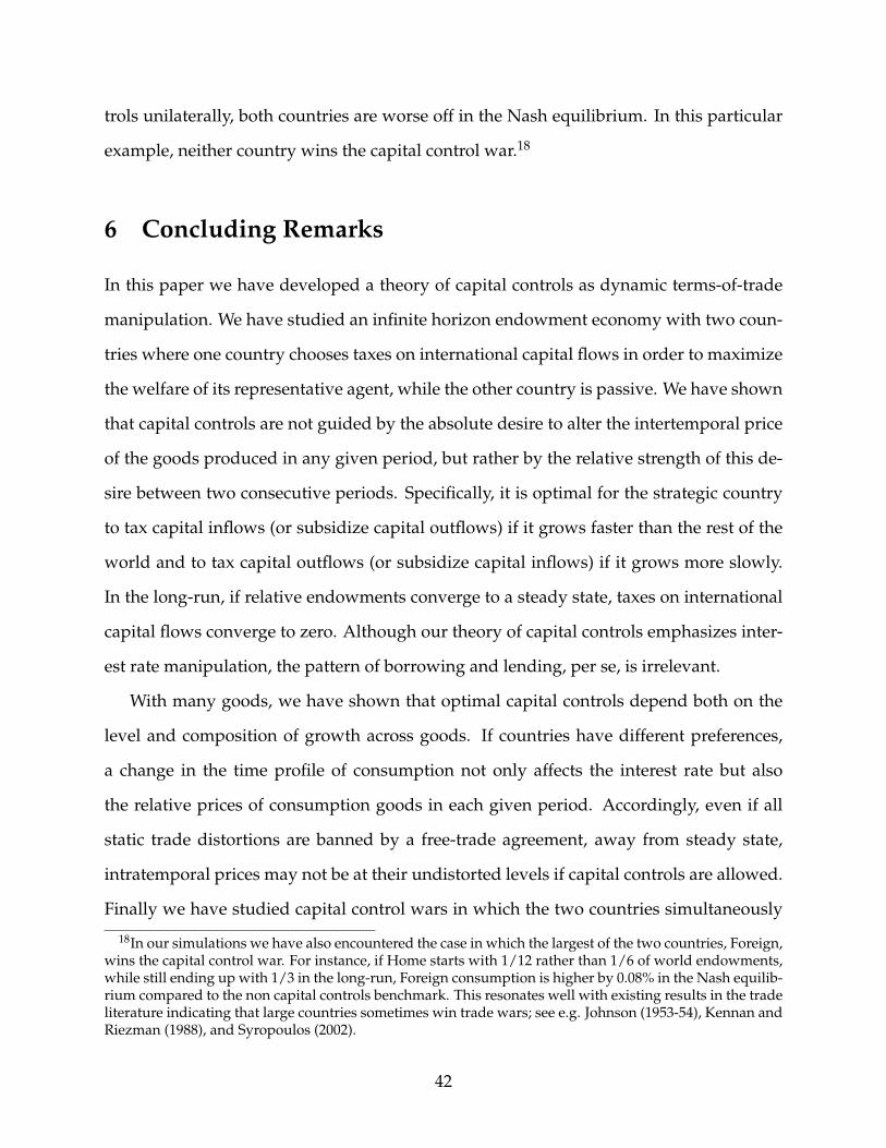
trols unilaterally, both countries are worse off in the Nash equilibrium. In this particular

example, neither country wins the capital control war.18

6 Concluding Remarks

In this paper we have developed a theory of capital controls as dynamic terms-of-trade

manipulation. We have studied an infinite horizon endowment economy with two coun-

tries where one country chooses taxes on international capital flows in order to maximize

the welfare of its representative agent, while the other country is passive. We have shown

that capital controls are not guided by the absolute desire to alter the intertemporal price

of the goods produced in any given period, but rather by the relative strength of this de-

sire between two consecutive periods. Specifically, it is optimal for the strategic country

to tax capital inflows (or subsidize capital outflows) if it grows faster than the rest of the

world and to tax capital outflows (or subsidize capital inflows) if it grows more slowly.

In the long-run, if relative endowments converge to a steady state, taxes on international

capital flows converge to zero. Although our theory of capital controls emphasizes inter-

est rate manipulation, the pattern of borrowing and lending, per se, is irrelevant.

With many goods, we have shown that optimal capital controls depend both on the

level and composition of growth across goods. If countries have different preferences,

a change in the time profile of consumption not only affects the interest rate but also

the relative prices of consumption goods in each given period. Accordingly, even if all

static trade distortions are banned by a free-trade agreement, away from steady state,

intratemporal prices may not be at their undistorted levels if capital controls are allowed.

Finally we have studied capital control wars in which the two countries simultaneously

18In our simulations we have also encountered the case in which the largest of the two countries, Foreign,wins the capital control war. For instance, if Home starts with 1/12 rather than 1/6 of world endowments,while still ending up with 1/3 in the long-run, Foreign consumption is higher by 0.08% in the Nash equilib-rium compared to the non capital controls benchmark. This resonates well with existing results in the tradeliterature indicating that large countries sometimes win trade wars; see e.g. Johnson (1953-54), Kennan andRiezman (1988), and Syropoulos (2002).

42

set taxes on capital flows. In the simple quantitative example that we consider, far from

canceling each other out, the net distortion on capital flows is larger than in the unilateral

case.

Our theory of capital controls is unapologetically normative. It does not try to ex-

plain the past behaviors of particular governments in Brazil, Malaysia, or China, whose

objectives may be far different from those assumed in this paper. Rather the goal of our

theory is to indicate what a government with the ability to manipulate interest rates and

other prices should do (at least from a unilateral perspective). Of course, this does not

imply that our theory has no practical implications for actual policy coordination efforts.

In the trade literature, optimal tariff arguments upon which the present analysis builds

have paved the way for a rich positive theory of international trade agreements; see Bag-

well and Staiger (2002). We hope that our analysis will provide a useful starting point

for thinking about agreements on capital controls as well as other related questions at the

frontier of international macro and international trade policy.

43

References

ANDERSON, J. E. (1991): “The Optimal Borrowing Tax,” Journal of International Economic

Integration, 6(1), 64–90.

ANDERSON, J. E., AND L. YOUNG (1992): “Optimal Taxation and Debt in an Open Econ-

omy,” Journal of Public Economics, 47, 27–57.

AOKI, K., G. BENIGNO, AND N. KIYOTAKI (2010): “Adjusting to Capital Account Liber-

alization,” C.E.P.R. Discussion Papers.

ARKOLAKIS, C., A. COSTINOT, AND A. RODRIGUEZ-CLARE (2012): “New Trade Models,

Same Old Gains?,” American Economic Review, 102(1), 94–130.

BAGWELL, K., AND R. W. STAIGER (1990): “A Theory of Managed Trade,” American Eco-

nomic Review, 80(4), 779–95.

BAGWELL, K., AND R. W. STAIGER (1999): “An Economic Theory of GATT,” American

Economic Review, 89(1), 215–248.

(2002): The Economics of the World Trading System. MIT Press.

(2011): “What Do Trade Negotiators Negotiate About? Empirical Evidence from

the World Trade Organization,” American Economic Review, 101(4), 1238–73.

BAIER, S. L., AND J. H. BERGSTRAND (2007): “Do free trade agreements actually increase

members’ international trade?,” Journal of International Economics, 71(1), 72–95.

BOND, E. W. (1990): “The Optimal Tariff Structure in Higher Dimensions,” International

Economic Review, 31(1), 103–16.

BRODA, C., N. LIMAO, AND D. E. WEINSTEIN (2008): “Optimal Tariffs and Market

Power: The Evidence,” American Economic Review, 98(5), 2032–65.

44

CABALLERO, R. J., AND G. LORENZONI (2007): “Persistent Appreciations and Overshoot-

ing: A Normative Analysis,” Working Paper 13077, National Bureau of Economic Re-

search.

CALVO, G. A., AND E. G. MENDOZA (2000): “Rational contagion and the globalization of

securities markets,” Journal of International Economics, 51(1), 79–113.

CHAMLEY, C. (1986): “Optimal Taxation of Capital in General Equilibrium,” Econometrica,

54, 607–22.

CHARI, V., AND P. J. KEHOE (1999): “Optimal fiscal and monetary policy,” in Handbook of

Macroeconomics, ed. by J. B. Taylor, and M. Woodford, pp. 1671–1745. Elsevier.

DIXIT, A. (1985): “Tax policy in open economies,” in Handbook of Public Economics, ed. by

A. J. Auerbach, and M. Feldstein, vol. 1 of Handbook of Public Economics, chap. 6, pp.

313–374. Elsevier.

DIXIT, A. K. (1987): “Strategic Aspects of Trade Policy,” in Advances in economic theory:

Fifth world congress, ed. by T. F. Bewley. Cambridge University Press, New York.

FEENSTRA, R. C. (1986): “Trade Policy with Several Goods and Market Linkages,” Journal

Of International Economics, 20(3-4), 249–267.

GOURINCHAS, P.-O., AND O. JEANNE (2006): “The Elusive Gains from International Fi-

nancial Integration,” Review of Economic Studies, 73(3), 715–741.

ITOH, M., AND K. KIYONO (1987): “Welfare-Enhancing Export Subsidies,” Journal of Po-

litical Economy, 95(1), 115–37.

JEANNE, O. (2011): “Capital Account Policies and the Real Exchange Rate,” Mimeo Johns

Hopkins University.

JEANNE, O., AND A. KORINEK (2010): “Excessive Volatility in Capital Flows: A Pigouvian

Taxation Approach,” American Economic Review, 100(2), 403–407.

45

JOHNSON, H. (1953-54): “Optimum Tariffs and Retaliation,” Review of Economic Studies, 1,

142–153.

JONES, R. W. (1967): “International Capital Movements and the Theory of Tariffs and

Trade,” Quarterly Journal of Economics, 81(1), 1–38.

JUDD, K. L. (1985): “Redistributive Taxation in a Perfect Foresight Model,” Journal of

Public Economics, 28, 59–83.

KENNAN, J., AND R. RIEZMAN (1988): “Do Big Countries Win Tariff Wars?,” International

Economic Review, 29(1), 81–85.

KEYNES, J. (1929): “The German transfer problem,” The Economic Journal, 39(153), 1–7.

KOSE, A., E. PRASAD, K. ROGOFF, AND S.-J. WEI (2009): “Financial Globalization: A

Reappraisal,” IMF Staff Papers, 56(1), 8–62.

LANE, P., AND G. M. MILESI-FERRETTI (2007): “The external wealth of nations mark II:

Revised and extended estimates of foreign assets and liabilities, 1970-2004,” Journal of

International Economics, 73, 223–250.

LUCAS, R., AND N. L. STOKEY (1983): “Optimal Fiscal and Monetary Policy in an Econ-

omy without Capital,” Journal of Monetary Economics, 12, 55–93.

LUENBERGER, D. G. (1969): Optimization by Vector Space Methods. John Wiley and Sons,

Inc.

MAGUD, N. E., C. M. REINHART, AND K. S. ROGOFF (2011): “Capital Controls: Myth

and Reality - A Portfolio Balance Approach,” Working Paper 16805, National Bureau of

Economic Research.

MARTIN, A., AND F. TADDEI (2010): “International Capital Flows and Credit Market Im-

perfections: a Tale of Two Frictions,” Collegio Carlo Alberto.

46

MCKINNON, R. I., AND W. E. OATES (1966): “The Implications of International Economic

Integration for Monetary, Fiscal, and Exchange-Rate Policy,” Princeton Studies in Inter-

national Finance.

MILL, J. (1844): Essays on Some Unsettled Questions of Political Economy. London: Parker.

OBSTFELD, M., AND K. S. ROGOFF (1996): Foundations of International Macroeconomics. The

MIT Press.

OBSTFELD, M., J. C. SHAMBAUGH, AND A. M. TAYLOR (2010): “Financial Stability, the

Trilemma, and International Reserves,” American Economic Journal: Macroeconomics,

2(2), 57–94.

OHLIN, B. (1929): “The reparation problem: a discussion,” Economic Journal, 39(154), 172–

182.

OSTRY, J. D., A. R. GHOSH, K. HABERMEIER, M. CHAMON, M. S. QURESHI, AND D. B.

REINHARDT (2010): “Capital Inflows: The Role of Controls,” IMF Staff Position Note.

STAIGER, R. W. (1995): “International rules and institutions for trade policy,” in Handbook

of International Economics, ed. by G. M. Grossman, and K. Rogoff, vol. 3. Elsevier.

STIGLITZ, J. E. (1976): “Monopoly and the Rate of Extraction of Exhaustible Resources,”

American Economic Review, 66(4), 655–61.

SUBRAMANIAN, A., AND S.-J. WEI (2007): “The WTO promotes trade, strongly but un-

evenly,” Journal of International Economics, 72(1), 151–175.

SYROPOULOS, C. (2002): “Optimum Tariffs and Retaliation Revisited: How Country Size

Matters,” Review of Economic Studies, 69(3), 707–27.

TORRENS, R. (1844): The Budget: On Commercial Policy and Colonial Policy. London: Smith,

Elder.

47

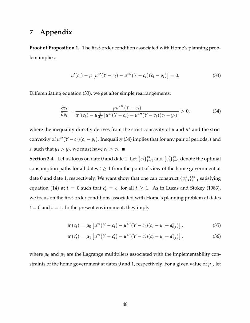
7 Appendix

Proof of Proposition 1. The first-order condition associated with Home’s planning prob-

lem implies:

u′(ct)− µ[u∗′(Y− ct)− u∗′′(Y− ct)(ct − yt)

]= 0. (33)

Differentiating equation (33), we get after simple rearrangements:

∂ct

∂yt=

µu∗′′ (Y− ct)

u′′(ct)− µ ∂∂ct

[u∗′(Y− ct)− u∗′′(Y− ct)(ct − yt)]> 0, (34)

where the inequality directly derives from the strict concavity of u and u∗ and the strict

convexity of u∗′(Y− ct)(ct− yt). Inequality (34) implies that for any pair of periods, t and

s, such that ys > yt, we must have cs > ct.

Section 3.4. Let us focus on date 0 and date 1. Let {ct}∞t=1 and {c′t}∞

t=1 denote the optimal

consumption paths for all dates t ≥ 1 from the point of view of the home government at

date 0 and date 1, respectively. We want show that one can construct {a∗1,s}∞s=1 satisfying

equation (14) at t = 0 such that c′t = ct for all t ≥ 1. As in Lucas and Stokey (1983),

we focus on the first-order conditions associated with Home’s planning problem at dates

t = 0 and t = 1. In the present environment, they imply

u′(ct) = µ0[u∗′(Y− ct)− u∗′′(Y− ct)(ct − yt + a∗0,t)

], (35)

u′(c′t) = µ1[u∗′(Y− c′t)− u∗′′(Y− c′t)(c

′t − yt + a∗1,t)

], (36)

where µ0 and µ1 are the Lagrange multipliers associated with the implementability con-

straints of the home government at dates 0 and 1, respectively. For a given value of µ1, let

48

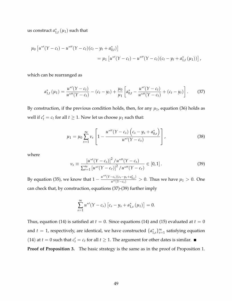
us construct a∗1,t (µ1) such that

µ0[u∗′(Y− ct)− u∗′′(Y− ct)(ct − yt + a∗0,t)

]= µ1

[u∗′(Y− ct)− u∗′′(Y− ct)(ct − yt + a∗1,t (µ1))

],

which can be rearranged as

a∗1,t (µ1) =u∗′(Y− ct)

u∗′′(Y− ct)− (ct − yt) +

µ0

µ1

[a∗0,t −

u∗′(Y− ct)

u∗′′(Y− ct)+ (ct − yt)

]. (37)

By construction, if the previous condition holds, then, for any µ1, equation (36) holds as

well if c′t = ct for all t ≥ 1. Now let us choose µ1 such that:

µ1 = µ0

∞

∑s=1

νs

1−u∗′′(Y− cs)

(cs − ys + a∗0,s

)u∗′(Y− cs)

, (38)

where

νs ≡[u∗′(Y− cs)]

2 /u∗′′(Y− cs)

∑∞r=1 [u∗′(Y− cr)]

2 /u∗′′(Y− cr)∈ [0, 1] . (39)

By equation (35), we know that 1− u∗′′(Y−cs)(cs−ys+a∗0,s)

u∗′(Y−cs)> 0. Thus we have µ1 > 0. One

can check that, by construction, equations (37)-(39) further imply

∞

∑s=1

u∗′(Y− cs)[cs − ys + a∗1,s (µ1)

]= 0.

Thus, equation (14) is satisfied at t = 0. Since equations (14) and (15) evaluated at t = 0

and t = 1, respectively, are identical, we have constructed {a∗1,s}∞s=1 satisfying equation

(14) at t = 0 such that c′t = ct for all t ≥ 1. The argument for other dates is similar.

Proof of Proposition 3. The basic strategy is the same as in the proof of Proposition 1.

49

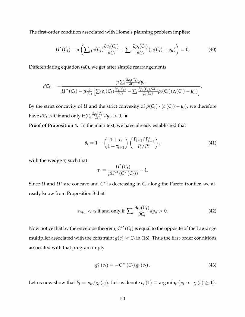
The first-order condition associated with Home’s planning problem implies:

U′ (Ct)− µ

(∑i ρi(Ct)

∂ci(Ct)

∂Ct+ ∑i

∂ρi(Ct)

∂Ct(ci(Ct)− yit)

)= 0, (40)

Differentiating equation (40), we get after simple rearrangements

dCt = −µ ∑i

∂ρi(Ct)∂Ct

dyit

U′′ (Ct)− µ ∂∂Ct

[∑i ρi(Ct)

∂ci(Ct)∂Ct−∑i

∂ρi(Ct)/∂Ctρi(Ct)

ρi(Ct)(ci(Ct)− yit)] .

By the strict concavity of U and the strict convexity of ρ(Ct) · (c (Ct)− yt), we therefore

have dCt > 0 if and only if ∑i∂ρi(Ct)

∂Ctdyit > 0.

Proof of Proposition 4. In the main text, we have already established that

θt = 1−(

1 + τt

1 + τt+1

)(Pt+1/P∗t+1

Pt/P∗t

), (41)

with the wedge τt such that

τt =U′ (Ct)

µU∗′ (C∗ (Ct))− 1.

Since U and U∗ are concave and C∗ is decreasing in Ct along the Pareto frontier, we al-

ready know from Proposition 3 that

τt+1 < τt if and only if ∑i∂ρi(Ct)

∂Ctdyit > 0. (42)

Now notice that by the envelope theorem, C∗′ (Ct) is equal to the opposite of the Lagrange

multiplier associated with the constraint g(c) ≥ Ct in (18). Thus the first-order conditions

associated with that program imply

g∗i (ct) = −C∗′ (Ct) gi (ct) . (43)

Let us now show that Pt = pit/gi (ct). Let us denote ct (1) ≡ arg minc {pt · c : g (c) ≥ 1}.

50

The associated first-order conditions are given by (i) pi = λgi [ct (1)] and (ii) g [ct (1)] =

1. This implies

Pt = ∑i pitcit (1) = λ ∑i gi [ct (1)] cit (1) = λg [ct (1)] = λ,

where the third equality uses the fact that g is homogeneous of degree one. Combining

this equality with condition (i), we obtain Pt = pit/gi [ct (1)]. Since gi is homogeneous

of degree zero, this further implies Pt = pit/gi (ct) for all i = 1, ..., n. The same logic

applied to Foreign implies P∗t = pit/g∗i (ct). Combining the two previous observations

with equation (43), we obtainPt

P∗t= −C∗′ (Ct) .

Since g and g∗ are concave and homogeneous of degree one, standard arguments imply

that the solution C∗ of (18) is (weakly) concave in Ct. By Proposition 3, we therefore have

Pt+1/P∗t+1 > Pt/P∗t if and only if ∑i

∂ρi(Ct)

∂Ctdyit > 0. (44)

Combining equation (41) with conditions (42) and (44), we finally get θt < 0 if and only if

∑i∂ρi(Ct)

∂Ctdyit > 0.

Proof of Proposition 5. Suppose that dyit+1 > 0 and dyjt+1 = 0. By Proposition 4, we

know that θt < 0 if and only if ∂ρ(Ct)/∂Ct · dyt+1 > 0, where ρ(Ct) ≡ U∗′ (C∗(Ct))∇g∗(c∗ (Ct)).

Thus if dyit+1 > 0 and dyjt+1 = 0, θt < 0 if and only if

U∗′′ (C∗(Ct))

U∗′ (C∗(Ct))

∂C∗(Ct)

∂Ct+

[g∗ii(c

∗ (Ct))

g∗i (c∗ (Ct))

∂c∗i (Ct)

∂Ct+

g∗ij(c∗ (Ct))

g∗i (c∗ (Ct))

∂c∗j (Ct)

∂Ct

]> 0. (45)

Consider the first term on the left-hand side of inequality (45). In the proof of Proposition

4, we have already established that

∂C∗(Ct)

∂Ct= − Pt

P∗t.

51

Since U∗ (C∗) = 11−γ (C∗)1−γ, we therefore have

U∗′′ (C∗(Ct))

U∗′ (C∗(Ct))

∂C∗(Ct)

∂Ct=

γPt

P∗t C∗t. (46)

Let us now turn to the second term on the left-hand side of inequality (45). Our goal is to

establish that

g∗11(c∗t )

g∗1(c∗t )

∂c∗1(Ct)

∂Ct+

g∗12(c∗t )

g∗1(c∗t )

∂c∗2(Ct)

∂Ct=

α

(1− α)Ct

(2α− 1) c2 (Ct)

(1− α) c∗2 (Ct) + αc2 (Ct), (47)

g∗12(c∗t )

g∗2(c∗t )

∂c∗1(Ct)

∂Ct+

g∗22(c∗t )

g∗2(c∗t )

∂c∗2(Ct)

∂Ct= − 1

Ct

(2α− 1) c2 (Ct)

(1− α) c∗2 (Ct) + αc2 (Ct). (48)

Since g∗(c∗) = (c∗2)α (c∗1)

1−α, simple algebra implies

g∗11(c∗t )

g∗1(c∗t )

= − α

c∗1t,

g∗12(c∗t )

g∗1(c∗t )

=α

c∗2t,

g∗12(c∗t )

g∗2(c∗t )

=(1− α)

c∗1t,

g∗22(c∗t )

g∗2(c∗t )

= − (1− α)

c∗2t.

Using the previous expressions, we obtain

g∗11(c∗t )

g∗1(c∗t )

∂c∗1(Ct)

∂Ct+

g∗12(c∗t )

g∗1(c∗t )

∂c∗2(Ct)

∂Ct= α

∂ ln [c∗2(Ct)/c∗1(Ct)]

∂Ct, (49)

g∗12(c∗t )

g∗2(c∗t )

∂c∗1(Ct)

∂Ct+

g∗22(c∗t )

g∗2(c∗t )

∂c∗2(Ct)

∂Ct= − (1− α)

∂ ln [c∗2(Ct)/c∗1(Ct)]

∂Ct. (50)

Let us compute∂ ln[c∗2(Ct)/c∗1(Ct)]

∂Ct. By definition, c (Ct) and c∗ (Ct) are the solution of

maxc,c∗

(c∗2)α (c∗1)

1−α

52

subject to

c1 + c∗1 ≤ Y1,

c2 + c∗2 ≤ Y2,

cα1c1−α

2 ≥ Ct.

The associated first-order conditions imply

c∗2 (Ct)

c∗1 (Ct)= β

(Y2 − c∗2 (Ct)

Y1 − c∗1 (Ct)

)with β ≡ [α/(1− α)]2 , (51)

andY2 − c∗2 (Ct)

Y1 − c∗1 (Ct)=

(Ct

Y2 − c∗2 (Ct)

)− 1α

. (52)

Combining the two previous expressions, we obtain

∂ ln [c∗2(Ct)/c∗1(Ct)]

∂Ct= −1

α

(1Ct− ∂ ln [Y2 − c∗2(Ct)]

∂Ct

)= −1

α

(1Ct− ∂ ln [c2(Ct)]

∂Ct

). (53)

Let us compute ∂ ln[c2(Ct)]∂Ct

. Using the resource constraint, we can express equation (51) as

c1 (Ct) =βc2 (Ct)Y1

Y2 − (1− β) c2 (Ct).

Together with equation (52), using again the resource constraint, this implies

c2 (Ct) = Ct

[Y2 − (1− β) c2 (Ct)

βY1

]α

.

Taking the log and differentiating, we obtain after rearrangements

∂ ln [c2(Ct)]

∂Ct=

Y2 − (1− β) c2 (Ct)

Ct [Y2 − (1− α) (1− β) c2 (Ct)]. (54)

53

Equations (53) and (54) imply

∂ ln [c∗2(Ct)/c∗1(Ct)]

∂Ct=

1Ct

(β− 1) c2 (Ct)

Y2 + (1− α) (β− 1) c2 (Ct).

Using the definition of β ≡ [α/(1− α)]2, we can rearrange the previous expression as

∂ ln [c∗2(Ct)/c∗1(Ct)]

∂Ct=

1(1− α)Ct

(2α− 1) c2 (Ct)

(1− α) c∗2 (Ct) + αc2 (Ct).

Equations (47) and (48) directly derive from the previous expression and equations (49)

and (50), respectively.

To conclude the proof of Proposition 5, first note that equations (46) and (47) imply

U∗′′ (C∗(Ct))

U∗′ (C∗(Ct))

∂C∗(Ct)

∂Ct+

[g∗11(c

∗t )

g∗1(c∗t )

∂c∗1(Ct)

∂Ct+

g∗12(c∗t )

g∗1(c∗t )

∂c∗2(Ct)

∂Ct

]=

γPt

P∗t C∗t+

α

(1− α)Ct

(2α− 1) c2 (Ct)

(1− α) c∗2 (Ct) + αc2 (Ct)> 0.

Thus if dy1t+1 > 0 and dy2t+1 = 0, then θt < 0. Second note that equations (46) and (48)

imply

U∗′′ (C∗(Ct))

U∗′ (C∗(Ct))

∂C∗(Ct)

∂Ct+

[g∗12(c

∗t )

g∗2(c∗t )

∂c∗1(Ct)

∂Ct+

g∗22(c∗t )

g∗2(c∗t )

∂c∗2(Ct)

∂Ct

]=

γPt

P∗t C∗t− 1

Ct

(2α− 1) c2 (Ct)

(1− α) c∗2 (Ct) + αc2 (Ct).

According to this expression, if dy1t+1 = 0 and dy2t+1 > 0, then θt < 0 if and only if

γ >P∗t C∗tPtCt

(2α− 1) c2 (Ct)

(1− α) c∗2 (Ct) + αc2 (Ct). (55)

Since utility functions are Cobb-Douglas, g(c) = cα1c1−α

2 and g∗(c∗) = (c∗2)α (c∗1)

1−α, we

54

know that

p2tc2 (Ct) = (1− α) PtCt

p2tc∗2 (Ct) = αP∗t C∗t

Combining these two observations with inequality (55), we conclude that if dy1t+1 = 0

and dy2t+1 > 0, then θt < 0 if and only if γ >(

2α−1α

) (P∗t C∗t

P∗t C∗t +PtCt

).

Section 4.5. Consider first the Pareto Problem. By definition, c (Ct) and c∗ (Ct) solve

maxc,c∗

c∗1/N1 c∗1−1/N

2

subject to

c1 + c∗1 ≤ Y1,

c2 + c∗2 ≤ Y2N,

c1/21 c1/2

2 ≥ Ct.

The associated first-order conditions imply

c∗2c∗1

= (N − 1)(NY2 − c∗2)(

Y1 − c∗1) ,

(Y1 − c∗1)1/2 (NY2 − c∗2)

1/2 = Ct.

Combining these two expressions we get

(c∗2)2 +

[(N − 2)C2

t(N − 1)Y1

− 2NY2

]c∗2 +

[(NY2)

2 − N(

Y2

Y1

)C2

t

]= 0.

55

This implies

c∗2 (Ct) = NY2 −12

(N − 2)C2t

(N − 1)Y1+

√[(N − 2)C2

t(N − 1)Y1

]2

+ 4(

NN − 1

)(Y2

Y1

)C2

t

.

In turn, we obtain

c∗1 (Ct) =

NY2 − 12

{(N−2)C2

t(N−1)Y1

+

√[(N−2)C2

t(N−1)Y1

]2+ 4

( NN−1

) (Y2Y1

)C2

t

}

NY2 +(N−2)

2

{(N−2)C2

t(N−1)Y1

+

√[(N−2)C2

t(N−1)Y1

]2+ 4

( NN−1

) (Y2Y1

)C2

t

} .

Using the two previous expressions, we can compute

C∗ (Ct) =(

NN − 1

)Y2 −

12 (N − 1)

(N − 2)C2t

(N − 1)Y1+

√[(N − 2)C2

t(N − 1)Y1

]2

+ 4(

NN − 1

)(Y2

Y1

)C2

t

×

NY2 +(N − 2)

2

(N − 2)C2t

(N − 1)Y1+

√[(N − 2)C2

t(N − 1)Y1

]2

+ 4(

NN − 1

)(Y2

Y1

)C2

t

−1/N

,

(N − 1) g∗1(c∗ (Ct)) =

1N

NY2 +(N − 2)

2

(N − 2)C2t

(N − 1)Y1+

√[(N − 2)C2

t(N − 1)Y1

]2

+ 4(

NN − 1

)(Y2

Y1

)C2

t

1−1/N

,

and

(N − 1) g∗2(c∗ (Ct)) =(

1− 1N

)NY2 +(N − 2)

2

(N − 2)C2t

(N − 1)Y1+

12

√[(N − 2)C2

t(N − 1)Y1

]2

+ 4(

NN − 1

)(Y2

Y1

)C2

t

−1/N

.

56

As N goes to infinity, we therefore get

limN→∞

C∗ (Ct) = Y2,

limN→∞

(N − 1) g∗1(c∗ (Ct)) = Y2 +

12

C2t

Y1+

√(C2

tY1

)2

+ 4(

Y2

Y1

)C2

t

,

limN→∞

(N − 1) g∗2(c∗ (Ct)) = 1.

As N goes to infinity the constraint (19) associated with Home’s planning problem there-

fore converges towards

∞

∑t=0

βtY−γ2

[g∗1(c

∗ (Ct))

g∗2(c∗ (Ct))(c1 (Ct)− y1t) + (c2 (Ct)− y2t)

]= 0,

where g∗1(c∗ (Ct))/g∗2(c

∗ (Ct)) = Y2 +12

[C2

t /Y1 +√(

C2t /Y1

)2+ 4Y2

(C2

t /Y1)]

.

Proof of Lemma 1. A Nash equilibrium corresponds to a pair of sequences of taxes on

one-period bonds, (θ ≡ {θt} , θ∗ ≡ {θ∗t }), such that

θ ∈ arg maxθ

{∞

∑t=0

βtu(ct(θ, θ∗

))|

∞

∑t=0

pt(θ, θ∗

)(ct(θ, θ∗

)− yt) = 0

}, (56)

θ∗ ∈ arg maxθ∗

{∞

∑t=0

βtu∗(c∗t(θ, θ∗

))|

∞

∑t=0

pt(θ, θ∗

)(c∗t(θ, θ∗

)− y∗t ) = 0

}, (57)

where the pair of consumption sequences, (c (θ, θ∗) ≡ {ct (θ, θ∗)} , c∗ (θ, θ∗) ≡ {c∗t (θ, θ∗)}),and the sequence of prices, p (θ, θ∗) ≡ {pt (θ, θ∗)}, are such that consumers maximize

their utility in both countries,

c (θ, θ∗) ∈ arg maxc

{∞

∑t=0

βtu(ct)|∞

∑t=0

pt (θ, θ∗)

∏t−1s=0 (1− θs)

(ct − yt) = L (θ, θ∗)

}, (58)

c∗ (θ, θ∗) ∈ arg maxc∗

{∞

∑t=0

βtu∗(c∗t )|∞

∑t=0

pt (θ, θ∗)

∏t−1s=0 (1− θ∗s )

(c∗t − y∗t ) = L∗ (θ, θ∗)

}, (59)

57

and markets clear in every period,

ct (θ, θ∗) + c∗t (θ, θ∗) = Y, (60)

with L (θ, θ∗) and L∗ (θ, θ∗) the total tax revenues in Home and Foreign, respectively.

In this proof, we will first focus on the following primal problems:

c ∈ arg maxc

{∞

∑t=0

βtu(ct)|∞

∑t=0

βtu∗′ (Y− ct)[∏t−1

s=0 (1− θ∗s )](ct − yt) = 0

}, (61)

c∗ ∈ arg maxc∗

{∞

∑t=0

βtu∗(c∗t )|∞

∑t=0

βtu′ (Y− c∗t )[∏t−1

s=0 (1− θs)](c∗t − y∗t ) = 0

}, (62)

for some guessed sequences of taxes, (θ, θ∗), and show that there exists consumption

sequences, (c, c∗), that solves the primal problems, (61) and (62). We will then verify that

if (c, c∗) solves the primal problems, (61) and (62), then (θ, θ∗) is a Nash equilibrium that

solves (56) and (57). We proceed in four steps.

Step 1: For any α > 0 and y ∈ (0, Y), there exists a unique c(α, y) such that

u′(c) + u′′(c)(c− y)u∗′(Y− c)− u∗′′(Y− c)(c− y)

= α. (63)

Furthermore c(α, y) is continuous, strictly decreasing in α, and strictly increasing in y.

To see this, first note that Conditions (i) and (ii) imply that u′(c) + u′′(c)(c − y) >

0, u∗′(Y − c) − u∗′′(Y − c)(c − y) > 0, u′(c) + u′′(c)(c − y) is continuous and strictly

decreasing in c, and u∗′(Y − c)− u∗′′(Y − c)(c− y) is continuous and strictly increasing

in c. This further implies that F(c, y) ≡ u′(c)+u′′(c)(c−y)u∗′(Y−c)−u∗′′(Y−c)(c−y) is continuous and strictly

decreasing in c. From Conditions (i) and (iii), we also know that

limc→0

u′(c) + u′′(c)(c− y) ≥ limc→0

u′(c) = ∞,

limc→Y

u∗′(Y− c)− u∗′′(Y− c)(c− y) ≥ limc∗→0

u∗′(c∗) = ∞,

58

which implies limc→0 F(c, y) = ∞ and limc→Y F(c, y) = 0. By the Intermediate Value

Theorem, for any α > 0, there therefore exists c(α, y) such that equation (63) holds. Fur-

thermore since F is strictly decreasing in c, c(α, y) is unique, continuous, and strictly de-

creasing in α. Finally since F(c, y) is continuous and strictly increasing in y, by the strict

concavity of u and u∗, c(α, y) must be continuous and strictly increasing in y.

Step 2: For any sequence {yt}, there exists α0 > 0 such that

∞

∑t=0

βtu∗′(

Y− c(

α0, yt

)) [∏t−1

s=0

(1− θ∗s

(α0))]

(c(

α0, yt

)− yt) = 0, (64)

∞

∑t=0

βtu′(

c(

α0, yt

)) [∏t−1

s=0

(1− θs

(α0))]

(yt − c(

α0, yt

)) = 0, (65)

with the sequences {θt (α)} and {θ∗t (α)} constructed such that

1− θt (α) =1− u∗′′(Y−c(α,yt))

u∗′(Y−c(α,yt))(c (α, yt)− yt)

1− u∗′′(Y−c(α,yt+1))u∗′(Y−c(α,yt+1))

(c (α, yt+1)− yt+1), (66)

1− θ∗t (α) =1− u′′(c(α,yt))

u′(c(α,yt))(yt − c (α, yt))

1− u′′(c(α,yt+1))u′(c(α,yt+1))

(yt+1 − c (α, yt+1)). (67)

Using equation (67), we can rearrange equation (64) as

∞

∑t=0

βtu∗′ (Y− c (α, yt))u∗′ (Y− c (α, yt)) (c (α, yt)− yt)

u∗′ (Y− c (α, yt))− u∗′′(Y− c (α, yt))(c (α, yt)− yt)= 0.

Let us denote

g (α, yt) ≡ u∗′ (Y− c (α, yt))u∗′ (Y− c (α, yt)) (c (α, yt)− yt)

u∗′ (Y− c (α, yt))− u∗′′(Y− c (α, yt))(c (α, yt)− yt).

We know that u∗′ (Y− c), u∗′ (Y− c) (c − yt), and u∗′ (Y− c) − u∗′′(Y − c)(c − yt) > 0

are continuous functions of c. Thus u∗′ (Y− c) u∗′(Y−c)(c−yt)u∗′(Y−c)−u∗′′(Y−c)(c−yt)

is continuous in c.

Since c (α, yt) is continuous in α for all yt by Step 1, g (α, yt) is continuous in α. Similarly,

59

u∗′ (Y− c) (c− yt) and u∗′ (Y− c)− u∗′′(Y − c)(c− yt) > 0 are continuous functions of

yt. Thus u∗′ (Y− c) u∗′(Y−c)(c−yt)u∗′(Y−c)−u∗′′(Y−c)(c−yt)

is continuous in yt. Since c (α, yt) is continuous

in yt for all α by Step 1, g (α, yt) is continuous in yt.

By Condition (iii), there exists ε > 0 such that yt ∈ [ε, Y− ε] for all t. By equation (63)

and the boundary condition limc∗→0 u∗′(c∗) = ∞, we know that, for any y ∈ [ε, Y− ε],

limα→0 c (α, y) = Y. Thus there must exist α > 0 such that c (α, ε) > Y − ε. By equa-

tion (63) and the boundary condition limc→0 u′(c) = ∞, we also know that, for any

y ∈ [ε, Y− ε], limα→∞ c (α, y) = 0. Thus there must exist α > 0 such that c (α, Y− ε) < ε.

Since c (α, y) is increasing in y by Step 1, we must therefore have c (α, y) > Y − ε and

c (α, y) < ε for all y ∈ [ε, Y− ε]. Furthermore since c (α, y) is decreasing in α by Step 1 and

c (α, ε) < c (α, Y− ε) < ε < Y− ε < c (α, ε), we must have α > α.

Let us now restrict ourselves to α ∈ [α, α]. Since g (α, yt) is continuous in (α, yt), there

must exist M > 0 such that |g (α, yt) | ≤ M for all (α, y) ∈ [α, α]× [ε, Y− ε]. We therefore

have |βtg (α, yt) | ≤ Mβt for all α ∈ [α, α] and all t. By Weierstrass criterion, GT (α) ≡

∑Tt=0 βtg (α, yt) therefore converges uniformly towards G∞ (α) ≡ ∑∞

t=0 βtg (α, yt). And by

the uniform convergence theorem and the continuity of βtg (α, yt) in α for all t, G∞ (α)

must be continuous in α. By construction of α and α, we have βtg (α, yt) > 0 for all t and

βtg (α, yt) < 0 for all t. Thus G∞ (α) > 0 and G∞ (α) < 0. Since G∞ (α) is continuous in α,

the Intermediate Value Theorem implies the existence of α0 such that equation (64) holds.

To conclude one can use equations (63), (66), and (67) to check that if equation (64)

holds, then equation (65) holds as well.

Step 3: For any sequence {yt},{

c(α0, yt

)}and

{Y− c

(α0, yt

)}are a solution of the primal

problems, (61) and (62), for {θs} ≡{

θs(α0)} and {θ∗s } ≡

{θ∗s(α0)}.

Let us first show that there exists µ > 0 such that for all t,

u′(c(

α0, yt

)) = µ

[∏t−1

s=0

(1− θ∗s

(α0))] [

u∗′(Y− c(

α0, yt

))− u∗′′(Y− c

(α0, yt

))(c(

α0, yt

)− yt)

](68)

60

By construction of {θ∗ (α)}, we know that for any α:

1− θ∗t (α) =1− u′′(c(α,yt))

u′(c(α,yt))(yt − c (α, yt))

1− u′′(c(α,yt+1))u′(c(α,yt+1))

(yt+1 − c (α, yt+1)).

Thus [∏t−1

s=0

(1− θ∗s

(α0))]

=1− u′′(c(α0,y0))

u′(c(α0,y0))(y0 − c

(α0, y0

))

1− u′′(c(α0,yt))u′(c(α0,yt))

(yt − c (α0, yt)).

and in turn,

[∏t−1

s=0

(1− θ∗s

(α0))] [u∗′(c∗t )− u∗′′(c∗t )(ct − yt)]

u′(ct)

=

[1− u′′(c

(α0, y0

))

u′(c (α0, y0))(y0 − c

(α0, y0

))

]u∗′(Y− c

(α0, yt

))− u∗′′(Y− c

(α0, yt

))(c(α0, yt

)− yt)

u′(c (α0, yt))− u′′(c (α0, yt))(yt − c (α0, yt)).

By equation (63), we therefore have

[∏t−1

s=0

(1− θ∗s

(α0))] [u∗′(c∗t )− u∗′′(c∗t )(ct − yt)]

u′(ct)=

[1− u′′(c(α0,y0))

u′(c(α0,y0))(y0 − c

(α0, y0

))

]α0 .

This implies

u′(ct) = µ[∏t−1

s=0

(1− θ∗s

(α0))] [

u∗′(c∗t )− u∗′′(c∗t )(ct − yt)]

,

with µ ≡ α0/[

1− u′′(c(α0,y0))u′(c(α0,y0))

(y0 − c(α0, y0

))

]. By definition of c

(α0, y0

), we know that

α0 =u′(c

(α0, y0

)) + u′′(c

(α0, y0

))(c(α0, y0

)− y0)

u∗′(Y− c (α0, y0))− u∗′′(Y− c (α0, y0))(c (α0, y0)− y0).

Thus, after simplifications, we get:

µ =u′(c

(α0, y0

))

u∗′(Y− c (α0, y0))− u∗′′(Y− c (α0, y0))(c (α0, y0)− y0).

61

Since u′(c(α0, y0

)) > 0 and u∗′(Y − c

(α0, y0

))− u∗′′(Y − c

(α0, y0

))(c(α0, y0

)− y0) > 0,

we have established equation (68). By construction of α0, we also know that equation

(64) holds. Thus we have constructed a sequence{

c(α0, y)}

that satisfies the first-order

conditions associated with (61) for {θ∗s } ≡{

θ∗s(α0)}. Since u (c) and u∗′ (Y− c) (c− y)

are strictly concave functions of c, these first-order conditions are also sufficient. Thus{c(α0, yt

)}is a solution of (61) for {θ∗s } ≡

{θ∗s(α0)}. Using the exact same logic, one can

show that{

Y− c(α0, y)}

is a solution of (62) for {θs} ≡{

θs(α0)}.

Step 4: For any sequence {yt}, if{

c(α0, yt

)}and

{Y− c

(α0, yt

)}are a solution of the pri-

mal problems, (61) and (62), for {θs} ≡{

θs(α0)} and {θ∗s } ≡

{θ∗s(α0)}. Then ({θs} , {θ∗s })

is a Nash equilibrium that solves (56) and (57).

Given the consumption sequence,{

c(α0, yt

)}, and the sequence of foreign taxes, {θ∗s } ≡{

θ∗s(α0)}, let us construct the following sequence of prices:

pt ≡ βt[∏t−1

s=0

(1− θ∗s

(α0))] [

u∗′(Y− c(

α0, yt

))/u∗′(Y− c

(α0, y0

))]

. (69)

By equation (68) in Step 3, we therefore have

βtu′(ct) = µu∗′(Y− c(

α0, y0

))pt

[1− u∗′′(Y− c

(α0, yt

))

u∗′(Y− c (α0, yt)(c(

α0, yt

)− yt)

].

By equation (66), we also know that

∏t−1s=0

(1− θs

(α0))

=1− u∗′′(Y−c(α0,y0))

u∗′(Y−c(α0,y0))(c(α0, y0

)− y0)

1− u∗′′(Y−c(α0,yt))u∗′(Y−c(α0,yt))

(c (α0, yt)− yt).

This implies

βtu′(ct) = λpt

[∏t−1

s=0

(1− θs

(α0))]−1

, (70)

with λ ≡ µu∗′(Y− c(α0, y0

))[u∗′(Y− c

(α0, y0

))− u∗′′(Y− c

(α0, y0

))(c(α0, y0

)− y0)

]>

62

0. Furthermore, by equations (64) and (69), we must have

∞

∑t=0

βt pt(c(

α0, yt

)− yt) = 0,

which further implies

∞

∑t=0

pt

[∏t−1

s=0

(1− θs

(α0))]−1

(c(

α0, yt

)− yt) = L

(θs

(α0)

, θ∗s(

α0))

. (71)

since, by definition, L(θs(α0) , θ∗s

(α0)) are total tax revenues at Home. Thus the two

necessary first-order conditions associated with (58) are satisfied. Since u is concave,

these are sufficient as well. Thus c ≡{

c(α0, yt

)}is a solution of (58) given prices {pt}.

The exact same argument implies that c∗ ≡{

Y− c(α0, yt

)}is a solution of of (59). By

construction, we have ct + c∗t = Y in all periods. Thus p (θ, θ∗) ≡ {pt} is a sequence of

equilibrium prices. By definition,({

θs(α0)} ,

{θ∗s(α0)}) is therefore a Nash equilibrium.

Proof of Lemma 2. Lemma 2 directly follows from Step 1 in the proof of Lemma 1.

Proof of Proposition 6. The foreign and domestic consumers’ Euler equations imply

1− θt

1− θ∗t=

u′(ct)

u∗′(c∗t )u∗′(c∗t+1)

u′(ct+1).

Using the good market clearing condition (3), we can rearrange this expression as

1− θt

1− θ∗t=

u′(ct)

u∗′(Y− ct)

u∗′(Y− ct+1)

u′(ct+1).

By Lemma 2, we know that ct is increasing in yt. Since u and u∗ are strictly concave, the

previous expression therefore implies

1− θt

1− θ∗t< 1 if and only if yt > yt+1.

63

Proposition 6 directly derives from the previous equivalence.

64