NOTA DILAVORO69.2009

Informal Finance: A Theory of Moneylenders

By Andreas Madestam, IGIER and Department of Economics, Bocconi University

The opinions expressed in this paper do not necessarily reflect the position of Fondazione Eni Enrico Mattei

Corso Magenta, 63, 20123 Milano (I), web site: www.feem.it, e-mail: working.papers@feem.it

INSTITUTIONS AND MARKETS Series Editor: Fausto Panunzi Informal Finance: A Theory of Moneylenders By Andreas Madestam, IGIER and Department of Economics, Bocconi University Summary I study the coexistence of formal and informal finance in underdeveloped credit markets. While weak institutions constrain formal banks, shallow pockets hamper informal lenders. In such economies, informal finance has two effects. By increasing the investment return it decreases borrowers’ relative payoff following default, inducing banks to lend more liberally (disciplinary effect). By channeling bank capital it reduces banks’ agency costs from lending directly to borrowers, limiting banks’ extension of borrower credit (rent-extraction effect). Among other things, the model shows that informal interest rates are higher, borrower welfare lower, and informal finance more prevalent when the rent-extraction effect prevails, consistent with stylized facts in poor societies. Keywords: Credit Markets, Financial Development, Institutions, Market Structure JEL Classification: O12, O16, O17, D40

I am grateful to Tore Ellingsen and Mike Burkart for their advice and encouragement. I also thank Abhijit Banerjee, Chlo´e Le Coq, Avinash Dixit, Giovanni Favara, Maitreesh Ghatak, B°ard Harstad, Eliana La Ferrara, Patrick Legros, Matthias Messner, Elena Paltseva, Fausto Panunzi, David Str¨omberg, Jakob Svensson, Jean Tirole, Robert Townsend, Adel Varghese, and Fabrizio Zilibotti for valuable comments, as well as seminar participants at Bocconi University (Milan), CEPR workshop on Globalization and Contracts: Trade, Finance and Development (Paris), EEA Congress 2004 (Madrid), ENTER Jamboree 2004 (Barcelona), EUDN conference 2007 (Paris), Financial Intermediation Research Society’s Conference on Banking, Corporate Finance and Intermediation 2006 (Shanghai), IIES (Stockholm), IUI (Stockholm), Lawless Finance: Workshop in Economics and Law (Milan), LSE (London), NEUDC Conference 2004 (Montr´eal), Nordic Conference in Development Economics (Gothenburg), SITE (Stockholm), Stockholm School of Economics, Swedish Central Bank (Stockholm), and University of Amsterdam.

Address for correspondence: Andreas Madestam Department of Economics Bocconi University Via Roentgen 1 20136 Milano Italy E-mail: andreas.madestam@unibocconi.it

Informal Finance: A Theory of Moneylenders

Andreas Madestam∗

July 2010

Abstract

I study the coexistence of formal and informal finance in underdeveloped credit markets.Formal banks have access to unlimited funds but are unable to control the use of credit.Informal lenders can prevent non-diligent behavior but often lack the needed capital. Themodel implies that formal and informal credit can be either complements or substitutes.The model also explains why weak legal institutions raise the prevalence of informal fi-nance in some markets and reduce it in others, why financial market segmentation persists,and why informal interest rates can be highly variable within the same sub economy.

JEL classification: O12; O16; O17; D40.Keywords: Credit markets; Financial development; Institutions; Market structure.

1 Introduction

Formal and informal finance coexist in markets with weak legal institutions and low levelsof income (Germidis et al., 1991; Nissanke and Aryeetey, 1998).1 Poor people either obtaininformal credit or borrow from both sectors at the same time. Banerjee and Duflo (2007)document that 95 percent of all borrowers living below $2 a day in Hyderabad, India access∗IGIER and Department of Economics, Bocconi University. Email: andreas.madestam@unibocconi.it. I

am grateful to Tore Ellingsen and Mike Burkart for their advice and encouragement. I also thank AbhijitBanerjee, Chloe Le Coq, Avinash Dixit, Giovanni Favara, Maitreesh Ghatak, Bard Harstad, Eliana La Ferrara,Patrick Legros, Rocco Macchiavello, Matthias Messner, Elena Paltseva, Fausto Panunzi, Tomas Sjostrom, DavidStromberg, Jakob Svensson, Jean Tirole, Robert Townsend, Adel Varghese, and Fabrizio Zilibotti for valuablecomments, as well as seminar participants at Bocconi University (Milan), CEPR workshop on Globalizationand Contracts: Trade, Finance and Development (Paris), EEA Congress 2004 (Madrid), ENTER Jamboree 2004(Barcelona), EUDN conference 2007 (Paris), Financial Intermediation Research Society’s Conference on Banking,Corporate Finance and Intermediation 2006 (Shanghai), IIES (Stockholm), IUI (Stockholm), Lawless Finance:Workshop in Economics and Law (Milan), LSE (London), NEUDC Conference 2004 (Montreal), Nordic Con-ference in Development Economics (Gothenburg), SITE (Stockholm), Stockholm School of Economics, SwedishCentral Bank (Stockholm), and University of Amsterdam.

1 Germidis et al. and Nissanke and Aryeetey report that loans made by family, landlords, professional mon-eylenders, shopkeepers, and traders, account for between one third and three quarters of total credit in Asia andSub-Saharan Africa.

1

informal sources even when banks are present.2 Meanwhile, Das-Gupta et al. (1989) provideevidence from Delhi, India where 70 percent of all borrowers get credit from both sectors at thesame time.3 Such financing arrangements raise a number of issues. Why do some borrowerstake informal loans despite the existence of formal banks, while others obtain funds from bothfinancial sectors simultaneously? Also, is there a causal link between institutional development,level of income, and informal lending? If so, precisely what is the connection?

Although empirically important, the coexistence of formal and informal finance has notreceived as much attention as recent theoretical work on microfinance (Banerjee et al., 1994;Ghatak and Guinnane, 1999; Rai and Sjostrom, 2004). In this paper, I provide a theory ofinformal finance, whose main assumptions can be summarized as follows.

First, in line with the literature on the effect of institutions on economic performance (LaPorta et al., 1997, 1998; Djankov et al., 2007; Visaria, 2009), I view legal protection of banks asessential to ensure availability of credit. To this end, I assume that borrowers may divert theirbank loan (ex ante moral hazard) and that weaker contract enforcement increases the value ofsuch diversion, which limits the supply of funds. By contrast, informal lenders are able tomonitor borrowers by offering credit to a group of known clients where social ties and socialsanctions induce investment (Aleem 1990; Udry, 1990; Ghate et al., 1992).4

Second, while banks have access to unlimited funds, informal lenders can be resource con-strained. In a survey of financial markets in developing countries, Conning and Udry (2007)write that “financial intermediation may be held up not for lack of locally informed agents...butfor lack of local intermediary capital” (Conning and Udry, 2007, p. 2892). Consequently, land-lords, professional moneylenders, shopkeepers, and traders who offer informal credit frequentlyacquire bank funds to service borrowers’ financing needs. Ghate et al. (1992), Rahman (1992),and Irfan et al. (1999) remark that formal credit totals three quarters of the informal sector’sliabilities in many Asian countries.5

Third, less developed economies are often characterized by an absence of competition. Inparticular, formal sector banks typically have some market power (see Barth et al., 2004 andBeck et al., 2004 for contemporary support and Wang, 2008 and Rajan and Ramcharan, forth-

2 See Siamwalla et al. (1990) for similar findings from Thailand.3 See Conning (2001) and Gine (2007) for related support from Chile and Thailand.4 For further evidence of the personal character of informal lending see Udry (1994), Steel et al. (1997), and La

Ferrara (2003) for the case of Africa and Bell (1990) for the case of Asia. See also Besley et al. (1993, 1994) fortheoretical work on rotating savings and credit associations stressing the importance of social sanctions. Andersonet al. (2009) and Karlan (2005, 2007) provide related empirical support. As in Besley and Coate (1995), my aimis not to explain informal lenders’ monitoring ability, but to understand its implications.

5 Conning and Udry (2007) further write that ”the trader-intermediary usually employs a combination of herown equity together with funds leveraged from less informed outside intermediaries such as banks...[leading]to the development of a system of bills of exchange...[used by the] outside creditor...as security” (Conning andUdry, 2007, pp. 2863-2864). See Harriss (1983), Bouman and Houtman (1988), Graham et al (1988), Floro andYotopoulos (1991), and Mansuri (2006) for additional evidence of informal lenders accessing the formal sectorin India, Niger, Pakistan, Philippines, and Sri Lanka. See also Haney (1914), Gates (1977), Biggs (1993), Toby(1991), Teranishi (2005, 2007), and Wang (2008) for historical support from Japan, Taiwan, and the United States.

2

coming for historical evidence).6

In this setting, I show that informal finance increases poor people’s access to credit. Bankslend less to poor borrowers as the loan accounts for a substantial share of the needed investment.The resulting large interest payment leaves them a net return below the payoff from divertingbank funds and finance dries up. Meanwhile, informal lenders’ monitoring advantage facili-tates lending. Agency-free informal credit also improves the investment return by lowering therelative gain of misusing formal capital. Anticipating this, banks extend more funds. Informalfinance thus complements banks by permitting for larger formal sector loans.

Informal lenders’ monitoring ability also helps banks to reduce agency cost by allowingthem to channel credit through the informal sector. When lending directly to poor people,banks share part of the surplus with the borrowers to keep them from diverting. Extendingcredit through informal lenders that are rich enough to have a stake in the financial outcomeminimizes the surplus shared. In contrast to the previous argument, the credit market becomessegmented as informal finance substitutes for banks and limits borrowers’ direct bank access.

The extent to which informal finance complements or substitutes for bank credit depends onbanks’ bargaining power. If formal banks are competitive, borrowers obtain capital from bothfinancial sectors, with poor informal lenders accessing banks for extra funds. By contrast, ifformal lenders have some market power, sufficiently rich (bank-financed) informal lenders areborrowers’ only source of credit. This is because borrowers’ and informal lenders’ joint returnis maximized if both take competitive bank loans, while market power and subsequent creditmarket segmentation allows the formal institution to reduce agency costs.

My predictions are broadly consistent with existing data on formal-informal sector inter-actions. Several accounts from South America illustrate the complementarity between formaland informal finance. Funding by traders and input suppliers serves to assure banks of farmers’creditworthiness and facilitates bank access (Glover and Kusterer, 1990; Campion, 2006; Wit-tlinger and Tuesta, 2006). Harriss (1983), Floro and Yotopoulos (1991), and Rahman (1992)further document how formal lenders in India, Philippines, and Bangladesh deal with rich asopposed to poor farmers, since the richer clients have the assets required for leverage. Thewealthier farmers then forward bank credit to poorer farmers. Historical evidence from nine-teenth century United States (Wang, 2008) also shows how increased bank competition allowedpoor farmers and artisans to partially switch from informal credit provided by wealthier bank-funded merchants, to direct bank finance. Contemporary data echo these findings. Gine (2007)observes that borrowers in rural Thailand are less likely to access the informal sector exclu-sively when bank competition increases. (See Section 3.4 for an extensive discussion.)

The characterization of the aggregate demand for and supply of formal and informal creditallows me to address additional issues. For example, weaker legal institutions increase theprevalence of informal credit if borrowers obtain money from both financial sectors, whilethe opposite is true if informal lenders supply all capital. This rationalizes Dabla-Norris and

6 Beck et al. report a positive and significant relation between measures of bank competition and GDP per capita.

3

Koeda’s (2008) and Chavis et al.’s (2009) finding that the relationship between institutionalquality and informal credit can go either way. Moreover, the results add insight to the evidencereviewed by Banerjee (2003) of large variation in informal lending rates within the same subeconomy and across borrowers with similar debt capacity. For instance, the interest rates ofcredit-constrained informal lenders increase as legal institutions deteriorate and credit marketsbecome segmented.

Persistence of financial underdevelopment, in the form of market segmentation, can alsobe understood within the model. Wealthier informal lenders (and banks) prefer the segmentedoutcome that arises with bank market power, as it softens competition between the financialsectors. This resonates with Rajan and Zingales’ (2003) work on incumbent financial institu-tions support for financial repression to maintain status quo. It is further in line with Rajanand Ramcharan (forthcoming). They find that banking in the early twentieth century UnitedStates was more concentrated in counties with rich landowners, who often engaged in lendingto farmers. Finally, my analysis also sheds some light on credit market policy by distinguishingbetween the efficiency effects of wealth transfers, credit subsidies, and legal reform.

The paper relates to three strands of the literature. First, it connects to theories stressinginformal lenders’ monitoring advantage over banks. Banerjee (2003) explores the interplaybetween informal lenders’ monitoring ability, monitoring cost, and borrower wealth to explainthe variability in informal interest rates, but does not explicitly consider the presence of banks.The papers that account for a formal sector either view informal lenders as bank competitorsor as a channel of bank funds (Bell et al., 1997; Floro and Ray, 1997; Hoff and Stiglitz, 1998;Jain, 1999; Jain and Mansuri, 2003). While this paper shares some of these ideas there area number of differences. First, unlike previous work I study the role of legal institutions andbank market power. Second, earlier contributions do not clearly distinguish whether informallenders compete with banks or primarily engage in channeling funds. Third, competition theo-ries cannot account for bank lending to the informal sector or for variation in informal interestrates.7 Fourth, channeling theories fail to address the agency problem between the formal andthe informal lender. My model explains why informal lenders take bank credit in each of theseinstances, making competition and channeling a choice variable in a framework where moni-toring problems exist between banks, informal lenders, and borrowers. The theory thus extendsand reconciles earlier work while deriving endogenous constraints on informal lending.8

The second line of related literature studies the interaction between modern and traditionalsectors to rationalize persistence of personal exchange (Kranton 1996; Banerjee and Newman,1998; Besley and Ghatak, 2009; Rajan, 2009). While Kranton and Banerjee and Newman

7 Jain and Mansuri do consider the effect of the formal sector on informal lending rates, but not informal lenders’intermediary function.

8 My model also differs from other intermediation theories, such as Holmstrom and Tirole (1997), who cannotexplain why borrowers and informal lenders simultaneously access banks. Moreover, while financial arrange-ments in my model have distinct efficiency and distributional features, certification (investors and banks lend toborrowers) and intermediation (investors deposit funds in banks) are outcome equivalent in Holmstrom and Tirole.

4

focus on how market imperfections give rise to institutions that (may) impede the developmentof markets, Besley and Ghatak and Rajan (like this paper) show how rent protection can hamperreform. My results also match Biais and Mariotti’s (2009) and von Lilienfeld-Toal et al.’s (2009)findings of heterogeneous effects of improved creditor rights across rich and poor agents.

Finally, the paper links to research emphasizing market structure as an important cause ofcontractual frictions in less developed economies (Petersen and Rajan, 1995; Mookherjee andRay, 2002; Kranton and Swamy, 2008). As in Petersen and Rajan and Mookherjee and Ray, Istudy the effects of market power on credit availability, while Kranton and Swamy investigatethe implications on hold-up between exporters and textile producers.

The model builds on Burkart and Ellingsen’s (2004) analysis of trade credit in a competitivebanking and input supplier market.9 The bank and the borrower in their model are analogous tothe competitive formal lender and the borrower in my setting. However, their input supplier andmy informal lender differ substantially.10 Moreover, I investigate bank sector market power.

In the next section I introduce the model then in Section 3 present equilibrium outcomesand supporting empirical evidence. Section 4 deals with cross-sectional predictions. Section 5examines persistence of market segmentation. Section 6 studies informal interest rates. Section7 explores economic policy. I conclude by discussing robustness issues and point to possibleextensions. Formal proofs are relegated to the Appendix.

2 Model

Consider a credit market consisting of risk-neutral entrepreneurs (for example, farmers, house-holds, or small firms), banks (who provide formal finance), and moneylenders (who provideinformal finance). The entrepreneur is endowed with observable wealth ωE ≥ 0. She hasaccess to a deterministic production function, Q (I), where I is the investment volume. Theproduction function is concave, twice continuously differentiable, and satisfies Q (0) = 0 andQ′ (0) = ∞. In a perfect credit market with interest rate r, the entrepreneur would like toattain first-best investment given by Q′ (I∗) = 1 + r. However, she lacks sufficient wealth,ωE < I∗ (r), and thus turns to the bank and/or the moneylender for the remaining funds.11

While banks have an excess supply of funds, credit is limited as the entrepreneur is unable tocommit to invest all available resources into her project. Specifically, I assume that she may use(part of) the assets to generate nonverifiable private benefits. Non-diligent behavior resultingin diversion of funds denotes any activity that is less productive than investment, for example,

9 Burkart and Ellingsen assume that it is less profitable for the borrower to divert inputs than to divert cash.Thus, input suppliers may lend when banks are limited due to potential agency problems.10 While the input supplier and the (competitive) bank offer a simple debt contract, the informal lender offers amore sophisticated project-specific contract, where the investment and the subsequent repayment are determinedusing Nash Bargaining. More importantly, the informal lender is assumed to be able to ensure that investment isguaranteed, something that the trade creditor is unable to do.11 I assume that the entrepreneur accepts the first available contract if indifferent between the contracts offered.

5

using available resources for consumption or financial saving. The diversion activity yieldsbenefit φ < 1 for every unit diverted. Creditor vulnerability is captured by φ (where a higherφ implies weaker legal protection of banks).12 While investment is unverifiable, the outcomeof the entrepreneur’s project in terms of output and/or sales revenue may be verified. Theentrepreneur thus faces the following trade-off: either she invests and realizes the net benefitof production after repaying the bank (and possibly the moneylender), or she profits directlyfrom diverting the bank funds (the entrepreneur still pays the moneylender if she has taken aninformal loan). In the case of partial diversion, any remaining returns are repaid to the bank infull. The bank does not to derive any benefit from resources that are diverted.

Informal lenders are endowed with observable wealth ωM ≥ 0 and have a monitoring ad-vantage over banks such that credit granted is fully invested. The informal sector contains a va-riety of lenders including input suppliers, landlords, merchants, professional moneylenders, andtraders. Through their occupation, they attract different borrowers (for example, trader/farmerand landlord/tenant) that may give some lenders a particular enforcement advantage.13 The im-portant and uniting feature, however, is the ability to induce diligent behavior irrespective of thequality of the legal system. (The moneylender represents all informal lenders with this trait.) Tokeep the model tractable, I restrict informal lenders’ occupational choice to lending (additionalsources of income do not alter the main insights). For simplicity, monitoring cost is assumed tozero.14 The moneylender’s superior knowledge of local borrowers grants him exclusivity (butnot necessarily market power, see below).15 In the absence of contracting problems between themoneylender and the entrepreneur, the moneylender maximizes the joint surplus derived fromthe investment project and divides the proceeds using Nash Bargaining. A contract is given bya pair (B, R) ∈ R2

+, where B is the amount borrowed by the entrepreneur and R the repaymentobligation. Finally, if the moneylender requires additional funding he turns to a bank.

Following the same logic as above, I assume that the moneylender cannot commit to lendhis bank loan and that diversion yields private benefits equivalent of φ < 1 for every unitdiverted. While lending is unverifiable, the outcome of the moneylender’s operation may beverified. The moneylender thus faces the following trade-off: either he lends the bank creditto the entrepreneur, realizing the net-lending profit after compensating the bank, or he benefitsdirectly from diverting the bank loan. In the case of partial diversion, the moneylender repaysthe remaining amount to the bank in full. Banks do not benefit from assets that are diverted.

Finally, banks have access to unlimited funds at a constant unit cost of zero. They offer a

12 Bad legal protection can be due either to poor quality of the law or to ineffective enforcement (Pistor et al.,2000). I abstract from such differences and focus on the ultimate impact of the law.13 A landlord, for example, may also engage in the linking of credit and land transactions to increase tenants’work effort, as in Braverman and Stiglitz (1982).14 This is not to diminish the importance of informal lenders’ monitoring cost (see Banerjee, 2003). However, thecost is set to zero as it makes no difference in the analysis that follows (unless sufficiently prohibitive to preventbanks or entrepreneurs from dealing with the informal sector altogether).15 The assumption that borrowers obtain funds from at most one informal source has empirical support see, forexample, Aleem (1990), Siamwalla et al. (1990), and Berensmann (2002).

6

contract (Li, Di), where Li is the loan and Di the interest payment, with subscripts i ∈ E, Mindicating entrepreneur (E) and moneylender (M). When φ is equal to zero, legal protection ofbanks is perfect and even a penniless entrepreneur and/or moneylender could raise an amountsupporting first-best investment. To make the problem interesting, I assume that

φ > φ¯≡ Q (I∗ (0))− I∗ (0)

I∗ (0). (1)

In words, the marginal benefit of diversion yields higher utility than the average rate of returnto first-best investment at zero rate of interest [henceforth I∗ (0) = I∗].

The timing is as follows:

1. Banks offer a contract, (Li, Di), to the entrepreneur and the moneylender, respectively.2. The moneylender offers a contract, (B, R), to the entrepreneur.3. The moneylender makes his lending/diversion decision.4. The entrepreneur makes her investment/diversion decision.5. Repayments are made.

To distinguish formal from informal finance, I assume that banks are unable to condition theircontracts on the moneylender’s contract offer, an assumption empirically supported by Gine(2007).16 If not, the entrepreneur could obtain an informal loan and then approach the bank.Bank credit would then depend on the informal loan and the subsequent certain investment.

3 Equilibrium

I begin by analyzing each financial sector in isolation. This helps understand how the agencyproblem in the formal bank market generates credit rationing. It also highlights how the provi-sion of incentives and the quality of the legal system affect lending across the two sectors.

3.1 Benchmark

There is free entry in the bank market. Without loss of generality, I follow Burkart and Ellingsen(2004) and focus on contracts of the form (LE, (1 + r) LE)LE≤LE

, where LE is the loan,(1 + r) LE the repayment, and LE the credit limit.17 The contract implies that a borrower maywithdraw any amount of funds until the credit limit binds. For simplicity, entrepreneurs borrowfrom one bank at a time. Following a Bertrand argument, competition drives equilibrium bankprofit to zero.18 Nonetheless, credit is limited as investment of bank funds cannot be ensured.16 See also Bell et al. (1997) for evidence in support of the assumed sequence of events.17 In a similar setting, Burkart and Ellingsen (2002) show that overdraft facilities are optimal contracts.18 Some developing credit markets have a sizable share of state-owned banks. I make no assumption on bankownership but do assume that profit maximization governs bank behavior. While state ownership can be lessefficient (La Porta et al., 2002) this does not bar profit maximization as a useful approximation. In Sapienza’s(2004) study of Italian banks, state-owned enterprises charge less but increase interest rates when markets becomemore concentrated, consistent with profit-maximizing behavior.

7

Specifically (solving for the subgame-perfect equilibrium outcome), the entrepreneur choosesthe amount of funds to invest, I, and the amount of credit, LE, by maximizing

UE = max 0, Q (I)− (1 + r) LE+ φ(ωE + LE − I)

subject to

ωE + LE ≥ I,

LE ≥ LE.

The first part of the expression is the profit from investing, accounting for limited liability.The second part denotes the gain from diversion. The full expression is maximized subject toavailable funds and the credit limit. It turns out that neither partial investment nor diversion isoptimal. Investing yields at least 1 + r on every dollar invested, while diversion leaves onlyφ. If the entrepreneur plans to divert resources, there is no reason to invest either borrowed orinternal funds as the bank would claim all of the returns. Hence, the choice is essentially binary;either the entrepreneur chooses to invest all the money or she diverts the maximum possible.The entrepreneur acts diligently if the contract satisfies the incentive constraint

Q (ωE + LuE)− (1 + r) Lu

E ≥ φ (ωE + LE) , (2)

where LuE = min I∗ (r)−ωE, LE. Either the entrepreneur borrows and invests efficiently,

or she exhausts the credit line extended by the bank. As there is no default in equilibrium, theonly equilibrium interest rate consistent with zero profit is r = 0.

At low wealth, the temptation to divert resources is too large to allow a loan in support offirst best. In this case, the credit limit is given by the binding incentive constraint

Q (ωE + LE)− LE = φ (ωE + LE) . (3)

As an increase in wealth improves the return to investment for a given loan size, the credit lineand the investment rise with wealth. Similarly, better creditor protection (a lower φ) increasesthe opportunity costs of diversion, making larger repayment obligations and thus higher creditlimits incentive compatible. When the entrepreneur is sufficiently wealthy the constraint nolonger binds and the first-best outcome is obtained.

Proposition 1 For all φ > φ¯

, there is a threshold ωcE > 0 such that entrepreneurs with wealth

below ωcE invest I < I∗, credit (LE) and investment (I) increase in ωE, and LE and I decrease

in creditor vulnerability (φ). If ωE ≥ ωcE then I∗ is invested.

Like most agency models, the theory delivers the basic insight that less leveraged borrowers arebetter credit risks (as in the costly effort framework).19 The current formulation’s advantage isthe direct correspondence between institutional efficiency and the degree of credit rationing.19 See Banerjee (2003) for a discussion of the similarity across different moral hazard models of credit rationing.

8

If the entrepreneur borrows from the informal sector, the moneylender maximizes the sur-plus of the investment project, Q (ωE + B) − B. Let B∗ denote the loan size that solves thefirst-order condition Q′ (ωE + B)− 1 ≥ 0. Absent contracting frictions, the efficient outcomeB∗ = I∗ − ωE is obtained if the moneylender is sufficiently wealthy, while the outcome isconstrained efficient otherwise, with B∗ = ωM < I∗ − ωE. Excess moneylender funds aredeposited in the bank earning a zero rate of interest. Given B∗, the entrepreneur and the mon-eylender bargain over how to share the project gains using available resources ωE + B, withωM ≥ B. If they disagree, investment fails and each party is left with her/his wealth or po-tential loan. In case of agreement, the moneylender offers a contract where the equilibriumrepayment, using the Nash Bargaining solution, is

R (B)∗ = arg maxtQ (ωE + B)− t−ωEα t− B1−α

= (1− α) [Q (ωE + B)−ωE] + αB,

where α ∈ (0, 1) represents the degree of competition in the informal sector (competitionincreases if α is high).20 As the evidence of the extent of informal lenders’ market power isinconclusive, no a priori assumption is made on α.21

3.2 Formal and Informal Finance

Financial sector coexistence not only allows poor borrowers to raise funds from two sources,it also permits informal lenders to access banks. This introduces additional trade-offs: while(agency-free) informal credit improves the incentives of the entrepreneur, banks now have toconsider the possibility of diversion on the part of the entrepreneur and the moneylender.

Proposition 1 indicated that rising wealth enables banks to lend more extensively. Whenbanks and moneylenders both supply credit, informal capital increases the residual return to theentrepreneur’s project with the end effect equivalent to an increase in internal funds. Informalfinance thus incentivizes entrepreneurs as it makes them less prone to divert bank credit. Beforeturning to the precise characterization, I make the additional assumption that

φ > φ¯(ωi) ≡

Q (I∗)− (I∗ −ωi)I∗

. (4)

As the moneylender’s wealth facilitates the entrepreneur’s constraint (and vice versa), this needsto be incorporated. The condition ensures that diversion benefits exceed the average return toan investment I∗, accounting for entrepreneurial or informal lender wealth. If not, a pennilessentrepreneur and/or moneylender could support first best.

20 If there is agreement and Q (ωE + B)− R ≤ Q (ωE) , the entrepreneur receives Q (ωE) leaving the residualQ (ωE + B)−Q (ωE) to the moneylender.21 Informal finance has been documented as competitive (Adams et al., 1984), monopolistically competitive(Aleem, 1990), and as a monopoly (Bhaduri, 1977).

9

Solving backwards and starting with the entrepreneur’s incentive constraint yields

Q (ωE + LuE + B)− Lu

E − R (B) ≥ φ (ωE + LE) , (5)

where LuE = min I∗ −ωE − B, LE. The only modification from above is that the amount

borrowed from the moneylender, B, is prudently invested.22

If the moneylender needs extra funds, he turns to a bank and chooses the amount to lend tothe entrepreneur, B, and the amount of credit, LM, to satisfy the following incentive constraint

R(ωM + LuM)− Lu

M ≥ φ (ωM + LM) , (6)

where R(B) is a function of the amount lent to the entrepreneur for any pair(

LuM, ωM

), with

LuM = min

I∗ −ωM −ωE − Lu

E, LM

. The left-hand side of the inequality is the moneylen-der’s net-lending profit, while the right-hand side is the return from borrowing a maximumamount and then diverting all available assets.23

It remains to determine the Nash Bargaining outcome. As before, I have

R (B)∗ = (1− α) [Q (ωE + LuE + B)− Lu

E −ωE] + αB, (7)

the only difference is that each party is compensated for the cost of bank borrowing. I nowdescribe resulting outcomes.

Poor entrepreneurs and poor moneylenders will be credit rationed by the bank as their stakein the financial outcome is too small. Since the surplus of the bank transaction accrues entirelyto the entrepreneur and the moneylender, the residual return to an investment increases if bothtake bank credit. Specifically, the entrepreneur exhausts her bank credit line and borrows themaximum amount made available by the moneylender. Similarly, the moneylender utilizes allavailable bank funds and his own capital to service the entrepreneur. Hence, the credit limitssolve the following binding constraints of the entrepreneur and the moneylender

α [Q (I)− LE − LM −ωM] + (1− α) ωE = φ (ωE + LE) (8)

and(1− α) [Q (I)− LE − LM −ωE] + αωM = φ (ωM + LM) , (9)

with I = ωE + LE + ωM + LM. For the entrepreneur to take informal credit, α has to satisfyα > α, where α > 0 denotes the point of indifference between exclusive bank borrowing andobtaining bank and moneylender funds. 24

22 Since returns are claimed by the bank even if the bank’s credit has been diverted, it is never optimal for theentrepreneur to borrow from the moneylender while diverting bank funds.23 Similar to the entrepreneur, the moneylender faces a binary choice. If he decides to lend all his bank funds inorder to repay in full, he earns at least 1, while diversion grants him only φ. If he lends too little to repay the bankloan in full, he may as well divert all funds, since additional returns are claimed by the bank.24 The threshold, α, solves α [Q (I)− LE − LM −ωM] + (1− α) ωE = Q (ωE + LE)− LE.

10

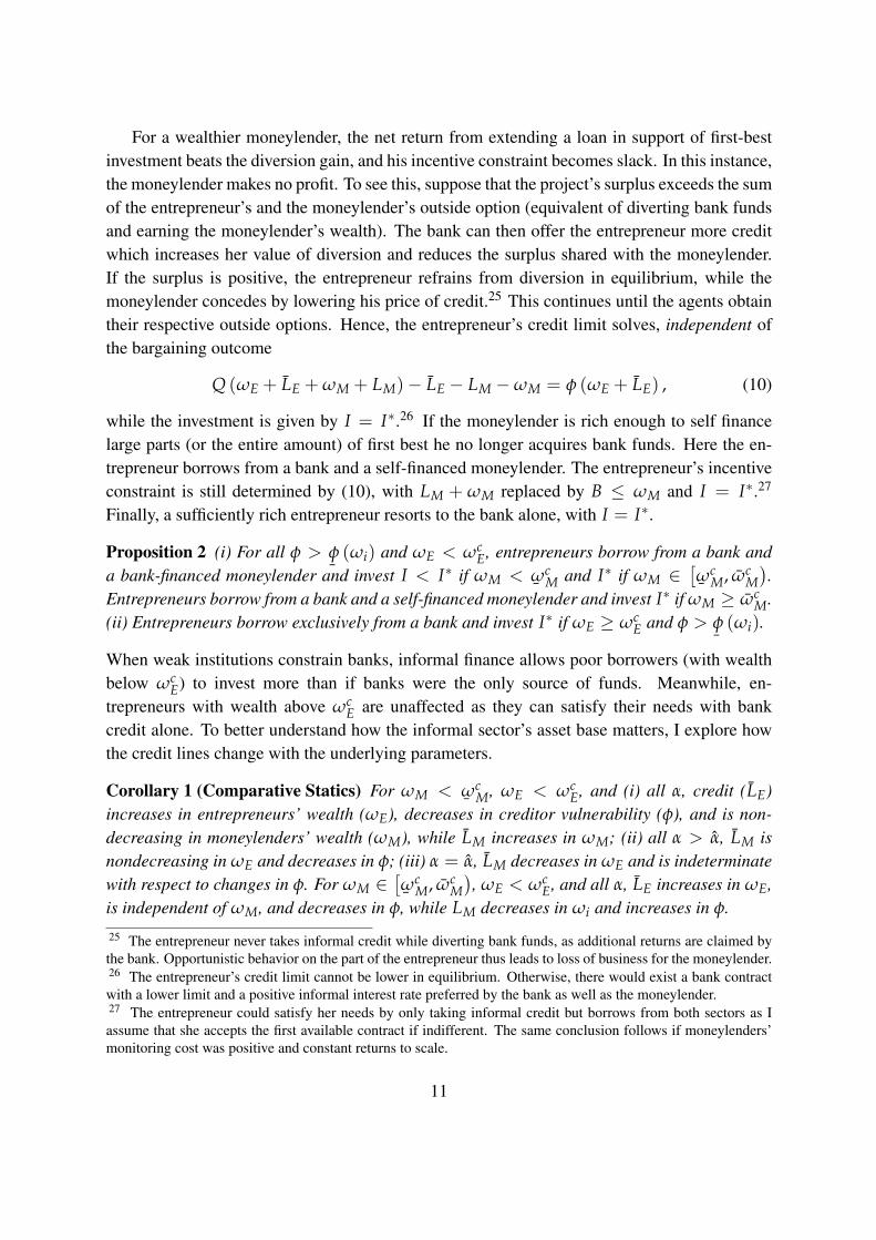
For a wealthier moneylender, the net return from extending a loan in support of first-bestinvestment beats the diversion gain, and his incentive constraint becomes slack. In this instance,the moneylender makes no profit. To see this, suppose that the project’s surplus exceeds the sumof the entrepreneur’s and the moneylender’s outside option (equivalent of diverting bank fundsand earning the moneylender’s wealth). The bank can then offer the entrepreneur more creditwhich increases her value of diversion and reduces the surplus shared with the moneylender.If the surplus is positive, the entrepreneur refrains from diversion in equilibrium, while themoneylender concedes by lowering his price of credit.25 This continues until the agents obtaintheir respective outside options. Hence, the entrepreneur’s credit limit solves, independent ofthe bargaining outcome

Q (ωE + LE + ωM + LM)− LE − LM −ωM = φ (ωE + LE) , (10)

while the investment is given by I = I∗.26 If the moneylender is rich enough to self financelarge parts (or the entire amount) of first best he no longer acquires bank funds. Here the en-trepreneur borrows from a bank and a self-financed moneylender. The entrepreneur’s incentiveconstraint is still determined by (10), with LM + ωM replaced by B ≤ ωM and I = I∗.27

Finally, a sufficiently rich entrepreneur resorts to the bank alone, with I = I∗.

Proposition 2 (i) For all φ > φ¯

(ωi) and ωE < ωcE, entrepreneurs borrow from a bank and

a bank-financed moneylender and invest I < I∗ if ωM < ω¯

cM and I∗ if ωM ∈

[ω¯

cM, ωc

M).

Entrepreneurs borrow from a bank and a self-financed moneylender and invest I∗ if ωM ≥ ωcM.

(ii) Entrepreneurs borrow exclusively from a bank and invest I∗ if ωE ≥ ωcE and φ > φ

¯(ωi).

When weak institutions constrain banks, informal finance allows poor borrowers (with wealthbelow ωc

E) to invest more than if banks were the only source of funds. Meanwhile, en-trepreneurs with wealth above ωc

E are unaffected as they can satisfy their needs with bankcredit alone. To better understand how the informal sector’s asset base matters, I explore howthe credit lines change with the underlying parameters.

Corollary 1 (Comparative Statics) For ωM < ω¯

cM, ωE < ωc

E, and (i) all α, credit (LE)increases in entrepreneurs’ wealth (ωE), decreases in creditor vulnerability (φ), and is non-decreasing in moneylenders’ wealth (ωM), while LM increases in ωM; (ii) all α > α, LM isnondecreasing in ωE and decreases in φ; (iii) α = α, LM decreases in ωE and is indeterminatewith respect to changes in φ. For ωM ∈

[ω¯

cM, ωc

M), ωE < ωc

E, and all α, LE increases in ωE,is independent of ωM, and decreases in φ, while LM decreases in ωi and increases in φ.

25 The entrepreneur never takes informal credit while diverting bank funds, as additional returns are claimed bythe bank. Opportunistic behavior on the part of the entrepreneur thus leads to loss of business for the moneylender.26 The entrepreneur’s credit limit cannot be lower in equilibrium. Otherwise, there would exist a bank contractwith a lower limit and a positive informal interest rate preferred by the bank as well as the moneylender.27 The entrepreneur could satisfy her needs by only taking informal credit but borrows from both sectors as Iassume that she accepts the first available contract if indifferent. The same conclusion follows if moneylenders’monitoring cost was positive and constant returns to scale.

11

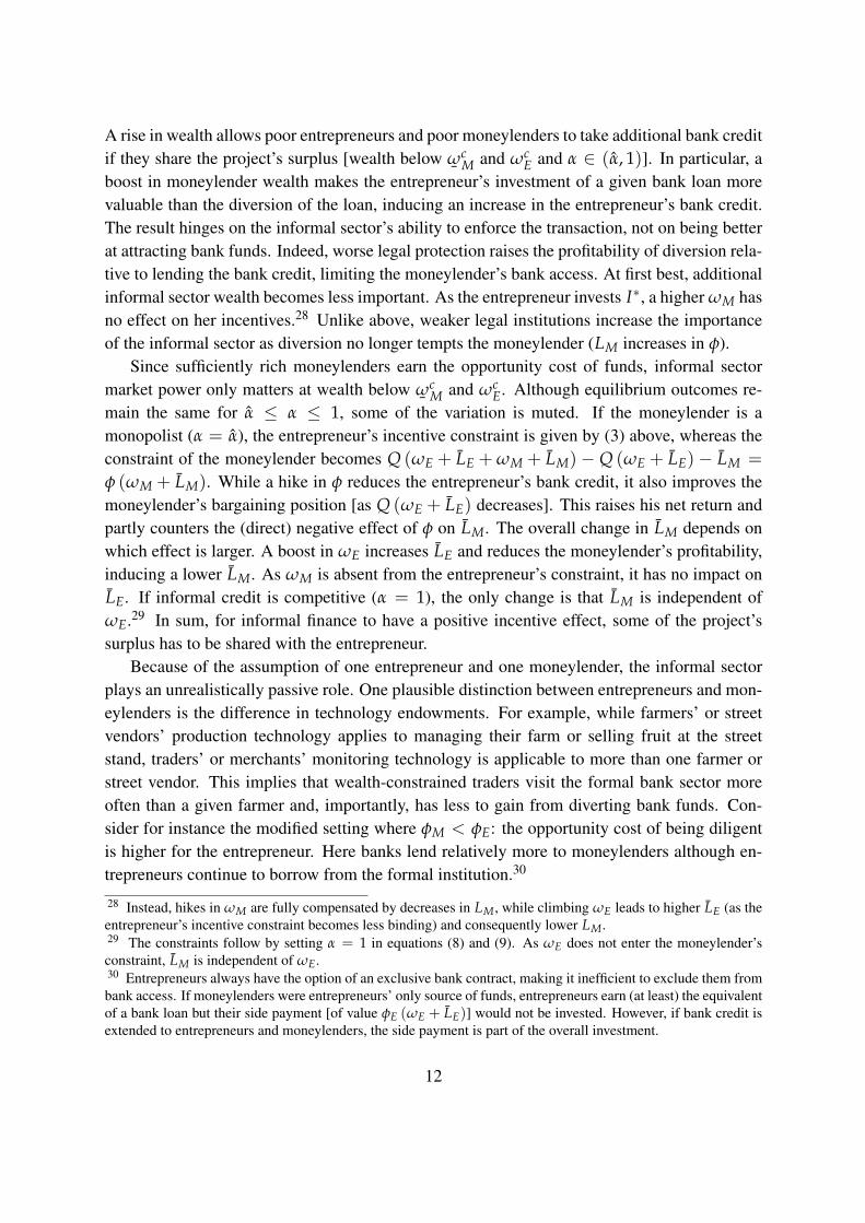
A rise in wealth allows poor entrepreneurs and poor moneylenders to take additional bank creditif they share the project’s surplus [wealth below ω

¯cM and ωc

E and α ∈ (α, 1)]. In particular, aboost in moneylender wealth makes the entrepreneur’s investment of a given bank loan morevaluable than the diversion of the loan, inducing an increase in the entrepreneur’s bank credit.The result hinges on the informal sector’s ability to enforce the transaction, not on being betterat attracting bank funds. Indeed, worse legal protection raises the profitability of diversion rela-tive to lending the bank credit, limiting the moneylender’s bank access. At first best, additionalinformal sector wealth becomes less important. As the entrepreneur invests I∗, a higher ωM hasno effect on her incentives.28 Unlike above, weaker legal institutions increase the importanceof the informal sector as diversion no longer tempts the moneylender (LM increases in φ).

Since sufficiently rich moneylenders earn the opportunity cost of funds, informal sectormarket power only matters at wealth below ω

¯cM and ωc

E. Although equilibrium outcomes re-main the same for α ≤ α ≤ 1, some of the variation is muted. If the moneylender is amonopolist (α = α), the entrepreneur’s incentive constraint is given by (3) above, whereas theconstraint of the moneylender becomes Q (ωE + LE + ωM + LM)− Q (ωE + LE)− LM =φ (ωM + LM). While a hike in φ reduces the entrepreneur’s bank credit, it also improves themoneylender’s bargaining position [as Q (ωE + LE) decreases]. This raises his net return andpartly counters the (direct) negative effect of φ on LM. The overall change in LM depends onwhich effect is larger. A boost in ωE increases LE and reduces the moneylender’s profitability,inducing a lower LM. As ωM is absent from the entrepreneur’s constraint, it has no impact onLE. If informal credit is competitive (α = 1), the only change is that LM is independent ofωE.29 In sum, for informal finance to have a positive incentive effect, some of the project’ssurplus has to be shared with the entrepreneur.

Because of the assumption of one entrepreneur and one moneylender, the informal sectorplays an unrealistically passive role. One plausible distinction between entrepreneurs and mon-eylenders is the difference in technology endowments. For example, while farmers’ or streetvendors’ production technology applies to managing their farm or selling fruit at the streetstand, traders’ or merchants’ monitoring technology is applicable to more than one farmer orstreet vendor. This implies that wealth-constrained traders visit the formal bank sector moreoften than a given farmer and, importantly, has less to gain from diverting bank funds. Con-sider for instance the modified setting where φM < φE: the opportunity cost of being diligentis higher for the entrepreneur. Here banks lend relatively more to moneylenders although en-trepreneurs continue to borrow from the formal institution.30

28 Instead, hikes in ωM are fully compensated by decreases in LM, while climbing ωE leads to higher LE (as theentrepreneur’s incentive constraint becomes less binding) and consequently lower LM.29 The constraints follow by setting α = 1 in equations (8) and (9). As ωE does not enter the moneylender’sconstraint, LM is independent of ωE.30 Entrepreneurs always have the option of an exclusive bank contract, making it inefficient to exclude them frombank access. If moneylenders were entrepreneurs’ only source of funds, entrepreneurs earn (at least) the equivalentof a bank loan but their side payment [of value φE (ωE + LE)] would not be invested. However, if bank credit isextended to entrepreneurs and moneylenders, the side payment is part of the overall investment.

12

3.3 Imperfect Bank Competition

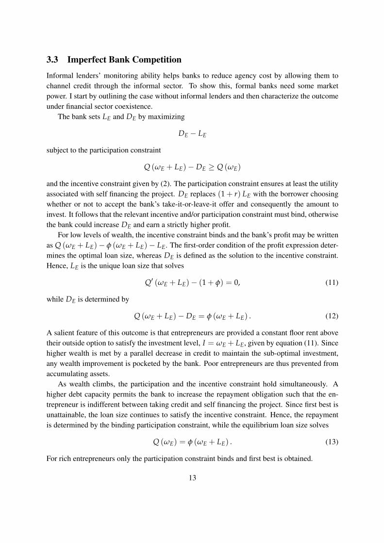
Informal lenders’ monitoring ability helps banks to reduce agency cost by allowing them tochannel credit through the informal sector. To show this, formal banks need some marketpower. I start by outlining the case without informal lenders and then characterize the outcomeunder financial sector coexistence.

The bank sets LE and DE by maximizing

DE − LE

subject to the participation constraint

Q (ωE + LE)− DE ≥ Q (ωE)

and the incentive constraint given by (2). The participation constraint ensures at least the utilityassociated with self financing the project. DE replaces (1 + r) LE with the borrower choosingwhether or not to accept the bank’s take-it-or-leave-it offer and consequently the amount toinvest. It follows that the relevant incentive and/or participation constraint must bind, otherwisethe bank could increase DE and earn a strictly higher profit.

For low levels of wealth, the incentive constraint binds and the bank’s profit may be writtenas Q (ωE + LE)− φ (ωE + LE)− LE. The first-order condition of the profit expression deter-mines the optimal loan size, whereas DE is defined as the solution to the incentive constraint.Hence, LE is the unique loan size that solves

Q′ (ωE + LE)− (1 + φ) = 0, (11)

while DE is determined by

Q (ωE + LE)− DE = φ (ωE + LE) . (12)

A salient feature of this outcome is that entrepreneurs are provided a constant floor rent abovetheir outside option to satisfy the investment level, I = ωE + LE, given by equation (11). Sincehigher wealth is met by a parallel decrease in credit to maintain the sub-optimal investment,any wealth improvement is pocketed by the bank. Poor entrepreneurs are thus prevented fromaccumulating assets.

As wealth climbs, the participation and the incentive constraint hold simultaneously. Ahigher debt capacity permits the bank to increase the repayment obligation such that the en-trepreneur is indifferent between taking credit and self financing the project. Since first best isunattainable, the loan size continues to satisfy the incentive constraint. Hence, the repaymentis determined by the binding participation constraint, while the equilibrium loan size solves

Q (ωE) = φ (ωE + LE) . (13)

For rich entrepreneurs only the participation constraint binds and first best is obtained.

13

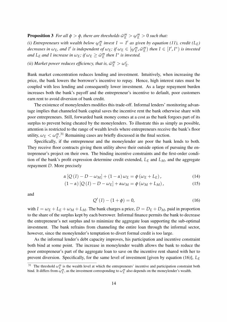
Proposition 3 For all φ > φ¯

, there are thresholds ωmE > ω

¯mE > 0 such that:

(i) Entrepreneurs with wealth below ω¯

mE invest I = I′ as given by equation (11), credit (LE)

decreases in ωE, and I′ is independent of ωE; if ωE ∈ [ω¯

mE , ωm

E ) then I ∈ [I′, I∗) is investedand LE and I increase in ωE; if ωE ≥ ωm

E then I∗ is invested.

(ii) Market power reduces efficiency, that is, ωmE > ωc

E.

Bank market concentration reduces lending and investment. Intuitively, when increasing theprice, the bank lowers the borrower’s incentive to repay. Hence, high interest rates must becoupled with less lending and consequently lower investment. As a large repayment burdenincreases both the bank’s payoff and the entrepreneur’s incentive to default, poor customersearn rent to avoid diversion of bank credit.

The existence of moneylenders modifies this trade-off. Informal lenders’ monitoring advan-tage implies that channeled bank capital saves the incentive rent the bank otherwise share withpoor entrepreneurs. Still, forwarded bank money comes at a cost as the bank forgoes part of itssurplus to prevent being cheated by the moneylenders. To illustrate this as simply as possible,attention is restricted to the range of wealth levels where entrepreneurs receive the bank’s floorutility, ωE < ωm

E .31 Remaining cases are briefly discussed in the final section.Specifically, if the entrepreneur and the moneylender are poor the bank lends to both.

They receive floor contracts giving them utility above their outside option of pursuing the en-trepreneur’s project on their own. The binding incentive constraints and the first-order condi-tion of the bank’s profit expression determine credit extended, LE and LM, and the aggregaterepayment D. More precisely

α [Q (I)− D−ωM] + (1− α) ωE = φ (ωE + LE) , (14)

(1− α) [Q (I)− D−ωE] + αωM = φ (ωM + LM) , (15)

andQ′ (I)− (1 + φ) = 0, (16)

with I = ωE + LE + ωM + LM. The bank charges a price, D = DE + DM, paid in proportionto the share of the surplus kept by each borrower. Informal finance permits the bank to decreasethe entrepreneur’s net surplus and to minimize the aggregate loan supporting the sub-optimalinvestment. The bank refrains from channeling the entire loan through the informal sector,however, since the moneylender’s temptation to divert formal credit is too large.

As the informal lender’s debt capacity improves, his participation and incentive constraintboth bind at some point. The increase in moneylender wealth allows the bank to reduce thepoor entrepreneur’s part of the aggregate loan to save on the incentive rent shared with her toprevent diversion. Specifically, for the same level of investment [given by equation (16)], LE

31 The threshold ωmE is the wealth level at which the entrepreneurs’ incentive and participation constraint both

bind. It differs from ω¯

mE , as the investment corresponding to ωm

E also depends on the moneylender’s wealth.

14

is decreased in step with a climbing ωM until the entire loan is extended to the moneylender,giving rise to credit market segmentation. The moneylender’s repayment obligation DM solvesthe binding participation constraint

(1− α) [Q (I)− DM −ωE] + αωM = (1− α) [Q (ωE + ωM)−ωE] + αωM, (17)

while the equilibrium loan size LM satisfies

(1− α) [Q (ωE + ωM)−ωE] + αωM = φ (ωM + LM) , (18)

with I = ωE + ωM + LM. The participation constraint ensures the utility associated with themoneylender self financing the project.

A rich enough moneylender is able to support first best. Equation (17) determines DM andI = I∗. Finally, if the moneylender is sufficiently wealthy to self finance the investment, thebank and the moneylender compete in the same fashion as described by equation (10) above.

Proposition 4 For all φ > φ¯

(ωi) and ωE < ωmE , entrepreneurs borrow from a bank and

a bank-financed moneylender and invest I = I′ as given by equation (16) if ωM < ω¯

mM.

Entrepreneurs borrow exclusively from a bank-financed moneylender and invest I ∈ [I′, I∗) ifωM ∈

[ω¯

mM, ωm

M)

and I∗ if ωM ∈[ωm

M, I∗ −ωE). Entrepreneurs borrow from a bank and a

self-financed moneylender and invest I∗ if ωM ≥ I∗ −ωE.

While informal finance raises bank-rationed borrowers’ investment, it also limits formal sectoraccess. As moneylenders become richer, banks are able to reduce the surplus otherwise sharedwith poor entrepreneurs. This contrasts with and complements the findings of Proposition2 and Corollary 1. In poor societies with weak legal institutions, moneylenders’ monitoringability therefore induces two opposing effects. On the one hand, informal finance complementsbanks by allowing more formal capital to reach borrowers directly. On the other hand, informallenders substitute for banks by acting as a formal credit channel. The extent to which eithereffect dominates depends on the degree of competition in the formal bank sector.

Note that Proposition 4 is independent of informal lenders’ market power. Bank profit de-creases as the informal sector becomes more competitive, by reducing moneylenders’ incentive-compatible bank loan. However, this does not affect the bank’s desire to minimize poor borrow-ers’ direct involvement. Also, while the analysis assumes that the formal sector is a monopoly,it is sufficient that the bank has enough market power to make informal lenders’ participationconstraint bind at some point. Then the bank always finds it more profitable to contract exclu-sively with the informal sector rather than dealing directly with poor borrowers.

Figure (1) summarizes Propositions 2 and 4 in terms of the moneylender’s debt capacity(assuming a bank-rationed entrepreneur). The competitive benchmark is depicted above theline, with the moneylender’s incentive constraint binding below ω

¯cM. The imperfectly com-

petitive case is illustrated underneath the line. The incentive constraint binds alone below ω¯

mM

15

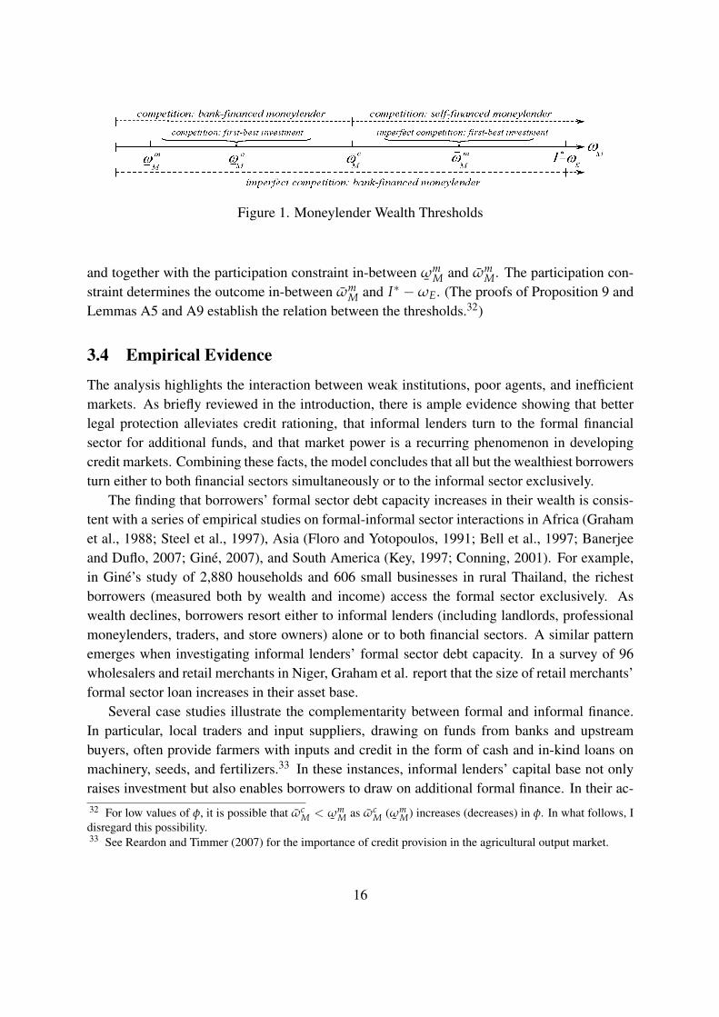
Figure 1. Moneylender Wealth Thresholds

and together with the participation constraint in-between ω¯

mM and ωm

M. The participation con-straint determines the outcome in-between ωm

M and I∗ −ωE. (The proofs of Proposition 9 andLemmas A5 and A9 establish the relation between the thresholds.32)

3.4 Empirical Evidence

The analysis highlights the interaction between weak institutions, poor agents, and inefficientmarkets. As briefly reviewed in the introduction, there is ample evidence showing that betterlegal protection alleviates credit rationing, that informal lenders turn to the formal financialsector for additional funds, and that market power is a recurring phenomenon in developingcredit markets. Combining these facts, the model concludes that all but the wealthiest borrowersturn either to both financial sectors simultaneously or to the informal sector exclusively.

The finding that borrowers’ formal sector debt capacity increases in their wealth is consis-tent with a series of empirical studies on formal-informal sector interactions in Africa (Grahamet al., 1988; Steel et al., 1997), Asia (Floro and Yotopoulos, 1991; Bell et al., 1997; Banerjeeand Duflo, 2007; Gine, 2007), and South America (Key, 1997; Conning, 2001). For example,in Gine’s study of 2,880 households and 606 small businesses in rural Thailand, the richestborrowers (measured both by wealth and income) access the formal sector exclusively. Aswealth declines, borrowers resort either to informal lenders (including landlords, professionalmoneylenders, traders, and store owners) alone or to both financial sectors. A similar patternemerges when investigating informal lenders’ formal sector debt capacity. In a survey of 96wholesalers and retail merchants in Niger, Graham et al. report that the size of retail merchants’formal sector loan increases in their asset base.

Several case studies illustrate the complementarity between formal and informal finance.In particular, local traders and input suppliers, drawing on funds from banks and upstreambuyers, often provide farmers with inputs and credit in the form of cash and in-kind loans onmachinery, seeds, and fertilizers.33 In these instances, informal lenders’ capital base not onlyraises investment but also enables borrowers to draw on additional formal finance. In their ac-32 For low values of φ, it is possible that ωc

M < ω¯

mM as ωc

M (ω¯

mM) increases (decreases) in φ. In what follows, I

disregard this possibility.33 See Reardon and Timmer (2007) for the importance of credit provision in the agricultural output market.

16

count of contract farming in North America, Latin America, and Africa, Glover and Kusterer(1990) write that the informal funding provided by traders and input suppliers “serves to as-sure banks of the farmer’s credit-worthiness, thus facilitating access to private [bank] credit”(Glover and Kusterer, 1990, p. 130).34 Related evidence is provided by Campion (2006) in herstudy of Peru’s artichoke sector. Campion documents that artichoke processors and input sup-pliers “provide valuable finance...to help farmers...to produce high quality artichokes in greaterquantity and improve their returns on investment. Higher returns have lead to greater access toformal finance...” (Campion, 2006, p. 10). Wittlinger and Tuesta’s (2006) description of soy-bean farmers in Paraguay tells a similar story. Farmers sell their produce to and receive creditfrom upstream silos that actively oversee the production process. This phase-by-phase supervi-sion means that the bank officers spend less time monitoring the loan, allowing for more formalcapital to be lent directly to the farmers. Moreover, the silos also take bank loans to financefertilizers, fuel, and agricultural equipment provided as in-kind inputs to the farmers.35

The empirical regularity that wealthier informal lenders often are the exclusive clients offormal banks (rather than poor borrowers) supports the prediction that banks may prefer tochannel their capital through the informal sector. In their study of Philippine agricultural fi-nance, Floro and Yotopoulos (1991) note that formal lenders and upstream buyers rarely dealdirectly with smaller borrowers. Instead, the formal lenders rely on rich farmer-clients as “they[the rich farmers] have the assets required for leverage” (Floro and Yotopoulos, 1991, p. 46).Similarly, Rahman (1992) reports that although formal credit totals more than two thirds ofthe informal sector’s liabilities in Bangladesh, less than ten percent of the households borrowdirectly from the formal sector. Those that take formal credit (and on lend) are “people with suf-ficient collateral and credibility to borrow from formal sector financial institutions” (Rahman,1992, p. 154). Related support is provided by Harriss (1983) in her study of 400 agriculturaltraders and paddy producers in Tamil Nandu, India where large farmers take formal credit to beon lent to poorer clients. Evidence from Japan’s Meiji era (1868-1912) shows a similar pattern.During this period, wealthier grain, fertilizer, or textile merchants, landlords, and professionalmoneylenders obtained bank credit to finance poor farmers, weavers, and silk producers other-wise unable to secure external funding (Teranishi, 2005, 2007).36

In the model, the degree of bank competition affects formal financial sector access as wellas the role of informal lenders. This is in line with historical evidence from Plymouth County inNew England, United States (Wang, 2008). Using detailed bank, census, and court records be-tween 1803 and 1850, Wang documents how increased bank competition allowed poor farmersand artisans to partially substitute from informal finance provided by wealthier (bank-financed)merchants, to formal bank credit. Bank records show that merchants, esquires, and gentle-

34 See also Watts (1994) for related support.35 For a similar account from Croatia, see Matic et al. (2006).36 See Biggs (1993) for related evidence from early twentieth century Taiwan, where larger firms on-lent com-mercial bank credit directly to smaller downstream customers lacking bank access.

17

men (the rich) accounted for most of the transactions when the county comprised one bank.37

Meanwhile, the court records of debt claims identify the same wealthy group as providers ofcredit to farmers and artisans. After the entry of an additional bank, the proportion of bankloans to merchants declined from 60 to 25 percent while farmers and artisans increased theirshare from 12 to 38 percent. The court records also show that farmers and artisans were lesslikely to borrow from wealthy merchants.38 Contemporary data echo these findings. In Gine’s(2007) study of formal-informal sector interactions in Thailand, poor borrowers are less likelyto access the informal sector exclusively when bank competition increases. Also, Burgess andPande’s (2005) investigation of the effects of bank branch expansion in India (effectively, in-creased formal sector competition) shows a similar pattern. They find that bank borrowing asa share of total rural household debt increased from 0.3 to 29 percent between 1961 and 1991.Meanwhile, borrowing from professional moneylenders fell from 61 to 16 percent in the sameperiod.39, 40

4 Cross-Sectional Predictions

This section studies one of the model’s key premises: that informal finance emerges in responseto banks’ inability to enforce their legal claims. It also investigates the implications of variationin income and in bank market structure. As the competitiveness of the informal sector, α, hasan effect on some of my findings, I initially explore results that are independent of α.

I first show that weaker institutions increase the prevalence of informal credit if borrowersobtain money from both financial sectors, while the opposite is true if moneylenders supply allfunds. Specifically, if entrepreneurs and moneylenders obtain bank credit and moneylendersare rich enough not to be tempted by diversion, the ratio of informal credit to investment,B/I = (ωM + LM) / (ωE + LE + ωM + LM), increases in creditor vulnerability φ. A hike inφ boosts the profitability of non-prudent behavior relative to investment for poor entrepreneurs,inducing a shift to agency-free informal finance (Corollary 1). Consider then the case of creditmarket segmentation. If bank-rationed moneylenders are the only providers of entrepreneurialcredit, worse legal protection causes banks to cut the funding of the informal sector to avoiddiversion. That is, the fraction B/I decreases in φ. At first best, more efficient institutions areirrelevant for B/I since diversion no longer tempts the moneylender.

My theory further predicts that the ratio B/I increases if borrowers are poor and if mon-

37 Esquires and gentlemen were honorary titles given to people with more wealth and higher social status. Es-quires could be merchants, large land-owning farmers, attorneys, and judges. Gentlemen were another economi-cally better-off class, if not quite as wealthy as esquires.38 That is, the cases where farmers appeared as defendants and merchants as plaintiffs declined after the entry.39 Note that 30 percent of the households in 1991 still held loans from the government, traders, and landlords.40 Findings from China also show that informal finance is more prevalent in the central and the northwest regionswhere bank competition is scant and less important in the coastal region where banks are more competitive (Culland Xu, 2005; Ayyagari et al., forthcoming; Cheng and Degryse, 2010).

18

eylenders are better capitalized. To see this, note that a rise in entrepreneurial wealth inducesa shift from informal to formal finance and a lower B/I if moneylenders are rich enough toattain first best in the competitive benchmark.41 Higher moneylender wealth does not affectB/I though, as hikes in ωM are compensated by decreases in LM. If the entrepreneur and themoneylender obtain bank credit under imperfect bank competition, increases in wealth lead to adecrease in credit to limit diversion. For example, a higher ωE reduces the moneylender’s shareof the aggregate loan LM and B/I drops.42 By contrast, if the moneylender is the only bankborrower, bank credit increases in ωM, boosting B relatively more than I as the entrepreneur’swealth is unaffected. At first best, the outcome is analogous to the competitive case above.

Proposition 5 For bank-rationed entrepreneurs, the ratio of informal credit to investment is:

(i) Increasing in creditor vulnerability (φ), decreasing in entrepreneurs’ wealth (ωE), and in-dependent of moneylenders’ wealth (ωM) if banks are competitive and ωM ≥ ω

¯cM.

(ii) Nonincreasing in φ for ωM ≥ ω¯

mM, decreasing in ωE for ωM < ω

¯mM and for ωM ≥ ωm

M,and nondecreasing in ωM if banks have market power and ωM < I∗ −ωE.

A limitation of Proposition 5 is that it does not apply if entrepreneurs and moneylenders arerationed by competitive banks. This is because variation in φ, ωE, and ωM affects LE and LMsimultaneously, with the impact on B/I depending on how the project gains are shared. This isalso true for some of the changes in ωE under market segmentation.43 However, by restrictingattention to competitive informal credit (α = 1) and an informal monopoly (α = α), the modelgives consistent predictions both with respect to institutional quality and with respect to wealth.

Corollary 2 For bank-rationed entrepreneurs, the ratio of informal credit to investment is:

(i) Increasing in creditor vulnerability (φ) and decreasing in entrepreneurs’ wealth (ωE) forα = α, 1 and nondecreasing in moneylenders’ wealth (ωM) for α = α if banks arecompetitive.

(ii) Nonincreasing in ωE for α = α, 1 if banks have market power and ωM < I∗ −ωE.

The results presented in Proposition 5 thus continue to hold in this restricted setting. Inter-estingly, the first part of Corollary 2 shows that informal finance becomes more important asinstitutional quality deteriorates even when informal lenders are poor. This is because the reduc-tion in entrepreneurs’ bank credit that follows from a higher φ dominates the drop in informallenders’ bank credit. To see this, consider a monopolistic moneylender under bank competi-tion. A boost in φ reduces LE, while the effect on LM is ambiguous due to the moneylender’s

41 That is, LE (LM) increases (decreases) following a boost in ωE (Corollary 1).42 As investment is locked at the suboptimal level [given by equation (16)], an increase in ωE only improves theentrepreneur’s bargaining position, forcing the bank to lower LM.43 The effect of φ on B/I is ambiguous below ω

¯mM (when entrepreneurs and moneylenders access the bank under

imperfect bank competition), as a higher φ leads to less bank lending and a lower suboptimal investment [givenby (16)]. The total effect depends on which reduction is larger (independently of how project proceeds are split).

19

improved bargaining position (Corollary 1). If informal credit is competitive, the decline in LEexceeds the fall in LM, since the entrepreneur keeps the full surplus and subsequently holds alarger part of the aggregate bank loan. (Wealth results follow in similar fashion from Corollary1.) Under market segmentation, the moneylender’s loan and the fraction B/I is independent ofentrepreneurial wealth if α = 1, as ωE does not enter equation (18). If α = α, the moneylen-der’s net return and, consequently, his bank loan and the ratio B/I decrease in ωE.

Propositions 2 and 4 indicate that the relative importance of bank-financed moneylendersincreases in banks’ market power. To show this formally, I first characterize the economy’ssupply of bank credit. As market structure is irrelevant if moneylenders rely on internal funds,attention is restricted to wealth levels where informal lenders need external capital.

Lemma 1 (i) Entrepreneurs obtain more funds from competitive banks. (ii) There exists athreshold ωM(φ) ∈

(ω¯

cM, ωc

M)

such that moneylenders with wealth below ωM obtain morefunds from competitive banks and moneylenders with wealth above ωM obtain more fundsunder imperfect bank competition.

Since all benefits accrue to the entrepreneurs under competitive banking, competitive bankssupply more credit as a result of improved incentives. Moneylenders take more competitivebank credit up to first best (ω

¯cM), then reduce their loan in step with rising wealth. Meanwhile,

the imperfectly competitive bank continues to extend additional funds as the efficient outcome(ωm

M) remains to be attained. [For details, see Figure (1).]

Proposition 6 The ratio of informal credit to investment is higher when banks have marketpower and ωM ∈ (ωM, I∗ −ωE) and indeterminate with respect to bank market structure forwealth below ωM.

While entrepreneurs obtain more funds from poor moneylenders if banks compete, they alsotake additional bank credit (Lemma 1), making the exact prediction imprecise. However, asmoneylenders become wealthier the outcome is clear: informal finance should be more impor-tant if it allows banks to save the agency costs.

Using firm-level data for 26 countries in Eastern Europe and Central Asia, Dabla-Norris andKoeda (2008) broadly confirm Proposition 5 and Corollary 2. They show that the relationshipbetween legal institutions and informal credit is indeterminate, while bank lending contracts ascreditor protection worsens. More systematic evidence is offered in a recent study by Chavis etal. (2009) covering 70,000 small and medium-sized firms in over 100 countries. As implied bythe model, improvements in creditor protection have a positive effect on access to bank finance,particularly for young (and small) firms.44 Specifically, the interaction between rule of lawand firm age is significant and negative for bank finance. Meanwhile, there is no significant

44 A drawback of these findings is their focus on firm age rather than firm size/collateral. Other variables, such asreputation, may have an independent effect on credit access besides collateral. However, to the extent that youngfirms still have lower wealth, the empirical evidence does corroborate the model’s conclusions.

20

interactive effect of rule of law for finance coming from informal sources and trade credit.My theory explains the insignificant effect by showing that the relationship can go either way,while bank credit—if accessible—increases in creditor protection. Dabla-Norris and Koedaand Chavis et al. also find that the use of informal finance is consistently higher in lower-income countries. If entrepreneurial wealth is a proxy for income, this is line with the model’sprediction that informal finance grows in importance as borrower wealth declines. Finally,Proposition 6 concurs with the findings of Burgess and Pande (2005), Gine (2007), and Wang(2008), that informal finance is more prevalent as bank markets become less competitive.

5 Welfare, Segmentation, and Financial Development

Why does financial sector underdevelopment, in the form of market segmentation, persist? Onereason is that those who potentially influence the levers of power (for example, wealthy infor-mal lenders and influential bankers) gain from status quo. I investigate this issue by consideringhow welfare is distributed in the economy.

Proposition 7 (i) Entrepreneurs and poor moneylenders, ωM < ω¯

cM, are better off when banks

are competitive, whereas banks and sufficiently wealthy moneylenders, ωM > ω¯

cM, are better

off when banks have market power. (ii) Entrepreneurs prefer a bank with market power overthe coexistence of a moneylender and a bank with market power.

Informal finance supports entrepreneurs’ asset growth in the competitive setting. The reason istwofold. Competition transfers the entire surplus to the bank borrowers, allowing more creditto be extended. Moneylenders reinforce this effect by further expanding credit provision and bysoftening the entrepreneurs’ incentive problem. Competition also adds value to poor moneylen-ders as they receive more bank funds. By contrast, banks and wealthier moneylenders are betteroff if financial markets are segmented. This is because the segmented outcome preserves themarket power that moneylenders’ enforcement advantage grants them (α remains unchanged),whereas they are forced to give up all their rent under competitive banking (α = 1). Part (ii)of Proposition 7 makes borrowers’ welfare loss explicit. Poor entrepreneurs receive less fundsand consequently lower floor utility from the monopoly bank (for a given investment) if it alsoextends credit to the moneylender. If moneylenders provide all external capital, entrepreneursearn the equivalent of doing the project alone with the informal lender, worth strictly less thanthe incentive rent provided by the bank.

Besides allowing banks to reduce agency cost, credit market segmentation also softens com-petition between the formal and the informal financial sector, providing an additional rationalefor its persistence. This resonates with the work of Rajan and Zingales (2003) on incumbentfinancial institutions’ historical support for financial repression to maintain status quo. In par-ticular, suppose rich moneylenders and bankers have more say over local bank market structurethan poor entrepreneurs, for example, through branching restrictions on banking. In this case,

21

Proposition 7 provides a political-economy explanation as to why informal finance and bankmarket power are pervasive features of less developed credit markets. In line with my the-ory, Rajan and Ramcharan (forthcoming) find that bank markets in the early twentieth centuryUnited States were more concentrated in counties with wealthy landowners, who often engagedin lending to local farmers. These landlords frequently had ties with the local bank and the localstore (that offered credit) and were, as the model predicts, against bank deregulation.45 Rajanand Ramcharan show that there were fewer banks per capita and less formal bank lending topoor farmers (as well as higher formal interest rates) in counties with a more unequal distribu-tion of farm land. This is consistent with the skewed distribution of wealth needed to support thetheory’s predictions. In the model, relatively better-off informal lenders are more creditworthycompared to poor entrepreneurs.

6 Informal Interest Rates

Aleem (1990), Banerjee (2003), and others have shown that poor borrowers with similar char-acteristics face informal interest rates ranging from 0 to 200 percent annually in India, Pakistan,and Thailand.46 In fact, there is large variation in informal lending rates even within the samesub economy. I now examine factors that may explain some of the observed heterogeneity.

Proposition 8 (i) Bank-rationed moneylenders charge positive rates of interest, R/B− 1 > 0.(ii) R/B − 1 is nondecreasing in creditor vulnerability (φ) if moneylenders keep the entiresurplus. (iii) R/B− 1 is higher when banks have market power and increases as credit marketsbecome segmented.

First, poor moneylenders charge positive rates of interest regardless of the degree of competitionin the adjacent bank market. This is because the price of informal credit reflects the incentiverent moneylenders receive to ensure prudent behavior when forwarding bank funds. Compe-tition from the bank sector is thus softened as excessive lending to poor entrepreneurs and/orpoor moneylenders would result in diversion. By contrast, a self-financed informal sector offerscredit at the opportunity cost of funds.

Second and related to the first point, weaker institutions causes interest rates to rise if bank-rationed moneylenders are monopolists.47 That is, an increase in the opportunity cost of be-ing diligent, φ, transmits into a higher price of informal credit. Specifically, the interest ratebecomes R/B − 1 = [Q (ωE + LE + ωM + LM)−Q (ωE + LE)] / (ωM + LM) − 1 when

45 In his study of farm credit in Texas, Haney (1914) writes that the “country merchant act as the banker’s agentin making crop mortgage loans” (Haney, 1914, p. 54). Haney estimates that as much as 20 percent of all loans inTexas banks were made to country merchants for the purpose of funding crop mortage securities.46 For additional evidence, see Udry (1990, 1994) and La Ferrara (2003) for the case of Africa and Das-Gupta etal. (1989) and Siamwalla et al. (1990) for the case of Asia.47 As noted in Section 4, general predictions on the effect of creditor vulnerability are difficult to make unless werestrict attention to either a competitive or a monopolistic informal credit market.

22

banks compete. Corollary 1 states that a higher φ reduces LE, while the effect on LM is am-biguous. The moneylender’s stronger bargaining position thus enables him to increase therepayment obligation R; an increase which dominates the ambiguous effect on the loan sizeB.48 Under market segmentation, an increase in φ limits bank lending to the moneylender butdoes not affect wealth, explaining why the reduction in B is larger relative to the drop in R.At first-best investment, institutional changes have no bite.49 Finally, if the cost of diversionφ differs between moneylenders (not only across legal environments), perhaps because theydiffer in the number of formal loans outstanding or in the social ties with the formal banker,this generates additional variation in the interest charged within the same sub economy.

Third, as poor moneylenders extend more credit under competitive banking this leads tolower interest rates due to diminishing returns to scale. Also, if moneylender wealth climbs,informal lenders offer credit at the opportunity cost of funds in the competitive setting. Mean-while, the segmented outcome not only preserves moneylenders’ market power, it also increasesinterest rates further as entrepreneurs lose their outside option when dealing exclusively withthe informal sector.50

Terms offered to the same borrower thus range from an effective price of zero to very highrates. Accounting for the institutional environment and the possibility of market segmentationcomplements the emphasis on monitoring cost as an explanation for the steep lending rates(see Banerjee, 2003). In my setting, the zero interest result partly depends on the assumptionof zero monitoring cost. However, while allowing for positive monitoring cost on part of themoneylender adds another layer, it does not qualitatively alter the findings.

7 Economic Policy

Before I consider possible reforms, let me summarize the main results so far.51 The model’sbasic distortion is the inability of formal banks to enforce their contracts. Better functioninginstitutions not only allow banks to lend more to poor borrowers and poor informal lenders, theycan also reduce informal interest rates.52 If the aim is to replace informal with formal finance,wealth subsidies may be more effective policy however. While the prevalence of informalfinance decreases in entrepreneurial wealth, informal credit becomes more important as legal

48 Similar intuition explains the outcome when the entrepreneur and the moneylender both obtain bank financein the imperfectly competitive case.49 R/B− 1 is insensitive to variation in φ under first best in the competitive benchmark, although entrepreneurs’credit is affected. This is because competition leads moneylenders to lend at the opportunity cost of funds.50 In effect, without the bank’s incentive rent entering the bargaining, entrepreneurs are charged the same pricethat they would have paid if no bank were present.51 In what follows, I examine policies that are productivity enhancing, that is, they raise investment. This doesnot imply Pareto efficiency however; see Bardhan et al. (2000) for a discussion.52 The interaction between creditor vulnerability and the credit market endogenously determines the threshold ofwealth necessary to attain an efficient investment using only bank funds. Hence, stronger creditor protection alsoimplies that entrepreneurs with less wealth will succeed in securing an exclusive bank contract.

23

protection of banks improves if credit markets are segmented.Propositions 2 and 4 show that financial sector coexistence increases efficiency compared

to a pure bank lending regime. The policy recommendations that follow are straightforwardfrom an efficiency perspective, but less clear in terms of borrower welfare. Although regulationfostering informal sector growth is beneficial for poor borrowers in the competitive benchmark,the opposite is true under credit market segmentation (Proposition 7). Moreover, while pro-competitive bank reforms raise efficiency,53 help borrowers access the formal sector, and reduceinformal interest rates, the caveat may be the lack of political will to introduce such policies, asdiscussed in Section 5. Hence, programs that strengthen borrowers’ outside options (similar tothe empowerment strategies of poor tenants documented in Banerjee et al., 2002) offer a way todiminish the reliance on credit provided by informal lenders and banks. Specifically, it pointsto the importance of alternative sources of credit, such as microfinance. In fact, microfinanceprograms may present a more viable alternative if powerful vested interests (in the form ofwealthy informal lenders and banks) are opposed to bank market reforms.

I now analyze the effects of subsidized credit by allowing for a positive cost of bank capital,ρ. Introducing ρ has three effects: it offers a deposit return that enters the outside option inthe bargaining, it affects the residual return for a given loan size, and it alters the sub-optimalinvestment if banks have market power. While a lower ρ increases investment if the moneylen-der and the entrepreneur obtain bank credit—regardless of bank market structure—it decreaseslending to the bank-rationed moneylender and subsequent investment under market segmenta-tion. This is because a drop in ρ weakens the moneylender’s outside option in his bargainingwith the entrepreneur, while the bank’s price is unaffected [as DM > (1 + ρ) LM]. The endeffect is a decrease in the prevalence of informal finance and lower efficiency.54

Proposition 9 (i) Financial sector coexistence and bank market competition increase invest-ment (I). (ii) I decreases in the opportunity cost of capital (ρ), except if moneylenders are bankrationed under credit market segmentation, then I increases in ρ.

Which reform is most efficient? In what follows, I explore the differential impact of changes increditor protection, cost of capital, and wealth in terms of gross benefits. Under bank compe-tition, reduced creditor vulnerability boosts investment more than a lower cost of capital. Thereason is that φ influences the marginal return to the entire investment, whereas ρ only affectsthe return to the bank loan. Specifically, a drop in φ decreases the opportunity cost of beingdiligent with bank credit (LE + LM) and with internal funds (ωE + ωM), while a reduction

53 In the proof of Proposition 9, I show that ωmM > ωc

M. That is, a moneylender stops borrowing from competitivebanks before first best is attained in the imperfectly competitive case. [See Figure (1).]54 Exogenously imposed formal interest rate ceilings have a weakly positive effect on efficiency. Under compet-itive banking, the policy never binds. (This assumes that banks are to break even. If the policy implies that banksshould exceed the endogenously determined credit limit, lending will result in diversion.) In the imperfectly com-petitive case, interest rate ceilings increase bank lending if they bind. Also, if they prohibit banks from chargingan interest rate such that moneylenders’ participation constraint binds, credit market segmentation fails to occur.

24

in ρ increases the residual return for a given loan (LE + LM). In the imperfectly competitivescenario, two cases need to be considered. When the entrepreneur and the moneylender borrowfrom the bank, changes in creditor vulnerability and cost of capital have an analogous impacton the sub-optimal investment given by equation (16).55 Under market segmentation, a lowerφ increases investment (Proposition 5), while a reduction in ρ decreases it (Proposition 9).56

Wealth subsidies to borrowers follow the standard prescription in credit-rationing models,where redistribution in favor of poor entrepreneurs supports increased borrowing and invest-ment. In my model, informal lenders also face binding credit constraints, suggesting that thesepolicy implications need to be modified. Consider a reform that redistributes one dollar from theentrepreneur to the moneylender. If rationed entrepreneurs and moneylenders access the bank,the transfer affects the bargaining weights and subsequent bank lending, but not the project’ssize since every dollar is invested. Under market segmentation, a reallocation in favor of thebank-rationed moneylender increases investment. As the moneylender’s share of the invest-ment, not the overall size, determines the incentive-compatible bank loan [equation (18)], anadditional dollar of moneylender wealth draws more bank money into the project.57 A similarresult is obtained in the competitive benchmark if entrepreneurs’ opportunity cost of being dili-gent exceeds moneylenders’ cost, φM < φE. Although every dollar is invested, moneylendersattract more bank credit since they are less likely to divert the funds. In sum, while grants topoor entrepreneurs increase investment and decrease the prevalence of informal finance, trans-fers to the informal sector may be a more efficient policy choice.

Proposition 10 Investment (I) increases weakly if: (i) Creditor vulnerability (φ) decreasesrather than the opportunity cost of capital (ρ) and I < I∗. (ii) Wealth is redistributed fromentrepreneurs to moneylenders.

Redistribution raises investment partly because of moneylenders’ perfect monitoring ability.If entrepreneurs invest a fraction of the informal loan, the statement remains correct undercredit market segmentation, while the policy lowers efficiency in the competitive benchmark.Inefficient monitoring matters less under segmentation as the transfer’s main effect in this casecomes through a shift in the relative bargaining weights. However, if the diversion return ishigher for the entrepreneurs, φM < φE, the proposition is still valid, given that the informalmonitoring technology is efficient enough and/or the difference φE − φM is sufficiently large.

8 Discussion and Concluding Remarks

A worthwhile question is why the bank does not merge with the moneylender, making him thelocal branch manager? Specifically, the bank supplies the financial resources and the moneylen-55 More specifically, the modified equation reads Q′ (I)− (1 + φ + ρ) = 0.56 At first best, variation in φ has no effect on investment while a reduction in ρ increases investment by changingthe optimal project size, determined by Q′ (I)− (1 + ρ) = 0.57 At first-best investment, marginal wealth reallocation no longer matters.

25

der the local knowledge. In the current setting, internal funds are a necessary condition however.Incentive compatibility is violated if banks extend credit to penniless informal lenders/bank em-ployees. Consider the competitive benchmark and a perfectly competitive informal sector. Inthis case, moneylenders’ incentive constraint collapses to R− LM = LM − LM = 0 < φLM.But it is also true when moneylenders hold all the bargaining power.58 Two important obser-vations follow. First, it is not sufficient to have a superior enforcement technology to on lendbank funds. Second, informal lenders are not bank agents; they need to put their own moneyat stake to facilitate the intermediation of formal credit. In sum, “bringing the market insidethe firm” at best replicates the market outcome, as the branch manager has to be incentivizedto act responsibly with the bank funds. However, the merger also adds a new dimension, theemployer-employee relationship, which opens up for opportunistic behavior on the part of thebank as well.59, 60 Hence, the overall effect is likely to be efficiency reducing, confirming whythis kind of organizational design is uncommon in developing credit markets.61

A related concern is whether the key insights would be altered if informal monitoring wasless efficient, if other sharing rules governed the moneylender’s and the entrepreneur’s ex-change, or if agents engaged in side payments? As regards the first objection, suppose theentrepreneur fails to invest a fraction δ ∈ (0, 1) of the moneylender’s funds.62 It can be shownthat for δ sufficiently small, equilibrium outcomes remain the same. Pertaining to the choiceof sharing rule, the Nash Bargaining solution produces an efficient outcome similar to Coasianbargaining since utility is transferable. Any sharing rule therefore yields quantitatively similarresults in terms of the ensuing investment. Finally, side payments do not change the equilib-rium outcomes since poor entrepreneurs and/or poor moneylenders are unable to compensatethe other party and/or the bank due to their wealth constraints. That is, available funds arealways used most efficiently in production.

Allowing for rising entrepreneurial wealth in the imperfectly competitive case changes lit-tle if the entrepreneur’s wealth climbs and wealth disparity is maintained. Here the bank isindifferent between dealing with the (relatively) richer moneylender alone and lending a smallamount to the entrepreneur and the remainder to the moneylender. If the entrepreneur is the

58 First, note that the project’s aggregate incentive-compatible bank loan is the same, with or without the pennilessmoneylender, as he does not add to investment. Second, when α = α, the entrepreneur receives her outside option,equivalent of exclusive bank borrowing, but this is exactly the value of the entire project including the moneylender.Hence, after compensating the entrepreneur, the moneylender earns zero. When bank competition is imperfect, aloan to a penniless moneylender satisfies incentive compatibility. However, entrepreneurs prefer an exclusive bankcontract as it increases their incentive rent. Since the bank is indifferent between lending to entrepreneurs alone orboth (aggregate rent and loan size remain the same) and entrepreneurs are the project’s proprietors, moneylendersget shut out.59 Similar in spirit to Williamson’s (1985) arguments of why “selective interventions” are hard to implement.60 Moreover, if there is output uncertainty and monitoring cost is positive, bank managers may be tempted toreduce monitoring and subsequent monitoring cost only to claim that entrepreneurial failure was due to exogenousevents. (Allowing for output uncertainty would not change the theory’s main predictions.)61 See Varghese (2004) for a survey of the issue.62 The value δ could be a deadweight loss or, alternatively, a benefit accruing directly to the entrepreneur.

26

richer party, the outcome resembles the one analyzed in detail above, now with the bank gradu-ally reducing its loan to the poor moneylender. If entrepreneurs and moneylenders are equallyaffluent though short of first best, both receive credit. Finally, similar to bank competition, richentrepreneurs only take bank credit. Thus what matters for the results is that informal lendershold relatively more assets compared to entrepreneurs.

As the model stands, informal lenders’ occupational choice is restricted to lending. Thesetup has allowed me to analyze how the basic traits uniting informal lenders: local enforce-ment and some wealth, shape less developed credit markets. In a more general setting, ad-ditional sources of income (and/or collateral) make it less tempting to behave non diligently,enabling the bank to extend more funds or save on incentive-related costs. Extending the the-ory by admitting complementary sources of income would permit for a characterization of howinformal lenders’ enforcement technology and debt capacity vary across occupation and howmonitoring ability and wealth interact in attracting outside funding. For example, are inputsuppliers better suited to extend credit to poor farmers and draw on external capital, as com-pared to landlords, merchants, shopkeepers, and upstream buyers? It would also be interestingto explore the question of who becomes a moneylender. Such a model has the potential toexplain, among other things, how the informal sector’s market power is determined. If enforce-ment rests on social sanctions available within a community but all members are equally poor,anyone can become a moneylender, as well as attract outside funding. By contrast, if one vil-lager is slightly wealthier than the rest, she will attract all outside funding and become the localmonopolist. Another topic for future research would be to develop a more explicit political-economy model to understand the interaction between the credit market and the formation ofinterest groups.

In closing, the theory laid out in this paper lends itself to empirical testing. While the keyfindings stand up well to the available evidence, more quantitative work is needed to thoroughlyunderstand how the informal sector’s resource constraints affect its ability to finance poor bor-rowers as well as attract outside funding. Combining systematic data on informal lenders’ debtcapacity with measures of institutional quality and market structure would also allow for fur-ther tests of the model’s predictions. Detailed micro evidence that sheds light on the role playedby informal finance would be an important complement to the growing experimental literatureinvestigating credit markets in developing countries.

27

AppendixThe following result will be helpful in the subsequent analysis.

Lemma A2 Q′ (ωE + LE)− (1 + φ) < 0.

Proof. When the entrepreneur (henceforth E) borrows from a competitive bank (henceforthB) and the credit limit binds,

Q (ωE + LE)− LE − φ (ωE + LE) = 0. (A1)

This constraint is only binding if Q′ (ωE + LE) − (1 + φ) < 0. Otherwise, LE could beincreased without violating the constraint.

Proof of Proposition 1Proposition 1 is proved in the main text, except for the comparative static results and the exis-tence and the uniqueness of ωc

E.

Lemma A3 There exists a unique threshold ωcE (φ) > 0 such that Q (ωE + LE) − LE −

φ (ωE + LE) = 0 for ωE = ωcE (φ) and ωE + LE = I∗.

Proof. The threshold ωcE is the smallest wealth level that satisfies ωE + LE = I∗. As (A1)

yields the maximum incentive-compatible investment level, ωcE satisfies

Q (I∗)− I∗ (1 + φ) + ωcE = 0. (A2)

The threshold is unique if LE is increasing in ωE. Differentiating (A1) with respect to LE andωE I obtain

dLE

dωE=

φ−Q′ (ωE + LE)Q′ (ωE + LE)− (1 + φ)

> 0,

where the inequality follows from Lemma A2, Q′ (I) ≥ 1, and φ < 1. Finally, ωcE > 0 is a

result of the assumption that φ > φ¯

[equation (1)].

Lemma A4 If ωE ≤ ωcE then LE and I increase in ωE and decrease in φ.

Proof. The proof that dLE/dωE > 0 is provided in Lemma A3. As (A1) also determinesthe investment level, dI/dωE > 0 follows. Differentiating (A1) with respect to LE and φ Iobtain

dLE

dφ=

ωE + LE

Q′ (ωE + LE)− (1 + φ)< 0,

where the inequality follows from Lemma A2. As (A1) also determines the investment level,dI/dφ < 0 follows.

Proof of Proposition 2I show the existence and the uniqueness of ωc

E, ω¯

cM, and ωc

M and proceed with the equilibriumoutcomes.

28

Lemma A5 There exist unique thresholds ωcE(φ) > 0, ω

¯cM(φ), and ωc

M(φ) such that:(i) Q (ωE + LE)− LE − φ (ωE + LE) = 0 for ωE = ωc

E (φ) and ωE + LE = I∗;

(ii) α [Q (ωE + LE + ωM + LM)− LE − LM −ωM] + (1− α) ωE − φ (ωE + LE) = 0 and(1− α) [Q (ωE + LE + ωM + LM)− LE − LM −ωE] + αωM − φ (ωM + LM) = 0 for ωM= ω

¯cM (φ) and ωE + LE + ωM + LM = I∗;

(iii) Q (ωE + LE + ωM)− LE−ωM− φ (ωE + LE) = 0 for ωM = ωcM (φ) and ωE + LE +

ωM = I∗; and

(iv) ωcM(φ) > ω

¯cM(φ) > 0.

Proof. Part (i): The proof is provided in Lemma A3.Part (ii): The threshold ω

¯cM is the smallest wealth level that satisfies ωE + LE + ωM +

LM = I∗ when E and the moneylender (henceforth M) utilize bank funds as given by (8)and (9) in the main text. Using (8) and (9) to solve for the maximum incentive-compatibleinvestment level I have that, for a given level of E’s wealth, ωE, ω

¯cM satisfies

Q (I∗)− I∗ (1 + φ) + ωE + ω¯

cM = 0. (A3)

The threshold is unique if both LE and LM are increasing in ωM. Differentiating (8) and (9)with respect to LE, LM and ωM using Cramer’s rule I obtain

dLE

dωM=

α [Q′ (I)− 1]φ [1 + φ−Q′ (I)]

> 0

anddLM

dωM=

φ [Q′ (I)− φ]− α [Q′ (I)− 1]φ [1 + φ−Q′ (I)]

> 0,

where the inequalities follow from Lemma A2, Q′ (I) ≥ 1, and φ < 1.Part (iii): The threshold ωc

M is the smallest wealth level that satisfies ωE + LE + ωM = I∗

at which M is able to self finance E. Thus, for a given level of E’s wealth, ωE, ωcM satisfies

Q(I∗)− I∗ (1 + φ) + ωE + ωcMφ = 0. (A4)

The threshold is unique if LE (LM) is independent of (decreasing in) ωM when the relevantconstraints are given by (10) in the main text and the first-order condition Q′ (I)− 1 = 0. Dif-ferentiating (10) and the first-order condition with respect to LE, LM, and ωM using Cramer’srule I obtain

dLE

dωM= 0

anddLM

dωM= −1.

Part (iv): Combining (A3) and (A4), yields ω¯

cM = φωc

M, where ωcM > ω

¯cM follows from

φ < 1. Finally, ω¯

cM > 0 is a result of the assumption that φ > φ

¯(ωE) [equation (4)].

29

Lemma A6 If (i) ωE < ωcE and ωM < ωc

M then the entrepreneur borrows from a bank anda bank-financed moneylender. If (ii) ωE < ωc

E and ωM ≥ ωcM then the entrepreneur borrows

from a bank and a self-financed moneylender. If (iii) ωE ≥ ωcE then the entrepreneur borrows

exclusively from a bank.

Proof. I consider E’s and M’s incentive constraints given that B breaks even. Five distinctcases need to be analyzed as E may borrow from: (i) B exclusively; (ii) B and a bank-financedM; (iii) a bank-financed M exclusively; (iv) a self-financed M exclusively; (v) B and a self-financed M.

Part (i): First, consider ωM < ω¯

cM. Recognizing the concavity of Q (I) and Q′ (I) ≥ 1, it

follows that E and M prefer Case (ii) to Cases (iii)-(v) for any α. Finally, for α > α as defined inthe main text, E prefers Case (ii) to Case (i) as well. Next, when ωM ∈

[ω¯

cM, ωc

M), ωE + ωM

accounts for the interval of credit lines such that ωM < I∗−ωE− LE, for a given ωE and ωM.From the main text we have that Case (ii) leaves E with the full surplus, while M is indifferentand so Case (ii) remains the equilibrium outcome when ωM ∈

[ω¯

cM, ωc

M).

Part (ii): Here, ωE + ωM accounts for the interval of credit lines such that ωM ≥ I∗ −ωE − LE, for a given ωE and ωM. The only difference from Part (ii) is that M refrains frombank borrowing when he is able to self finance large parts of the first-best investment, makingCase (ii) irrelevant. Thus, Case (v) is the only possible outcome since in Cases (iii) and (iv), Ewould have to share part of a (possibly smaller) surplus with M.

Part (iii): As E turns to B first and is able to satisfy first best, Case (i) is the outcome.

Proof of Corollary 1 (Comparative Statics)Proof. For ωM < ω

¯cM and ωE < ωc

E: Differentiating (8) and (9) in the main text withrespect to LE, LM, ωE, ωM, and φ using Cramer’s rule I obtain (for α ∈ (α, 1])

dLE

dωE=

φ [Q′ (I)− φ]− (1− α) [Q′ (I)− 1]φ [1 + φ−Q′ (I)]

> 0,

dLM

dωE=

(1− α) [Q′ (I)− 1]φ [1 + φ−Q′ (I)]

≥ 0,

dLE

dφ=

(ωE + LE) (1− α) [Q′ (I)− 1]− φ − (ωM + LM) α [Q′ (I)− 1]φ [1 + φ−Q′ (I)]

< 0,

and

dLM

dφ=

(ωM + LM) α [Q′ (I)− 1]− φ − (ωE + LE) (1− α) [Q′ (I)− 1]φ [1 + φ−Q′ (I)]

< 0,

where the inequalities follow from Lemma A2, Q′ (I) ≥ 1, and φ < 1. The proof thatdLE/dωM ≥ 0 and dLM/dωM > 0 is provided in Lemma A5. If α = α, the relevantconstraints are given by (3) in the main text and by

Q (ωE + LE + ωM + LM)−Q (ωE + LE)− LM = φ (ωM + LM) . (A5)

30

Differentiating (3) and (A5) with respect to LE, LM, ωE, ωM, and φ using Cramer’s rule Iobtain

dLE

dωE=

φ−Q′ (ωE + LE)Q′ (ωE + LE)− (1 + φ)

> 0,

dLM

dωE=

Q′ (I)−Q′ (ωE + LE)[Q′ (ωE + LE)− (1 + φ)] [Q′ (I)− (1 + φ)]

< 0,

dLE

dωM= 0,

dLM

dωM=

φ−Q′ (I)Q′ (I)− (1 + φ)

> 0,

dLE

dφ=

ωE + LE

Q′ (ωE + LE)− (1 + φ)< 0,

and

dLM

dφ=

(ωM + LM) [Q′ (ωE + LE)− (1 + φ)]− (ωE + LE) [Q′ (I)−Q′ (ωE + LE)][Q′ (ωE + LE)− (1 + φ)] [Q′ (I)− (1 + φ)]

≶0,

where the inequalities and the indeterminacy follow from Lemma A2, Q′ (I) ≥ 1, and φ < 1.For ωM ∈

[ω¯

cM, ωc

M), ωE < ωc

E, and all α: The relevant constraints are given by (10)in the main text and the first-order condition Q′ (I) − 1 = 0. Differentiating (10) and thefirst-order condition with respect to LE, LM, ωE, ωM, and φ using Cramer’s rule I obtain

dLE

dωE=

1− φ

φ> 0,

dLM

dωE=−1φ

< 0,

dLE

dφ=− (ωE + LE)

φ< 0,

anddLM

dφ=

ωE + LE

φ> 0,

where the first inequality follows from φ < 1. The proof that dLE/dωM = 0 and dLM/dωM <0 is provided in Lemma A5.

Proof of Proposition 3Proposition 3 is proved in the main text, except for the comparative static results and the exis-tence and the uniqueness of ω

¯mE and ωm

E .

Lemma A7 There exist unique thresholds ω¯

mE (φ) and ωm

E (φ) such that:(i) φ (ωE + LE)−Q (ωE) = 0 for ωE = ω

¯mE (φ) and ωE + LE = I, with the investment level

given by equation (11) in the main text;

31

(ii) φ (ωE + LE)−Q (ωE) = 0 for ωE = ωmE (φ) and ωE + LE = I∗; and

(iii) ωmE (φ) > ω

¯mE (φ) > 0 and ωm

E (φ) > ωcE (φ).

Proof. Part (i): The threshold ω¯

mE is the smallest wealth level at which E’s incentive con-

straint equals her participation constraint allowing E to invest ωE + LE = I, with I given by(11) in the main text. Thus, ω

¯mE satisfies

φI −Q(ω¯

mE ) = 0. (A6)

The threshold is unique if LE is decreasing in ωE when the equilibrium is given by (11) and(12) in the main text. Differentiating (11) and (12) with respect to LE and ωE using Cramer’srule I obtain

dLE

dωE= −1.

Finally, ω¯

mE > 0 follows from the assumption that φ > φ

¯.

Part (ii): The proof is analogous to the proof of Part (ii) and omitted.Part (iii): Solving for ω

¯mE and ωm

E and combining the two expressions, yields Q (ωmE ) I′ =

Q (ω¯

mE ) I∗, with I′ given by (11) in the main text. By concavity, I∗ > I′ and hence ωm

E > ω¯

mE .

Solving for ωcE and ωm

E and combining the two expressions, yields Q (I∗)− I∗ = Q (ωmE )−

ωcE, where ωm

E > ωcE follows from concavity.

Lemma A8 If ωE ≤ ω¯

mE then LE decreases in ωE and I is independent of ωE; if ωE ∈

(ω¯

mE , ωm

E ) then LE and I increase in ωE.

Proof. When ωE ≤ ω¯

mE , the proof that dLE/dωE < 0 is provided in Lemma A7. Differen-

tiating (11) and (12) in the main text and the investment condition, ωE + LE = I, with respectto I and ωE using Cramer’s rule I obtain

dIdωE

= 0.

When ωE ∈ (ω¯

mE , ωm

E ), the relevant constraints are given by (13) in the main text, the bindingparticipation constraint, Q (ωE + LE)− DE = Q (ωE), and the investment condition, ωE +LE = I. Differentiating (13), the binding participation constraint, and the investment conditionwith respect to LE, I, and ωE using Cramer’s rule I obtain

dLE

dωE=

Q′ (ωE)− φ

φ> 0

anddI

dωE=

Q′ (ωE)φ

> 0,

where the first inequality follows from Q′ (I) ≥ 1 and φ < 1.

Proof of Proposition 4I show the existence and the uniqueness of ωm

E , ω¯

mM, and ωm

M and proceed with the equilibriumoutcomes.

32

Lemma A9 There exist unique thresholds ωmE (φ) > 0, ω

¯mM (φ), and ωm

M (φ) such that:(i) φ (ωE + LE)− αQ (ωE + B)− (1− α) ωE + αB = 0 for ωE = ωm

E (φ) and ωE + LE +B = I, with the investment level given by equation (16) in the main text;

(ii) φ (ωM + LM)− (1− α) [Q (ωE + ωM)−ωE]− αωM = 0 for ωM = ω¯

mM (φ) and ωE +

ωM + LM = I, with the investment level given by equation (16) in the main text;

(iii) φ (ωM + LM) − (1 − α) [Q (ωE + ωM)−ωE] − αωM = 0 for ωM = ωmM (φ) and

ωE + ωM + LM = I∗; and

(iv) ωmM(φ) > ω

¯mM(φ) > 0.

Proof. Part (i): The threshold ωmE is the smallest wealth level at which E’s incentive con-

straint equals her participation constraint allowing E to invest ωE + LE + B = I, with I givenby (16) in the main text. Thus, for a given level of M’s wealth, ωM, ωm

E satisfies

φ (I − B)− αQ (ωmE + ωM)− (1− α) ωm

E + αωM = 0. (A7)

The threshold is unique if LE + LM decrease in ωE when the equilibrium is given by (14) to (16)in the main text. The same reasoning applies when ωM ∈ [ω

¯mM, I∗ − ωE). Differentiating

(14) to (16) with respect to LE, LM, and ωE using Cramer’s rule I obtain

dLE

dωE=

1− α− φ

φ

anddLM

dωE=

α− 1φ

,

with dLE/dωE + dLM/dωE = −1. To show ωmE > 0, let α = α in (A7). This yields

φ (I − B) − Q (ωmE ) = 0, where ωm

E > 0 follows from the assumption that φ > φ¯. Then

let α = 1. Here, φ (I − B)− Q (ωmE + ωM) + ωM = 0. Note that ωm

E decreases in ωM forωM < I∗ − ωE. As ωM approaches I∗−ωE, I have that φ (I∗−ωM)−Q (I∗) +I∗−ωm

E =0,which is identical to (A4). If ωm

E =0 then ωM=I∗, but this contradicts ωcM<I∗. Hence, ωm

E >0.Part (ii): The threshold ω

¯mM is the smallest wealth level at which M’s incentive constraint

equals his participation constraint allowing an investment of ωE + ωM + LM = I, with I givenby (16) in the main text. Thus, for a given level of E’s wealth, ωE, ω

¯mM satisfies

φ (I −ωE)− (1− α) [Q(ωE + ω¯

mM)−ωE]− αω

¯mM = 0. (A8)

The threshold is unique if LE + LM decrease in ωM when the equilibrium is given by (14)to (16) in the main text. Differentiating (14) to (16) with respect to LE, LM, and ωM usingCramer’s rule I obtain

dLE

dωM=−α

φ

anddLM

dωM=

α− φ

φ,

33

with dLE/dωM + dLM/dωM = −1.Part (iii): The threshold ωm

M is the smallest wealth level at which M’s incentive constraintequals his participation constraint allowing an investment of ωE + ωM + LM = I∗. Thus, fora given level of E’s wealth, ωE, ωm

M satisfies

φ (I∗ −ωE)− (1− α) [Q(ωE + ωmM)−ωE]− αωm

M = 0. (A9)

The threshold is unique if LM is increasing in ωM when the equilibrium is given by (17) and(18) in the main text. Differentiating (17) and (18) with respect to LM and ωM using Cramer’srule I obtain

dLM

dωM=

(1− α) Q′ (ωE + ωM) + α− φ

φ> 0,

where the inequality follows from Q′ (I) ≥ 1 and φ < 1.Part (iv): Combining (A8) and (A9), yields (I′ −ωE) (1− α) [Q(ωE + ωm

M) − ωE] +αωm

M = (I∗ −ωE) (1− α) [Q(ωE + ω¯

mM) − ωE] + αω

¯mM, with I′ given by (16) in the

main text, and hence ωmM>ω

¯mM. Finally, ω

¯mM>0 follows from the assumption that φ>φ

¯.

Lemma A10 If (i) ωE < ωmE and ωM < ω

¯mM then the entrepreneur borrows from a bank and a

bank-financed moneylender. If (ii) ωE < ωmE and ωM ∈

[ω¯

mM, I∗ −ωE

)then the entrepreneur

borrows exclusively from a bank-financed moneylender. If (iii) ωE < ωmE and ωM ≥ I∗ −ωE

then the entrepreneur borrows from a bank and a self-financed moneylender.

Proof. I consider B’s utility given that the relevant (incentive or participation) constraint ofE and M is satisfied.

Part (i): There are two distinct cases to consider when ωE < ωmE and ωM < ω

¯mM. First,

if the incentive constraints of E and M bind, B prefers lending to both rather than only one ofthem as this minimizes the aggregate loan size needed to satisfy I′ [given by (16) in the maintext]. When M’s participation and incentive constraint hold simultaneously, B can either: (i)scale up the loan to E and M, allowing the investment to rise above I′; or (ii) maintain I = I′

by reallocating the loan from E to M in response to an increase in M’s wealth. Suppose Case(i) is a candidate equilibrium, as defined by (14) to (16) in the main text. An increase in ωMallows B to increase LM to the point at which M’s incentive constraint equals his participationconstraint. M’s additional loan raises E’s investment return and permits a larger loan to E aswell. Hence, an increase in M’s wealth increases B’s utility by (differentiating UB = Q (I)−(1− α) [Q (ωE + ωM)−ωE]− αωM − φ (ωE + LE)− LE − LM with respect to ωM)

dUB

dωM=

Q′(ωE + ωM) [Q′ (I)− (1 + φ)] + φ

φ,

where Q′ (I) < 1 + φ as I > I′. Meanwhile, Case (ii) implies that an increase in ωM is metby an increase in LM and a subsequent decrease in LE satisfying dLM/dωM + dωM/dωM =−dLE/dωM. Differentiating B’s utility with respect to ωM in this case yields

dUB

dωM= 1 >

Q′(ωE + ωM) [Q′ (I)− (1 + φ)] + φ

φ.

34

Hence, when ωE < ωmE and ωM < ω

¯mM, E borrows from B and a bank-financed M with

ωE + LE + ωM + LM = I′.Part (ii): When ωE < ωm

E and ωM ∈[ω¯

mM, I∗ −ωE

)the only difference from Part (i) is

that M’s debt capacity has improved, allowing B to extend the entire loan to M as this saves theincentive rent otherwise shared with E.

Part (iii): When ωE < ωmE and ωM ≥ I∗ − ωE, M is able to self finance first-best invest-

ment and the same outcome as described in Part (ii), Lemma A6 is obtained.

Proof of Proposition 5Proof. Differentiating the ratio of informal credit to investment, B/I, with respect to φ, ωE,

and ωM yields rφ=[(dLM/dφ)I − (dI/dφ)B]/I2, rωE=[(dLM/dωE)I − (dI/dωE)B]/I2,and rωM = [d (ωM + LM) /dωM]I − (dI/dωM)B/I2, respectively. Investment is unaf-fected by variation in φ, ωE, and ωM (ωE and ωM) at first best (when it is given by (16) in themain text).

Part (i): When ωE<ωcE and ωM≥ω

¯cM, rφ= (dLM/dφ) /I>0, rωE= (dLM/dωE) /I<0,

and rωM= (1+dLM/dωM)/I=0, using the comparative statics established in Corollary 1.Part (ii): First, I derive the relevant comparative statics. When ωE < ωm

E and ωM ∈[ω¯

mM, ωm

M), the constraints are given by (17) and (18) in the main text. Differentiating (17)

and (18) with respect to LM, I, and φ using Cramer’s rule I obtain dLM/dφ = dI/dφ =−B/φ < 0. When ωE < ωm

E and ωM ∈[ωm

M, I∗ −ωE), the constraints are given by (17) in

the main text and the first-order condition Q′ (I)− 1 = 0. Differentiating (17) and the first-order condition with respect to LM, ωE, and ωM using Cramer’s rule I obtain dLM/dωE =dLM/dωM = −1. Next, I determine the ratios. When ωE < ωm

E and ωM < ω¯

mM, then

rωE = (dLM/dωE) /I < 0 and rωM = (1 + dLM/dωM) /I > 0, using the comparative stat-ics established in Lemma A9. If ωE < ωm

E and ωM ∈[ω¯

mM, ωm

M), then rφ = −BωE/φI2 < 0

and rωM = [(1− α) Q′ (ωE + ωM) + α] ωE/φI2 > 0, using the comparative statics estab-lished above and in Lemma A9. If ωE < ωm

E and ωM ∈[ωm

M, I∗ −ωE), then rφ = rωM = 0

and rωE = −1/I < 0, using the comparative statics established above.

Proof of Corollary 2Proof. Part (i): When ωE < ωc

E, ωM < ω¯

cM, and α = α the relevant constraints are

given by (3) in the main text and (A5). Differentiating (3) and (A5) with respect to I, ωE, ωM,and φ using Cramer’s rule I obtain dI/dωE = dI/dωM = [1 + φ− Q′ (ωE + LE)]/Ψ anddI/dφ = I [Q′ (ωE + LE)− (1 + φ)] /Ψ, with Ψ = [Q′ (ωE + LE)− (1 + φ)] ×[Q′ (I)− (1 + φ)] > 0, where the inequality follows from Lemma A2, Q′ (I) ≥ 1, and φ < 1.Using Corollary 1 and the derived comparative statics, I have that rφ = [B(Q′(ωE + LE)−(1 + φ)) − (ωE + LE)(Q′(I) − Q′(ωE + LE))]I − BQ′(ωE + LE) − (1 + φ))I/ΨI2 =(ωE + LE) [Q′ (ωE + LE) − Q′ (I)]/ΨI > 0, rωE = [Q′ (I) − Q′ (ωE + LE)]I −[1 + φ−Q′ (ωE + LE)]B/ΨI2 < 0, and rωM = [(Q′ (ωE + LE)− (1 + φ))(φ−Q′ (I))+ ((Q′ (ωE + LE) − (1 + φ))(Q′ (I) − (1 + φ))]I − [1 + φ − Q′ (ωE + LE)]B/ΨI2 =(ωE + LE) [1 + φ − Q′ (ωE + LE)]/ΨI2 > 0, where the inequalities follow from LemmaA2 and concavity. If α = 1, the relevant constraints are given by (8) and (9) in the maintext. Differentiating (8) and (9) with respect to I, ωE, and φ using Cramer’s rule I obtain

35

dI/dφ = −φI/Θ and dI/dωE = φ/Θ, with Θ = φ[1 + φ − Q′ (I))] > 0, where theinequality follows from Lemma A2. Using Corollary 1 and the derived comparative statics,I have that rφ = [B (Q′ (I)− (1 + φ))]I + BφI/ΘI2 = B[Q′ (I) − 1]/ΘI > 0 andrωE = −φB/ΘI2 < 0, where the inequalities follow from Q′ (I) ≥ 1. When ωE < ωc

Eand ωM ≥ ω

¯cM, the results are found in the proof of Proposition 5, Part (i).

Part (ii): When ωE < ωmE , ωM ∈

[ω¯

mM, ωm

M), and α = α the relevant constraints are given

by (17) in the main text and by

Q (ωE + ωM)−Q (ωE) = φ (ωM + LM) . (A10)

Differentiating (17) and (A10) with respect to I, LM, and ωE using Cramer’s rule I obtaindI/dωE = [φ + Q′ (ωE + ωM) − Q′ (ωE)]/φ and dLM/dωE = [Q′ (ωE + ωM) −Q′ (ωE)]/φ. Using the derived comparative statics, I have that rωE = [Q′ (ωE + ωM) −Q′ (ωE)]I − [φ + Q′ (ωE + ωM)−Q′ (ωE)]B/(−φ)I2=[Q′ (ωE + ωM)−Q′ (ωE)]ωE− φB/φI2 < 0, where the inequality follows from concavity. If α = 1, the relevant con-straints are given by (17) and (18) in the main text. Differentiating (8) and (9) with respectto I, LM, and ωE using Cramer’s rule I obtain dI/dωE = 1 and dLM/dωE = 0. Using thederived comparative statics I have that rωE = −B < 0. When ωE < ωm

E and ωM < ω¯

mM or

ωM ≥ ωmM, the results are found in the proof of Proposition 5, Part (ii).

Proof of Lemma 1[As above, the competitive (monopoly) outcome is denoted by superscript c (m).]Proof. Part (i): There are two distinct cases to consider. First, when ωM < ω

¯mM, Ic > Im

follows from Lemma A2, (16) in the main text, and concavity. Combining (8) and (9) and(14) and (15) in the main text, yields Q (Ic) − Ic = φIc and Q (Im) − D = φIm, respec-tively. Subtracting Lm

E from LcE using E’s incentive constraints given by (8) and (14) yields

α[Q (Ic) − Ic − (Q (Im)− D)] = α (Ic − Im) > 0 and hence LcE > Lm

E . Next, whenωM ∈

[ω¯

mM, I∗−ωE

), monopoly bank lending to E ceases, hence Lc

E > LmE = 0.

Part (ii): I begin by showing the existence and the uniqueness of ωM. From Lemma A5,dLc

M/dωM < 0 when ωM ∈(ω¯

cM, ωc

M). In addition, from Lemma A9, dLm

M/dωM > 0when ωM ∈

(ω¯

mM, ωm

M). By continuity and Proposition 9, there exists a unique threshold

ωM = ωM(φ) for ωM ∈(ω¯

cM, ωc

M)

at which LcM = Lm

M. Having established the existenceand the uniqueness of ωM, there are four distinct cases to consider. First, when ωM < ω

¯mM, the

proof is analogous to the proof of Part (i) resulting in LcM > Lm

M. Second, suppose LmM > Lc

Mwhen ωM ∈

[ω¯

mM, ωM

). This implies that ωm

M < ω¯

cM, which contradicts Proposition 9 and so

LcM > Lm

M. Third, when ωM ∈[ωM, ωc

M)

I have from Lemma A10 that LmM ≥ Lc

M. Fourth,when ωM ∈

[ωc

M, I∗ −ωE), competitive bank lending to M ceases, hence Lm

M > LcM = 0.

Proof of Proposition 6Proof. When ωM ∈ (ωM, I∗−ωE), Bm/Im−Bc/Ic = (Bm Ic−Bc Im) /Im Ic > 0, since

Bm > Bc from Lemma 1 and Ic ≥ Im. When ωM < ωM, Bm/Im − Bc/Ic is indeterminate,as Bm < Bc from Lemma 1, while Ic > Im.

Proof of Proposition 7(Let Ui

E and UiM denote E’s and M’s respective utility.)

36

Proof. Part (i): First, from Lemma 1 I have that LcE > Lm

E . Hence, for ωM < ω¯

mM, Uc

E =φ (ωE + Lc

E) > φ (ωE + LmE ) = Um

E and for ωM ∈[ω¯

mM, I∗ −ωE

), Uc

E = φ (ωE + LcE) >

φ (ωE + LmE ) > αQ (ωE + ωM) + (1− α) ωE − αωM = Um

E . Next, when ωM < ω¯

cM,

UcM = φ

(ωM + Lc

M)

> φ(ωM + Lm

M)

= UmM. When ωM ∈

[ω¯

cM, I∗ −ωE

), Uc

M = ωM <(1− α) (Q(ωE + ωM)−ωE) + αωM = Um

M.Part (ii): Denote isolation by Umi

E and coexistence by UmcE . For ωM < ω

¯mM, Umi

E = φI′ >φ (I′ −ωM − LM) = Umc

E [with I′ given by (16) in the main text] and for ωM∈[ω¯

mM, I∗−ωE

),

UmiE = φI′ > φ (I′ −ωM − LM) > αQ (ωE + ωM) + (1− α) ωE − αωM = Umc

E .

Proof of Proposition 8Proof. Part (i): It suffices to show that Rc/Bc − 1 > 0 for ωM < ω

¯cM, as Rm/Bm >

Rc/Bc (established in Part (iii) below). Hence, from (9) in the main text, I have that Rc/Bc −1 = [φ(ωM + Lc

M)−ωM]/(ωM + LcM) > 0, where the inequality follows from ωM < ω

¯cM.

Part (ii): Differentiating the informal interest rate, R/B−1, with respect to φ yields i=[(dR/dφ)B−(dB/dφ)R]/B2. In the competitive benchmark, when ωE< ωc

E, ωM<ω¯

cM, and

α=α, the relevant constraints are given by (3) in the main text and (A5). Differentiating (3) and(A5) with respect to I and φ using Cramer’s rule I obtain dI/dφ=I[Q′(ωE+LE)−(1+φ)]/Ω,with Ω = [Q′ (ωE + LE)− (1 + φ)] [Q′ (I)− (1 + φ)] > 0, where the inequality followsfrom Lemma A2. Using Corollary 1 and the derived comparative static, I have that i =B[IQ′ (I) (Q′ (ωE + LE) − (1 + φ)) − (ωE + LE)Q′ (ωE + LE) (Q′(I) − (1 + φ))] −R[B(Q′(ωE+LE)−(1 + φ))−(ωE+LE)(Q′(ωE+LE)−Q′(I)]/ΩB2. Note that R|α=α =Q(ωE+LE+B)−Q(ωE+LE). Applying the mean-value theorem yields R = BQ′(ξ), whereQ′(ξ)∈(Q′(I), Q′(ωE+LE)). Inserting into i and simplifying, I have that i= B[Q′(ωE+LE)− (1 + φ)][Q′ (I)−Q′ (ξ)] + (ωE + LE)[Q′ (ωE + LE)−Q′ (I)][1 + φ−Q′ (ξ)]/ΩB >0, where the inequality follows from Lemma A2 and concavity. At first best, variation in φ nolonger affects R/B− 1. In the monopoly case, when ωE < ωm

E , ωM < ω¯

mM, and α = α, the

relevant constraints are given by

Q (ωE + βL)− DE = φ (ωE + βL) , (A11)Q (I)−Q (ωE + βL)− DM = φ (ωM + (1− β) L) , (A12)

andQ′ (I)− (1 + φ) = 0, (A13)

with I = ωE + ωM + L, where LE = βL, LM = (1− β) L, and β ∈ (0, 1). Differentiating (3)and (A5) with respect to I, L, and φ using Cramer’s rule I obtain dI/dφ = dL/dφ = 1/Q

′′(I).

Using the derived comparative statics and noting that R = Q (I)− Q (ωE + βL), I have thati = B[Q′ (I)− βQ′ (ωE + βL)]− (1− β)[Q (I)− Q (ωE + βL)]/Q

′′(I) B2. Applying

the mean-value theorem and simplifying, I have that i = [Q′ (I) − βQ′ (ωE + βL) − (1−β)Q′ (ϑ)]/Q

′′(I) B > 0, with Q′ (ϑ) ∈ (Q′ (I) , Q′ (ωE + βL)), where the inequality fol-

lows from concavity. When ωE < ωmE , ωM ∈

[ω¯

mM, ωm

M), and α = α the relevant constraints

are given by (17) in the main text and by (A10). Differentiating (17) and (A10) with respectto I, LM, and φ using Cramer’s rule I obtain dI/dφ = dLM/dφ = −(ωM + LM)/φ. Us-ing the derived comparative static and noting that R = Q (I) − Q (ωE), I have that i =

37

BQ′ (I)− [Q (I)−Q (ωE)]/(−φ)B. Applying the mean-value theorem and simplifying, Ihave that i = [Q′ (δ)−Q′ (I)]/φ > 0, with Q′ (δ) ∈ (Q′ (I) , Q′ (ωE)), where the inequalityfollows from concavity. At first best, variation in φ no longer affects R/B− 1.

Part (iii): I first demonstrate that Rm/Bm > Rc/Bc and then show that Rm/Bm increasesunder credit market segmentation. First, when ωM < ω

¯mM, let α = 1. This gives Rm/Bm −

Rc/Bc=(RmBc − RcBm)/BmBc=(

DM + ωM −ωM − LmM

)/Bm=

(DM − Lm

M)

/Bm ≥ 0.Then let α=α. This gives Bc[Q (Im)−Q (ωE+Lm

E )]−Bm[Q (Ic)−Q (ωE+LcE)]/BmBc.

Applying the mean-value theorem yields BmBc[Q′ (ε) − Q′ (δ)]/BmBc, where Q′ (ε) ∈(Q′ (Im) , Q′ (ωE + Lm

E )) and Q′ (δ) ∈ (Q′ (Ic) , Q′ (ωE + LcE)). From Lemma A2 and (16)

in the main text, I have that Q′ (Im) > Q′ (ωE + LcE) and hence Rm/Bm > Rc/Bc. Next,

when ωM ∈[ω¯

mM, ω

¯cM

)and proceeding in analogous fashion by taking limits, I have again

that Rm/Bm > Rc/Bc. Finally, when ωM ∈[ω¯

cM, I∗ −ωE

), Rc/Bc = 1 and the claim

follows trivially.I now determine how Rm/Bm changes as result of segmentation. To do this, I evaluate

Rm/Bm at ωM = ω¯

mM and compare with Rm/Bm at ωM = ω

¯mM − ε. Here, LE = δ, LM =

LM(ω¯

mM

)−γ, where ε, δ, and γ are small, strictly positive, and satisfy δ=ε+γ, as investment

is constant. First, let α=1. This gives Rm/Bm−Rm/Bm=Bm [φI + ε−Q (ωE+ωM)] +DE − δ [Q (I)−Q (ωE+ωM) + ωM]/BmBm, with φI = φ (ωE + δ) + φ (ωM + LM) =φ (ωE + δ) + ωM > Q (ωE + ωM) − ωM + ωM = Q (ωE + ωM), where the inequalityfollows from ωE < ωm

E . Hence, for δ sufficiently small, Rm/Bm > Rm/Bm. Next, let α = α.This gives Bm [Q(I)−Q(ωE + δ)]− δ [Q (I)−Q (ωE)]/BmBm. Again, for δ sufficientlysmall, Rm/Bm > Rm/Bm.

Proof of Proposition 9Proof. Part (i): I start with financial sector coexistence. Under competitive banking, the

relevant constraints are given by (A2) and (A3). Denote the critical ωE that satisfies (A3) byωc

E. Comparison yields ωcE > ωc

E > 0, where the last inequality follows from the assumptionthat φ > φ

¯(ωM). Under monopoly banking, two investment levels I′ [given by (16) in the

main text] and I∗ need to be verified. Starting with I′ and combining (A6) and (A7), yieldsQ(ω

¯mE ) = αQ (ωm

E + B) + (1− α) ωmE − αB + φB. As the critical threshold ωm

E decreasesin α, it follows from concavity that ω

¯mE > ωm

E . The proof when I = I∗ is analogous andomitted. Next, I turn to bank market power. First, note that ωm

M as defined by (A9) decreasesin ωE. In particular, allow ωE to increase up to the point at which φ (ωE + LE)− αQ(ωE +ωM) − (1− α) ωE + αωM = 0 for ωE + LE + ωM = I∗, or φ (I∗ −ωM) − αQ(ωE +ωM)− (1− α) ωE + αωM = 0. Denote the critical ωM that satisfies this last equality by ωm

M.From the previous argument it follows that ωm

M < ωmM. Hence, to show that ωc

M < ωmM, it

suffices to verify that ωcM < ωm

M. Then, observe that ωmM decreases in α. Hence, combining the

expression for ωmM as defined above with the expression for ωc

M as given by (A4) and allowingα = 1, yields I∗[Q(I∗)− I∗ − Q(ωE + ωm

M) + ωE + ωmM] + ωc

M[Q(ωE + ωm

M)− ωmM

]−

ωmM[Q(I∗) − I∗ + ωE] = 0. Let [Q(I∗) − I∗ − Q(ωE + ωm

M) + ωE + ωmM] ≡ Φ, where

Φ > 0 by concavity and Q′ (I) ≥ 1. Suppose first that ωmM = ωc

M. This implies that(I∗ − ωm

M)

Φ = 0. But this equality contradicts I∗ > ωmM and Φ > 0. Suppose then that

38

ωmM = ωc

M + ε. This yields(

I∗ − ωmM

)Φ + ε

[Q(ωE + ωm

M)− ωmM

]= 0, which again

generates a contradiction since Q(ωE + ωmM) > ωm

M. It follows that ωcM < ωm

M, establishingthe claim.

Part (ii): Opportunity cost of capital, ρ, enters as a multiplicative term with respect tothe credit lines, (1 + ρ) Li, and the wealth, (1 + ρ) ωi, in the competitive benchmark. WhenωE < ωc

E and ωM < ω¯

cM, the relevant constraints are given by (8) and (9) in the main

text. Differentiating (8) and (9) with respect to I and ρ using Cramer’s rule I obtain dI/dρ =−φ (LE + LM) / (1 + ρ + φ−Q′(I)) < 0, where the inequality follows from Lemma A2.When ωE < ωc

E and ωM > ω¯

cM, investment is determined by the first-order condition

Q′ (I) − (1 + ρ) = 0, with dI/dρ = 1/Q′′(I) < 0, where the inequality follows from

concavity. Under monopoly, investment is determined by (16) in the main text when ωE < ωmE

and ωM < ω¯

mM. The modified equation reads, Q′(I) − (1 + ρ + φ) = 0, with dI/dρ =

1/Q′′(I) < 0, where the inequality follows from concavity. When ωE < ωm

E and ωM ∈[ω¯

mM, ωm

M)

the relevant constraints are given by (17) and (18) in the main text. Here, ρ onlyaffects the return on the outside option, (1 + ρ) ωi. Differentiating (17) and (18) with respectto I and ρ using Cramer’s rule I obtain dI/dρ = [αωM − (1− α) ωE] /φ. The derivativeis positive if α > α∗ = ωE/ (ωE + ωM). As α ∈ (α, 1), it suffices to show that α ≥ α∗.Here, α = [Q(ωE)−ωE] / [Q(ωE + ωM)− (ωE + ωM)]. Subtracting α∗ from α yields[Q(ωE) (ωE + ωM)−Q(ωE + ωM)ωE] /[Q(ωE + ωM)− (ωE + ωM)] (ωE + ωM) >0, where the inequality follows from concavity. When ωE < ωm

E and ωM ≥ ωmM, investment

is determined by the first-order condition Q′ (I)− (1 + ρ) = 0, with dI/dρ = 1/Q′′(I) < 0,

where the inequality follows from concavity.

Proof of Proposition 10Proof. Part (i): When ωE < ωc

E and ωM < ω¯

cM in the competitive benchmark, the

relevant constraints are given by (8) and (9) in the main text. Differentiating (8) and (9) withrespect to I and φ using Cramer’s rule I obtain dI/dφ = −φI/ [1 + ρ + φ−Q′(I)] < 0,where the inequality follows from Lemma A2 (ρ is included to enable a comparison). Fromthe proof of Proposition 9 I have that dI/dρ = −φ (LE + LM) / [1 + ρ + φ−Q′(I)] and so|dI/dφ| > |dI/dρ|. Under monopoly, investment is determined by (16) in the main text whenωE < ωm

E and ωM < ω¯

mM. The modified equation reads, Q′(I) − (1 + ρ + φ) = 0, with

dI/dφ = dI/dρ = 1/Q′′(I) < 0. When ωE < ωm

E and ωM ∈[ω¯

mM, ωm

M), I have from the

proof of Proposition 5 (9) that dI/dφ < 0 (dI/dφ > 0) and the conclusion follows.Part (ii): When ωE < ωc

E and ωM < ω¯

cM in the competitive benchmark, the relevant

constraints are given by (8) and (9) in the main text. Differentiating (8) and (9) with respectto I, ωE, and ωM setting dωM = −dωE using Cramer’s rule I obtain dI/dωM = 0. Atfirst best, variation in ωE and ωM has no effect on investment. Under monopoly, investment isdetermined by (16) in the main text when ωE < ωm

E and ωM < ω¯

mM, with dI/dωi = 0. When

ωE < ωmE and ωM ∈

[ω¯

mM, ωm

M), the relevant constraints are given by (17) and (18) in the

main text. Differentiating (17) and (18) with respect to I, ωE, and ωM setting dωM = −dωEusing Cramer’s rule I obtain dI/dωM = (1− φ) /φ > 0, where the inequality follows fromφ < 1. At first best, variation in ωE and ωM has no effect on investment.

39

ReferencesAdams, Dale W., Douglas H. Graham and J.D. von Pischke. 1984. Undermining Rural Development

With Cheap Credit. Boulder: Westview Press.

Aleem, Irfan. 1990. “Imperfect Information, Screening, and the Costs of Informal Lending: A Study ofa Rural Credit Market in Pakistan.” World Bank Economic Review 4(3):329–349.

Anderson, Siwan, Jean-Marie Baland and Karl Ove Moene. 2009. “Enforcement in Informal SavingsGroups.” Journal of Development Economics 90(1):14–23.

Ayyagari, Meghana, Asli Demirguc-Kunt and Vojislav Maksimovic. forthcoming. “Formal versus Infor-mal Finance: Evidence from China.” Review of Financial Studies .

Banerjee, Abhijit V. 2003. Contracting Constraints, Credit Markets, and Economic Development. In Ad-vances in Economics and Econometrics: Theory and Applications, Eighth World Congress, VolumeIII, ed. Mathias Dewatripont, Lars Peter Hansen and Stephen Turnovsky. Cambridge UniversityPress pp. 1–46.

Banerjee, Abhijit V. and Andrew F. Newman. 1998. “Information, the Dual Economy, and Develop-ment.” Review of Economic Studies 65(4):631–653.

Banerjee, Abhijit V. and Esther Duflo. 2007. “The Economic Lives of the Poor.” Journal of EconomicPerspectives 21(1):141–167.

Banerjee, Abhijit V., Paul J. Gertler and Maitreesh Ghatak. 2002. “Empowerment and Efficiency: Ten-ancy Reform in West Bengal.” Journal of Political Economy 110(2):239–280.

Banerjee, Abhijit V., Timothy Besley and Timothy Guinnane. 1994. “Thy Neighbor’s Keeper: The De-sign of a Credit Cooperative with Theory and a Test.” Quarterly Journal of Economics 109(2):491–515.

Bardhan, Pranab, Samuel Bowles and Herbert Gintis. 2000. Wealth Inequality, Wealth Constraints andEconomic Performance. In Handbook of Income Distribution, ed. Anthony Barnes Atkinson andFrancois Bourguignon. Vol. 1 North Holland pp. 541–603.

Barth, James R., Gerard Caprio Jr. and Ross Levine. 2004. “Bank Regulation and Supervision: WhatWorks Best?” Journal of Financial Intermediation 13(2):205–248.

Beck, Thorsten, Asli Demirguc-Kunt and Vojislav Maksimovic. 2004. “Bank Competition and Accessto Finance: International Evidence.” Journal of Money, Credit, and Banking 36(3):627–648.

Bell, Clive. 1990. “Interactions Between Institutional and Informal Credit Agencies in Rural India.”World Bank Economic Review 4(3):297–327.

Bell, Clive, T.N. Srinivasan and Christopher Udry. 1997. “Rationing, Spillover and Interlinking in CreditMarkets: The Case of Rural Punjab.” Oxford Economic Papers 49:557–585.

Berensmann, Kathrin, Karl Bartels, Heike Hoffler, Kathrein Holscher, Karen Losse and Johannes Ma-jewski. 2002. Informal Financing of Small-Scale Enterprises in Sri Lanka. Reports and WorkingPapers 10/2002 German Development Institute.

Besley, Timothy and Maitreesh Ghatak. 2009. The de Soto Effect. mimeo London School of Economics.

Besley, Timothy and Stephen Coate. 1995. “Group Lending, Repayment Incentives and Social Collat-eral.” Journal of Development Economics 46:1–18.

40

Besley, Timothy, Stephen Coate and Glenn Loury. 1993. “The Economics of Rotating Savings andCredit Associations.” American Economic Review 83(4):792–810.

Besley, Timothy, Stephen Coate and Glenn Loury. 1994. “Rotating Savings and Credit Associations,Credit Markets and Efficiency.” Review of Economic Studies 61(4):701–719.

Bhaduri, Amit. 1977. “On the Formation of Usurious Interest Rates in Backward Agriculture.” Cam-bridge Journal of Economics 1(4):341–352.

Biais, Bruno and Thomas Mariotti. 2009. “Credit, Wages, and Bankruptcy Laws.” Journal of the Euro-pean Economic Association 7(5):939–973.

Biggs, Tyler S. 1993. Heterogenous Firms and Efficient Financial Intermediation in Taiwan. In Marketsin Developing Countries: Parallel, Fragmented, and Black, ed. Michael Roemer and ChristineJones. San Francisco: ICS Press pp. 167–197.

Bouman, Frits J. A. and R. Houtman. 1988. “Pawnbroking as an Instrument of Rural Banking in theThird World.” Economic Development and Cultural Change 37(1):69–89.

Braverman, Avishay and Joseph E. Stiglitz. 1982. “Sharecropping and the Interlinkage of AgrarianMarkets.” American Economic Review 72(4):695–715.

Burgess, Robin and Rohini Pande. 2005. “Do Rural Banks Matter? Evidence From the Indian SocialBanking Experiment.” American Economic Review 95(3):780–795.

Burkart, Mike and Tore Ellingsen. 2002. In-Kind Finance. Working Paper No. 3536 Centre for Economicand Policy Research.

Burkart, Mike and Tore Ellingsen. 2004. “In-Kind Finance: A Theory of Trade Credit.” AmericanEconomic Review 94(3):569–590.

Campion, Anita. 2006. Financing Artichokes and Citrus: A Study of Value Chain Finance in Peru.Microreport no 73 USAID.

Chavis, Larry W., Leora F. Klapper and Inessa Love. 2009. Entrepreneurial Finance around the World:The Impact of the Business Environment on Financing Constraints. mimeo University of NorthCarolina at Chapel Hill.

Cheng, Xiaoqiang and Hans Degryse. 2010. “The Impact of Bank and Non-Bank Financial Institutionson Local Economic Growth in China.” Journal of Financial Service Research 27(2-3):179–199.

Conning, Jonathan. 2001. Mixing and Matching Loans: Credit Rationing and Spillover in a Rural CreditMarket in Chile. mimeo Williams College.

Conning, Jonathan and Christopher Udry. 2007. Rural Financial Markets in Developing Countries. InHandbook of Agricultural Economics, Volume 3, Agricultural Development: Farmers, Farm Pro-duction, and Farm Markets, ed. Robert E. Evenson and Prabhu Pingali. North Holland pp. 2857–2910.

Cull, Robert and Lixin Colin Xu. 2005. “Institutions, Ownership, and Finance: The Determinants ofProfit Reinvestment Among Chinese Firms.” Journal of Financial Economics 77(1):117–146.

Dabla-Norris, Era and Junko Koeda. 2008. Informality and Bank Credit: Evidence from Firm-LevelData. IMF Working Papers WP/08/94 IMF.

Das-Gupta, A., C.P.S. Nayar and Associates. 1989. Urban Informal Credit Markets in India. New Delhi:National Institute of Public Finance and Policy.

41

Djankov, Simeon, Caralee McLiesh and Andrei Shleifer. 2007. “Private Credit in 129 Countries.” Jour-nal of Financial Economics 84(2):299–329.

Floro, Maria Sagrario and Debraj Ray. 1997. “Vertical Links Between Formal and Informal FinancialInstitutions.” Review of Development Economics 1(1):34–56.

Floro, Sagrario L. and Pan A. Yotopoulos. 1991. Informal Credit Markets and the New InstitutionalEconomics: The Case of Philippine Agriculture. Boulder: Westview Press.

Gates, Paul W. 1977. The Farmer’s Age: Agriculture 1815-1860. New York: Sharpe.

Germidis, Dimitri, Denis Kessler and Rachel Meghir. 1991. Financial Systems and Development: WhatRole for the Formal and Informal Financial Sectors? Paris: OECD.

Ghatak, Maitreesh and Timothy W. Guinnane. 1999. “The Economics of Lending with Joint Liability:Theory and Practice.” Journal of Development Economics 60(1):195–228.

Ghate, Prabhu, Arindam Das-Gupta, Mario Lamberte, Nipon Poapongsakorn, Dibyo Prabowo, Atiq Rah-man and T.N. Srinivasan. 1992. Informal Finance. Some Findings From Asia. Manila, Philippines:Oxford University Press.

Gine, Xavier. 2007. Access to Capital in Rural Thailand: An Estimated Model of Formal vs. InformalCredit. Research Working Paper WPS 3502 World Bank.

Glover, David and Ken Kusterer. 1990. Small Farmers, Big Business: Contract Farming and RuralDevelopment. London: Macmillan.

Graham, Douglas H., Nelson Aguilera, Michel Keita and Kifle Negash. 1988. Informal Finance in RuralNiger: Scope, Magnitudes, and Organization. Studies in Rural Finance, Economics, and SociologyOccasional Paper No. 1472 Ohio State University.

Haney, Lewis H. 1914. “Farm Credit Conditions in a Cotton State.” American Economic Review 4(1):47–67.

Harriss, Barbara. 1983. Money and Commodities: Their Interaction in a Rural Indian Setting. In RuralFinancial Markets in Developing Countries, ed. J. D. Von Pischke, Dale W. Adams and GordonDonald. Baltimore: John Hopkins University Press.

Hoff, Karla and Joseph E. Stiglitz. 1998. “Moneylenders and Bankers: Price-Increasing Subsidies in aMonopolistically Competitive Market.” Journal of Development Economics 55(2):485–518.

Holmstrom, Bengt and Jean Tirole. 1997. “Financial Intermediation, Loanable Funds, and the RealSector.” Quarterly Journal of Economics 112(3):663–691.

Irfan, M., G.M. Arif, Syed Mubashir Ali and Hina Nazli. 1999. The Structure of Informal Credit Marketin Pakistan. Research Report No. 168 Pakistan Institute of Development Economics.

Jain, Sanjay. 1999. “Symbiosis vs. Crowding-Out: The Interaction of Formal and Informal Credit Mar-kets in Developing Countries.” Journal of Development Economics 59(2):419–444.

Jain, Sanjay and Ghazala Mansuri. 2003. “A Little at a Time: The Use of Regularly Scheduled Repay-ments in Microfinance Programs.” Journal of Development Economics 72(1):253–279.

Karlan, Dean S. 2005. “Using Experimental Economics to Measure Social Capital and Predict FinancialDecisions.” American Economic Review 95(5):1688–1699.

Karlan, Dean S. 2007. “Social Connections and Group Banking.” Economic Journal 117(2):F52–F84.

42

Kranton, Rachel and Anand V. Swamy. 2008. “Contracts, Hold-Up, and Exports: Textiles and Opium inColonial India.” American Economic Review 98(3):967–989.

Kranton, Rachel E. 1996. “Reciprocal Exchange: A Self-Sustaining System.” American EconomicReview 86(4):830–851.

La Ferrara, Eliana. 2003. “Kin Groups and Reciprocity: A Model of Credit Transactions in Ghana.”American Economic Review 93(5):1730–1751.

La Porta, Rafael, Florencio Lopez de Silanes and Andrei Shleifer. 2002. “Government Ownership ofBanks.” Journal of Finance 57(1):265–301.

La Porta, Rafael, Florencio Lopez de Silanes, Andrei Shleifer and Robert W. Vishny. 1997. “LegalDeterminants of External Finance.” Journal of Finance 52:1131–1150.

La Porta, Rafael, Florencio Lopez de Silanes, Andrei Shleifer and Robert W. Vishny. 1998. “Law andFinance.” Journal of Political Economy 106(6):1113–1155.

Mansuri, Ghazala. 2006. “Credit Layering in Informal Financial Markets.” Journal of DevelopmentEconomics 84(2):715–730.

Matic, Jasna, Nanda Kozul and Zoran Cvitic. 2006. Using Value Chain Relationships to Leverage BankLending: Lessons from Croatia. Micronote USAID.

Mookherjee, Dilip and Debraj Ray. 2002. “Contractual Structure and Wealth Accumulation.” AmericanEconomic Review 92(4):818–849.

Nigel, Key. 1997. Modeling and Estimating Agricultural Household Behavior under Imperfect Markets.Ph.D. Thesis University of California, Berkeley.

Nissanke, Machiko K. and Ernest Aryeetey. 1998. Financial Integration and Development. Liberaliza-tion and Reform in sub-Saharan Africa. London: Routledge.

Petersen, Mitchell A. and Raghuram R. Rajan. 1995. “The Effect of Credit Market Competition onLending Relationships.” Quarterly Journal of Economics 110(2):407–443.

Pistor, Katarina, Martin Raiser and Stanislaw Gelfer. 2000. “Law and Finance in Transition Economies.”The Economics of Transition 8:325–368.

Rahman, Atiq. 1992. “The Informal Financial Sector in Bangladesh: An Appraisal of its Role in Devel-opment.” Development and Change 23:147–168.

Rai, Ashok S. and Tomas Sjostrom. 2004. “Is Grameen Lending Efficient? Repayment Incentives andInsurance in Village Economies.” Review of Economic Studies 71(1):217–234.

Rajan, Raghuram G. 2009. “Rent Preservation and the Persistence of Underdevelopment.” AmericanEconomic Journal: Macroeconomics 1(1):178–218.

Rajan, Raghuram G. and Luigi Zingales. 2003. Saving Capitalism from the Capitalists: Unleashingthe Power of Financial Markets to Create Wealth and Spread Opportunity. New York: CrownBusiness.

Rajan, Raghuram G. and Rodney Ramcharan. forthcoming. “Land and Credit: A Study of the PoliticalEconomy of Banking in the United States in the Early 20th Century.” Journal of Finance .

43

Reardon, Thomas and C. Peter Timmer. 2007. Transformation of Markets For Agricultural Output inDeveloping Countries Since 1950: How has the Thinking Changed? In Handbook of AgriculturalEconomics, Volume 3, Agricultural Development: Farmers, Farm Production, and farm Markets,ed. Robert E. Evenson and Prabhu Pingali. North Holland pp. 2807–2855.

Sapienza, Paola. 2004. “The Effects of Government Ownership on Bank Lending.” Journal of FinancialEconomics 72.

Siamwalla, Ammar, Chirmak Pinthong, Nipon Poapongsakorn, Ploenpit Satsanguan, Prayong Netta-yarak, Wanrak Mingmaneenakin and Yuavares Tubpun. 1990. “The Thai Rural Credit System:Public Subsidies, Private Information, and Segmented Markets.” World Bank Economic Review4(3):271–295.

Steel, William F., Ernest Aryeetey, Hemamala Hettige and Machiko K. Nissanke. 1997. “Informal Finan-cial Markets Under Liberalization in Four African Countries.” World Development 25(5):817–830.

Teranishi, Juro. 2005. Evolution of the Economic System in Japan. Cheltenham, UK: Edward Elgar.

Teranishi, Juro. 2007. “Were Banks Really at the Center of the Prewar Japanese Financial System?”Monetary and Economic Studies: Bank of Japan 25(1):49–74.

Toby, Ronald P. 1991. “Both a Borrower and a Lender Be. From Village Moneylender to Rural Bankerin the Tempo Era.” Monumenta Nipponica 46(4):483–512.

Udry, Christopher. 1990. “Credit Markets in Northern Nigeria: Credit as Insurance in a Rural Economy.”World Bank Economic Review 4(3):251–269.

Udry, Christopher. 1994. “Risk and Insurance in a Rural Credit Market: An Empirical Investigation inNorthern Nigeria.” Review of Economic Studies 61(3):495–526.

Varghese, Adel. 2004. Bank-Moneylender Credit Linkages: Theory and Practice. mimeo Texas AMUniversity.

Visaria, Sujata. 2009. “Legal Reform and Loan Repayment: The Microeconomic Impact of Debt Re-covery Tribunals in India.” American Economic Journal: Applied Economics 1(3):59–81.

von Lilienfeld-Toal, Ulf, Dilip Mookherjee and Sujata Visaria. 2009. The Distributive Impact of Reformsin Credit Enforcement: Evidence from Indian Debt Recovery Tribunals. mimeo Boston University.

Wang, Ta-Chen. 2008. “Banks, Credit Markets, and Early American Development: A Case Study ofEntry and Competition.” Journal of Economic History 68(2):438–461.

Watts, Michael J. 1994. Life Under Contract: Contract Farming, Agrarian Restructuring, and FlexibleAccumulation. In Living Under Contract. Contract Farming and Agrarian Transformation in Sub-Saharan Africa, ed. Peter D. Little and Michael J. Watts. London: University of Wisconsin Presspp. 21–77.

Williamson, Oliver E. 1985. The Economic Institutions of Capitalism. New York: Free Press.

Wittlinger, Bettina and Tiodita Mori Tuesta. 2006. Providing Cost-Effective Credit to Small-ScaleSingle-Crop Farmers: The Case of Financiera El Comercio. Insight no 19 Accion.

44

NOTE DI LAVORO DELLA FONDAZIONE ENI ENRICO MATTEI

Fondazione Eni Enrico Mattei Working Paper Series

Our Note di Lavoro are available on the Internet at the following addresses: http://www.feem.it/Feem/Pub/Publications/WPapers/default.htm

http://www.ssrn.com/link/feem.html http://www.repec.org

http://agecon.lib.umn.edu http://www.bepress.com/feem/

NOTE DI LAVORO PUBLISHED IN 2009 SD 1.2009 Michael Hoel: Bush Meets Hotelling: Effects of Improved Renewable Energy Technology on Greenhouse Gas

Emissions SD 2.2009 Abay Mulatu, Reyer Gerlagh, Dan Rigby and Ada Wossink: Environmental Regulation and Industry LocationSD 3.2009 Anna Alberini, Stefania Tonin and Margherita Turvani: Rates of Time Preferences for Saving Lives in the

Hazardous Waste Site Context SD 4.2009 Elena Ojea, Paulo A.L.D. Nunes and Maria Loureiro: Mapping of Forest Biodiversity Values: A Plural

Perspective SD 5.2009 Xavier Pautrel : Macroeconomic Implications of Demography for the Environment: A Life-Cycle Perspective IM 6.2009 Andrew Ellul, Marco Pagano and Fausto Panunzi: Inheritance Law and Investment in Family Firms IM 7.2009 Luigi Zingales: The Future of Securities Regulation SD 8.2009 Carlo Carraro, Emanuele Massetti and Lea Nicita: How Does Climate Policy Affect Technical Change? An

Analysis of the Direction and Pace of Technical Progress in a Climate-Economy Model SD 9.2009 William K. Jaeger: The Welfare Effects of Environmental Taxation SD 10.2009 Aude Pommeret and Fabien Prieur: Double Irreversibility and Environmental Policy Design SD 11.2009 Massimiliano Mazzanti and Anna Montini: Regional and Sector Environmental Efficiency Empirical Evidence

from Structural Shift-share Analysis of NAMEA data SD 12.2009 A. Chiabai, C. M. Travisi, H. Ding, A. Markandya and P.A.L.D Nunes: Economic Valuation of Forest

Ecosystem Services: Methodology and Monetary Estimates SD 13.2009 Andrea Bigano, Mariaester Cassinelli, Fabio Sferra, Lisa Guarrera, Sohbet Karbuz, Manfred Hafner, Anil

Markandya and Ståle Navrud: The External Cost of European Crude Oil Imports SD 14.2009 Valentina Bosetti, Carlo Carraro, Romain Duval, Alessandra Sgobbi and Massimo Tavoni: The Role of R&D

and Technology Diffusion in Climate Change Mitigation: New Perspectives Using the Witch Model IM 15.2009 Andrea Beltratti, Marianna Caccavaio and Bernardo Bortolotti: Stock Prices in a Speculative Market: The

Chinese Split-Share Reform GC 16.2009 Angelo Antoci, Fabio Sabatini and Mauro Sodini: The Fragility of Social Capital SD 17.2009 Alexander Golub, Sabine Fuss, Jana Szolgayova and Michael Obersteiner: Effects of Low-cost Offsets on

Energy Investment – New Perspectives on REDD – SD 18.2009 Enrica De Cian: Factor-Augmenting Technical Change: An Empirical Assessment SD 19.2009 Irene Valsecchi: Non-Uniqueness of Equilibria in One-Shot Games of Strategic Communication SD 20.2009 Dimitra Vouvaki and Anastasios Xeapapadeas: Total Factor Productivity Growth when Factors of Production

Generate Environmental Externalities SD 21.2009 Giulia Macagno, Maria Loureiro, Paulo A.L.D. Nunes and Richard Tol: Assessing the Impact of Biodiversity

on Tourism Flows: A model for Tourist Behaviour and its Policy Implications IM 22.2009 Bernardo Bortolotti, Veljko Fotak, William Megginson and William Miracky: Sovereign Wealth Fund

Investment Patterns and Performance IM 23.2009 Cesare Dosi and Michele Moretto: Auctioning Monopoly Franchises: Award Criteria and Service Launch

Requirements SD 24.2009 Andrea Bastianin: Modelling Asymmetric Dependence Using Copula Functions: An application to Value-at-

Risk in the Energy Sector IM 25.2009 Shai Bernstein, Josh Lerner and Antoinette Schoar: The Investment Strategies of Sovereign Wealth Funds SD 26.2009 Marc Germain, Henry Tulkens and Alphonse Magnus: Dynamic Core-Theoretic Cooperation in a Two-

Dimensional International Environmental Model IM 27.2009 Frank Partnoy: Overdependence on Credit Ratings Was a Primary Cause of the Crisis SD 28.2009 Frank H. Page Jr and Myrna H. Wooders (lxxxv): Endogenous Network Dynamics SD 29.2009 Caterina Calsamiglia, Guillaume Haeringer and Flip Klijnb (lxxxv): Constrained School Choice: An

Experimental Study SD 30.2009 Gilles Grandjean, Ana Mauleon and Vincent Vannetelbosch (lxxxv): Connections Among Farsighted Agents SD 31.2009 Antonio Nicoló and Carmelo Rodríguez Álvarez (lxxxv): Feasibility Constraints and Protective Behavior in

Efficient Kidney Exchange SD 32.2009 Rahmi İlkiliç (lxxxv): Cournot Competition on a Network of Markets and Firms SD 33.2009 Luca Dall'Asta, Paolo Pin and Abolfazl Ramezanpour (lxxxv): Optimal Equilibria of the Best Shot Game SD 34.2009 Edoardo Gallo (lxxxv): Small World Networks with Segregation Patterns and Brokers SD 35.2009 Benjamin Golub and Matthew O. Jackson (lxxxv): How Homophily Affects Learning and Diffusion in

Networks

SD 36.2009 Markus Kinateder (lxxxv): Team Formation in a Network SD 37.2009 Constanza Fosco and Friederike Mengel (lxxxv): Cooperation through Imitation and Exclusion in Networks SD 38.2009 Berno Buechel and Tim Hellmann (lxxxv): Under-connected and Over-connected Networks SD 39.2009 Alexey Kushnir (lxxxv): Matching Markets with Signals SD 40.2009 Alessandro Tavoni (lxxxv): Incorporating Fairness Motives into the Impulse Balance Equilibrium and Quantal

Response Equilibrium Concepts: An Application to 2x2 Games SD 41.2009 Steven J. Brams and D. Marc Kilgour (lxxxv): Kingmakers and Leaders in Coalition Formation SD 42.2009 Dotan Persitz (lxxxv): Power in the Heterogeneous Connections Model: The Emergence of Core-Periphery

Networks SD 43.2009 Fabio Eboli, Ramiro Parrado, Roberto Roson: Climate Change Feedback on Economic Growth: Explorations

with a Dynamic General Equilibrium Mode GC 44.2009 Fabio Sabatini: Does Social Capital Create Trust? Evidence from a Community of Entrepreneurs SD 45.2009 ZhongXiang Zhang: Is it Fair to Treat China as a Christmas Tree to Hang Everybody’s Complaints? Putting

its Own Energy Saving into Perspective SD 46.2009 Eftichios S. Sartzetakis, Anastasios Xepapadeas and Emmanuel Petrakis: The Role of Information Provision

as a Policy Instrument to Supplement Environmental Taxes: Empowering Consumers to Choose Optimally SD 47.2009 Jean-François Caulier, Ana Mauleon and Vincent Vannetelbosch: Contractually Stable Networks GC 48.2009 Massimiliano Mazzanti, Susanna Mancinelli, Giovanni Ponti and Nora Piva: Education, Reputation or

Network? Evidence from Italy on Migrant Workers Employability SD 49.2009 William Brock and Anastasios Xepapadeas: General Pattern Formation in Recursive Dynamical Systems

Models in Economics SD 50.2009 Giovanni Marin and Massimiliano Mazzanti: Emissions Trends and Labour Productivity Dynamics Sector

Analyses of De-coupling/Recoupling on a 1990-2005 Namea SD 51.2009 Yoshio Kamijo and Ryo Kawasaki (lxxxv): Dynamics, Stability, and Foresight in the Shapley-Scarf Housing

Market IM 52.2009 Laura Poddi and Sergio Vergalli: Does Corporate Social Responsibility Affect the Performance of Firms? SD 53.2009 Valentina Bosetti, Carlo Carraro and Massimo Tavoni: Climate Change Mitigation Strategies in Fast-

Growing Countries: The Benefits of Early Action GC 54.2009 Alireza Naghavi and Gianmarco I.P. Ottaviano: Firm Heterogeneity, Contract Enforcement, and the Industry

Dynamics of Offshoring IM 55.2009 Giacomo Calzolari and Carlo Scarpa: On Regulation and Competition: Pros and Cons of a Diversified

Monopolist SD 56.2009 Valentina Bosetti, Ruben Lubowski and Alexander Golub and Anil Markandya: Linking Reduced

Deforestation and a Global Carbon Market: Impacts on Costs, Financial Flows, and Technological Innovation

IM 57.2009 Emmanuel Farhi and Jean Tirole: Collective Moral Hazard, Maturity Mismatch and Systemic Bailouts SD 58.2009 Kelly C. de Bruin and Rob B. Dellink: How Harmful are Adaptation Restrictions SD 59.2009 Rob Dellink, Michel den Elzen, Harry Aiking, Emmy Bergsma, Frans Berkhout, Thijs Dekker, Joyeeta Gupta:

Sharing the Burden of Adaptation Financing: An Assessment of the Contributions of Countries SD 60.2009 Stefania Tonin, Anna Alberini and Margherita Turvani: The Value of Reducing Cancer Risks at Contaminated

Sites: Are More Heavily Exposed People Willing to Pay More? SD 61.2009 Clara Costa Duarte, Maria A. Cunha-e-Sá and Renato Rosa: The Role of Forests as Carbon Sinks: Land-Use

and Carbon Accounting GC 62.2009 Carlo Altomonte and Gabor Békés: Trade Complexity and Productivity GC 63.2009 Elena Bellini, Gianmarco I.P. Ottaviano, Dino Pinelli and Giovanni Prarolo: Cultural Diversity and Economic

Performance: Evidence from European Regions SD 64.2009 Valentina Bosetti, Carlo Carraro, Enrica De Cian, Romain Duval, Emanuele Massetti and Massimo Tavoni:

The Incentives to Participate in, and the Stability of, International Climate Coalitions: A Game-theoretic Analysis Using the Witch Model

IM 65.2009 John Temple Lang: Article 82 EC – The Problems and The Solution SD 66.2009 P. Dumas and S. Hallegatte: Think Again: Higher Elasticity of Substitution Increases Economic Resilience SD 67.2009 Ruslana Rachel Palatnik and Roberto Roson: Climate Change Assessment and Agriculture in General

Equilibrium Models: Alternative Modeling Strategies SD 68.2009 Paulo A.L.D. Nunes, Helen Ding and Anil Markandya: The Economic Valuation of Marine Ecosystems IM 69.2009 Andreas Madestam: Informal Finance: A Theory of Moneylenders

(lxxxv) This paper has been presented at the 14th Coalition Theory Network Workshop held in Maastricht, The Netherlands, on 23-24 January 2009 and organised by the Maastricht University CTN group (Department of Economics, http://www.feem-web.it/ctn/12d_maa.php).