Hedging portfolios with short ETFs - EconStor

econstorMake Your Publications Visible.

A Service of

zbwLeibniz-InformationszentrumWirtschaftLeibniz Information Centrefor Economics

Michalik, Thorsten; Schubert, Leo

Working Paper

Hedging portfolios with short ETFs

Economic Analysis Working Papers, No. 2009,9

Provided in Cooperation with:Economists Association of A Coruña

Suggested Citation: Michalik, Thorsten; Schubert, Leo (2009) : Hedging portfolios with shortETFs, Economic Analysis Working Papers, No. 2009,9, Colegio de Economistas de A Coruña,A Coruña

This Version is available at:http://hdl.handle.net/10419/43411

Standard-Nutzungsbedingungen:

Die Dokumente auf EconStor dürfen zu eigenen wissenschaftlichenZwecken und zum Privatgebrauch gespeichert und kopiert werden.

Sie dürfen die Dokumente nicht für öffentliche oder kommerzielleZwecke vervielfältigen, öffentlich ausstellen, öffentlich zugänglichmachen, vertreiben oder anderweitig nutzen.

Sofern die Verfasser die Dokumente unter Open-Content-Lizenzen(insbesondere CC-Lizenzen) zur Verfügung gestellt haben sollten,gelten abweichend von diesen Nutzungsbedingungen die in der dortgenannten Lizenz gewährten Nutzungsrechte.

Terms of use:

Documents in EconStor may be saved and copied for yourpersonal and scholarly purposes.

You are not to copy documents for public or commercialpurposes, to exhibit the documents publicly, to make thempublicly available on the internet, or to distribute or otherwiseuse the documents in public.

If the documents have been made available under an OpenContent Licence (especially Creative Commons Licences), youmay exercise further usage rights as specified in the indicatedlicence.

www.econstor.eu

Economic Analysis Working Papers.- 8th Volume - Number 9

Documentos de Trabajo en Análisis Económico.- Volumen 8 - Número 9

Hedging Portfolios with Short ETFs

Thorsten Michalik1, Deutsche Bank AG

Leo Schubert2, Constance University of Applied Sciences

1 [email protected] 2 [email protected]



2

Abstract Fund Management today uses the active and passive way to construct a portfolio. Exchange Traded Funds (ETFs) are cheap instruments to cover the passive managed part of the investment. ETFs exist for stock-, bond- and commodity markets. In most cases the underlying of an ETF is an Index. Besides the investment in ETFs, for some markets, short ETFs are listed. Short ETFs allow funds manager to earn in bearish markets and therefore, short ETFs offer a competitive hedging possibility. To get some insights in the value of short ETF as instrument for “perfect” hedging, empirical data of the German stock index DAX are used. Obviously, using short ETF for hedging cannot completely neutralize losses of the underlying instrument. The “cross” hedge of an individual portfolio by ShortDAX ETF depicted a strong risk reduction. As risk measures, the variance, the absolute deviation and some different target-shortfall probabilities are applied. To find efficient portfolios for the cross hedge, two algorithms were developed, which need no linear or mixed integer optimization software.

Resumen

Hoy en día, la gestión de fondos emplea el método activo y pasivo para la administración de carteras. Los fondos cotizados en bolsa (ETF por sus siglas en inglés) son instrumentos muy económicos que permiten cubrir la parte pasiva de la inversión. Estos fondos existen para acciones, bonos y mercados de materias primas. En la mayoría de los casos, el valor subyacente de un ETF es un Índice. Además de las inversions en ETF, algunos mercados utilizan también ETF inversos (o short), que aumentan las ganancias de los gestores en mercados a la baja y por tanto, ofrecen una posibilidad de cobertura muy competitiva. Para comprender mejor el valor de estos ETF inversos como instrumentos de una cobertura “perfecta”, utilizamos datos empíricos del índice DAX de la Bolsa alemana. Obviamente, utilizar ETF inversos para la cobertura no puede neutralizar completamente las pérdidas del instrumento subyacente. La cobertura “cruzada” de una cartera individual empleando el ShortDAX ETF mostró una gran reducción del riesgo. Como medidas de riesgo, usamos la varianza, la desviación absoluta y algunas Probabilidades Objetivo-Fallo, es decir, de obtener menos que el objetivo esperado (Target Shortfall Probability, TSP). Con el fin de encontrar carteras eficientes para la cobertura cruzada, desarrollamos dos algoritmos que no precisan de software de optimización lineal y lineal entera mixta.



3

1. Introduction Global financial markets seem to offer many instruments to create a well diversified portfolio in times of growing volatility. To participate in these markets it is necessary to have actual information about the companies or sectors. To get them always in the right moment is time consuming. Therefore it is difficulty to manage a global diversified stock portfolio in an active way and in many cases this portfolios were less successful than the market index. To beat the market index as benchmark, fund manager today manage only 20 - 40% of the budget in an active way and the main part by passive portfolio management. This combination is denoted as “Core-Satellite” portfolio management3. Instead of index tracking, like some years ago, fund managers today buy the index of a market or sector. Exchange Traded Funds (ETF) is a financial instrument which offers one of the efficient ways to do this so called indexing. As they are traded every day at the exchange board and produce low management fees, they are an interesting investment possibility for private investors, too. Concerning the risk, ETF can be denotes as safer as a single stock of this market. An ETF is a reconstructed index or, if in some regions or sectors no index exists, of an adequate portfolio whose structure is publicized.

ETF exist as long ETF, which can be used e.g. to buy an index, or as short ETF. The short version is constructed to increase in its value in times when the value of the underlying is decreasing (a detailed discussion of this relationship will be done later). Therefore short ETF can be used for hedging a portfolio. This instrument has some remarkable advantages besides its hedging capacity:

• There is no duration like in the case of options or futures. In the case of futures, the investor

has to pay the so called “combi”-price for every prolongation or rolling the hedge forward4. This price includes the buying of the old put and selling one with a later expiration date.

• The short ETF do not constitute a contractual claim like OTC options, forwards and structured products. Therefore ETFs are not in the bankrupt estate in the case of bankruptcy of the financial institute which issued the instrument.

• Short ETF as investment instrument exist with and without leverage effect. In many countries, the insurance fund of insurance companies must not be invested in instruments with such leverage effects which offer the use of short futures or options.

• The management fee of an ETF is low compared with other instruments for indexing. This payment is for a long ETF about 0.15% - 0.6% per annum and for a short ETF about 0.3% - 0.8%. For some ETFs exists a spread between the price to buy and to sell. These ETFs should be used for long term investments.

In the following the different hedging approaches are depicted before the short ETF and its hedging character will be explored. 2. Hedging, Insurance and Immunization To protect a portfolio against losses, different financial instruments were developed. Options and futures are some old and famous examples. The process of hedging can be defined in a very general way as the temporary compensation of losses of one or more assets by the profit of one or some other investments. In a well diversified portfolio the included assets have to do this compensation, but not in a temporary way. Therefore the construction of a portfolio with minimized return variance is denoted as diversification and not as hedging (although it reduces risk by compensation). The empirical measured negative correlation of stock returns normally does not shortfall -0.3. Many pairs of assets have such weak compensation potential. In the properly sense, hedging instruments for an asset, index or portfolio, should have a more negative correlation with the return of this asset, index or portfolio. The correlation of the returns of “short selling” or a “short future” with the return of the underlying is exactly or very closed to -1. These hedging instruments offer a perfect hedge or compensation of losses and on the other side of profits, too. They immunize the value of the underlying asset against any development in its price. Therefore, this hedging type is called

3 Singleton C., (2004). 4 See Hull, J., (1991), pp. 103f.



4

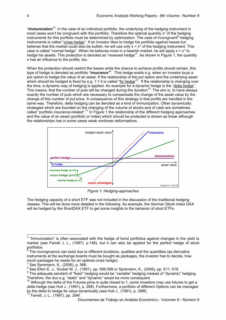
“immunization”5. In the case of an individual portfolio, the underlying of the hedging instrument in most cases won’t be congruent with this portfolio. Therefore the optimal quantity x* of the hedging instruments for this portfolio must be determined by optimization. The case of incongruent6 hedging instruments is called “cross hedge”. If an investor likes to hedge his portfolio against losses but believes that the market could also be bullish, he will use only x < x* of the hedging instrument. This case is called “normal hedge”. When he believes more in a bearish market, he will apply x > x* to hedge his assets. This protection is denoted as “reversed hedge”7. As shown in Figure 1, the quantity x has an influence to the profits, too.

When the protection should restrict the losses while the chance to achieve profits should remain, this type of hedge is denoted as portfolio “insurance”8. This hedge exists e.g. when an investor buys a put option to hedge the value of an asset. If the relationship of the put option and the underlying asset which should be hedged is fixed by e.g. 1:1 it is called “fix hedge”9. If the relationship is changing over the time, a dynamic way of hedging is applied. An example for a dynamic hedge is the “delta hedge”. This means, that the number of puts will be changed during the duration10. The aim is, to have always exactly the number of puts which are necessary to compensate the change of the asset value by the change of this number of put price. A consequence of this strategy is that profits are handled in the same way. Therefore, delta hedging can be denoted as a kind of immunization. Other dynamically strategies which are founded on the changing of the volume of stocks and of cash are sometimes called “portfolio insurance-related”.11 In Figure 1 the relationship of the different hedging approaches and the value of an asset (portfolio or index) which should be protected is shown as linear although the relationships has in some cases weak nonlinear deformations.

asset unhedged

immunization

asset value

hedged asset value

Hedge-ETF-1.dsf 0709

insurance

perfect hedge

cross hedge (x=x*)normal hedge (x<x*)

reversed hedge (x>x*)

fix hedge

Figure 1: Hedging-approaches

The hedging capacity of a short ETF was not included in the discussion of the traditional hedging classes. This will be done more detailed in the following. As example, the German Stock index DAX will be hedged by the ShortDAX ETF to get some insights to the behavior of short ETFs.

5 “Immunization” is often associated with the hedge of bond portfolios against changes in the yield to market (see Farrell J. L., (1997), p.146), but it can also be applied for the perfect hedge of stock portfolios. 6 The incongruence can exist due to different durations, qualities and the quantities (as derivative instruments at the exchange boards must be bought as packages, the investor has to decide, how much packages he needs for an optimal cross hedge). 7 See Spremann, K., (2006), p. 566. 8 See Elton E. J., Gruber M. J., (1991), pp. 598,599 or Spremann, K., (2006), pp. 611, 618. 9 The adequate pendant of “fixed” hedging would be “variable” hedging instead of “dynamic” hedging. Therefore, the duo e.g. “static” and “dynamic” would be more consequent. 10 Although the delta of the Futures price is quite closed to 1, some investors may use futures to get a delta hedge (see Hull J., (1991), p. 288). Furthermore, a portfolio of different Options can be managed by the delta to hedge its value dynamically (see Hull J., (1991), p. 288f). 11 Farrell, J. L., (1997), pp. 294f.



5

3. Short Exchange Traded Funds The short ETF called “ShortDAX” was introduced in the German exchange boards at the 6th of June 2007. It is linked to the German Index DAX. The DAX contains stocks of the 30 biggest companies of the country whose stocks are listed in exchange boards. To buy this short ETF, the investor has to pay its price which will be denoted by ShortDAX . The financial institution which issued the ShortDAX now has to make a short selling of the index DAX to create an inverse performance with a bearish character. By doing this the financial institution receives a second time the same amount, the investor paid to it. Therefore, the double value of the ShortDAX can be invested by the financial institution to earn interests for the investor. When the last trading day of the ETF was δ days before t, he will get twice the interest rate it for the time interval (t-δ). During the week, δ =1 and at the weekend δ =2 or 3. The annual interest rate it which constitutes the “interest term” of the equation (1) is the “European Overnight Interest Average” (EONIA) interest rate12 which is linear adapted in (1) to δ days. Besides the interest term, the value ShortDAXt in period t depends on the development of the value of the index DAX in the interval t-δ. This part is called “leverage term”. When the DAXt-δ will have a decrease of 10% in t-δ the ShortDAXt-δ will increase by 10%. The factor of the leverage term would be: (2-90/100) = (2-0.9) = 1.10. When the DAXt-δ will have an increase of 10% in t-δ the reverse will happen to the ShortDAXt-δ . For the leverage factor of -1, the ShortDAXt-δ will rise to the double value, if the price DAXt-δ is falling between t-δ and t to the value of zero13. On the other side, in this term the ShortDAXt-δ will fall to the value zero (in the Leverage Term in (1)), if the price DAXt-δ is rising to the double price between t-δ and t. The sum of the “leverage term” and the “interest term” constitute the value ShortDAXt at time t (see equation (1))14.

δiShortDAXDAXDAXShortDAXShortDAX t

δtδt

tt-δt ⋅⎟

⎠⎞

⎜⎝⎛⋅⋅+⎟⎟

⎠

⎞⎜⎜⎝

⎛⋅−⋅= −

− 360212 . (1)

Leverage Term Interest Term In the following, the value of the short ETF will be denoted by S and the index by I and further more the time step δ is supposed to be δ =1. Then the value in t of the short ETF for one time step is

( )/180ir-1SS tt1-tt +⋅= (2)

In equation (2) rt is the return of the index achieved between t and the last trading day t-1. In the example above, this rate was rt = -0.10. If the initial value is S0, equation (2) can be used to compute S1, S2 etc. After T days, the value of the short ETF is

∏=

⎟⎠

⎞⎜⎝

⎛ +−⋅=T

t

ttT

irSS1

0 1801 . (3)

The value of the Index which starts with I0 will be in T

( )∏=

+⋅=T

ttT rII

10 1 . (4)

12 The EONIA is fixed by the European Central Bank since 1.1.1999. It is the average of all overnight unsecured lending transactions in the interbank market. 13 Higher leverage factors (e.g. -2) can be found for ETFs (e.g. LevDAX (see Deutsche Börse, 2007, p. 23)) but also for Short ETFs (e.g. Ultrashort Dow30 Proshares (see Morgan Stanley, 2007 or Ferri, R. A., (2008), pp. 226f)). The equation (2) for higher leverage factors can be found in the appendix III. 14 See Deutsche Börse, 2007, pp. 24f.



6

4. Hedging with Short ETF

4.1 Immunization by a Perfect Hedge

The value of an asset can be hedged by a short future. If this asset is identical concerning volume, quantity and quality with the underlying of the future, a perfect hedge is possible. Then a risk free payoff is possible like shown by a horizontal line in Figure 2. The payoff level depends on the “basis” as the difference of the spot price pSpot and the futures price pFuture is called. When instead of short futures the way of “short selling” was used for hedging the asset, the payoff is the difference between the interests which can be earned till T and the fee for borrowing the asset.

In both cases the perfect hedge can create a negative payoff, too.

futuresshort

assetlong

risk freepayoff

asset priceat maturity

payoff


pSpot pFuture

Figure 2: Perfect Hedge using futures

Short ETF as hedging instrument can produce a similar fixed payoff, but only, when T=1. Then the payoff is the interest payment it/360. This perfect hedge ht is the sum of its elements IT and ST which were in the beginning equal weighted respective get the same part of the budget (I0 = S0). With the equations (3) and (4) the result of the perfect hedge is

( ) ⎟⎠⎞

⎜⎝⎛ +−⋅++⋅=+=

18011 00

TTTTTT

irSrISIh . (5)

As the short ETF has the character of an investment instrument, 50% of the budget will be invested in I0 and 50% in S0 to immunize the investment against changing index prices. Now, equation (5) can be reduced to

⎟⎠⎞

⎜⎝⎛ +⋅=⎟

⎠⎞

⎜⎝⎛ +−++⋅=

3601100

1801150 TT

TTTiirrh . (6)

From a theoretical point of view (respective in absence of transaction costs) this immunisation can be applied for T > 1. To be every trading day t perfect hedged, the result of ht must be rebalanced to 50% of the actual budget to It and 50% for St. Then the equation (6) must be completed by t-1 interest factors to

∏=

⎟⎠⎞

⎜⎝⎛ +⋅=

T

t

tT

ih1 360

1100 . (7)

In equation (7) the value of the hedge is only dependent on the interest payments and not on the value of the index DAX. But besides the weak simplification that δ =1 a stronger one was supposed to get this result. This stronger simplification ignores the fact of transaction costs.



7

In the following the hedge of the short ETF will depicted by empirical data. As mentioned above, the ShortDAX was introduced at the exchange board at the 6th June 2007. To get values of the last decade (1st of January 2000 to the 24th of April 2009), the return data of the hedge were determined by the values of the DAX and the EONIA. The annual management fee of 0.15% was not integrated in the calculation of the value of the ShortDAX.

Relativ value of the ShortDAX ETF and the DAX

Distanz of 1 trading day; initial value: 1.0

File: ETF-SPSS-Grafiken

1-T-DAX

1,151,101,051,00,95,90

1-T-

Shor

tDAX

1,10

1,05

1,00

,95

,90

,85

Figure 3: Value of the ShortDAX dependent on the DAX with T =1

The immunization for T=1 is depicted in Figure 3. Obviously the value of the ShortDAX depends on the value of the DAX like in the Figure 2 the short futures on the asset value. For every new trading day, the sum of the value of the DAX and the ShortDAX were set to 1 respective 100%. Therefore Figure 3 shows the %-movement of both instruments. Not visible is the small shift of the interest payment. In Figure 4 this payment was depicted for the time

Return of the Hedge and the value of the DAX

Distanz of 1 trading day (>= 1 calendar days); return

File: ETF-SPSS-Graf iken

1-T-DAX

1,21,11,11,01,0,9

1-T-

Ret

urn-

hedg

ed

,0010

,0008

,0006

,0004

,0002

0,0000

Figure 4: Return of the ShortDAX and the relative value of the DAX within one trading day (T=1)

period of one trading day. Compared with Figure 2, the risk free payment is not a horizontal line. Due to different EONIA interest rates i and values δ, this payment is a cloud of points and not a line. But as interest payments are positive, the risk free result is it too. As the time step δ is not always one, higher returns occurred. The highest one of 0.0007958 refers to δ =5 when the EONIA was about 360(0.00079858/5) =5.75% (at 13th of April 2001).

For a longer investment or hedging time T > 1, this immunization of the DAX by the ShortDAX becomes imperfect. Like the Figures 5 shows, the return of the hedge

hT = IT + ST with IT and ST like in (4) respective (3)

was in the last decade for 10 ≤ T ≤ 300 in the range of -6% to +23% while the return of the DAX was between -57% and +82%. The results depend on the size of the time interval T and on the standard deviation of the return of the index (see below). The interval T refers in the computation of Figures 5a to 5e to calendar days and not to trading days. The positive as the negative returns of the hedge are



8

growing by T. The mentioned extreme values can be found in Figure 5e when the time interval was set to T=300. In a shorter time interval e.g. T=50, the hedge hT creates returns between -3% and +8%. The plots of Figure 5 are sickle-shaped. This means, extreme positive returns as well as extreme negative returns of the DAX offer the possibility to get positive returns by the hedge. Surprising are the minima of these sickle shaped clouds. While the minima of the upper side of the cloud seem to be at the point when the DAX return is zero, the minima at the lower side has its position in every Figure when the DAX produces a negative result between 0 and -20%. This can be interpreted as an asymmetric volatility of the hedge: Positive returns of the DAX seem to produce a return of the hedge which has a smaller volatility than negative returns of this index.

Return of the Fix-Hedge and the DAX

Distanz of T=10 days; return


10-T-DAX-Retrun

,9,8,7,6,5,4,3,2,1-,0-,1-,2-,3-,4-,5-,6

10-T

-Ret

run-

Hed

ged

,25

,20

,15

,10

,05

0,00

-,05

-,10

Figure 5a: Return of the DAX and the hedge hT with T = 10

Return of the Hedge and the DAX



50-T-DAX-Return

,9,8,7,6,5,4,3,2,1-,0-,1-,2-,3-,4-,5-,6

50-T

-Ret

urn-

Hed

ge

,25

,20

,15

,10

,05

0,00

-,05

-,10

Figure 5b: Return of the DAX and the hedge hT with T = 50



9




100-T-DAX-Retrun

,9,8,7,6,5,4,3,2,1-,0-,1-,2-,3-,4-,5-,6

100-

T-R

etru

n-H

edge

d

,25

,20

,15

,10

,05

0,00

-,05

-,10

Figure 5c: Return of the DAX and the hedge hT with T = 100




200-T-DAX-Return

,9,8,7,6,5,4,3,2,1-,0-,1-,2-,3-,4-,5-,6

200-

T-R

etur

n-he

dged

,25

,20

,15

,10

,05

0,00

-,05

-,10

Figure 5d: Return of the DAX and the hedge hT with T = 200



File: ETF-SPSS-Graf iken

300-T-Dax-Rendite

,9,8,7,6,5,4,3,2,1-,0-,1-,2-,3-,4-,5-,6

300-

T-R

etur

n-H

edge

d

,25

,20

,15

,10

,05

0,00

-,05

-,10

Figure 5e: Return of the DAX and the hedge hT with T = 300

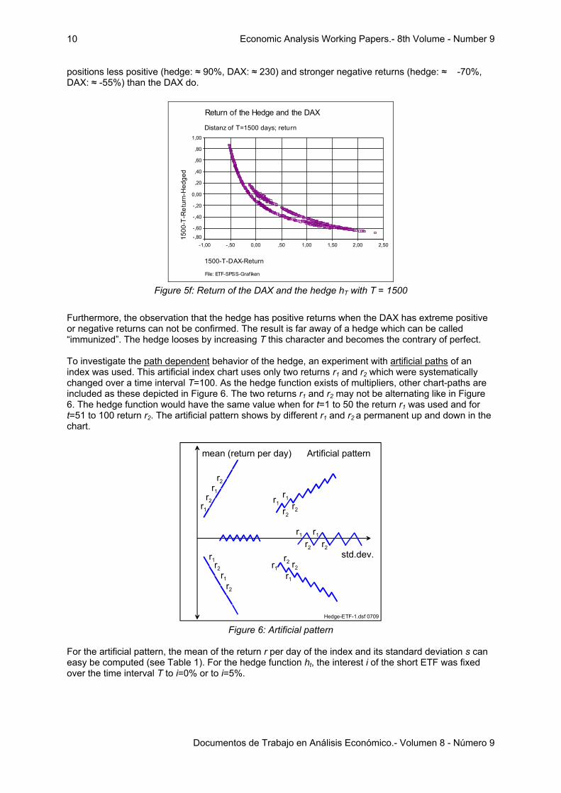
Although hedging instruments were used temporary, the plot was also created for a longer interval of T=1500. In Figure 5f the shape of this plot is not like a sickle. The shape becomes for this T the form of a descending function. It must be remembered, that in Figures 5f (like in Figure 5a-5e) the return of the DAX is compared with the return of the hedge. Obviously the hedge creates in the extreme



10

positions less positive (hedge: ≈ 90%, DAX: ≈ 230) and stronger negative returns (hedge: ≈ -70%, DAX: ≈ -55%) than the DAX do.




1500-T-DAX-Return

2,502,001,501,00,500,00-,50-1,00

1500

-T-R

etur

n-H

edge

d

1,00

,80

,60

,40

,20

0,00

-,20

-,40

-,60

-,80

Figure 5f: Return of the DAX and the hedge hT with T = 1500

Furthermore, the observation that the hedge has positive returns when the DAX has extreme positive or negative returns can not be confirmed. The result is far away of a hedge which can be called “immunized”. The hedge looses by increasing T this character and becomes the contrary of perfect.

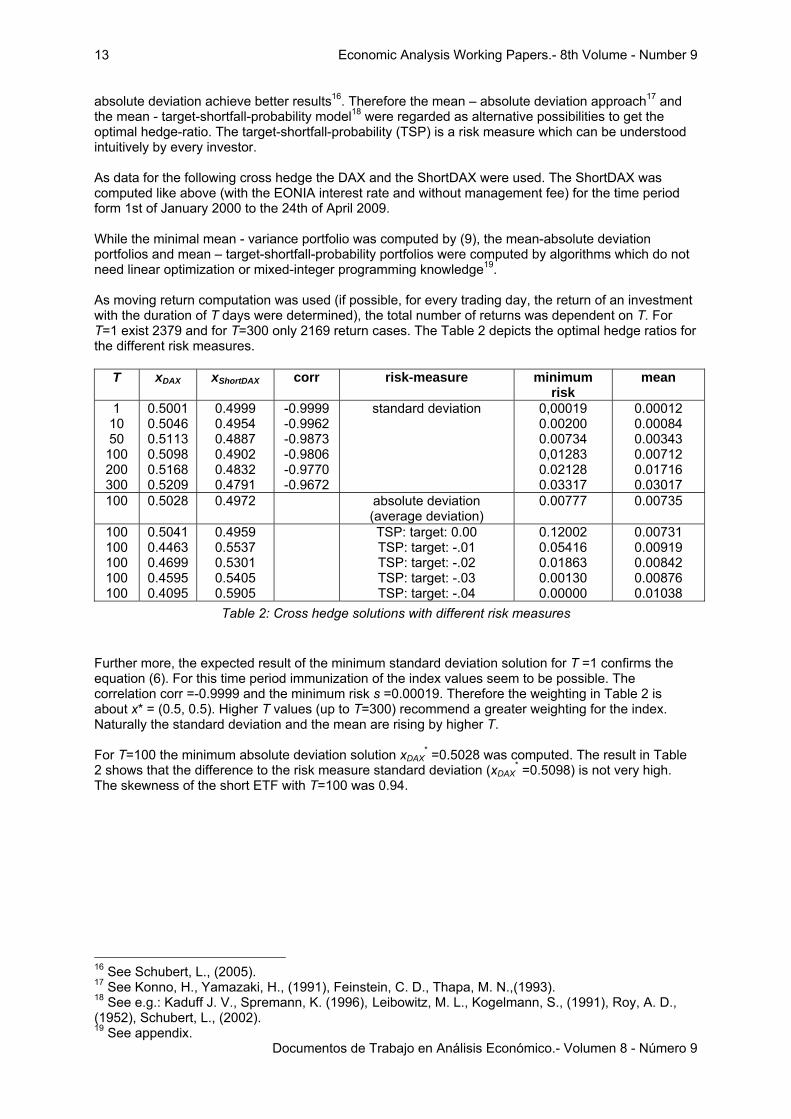
To investigate the path dependent behavior of the hedge, an experiment with artificial paths of an index was used. This artificial index chart uses only two returns r1 and r2 which were systematically changed over a time interval T=100. As the hedge function exists of multipliers, other chart-paths are included as these depicted in Figure 6. The two returns r1 and r2 may not be alternating like in Figure 6. The hedge function would have the same value when for t=1 to 50 the return r1 was used and for t=51 to 100 return r2. The artificial pattern shows by different r1 and r2 a permanent up and down in the chart.

std.dev.

mean (return per day)


r1

r2 r1

r2

r1

r2

r1

r2

r1

r2

r1

r2

r1r2

r1

r2

r1r2

r1r2

Artificial pattern

Figure 6: Artificial pattern

For the artificial pattern, the mean of the return r per day of the index and its standard deviation s can easy be computed (see Table 1). For the hedge function ht, the interest i of the short ETF was fixed over the time interval T to i=0% or to i=5%.



11

Artificial pattern ( )21 rr0.5 +⋅= r (8a) ( )( )2 s 2150 rr. −⋅= (8b) TS.0.5 ⋅+⋅= 50TT I h (8c)

with I0 = S0 = 100 ,

( ) ( )( )22

210 11 /T/T rrI +⋅+⋅=TI ,

⎥⎥⎦

⎤

⎢⎢⎣

⎡⎟⎠⎞

⎜⎝⎛ +−⋅⎟

⎠⎞

⎜⎝⎛ +−⋅=

2

2

2

10 1801

1801

/T/T

TirirSS

Table 1: Return r, standard deviation s and the value of the hedge hT of the artificial pattern

The different return levels of the hedge of the artificial pattern is shown in the two maps of Figures 7a and 7b which axis are built by the mean return r per day of the index and its standard deviation s. The white colored circle in Figure 7a marks the area where most of the real DAX values would be inside due to their r and s. In this example, the interest rate was set to i=0%. According to formula (8a) the mean return r is zero, if r1=-r2. This mean, that the hedge becomes negative, if the chart moves aside. The Figure 7a does not show the exact position or path of the minimum return which exactly is below the zero return line. For the return r2=0.01, i=0% and T=100, the function (8c) has its minimum at r1 =-0.010204 (see appendix IV-4). With (8a) results with r = -0.000102 a position below the zero return line. For higher T these difference is shrinking to r = 0.0. An elevated interest rate i can move the position of the minimum above the zero return line (see formula (IV-4) respective (IV-5)). Besides the confirmation, that aside movements of the index produce negative hedge returns, the simple model shows, that the hedge will achieve the highest returns when the DAX has extreme high positive or extreme negative returns. The return levels of this model within the white cycle are more or less like in the Figure 5c between -4% and 12%. In Figure 7b, the interest rate was set to 5%. This reduces the area of losses within the white circle.

Figure 7a: Return-level of the hedge hT to design pattern I (i=0%, T = 100)

The observed minima of the sickle-shaped plot in Figure 5c occurred when the DAX chart was decreasing some percent within T =100 days with high volatility in the aside movement. This occurred in the time interval from the 10th of October 2008 to the 23rd of January 2009, like in Figure 8 illustrated. The DAX was loosing 8.44% and the hedge 3.44%. The return per day of the index was r =-0.0006 and the volatility s = 0.0350. These characteristics of the hedge minima in the last decade are signed in the Figure 7a and 7b by a yellow point. While under the condition i = 0% the hedge return under the artificial conditions would be about 5%, for i =5%, the return would be below 5% like in reality.



12

Figure 7b: Return-level of the hedge hT to design pattern I (i=5%, T = 100)

DAX Chart

DAX: -8.04%; Hedge: -3.44%


Date: 10.10.08 - 23.01.09

DAX

-val

ue

6000

5500

5000

4500

4000

3500

3000

2500

2000

1500

1000

5000

Figure 8: DAX-Chart with high negative hedge hT return (T = 100)

Finally Figures 7a and 7b depict that losses cannot be explained sufficient only by the time T, the interest i and the standard deviation s. Attention must be paid to the return and path of the index, too.

4.2 Cross Hedge of the underlying The immunization with short ETF seem not to be perfect like e.g. with short futures. Short ETF are to different compared with its underlying especially, when it is used for a long term hedge. A “cross” hedge can serve a saver solution by minimizing the risk of the hedge. But this should be done for the planned hedge period T. As risk measure often the variance of the return is used. The optimal hedge solution15 x1

* is

)r,rcov(ss)r,rcov(sx *

212

22

1

212

11 2 ⋅−+

−= . (9)

In formula (9) the variance of the return of the index respective the short ETF is denoted by s1

2 respective s2

2 and the covariance by cov(r1, r2). The weighting of the short ETF is x2* = 1- x1

*. The return of the index and the short index is always related to a period T within the index should be hedged. For T= 10, 50, 100, 200 and 300, the skewness of the return of the short ETF was 0.77, 1.08, 0.94, 0.85 and 0.77. For very small portfolios with strong skewed returns other risk measures like e.g.

15 See e.g. Grundmann W., Luderer B., (2003), p. 146.



13

absolute deviation achieve better results16. Therefore the mean – absolute deviation approach17 and the mean - target-shortfall-probability model18 were regarded as alternative possibilities to get the optimal hedge-ratio. The target-shortfall-probability (TSP) is a risk measure which can be understood intuitively by every investor.

As data for the following cross hedge the DAX and the ShortDAX were used. The ShortDAX was computed like above (with the EONIA interest rate and without management fee) for the time period form 1st of January 2000 to the 24th of April 2009.

While the minimal mean - variance portfolio was computed by (9), the mean-absolute deviation portfolios and mean – target-shortfall-probability portfolios were computed by algorithms which do not need linear optimization or mixed-integer programming knowledge19.

As moving return computation was used (if possible, for every trading day, the return of an investment with the duration of T days were determined), the total number of returns was dependent on T. For T=1 exist 2379 and for T=300 only 2169 return cases. The Table 2 depicts the optimal hedge ratios for the different risk measures.

T xDAX xShortDAX corr risk-measure minimum risk

mean

1 10 50 100 200 300

0.5001 0.5046 0.5113 0.5098 0.5168 0.5209

0.4999 0.4954 0.4887 0.4902 0.4832 0.4791

-0.9999 -0.9962 -0.9873 -0.9806 -0.9770 -0.9672

standard deviation

0,00019 0.00200 0.00734 0,01283 0.02128 0.03317

0.00012 0.00084 0.00343 0.00712 0.01716 0.03017

100

0.5028 0.4972 absolute deviation (average deviation)

0.00777 0.00735

100 100 100 100 100

0.5041 0.4463 0.4699 0.4595 0.4095

0.4959 0.5537 0.5301 0.5405 0.5905

TSP: target: 0.00 TSP: target: -.01 TSP: target: -.02 TSP: target: -.03 TSP: target: -.04

0.12002 0.05416 0.01863 0.00130 0.00000

0.00731 0.00919 0.00842 0.00876 0.01038

Table 2: Cross hedge solutions with different risk measures

Further more, the expected result of the minimum standard deviation solution for T =1 confirms the equation (6). For this time period immunization of the index values seem to be possible. The correlation corr =-0.9999 and the minimum risk s =0.00019. Therefore the weighting in Table 2 is about x* = (0.5, 0.5). Higher T values (up to T=300) recommend a greater weighting for the index. Naturally the standard deviation and the mean are rising by higher T.

For T=100 the minimum absolute deviation solution xDAX

* =0.5028 was computed. The result in Table 2 shows that the difference to the risk measure standard deviation (xDAX

* =0.5098) is not very high. The skewness of the short ETF with T=100 was 0.94.

16 See Schubert, L., (2005). 17 See Konno, H., Yamazaki, H., (1991), Feinstein, C. D., Thapa, M. N.,(1993). 18 See e.g.: Kaduff J. V., Spremann, K. (1996), Leibowitz, M. L., Kogelmann, S., (1991), Roy, A. D., (1952), Schubert, L., (2002). 19 See appendix.



14

Mean-Target-Shortfall Portfolios

T=100, EONIA

File: DAX-Cross-H

TSP

,5,4,3,2,10,0-,1

Ret

urn-

100

T

,03

,02

,01

0,00

-,01

Target

,0000

-2,0000

-4,0000

Figure 10: Cross hedge with TSP

By the third risk measure TSP different targets solutions were determined for the case T=100. While the solution in the case of τ =0.0 was between the optima of the other risk measures, to avoid negative results (τ =-.01 to τ =-.04) lower weightings (0.44 – 0.41) for the index were recommended (see Table 2). Obviously in the example a greater part of short ETF is necessary to reduce negative returns of the hedge. For the target τ =-0.04 the optimal TSP is zero. For three targets the mean-TSP portfolios are depicted in Figure 10. The curve of the target τ =0.0 shows, that changing the optimal solution will cause a strong elevation of the TSP. 4.3 Cross hedge of a portfolio In the following example a cross hedge of a small portfolio with 5 stocks arbitrary selected out of the German HDAX (Adidas-Salomon AG, BASF AG, Aixtron AG, Allianz AG, Arcandor AG) is depicted. These n =5 stocks were equal weighted mixed at the beginning 4th January 2000. The ShortDAX ETF was applied for hedging the value of this portfolio. The ShortDAX ETF was artificial generated like in the cross hedge above. The optimal hedge was determined for the risk measures variance, absolute deviation and TSP. As moving return computation was used with T=360, the total number of data cases was 2124.

xPortfolio xShortDAX risk-measure minimum risk mean 0.48511 0.51489 standard deviation 0.078526 0.04013 0.47889 0.52111 absolute deviation

(average deviation) 0.064021 0.04055

0.45493 0.48766 0.46261

0.54507 0.51234 0.53739

TSP: target: 0.00 TSP: target: -0.05 TSP: target: -0.10

0.29426 0.16761 0.01318

0.04215 0.03996 0.04164

Table 3: Cross hedge solutions with different risk measure

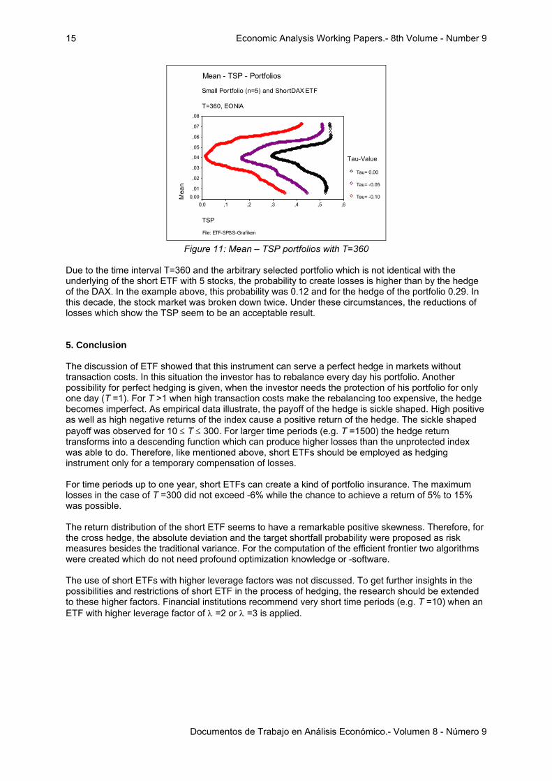
For the determination of the TSP three different targets were applied: τ =0, τ =-5 and τ =-10 to get the Mean-TSP portfolios of the hedge. The minimal risk solution of the three risk measures are depicted in the Table 3. The skewness of the return of the ShortDAX was 0.6549. The correlation between the returns of the small portfolio and the return of the shortDAX-ETF is -0.87. The optimal hedge in the case of the standard deviation as risk measure is different compared with the solution of the absolute deviation or TSP. To avoid negative results (τ =0.0), the alternative risk measures recommend higher weightings xShortDAX. To protect the hedge against losses below -10%, the TSP (τ =-0.10) proposes xShortDAX = 0.53739. For this target, the TSP would be 0.013.



15

Mean - TSP - Portfolios

Small Portfolio (n=5) and ShortDAX ETF

T=360, EONIA


TSP

,6,5,4,3,2,10,0

Mea

n

,08

,07

,06

,05

,04

,03

,02

,010,00

Tau-Value

Tau= 0.00

Tau= -0.05

Tau= -0.10

Figure 11: Mean – TSP portfolios with T=360

Due to the time interval T=360 and the arbitrary selected portfolio which is not identical with the underlying of the short ETF with 5 stocks, the probability to create losses is higher than by the hedge of the DAX. In the example above, this probability was 0.12 and for the hedge of the portfolio 0.29. In this decade, the stock market was broken down twice. Under these circumstances, the reductions of losses which show the TSP seem to be an acceptable result.

5. Conclusion The discussion of ETF showed that this instrument can serve a perfect hedge in markets without transaction costs. In this situation the investor has to rebalance every day his portfolio. Another possibility for perfect hedging is given, when the investor needs the protection of his portfolio for only one day (T =1). For T >1 when high transaction costs make the rebalancing too expensive, the hedge becomes imperfect. As empirical data illustrate, the payoff of the hedge is sickle shaped. High positive as well as high negative returns of the index cause a positive return of the hedge. The sickle shaped payoff was observed for 10 ≤ T ≤ 300. For larger time periods (e.g. T =1500) the hedge return transforms into a descending function which can produce higher losses than the unprotected index was able to do. Therefore, like mentioned above, short ETFs should be employed as hedging instrument only for a temporary compensation of losses. For time periods up to one year, short ETFs can create a kind of portfolio insurance. The maximum losses in the case of T =300 did not exceed -6% while the chance to achieve a return of 5% to 15% was possible. The return distribution of the short ETF seems to have a remarkable positive skewness. Therefore, for the cross hedge, the absolute deviation and the target shortfall probability were proposed as risk measures besides the traditional variance. For the computation of the efficient frontier two algorithms were created which do not need profound optimization knowledge or -software. The use of short ETFs with higher leverage factors was not discussed. To get further insights in the possibilities and restrictions of short ETF in the process of hedging, the research should be extended to these higher factors. Financial institutions recommend very short time periods (e.g. T =10) when an ETF with higher leverage factor of λ =2 or λ =3 is applied.



16

6. References [1] Crama, Y., Schyns, M., (2003), Simulated annealing for complex portfolio optimization problems,

European Journal for Operation Research 150, pp 546-571.

[2] Deutsche Börse, (2007): Leitfaden zu den Strategieindizes der Deutschen Börse, Ver. 1.10, July 2007.

[3] Elton, E. J., Gruber, M. J., (1991), Modern Portfolio Theory and Investment Analysis, 4th edition, Wiley, New York.

[4] Farrell J. L., (1997), Portfolio-Management, Mc Graw Hill, New York.

[5] Feinstein, C. D., Thapa, M. N., (1993), A Reformation of a Mean-Absolute Deviation Portfolio Optimization Model, Management Science, Vol. 39, pp 1552-1553.

[6] Ferri, R. A., (2008), The ETF Book, John Wiley and Sons.

[7] Grundmann, W., Luderer B., (2003), Formelsammlung Finanzmathematik, Versicherungsmathematik, Wertpapieranalyse, Teubner.

[8] Hehn, E. (ed.), (2005), Exchange Traded Funds, Structure, Regulation and Application of a New Fund Class, Springer.

[9] Hull, J., (1991), Introduction to Futures an Options Markets, Prentice-Hall.

[10] Kaduff, J. V., Spremann, K., (1996), Sicherheit und Diversikation bei Shortfall-Risk, zfbf 48, September, pp 779-802.

[11] Konno, H., Yamazaki, H., (1991), Mean – Absolute Deviation Portfolio Optimization Model and its Applications to Tokyo Stock Markets, Management Science, Vol. 37, May, pp 519-531.

[12] Leibowitz, M. L., Kogelmann, S., (1991), Asset allocation under shortfall constraints, The Journal of Portfoliomanagement, pp 18-23.

[13] Morgan Stanley, (2007), Exchange-Trades Funds US Equity – Doubling Up or Doubling down with Leveraged ETFs, Oktober 11.

[14] Roy, A. D., (1952), Safety – First and the Holding of Assets, Econometrica, Vol. 20, pp 431-449.

[15] Rudolf, M., (1994), Efficient Frontiere and Shortfall Risk, Finanzmarkt und Portfolio Management, Ausgabe 1, pp 88-101.

[16] Schubert, L., (2002), Portfolio Optimization with Target-Shortfall-Probability-Vector, Economics Analysis Working Papers, Vol. 1 No 3, 2002, ISSN 15791475.

[17] Schubert, L., (2005), Performance of linear portfolio optimization, Universidad de Costa Rica – Centro de Investigación en Matemática Pura y Aplicada, CIMPA-01-2005, ISSN 1409-3820, Mayo 2005.

[18] Singleton, C., (2004), Core-Satellite Portfolio Management: A Modern Approach to Professionally Managed Funds, McGraw-Hill.

[19] Spremann, K., (2006), Portfoliomanagement, Oldenbourg, München.

[20] Wiandt, J., McClatchy, W., (2002), Exchange Traded Funds, John Wiley and Sons.



17

Appendix The computation on optimal hedge ratios is concentrated to the risk measure variance, although the absolute deviation and the target-shortfall-probability (TSP) offer in the case of skewed distributions better estimator. The computed short ETFs had always remarkable high positive skewness. Therefore, the use of other risk measures than the variance is recommended. The use of different targets offers additional information about the TSP risk of the hedge. To enable the computation of mean – absolute-deviation portfolios or of the mean- TSP portfolios without linear optimization knowledge or mixed integer programming experiences two algorithms were created to determine the optimal hedge (see appendix I and II). In appendix III, the computation of reverse ETFs with higher leverage factor is depicted. The minimal hedge of the artificial function (8c) of Table 1 is computed in appendix VI.

I) Algorithm for hedging a portfolio with minimal absolute-deviation The return of a portfolio respective of the hedging-instrument (e.g. ShortDAX) is denoted by r1t respective r2t over t=1, …, m time intervals. To get the minimal absolute-deviation portfolio the following stochastic programming algorithm with 3 steps can be used. The first determines the absolute deviation o1t respective o2t in each time interval. These values are used in the next step to compute the weightings qt of the portfolio (respective 1-qt of the hedging instrument) when the sign of the absolute deviation is changing. Additional, the direction of this change is determined by pt. To do this computations, the different time intervals have to be classified into sets O++, …, O-- according to the sign of the absolute deviations o1t and o2t. In the third step, the time intervals and corresponding data were completed by q0 =0 and qm+1=1 and ranked to get q0 ≤ q1 ≤ … qm ≤ qm+1. The absolute deviation of the hedge in t can also be written as x·o1t + (1-x)·o2t = x·(o1t – o2t) + o2t with x = qt. The second form was applied to get qt in step no. 2 and to compute the absolute deviation AbsDev(x)= x·St

(1) + St(2). The variable St

(1) represents the sum of the variable part and St(2) the sum of the fix part.

Both variables are determined by a recursive way. For the weighting x =qt =0, only the fix part is important for the computation of the AbsDev(0). Therefore, in equation (I-3) the determination of S0

(1) (with q0= 0) would not be necessary but of S1

(1) (if q1> 0). Starting by x =q0 =0 the AbsDev(x) can be computed until x =1 to get the complete frontier of possible hedges or only until the minimum hedge is found like it is proposed in the third step. In the following the algorithm to get a minimal absolute deviation portfolio is illustrated:

1.) Compute the deviations of the mean oit = rit - µi for t=1, …, m and i=1, 2. 2.) Define the following sets: { }00/ 21 ≥∧≥=++

tt ootO , { }00 21 <∧<=−−tt oo/tO ,

{ }00 21 <∧≥=−+tt oo/tO , { }00 21 ≥∧<=+−

tt oo/tO and compute threshold values for t=1, …, m

{ }

⎪⎪⎪

⎩

⎪⎪⎪

⎨

⎧

∈+−

∪∈

∈−

−

=+−

−−++

−+

Otifoo

oOOtif

Otifoo

o

q

tt

t

tt

t

t

21

2

21

2

0 (I-1)

Set q0 = 0 and qm+1=1. Let the value pt (t=0, …, m+1) be

⎪⎩

⎪⎨

⎧

∈+∈−

= −+

+−

.elseOtifOtif

pt

011

(I-2)

3.) Build a rank order of the threshold values qt that q0 ≤ q1 ≤ … qm ≤ qm+1. Determine the start values



18

∑∑−+−−+−++ ∪∈∪∈

−−−==}OO{t

tt}OO{t

tt)()( )oo()oo(SS 2121

11

10 and (I-3)

∑∑−+−−+−++ ∪∈∪∈

−==}OO{t

t}OO{t

t)()( ooSS 22

21

20

and compute the absolute deviation for x = qt (for t=0, …, m+1) by )(

t)(

tt SSx)qx(AbsDev 21 +⋅== (I-4)

with )oo(pSS ttt)(

t)(

t 2111

1 2 −⋅⋅+=+ and tt)(

t)(

t opSS 222

1 2 ⋅⋅+=+ .

Terminate if AbsDev(x=qt-1) < AbsDev(x=qt) with x* = (x, 1-x)* = (qt-1, 1-qt-1) or if AbsDev(x=qm) > AbsDev(x=qm+1) with x* = (x, 1-x)* = (1, 0).

The advantages of the algorithm are: • No linear optimizer or optimization knowledge is necessary; • The number of periods m nearly does not restrict the algorithm; • The values x =qt offer the computation of the exact corners of the efficient curve and

therefore the complete information about its path (see left side of Figure IIb). In contrast the linear optimization approach20 only alternates the mean to get an approximation of the efficient frontier.

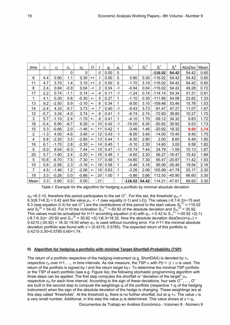
In the computation of the following example, the parameter t is used, to build the index of the rank order over the m=20 time periods according to the different thresholds qt. The example in Table I shows the return of two stocks (e.g. a portfolio and of a hedging instrument). The rank order of to the threshold values (see I-1) is used (see qt respective rank t). Therefore, the time column is not increasing. The different sets O++ etc. can be recognised in the columns O. For example in time period 18 (resp. t=10), the value o1t = -8.7 < 0 and

Mean - Absolute-Deviation Portfolios

Example with m=20


Absolute Deviation

706050403020100

Mea

n

3,5

3,0

2,5

2,0

1,5

1,0

,5

Figure I: Example for Mean - Absolute-Deviation Portfolios with m=20

20 See Konno, H., Yamazaki, H., (1991), Feinstein, C. D., Thapa, M. N., (1993).



19

time r1 r2 o1 o2 O t qt pt S01 S0

2 St1 St

2 AbsDev Mean 0 0 0 0.00 0 -116.02 54.42 54.42 0.60

6 4.4 0.90 1.1 0.30 ++ 1 0.00 0 0.80 0.30 -116.02 54.42 54.42 0.6011 4.7 3.70 1.4 3.10 ++ 2 0.00 0 -1.70 3.10 -116.02 54.42 54.42 0.608 2.4 0.64 -0.9 0.04 -+ 3 0.04 -1 -0.94 0.04 -116.02 54.42 49.28 0.7217 2.2 0.74 -1.1 0.14 -+ 4 0.11 -1 -1.24 0.14 -114.14 54.34 41.31 0.911 4.1 0.30 0.8 -0.30 +- 5 0.27 1 -1.10 0.30 -111.66 54.06 23.82 1.3313 9.2 -2.50 5.9 -3.10 +- 6 0.34 1 -9.00 3.10 -109.46 53.46 15.78 1.5314 -2.4 4.33 -5.7 3.73 -+ 7 0.40 -1 -9.43 3.73 -91.47 47.27 11.07 1.6712 -0.7 3.34 -4.0 2.74 -+ 8 0.41 -1 -6.74 2.74 -72.60 39.80 10.27 1.703 5.7 -1.10 2.4 -1.70 +- 9 0.41 1 -4.10 1.70 -59.12 34.32 9.83 1.7218 -5.4 6.90 -8.7 6.30 -+ 10 0.42 -1 -15.00 6.30 -50.92 30.92 9.53 1.7315 5.3 -0.86 2.0 -1.46 +- 11 0.42 1 -3.46 1.46 -20.92 18.32 9.50 1.742 -1.3 4.00 -4.6 3.40 -+ 12 0.43 -1 -8.00 3.40 -14.00 15.40 9.45 1.754 6.8 -2.20 3.5 -2.80 +- 13 0.44 1 -6.30 2.80 2.00 8.60 9.49 1.8016 6.1 -1.70 2.8 -2.30 +- 14 0.45 1 -5.10 2.30 14.60 3.00 9.58 1.829 -5.0 8.04 -8.3 7.44 -+ 15 0.47 -1 -15.74 7.44 24.79 -1.59 10.13 1.8720 5.7 -1.60 2.4 -2.20 +- 16 0.48 1 -4.60 2.20 56.27 -16.47 10.42 1.895 10.8 -6.70 7.5 -7.30 +- 17 0.49 1 -14.80 7.30 65.47 -20.87 11.42 1.9310 5.6 -2.56 2.3 -3.16 +- 18 0.58 1 -5.46 3.16 95.06 -35.46 19.54 2.167 4.5 -1.46 1.2 -2.06 +- 19 0.63 1 -3.26 2.06 105.98 -41.78 25.17 2.3019 3.3 -0.26 0.0 -0.86 +- 20 1.00 1 -0.86 0.86 112.50 -45.90 66.60 3.30

Mean 3.3 0.60 0.0 0.00 21 -116.02 54.42 114.21 -47.61 66.60 3.30Table I: Example for the algorithm for hedging a portfolio by minimal absolute deviation

o2t =6.3 >0, therefore this period participates to the set O-+. For this set, the threshold q10 = 6.3/(8.7+6.3) = 0.42 and the value p11 = -1 (see equality (I-1) and I-2)). The values (-8.7-6.3)=-15 and 6.3 (see equation (I-3) for set O-+) are the contributions of this period to the start values S0

(1) =-116.02 and S0

(2) = 54.42. For t=10 the inclination S10(1) =-50.92 of the absolute deviation and S10

(2) = 30.92. This values must be actualized for t=11 according equation (I-4) with q11 = 0.42 to S11

(1) =-50.92 +2(-1) (-8.7-6.3))= -20.92 and S11

(2) = 30.92 +2(-1)6.3=18.32. Now the absolute deviation AbsDev(x=q11) = 0.4215 (-20.92) + 18.32 =9.50 when q11 is used without rounding error. For t=11 the minimal absolute deviation portfolio was found with x*= (0.4215, 0.5785). The expected return of this portfolio is 0.4215·3.30+0.5785·0.60=1.74. II) Algorithm for hedging a portfolio with minimal Target-Shortfall-Probability (TSP) The return of a portfolio respective of the hedging-instrument (e.g. ShortDAX) is denoted by r1t respective r2t over t=1, …, m time intervals. As risk measure, the TSP α with P(r < τ) ≤ α is used. The return of the portfolio is signed by r and the return target byτ. To determine the minimal TSP portfolio or the TSP of each portfolio (see e.g. Figure IIa), the following stochastic programming algorithm with three steps can be applied. The first step computes the shortfall or “deviation of the target” o1t respective o2t for each time interval. According to the sign of these deviations, four sets O++, …, O-- are built in the second step to compute the weightings qt of the portfolio (respective 1-qt of the hedging instrument) when the sign of the absolute deviation of the hedge is changing. These weightings are at this step called “thresholds”. At the threshold qt, there is no further shortfall, but at qt +ε. The value ε is a very small number. Additional, in this step the value pt is determined. This value shows at x = qt,



20

whether the sign of the deviation of the hedge x·o1t + (1-x)·o2t = x·(o1t – o2t) + o2t changes form positive to negative (pt = +1) or reverse (pt = -1). The value pt = 0 is fixed, if the sign do not change for x∈[0, 1]. In the third step, the time intervals and corresponding data were completed by q0 =0 and qm+1=1 and ranked to get q0 ≤ q1 ≤ … qm ≤ qm+1. As the deviation of the hedge referring the target has a variable part x·(o1t – o2t) and a fix part o2t for x =q0 =0 only the fix part is responsible for shortfalls. These occur in time intervals t of the sets O-- and O+-. For x = qt >0 this number of cases of target shortfalls TS(x) must be increased or reduced by the corresponding pt of the next threshold. The TSP(x) is computed by the ratio TS/m. To get the complete frontier of possible hedges this computation begins at x = qm+1 =1 and ends at q0 =0. A minimal hedge is the solution with minimal TSP which may not be unique.

In the following the three steps to find a minimal TSP portfolio is depicted:

1.) Compute the deviations of the target oit = rit - τ for t=1, …, m and i=1, 2. 2.) Define the following sets: { }00 21 ≥∧≥=++

tt oo/tO , { }00 21 <∧<=−−tt oo/tO ,

{ }00 21 <∧≥=−+tt oo/tO , { }00 21 ≥∧<=+−

tt oo/tO let the threshold values q0 = 0 and qm+1=1 and compute the other thresholds by

{ }

⎪⎪⎪

⎩

⎪⎪⎪

⎨

⎧

∈++−

∪∈

∈−

−

=+−

−−++

−+

.Otifoo

oOOtif

Otifoo

o

q

tt

t

tt

t

t

ε21

2

21

2

0 (II-1)

In (II-1) ε is a very small number. Let the value pt (t=0, …, m+1) be

⎪⎩

⎪⎨

⎧

∈−∈+

= −+

+−

.elseOtifOtif

pt

011

3.) Build a rank order of the threshold values qt that q0 ≤ q1 ≤ … qm ≤ qm+1. Compute the target-

shortfalls TS(x) by { }

⎪⎩

⎪⎨⎧

+==

+

∪==

−

−+−−

110

1m,...,t

tifif

p)q(TS

OO)qx(TS

tt

t (II-2)

and the target-shortfall probability beginning with TSP(x=1)=TS(qm+1)/m

⎩⎨⎧

=≠

==+

+

+ 1

1

1 tt

tt

t

tt qq

qqifif

)q(TSPm/)q(TS

)qx(TSP

The minimal TSP portfolio is not always found if TSP(x=qt-1) < TSP(x=qt) with the solution x* = (qt-1, 1-qt-1)*. Therefore, all TSP(qt) values must be considered to get the optimal solution x*. The advantages of the algorithm are:

• No Branch and Bound optimizer and mixed integer optimisation knowledge are necessary; • The number of period m nearly does not restrict the algorithm; • More different targets can be regarded, too; • The exactly return interval for each single TSP can be determined (see vertical lines on

the right side of Figure IIb). For two thresholds qt ≠ qt+1 the return interval is the set {r / r = x·r1 +(1-x)·r2; qt ≤ x < qt+1}.

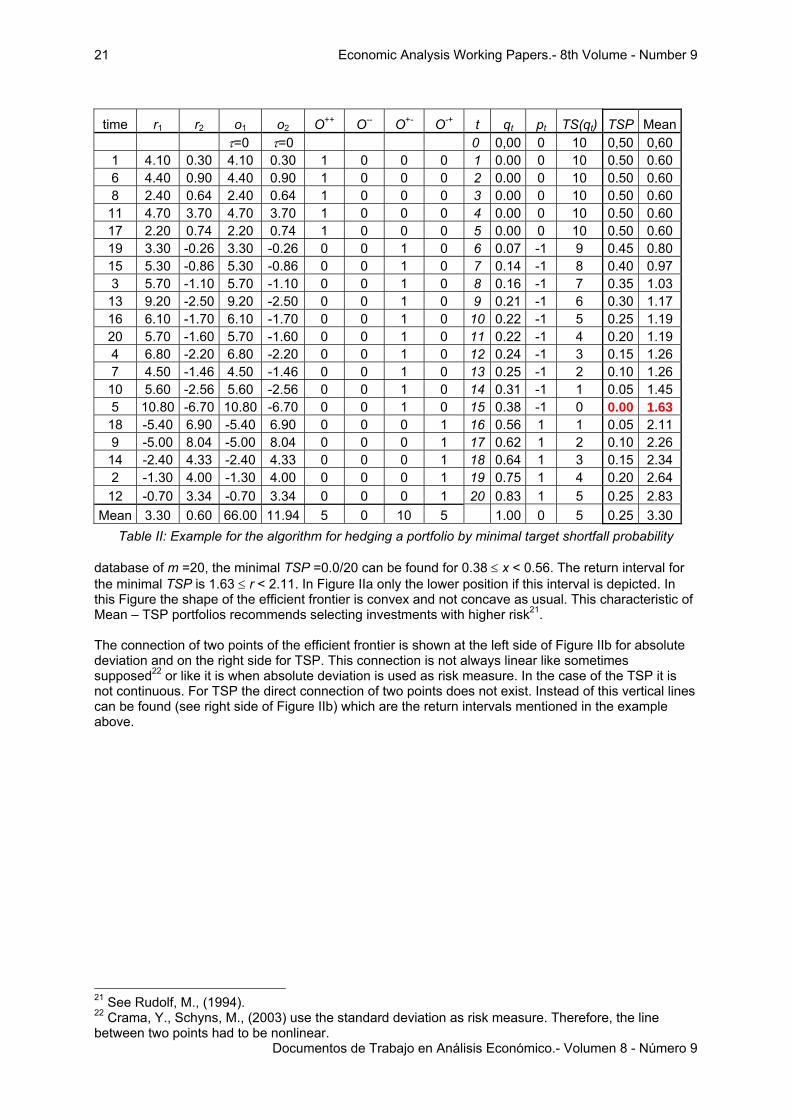
In Table II the return data of the example of Table I with m =20 were used to illustrate the application of the algorithm. As target τ = 0 was selected. The three steps determine the solutions for x =qt which are in the two columns at the right side of Table II. The target shortfall variable TS(q0)=10 starts with the sum of the columns O--and O+- and according to (II-2) TS(q14)=1. The value TS(q15)= TS(q14)+p15=1+(-1)=0 with q15 = 0.38. Due to the small



21

time r1 r2 o1 o2 O++ O-- O+- O-+ t qt pt TS(qt) TSP Mean τ=0 τ=0 0 0,00 0 10 0,50 0,60 1 4.10 0.30 4.10 0.30 1 0 0 0 1 0.00 0 10 0.50 0.60 6 4.40 0.90 4.40 0.90 1 0 0 0 2 0.00 0 10 0.50 0.60 8 2.40 0.64 2.40 0.64 1 0 0 0 3 0.00 0 10 0.50 0.60 11 4.70 3.70 4.70 3.70 1 0 0 0 4 0.00 0 10 0.50 0.60 17 2.20 0.74 2.20 0.74 1 0 0 0 5 0.00 0 10 0.50 0.60 19 3.30 -0.26 3.30 -0.26 0 0 1 0 6 0.07 -1 9 0.45 0.80 15 5.30 -0.86 5.30 -0.86 0 0 1 0 7 0.14 -1 8 0.40 0.97 3 5.70 -1.10 5.70 -1.10 0 0 1 0 8 0.16 -1 7 0.35 1.03 13 9.20 -2.50 9.20 -2.50 0 0 1 0 9 0.21 -1 6 0.30 1.17 16 6.10 -1.70 6.10 -1.70 0 0 1 0 10 0.22 -1 5 0.25 1.19 20 5.70 -1.60 5.70 -1.60 0 0 1 0 11 0.22 -1 4 0.20 1.19 4 6.80 -2.20 6.80 -2.20 0 0 1 0 12 0.24 -1 3 0.15 1.26 7 4.50 -1.46 4.50 -1.46 0 0 1 0 13 0.25 -1 2 0.10 1.26 10 5.60 -2.56 5.60 -2.56 0 0 1 0 14 0.31 -1 1 0.05 1.45 5 10.80 -6.70 10.80 -6.70 0 0 1 0 15 0.38 -1 0 0.00 1.63 18 -5.40 6.90 -5.40 6.90 0 0 0 1 16 0.56 1 1 0.05 2.11 9 -5.00 8.04 -5.00 8.04 0 0 0 1 17 0.62 1 2 0.10 2.26 14 -2.40 4.33 -2.40 4.33 0 0 0 1 18 0.64 1 3 0.15 2.34 2 -1.30 4.00 -1.30 4.00 0 0 0 1 19 0.75 1 4 0.20 2.64 12 -0.70 3.34 -0.70 3.34 0 0 0 1 20 0.83 1 5 0.25 2.83

Mean 3.30 0.60 66.00 11.94 5 0 10 5 1.00 0 5 0.25 3.30 Table II: Example for the algorithm for hedging a portfolio by minimal target shortfall probability

database of m =20, the minimal TSP =0.0/20 can be found for 0.38 ≤ x < 0.56. The return interval for the minimal TSP is 1.63 ≤ r < 2.11. In Figure IIa only the lower position if this interval is depicted. In this Figure the shape of the efficient frontier is convex and not concave as usual. This characteristic of Mean – TSP portfolios recommends selecting investments with higher risk21. The connection of two points of the efficient frontier is shown at the left side of Figure IIb for absolute deviation and on the right side for TSP. This connection is not always linear like sometimes supposed22 or like it is when absolute deviation is used as risk measure. In the case of the TSP it is not continuous. For TSP the direct connection of two points does not exist. Instead of this vertical lines can be found (see right side of Figure IIb) which are the return intervals mentioned in the example above.

21 See Rudolf, M., (1994). 22 Crama, Y., Schyns, M., (2003) use the standard deviation as risk measure. Therefore, the line between two points had to be nonlinear.



22

Mean - Target-Shortfall-Probability Portfolios

Example with m= 20 and Target = 0


Target-Shortfall-Probability

,6,5,4,3,2,10,0-,1

Mea

n

3,5

3,0

2,5

2,0

1,5

1,0

,5

Figure IIa: Example for Mean – TSP portfolios with m =20


absolute deviation target-shortfall probabilty.

return return

Figure IIb: Efficient frontier and risk measure

III) Short ETFs with higher leverage factor Short ETF exist with different leverage factor λ, too. In the value of a short ETF is

δiS)(λIIλ)(λSS t

τtτt

tt-τt ⋅⎟

⎠⎞

⎜⎝⎛⋅⋅++⎟⎟

⎠

⎞⎜⎜⎝

⎛⋅−+⋅= −

− 36011 . (III-1)

Leverage Term Interest Term

The leverage factor λ is without sign respective λ = 1, 2 or 3. With higher leverage factors λ = 2 or λ = 3 the risk to loose rises, too. To get the higher leverage the issuer of the short ETF has to sell twice or three times the underlying index. Therefore the accruing of interests rises by the same factor. The use of the return per day rt of the index offers a form of (III-1): ( ) ( )( )δ/iλr-λSS ttt-t ⋅⋅++⋅⋅= 360111 . (III-2)



23

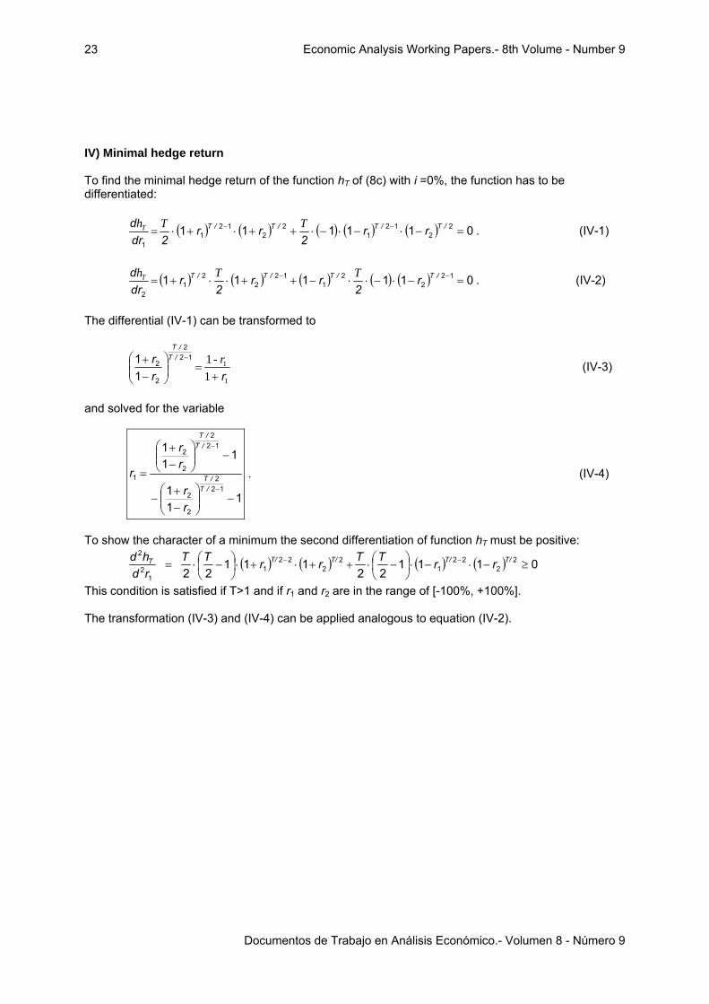
IV) Minimal hedge return To find the minimal hedge return of the function hT of (8c) with i =0%, the function has to be differentiated:

( ) ( ) ( ) ( ) ( ) 011111 22

121

22

121

1

=−⋅−⋅−⋅++⋅+⋅= −− /T/T/T/T rr2

rr2rd

d TT hT . (IV-1)

( ) ( ) ( ) ( ) ( ) 011111 122

21

122

21

2

=−⋅−⋅⋅−++⋅⋅+= −− /T/T/T/T r2

rr2

rrd

d TT hT . (IV-2)

The differential (IV-1) can be transformed to

1

1

11

rrr /T

/T

+=⎟⎟

⎠

⎞⎜⎜⎝

⎛−+ − r-

122

2

2

11 (IV-3)

and solved for the variable

111

111

122

2

2

122

2

2

1

−⎟⎟⎠

⎞⎜⎜⎝

⎛−+

−

−⎟⎟⎠

⎞⎜⎜⎝

⎛−+

=−

−

/T/T

/T/T

rr

rr

r . (IV-4)

To show the character of a minimum the second differentiation of function hT must be positive:

( ) ( ) ( ) ( ) 011122

11122

22

221

22

221

12

2

≥−⋅−⋅⎟⎠⎞

⎜⎝⎛ −⋅++⋅+⋅⎟

⎠⎞

⎜⎝⎛ −⋅= −− T/T/T/T/T rrTTrrTT

rdhd

This condition is satisfied if T>1 and if r1 and r2 are in the range of [-100%, +100%]. The transformation (IV-3) and (IV-4) can be applied analogous to equation (IV-2).