econstorMake Your Publications Visible.

A Service of

zbwLeibniz-InformationszentrumWirtschaftLeibniz Information Centrefor Economics

Herzer, Dierk; Strulik, Holger

Working Paper

Religiosity and income: A panel cointegration andcausality analysis

cege Discussion Papers, No. 168

Provided in Cooperation with:Georg August University of Göttingen, cege - Center for European,Governance and Economic Development Research

Suggested Citation: Herzer, Dierk; Strulik, Holger (2013) : Religiosity and income: A panelcointegration and causality analysis, cege Discussion Papers, No. 168, University of Göttingen,Center for European, Governance and Economic Development Research (cege), Göttingen

This Version is available at:http://hdl.handle.net/10419/79223

Standard-Nutzungsbedingungen:

Die Dokumente auf EconStor dürfen zu eigenen wissenschaftlichenZwecken und zum Privatgebrauch gespeichert und kopiert werden.

Sie dürfen die Dokumente nicht für öffentliche oder kommerzielleZwecke vervielfältigen, öffentlich ausstellen, öffentlich zugänglichmachen, vertreiben oder anderweitig nutzen.

Sofern die Verfasser die Dokumente unter Open-Content-Lizenzen(insbesondere CC-Lizenzen) zur Verfügung gestellt haben sollten,gelten abweichend von diesen Nutzungsbedingungen die in der dortgenannten Lizenz gewährten Nutzungsrechte.

Terms of use:

Documents in EconStor may be saved and copied for yourpersonal and scholarly purposes.

You are not to copy documents for public or commercialpurposes, to exhibit the documents publicly, to make thempublicly available on the internet, or to distribute or otherwiseuse the documents in public.

If the documents have been made available under an OpenContent Licence (especially Creative Commons Licences), youmay exercise further usage rights as specified in the indicatedlicence.

www.econstor.eu

ISSN: 1439-2305

Number 168 – August 2013

Religiosity and Income: A Panel

Cointegration and Causality Analysis

Dierk Herzer, Holger Strulik

Religiosity and Income: A Panel Cointegration andCausality Analysis

Dierk Herzer∗

Holger Strulik†

July 2013

Abstract. In this paper we examine the long-run relationship between religiosity and

income using retrospective data on church attendance rates for a panel of countries

from 1925 to 1990. We employ panel cointegration and causality techniques to control

for omitted variable and endogeneity bias and test for the direction of causality. We

show that there exists a negative long-run relationship between the level of religiosity,

measured by church attendance, and the level of income, measured by the log of GDP

per capita. The result is robust to alternative estimation methods, potential outliers,

sample selection, different measures of church attendance, and alternative specifications

of the income variable. Long-run causality runs in both directions, higher income leads

to declining religiosity and declining religiosity leads to higher income.

Keywords: religiosity; church attendance, income, panel cointegration, causality.

JEL: N30; O11; C23.

∗ Helmut-Schmidt-University Hamburg, Department of Economics, Holstenhofweg 85, 22043 Hamburg, Germany.Email: herzer@hsu-hh.de.† University of Gottingen, Department of Economics, Platz der Gottinger Sieben 3, 37073 Gottingen, Germany;email: holger.strulik@wiwi.uni-goettingen.de.

1. Introduction

Secularization, broadly understood, describes the phenomenon that later born generations

appear to be less religious, revealed, for example, by lower weekly attendance rates at church

(see e.g. Wilson, 2003; Voas 2009). The narrow definition of secularization assigns a cause

to this time trend, inspired by the observation that secularization occurred in the Western

world after the Industrial Revolution and the take off of economic growth (Azzi and Ehrenberg,

1975; Dobbelaere, 1987; Norris and Inglehart, 2004; Bruce, 2011). According to this so called

“secularization hypothesis” improving economic conditions have caused the decline in religiosity

and the decline of demand for religious services. McCleary and Barro (2006a) provide a concise

introduction to the literature on the secularization hypothesis.1

Religious believes and the associated behavior, in turn, may have an in impact on economic

performance. Recent developments in the theory and empirics of economic growth have increas-

ingly focussed on the “fundamental determinants” of growth, comprising culture, geography,

and institutions, which are thought of as causal drivers of the proximate determinants of eco-

nomic growth, comprising physical and human capital accumulation and technological change

(Acemoglu, 2009). Religiosity is certainly an important element of culture but the direction of

causality with respect to growth is a priori unclear. On the one hand, increasing religiosity could

be conducive to economic growth because it encourages trust and trustworthiness (Guiso et al.,

2003) or because it entails an incentive to accumulate human capital (Becker and Woessmann,

2009). On the other hand increasing secularization could be conducive to growth because the

turn towards material values and the promised pleasures from consumption induce increasing

labor supply and capital accumulation (Lipford and Tollison, 2003; Strulik, 2012). Besides the

possibility of forward and backward causation there exists, of course, the possibility that the

decline of religiosity is unrelated to economic growth.

There exist already a few quantitative studies on the income – religiosity nexus. McCleary

and Barro (2006a) found a causal negative effect of income on religious participation and beliefs

across countries, which is also quantitatively important. A one standard deviation increase in

1In principle, church attendance can be seen as a plausible revealed preference for religion because it entails anopportunity costs. Although declining attendance does not necessarily imply that not attending persons stoppedbelieving, it documents that these persons assign less value to religious services. In this sense their religiosityis declining. Church attendance may actually overestimate religiosity because attending could be driven bysecular motives like social capital accumulation. In in any case, attendance is the most widely available and mostfrequently used religiosity variable.

1

log GDP per capita decreases church attendance by 15 percent. McCleary and Barro (2006b)

arrived at similar results. The latter study documents also a significant negative impact of church

attendance on economic growth. Paldam and Gundlach (2013) used the World Value survey

to compile a religiosity index (14 items from “God is very important in life” to “Churches

answer spiritual needs”) and found across countries a causal negative impact of income on

religiosity. On average, religiosity falls by 50 percent when countries pass through the transition

from being underdeveloped to becoming a developed country. Becker and Woessmann (2013)

could not find a causal effect of (teacher-) income on church attendance in Prussia 1886-1911.

Lipford and Tollison (2003) documented a bi-causal negative association of income and religious

participation across US states. Rupasingha and Chilton (2009) used US county level data on

religious adherence and found a causal negative effect of adherence on economic growth. An

increase of religious adherence by one standard deviation would reduces growth by 0.4 percent

per year.

So far, however, little attention has been paid to the time dimension in the analysis of religios-

ity and economic growth. On the one hand this is understandable because data on religiosity was

not available for sufficiently many time periods to allow for a rigorous time series analysis.2 On

the other hand this state of the art is deplorable since both economic growth and the decline of

religiosity (church attendance) are inherently dynamic phenomena. In particular, secularization

is usually not interpreted as differential religiosity across economically diverse countries but as

within-country process along the time-dimension. The question is whether an observable de-

cline in religiosity has been caused be a preceding increase of income (or vice versa) and whether

countries share a common dynamic relationship between religiosity and income.

In the present paper we try to address these questions. We examine the long-run relationship

between religiosity and income using panel cointegration techniques. A feature of cointegration

analysis is that the resulting estimates are robust to a variety of estimation problems that often

plague empirical work, including omitted variables, endogeneity, and measurement errors (see,

e.g., Pedroni, 2007; Herzer, et al., 2012). We identify the direction of causality using Granger-

causality tests and impulse response functions, that is by using techniques which are built upon

the idea that the cause occurred before the effect.

2McCleary and Barro (2006a) compare estimates from World Value Surveys 1981, 1990, and 1995 and from ISSPdata 1991 and 1998 and do not find a significant (autonomous) time trend of church attendance once they controlfor income and other explanatory variables.

2

As variable for religiosity we use the estimated national church attendance rates between

1925 and 1990 provided by Iannaccone (2003). The ingenious idea of Iannaccone’s study is to

estimate historical church attendance rates using contemporary ISSP questionnaires and replies

to inquires on church attendance when the respondents were 11 or 12 years old. Naturally, this

retrospective method could be harmed by different sorts of biases (e.g. age effects or projection

bias). Iannaccone therefore devotes the greater part of his study to carefully demonstrate that

there is no reason for concern. The data stands up to numerous test of internal and external

consistency. For our cointegration analysis we combine the retrospective attendance data, which

is available at five year intervals, with data on GDP per capita from Maddison (2003). Our main

finding is a strong negative impact of economic growth on church attendance.

At first sight our results seemingly disagree with those of Franck and Iannaccone (2009) who

also used the Iannaccone (2003) data and found little support for a causal impact of income

on church attendance. One possible explanation is that the instrument variable technique used

by Franck and Iannaccone did not satisfactorily resolve the problems of reverse causality and

omitted variables. In contrast, our approach does not require exogeneity assumptions nor does

it require the use of instruments. The reason is that, under cointegration, parameter estimates

are superconsistent, implying that endogeneity does not affect the results (Engle and Granger,

1987). The superconsistency property holds even in the presence of omitted stationary variables

and the presence of non-systematic measurement error.

The finding of cointegration between two nonstationary variables implies that there are no

missing relevant nonstationary variables and that no additional nonstationary variables are re-

quired to produce unbiased parameter estimates. While a regression consisting of cointegrated

nonstationary variables has a stationary error term, any omitted nonstationary variable that

is part of the true cointegrating relationship would enter the error term, thereby producing

non-stationary residuals and failure to detect cointegration. Since the cointegration property is

invariant to extensions of the information set, the finding of a particular cointegration relation-

ship in a small set of variables will also hold in an extended variable set. This invariance of the

cointegration property to extensions of the information set implies that the classical omitted

variables problem does not exist under cointegration.

These properties are important in light of the secularization debate because another potential

driver of church attendance could be the diversity of supply of religious services. If this is the

3

indeed case – as argued by Finke and Iannaccone (1993) and other proponents of the religious

supply hypothesis – then it would not bias our results. The inclusion of additional variables

would not destroy the original cointegrating relationship (Lutkepohl, 2007). This is the main

justification to consider small “subsystems” (such as the relationship of church attendance and

income) if the variables are cointegrated. Of course, this means also vice versa that the strong

evidence for a causal impact of income growth on church attendance established in our study

does not refute the religious supply hypothesis. If such a supply channel exist, it would be added

to the set of explanatory variables without affecting the income channel.

The paper is organized as follows. In Section 2.1 we set up the basic empirical model and

discuss some econometric issues. We then describe the data and report summary statistics,

including pre-tests for unit-roots and cointegration (Section 2.2). In Section 3 we present the

empirical analysis. In Section 3.1 we provide estimates of the cointegrating relationship between

religiosity and income, in Section 3.2 we test the robustness of the estimates, and in Section

3.3 we investigate the direction of long-run causality between the two variables. We conclude in

Section 4.

2. Model and Data

2.1. Basic Empirical Model and Econometric Methodology. The basic econometric spec-

ification used to examine the long-run relationship between religiosity and income is a conven-

tional bivariate panel cointegration model of the form

CHURCHit = ai + β log(yit) + ǫit (1)

where i = 1, 2, . . . , N is the country index, t = 1, 2, . . . , T is the time index, and the ai are

country-specific fixed effects. Following previous studies, we use church attendance as our mea-

sure of religiosity (CHURCHit), while income is measured by real GDP per capita (yit). The

income variable is logged, as in most previous studies (see, for example, McCleary and Barro,

2006; Franck and Iannaccone, 2009; Becker and Woessmann, 2013), but in the robustness sec-

tion, we also estimate the model using the non-log-transformed income variable, as in Lipford

and Tollison (2003). Using the log specification allows for an intuitive interpretation of results.

To see this, differentiate (1) and obtain the change of church attendance dCHURCHit as a

4

function of the growth rate of GDP per capita, dgdpit/gdpit. Equation (1) thus stipulates that

changing religiosity is associated with income growth.

We now turn to econometric issues. The first observation is that the underlying variables

are trended; they are nonstationary (as shown in Figures 1 and 2). Given that most economic

time series are characterized by a stochastic rather than deterministic nonstationarity, it is

plausible to assume that the trends in CHURCHit and log(yit) are also stochastic – through

the presence of a unit root – rather than deterministic – through the presence of polynomial time

trends. If this assumption is correct, the linear combination of these integrated (or stochastically

trending) variables must be stationary, or, in the terminology of Engle and Granger (1987),

CHURCHit and log(yit) must be cointegrated. If the two variables are not cointegrated, then

there is no long-run relationship between religiosity and income, and Equation (1) would be a

spurious regression in the sense of Granger and Newbold (1974). Standard regression output

must therefore be treated with extreme caution when variables are nonstationary, since the

estimated results are potentially spurious (see also Eberhardt and Teal, 2013). As shown by

Entorf (1997) and Kao (1999), the tendency for spuriously indicating a relationship may even

be stronger in panel data regressions than in pure time-series regressions. Thus, the necessary

condition for the existence of a non-spurious long-run relationship between CHURCHit and

log(yit) is that the two integrated variables cointegrate.3

A regression consisting of cointegrated variables has the property of superconsistency such

that coefficient estimates converge to the true parameter values at a faster rate than they do

in standard regressions with stationary variables, namely at rate T rather than√T (Stock,

1987). The important point in this context is that the estimated cointegration coefficients are

superconsistent even in the presence of temporal and/or contemporaneous correlation between

the stationary error term, ǫit , and the regressor(s) (Stock, 1987), implying that cointegration

estimates are not biased by omitted stationary variables (see, e.g., Bonham and Cohen, 2001).

The fact that a regression consisting of cointegrated variables has a stationary error term

also implies that no relevant nonstationary variables are omitted. Any omitted nonstationary

variable that is part of the cointegrating relationship would become part of the error term,

3The standard time-series approach is to first-difference the variables to remove the nonstationarity in the dataand to avoid spurious results. However, this approach precludes the possibility of a long-run or cointegratingrelationship in the data and leads to misspecification if a long-run relationship between the levels of the variablesexists (see, e.g., Granger, 1988).

5

thereby producing nonstationary residuals, and thus leading to a failure to detect cointegration

(Everaert, 2011).

If there is cointegration between a set of variables, then this stationary relationship also exists

in extended variable space. In other words, the cointegration property is invariant to model

extensions (see also Lutkepohl, 2007), which is in stark contrast to regression analysis where

one new variable can alter the existing estimates dramatically (Juselius, 2006, p. 11). The

important implication of finding cointegration is that no additional variables are required to

account for the classical omitted variables problem because such a problem does not exist under

cointegration; the result for the long-run relationship between religiosity and income would also

hold if we included additional independent variables in the model (see also Juselius, 1996).

Of course, there are several other factors such as education, fertility, and government ex-

penditure that may be associated with religiosity and/or income. Therefore, adding further

nonstationary variables to the model may, on the one hand, result in further cointegrating rela-

tionships. These, however, would have to be identified and estimated (separately). In particular,

the difficulty is that if there is more than one stationary linear combination of the variables,

identifying restrictions are required to separate the cointegrating vectors. On the other hand,

adding further nonstationary variables to the regression model may result in spurious associ-

ations. More specifically, if a nonstationary variable that is not cointegrated with the other

variables is added to the cointegrating regression, the error term will no longer be stationary.

As a result, the coefficient of the added variable will not converge to zero, as one would expect

of an irrelevant variable in a standard regression (Davidson, 1998). This justifies a reduced-form

model such as Equation (1), given the variables are cointegrated.

The superconsistency of the cointegration estimation also implies that the potential endogene-

ity of the regressors does not affect the estimated long-run coefficients; the estimated long-run

coefficients from reverse regressions should be approximately the inverse of each other due to

the superconsistency (Engle and Granger, 1987). Nevertheless, there are two problems.

First, although the standard least-squares dummy variable estimator is superconsistent under

panel cointegration, it suffers from a second-order asymptotic bias arising from serial correlation

and endogeneity. As a consequence, its t-ratio is not asymptotically standard normal. To

deal with this problem, one has to employ an asymptotically efficient (cointegration) estimator.

Examples of such estimators include panel versions of the dynamic OLS (DOLS) and fully

6

modified ordinary least squares (FMOLS) methods. As shown by Wagner and Hlouskova (2010),

the panel DOLS estimator of Mark and Sul (2003) outperforms other asymptotically efficient

estimators. Therefore, this estimator is preferred here, but in the robustness section we also

present results based on alternative estimation procedures.

Second, although the existence of cointegration implies long-run Granger causality in at least

one direction (Granger, 1988), cointegration says nothing about the direction of the causal re-

lationship between the variables. A statistically significant cointegrating relationship between

CHURCHit and log(yit) does therefore not necessarily imply that, in the long run, changes

in income cause changes in religiosity. The causality may run in the opposite direction, from

CHURCHit to log(yit), or in both directions. The empirical implication is that it is impor-

tant not only to employ an asymptotically efficient cointegration estimator (to account for the

potential endogeneity of income), but also to explicitly test the direction of long-run causality.

As is common practice in testing long-run Granger causality between cointegrated variables, we

use a vector error correction model (VECM) to identify cause and effect in the sense of Granger

(1988).

A final econometric issue is the potential cross-sectional dependence in the regression errors

due to common shocks or spillovers among countries at the same time. Standard panel (cointe-

gration) techniques assume cross-sectional independence and may be biased if this assumption

does not hold. Therefore, we test for cross-sectional dependence in the residuals of the estimated

models using the cross-sectional dependence (CD) test developed by Pesaran (2004). In cases

where we find evidence of cross-sectional dependence, we employ demeaned variables to control

for common effects; that is, in place of CHURCHit and log(yit), we use

CHURCH ′

it = CHURCHit − CHURCHt, CHURCHt ≡ N−1N∑

i=1

CHURCHit (2a)

log(yit)′ = log(yit)− log(yt), log(yt) ≡ N−1

N∑

i=1

log(yit), (2b)

which is equivalent to including time dummies in the model. Moreover, we use a battery of

panel unit root and cointegration tests, including so-called second-generation panel unit root

and cointegration methods that explicitly allow for cross-sectional dependence.

2.2. Data, Unit root and Cointegration Tests. Data on real per capita GDP are taken from

Maddison (2003), available at http://dx.doi.org/10.1787/456125276116. Data on church

7

attendance are from Iannaccone (2003), who uses retrospective survey questions on church at-

tendance rates for respondents and their parents from the International Social Survey Program

to construct average weekly church attendance rate of parents and children in 32 countries be-

tween 1925 and 1990. Attendance of parents is our preferred measure of religiosity since religious

commitments typically develop during adolescent years rather than during early childhood. The

attendance rate for children is used in the robustness section. The data are expressed as a

percentage of (the parents of) the respondents.

Given that the data set of Iannaccone (2003) spans a long time period, it is inappropriate to

use conventional small T panel data models, which ignore the potential nonstationarity of the

variables (see, e.g., Phillips and Moon, 2000). The appropriate approach is to use panel time-

series techniques to account for the time-series properties of the variables and to avoid spurious

results by testing for cointegration. Cointegration estimates are not only robust to omitted

variables and endogenous regressors (as discussed above) but also robust to non-systematic

measurement errors (Stock, 1987). The latter is an important advantage for applications such

as the present one, because it is likely that church attendance rates based on respondents’

self-reports are measured with error.

The data on church attendance are available only every five years. That we are forced to

use five-year data for our analysis should not be a serious problem because panel cointegration

methods exploit both the time-series and cross-sectional dimensions of the data, and can there-

fore be implemented with a smaller number of time-series observations than their time-series

counterparts. The panel cointegration analysis by Madsen et al. (2010), for example, is based

on T = 13; accurate critical values for panel unit roots and cointegration tests are available even

for T = 10 (see, e.g., Pesaran, 2007; Banerjee and Carrion-i-Silvestre, 2011). Moreover, it is well

known that the total length of the sample period, rather than the frequency of observation, is the

important factor when analyzing the integration and cointegration properties of variables (see,

e.g., Shiller and Perron 1985; Hakkio and Rush 1991; Lahiri and Mamingi 1995). In addition,

several studies show that cointegration estimates are remarkably stable across frequencies (see,

e.g., Chambers, 2001; Click and Plummer, 2005; Herzer, 2013).

However, a potential disadvantage is that the estimators we use are designed for balanced

panels, while the underlying data sets are unbalanced in the sense that the number of time-

series observations per country varies. To construct a balanced panel, which entails a trade-off

8

between the time span and number of countries in the sample, we select all countries for which

complete time-series data are available over the period 1930-1990 (a reasonably long period to

conduct cointegration analysis). This sample selection procedure yields a sample of 17 countries

and 13 time-series observations per country (221 total observations). In the robustness section,

we also estimate the long-run relationship between CHURCHit and log(yit) using different

samples over different time intervals (N = 12, T = 14 and N = 20, T = 12). Table 1 lists the

countries in our main sample along with the average values for CHURCHit and log(yit) over

the period 1930-1990. The United States had the highest GDP per capita, while Bulgaria had

the lowest GDP per capita. Church attendance was highest in Ireland and lowest in Japan. The

latter is not surprising, given that Japan is the only country in the sample where Christians are

the minority.

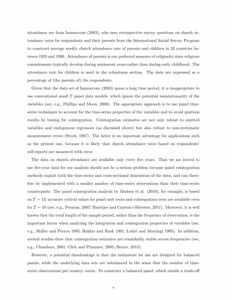
Table 1. Countries and Summary Statistics

Average of CHURCHit Average of log(yit)

Australia 31.85 9.13Austria 50.46 8.75Bulgaria 19.54 7.93Chile 42.38 8.33Denmark 12.08 9.12France 31.31 8.93Germany 26.65 8.94Ireland 94.54 8.50Italy 60.69 8.71Japan 7.77 8.49Netherlands 53.23 9.02New Zealand 31.31 9.11Norway 15.00 8.94Spain 53.85 8.36Sweden 13.08 9.10UK 26.38 9.11United States 55.92 9.38

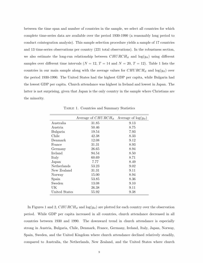
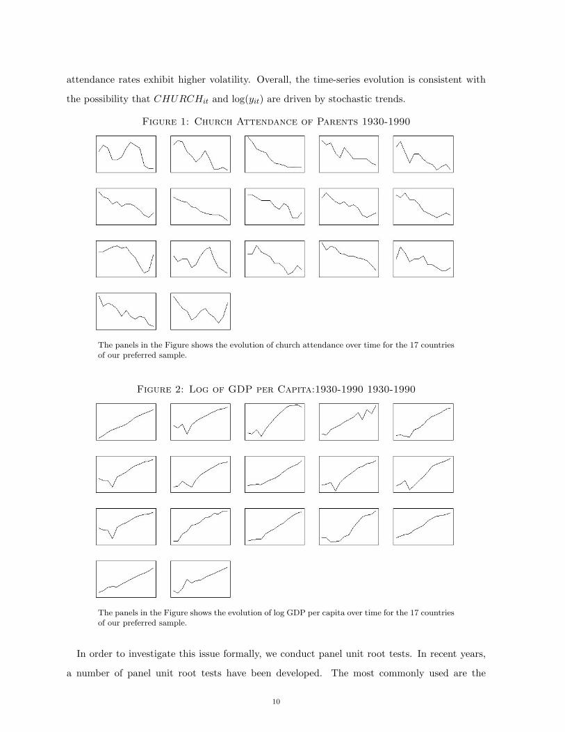
In Figures 1 and 2, CHURCHit and log(yit) are plotted for each country over the observation

period. While GDP per capita increased in all countries, church attendance decreased in all

countries between 1930 and 1990. The downward trend in church attendance is especially

strong in Austria, Bulgaria, Chile, Denmark, France, Germany, Ireland, Italy, Japan, Norway,

Spain, Sweden, and the United Kingdom where church attendance declined relatively steadily,

compared to Australia, the Netherlands, New Zealand, and the United States where church

9

attendance rates exhibit higher volatility. Overall, the time-series evolution is consistent with

the possibility that CHURCHit and log(yit) are driven by stochastic trends.

Figure 1: Church Attendance of Parents 1930-1990

The panels in the Figure shows the evolution of church attendance over time for the 17 countriesof our preferred sample.

Figure 2: Log of GDP per Capita:1930-1990 1930-1990

The panels in the Figure shows the evolution of log GDP per capita over time for the 17 countriesof our preferred sample.

In order to investigate this issue formally, we conduct panel unit root tests. In recent years,

a number of panel unit root tests have been developed. The most commonly used are the

10

so-called first generation panel unit root tests, such as the ADF-Fisher-type test of Madalla

and Wu (1999) (MW), the Breitung (2000) test, the Levin et al. (2002) test, and the Im et

al. (2003) test. Hlouskova and Wagner (2006) find that the Breitung panel unit root test

generally has the highest power and smallest size distortions of any of the first-generation panel

unit root tests. Therefore, we use the Breitung test. Given, however, that the first-generation

tests, which assume cross-sectional independence, exhibit severe size distortions in the presence

of cross-sectional dependence, we also use second-generation panel unit root tests to allow for

cross-sectional dependence. More specifically, we use the panel unit root tests developed by

Breitung and Das (2005) and Pesaran (2007). The Breitung and Das test is an extension of

the Breitung test and is based on modified standard errors that are robust to cross-sectional

dependence. A potential disadvantage of the cross-sectionally robust test is that it requires that

N < T , which prevents us from using our main sample (with N = 17 and T = 13). Therefore,

we apply the Breitung-Das procedure to an alternative sample of 12 countries over 14 time

periods (a sample that also will be used in the robustness section), while the Pesaran panel unit

root test is again applied to the main sample. Like the Breitung test and the Breitung-Das

test, the Pesaran test is an ADF type test. It is based on an average of the individual country

ADF t-statistics and filters out the cross-sectional dependence by augmenting the individual

ADF regressions with the cross-sectional averages of lagged levels and first differences of the

individual series.

As can be seen from Table 2, both the Breitung and the Breitung and Das tests fail to reject

the null hypothesis of a unit root at the 10% level for both variables. The Pesaran test does

not reject the unit root null hypothesis for CHURCHit at the 10% level, while the unit root

null for log(yit) is rejected at the 5% level but not at the 1% level. Given that existing panel

studies usually conclude that real GDP per capita contains a unit root (see, e.g., Pedroni, 2007;

Herzer, et al., 2012), it is reasonable to assume that both CHURCHit and log(yit) are driven

by stochastic trends.

In order to ensure that the relationship between CHURCHit and log(yit) is not spurious,

we test for cointegration using the standard panel and group ADF and PP test statistics sug-

gested by Pedroni (1999, 2004). However, these tests do not take account of potential error

from cross-sectional dependence, which could bias the results. To test for cointegration in the

11

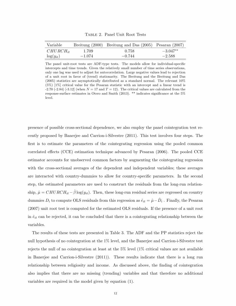
Table 2. Panel Unit Root Tests

Variable Breitung (2000) Breitung and Das (2005) Pesaran (2007)

CHURCHit 1.709 0.758 −3.047∗∗

log(yit) −1.074 −0.744 −2.588

The panel unit-root tests are ADF-type tests. The models allow for individual-specificintercepts and time trends. Given the relatively small number of time series observations,only one lag was used to adjust for autocorrelation. Large negative values lead to rejectionof a unit root in favor of (trend) stationarity. The Breitung and the Breitung and Das(2005) statistics are asymptotically distributed as a standard normal. The relevant 10%(5%) [1%] critical value for the Pesaran statistic with an intercept and a linear trend is-2.70 (-2.84) [-3.12] (when N = 17 and T = 12). The critical values are calculated from theresponse-surface estimates in Otero and Smith (2013). ** indicates significance at the 5%level.

presence of possible cross-sectional dependence, we also employ the panel cointegration test re-

cently proposed by Banerjee and Carrion-i-Silvestre (2011). This test involves four steps. The

first is to estimate the parameters of the cointegrating regression using the pooled common

correlated effects (CCE) estimation technique advanced by Pesaran (2006). The pooled CCE

estimator accounts for unobserved common factors by augmenting the cointegrating regression

with the cross-sectional averages of the dependent and independent variables; these averages

are interacted with country-dummies to allow for country-specific parameters. In the second

step, the estimated parameters are used to construct the residuals from the long-run relation-

ship, µ = CHURCHit− β log(yit). Then, these long-run residual series are regressed on country

dummies Di to compute OLS residuals from this regression as eit = µ−Di . Finally, the Pesaran

(2007) unit root test is computed for the estimated OLS residuals. If the presence of a unit root

in eit can be rejected, it can be concluded that there is a cointegrating relationship between the

variables.

The results of these tests are presented in Table 3. The ADF and the PP statistics reject the

null hypothesis of no cointegration at the 1% level, and the Banerjee and Carrion-i-Silvestre test

rejects the null of no cointegration at least at the 5% level (1% critical values are not available

in Banerjee and Carrion-i-Silvestre (2011)). These results indicate that there is a long run

relationship between religiosity and income. As discussed above, the finding of cointegration

also implies that there are no missing (trending) variables and that therefore no additional

variables are required in the model given by equation (1).

12

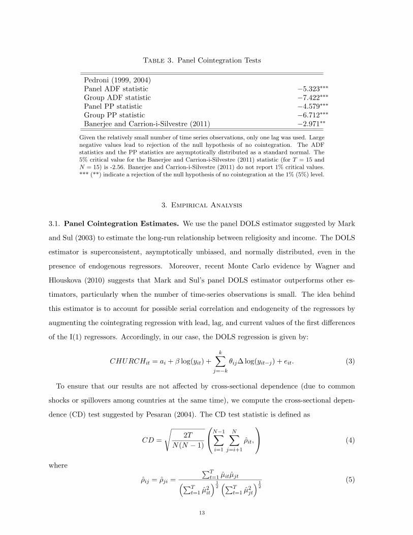
Table 3. Panel Cointegration Tests

Pedroni (1999, 2004)Panel ADF statistic −5.323∗∗∗

Group ADF statistic −7.422∗∗∗

Panel PP statistic −4.579∗∗∗

Group PP statistic −6.712∗∗∗

Banerjee and Carrion-i-Silvestre (2011) −2.971∗∗

Given the relatively small number of time series observations, only one lag was used. Largenegative values lead to rejection of the null hypothesis of no cointegration. The ADFstatistics and the PP statistics are asymptotically distributed as a standard normal. The5% critical value for the Banerjee and Carrion-i-Silvestre (2011) statistic (for T = 15 andN = 15) is -2.56. Banerjee and Carrion-i-Silvestre (2011) do not report 1% critical values.*** (**) indicate a rejection of the null hypothesis of no cointegration at the 1% (5%) level.

3. Empirical Analysis

3.1. Panel Cointegration Estimates. We use the panel DOLS estimator suggested by Mark

and Sul (2003) to estimate the long-run relationship between religiosity and income. The DOLS

estimator is superconsistent, asymptotically unbiased, and normally distributed, even in the

presence of endogenous regressors. Moreover, recent Monte Carlo evidence by Wagner and

Hlouskova (2010) suggests that Mark and Sul’s panel DOLS estimator outperforms other es-

timators, particularly when the number of time-series observations is small. The idea behind

this estimator is to account for possible serial correlation and endogeneity of the regressors by

augmenting the cointegrating regression with lead, lag, and current values of the first differences

of the I(1) regressors. Accordingly, in our case, the DOLS regression is given by:

CHURCHit = ai + β log(yit) +

k∑

j=−k

θij∆ log(yit−j) + eit. (3)

To ensure that our results are not affected by cross-sectional dependence (due to common

shocks or spillovers among countries at the same time), we compute the cross-sectional depen-

dence (CD) test suggested by Pesaran (2004). The CD test statistic is defined as

CD =

√

2T

N(N − 1)

N−1∑

i=1

N∑

j=i+1

ρit,

(4)

where

ρij = ρji =

∑Tt=1 µitµjt

(

∑Tt=1 µ

2it

) 1

2

(

∑Tt=1 µ

2jt

) 1

2

(5)

13

is the sample estimate of the pair-wise correlation of the residuals of the estimated models, µit.

The CD test statistic is normally distributed under the null hypothesis of no cross-sectional

dependence.

As the CD test in the first row of Table 4 shows, the panel DOLS model does not appear

to suffer from cross-sectionally dependent residuals; thus, valid inferences can be drawn from

the regression results. The DOLS regression shows a highly significant negative relationship

between religiosity and income, and the point estimate implies (if viewed causally) that, in the

long run, an increase in per capita GDP by one percent decreases the weekly church attendance

rate by 8.9 percentage points on average in our sample (holding all else constant). Although

this effect seems large, the magnitude is much smaller than that implied by the McCleary and

Barro (2006) estimate.

In the second row of Table 4, we also present DOLS results based on demeaned data. While the

coefficient on the income variable is still negative and significant, it is smaller (in absolute value)

than its counterpart in row 1. However, the CD test indicates the presence of cross sectional

error dependence, which could have biased the results. The finding of cross sectional dependence

for the demeaned data is consistent with studies showing that the demeaning procedure may

introduce cross-sectional correlation among the error terms when it is not already present (see,

e.g., Carporale and Cerrato, 2006). In the following, we therefore use demeaned variables only

when the CD test indicates the presence of cross sectional dependence.

3.2. Robustness. We perform several sensitivity exercises. First, we examine whether the neg-

ative relationship between religiosity and income is robust to alternative estimation techniques.

A potential problem with the pooled results (reported in row 1) could be that they are based on

the implicit assumption of homogeneity of the long-run parameters. It is well known that, while

efficiency gains from the pooling of observations over the cross-sectional units can be achieved

when the individual slope coefficients are the same, pooled estimators may yield inconsistent

and potentially misleading estimates of the sample mean of the individual coefficients when the

true slope coefficients are heterogeneous. Although a comparative study by Baltagi and Grif-

fin (1997) concludes that the efficiency gains from pooling more than offset the biases due to

individual country heterogeneity, we nonetheless allow the long-run coefficients to vary across

countries by using the group-mean panel DOLS estimator suggested by Pedroni (2001). This

estimator involves estimating separate DOLS regressions for each country and averaging the

14

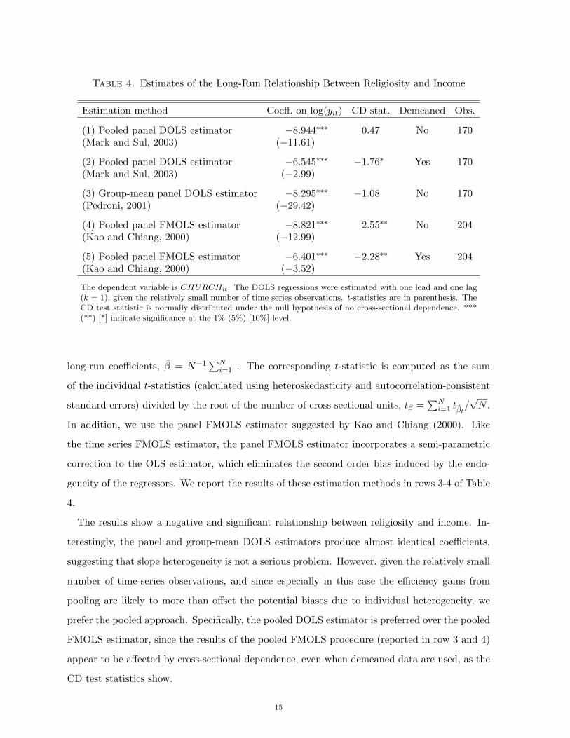
Table 4. Estimates of the Long-Run Relationship Between Religiosity and Income

Estimation method Coeff. on log(yit) CD stat. Demeaned Obs.

(1) Pooled panel DOLS estimator −8.944∗∗∗ 0.47 No 170(Mark and Sul, 2003) (−11.61)

(2) Pooled panel DOLS estimator −6.545∗∗∗ −1.76∗ Yes 170(Mark and Sul, 2003) (−2.99)

(3) Group-mean panel DOLS estimator −8.295∗∗∗ −1.08 No 170(Pedroni, 2001) (−29.42)

(4) Pooled panel FMOLS estimator −8.821∗∗∗ 2.55∗∗ No 204(Kao and Chiang, 2000) (−12.99)

(5) Pooled panel FMOLS estimator −6.401∗∗∗ −2.28∗∗ Yes 204(Kao and Chiang, 2000) (−3.52)

The dependent variable is CHURCHit. The DOLS regressions were estimated with one lead and one lag(k = 1), given the relatively small number of time series observations. t-statistics are in parenthesis. TheCD test statistic is normally distributed under the null hypothesis of no cross-sectional dependence. ***(**) [*] indicate significance at the 1% (5%) [10%] level.

long-run coefficients, β = N−1∑N

i=1 . The corresponding t-statistic is computed as the sum

of the individual t-statistics (calculated using heteroskedasticity and autocorrelation-consistent

standard errors) divided by the root of the number of cross-sectional units, tβ =∑N

i=1 tβt/√N .

In addition, we use the panel FMOLS estimator suggested by Kao and Chiang (2000). Like

the time series FMOLS estimator, the panel FMOLS estimator incorporates a semi-parametric

correction to the OLS estimator, which eliminates the second order bias induced by the endo-

geneity of the regressors. We report the results of these estimation methods in rows 3-4 of Table

4.

The results show a negative and significant relationship between religiosity and income. In-

terestingly, the panel and group-mean DOLS estimators produce almost identical coefficients,

suggesting that slope heterogeneity is not a serious problem. However, given the relatively small

number of time-series observations, and since especially in this case the efficiency gains from

pooling are likely to more than offset the potential biases due to individual heterogeneity, we

prefer the pooled approach. Specifically, the pooled DOLS estimator is preferred over the pooled

FMOLS estimator, since the results of the pooled FMOLS procedure (reported in row 3 and 4)

appear to be affected by cross-sectional dependence, even when demeaned data are used, as the

CD test statistics show.

15

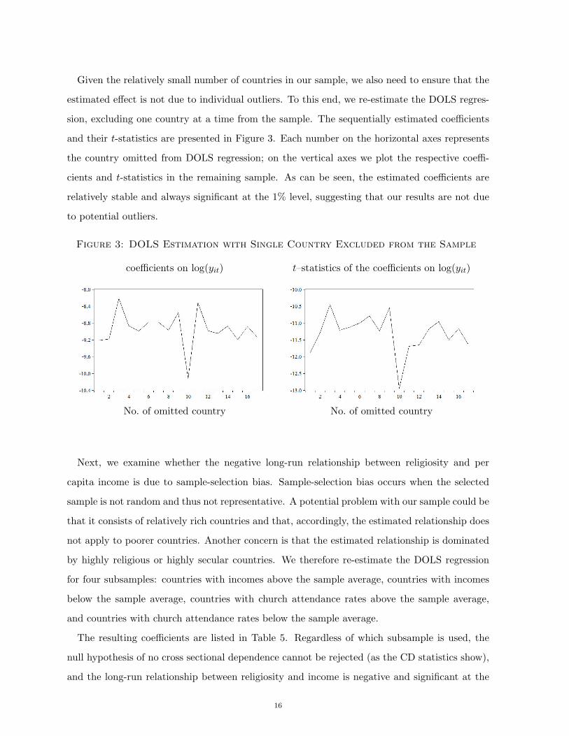
Given the relatively small number of countries in our sample, we also need to ensure that the

estimated effect is not due to individual outliers. To this end, we re-estimate the DOLS regres-

sion, excluding one country at a time from the sample. The sequentially estimated coefficients

and their t-statistics are presented in Figure 3. Each number on the horizontal axes represents

the country omitted from DOLS regression; on the vertical axes we plot the respective coeffi-

cients and t-statistics in the remaining sample. As can be seen, the estimated coefficients are

relatively stable and always significant at the 1% level, suggesting that our results are not due

to potential outliers.

Figure 3: DOLS Estimation with Single Country Excluded from the Sample

coefficients on log(yit) t–statistics of the coefficients on log(yit)

No. of omitted country No. of omitted country

Next, we examine whether the negative long-run relationship between religiosity and per

capita income is due to sample-selection bias. Sample-selection bias occurs when the selected

sample is not random and thus not representative. A potential problem with our sample could be

that it consists of relatively rich countries and that, accordingly, the estimated relationship does

not apply to poorer countries. Another concern is that the estimated relationship is dominated

by highly religious or highly secular countries. We therefore re-estimate the DOLS regression

for four subsamples: countries with incomes above the sample average, countries with incomes

below the sample average, countries with church attendance rates above the sample average,

and countries with church attendance rates below the sample average.

The resulting coefficients are listed in Table 5. Regardless of which subsample is used, the

null hypothesis of no cross sectional dependence cannot be rejected (as the CD statistics show),

and the long-run relationship between religiosity and income is negative and significant at the

16

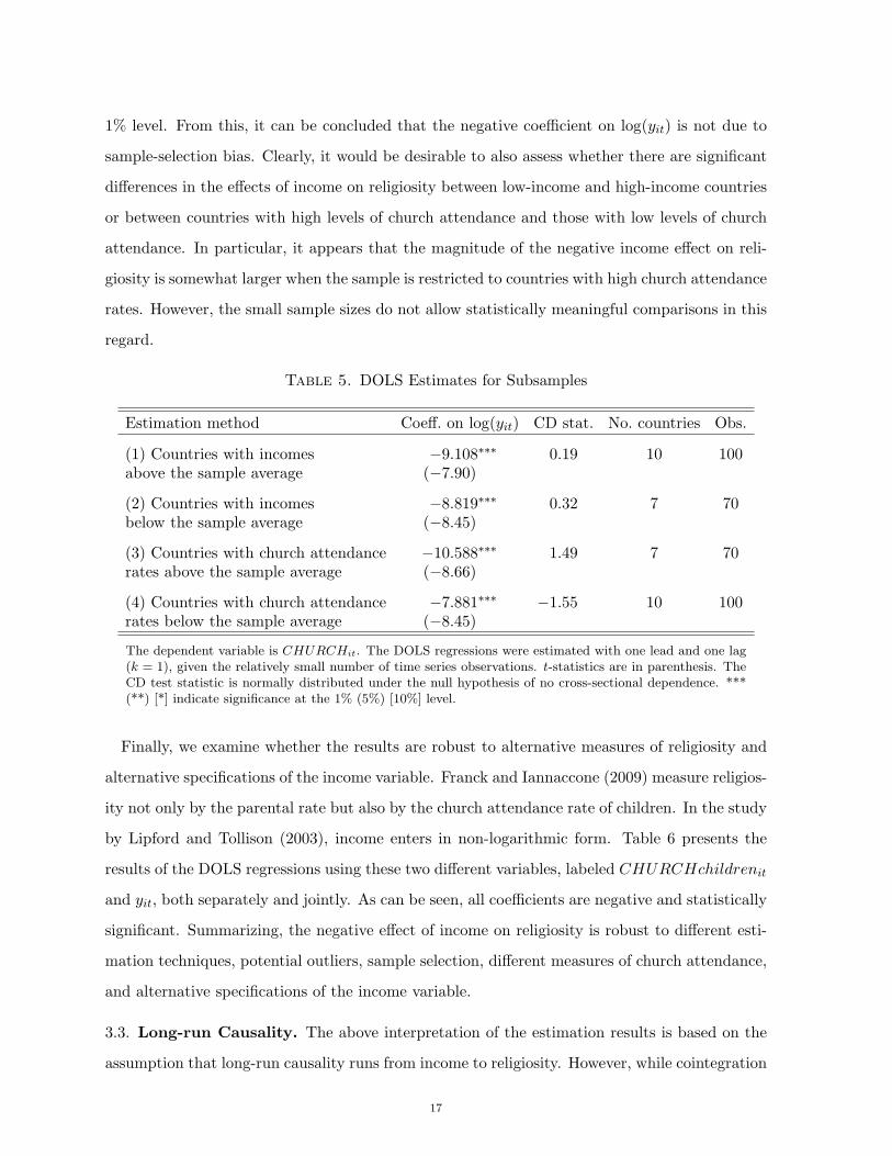
1% level. From this, it can be concluded that the negative coefficient on log(yit) is not due to

sample-selection bias. Clearly, it would be desirable to also assess whether there are significant

differences in the effects of income on religiosity between low-income and high-income countries

or between countries with high levels of church attendance and those with low levels of church

attendance. In particular, it appears that the magnitude of the negative income effect on reli-

giosity is somewhat larger when the sample is restricted to countries with high church attendance

rates. However, the small sample sizes do not allow statistically meaningful comparisons in this

regard.

Table 5. DOLS Estimates for Subsamples

Estimation method Coeff. on log(yit) CD stat. No. countries Obs.

(1) Countries with incomes −9.108∗∗∗ 0.19 10 100above the sample average (−7.90)

(2) Countries with incomes −8.819∗∗∗ 0.32 7 70below the sample average (−8.45)

(3) Countries with church attendance −10.588∗∗∗ 1.49 7 70rates above the sample average (−8.66)

(4) Countries with church attendance −7.881∗∗∗ −1.55 10 100rates below the sample average (−8.45)

The dependent variable is CHURCHit. The DOLS regressions were estimated with one lead and one lag(k = 1), given the relatively small number of time series observations. t-statistics are in parenthesis. TheCD test statistic is normally distributed under the null hypothesis of no cross-sectional dependence. ***(**) [*] indicate significance at the 1% (5%) [10%] level.

Finally, we examine whether the results are robust to alternative measures of religiosity and

alternative specifications of the income variable. Franck and Iannaccone (2009) measure religios-

ity not only by the parental rate but also by the church attendance rate of children. In the study

by Lipford and Tollison (2003), income enters in non-logarithmic form. Table 6 presents the

results of the DOLS regressions using these two different variables, labeled CHURCHchildrenit

and yit, both separately and jointly. As can be seen, all coefficients are negative and statistically

significant. Summarizing, the negative effect of income on religiosity is robust to different esti-

mation techniques, potential outliers, sample selection, different measures of church attendance,

and alternative specifications of the income variable.

3.3. Long-run Causality. The above interpretation of the estimation results is based on the

assumption that long-run causality runs from income to religiosity. However, while cointegration

17

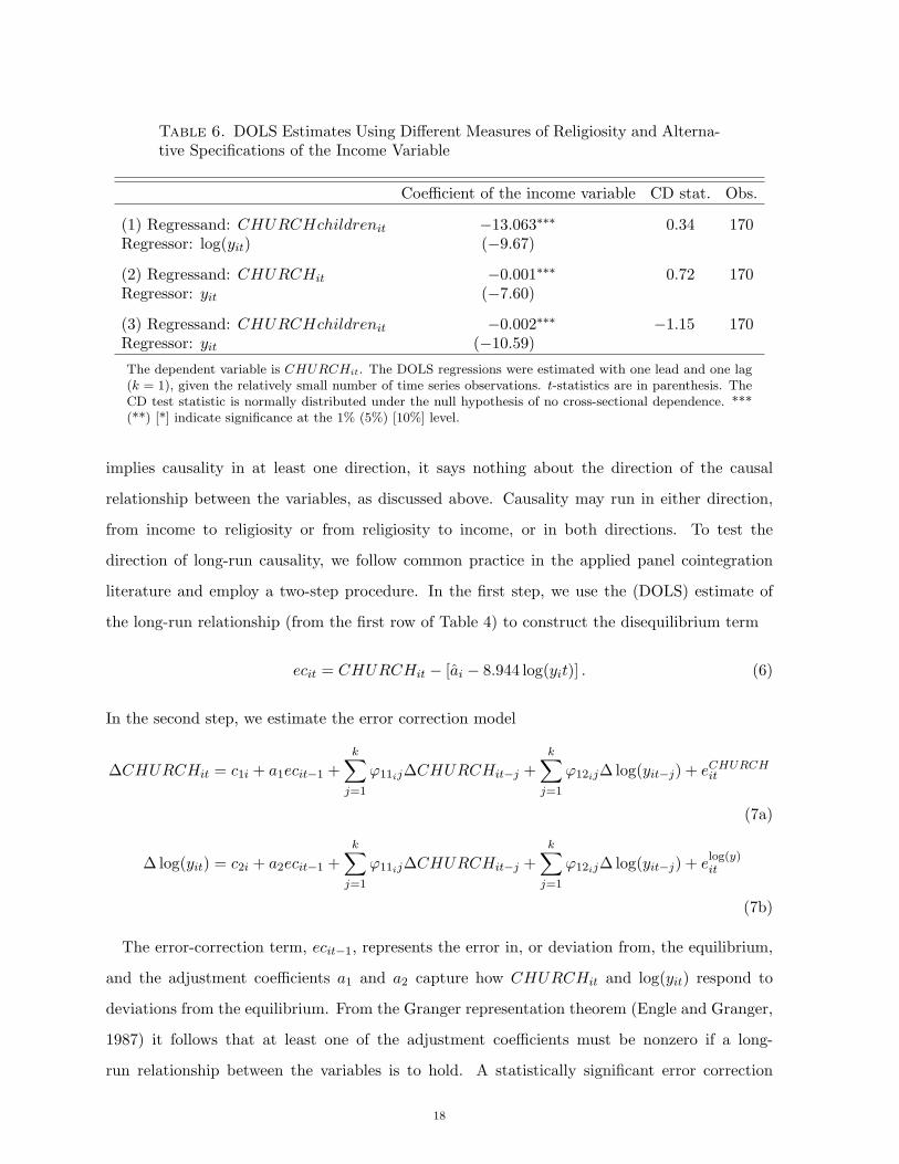
Table 6. DOLS Estimates Using Different Measures of Religiosity and Alterna-tive Specifications of the Income Variable

Coefficient of the income variable CD stat. Obs.

(1) Regressand: CHURCHchildrenit −13.063∗∗∗ 0.34 170Regressor: log(yit) (−9.67)

(2) Regressand: CHURCHit −0.001∗∗∗ 0.72 170Regressor: yit (−7.60)

(3) Regressand: CHURCHchildrenit −0.002∗∗∗ −1.15 170Regressor: yit (−10.59)

The dependent variable is CHURCHit. The DOLS regressions were estimated with one lead and one lag(k = 1), given the relatively small number of time series observations. t-statistics are in parenthesis. TheCD test statistic is normally distributed under the null hypothesis of no cross-sectional dependence. ***(**) [*] indicate significance at the 1% (5%) [10%] level.

implies causality in at least one direction, it says nothing about the direction of the causal

relationship between the variables, as discussed above. Causality may run in either direction,

from income to religiosity or from religiosity to income, or in both directions. To test the

direction of long-run causality, we follow common practice in the applied panel cointegration

literature and employ a two-step procedure. In the first step, we use the (DOLS) estimate of

the long-run relationship (from the first row of Table 4) to construct the disequilibrium term

ecit = CHURCHit − [ai − 8.944 log(yit)] . (6)

In the second step, we estimate the error correction model

∆CHURCHit = c1i + a1ecit−1 +

k∑

j=1

ϕ11ij∆CHURCHit−j +

k∑

j=1

ϕ12ij∆ log(yit−j) + eCHURCHit

(7a)

∆ log(yit) = c2i + a2ecit−1 +k

∑

j=1

ϕ11ij∆CHURCHit−j +k

∑

j=1

ϕ12ij∆ log(yit−j) + elog(y)it

(7b)

The error-correction term, ecit−1, represents the error in, or deviation from, the equilibrium,

and the adjustment coefficients a1 and a2 capture how CHURCHit and log(yit) respond to

deviations from the equilibrium. From the Granger representation theorem (Engle and Granger,

1987) it follows that at least one of the adjustment coefficients must be nonzero if a long-

run relationship between the variables is to hold. A statistically significant error correction

18

term also implies long-run Granger causality from the explanatory variables to the dependent

variables (Granger, 1988), and thus that the dependent variables are endogenous in the long

run. An insignificant error correction term implies long-run Granger non-causality, and thus that

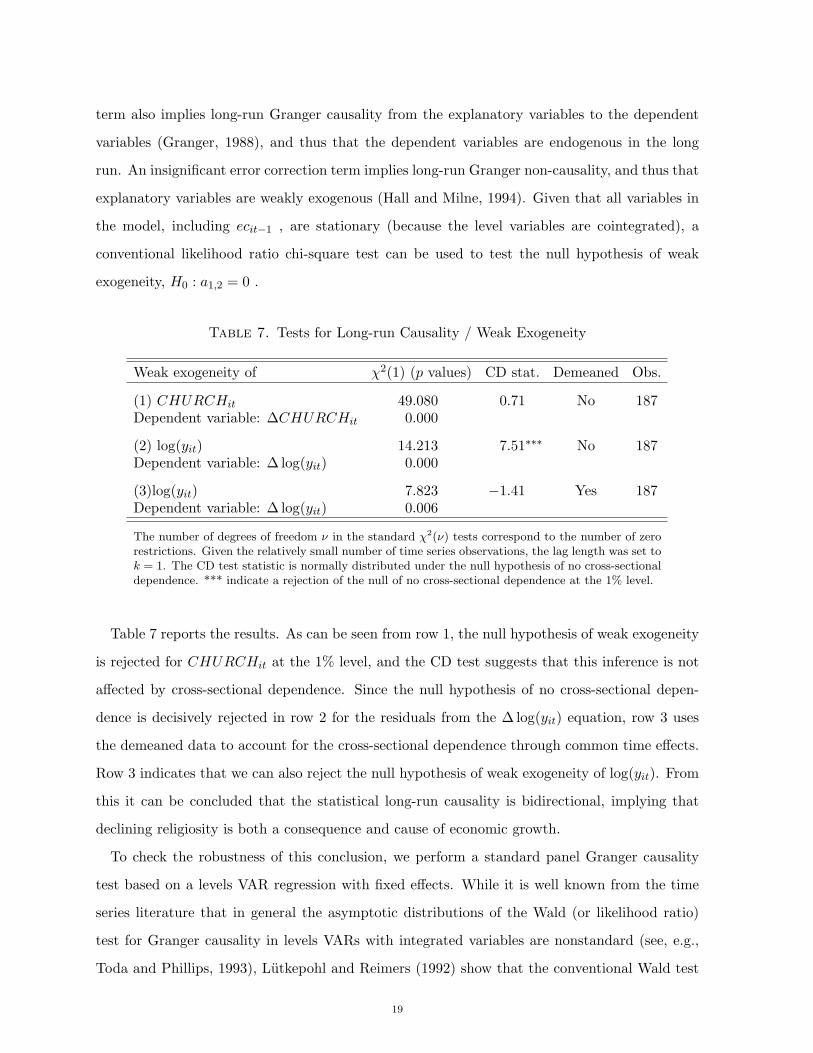
explanatory variables are weakly exogenous (Hall and Milne, 1994). Given that all variables in

the model, including ecit−1 , are stationary (because the level variables are cointegrated), a

conventional likelihood ratio chi-square test can be used to test the null hypothesis of weak

exogeneity, H0 : a1,2 = 0 .

Table 7. Tests for Long-run Causality / Weak Exogeneity

Weak exogeneity of χ2(1) (p values) CD stat. Demeaned Obs.

(1) CHURCHit 49.080 0.71 No 187Dependent variable: ∆CHURCHit 0.000

(2) log(yit) 14.213 7.51∗∗∗ No 187Dependent variable: ∆ log(yit) 0.000

(3)log(yit) 7.823 −1.41 Yes 187Dependent variable: ∆ log(yit) 0.006

The number of degrees of freedom ν in the standard χ2(ν) tests correspond to the number of zerorestrictions. Given the relatively small number of time series observations, the lag length was set tok = 1. The CD test statistic is normally distributed under the null hypothesis of no cross-sectionaldependence. *** indicate a rejection of the null of no cross-sectional dependence at the 1% level.

Table 7 reports the results. As can be seen from row 1, the null hypothesis of weak exogeneity

is rejected for CHURCHit at the 1% level, and the CD test suggests that this inference is not

affected by cross-sectional dependence. Since the null hypothesis of no cross-sectional depen-

dence is decisively rejected in row 2 for the residuals from the ∆ log(yit) equation, row 3 uses

the demeaned data to account for the cross-sectional dependence through common time effects.

Row 3 indicates that we can also reject the null hypothesis of weak exogeneity of log(yit). From

this it can be concluded that the statistical long-run causality is bidirectional, implying that

declining religiosity is both a consequence and cause of economic growth.

To check the robustness of this conclusion, we perform a standard panel Granger causality

test based on a levels VAR regression with fixed effects. While it is well known from the time

series literature that in general the asymptotic distributions of the Wald (or likelihood ratio)

test for Granger causality in levels VARs with integrated variables are nonstandard (see, e.g.,

Toda and Phillips, 1993), Lutkepohl and Reimers (1992) show that the conventional Wald test

19

for a bivariate cointegrated VAR model is asymptotically distributed as chi-square and therefore

valid as a test for Granger causality.

We report the p-values of the Granger causality chi-square statistics using one and two lags,

respectively, of each variable in Table 8. The number of lags was determined by the Schwarz

criterion (with a maximum of two lags), as is common practice in testing for Granger causality

in a VAR model. As can be seen from the first row, the null hypothesis of no Granger causality

from log(yit) to CHURCHit is decisively rejected, and the sum of the coefficients on lagged

income is negative in the church attendance equation. This confirms our result that increasing

income leads to declining religiosity.

Rows 2 and 3 of Table 8 show that the Granger causality test rejects the null hypothesis that

one lag of CHURCHit does not help predict log(yit) at the 1% level and that the coefficient

on lagged church attendance is also negative. While the CD test rejects the null hypothesis

of no cross sectional dependence in row 2, the results in row 3, using the demeaned data, do

not appear to suffer from cross sectional dependence. These results support the conclusion that

increasing religiosity leads to declining income.

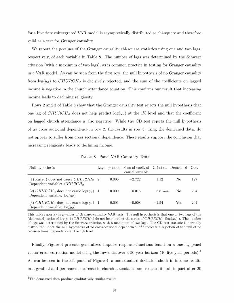
Table 8. Panel VAR Causality Tests

Null hypothesis Lags p-value Sum of coeff. of CD stat. Demeaned Obs.causal variable

(1) log(yit) does not cause CHURCHit 2 0.000 −2.722 1.12 No 187Dependent variable: CHURCHit

(2) CHURCHit does not cause log(yit) 1 0.000 −0.015 8.81∗∗∗ No 204Dependent variable: log(yit)

(3) CHURCHit does not cause log(yit) 1 0.006 −0.008 −1.54 Yes 204Dependent variable: log(yit)

This table reports the p-values of Granger-causality VAR tests. The null hypothesis is that one or two lags of the(demeaned) series of log(yit) (CHURCHit) do not help predict the series of CHURCHit (log(yit) ). The numberof lags was determined by the Schwarz criterion with a maximum of two lags. The CD test statistic is normallydistributed under the null hypothesis of no cross-sectional dependence. *** indicate a rejection of the null of nocross-sectional dependence at the 1% level.

Finally, Figure 4 presents generalized impulse response functions based on a one-lag panel

vector error correction model using the raw data over a 50-year horizon (10 five-year periods).4

As can be seen in the left panel of Figure 4, a one-standard-deviation shock in income results

in a gradual and permanent decrease in church attendance and reaches its full impact after 20

4The demeaned data produce qualitatively similar results.

20

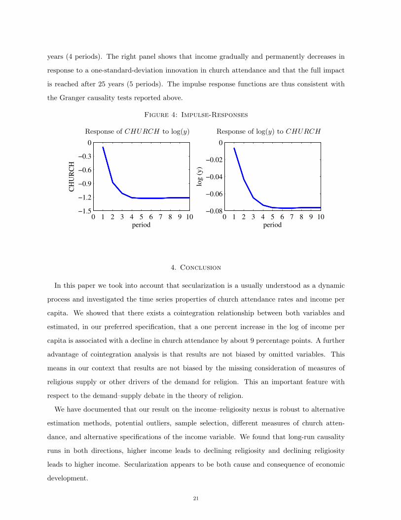
years (4 periods). The right panel shows that income gradually and permanently decreases in

response to a one-standard-deviation innovation in church attendance and that the full impact

is reached after 25 years (5 periods). The impulse response functions are thus consistent with

the Granger causality tests reported above.

Figure 4: Impulse-Responses

Response of CHURCH to log(y) Response of log(y) to CHURCH

0 1 2 3 4 5 6 7 8 9 10−1.5

−1.2

−0.9

−0.6

−0.3

0

period

CH

UR

CH

0 1 2 3 4 5 6 7 8 9 10−0.08

−0.06

−0.04

−0.02

0

period

log (

y)

4. Conclusion

In this paper we took into account that secularization is a usually understood as a dynamic

process and investigated the time series properties of church attendance rates and income per

capita. We showed that there exists a cointegration relationship between both variables and

estimated, in our preferred specification, that a one percent increase in the log of income per

capita is associated with a decline in church attendance by about 9 percentage points. A further

advantage of cointegration analysis is that results are not biased by omitted variables. This

means in our context that results are not biased by the missing consideration of measures of

religious supply or other drivers of the demand for religion. This an important feature with

respect to the demand–supply debate in the theory of religion.

We have documented that our result on the income–religiosity nexus is robust to alternative

estimation methods, potential outliers, sample selection, different measures of church atten-

dance, and alternative specifications of the income variable. We found that long-run causality

runs in both directions, higher income leads to declining religiosity and declining religiosity

leads to higher income. Secularization appears to be both cause and consequence of economic

development.

21

One limitation of our analysis is the relatively small sample of countries, consisting mostly

of developed Western countries primarily inhabited by (former) Christians. Whether and how

the results are transferable to developing countries and countries inhabited predominantly by

non-Christians is an intriguing question, which we are looking forward to address when time

series data on religiosity will be available for these countries as well.

Eventually, with respect to future developments, the strong linear relationship between church

attendance and the log of income has to become non-linear if income continues to grow because

church attendance is bounded from below. Our analysis, comprising most of the 20th century,

however, has shown that a fading trend of secularization is not yet visible in the data.

22

References

Acemoglu, D. (2009). Introduction to Modern Economic Growth. Princeton University Press.

Azzi, C. and Ehrenberg, R. (1975). Household allocation of time and church attendance, Journal

of Political Economy 83, 27-56.

Baltagi, B.H. and Griffin, J.M. (1997). Pooled estimators vs. their heterogeneous counterparts

in the context of dynamic demand for gasoline. Journal of Econometrics 77(2), 303-327.

Banerjee, A. and Carrion-i-Silvestre, J.J. (2011). Testing for panel cointegration using com-

mon correlated effects estimators. Department of Economics Discussion Paper No. 11-16.

University of Birmingham.

Becker, S.O. and Woessmann, L. (2009). Was Weber wrong? A human capital theory of

Protestant economic history. Quarterly Journal of Economics 124 531–596.

Becker, S.O. and Woessmann, L. (2013). Not the opium of the people: Income and secularization

in a panel of Prussian counties. Centre For Economic Policy Discussion Paper No. 9299.

London: London School of Economics.

Bonham, C.S. and Cohen, R. H. (2001). To aggregate, pool, or neither. Testing the rational-

expectations hypothesis using survey data. Journal of Business and Economic Statistics,

19(3) 278-291.

Breitung, J. (2000). The local power of some unit root tests for panel data. Advances in

Econometrics 15, 161-177.

Breitung, J. and Das, S. (2005). Panel unit root tests under cross-sectional dependence. Statis-

tica Neerlandica, 59(4) 414-433.

Bruce, S. (2011). Secularization: In Defence of an Unfashionable Theory. Oxford University

Press.

Caporale, G.M., Cerrato, M. (2006) Panel data tests of PPP: a critical overview. Applied

Financial Economics 16(1-2), 73-91.

Chambers, M.J. (2001). Cointegration and sampling frequency. Department of Economics

Discussion Paper No. 531, University of Essex.

Davidson, J. (1998). Structural relations, cointegration and identification: some simple results

and their application. Journal of Econometrics, 87(1), 87-113.

Dobbelaere, K. (1987) Some trends in the European sociology of religion: the secularization

debate. Sociological Analysis 48, 10737.

Eberhardt, M. and Teal, F. (2013). Structural change and cross-country growth empirics. World

Bank Economic Review, forthcoming.

Engle, R.E. and Granger, C.W.J. (1987). Cointegration and error-correction: representation,

estimation, and testing. Econometrica 55(2), 251-276.

23

Entorf, H. (1997). Random walks with drifts: nonsense regression and spurious fixed-effects

estimation. Journal of Econometrics 80(2), 287-96.

Everaert, G. (2011). Estimation and inference in time series with omitted I(1) variables. Journal

of Time Series Econometrics 2(2), 1-26.

Finke, R. and Innaccone, L.R. (1993). Supply-side explanations for religious change, Annals of

the American Academy of Political and Social Sciences 527, 27-39.

Franck, R., Iannaccone, L.R. (2009). Why did religiosity decrease in the Western World during

the twentieth century? Mimeo, Bar-Ilan University.

Click, R.W. and Plummer, M.G. (2005). Stock market integration in ASEAN after the Asian

financial crisis. Journal of Asian Economics, 16(1) Pages 5-28.

Granger, C.W.J. (1988). Some recent developments in a concept of causality. Journal of Econo-

metrics 39(1-2), 1988, 199-211.

Granger, C.W.J. and Newbold, P. (1974). Spurious regressions in econometrics. Journal of

Econometrics 2(2), 111-120.

Guiso, L., Sapienza, P., and Zingales, L. (2003). People’s opium? Religion and economic

attitudes, Journal of Monetary Economics 50, 225-282.

Hall, S.G. and Milne, A. (1994). The relevance of P-star analysis to UK monetary policy.

Economic Journal 104(424), 597-604.

Hakkio C.S. and Rush, M. (1991). Cointegration: How short is the long run? it Journal of

International Money and Finance 10(4), 571-581.

Herzer, D., Strulik, H., and Vollmer, S., (2012). The long-run determinants of fertility: one

century of demographic change 1900-1999. Journal of Economic Growth 17(4), 357-385.

Herzer, D. (2013). Cross-country heterogeneity and the trade-income relationship. World De-

velopment, 44(4), 194-211.

Hlouskova, L., Wagner, M. (2006). The performance of panel unit root and stationary tests:

results from a large scale simulation study. Econometric Reviews 25(1), 85-116.

Iannaccone, L. (2003). Looking backward: A cross-national study of religious trends. Mimeo,

George Mason University.

Im, K.S., Pesaran, M.H., and Shin, Y. (2003). Testing for unit roots in heterogeneous panels.

Journal of Econometrics 115(1), 53-74.

Juselius, K. (1996). An empirical analysis of the changing role of the German Bundesbank after

1983. Oxford Bulletin of Economics and Statistics 58(4), 791-819.

Juselius, K. (2006). The cointegrated VAR Model: Methodology and Applications. Oxford:

University Press.

24

Kao, C. (1999). Spurious regression and residual-based tests for cointegration in panel data.

Journal of Econometrics 90(1), 1-44.

Kao, C. and Chiang., M., (2000). On the estimation and inference of a cointegrated regression

in panel data. Advances in Econometrics 15, 179-222.

Lahiri, K. and Mamingi, N. (1995). Power versus frequency of observation another view. Eco-

nomics Letters 49(2), 121-124.

Levin, A., Lin, C.-F., and Chu, C.-S.J. (2002). Unit root test in panel data: asymptotic and

finite-sample properties. Journal of Econometrics 108(1), 1-24.

Lipford, J.W. and Tollison, R. D. (2003). Religious participation and income. Journal of

Economic Behavior and Organization 51(2), 249-260.

Lutkepohl, H. (2007). General-to-specific or specific-to-general modelling? An opinion on cur-

rent econometric terminology. Journal of Econometrics 136(1), 319-324.

Lutkepohl, H. and Reimers, H.-E., (1992). Granger-causality in cointegrated VAR processes.

The case of the term structure. Economics Letters 40(3), 263-268.

Madalla, G.S. and Wu, S. (1999). A comparative study of unit root tests with panel data and

a new simple test. Oxford Bulletin of Economics and Statistics 61(Special Issue), 631-652.

Maddison, A. (2003). The World Economy: Historical statistics. OECD, Paris.

Madsen, J.B.,Saxena, S., and Ang, J.B. (2010). The Indian growth miracle and endogenous

growth. Journal of Development Economics 93(1), 37-48.

McCleary, R. M. and Barro, R. J. (2006a). Religion and political economy in an international

panel. Journal for the Scientific Study of Religion 45(2), 149-175.

McCleary, R.M. and Barro, R.J. (2006b). Religion and economy. Journal of Economic Perspec-

tives 20(2), 49-72.

Norris, P. and Inglehart, R. (2004). Sacred and Secular, Cambridge University Press.

Otero, J. and Smith, J. (2013). Response surface estimates of the cross-sectionally augmented

IPS tests for panel unit roots. Computational Economics 41(1), 1-9.

Pedroni, P. (1999). Critical values for cointegration tests in heterogeneous panels with multiple

regressors. Oxford Bulletin of Economics and Statistics 61(Special Issue Nov.), 653-670.

Pedroni, P. (2001). Purchasing power parity tests in cointegrated panels. Review of Economics

and Statistics 83(4), 727-731.

Pedroni, P. (2004). Panel cointegration: Asymptotic and finite sample properties of pooled time

series tests with an application to the PPP hypothesis. Econometric Theory 20(3), 597-625.

Pedroni, P. (2007). Social capital, barriers to production and capital shares: implications for

the importance of parameter heterogeneity from a nonstationary panel approach. Journal of

Applied Econometrics 22(2), 429-451.

25

Pesaran, M.H. (2004). General diagnostic tests for cross section dependence in panels. CESifo

Working Paper Series 1229, CESifo Group Munich.

Pesaran, M.H. (2006). Estimation and inference in large heterogeneous panels with a multifactor

error structure. Econometrica 74(4), 967-1012.

Pesaran, M.H. (2007). A simple panel unit root test in the presence of cross-section dependence.

Journal of Applied Econometrics 22(2), 265-312.

Phillips, P. and Moon, H. (2000). Nonstationary panel data analysis: an overview of some recent

developments. Econometric Reviews 19(3), 263-286.

Shiller, R.J. and Perron, P. (1985). Testing the random walk hypothesis: power versus frequency

of observation. Economics Letters 18(4), 381-386.

Stock, J. H. (1987). Asymptotic properties of least squares estimators of cointegrating vectors.

Econometrica 55(5), 1035-1056.

Strulik, H. (2012). From Worship to Worldly Pleasures: Secularization and Long-Run Economic

Growth, University of Goettingen, CRC Discussion Paper 116.

Toda, H.Y. and Phillips, P.C.B. (1993). Vector autoregressions and causality. Econometrica

61(6), 1367-1393.

Wagner, M. and Hlouskova, J. (2010). The performance of panel cointegration methods: results

from a large scale simulation study. Econometric Reviews 29(2), 182-223.

Voas, D. (2008). The rise and fall of fuzzy fidelity in Europe, European Sociological Review 25,

155-168.

Wilson, B. (2003). Secularisation, in: Slattery, Martin (ed.), Key Ideas in Sociology, Nelson

Thornes Ltd.

26