A Viscous Paint Model for Interactive Applications

William Baxter, Yuanxin Liu and Ming C. LinDepartment of Computer Science

University of North Carolina at Chapel Hill{baxter,liuy,lin}@cs.unc.edu

Abstract: We present a viscous paint model for use in an inter-active painting system based on the well-known Stokes’ equationsfor viscous flow. Our method is, to our knowledge, the first un-conditionally stable numerical method that treats viscous fluid witha free surface boundary. We have also developed a real-time im-plementation of the Kubelka-Munk reflectance model for pigmentmixing, compositing and rendering entirely on graphics hardware,using programmable fragment shading capabilities. We have in-tegrated our paint model with a prototype painting system, whichdemonstrates the model’s effectiveness in rendering viscous paintand capturing a thick,impasto-like style of painting. Several usershave tested our prototype system and were able to start creatingoriginal art work in an intuitive manner not possible with the exist-ing techniques in commercial systems.

1 IntroductionFor centuries, artists have used traditional media and tools to ex-press their thoughts and feelings creatively. Recently there has beena growing interest in non-photorealistic rendering and in simulatingartists’ traditional media and tools.

In painting, each paint medium has its own characteristics. Vis-cous paint media, such as oils and acrylics, are popular amongartists for their versatility and ability to capture a wide range ofexpressive styles. However, it is a challenge to design an interac-tive model that correctly captures the physical behavior of viscouspaint, because of the complex underlying set of partial differentialequations that govern that motion.

With the increasing trend to use simulation techniques to au-tomatically generate physically-based, realistic special effects, themodeling of fluid-like behavior has recently received much atten-tion. Most of this attention, however, has been focused on theanimation of very low-viscosity fluids such as water or air. Butmany fluids that we encounter on a daily basis are of a more vis-cous nature. Familiar examples include honey, glue, mud, ketchup,and thick paints. A method for simulating such media interactivelymust be capable of treating both the high viscosity and the complexfree-surface boundary conditions with unconditional stability.

In addition to focusing on the plausible physical behavior ofviscous paint, we are also aiming at providing an expressive vehiclefor the users tointeractivelycreate original works using computersystems. This set of dual goals introduce strict constraints and newchallenges on the design and implementation of a computationalmodel for a viscous paint medium.Main Contributions: In this paper, we present an interactivemethod for modeling very viscous paint media based on a novelstable solver for the viscous Stokes equations, particularly tailoredfor use in painting simulation. The solver can compute 3D flowthroughout the fluid medium and allows realistic mixing of materialproperties (e.g. pigmentation) internally. It uses a Volume-of-Fluid(VOF) / level set technique to track the free surface and is com-pletely stable based on our observation and user’s experiences. Itfurther supports an intuitive, physically-based interaction paradigmfor emulating traditional painting settings [Baxter et al. 2001].

Our main goal is to create a paint model that simulates and ren-

ders viscous paint, such as oil or acrylic paint, for interactive ap-plications. To more accurately recreate the non-linear chromaticbehavior of real paint blending, we have also implemented colormixing and compositing based on the Kubelka-Munk (K-M) model.In order to achieve real-time performance, this is implemented ingraphics hardware using programmable fragment shading capabili-ties. This approach allows for both real-time calculation of the K-Mreflectances and dynamic lighting of the paint surface which wouldotherwise be difficult to attain on a desktop PC.

We have augmented a prototype painting system, which demon-strates the capabilities of our viscous paint medium with real-timeKubelka-Munk mixing and compositing, and several users havecreated paintings using the system. By manipulating the virtualbrush naturally the user can build up layers of paint and paintings ina thick, impasto style. The multiple layers are then rendered usingK-M optical composition on graphics hardware. Together with thephysically-based modeling of the 3D deformable brushes, our vis-cous paint model allows the artists to express their creativity freelyand paint naturally through a more familiar 3D painting interfacethan the typical 2D mouse and widgets.Organization: The rest of the paper is organized as follows.We provide a brief survey of related work in Sec. 2. We presentan overview of the interactive painting system and the user in-terface in Sec. 3. We describe our method for modeling viscousfluid in Sec. 4. Section 5 presents our real-time implementation ofKubelka-Munk model using graphics hardware. We discuss the im-plementation issues and demonstrate the performance of our modelin Sec. 6.

2 Previous WorkA number of researchers have investigated paint and fluid simu-lation, and also paint rendering. We present a brief summary ofrelated work below.

2.1 Fluid and Paint Simulation

[Kass and Miller 1990] used the linearized shallow-water equationsto simulate surface waves. The method is fast, stable and interac-tive, but cannot handle viscous flow, and only simulates the surfaceheight. Internal flow is not computed. [O’Brien and Hodgins 1995]combined a particle system with shallow-water equations to simu-late splashing of low viscosity fluid.

[Chen and Lobo 1995] used 2D Navier-Stokes equations, takingthe pressure to be proportional to height to get the third dimension.The method is interactive though the physical justification for inter-preting pressure as height is questionable. Also, since the methodis fundamentally 2D, the internal flow and mixing are unknown.

[Foster and Metaxas 1996] used an explicit marker-and-cell(MAC) method based on [Harlow and Welch 1965] to simulatelow viscosity free-surface liquid. Being an explicit method, itwas subject to the so-called CFL and viscosity timestep restrictions(∆t < O(∆x), and∆t < O(∆x2), respectively), making it un-suitable for use in interactive applications.

[Stam 1999] introduced the first unconditionally stable solverfor the Navier-Stokes equations to the graphics community. The

Figure 1:System Architecture

solver’s use of implicit backwards-Euler integration for viscosityallows for high viscosity fluids, but the method does not addressthe complications or stability issues introduced by the presence ofa free surface boundary condition.

Recently, [Foster and Fedkiw 2001; Enright et al. 2002] pre-sented convincingly accurate particle level set methods for low-viscosity free surface flow, but these methods are quite computa-tionally intensive, requiring minutes per frame for simulation.

[Carlson et al. 2002] presented simulations of melting and flow-ing of high-viscosity fluids based on the MAC method. While theirmethod treats viscosity implicitly, advection is still performed ex-plicitly, making it subject to the CFL timestep restriction. Also theirmethod for handling the free surface boundary conditions is notclear and likely subject to a timestep restriction. [X. Wei and Kauf-man 2003] and [Cockshott et al. 1992] present cellular-automatamodels for viscous fluid and paint, respectively, which are inter-active, but neither is based on the actual physical equations thatdescribe viscous fluid.

[Curtis et al. 1997] used a form of the shallow water equationsin their watercolor simulation. Their explicit formulation is subjectto timestep restrictions and is inappropriate for very viscous or verythick layers of fluid.

2.2 Paint RenderingAlvy Ray Smith’s original “Paint” program [Smith 1978] perhapsoffered one of the first 2D methods for simulating the look of paint-ing. A paint rendering model that offers the look of thick, viscouspaint with bump-mapping can be found in [Cockshott et al. 1992].

[Kubelka and Munk 1931; Kubelka 1948; Kubelka 1954] pre-sented the Kubelka-Munk (K-M) equations to accurately approxi-mate the diffuse reflectance of pigmented materials like paint givendescriptions of their constituent pigments and their concentrations.

In computer graphics, [Hasse and Meyer 1992] demonstratedthe utility of the K-M equations for rendering and color mixing inboth interactive and offline applications, including a simple “air-brush” painting tool. [Dorsey and Hanrahan 1996] used K-M layercompositing to accurately model the appearance metallic patinas.[Curtis et al. 1997] also used the K-M equations for optically com-positing thin glazes of paint in their watercolor simulation. Noneof these implementations offers the real-time rendering desired forinteractive applications.

3 OverviewIn this section we give a brief overview of our painting system andits user interface design.

3.1 System ArchitectureIn order to test the effectiveness of our viscous paint model, wehave created an enhanced interactive painting system based on ourprevious prototype called dAb [Baxter et al. 2001]. Unlike the ear-lier prototype system, the new dAb system allows the user to choosebetween a haptic stylus or a tablet interface, either of which servesas a physical metaphor for the virtual brush. The brush head ismodeled with a spring-mass particle system skeleton and a subdi-vision surface. It deforms as expected upon contact with the virtualcanvas. A wide selection of common brush types is made availableto the artist.

Our novel viscous paint medium supports important new fea-tures, such as impasto-like strokes and the ability to build up manylayers of paint, both wet and dry, gouging effects from brush marks,per-pixel lighting effects, rendering of paint bumps, etc. The sur-faces of the brush, palette, and canvas are coated with paint usingthis model. A schematic diagram illustrating how various systemcomponents are integrated is shown in Fig. 1.

Figure 2: A Prototype Painting System UsingPHaNTOMTM

with the Graphical User Interface, the Virtual Canvas and theBrush Rack.

Figure 3:The Physical System Setup with a Tablet Interface.

3.2 User InterfaceOur prototype paint system runs on a dual-processor PC equippedwith NVIDIA’s GeForceFX graphics card. One processor is usedfor optional force display, while the other is dedicated to computethe brush dynamics and paint transfer. The color pigment mixing,composition and rendering takes place on the graphics hardware.

A Viscous Paint Model for Interactive Applications 2

Fig. 2 and Fig. 3 show the physical setup of our system with boththe haptic and tablet interfaces.

Unlike the previous dAb system, our new prototype system caninfer the user’s intention from the current user’s hand position. Forexample, as the user moves the brush handle over the brush rackand hovers over a particular brush type, a new brush is automati-cally selected without the user explicitly pressing on the stylus but-ton. As the brush moves over to the virtual palette, the palette isautomatical brought to the center of the screen to allow color pick-ing and paint mixing. The user no longer needs to explicitly togglethe space bar to bring it up.

We also add the ability for having unlimited numbers of undo’sand redo’s, in addition to varying degree of quick drying, savingand loading a clean or previously painted canvas. The implementa-tion of undos differs from our previous dAb system, since the cur-rent paint model allows multiple wet layers, instead of two layers,of paint. This introduces much richer and more complex opticaleffects not available with the existing paint systems.

4 Interactive Paint SimulationIn this section, we describe a physically-based paint model basedon interactive, stable viscous fluid simulation. Our numerical solverfor fluid simulation offers the following characteristics:

• Stable implicit viscosity solver;

• Hybrid linear system solver combines incomplete Choleskypreconditioned conjugate gradient (PCG) with successiveover-relaxation (SOR).

• Stable, semi-Lagrangian update of surface and color;

• Stable treatment of the free-stress surface boundary condi-tions;

We simulate the viscous fluid behavior using the 3D incom-pressible Stokes equations:

∂u

∂t= ν∇2u−∇p+ F (1)

whereu is the velocity of the fluid,ν the kinematic viscosity, andpis the pressure.F represents externally applied forces. We assumeconstant density, since most familiar viscous materials are homo-geneous. Equation 1 is coupled with the equation of continuity,

∇ · u = 0, (2)

which enforces incompressibility and the conservation of mass.The Stokes equation is a simplification of Navier-Stokes applicablefor highly viscous flows. The simplification arises from the obser-vation that the contribution of the advection term which appears inNavier-Stokes,(u · ∇)u, is negligible for viscous fluids with lowReynolds number flows. This can be understood as the velocityfield diffusing so rapidly throughout the fluid that the fluid’s inertiadoes not have time to exert influence on the flow.

4.1 Numerical MethodWe use a standard staggered 3D grid as in [Harlow and Welch 1965;Foster and Metaxas 1996; Griebel et al. 1990] and others, with thevector components such as velocity stored on cell edges and scalarquantities (including color channels) stored at cell centers.

The numerical method used to solve the fluid flow equations isan operator splitting method like many previous, e.g. [Foster andMetaxas 1996; Stam 1999; Carlson et al. 2002]. We first computea provisional velocity field,u∗, that captures the effect of the vis-cous term,ν∇2u, and any externally applied body forces,F. Thisstep uses a stable backwards-Euler integration step. We then solve

a Poisson problem to find a pressure field,p, that will makeu∗ dis-cretely satisfy the compressibility constraint, Eq. 2. Once obtained,the new pressure,p, is used to compute the final divergence-freevelocity field,u.

The above three-step temporal discretization scheme can bewritten succinctly as follows:

u∗ = un + ∆t[ν∇2u∗ + F] (3)

∇2p = ∇ · u∗/∆t (4)

un+1 := u∗ −∆t∇p (5)

wheren refers to the time step at which the variables are to beevaluated.

We model forces applied by the user using boundary conditionsrather than the forcing term,F, and choose to model a fluid viscousenough that gravity is not a significant influence. Thus, we typicallysetF to zero. For less viscous fluid where advection is important,the first step (Eq. 3 can be preceded by a velocity self-advectionstep as in [Stam 1999].

To model and track the evolution of the free surface – the inter-face between the fluid and air – we use a Volume-of-Fluid (VOF)method [Hirt and Nichols 1981] in which every cell in the computa-tional domain is assigned a scalar value between 0 and 1 denotingthe fraction of the cell which is fluid. For the purpose of placingboundary conditions on the simulation, a cell is treated as fluid ifits VOF value is greater than one half. The precise location of thesurface is taken to be thevof = 0.5 isosurface, though this is usedonly for rendering. The method for extracting the isosurface is dis-cussed in Sec. 4.6. Unlike previous free surface methods, each stepof our numerical method is stable, allowing us to take large timesteps and maintain interactivity.

4.2 ViscosityAs can be seen from Eq.3, we solve for the effect of viscosity us-ing an implicit Euler update, which is unconditionally stable [Stam1999; Carlson et al. 2002]. The spatial discretization of Eq. 3 leadsto a system of equations,Ku∗ = un,whereK = I− ν∆t∇2

D and∇2

D is the standard 7-point Laplacian stencil in matrix form. Thesystem is actually three independent systems of equations, one foreach velocity component,u∗, v∗, andw∗. Expanding the compactmatrix notation above out into its constituent linear equations, thesystem of equations for theu∗ component is:

Kcu∗i,j,k +Kx(u∗i−1,j,k + u∗i+1,j,k)

+Ky(u∗i,j−1,k + u∗i,j+1,k)+Kz(u

∗i,j,k−1 + u∗i,j,k+1) = uni,j,k

(6)

where

Kc = 1 + 2ν∆t(1/∆y2 + 1/∆x2 + 1/∆z2)Kx = −ν∆t/∆x2

Ky = −ν∆t/∆y2

Kz = −ν∆t/∆z2

Written as a matrix,K is aD3 × D3 matrix, whereD is thenumber of samples on each dimension of the 3D grid, but the matrixis very sparse, containing onlyO(D3) non-zero entries, makingit amenable to solution with the conjugate gradient method. Weuse the conjugate gradient method with an incomplete Choleskypreconditioner. Pseudo-code algorithms for the conjugate gradientmethod as well as the preconditioner can be found in [Golub andVan Loan 1983].

The sparse matrix multiplies required by the conjugate gradientsolver can be implemented simply by applying the matrix stencil tothe grid, i.e. evaluating the right hand side of (6), at each(i, j, k)on the domain. For example:

A Viscous Paint Model for Interactive Applications 3

for k = 0 to DEPTHfor j = 0 to HEIGHT

for i = 0 to WIDTHif (i,j,k) in domainthen uout(i,j,k) := K_c * uin(i,j,k)

+ K_x * ( uin(i-1,j,k)+uin(i+1,j,k) )+ K_y * ( uin(i,j-1,k)+uin(i,j+1,k) )+ K_z * ( uin(i,j,k-1)+uin(i,j,k+1) );

would compute the productK ∗ uin. The check in line 4 to see ifthe grid cell is in the domain is used when handling domains withirregular geometry. For the implicit viscosity solver, this check istrue if the cell in question is a fluid cell.

4.3 Pressure SolverGiven the tentative velocity field,u∗, we must find a pressure fieldsuch that the divergence ofu∗ −∆t∇p is near zero by solving thePoisson problem (Eq. 4). For low viscosity flows, inertial forcesdominate (i.e., advection) so there is much temporal coherence inthe velocity field. Consequently, a small number of iterations ofsuccessive overrelaxation (SOR) per timestep is sufficient to yieldrealistic-looking results [Foster and Metaxas 1996]. However, invery viscous flow, momentum spreads out quickly, creating largeaccelerations and low temporal coherence. Thus it is necessary touse more solver iterations to enforce incompressibility as viscosityincreases. After experimenting with several different schemes, wehave found a particularly effective approach to be a combinationof both conjugate gradient (CG) and SOR. Our SOR solver stepsare identical to those in [Foster and Metaxas 1996; Griebel et al.1990]. We use between 10-15 iterations of CG with an incompleteCholesky preconditioner, followed by 3 or 4 iterations of SOR. Theresidual after applying CG tends to have a fair amount of high fre-quency content since CG is a “rougher” [Shewchuk 1994]. A fewiterations of SOR applied after CG is particularly effective sinceSOR acts as a “smoother”. In our tests, the CG/SOR combinationwas quantitatively more effective per CPU second than either tech-nique alone. Comparisons were made by calculating convergenceratios for each technique given the same initial conditions and di-viding the result by the computational time required.

4.4 Boundary ConditionsEach stage of the numerical method must be coupled with appropri-ate boundary conditions. For the diffusion step we use the no-slipDirichlet velocity boundary condition,u = 0, at wall boundaries,and set the free velocities on the fluid-air interface to discretelysatisfy the continuity equation (2). We enforce the boundary con-ditions by setting the value of “ghost cells”, which lie just outsidethe domain. For Dirichlet boundary conditions the ghost values onan edge along the interface are simply set to zero. Values just offthe interface are set so that(ughost + uneighbor)/2 = 0, as shownin Fig. 4. For details on implementing the boundary conditions wehighly recommend [Griebel et al. 1990].

For the pressure Poisson equation, Neumann boundary condi-tions are required,∂p/∂n = 0, wheren is the boundary normal.These are implemented by copying the pressure value just insidethe domain to the ghost cell just outside, before every CG or SORiteration. Thus on the face of a boundary cell in the positivex di-rection we have, for example,(pinside − pghost)/∆x = 0, whichis the finite difference approximation to the above boundary condi-tion.

4.5 InteractionRather than adding forcing terms to the Stokes equations to imple-ment interaction with the fluid, we can achieve greater control ofthe fluid by setting Dirichlet velocity boundary conditions at thefluid surface. The velocities of surface cells adjacent to the brushare simply set to the brush’s velocity. This is similar to the approachused for interaction with smoke in [Fedkiw et al. 2001].

Figure 4:Setting Pressure And Velocity Boundary Conditions.

4.6 Free SurfaceUnlike previous approaches, our method for handling the free sur-face of the fluid is stable even at high viscosity. As noted, werepresent the surface implicitly as the level set of a fluid fractionfunction,f(i, j, k), with the interface defined to lie on thef = 0.5isosurface. Insofar as we define the surface using the level set of animplicit function, this approach is similar to that of [Foster and Fed-kiw 2001; Enright et al. 2002], but the specific implicit functionsused are different.

For rendering, we need to compute an approximation of the iso-surface and its normals. The VOF technique represents the true 3Dstructure of the fluid; however, for use as a paint model a heightfield representation is acceptable, and it is much less costly to ex-tract. We obtain a height field from the VOF values in a straight-forward manner by computing one height value for each column ofcells in the grid. We use a simple linear search to find the upper-most fluid cell then interpolate to estimate the isosurface location tosub-cell accuracy. Searches on successive columns can be greatlyaccelerated by starting the search at the height computed for theprevious column.

The surface normals can be computed from the extracted heightfield surface, but more accurate normals can be obtained by directlycomputing the gradient of the VOF field. The normal is simplyn = ∇f/|∇f |, which can be computed with second order centraldifferences. The two normals computed at the cell centers closestto the fluid surface are interpolated.

To update the surface location, we advect the VOF values usingthe velocityu computed from Eqns. 3,4, and 5. The advection isdescribed in Sec. 4.7.

In order to maintain a well defined and continuous surface, it isdesirable to perform some additional filtering on the VOF values.There are two competing reasons to filter: first, excessive smear-ing of the interface introduced by advection leads to an ill-definedsurface; and, second, sharp discontinuities in the VOF values leadto inaccurate normals. Essentially we desire the VOF field to al-ways approximate a smoothed step function. To achieve this, weperform curvature-driven smoothing to reduce sharp features, andgradient-driven steepening to force flat regions towards either 0 or1.

Mean curvature can be computed directly from the VOF valuesas the divergence of the normals,κ = ∇ · n [Osher and Fedkiw2002], which can be written:

κ = (f2xfyy − 2fxfyfxy + f2

yfxx

+f2xfzz − 2fxfzfxz + f2

z fxx

+f2y fzz − 2fyfzfyz + f2

z fyy)/|∇f |3,

where subscripts denote partial derivatives. The standard dis-

A Viscous Paint Model for Interactive Applications 4

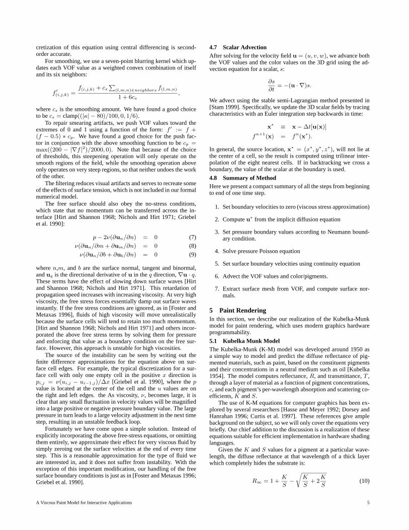
cretization of this equation using central differencing is second-order accurate.

For smoothing, we use a seven-point blurring kernel which up-dates each VOF value as a weighted convex combination of itselfand its six neighbors:

f ′(i,j,k) =f(i,j,k) + cs

∑(l,m,n)∈neighbors f(l,m,n)

1 + 6cs,

wherecs is the smoothing amount. We have found a good choiceto becs = clamp((|κ| − 80)/100, 0, 1/6).

To repair smearing artifacts, we push VOF values toward theextremes of 0 and 1 using a function of the form:f ′ := f +(f − 0.5) ∗ cp. We have found a good choice for the push fac-tor in conjunction with the above smoothing function to becp =max((200 − |∇f |2)/2000, 0). Note that because of the choiceof thresholds, this steepening operation will only operate on thesmooth regions of the field, while the smoothing operation aboveonly operates on very steep regions, so that neither undoes the workof the other.

The filtering reduces visual artifacts and serves to recreate someof the effects of surface tension, which is not included in our formalnumerical model.

The free surface should also obey the no-stress conditions,which state that no momentum can be transferred across the in-terface [Hirt and Shannon 1968; Nichols and Hirt 1971; Griebelet al. 1990]:

p− 2ν(∂un/∂n) = 0 (7)

ν(∂un/∂m+ ∂um/∂n) = 0 (8)

ν(∂un/∂b+ ∂ub/∂n) = 0 (9)

wheren,m, andb are the surface normal, tangent and binormal,anduq is the directional derivative ofu in theq direction,∇u · q.These terms have the effect of slowing down surface waves [Hirtand Shannon 1968; Nichols and Hirt 1971]. This retardation ofpropagation speed increases with increasing viscosity. At very highviscosity, the free stress forces essentially damp out surface wavesinstantly. If the free stress conditions are ignored, as in [Foster andMetaxas 1996], fluids of high viscosity will move unrealisticallybecause the surface cells will tend to retain too much momentum.[Hirt and Shannon 1968; Nichols and Hirt 1971] and others incor-porated the above free stress terms by solving them for pressureand enforcing that value as a boundary condition on the free sur-face. However, this approach is unstable for high viscosities.

The source of the instability can be seen by writing out thefinite difference approximations for the equation above on sur-face cell edges. For example, the typical discretization for a sur-face cell with only one empty cell in the positivex direction ispi,j = ν(ui,j − ui−1,j)/∆x [Griebel et al. 1990], where thepvalue is located at the center of the cell and theu values are onthe right and left edges. the As viscosity,ν, becomes large, it isclear that any small fluctuation in velocity values will be magnifiedinto a large positive or negative pressure boundary value. The largepressure in turn leads to a large velocity adjustment in the next timestep, resulting in an unstable feedback loop.

Fortunately we have come upon a simple solution. Instead ofexplicitly incorporating the above free-stress equations, or omittingthem entirely, we approximate their effect for very viscous fluid bysimply zeroing out the surface velocities at the end of every timestep. This is a reasonable approximation for the type of fluid weare interested in, and it does not suffer from instability. With theexception of this important modification, our handling of the freesurface boundary conditions is just as in [Foster and Metaxas 1996;Griebel et al. 1990].

4.7 Scalar AdvectionAfter solving for the velocity fieldu = (u, v, w), we advance boththe VOF values and the color values on the 3D grid using the ad-vection equation for a scalar,s:

∂s

∂t= −(u · ∇)s.

We advect using the stable semi-Lagrangian method presented in[Stam 1999]. Specifically, we update the 3D scalar fields by tracingcharacteristics with an Euler integration step backwards in time:

x∗ ≡ x−∆t[u(x)]

fn+1(x) = fn(x∗).

In general, the source location,x∗ = (x∗, y∗, z∗), will not lie atthe center of a cell, so the result is computed using trilinear inter-polation of the eight nearest cells. If in backtracking we cross aboundary, the value of the scalar at the boundary is used.

4.8 Summary of MethodHere we present a compact summary of all the steps from beginningto end of one time step.

1. Set boundary velocities to zero (viscous stress approximation)

2. Computeu∗ from the implicit diffusion equation

3. Set pressure boundary values according to Neumann bound-ary condition.

4. Solve pressure Poisson equation

5. Set surface boundary velocities using continuity equation

6. Advect the VOF values and color/pigments.

7. Extract surface mesh from VOF, and compute surface nor-mals.

5 Paint RenderingIn this section, we describe our realization of the Kubelka-Munkmodel for paint rendering, which uses modern graphics hardwareprogrammability.

5.1 Kubelka Munk ModelThe Kubelka-Munk (K-M) model was developed around 1950 asa simple way to model and predict the diffuse reflectance of pig-mented materials, such as paint, based on the constituent pigmentsand their concentrations in a neutral medium such as oil [Kubelka1954]. The model computes reflectance,R, and transmittance,T ,through a layer of material as a function of pigment concentrations,c, and each pigment’s per-wavelength absorption and scattering co-efficients,K andS.

The use of K-M equations for computer graphics has been ex-plored by several researchers [Hasse and Meyer 1992; Dorsey andHanrahan 1996; Curtis et al. 1997]. These references give amplebackground on the subject, so we will only cover the equations verybriefly. Our chief addition to the discussion is a realization of theseequations suitable for efficient implementation in hardware shadinglanguages.

Given theK andS values for a pigment at a particular wave-length, the diffuse reflectance at that wavelength of a thick layerwhich completely hides the substrate is:

R∞ = 1 +K

S−√K

S+ 2

K

S(10)

A Viscous Paint Model for Interactive Applications 5

For a finite layer of optical thickness,d, the reflectance and trans-mittance are given by

R =1

a+ b coth bSd(11)

T =b

a sinh bSd+ b cosh bSd, (12)

wherea = 1 + K/S andb =√a2 − 1. In the limit asd → ∞

Eqn. 11 reduces to Eqn. 10, andT → 0.If we have multiple pigments mixed together, each with their

ownK andS values and concentration by dry weightci, we cancompute theK andS of the mixture as

Kmix =∑i

ciKi

Smix =∑i

ciSi.

Finally, for two layersL1 andL2, withL2 on top ofL1, we cancompute the reflectance and transmittance of the optical composi-tion of the layers given their individualR andT values:

R12 = R2 +T 2

2R1

1−R1R2(13)

T12 =T1T2

1−R1bR2b

(14)

Note that in generalR12 6= R21, i.e. the reflectance of thetop of a composite is different from the reflectance of the bottom.Note also the reflectances in the denominator forT12 are bottomreflectances. The implication is that when computing the compo-sition of several layers, it is most efficient to compute the over-all combination from the bottom up, starting with the canvas re-flectanceR0. In this way, one avoids not only the cost of evaluatingEqn. 14 sinceT01...N is always zero, but also avoids having to com-pute the reverse reflectances of composites that would be requiredby Eqn. 14.

5.2 Hardware ImplementationFor efficient hardware implementation, first we have started by lim-iting the number of pigments to either four or eight in our prototype,so that the pigment concentrations can be stored in one or two stan-dard four-component RGBA textures. From these four or eight pig-ments, any arbitrary mixture can be made. If the initial primary pig-ments are widely separated in the colorspace, a large gamut of col-ors can be generated. In fact, the number of pigments and pigmenttextures is not the computational bottleneck in the hardware shader,so it is quite possible to expand the number of primary pigmentssomewhat beyond eight, with negligible performance penalty. Thebottleneck lies more in the software which must perform advectionon every pigment channel.

We useK and S values computed at the RGB color wave-lengths typically used in graphics, just as in [Curtis et al. 1997],and have used a similar method to the one presented there to deriveappropriate values forK andS.

We have implemented two different approaches to shading withK-M on hardware, a “thicker” style and a “thinner” style. The for-mer makes the assumption that the transmittance of the paint is verylow and thus the pigments at the surface completely hide the under-layers, allowing us to use theR∞ reflectance. For this we needto compute an interpolated value for pigment concentrations at thesurface location. We do this on a column-by-column basis as weperform the isosurface extraction.

The second rendering method composites the color of eachlayer of cells in the voxel grid using Eqn. 13. This requires a sepa-rate pass of the shader for each layer. After theN th pass, the frame

buffer holds the composited reflectance of the bottomN layers,and this reflectance is copied to a texture to use as the input basereflectance for passN + 1.

After computing the RGB diffuse reflectance of the pigmentmixture at each texel with the K-M equations, we complete theshading with a standard ambient-diffuse-specular light model. Weuse the surface normals computed in software from the VOF valuesto render the surface with bump mapping. The canvas and paintreflectance texture is also texture-mapped onto a quad to fill thescreen.

In our prototype we have used a voxel grid with 16 layers. Torender the composite of all these layers is quite expensive, evenwith a hardware shading language. To improve the performance wetypically window the computation to only perform the K-M shadingpass on portions of the canvas which have been modified. Oncecomputed, we can cache and reuse the total reflectance values formost of the canvas each frame.

5.3 Paint TransferFor depositing paint on the canvas using the brush, we have im-plemented some simple heuristics similar to those used in [Baxteret al. 2001]. We use the same surface mesh-based brush model aswell, but at the beginning of each time step the brush mesh is raster-ized onto the voxel grid and brush voxels tagged as wall boundarieswhich have their velocities set to the brush velocity, as discussed inSec. 3.4.

For simplicity, in the current system the brush is assumed tohave only a single color, but that color is continually blended withthe color of the paint it touches to allow the brush to “pick up”paint from the canvas. The amount of color change depends on thenumber and the color of voxels of paint in contact with the brush.

The brush color is used to update the color of any voxels itcomes in contact with, and the VOF values of cells adjacent to thebrush are pushed towards 1, so as to have the effect of depositingpaint volume on the surface. Additionally, during advection of theVOF and color fields, a color being advected from a cell with near-zero VOF is taken to have the brush color.

6 Results

Figure 5: Thick painting strokes created with our viscous paintmodel.

We have implemented our viscous paint model on a 2.5GHzPentium IV machine. Please see the accompanying video fordemonstrations of interaction with the paint model. When usedfor two-dimensional flow, our viscous free surface simulation runs

A Viscous Paint Model for Interactive Applications 6

Figure 6:An image hand-painted using our paint model.

at 64 × 64 resolution at over 70 frames per second with renderingof tracer particles. In three dimensions we can compute the flowon a32× 32× 16 grid at 20 frames per second. Since the methodis stable, the time step does not need to be reduced even when thefluid undergoes rapid motion. In contrast, a simulation restricted bythe CFL or viscosity timestep conditions would not be able to keepthe simulation synchronized with wall clock time, since it wouldhave to take many smaller substeps when fluid velocity is large.

We have integrated our paint model with a prototype paintingsystem to simulate an oil-paint-like medium. We provide the userwith a large canvas, then window the fluid simulation to calculateflow only in the immediate vicinity of the brush. This optimizationis reasonable since a very viscous paint medium essentially onlymoves in regions in which it is agitated. We render the results byextracting a height field and normal map from the paint fluid as de-scribed in Section 4.6. For the rendering we have implemented theKubelka-Munk reflectance model [Kubelka 1954] using fragmentprograms on an NVIDIA GeForceFX graphics board. This givesthe paint medium more realistic color mixing than is obtained fromsimple additive RGB blending [Hasse and Meyer 1992; Curtis et al.1997].

Fig. 5 shows an example of the type of effect produced by ourfluid model. Several images created by the users of our prototypepainting system are shown in Figs. 6-9. The abstract expressionistpainter in particular was fond of the paint model we have intro-duced. Notice the impasto style of the painting in Fig. 9. The ef-fects were created directly by the painter without any special imageprocessing. He also commented on the ease with which he was ableobtain a sense of depth in the paint and how this differered from thecommercial applications he has used. Most of the paintings werecreated by amateur artists within a couple of hours, without muchtraining or elaborate instruction. The footage in the supplemen-tary video demonstrates the interactive performance of our solverand the stable behavior of the viscous fluid generated by our paintmodel.

7 Summary and ConclusionIn this paper, we presented a novel viscous paint model for inter-active applications. The main characteristics of our viscous paintmodel include:

• An interactive viscous fluid model that captures the dynamicbehavior of impasto-like thick paint;

• Real-time color pigment mixing and compositing based onthe diffuse reflectance model described by Kubelka andMunk;

Figure 7:An image hand-painted using our paint model.

• Seamless integration with an interactive painting system us-ing an improved user interface and new, volumetric paint rep-resentation.

In the future we are interested in investigating fast methodsfor accurately enforcing conservation of volume, which the currentmodel does not do. Further work is also necessary to more accu-rately model the fluid-surface interface, especially in the case of aporous surface like canvas. Finally, the current model’s relativelycoarse resolution makes it unsuitable for very thin layers of mate-rial. We believe there is potential to combine our model with 2Dmethods to more accurately simulate of a wider variety of media.

ReferencesBAXTER, W., SCHEIB, V., L IN , M., AND MANOCHA, D. 2001. Dab: Haptic painting

with 3d virtual brushes.Proc. of ACM SIGGRAPH, 461–468.

CARLSON, M., MUCHA, P. J., R. BROOKS VAN HORN, I., AND TURK, G. 2002.Melting and flowing. InProceedings of the ACM SIGGRAPH symposium on Com-puter animation, ACM Press, 167–174.

CHEN, J., AND LOBO, N. 1995. Toward interactive-rate simulation of fluids withmoving obstacles using navier-stokes equations.Graphical Models and ImageProcessing(March), 107–116.

COCKSHOTT, T., PATTERSON, J., AND ENGLAND , D. 1992. Modelling the textureof paint. Computer Graphics Forum (Eurographics’92 Proc.) 11, 3, C217–C226.

CURTIS, C. J., ANDERSON, S. E., SEIMS, J. E., FLEISCHER, K. W., AND

SALESIN, D. H. 1997. Computer-generated watercolor. InProceedings of the24th annual conference on Computer graphics and interactive techniques, ACMPress/Addison-Wesley Publishing Co., 421–430.

DORSEY, J.,AND HANRAHAN , P. 1996. Modeling and rendering of metallic patinas.In SIGGRAPH 96 Conference Proceedings, Addison Wesley, H. Rushmeier, Ed.,Annual Conference Series, ACM SIGGRAPH, 387–396. held in New Orleans,Louisiana, 04-09 August 1996.

ENRIGHT, D., MARSCHNER, S., AND FEDKIW, R. 2002. Animation and render-ing of complex water surfaces. InProceedings of the 29th annual conference onComputer graphics and interactive techniques, ACM Press, 736–744.

FEDKIW, R., STAM , J., AND JENSEN, H. W. 2001. Visual simulation of smoke.In SIGGRAPH 2001, Computer Graphics Proceedings, ACM Press / ACM SIG-GRAPH, E. Fiume, Ed., 15–22.

FOSTER, N., AND FEDKIW, R. 2001. Practical animations of liquids. InSIGGRAPH2001, Computer Graphics Proceedings, ACM Press / ACM SIGGRAPH, E. Fiume,Ed., 23–30.

FOSTER, N., AND METAXAS, D. 1996. Realistic animation of liquids.Graphicalmodels and image processing: GMIP 58, 5, 471–483.

GOLUB, G. H., AND VAN LOAN, C. F. 1983. Matrix Computations. The JohnsHopkins University Press.

A Viscous Paint Model for Interactive Applications 7

Figure 8:An image hand-painted using our paint model.

GRIEBEL, M., DORNSEIFER, T., AND NEUNHOEFFER, T. 1990.Numerical Simula-tion in Fluid Dynamics: A Practical Introduction. SIAM Monographcs on Mathe-matical Modeling and Computation. SIAM.

HARLOW, F. H., AND WELCH, J. E. 1965. Numerical calculation of time-dependentviscous incompressible flow of fluid with free surface.The Physics of Fluids 8, 12(December), 2182–2189.

HASSE, C. S.,AND MEYER, G. W. 1992. Modeling pigmented materials for realisticimage synthesis.ACM Trans. on Graphics 11, 4, p.305.

HIRT, C. W., AND NICHOLS, B. D. 1981. Volume of fluid (vof) method for thedynamics of free boundaries.Journal of Computational Physics 39, 1, 201–225.

HIRT, C. W., AND SHANNON, J. P. 1968. Surface stress conditions forincompressible-flow calculations.Journal of Computational Physics 2, 403–411.

KASS, M., AND M ILLER , G. 1990. Rapid, stable fluid dynamics for computer graph-ics. In Proceedings of the ACM SIGGRAPH symposium on Computer animation,ACM Press, 49–57.

KUBELKA , P.,AND MUNK , F. 1931. Ein beitrag zur optik der farbanstriche.Z. techPhysik 12, 593.

KUBELKA , P. 1948. New contributions to the optics of intensely light-scatteringmaterial, part i.J. Optical Society 38, 448.

KUBELKA , P. 1954. New contributions to the optics of intensely light-scatteringmaterial, part ii: Non-homogenous layers.J. Optical Society 44, p.330.

NICHOLS, B. D., AND HIRT, C. W. 1971. Improved free surface boundary conditionsfor numerical incompressible-flow calculations.Journal of Computational Physics8, 434–448.

O’BRIEN, J. F.,AND HODGINS, J. K. 1995. Dynamic simulation of splashing fluids.In Computer Animation ’95, 198–205.

OSHER, S., AND FEDKIW, R. 2002. Level Set Methods and Dynamic Implicit Sur-faces. Applied Mathematical Sciences. Springer-Verlag.

SHEWCHUK, J. 1994. An introduction to the conjugate gradient method without theagonizing pain. Tech. Rep. CMUCS-TR-94-125, Carnegie Mellon University. (Seealso http://www.cs.cmu.edu/ quake-papers/painless-conjugate-gradient.ps.).

SMITH , A. R. 1978. Paint. TM 7, NYIT Computer Graphics Lab, July.

STAM , J. 1999. Stable fluids. InSiggraph 1999, Computer Graphics Proceedings,Addison Wesley Longman, Los Angeles, A. Rockwood, Ed., 121–128.

X. WEI, W. L., AND KAUFMAN , A. 2003. Interactive melting and flowing of viscousvolumes.Proc. of Computer Animation and Social Agents.

Figure 9: A painting by abstract expressionist painter, John Hol-loway

A Viscous Paint Model for Interactive Applications 8