Aalborg Universitet Generation and Assessment of Urban ...vbn.aau.dk/...H_hle_Generation_and_Assessment_of_Urban_Land_Cov… · Generation and Assessment of Urban Land Cover Maps

Aalborg Universitet

Generation and Assessment of Urban Land Cover Maps Using High-ResolutionMultispectral Aerial ImagesHøhle, Joachim; Höhle, Michael

Published in:International Journal on Advances in Software

Publication date:2013

Document VersionEarly version, also known as pre-print

Link to publication from Aalborg University

Citation for published version (APA):Höhle, J., & Höhle, M. (2013). Generation and Assessment of Urban Land Cover Maps Using High-ResolutionMultispectral Aerial Images. International Journal on Advances in Software, 6(3 & 4), 272-282.

General rightsCopyright and moral rights for the publications made accessible in the public portal are retained by the authors and/or other copyright ownersand it is a condition of accessing publications that users recognise and abide by the legal requirements associated with these rights.

? Users may download and print one copy of any publication from the public portal for the purpose of private study or research. ? You may not further distribute the material or use it for any profit-making activity or commercial gain ? You may freely distribute the URL identifying the publication in the public portal ?

Take down policyIf you believe that this document breaches copyright please contact us at [email protected] providing details, and we will remove access tothe work immediately and investigate your claim.

Downloaded from vbn.aau.dk on: september 01, 2018

http://vbn.aau.dk/en/publications/generation-and-assessment-of-urban-land-cover-maps-using-highresolution-multispectral-aerial-images(9de4abfa-c0fa-4ae8-bdfd-933ca75497d8).html

272

International Journal on Advances in Software, vol 6 no 3 & 4, year 2013, http://www.iariajournals.org/software/

2013, © Copyright by authors, Published under agreement with IARIA - www.iaria.org

Generation and Assessment of Urban Land Cover Maps Using High-Resolution Multispectral Aerial Cameras

Joachim Höhle Department of Planning, Aalborg University

Aalborg, Denmark Email: [email protected]

Michael Höhle Department of Mathematics, Stockholm University

Stockholm, Sweden Email: [email protected]

Abstract—New aerial cameras and new advanced geo-processing tools improve the generation of urban land cover maps. Elevations can be derived from stereo pairs with high density, positional accuracy, and efficiency. The combination of multispectral high-resolution imagery and high-density elevations enable a unique method for the automatic generation of urban land cover maps. In the present paper, imagery of a new medium-format aerial camera and advanced geoprocessing software are applied to derive normalized digital surface models and vegetation maps. These two intermediate products then become input to a tree structured classifier, which automatically derives land cover maps in 2D or 3D. We investigate the thematic accuracy of the produced land cover map by a class-wise stratified design and provide a method for deriving necessary sample sizes. Corresponding survey adjusted accuracy measures and their associated confidence intervals are used to adequately reflect uncertainty in the assessment based on the chosen sample size. Proof of concept for the method is given for an urban area in Switzerland. Here, the produced land cover map with six classes (building, wall and carport, road and parking lot, hedge and bush, grass) has an overall accuracy of 86% (95% confidence interval: 83-88%) and a kappa coefficient of 0.82 (95% confidence interval: 0.78-0.85). The classification of buildings is correct with 99% and of road and parking lot with 95%. To possibly improve the classification further, classification tree learning based on recursive partitioning is investigated. We conclude that the open source software “R” provides all the tools needed for performing statistical prudent classification and accuracy evaluations of urban land cover maps.

Keywords-land cover map; classification; assessment; thematic accuracy; multispectral camera; map revision

I. INTRODUCTION Land cover maps are an important product of the

mapping and GIS industry. The coverage of the landscape with vegetation, soil or man-made constructions may be automatically mapped and analysed. Images taken from an airplane or a satellite are used to derive land cover maps automatically. The intensity values of picture elements (pixels) in different bands of multispectral images are used to determine the different types of objects. It is difficult to distinguish between objects on the ground and objects above the ground, e.g., between buildings and parking lots or trees and hedges. Land cover maps can be generated with a higher thematic accuracy when information on elevations is

included [1]. Today, advanced processing tools are able to generate elevations of high accuracy and density from imagery [2]. The generation of land cover maps and their applications will benefit from these innovations.

Of special interest are built-up areas where small objects have to be mapped and where changes over time frequently occur. For such areas, land cover maps have to be produced by means of high-resolution images. Their ground sampling distance (GSD) is a few centimeters. The use of a new high-resolution multispectral aerial camera will be a characteristic of this contribution. In addition, the applied methodology uses a new approach in mapping. The images are used for the generation of a point cloud of high density and of regular structure (grid). Besides the spatial coordinates of a geodetic reference system and a map projection (e.g., easting, northing, and elevation) the individual points may also have attributes such as “height above ground” and “vegetation index”. The land cover map is generated by a classification procedure and the result is then visualized by simple plot commands. In order to assess the thematic accuracy of the land cover maps, one typically selects a sample of points in the map, derives their true classes using manual procedures and then extrapolates the accuracy results to the entire map using statistical principles [3].

The outline of this paper is as follows: After the introduction (Section I) the state of the art in the generation of land cover maps is discussed and our aims are formulated (Section II). The new generation of aerial cameras and processing tools is presented in Sections III and IV. Our method for the generation of urban land cover maps is explained in Section V. Special attention is given to the accuracy assessment of these land cover maps (Section VI). In Section VII our method is applied to a test area in Switzerland. The obtained results on the test area are evaluated in Sections VIII and IX. A conclusion on the work carried out and suggestions for future work end the paper (Section X).

II. LAND COVER MAPS AND THEIR APPLICATIONS Land cover maps have a number of different classes

(categories), which are visualized in a two-dimensional (2D) map by different colours. The standard methods classify the images by means of training areas where the truth (reference) is known from field work or manual interpretation of images. The automatic classification of the images uses the intensity values of image elements (pixels) in different bands of the

273



images and applies various statistical methods. More advanced methods form larger areas (objects) first and classify them in a second step. This object-based classification uses a number of attributes like shape, size, and texture and generates land cover. The land cover map has to be georeferenced. This means that the orientation of the images and a digital terrain model (DTM) have to be known in advance. The classification may use the original images or orthoimages - in the first case the classification result has to be rectified and orthogonalized. The derived land cover map is assessed by a few independent check points or check areas. The results are presented by means of an error (confusion) matrix.

The usage of elevations as an attribute of objects has been tried before. In [1], a solution for automatic generation of land cover maps has been proposed and applied to a one hectare large test area. Elevations, heights, and vegetation indices have been derived from images only. True-colour orthoimages and false-colour stereo pairs were used for the determination of the reference. The overall accuracy of the derived land cover map with four classes (building, road and parking lot, tree and hedge) has been 79%. The use of stereo-vision was the preferred approach in the assessment of the thematic accuracy.

In [4], elevations were derived from laser scanning and have been used together with aerial images and cadastre maps for the generation of a land cover map. Ten urban and seven agriculture classes have been determined for the city of Valencia/Spain. The overall accuracy of the derived land cover map was 85%. Reference [5] describes an object-oriented classification where 81% of all residential buildings are correctly determined for a test area located in Austin, Texas/U.S.A. Attributes of objects are derived from laser scanning, aerial images, and road maps.

Machine learning algorithms are applied for the urban land cover classification in [6]. The classification can either be based on pixels or object features. A combination of pixels, object features (area, length, etc.), and layer values (mean, standard deviation, etc.) has been suggested in Reference [7].

A land cover map has many applications and can be used for all types of planning. View shed analysis and studies of propagation of noise or electromagnetic waves are applications in engineering. An important application is the revision of topographic data bases. This task requires a high positional and thematic accuracy. In order to detect changes and errors in topographic databases the generation of a land cover map may be the first step in the revision process. The superimposition of the land cover map with the topographic database will indicate which objects of the topographic database have to be added, deleted, or changed in size or shape. Recent studies in revision of topographic databases are carried out in [8] [9]. The exact actions depend on what types of data have to be revised. There are topographic databases in 2D, 2.5D, and 3D. Sometimes, the important objects are updated only, e.g., buildings, roads, and trees. Land cover maps are also used for studies in town development. The changes in areas of buildings, traffic, and vegetation over several years are studied in [10]. In that

investigation, the land cover maps are derived from vector maps and low-resolution satellite images. The applied classification of the images uses intensity values of pixels only.

Thus, our aims for this paper are: 1) Generation of urban land cover maps by applying decision trees based on height and vegetation information derived from a new type of aerial images. 2) Assessing the thematic accuracy using overall and class specific accuracy measures. 3) To do so by a class-wise stratified sampling design of reference points, which allows for precise estimation of per class accuracy quantities. 4) To illustrate that all the necessary computation can be done by “R” and its extension packages.

In comparison to the investigation in [1] we now focus here on the accuracy assessment as point estimates and confidence intervals in the light of a class-stratified sampling design. Furthermore, classification is now improved using additional classes, and a comparison is made with machine learning derived decision trees. Finally, all computations in the proof-of-example section are now based on a larger test area than previously.

III. NEW DIGITAL AERIAL CAMERAS With the development of new advanced digital aerial

cameras, the generation of land cover maps has new tools at its disposal. There are different types and models of aerial cameras. Three of the most advanced cameras will be discussed in the following: the Hexagon/Intergraph DMCII 250, the Microsoft UltraCam Eagle, and the Hexagon/Leica Geosystems RCD30 camera. Details of the cameras are described in publications [11] [12] [13]. All three cameras are frame cameras, which can produce images of high resolution and high geometric quality. They are designed for mapping tasks. The produced images have different features; the major ones are listed in Table I.

There is a considerable difference in the format of the output image. The RCD30 is a medium-format camera; the other two cameras are considered as large-format cameras. A larger format requires less flying time in order to cover an area to be mapped assuming that the images of all cameras have the same GSD. The necessary length of the flight is an economic factor, and large-format cameras have an advantage in projects covering large areas. All three cameras can produce black & white, colour, and false-colour images simultaneously. Newly designed lenses match the resolution of the sensors and make high image quality possible. The

TABLE I. FEATURES OF THREE NEW DIGITAL AERIAL CAMERAS

Features UC Eagle

DMCII 250

RCD30

pixel size [µm] 5.2 5.6 6.0 focal length [mm] 80 112 50, 80 image size (in flight direction) [pel] [mm]

13 080 68.0

14 656 82.1

6708 40.2

image size (across flight direction) [pel] [mm]

20010 104.1

17216 96.4

8956 53.7

number of pixels per image [MP] 262 252 60

274



cameras are calibrated, and the obtained calibration data are used to correct the images in geometry and radiometry. Additional sensors for position (GNSS) and attitude can be supplemented and will support accurate georeferencing of the imagery. More details have to be mentioned on the RCD30 camera because its images will be used in the following examples. The colour images are produced from one charge-coupled device (CCD) with Bayer filters. The infra-red band is imaged by a second CCD of the same high resolution (pixel size=6 µm x 6 µm). Image motion is compensated mechanically in two axes. The output images are corrected for distortion, light-fall off of the lens, and non-uniformity for dark signals. Two different lenses can be used without the need of re-calibration. In order to obtain images with GSD=0.05 m, they have to be taken from 417 m above ground with a 50 mm lens. One frame will cover 0.15 km2 on the ground. A gyro-stabilized mount can be used which will prevent big tilts of the imagery.

IV. NEW PROCESSING TOOLS The generation of land cover maps from images requires

the use of specific software tools. They span from general image processing to dedicated software for photogrammetry, remote sensing, and geographic information systems (GIS). The characteristic of our approach is the use of digital elevation models, which are derived from high-resolution images. The latest developments in this field may enhance the performance of the previously suggested approach of the generation of land cover maps [1]. One of the problems to overcome is the large amount of data, which might make it necessary to divide the work into smaller units. One 64-bit computer with 8 GB RAM (as is at disposal in this investigation) is not an optimal processor for this task. More computer power is necessary to solve the task for large areas. The many different software tools are expensive if they have to be acquired from commercial software vendors. However, an increasing amount of freeware and open source tools has become available to conduct some of the tasks. Such tools are preferred whenever possible. Specifically, we use the open-source software environment “R” [14] for statistical computing and visualization and, hence, one aim of the present paper is to demonstrate its use in the generation and assessment of land cover maps.

A. Programs for the generation of digital elevation models Digital elevation models can automatically be derived

from two or more images covering the same area on the ground. Corresponding image parts are matched using the intensity values of image elements (pixels). Spatial ground coordinates are intersected by means of the corresponding pixels in two or more georeferenced images. The resulting point cloud can be transferred into a regular grid of points representing a digital surface model (DSM). Such software programs are pretty complex and their development requires many man years. Professional programs are, therefore, expensive. Many parameters have to be tuned by the user in order to derive elevations of high accuracy and

completeness, which in turn means that some expertise is necessary in order to derive good results.

The problems to be overcome are the huge amount of data and the mismatches due to the lack of contrast and structure in the images. International tests reveal elevation accuracies of RMSEZ=4cm at large-scale images with GSD=8 cm [15]. The density of the point cloud may be extremely high, e.g., 156 points/m2 at GSD=8 cm [16]. This means that the derived DSM may have the resolution of the images. The use of distributed processing and dedicated hardware make a high performance in the calculations possible. Reference [17] reports about a benchmark test where 997 million points are derived from 1562 images (filling 1.44 TB) in 2.5 hours or six seconds/image.

The DSM is an intermediate product only. For the generation of land cover maps the heights of the objects (buildings, trees, etc.) are required. This is accomplished by filtering the DSM so that only elevations of the bare earth (terrain) will remain. This process requires editing and checking. From the remaining terrain points a grid of elevations is interpolated, which represents a DTM. The editing software is a complex software tool, which allows for measuring, correcting, and visualizing of 3D data. The difference between DSM and DTM is the normalized DSM (nDSM), which is the required input of the classification program. The nDSM is derived using a C++ program, which performs the matching between the two point clouds by using a linear search to identify the first neighbour within a distance of 0.05 m. As a consequence, the search of corresponding elevations in the two elevation models (DSM and DTM) is quite time-consuming. Improvements could be obtained by exploiting the spatial structure of the data in the search.

B. Programs for the generation and assessment of urban land cover maps The generation of the land cover map and the assessment

of the results are developed using the statistical software environment “R”, which is an open source environment for statistical computing and graphics. The programming can be both object-oriented and functional in style. Furthermore, a large number of open source extension packages (created by an active community) provide the newest methodological functionality for many visualization and statistical tasks. For example, the package “survey” [18] can be used for computing accuracy measures in complex survey situations, “rpart” [19] implements recursive partitioning for classification trees, and “vrmlgen” enables the visualization of land cover maps in 3D [20].

V. APPLIED METHOD FOR THE GENERATION OF LAND COVER MAPS

The applied method uses the nDSM derived from images and supplements it with additional attributes. The points of the nDSM are arranged in a regular grid of high density. The spacing between points has been selected as a multiple of the image element (pixel) on the ground. The new unit is called a cell in the 2D space or cube in the 3D space. The attributes to be added characterize the object to be mapped. They are

275



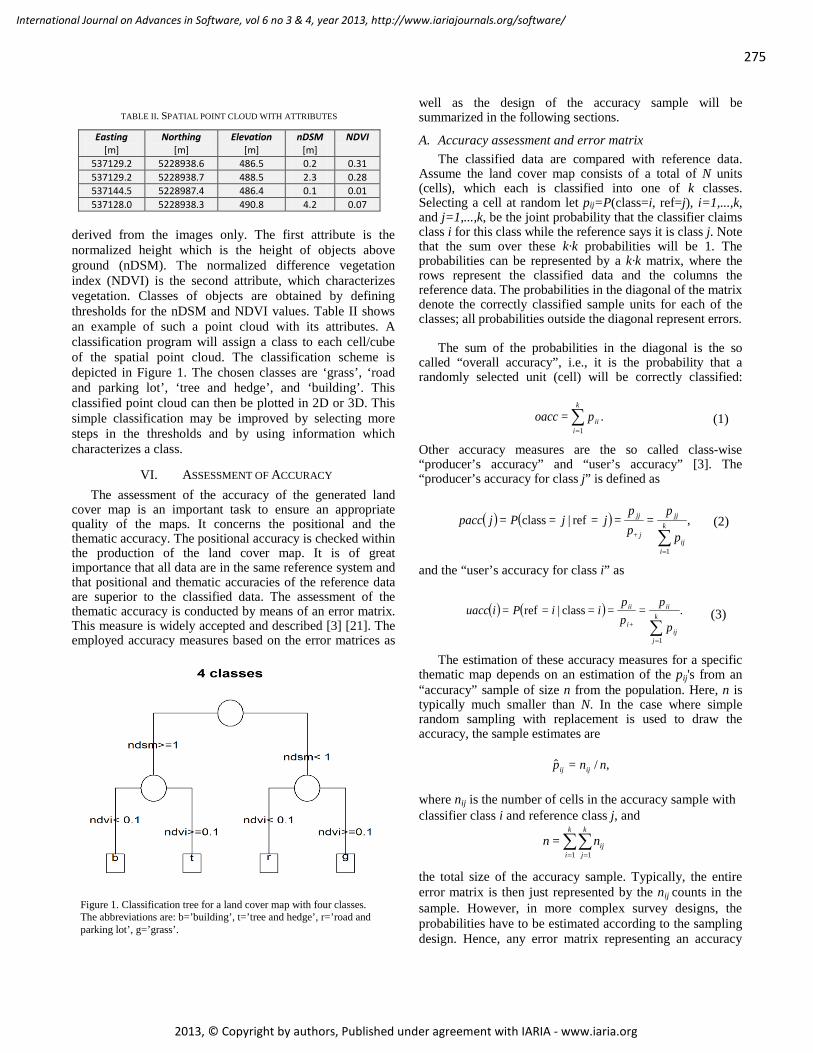
derived from the images only. The first attribute is the normalized height which is the height of objects above ground (nDSM). The normalized difference vegetation index (NDVI) is the second attribute, which characterizes vegetation. Classes of objects are obtained by defining thresholds for the nDSM and NDVI values. Table II shows an example of such a point cloud with its attributes. A classification program will assign a class to each cell/cube of the spatial point cloud. The classification scheme is depicted in Figure 1. The chosen classes are ‘grass’, ‘road and parking lot’, ‘tree and hedge’, and ‘building’. This classified point cloud can then be plotted in 2D or 3D. This simple classification may be improved by selecting more steps in the thresholds and by using information which characterizes a class.

VI. ASSESSMENT OF ACCURACY The assessment of the accuracy of the generated land

cover map is an important task to ensure an appropriate quality of the maps. It concerns the positional and the thematic accuracy. The positional accuracy is checked within the production of the land cover map. It is of great importance that all data are in the same reference system and that positional and thematic accuracies of the reference data are superior to the classified data. The assessment of the thematic accuracy is conducted by means of an error matrix. This measure is widely accepted and described [3] [21]. The employed accuracy measures based on the error matrices as

well as the design of the accuracy sample will be summarized in the following sections.

A. Accuracy assessment and error matrix The classified data are compared with reference data.

Assume the land cover map consists of a total of N units (cells), which each is classified into one of k classes. Selecting a cell at random let pij=P(class=i, ref=j), i=1,...,k, and j=1,...,k, be the joint probability that the classifier claims class i for this class while the reference says it is class j. Note that the sum over these k·k probabilities will be 1. The probabilities can be represented by a k·k matrix, where the rows represent the classified data and the columns the reference data. The probabilities in the diagonal of the matrix denote the correctly classified sample units for each of the classes; all probabilities outside the diagonal represent errors.

The sum of the probabilities in the diagonal is the so

called “overall accuracy”, i.e., it is the probability that a randomly selected unit (cell) will be correctly classified:

Other accuracy measures are the so called class-wise “producer’s accuracy” and “user’s accuracy” [3]. The “producer’s accuracy for class j” is defined as

and the “user’s accuracy for class i” as

The estimation of these accuracy measures for a specific

thematic map depends on an estimation of the pij's from an “accuracy” sample of size n from the population. Here, n is typically much smaller than N. In the case where simple random sampling with replacement is used to draw the accuracy, the sample estimates are

,/ˆ nn=p ijij

where nij is the number of cells in the accuracy sample with classifier class i and reference class j, and

the total size of the accuracy sample. Typically, the entire error matrix is then just represented by the nij

counts in the

sample. However, in more complex survey designs, the probabilities have to be estimated according to the sampling design. Hence, any error matrix representing an accuracy

∑∑= =

k

i

k

jijn=n

1 1

( ) ( ) .classref

1∑

=

k

jij

ii

+i

ii

p

p=

pp

=i=|i=P=iuacc (3)

( ) ( ) ,refclass

1∑

=

k

iij

jj

j+

jj

p

p=

pp

=j=|j=P=jpacc (2)

.1

∑=

k

iiip=oacc (1)

TABLE II. SPATIAL POINT CLOUD WITH ATTRIBUTES

Easting [m]

Northing [m]

Elevation [m]

nDSM [m]

NDVI

537129.2 5228938.6 486.5 0.2 0.31 537129.2 5228938.7 488.5 2.3 0.28 537144.5 5228987.4 486.4 0.1 0.01 537128.0 5228938.3 490.8 4.2 0.07

Figure 1. Classification tree for a land cover map with four classes. The abbreviations are: b=’building’, t=’tree and hedge’, r=’road and parking lot’, g=’grass’.

276



sample has to be accompanied by a statement of the selected sample design in order to facilitate proper estimation.

To assess the thematic accuracy of the land cover map by the above measures, one has to decide on an adequate design and sample size of the accuracy sample. Since one of our aims is to estimate user accuracy for each class up to a given precision we use a stratified simple random (STSI) sampling, selecting nc samples for each class by simple random sampling (without replacement) and, hence, a total sample size of n=k·nc. In the subsequent analyses of our stratified accuracy sample it is, thus, important to take the stratification into account, because classes might be over- or under-sampled compared to their overall distribution in the map. In this case (and ignoring any finite population correction), we will use

( ) ( )+iijiij nnNN=p //ˆ ⋅

as estimates [27], where Ni is the total number of units in the population, which are of class i and

∑ =

k

j ij+i n=n1

is the number of units in the accuracy sample, which have classifier class i. A particular strength of “R” is here the availability of the package "survey" [18], which facilitates the computation of such survey weighted accuracy measures - even in complex survey situations. As an example, the above stratified design is easily specified using the svydesign function after which the accuracy measures can be computed using the function svyciprop.

B. Reference data The reference data should be independent, of high

accuracy, and reliable. The collection of the reference data has to be carried out nearly at the same point of time as the production of the land cover map, so that a change in the landscape and vegetation will not have an effect on the results of the assessment. The efforts for collecting reference data have to be economically justified, i.e., they should be a fraction of the costs for generating the land cover map.

It may be difficult to fulfil all of these requirements. The land cover map is generated from a vegetation map (derived from false-colour orthoimages based on a DTM) and a normalized DSM. Both digital elevation models are automatically derived from images in true colour. The reference data may be derived by manual photointerpretation using false-colour stereo pairs and manual measurements of elevation differences. The orientation data of the images are determined by some ground control (measured by means of GNSS) and tie point measurements in the images. The orientation data of the images are the same both for the generation of the map and for the assessment.

C. Sample size determination and confidence intervals Since per class user accuracy can be thought of as the

probability p for a correct classification in a binomial experiment with x successes in n trials, one way to determine

sample size is by specification of the desired width of the resulting 95% confidence interval (CI) for this proportion p. We will use likelihood ratio test (LRT) based confidence intervals for this proportion, because such intervals have better coverage probabilities than the standard Wald intervals often used in remote sensing [22]. Here, coverage probability of a CI refers to the proportion of times the CI will cover the true value of p (when thinking of an infinite number of hypothetical repetitions). The better coverage of LRT CIs is especially pronounced if p is near zero or one, respectively, or if the sample size is small. As an example, a 95% Wald CI in the situation where n=21 and p=0.85 will have an actual coverage probability of just 84%, which is far away from the nominal 95%, whereas a 95% LRT interval has a coverage probability of 94%.

LRT intervals for the proportion p are constructed by inversion of the LRT test for the hypothesis H0: p=p0 vs. H1: p≠p0 [23]. That is, the lower and upper limit of a 95% LRT CI are found numerically as the boundary values of p0 solving the inequality

Here, Λn,x(p0) denotes the likelihood ratio between p0 and the maximum likelihood estimate nxp /ˆ = , i.e.,

( ) ( )( ) xnx

xnx

xn, pppp=pΛ −

−

−−

ˆ1ˆ1 00

0,

and χ2

0.95(1)≈3.841 denotes the 95% quantile of the χ2

distribution with one degree of freedom. Implementation of such LRT intervals can be found in the “R” package “binom” [24]. Assuming a worst-case user accuracy of about 60% for each class and a desired half-width of no more than w=10%, one can sequentially increase the sample size n until the confidence interval for p has a width smaller than 2·w when using the observation x=0.6·n. The “R” package “sampleSizeBinom” [25], which implements this procedure, obtains a required sample size of n=91 per class. Hence, our stratified accuracy sample when using 4 classes will totally consist of 91·4=364 units. In order to compute the previously described LRT confidence intervals also for the survey weighted accuracy measures, we use the procedure suggested by Rao and Scott [26], which is implemented as part of the function svyciprop in the "survey" package.

D. Kappa analysis A further measure of agreement between two raters, who

both classify a number of items into each of k categories, is Cohen's κ [21], which can be viewed as chance adjusted agreement measure defined as follows:

∑

∑∑

=

==

−

−

k

ii++i

k

ii++i

k

iii

pp

ppp=κ

1

11

1(5)

( )( ) .ln2 0.9502

xn, χpΛ ≤⋅− (4)

277



Landis and Koch [27] characterize κ-values between 0.41 and 0.60 as moderate, 0.61–0.80 as substantial, and 0.81–1 as almost perfect agreement between the classification and the reference data. An estimate for κ is found by replacing pii, pi+, and p+i in (5) with the respective survey adjusted estimates. If one, however, ignores the sampling design underlying the numbers in the error matrix, and just uses the raw survey-unadjusted estimates for the p’s, the obtained κ estimate will be biased. For example, if a particular poorly classified class is over-sampled, the obtained κ estimate might be too low.

For a STSI design, formulae for computing κ from the resulting error matrix can be found in [28]. In [28], the formulae are an instance of a more general technique for calculating point estimates and variances for transformations of survey weighted estimates (see, e.g., [29]).

To reflect uncertainty in the estimation of κ it is also prudent to specify a corresponding (1-α)·100% CI. Again, [30] presents equations for computing the variance of the estimate, which enables the computing of Wald CIs for the stratified case. Note that the package “survey” contains the function svykappa to directly compute the survey weighted κ estimate and associated Wald CIs based on the general equations in [29] – this even works for more complex survey designs. It has to be remarked that the use of κ to assess classifier performance in remote sensing is somewhat debated [30], because κ is directly linked to the overall accuracy, but its scale is harder to interpret. Still, we report κ estimates here as a supplement measure to the overall accuracy, since κ just as the overall and user's accuracy is particularly easy to calculate with “R” – even in the case of a complex design of the accuracy sample. In summary, the principle in the assessment of the thematic accuracy is depicted in Figure 2.

As accuracy measures the survey weighted overall accuracy and Cohens’s κ, as well as the producer’s and user’s accuracy for each class are selected. Each measure is supported by a corresponding CI in order to quantify the uncertainty in its estimation. Altogether, one of our points is that a per-class stratified sampling approach for the assessment of thematic accuracy is easily handled with “R”. Such an approach provides reliable estimates for the

accuracy of each class.

VII. PRACTICAL EXAMPLE A practical investigation is conducted for a residential

area in Switzerland to evaluate the proposed approach. The area consisting of buildings, car ports, roads, parking lots as well as trees, hedges, and grassland is photographed from the air. The size of the test area is about 1.6 hectares.

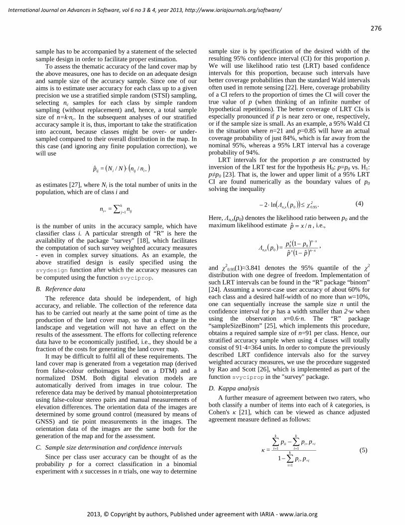
The first land cover map comprises the four classes ‘building’, ‘tree and hedge’, ‘grass’, ‘road and parking lot’ only. The steps in the generation of the land cover map are depicted in Figure 3. True colour images are used to derive a very dense 3D point cloud by means of matching corresponding image parts. The point cloud is then transformed into a gridded DSM using interpolation techniques. Through a process of filtering, which removes elevations above ground as well as blunders, a DTM is generated. Then, the difference between the DSM and the DTM, the nDSM, can be derived. The DTM is also used for the production of a false colour orthoimage, which is further processed to a NDVI map containing two classes (vegetation, non-vegetation). NDVI and nDSM information is used to produce a point cloud with two attributes (nDSM, NDVI). The land cover map is produced by classification of

Figure 3. Steps in the production of a land cover map [1]. Colour and false-colour aerial images are used to derive accurate and dense height data (nDSM), which are supplemented with vegetation data (NDVI). Such an ‘intelligent’ 3D point cloud is input to a classification scheme, which generates the land cover map.

Figure 2. Principle of the applied assessment of the thematic accuracy.

278



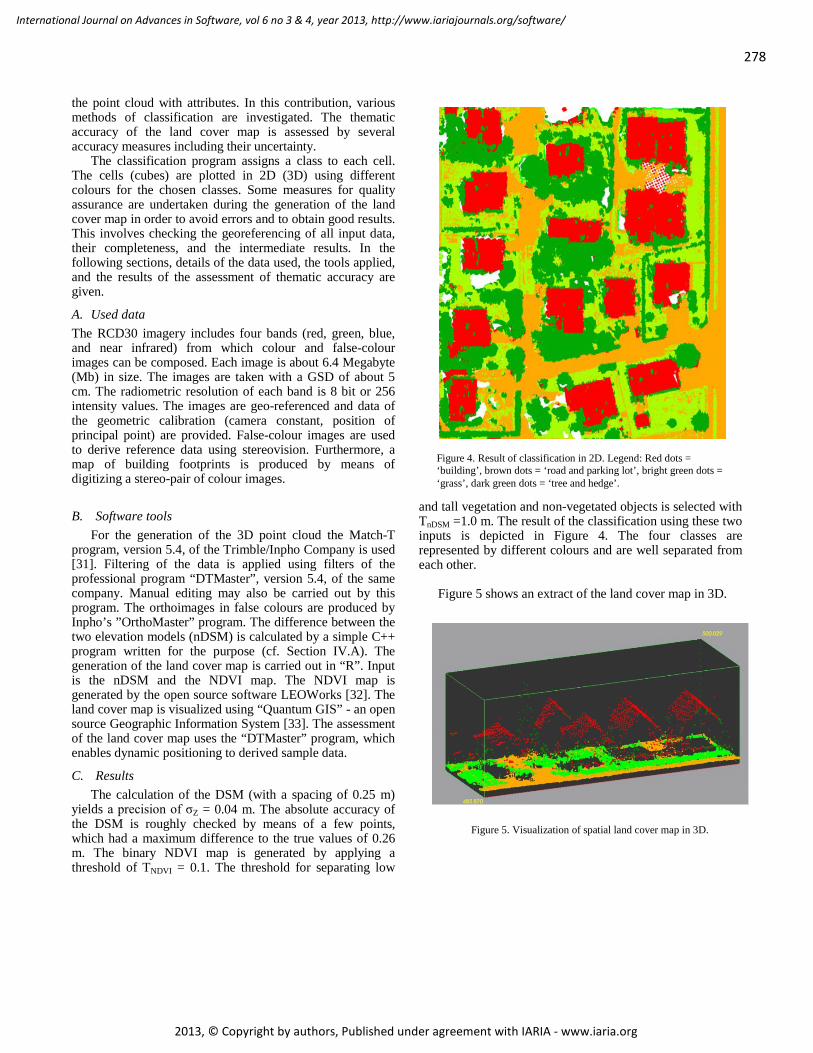
Figure 5. Visualization of spatial land cover map in 3D.

the point cloud with attributes. In this contribution, various methods of classification are investigated. The thematic accuracy of the land cover map is assessed by several accuracy measures including their uncertainty.

The classification program assigns a class to each cell. The cells (cubes) are plotted in 2D (3D) using different colours for the chosen classes. Some measures for quality assurance are undertaken during the generation of the land cover map in order to avoid errors and to obtain good results. This involves checking the georeferencing of all input data, their completeness, and the intermediate results. In the following sections, details of the data used, the tools applied, and the results of the assessment of thematic accuracy are given.

A. Used data The RCD30 imagery includes four bands (red, green, blue, and near infrared) from which colour and false-colour images can be composed. Each image is about 6.4 Megabyte (Mb) in size. The images are taken with a GSD of about 5 cm. The radiometric resolution of each band is 8 bit or 256 intensity values. The images are geo-referenced and data of the geometric calibration (camera constant, position of principal point) are provided. False-colour images are used to derive reference data using stereovision. Furthermore, a map of building footprints is produced by means of digitizing a stereo-pair of colour images.

B. Software tools For the generation of the 3D point cloud the Match-T

program, version 5.4, of the Trimble/Inpho Company is used [31]. Filtering of the data is applied using filters of the professional program “DTMaster”, version 5.4, of the same company. Manual editing may also be carried out by this program. The orthoimages in false colours are produced by Inpho’s ”OrthoMaster” program. The difference between the two elevation models (nDSM) is calculated by a simple C++ program written for the purpose (cf. Section IV.A). The generation of the land cover map is carried out in “R”. Input is the nDSM and the NDVI map. The NDVI map is generated by the open source software LEOWorks [32]. The land cover map is visualized using “Quantum GIS” - an open source Geographic Information System [33]. The assessment of the land cover map uses the “DTMaster” program, which enables dynamic positioning to derived sample data.

C. Results The calculation of the DSM (with a spacing of 0.25 m)

yields a precision of σZ = 0.04 m. The absolute accuracy of the DSM is roughly checked by means of a few points, which had a maximum difference to the true values of 0.26 m. The binary NDVI map is generated by applying a threshold of TNDVI = 0.1. The threshold for separating low

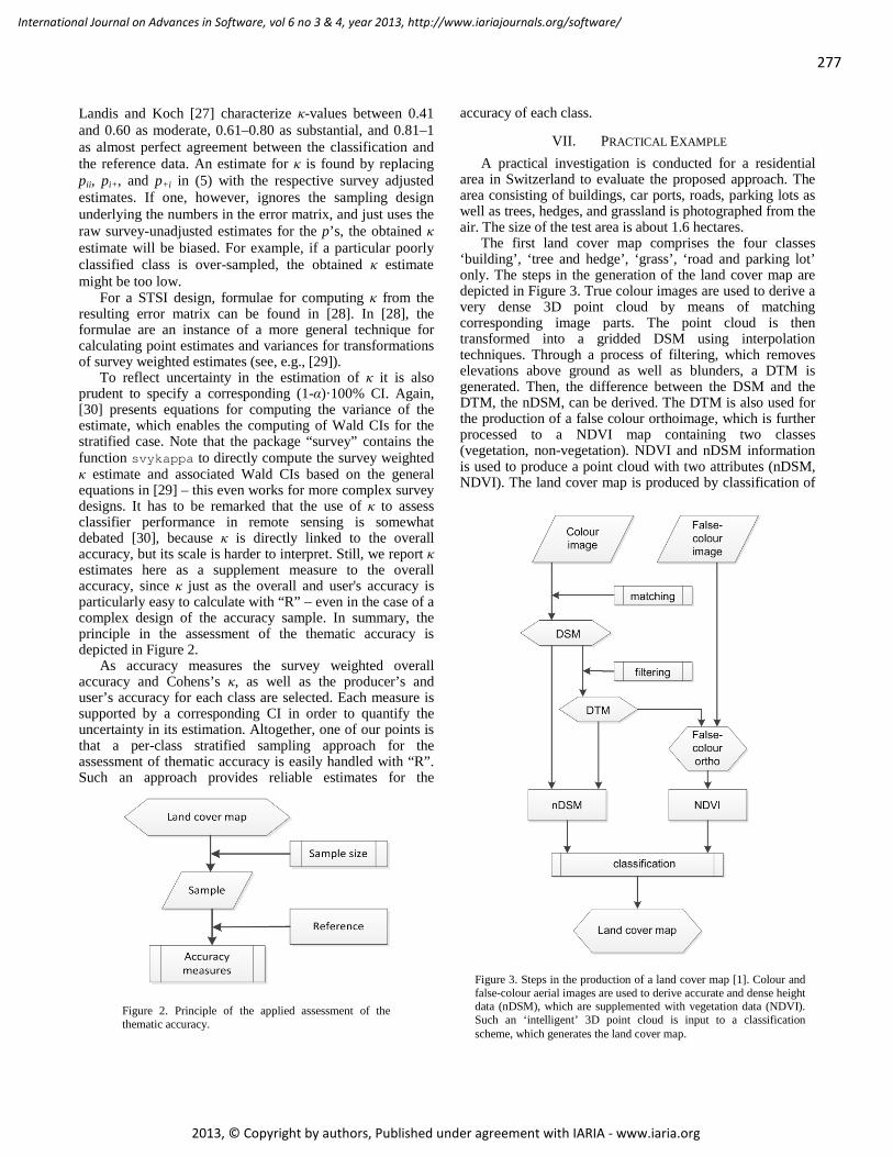
and tall vegetation and non-vegetated objects is selected with TnDSM =1.0 m. The result of the classification using these two inputs is depicted in Figure 4. The four classes are represented by different colours and are well separated from each other.

Figure 5 shows an extract of the land cover map in 3D.

Figure 4. Result of classification in 2D. Legend: Red dots = ‘building’, brown dots = ‘road and parking lot’, bright green dots = ‘grass’, dark green dots = ‘tree and hedge’.

279



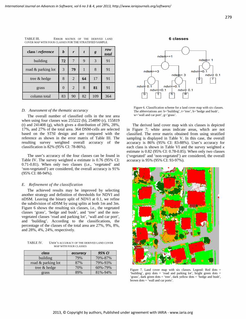
D. Assessment of the thematic accuracy The overall number of classified cells in the test area

when using four classes was 255222 (b), 254890 (r), 155819 (t) and 241408 (g), which gives a distribution of 28%, 28%, 17%, and 27% of the total area. 364 DSM-cells are selected based on the STSI design and are compared with the reference as shown in the error matrix of Table III. The resulting survey weighted overall accuracy of the classification is 82% (95% CI: 78-86%).

The user’s accuracy of the four classes can be found in

Table IV. The survey weighted κ estimate is 0.76 (95% CI: 0.71-0.81). When only two classes (i.e., ‘vegetated’ and ‘non-vegetated’) are considered, the overall accuracy is 91% (95% CI: 88-94%).

E. Refinement of the classification The achieved results may be improved by selecting

another strategy and definition of thresholds for NDVI and nDSM. Leaving the binary split of NDVI at 0.1, we refine the subdivision of nDSM by using splits at both 1m and 3m. Figure 6 shows the resulting six classes, i.e., the vegetated classes ‘grass’, ‘hedge and bush’, and ‘tree’ and the non-vegetated classes ‘road and parking lot’, ‘wall and car port’, and ‘building’. According to the classifications, the percentage of the classes of the total area are 27%, 9%, 8%, and 28%, 4%, 24%, respectively.

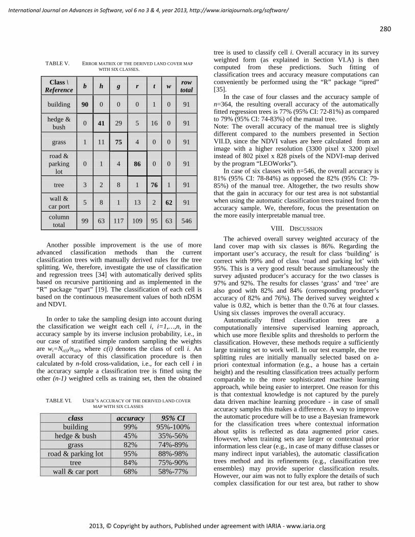
The derived land cover map with six classes is depicted

in Figure 7; white areas indicate areas, which are not classified. The error matrix obtained from using stratified sampling is displayed in Table V. In this case, the overall accuracy is 86% (95% CI: 83-88%). User’s accuracy for each class is shown in Table VI and the survey weighted κ estimate is 0.82 (95% CI: 0.78-0.85). When only two classes (‘vegetated’ and ‘non-vegetated’) are considered, the overall accuracy is 95% (95% CI: 93-97%).

TABLE III. ERROR MATRIX OF THE DERIVED LAND COVER MAP WITH FOUR CLASSES FOR THE STRATIFIED SAMPLE.

class \ reference b r t g row total

building 72 7 9 3 91

road & parking lot 3 79 1 8 91

tree & hedge 8 2 64 17 91

grass 0 2 8 81 91

column total 83 90 82 109 364

TABLE IV. USER’S ACCURACY OF THE DERIVED LAND COVER MAP WITH FOUR CLASSES

class accuracy 95% CI building 79% 70%-87%

road & parking lot 87% 79%-93% tree & hedge 70% 60%-79%

grass 89% 81%-94%

Figure 7. Land cover map with six classes. Legend: Red dots = ‘building’, grey dots = ‘road and parking lot’, bright green dots = ‘grass’, dark green dots = ‘tree’, dark yellow dots = ‘hedge and bush’, brown dots = ‘wall and car ports’.

Figure 6. Classification scheme for a land cover map with six classes. The abbreviations are: b=’building’, t=’tree’, h=’hedge and bush’, w=’wall and car port’, g=’grass’.

280



Another possible improvement is the use of more

advanced classification methods than the current classification trees with manually derived rules for the tree splitting. We, therefore, investigate the use of classification and regression trees [34] with automatically derived splits based on recursive partitioning and as implemented in the “R” package “rpart” [19]. The classification of each cell is based on the continuous measurement values of both nDSM and NDVI.

In order to take the sampling design into account during

the classification we weight each cell i, i=1,…,n, in the accuracy sample by its inverse inclusion probability, i.e., in our case of stratified simple random sampling the weights are wi=Nc(i)/nc(i), where c(i) denotes the class of cell i. An overall accuracy of this classification procedure is then calculated by n-fold cross-validation, i.e., for each cell i in the accuracy sample a classification tree is fitted using the other (n-1) weighted cells as training set, then the obtained

tree is used to classify cell i. Overall accuracy in its survey weighted form (as explained in Section VI.A) is then computed from these predictions. Such fitting of classification trees and accuracy measure computations can conveniently be performed using the “R” package “ipred” [35].

In the case of four classes and the accuracy sample of n=364, the resulting overall accuracy of the automatically fitted regression trees is 77% (95% CI: 72-81%) as compared to 79% (95% CI: 74-83%) of the manual tree. Note: The overall accuracy of the manual tree is slightly different compared to the numbers presented in Section VII.D, since the NDVI values are here calculated from an image with a higher resolution (3300 pixel x 3200 pixel instead of 802 pixel x 828 pixels of the NDVI-map derived by the program “LEOWorks”).

In case of six classes with n=546, the overall accuracy is 81% (95% CI: 78-84%) as opposed the 82% (95% CI: 79-85%) of the manual tree. Altogether, the two results show that the gain in accuracy for our test area is not substantial when using the automatic classification trees trained from the accuracy sample. We, therefore, focus the presentation on the more easily interpretable manual tree.

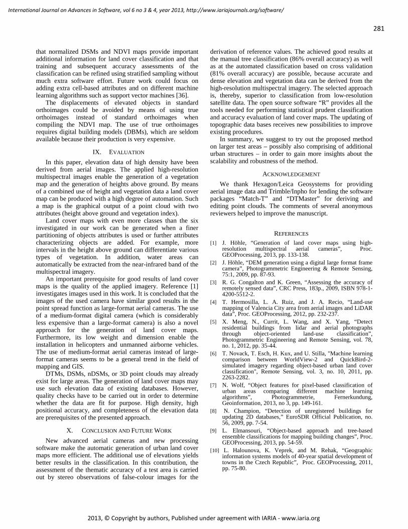
VIII. DISCUSSION The achieved overall survey weighted accuracy of the

land cover map with six classes is 86%. Regarding the important user’s accuracy, the result for class ‘building’ is correct with 99% and of class ‘road and parking lot’ with 95%. This is a very good result because simultaneously the survey adjusted producer’s accuracy for the two classes is 97% and 92%. The results for classes ‘grass’ and ‘tree’ are also good with 82% and 84% (corresponding producer’s accuracy of 82% and 76%). The derived survey weighted κ value is 0.82, which is better than the 0.76 at four classes. Using six classes improves the overall accuracy.

Automatically fitted classification trees are a computationally intensive supervised learning approach, which use more flexible splits and thresholds to perform the classification. However, these methods require a sufficiently large training set to work well. In our test example, the tree splitting rules are initially manually selected based on a-priori contextual information (e.g., a house has a certain height) and the resulting classification trees actually perform comparable to the more sophisticated machine learning approach, while being easier to interpret. One reason for this is that contextual knowledge is not captured by the purely data driven machine learning procedure - in case of small accuracy samples this makes a difference. A way to improve the automatic procedure will be to use a Bayesian framework for the classification trees where contextual information about splits is reflected as data augmented prior cases. However, when training sets are larger or contextual prior information less clear (e.g., in case of many diffuse classes or many indirect input variables), the automatic classification trees method and its refinements (e.g., classification tree ensembles) may provide superior classification results. However, our aim was not to fully explore the details of such complex classification for our test area, but rather to show

TABLE V. ERROR MATRIX OF THE DERIVED LAND COVER MAP WITH SIX CLASSES.

Class \ Reference b h g r t w row

total

building 90 0 0 0 1 0 91

hedge & bush 0 41 29 5 16 0 91

grass 1 11 75 4 0 0 91

road & parking

lot 0 1 4 86 0 0 91

tree 3 2 8 1 76 1 91

wall & car port 5 8 1 13 2 62 91

column total 99 63 117 109 95 63 546

TABLE VI. USER’S ACCURACY OF THE DERIVED LAND COVER MAP WITH SIX CLASSES

class accuracy 95% CI building 99% 95%-100%

hedge & bush 45% 35%-56% grass 82% 74%-89%

road & parking lot 95% 88%-98% tree 84% 75%-90%

wall & car port 68% 58%-77%

281



that normalized DSMs and NDVI maps provide important additional information for land cover classification and that training and subsequent accuracy assessments of the classification can be refined using stratified sampling without much extra software effort. Future work could focus on adding extra cell-based attributes and on different machine learning algorithms such as support vector machines [36].

The displacements of elevated objects in standard orthoimages could be avoided by means of using true orthoimages instead of standard orthoimages when compiling the NDVI map. The use of true orthoimages requires digital building models (DBMs), which are seldom available because their production is very expensive.

IX. EVALUATION In this paper, elevation data of high density have been

derived from aerial images. The applied high-resolution multispectral images enable the generation of a vegetation map and the generation of heights above ground. By means of a combined use of height and vegetation data a land cover map can be produced with a high degree of automation. Such a map is the graphical output of a point cloud with two attributes (height above ground and vegetation index).

Land cover maps with even more classes than the six investigated in our work can be generated when a finer partitioning of objects attributes is used or further attributes characterizing objects are added. For example, more intervals in the height above ground can differentiate various types of vegetation. In addition, water areas can automatically be extracted from the near-infrared band of the multispectral imagery.

An important prerequisite for good results of land cover maps is the quality of the applied imagery. Reference [1] investigates images used in this work. It is concluded that the images of the used camera have similar good results in the point spread function as large-format aerial cameras. The use of a medium-format digital camera (which is considerably less expensive than a large-format camera) is also a novel approach for the generation of land cover maps. Furthermore, its low weight and dimension enable the installation in helicopters and unmanned airborne vehicles. The use of medium-format aerial cameras instead of large-format cameras seems to be a general trend in the field of mapping and GIS.

DTMs, DSMs, nDSMs, or 3D point clouds may already exist for large areas. The generation of land cover maps may use such elevation data of existing databases. However, quality checks have to be carried out in order to determine whether the data are fit for purpose. High density, high positional accuracy, and completeness of the elevation data are prerequisites of the presented approach.

X. CONCLUSION AND FUTURE WORK New advanced aerial cameras and new processing

software make the automatic generation of urban land cover maps more efficient. The additional use of elevations yields better results in the classification. In this contribution, the assessment of the thematic accuracy of a test area is carried out by stereo observations of false-colour images for the

derivation of reference values. The achieved good results at the manual tree classification (86% overall accuracy) as well as at the automated classification based on cross validation (81% overall accuracy) are possible, because accurate and dense elevation and vegetation data can be derived from the high-resolution multispectral imagery. The selected approach is, thereby, superior to classification from low-resolution satellite data. The open source software “R” provides all the tools needed for performing statistical prudent classification and accuracy evaluation of land cover maps. The updating of topographic data bases receives new possibilities to improve existing procedures.

In summary, we suggest to try out the proposed method on larger test areas – possibly also comprising of additional urban structures – in order to gain more insights about the scalability and robustness of the method.

ACKNOWLEDGEMENT We thank Hexagon/Leica Geosystems for providing

aerial image data and Trimble/Inpho for lending the software packages “Match-T” and “DTMaster” for deriving and editing point clouds. The comments of several anonymous reviewers helped to improve the manuscript.

REFERENCES [1] J. Höhle, “Generation of land cover maps using high-

resolution multispectral aerial cameras”, Proc. GEOProcessing, 2013, pp. 133-138.

[2] J. Höhle, “DEM generation using a digital large format frame camera”, Photogrammetric Engineering & Remote Sensing, 75:1, 2009, pp. 87-93.

[3] R. G. Congalton and K. Green, “Assessing the accuracy of remotely sensed data”, CRC Press, 183p., 2009, ISBN 978-1-4200-5512-2.

[4] T. Hermosilla, L. A. Ruiz, and J. A. Recio, “Land-use mapping of Valencia City area from aerial images and LiDAR data”, Proc. GEOProcessing, 2012, pp. 232-237.

[5] X. Meng, N., Currit, L. Wang, and X. Yang, “Detect residential buildings from lidar and aerial photographs through object-oriented land-use classification”, Photogrammetric Engineering and Remote Sensing, vol. 78, no. 1, 2012, pp. 35-44.

[6] T. Novack, T. Esch, H. Kux, and U. Stilla, "Machine learning comparison between WorldView-2 and QuickBird-2-simulated imagery regarding object-based urban land cover classification", Remote Sensing, vol. 3, no. 10, 2011, pp. 2263-2282.

[7] N. Wolf, “Object features for pixel-based classification of urban areas comparing different machine learning algorithms”, Photogrammetrie, Fernerkundung, Geoinformation, 2013, no 3, pp. 149-161.

[8] N. Champion, “Detection of unregistered buildings for updating 2D databases,” EuroSDR Official Publication, no. 56, 2009, pp. 7-54.

[9] L. Elmansouri, “Object-based approach and tree-based ensemble classifications for mapping building changes”, Proc. GEOProcessing, 2013, pp. 54-59.

[10] L. Halounova, K. Veprek, and M. Rehak, “Geographic information systems models of 40-year spatial development of towns in the Czech Republic”, Proc. GEOProcessing, 2011, pp. 75-80.

282



[11] M. Gruber, M. Ponticelli, R. Ladstädter, and A. Wiechert, “UltraCam Eagle, details and insight”, Int. Arch. Photogramm. Remote Sens. Spatial Inf. Sci., XXXIX-B1, 2012, pp.15-19.

[12] K. Jacobsen and K. Neumann, “Property of the large-format digital aerial camera DMC II”, Int. Arch. Photogramm. Remote Sens. Spatial Inf. Sci., XXXIX-B1, 2012, pp. 21-25.

[13] R. Wagner, “The Leica RCD30 medium-format camera: imaging revolution”, Proc. Photogrammetric Week ’11, Wichmann Verlag, 2011, pp. 89-95.

[14] R Development Core Team, “R: A language and environment for statistical computing”, R Foundation for Statistical Computing, Vienna, Austria, 2013, ISBN 3-900051-07-0, http://www.r-project.org/ (accessed 10.11.2013).

[15] N.Haala, H. Hastedt, K. Wolff, C. Ressl, and S. Baltrusch, “Digital photogrammetric camera evaluation – generation of digital elevation models”, Photogrammetrie, Fernerkundung, Geoinformation, 2010, no.2, pp. 99-115.

[16] H. Hirschmüller, M. Buder, and I. Ernst, “Memory efficient semi-global matching”, ISPRS Annals of the Photogrammetry, Remote Sensing and Spatial Information Sciences, vol. I-3, 2012, pp. 371-376.

[17] T. Heuchel, “Trimble Match-T DSM“, Proc. of the EuroSDR workshop on 'High Density Image Matching for DSM Computation', EuroSDR publication nr. 61, 2012, 39 p.

[18] T. Lumley, "Survey: analysis of complex survey samples". R package version 3.28-2, http://cran.r-project.org/package=survey (accessed 10.11.2013).

[19] T. Therneau, B. Atkinson, and B. Ripley, “rpart: Recursive partitioning”, R package, version 4.1-1. http://cran.r-project.org/package=rpart (accessed10.11.2013).

[20] E. Glaab, J.M. Garibaldi, and N. Krasnogor, “vrmlgen: An R package for 3D data visualization on the Web”, Journal of statistic software, 2010, vol. 36, issue 8, pp. 1-18, http://www.jstatsoft.org/v36/i08/paper (accessed 10.11.2013).

[21] J. Cohen, “A coefficient of agreement for nominal scales”, Educational and Psychological Measurement. vol. 20, no. 1, 1960, pp. 37-40.

[22] L. D. Brown, T. T. Cai, and A. DasGupta, “Interval estimation for a binomial proportion”, Statistical Science 2001, vol. 16, no. 2, pp. 101–133.

[23] G. A. Young and R. L. Smith, “Essentials of statistical inference”, Cambridge University Press, 2005.

[24] S. Dorai-Raj, “binom: Binomial confidence intervals for several parameterizations”, R package version 1.0-5, 2009, http://cran.r-project.org/package=binom (accessed 10.11.2013).

[25] M. Höhle, “binomSamSize: Confidence intervals and sample size determination for a binomial proportion under simple random sampling and pooled sampling”, R package version 0.1-2, 2009. http://cran.r-project.org/web/packages/binomSamSize/ (accessed 10.11.2013).

[26] J. N. K. Rao and A. J. Scott, “On chi-squared tests for multiway contingency tables with cell proportions estimated from survey data”, The Annals of Statistics, vol. 12, no.1, 1984, pp. 46-60.

[27] J. Landis and G. Koch, “The measurement of observer agreement for categorical data”, Biometrics, vol. 33, 1977, pp. 159-174.

[28] S. V. Stehman, “Estimating the kappa coefficient and its variance under stratified random sampling”, Photogrammetric Engineering & Remote Sensing, vol. 62, no. 4, 1996, pp. 401-407.

[29] C-E. Särndal, B. Swensson, and J. Wretman, “Model assisted survey sampling”, Springer, 1992.

[30] G. M. Foody, “Sample size determination for image classification accuracy assessment and comparison”, International Journal of Remote Sensing, 2009, vol. 30, no. 20, pp. 5273-5291.

[31] T. Heuchel, A. Köstli, C. Lemaire, and D. Wild, “Towards a next level of quality DSM/DTM extraction with Match-T”, Proc. Photogrammetric Week ’11, Wichmann Verlag, 2011, pp. 197-202.

[32] ASRC, “LEOWorks, version 4.0,” 2011. http://leoworks.asrc.ro (accessed 10.11.2013)

[33] QGIS, “User Guide of Quantum GIS program, version 1.8.0”, 2013, 216 p., http://download.osgeo.org/qgis/doc/manual/qgis-1.8.0_user_guide_en.pdf (accessed 10.11.2013).

[34] L. Breiman, J. H. Friedman, R. A. Olshen, and C. J Stone, “Classification and regression trees”, Wadsworth, 1984.

[35] A. Peters and T. Hothorn, “ipred: Improved predictors”, R package version 0.9-1, http://cran.r-project.org/package=ipred (accessed 10.11.2013).

[36] C. Hung, L. S. Davis, and J. R. G. Townshand, “An assessment of support vector machines for land cover classification”, International Journal of Remote Sensing, 2002, vol. 23, no. 4, pp. 725–749.

Documents

Aalborg Universitet Generation and Assessment of Urban ...vbn.aau.dk/...H_hle_Generation_and_Assessment_of_Urban_Land_Cov… · Generation and Assessment of Urban Land Cover Maps