Embed Size (px)
Citation preview

ABSTRACT
Title of Document: Directed By:
A SYSTEMS RELIABILITY APPROACH TO FLOW CONTROL IN DAM SAFETY RISK ANALYSIS
Professor, Gregory Baecher, Department of Civil and Environmental Engineering
Most contemporary risk assessment techniques, such as failure modes and effect analysis
(FMEA), fault tree analysis (FTA), and probabilistic risk analysis (PRA) rely on a chain-
of-event paradigm of accident causation. Event-based techniques have some limitations
for the study of modern engineering systems; specifically hydropower dams. They are not
suited to handle complex computer-intensive systems, complex human-machine
interactions, and systems-of-systems with distributed decision-making that cut across
both physical and organizational boundaries. The emerging paradigm today, however, is
not to analyze dam systems separately by breaking the major disciplines into stand-alone
vertical analyses; but to explore the possibilities inherent in taking a systems approach to
modeling the reliability of flow-control functions within the entire system.
This dissertation reports on the development and application of systems reliability models
to operational aspects of a hydropower cascade in Northern Ontario: The Lower
Mattagami River (LMR) Project operated by Ontario Power Generation (OPG). The
reliability of flow-control systems is a broad topic that covers structural, mechanical,
electrical, control systems and subsystems reliability, as well as human interactions,

organization issues, policies and procedures. All of these occur in a broad spectrum of
environmental conditions. A systems simulation approach is presented for grappling with
these varied influences on flow-control systems in hydropower installations.
The Mattagami River cascade operated by Ontario Power Generation is a series of four
power stations along the Mattagami River and the Adams Creek bypass channel from
Little Long GS at the top to the cascade to the Mattagami River below Kipling GS at the
bottom. The number of riparians in the river flood plain is few and there is no
commercial riverine navigation, so potential loss of life is small or negligible and
operational safety dominates. The problem facing the project was to conceptualize a
systems engineering model for the operation of the dams, spillways, and other
components; then to employ the model through stochastic simulation to investigate
protocols for the safe operation of the spillway and flow control system. Details of the
modeling, analysis, and results for safe operation of the cascade are presented.
A SYSTEMS RELIABILITY APPROACH TO FLOW CONTROL IN DAM SAFETY
RISK ANALYSIS
By
Adiel Nii-Ayi Komey
Thesis submitted to the Faculty of the Graduate School of the University of Maryland, College Park, in partial fulfillment
Of the requirements for the degree of Master of Science
2014
Advisory committee:
Dr. Gregory Baecher, Chair
Dr. Lewis Ed Link
Dr. Monifa Vaughn-Cooke

© Copyright by
Adiel Nii-Ayi Komey
2014

ii
ACKNOWLEDGMENTS
First and foremost, the most heartfelt thanks go to my family (Mom, Dad, Cyril and
Rhoda) for their unconditional love and support. I would also like to thank Dr. Baecher,
my academic advisor, thesis supervisor, and friend. Your guidance, support and
enthusiasm throughout all LMR complex project at the University of Maryland made this
work possible. And last but not least, I would also like to thank my committee members
for their guidance, as well as all the members of the SSRP who generated many of the
insight upon which this research is based. Thank you to all the people at Ontario Power
Generation who provided the data and logistics and whose help with the models was
invaluable.
iii
TABLE OF CONTENTS INTRODUCTION: ON THE SYSTEMS RLIABILITY MODELING APPROACH TO RISK ANALYSIS IN DAM SAFTY 1
CHAPTER 1: RISK AND UNCERTAINTY IN DAM SAFETY-LITERATURE REVIEW 4
1.1 Understanding How Dams Fail 4
1.2 Other Factors Influencing Potential Failure in Dams 6
1.1.1 Definition of Hazard 6
1.1.2 Potential Failure Modes 9
1.1.3 Dam Life Phases 10
1.1.4 Other Factors Influencing Potential Failure in Dams 12
1.2 DAM SYSTEMS 14
1.3 CURRENT STATE OF THE PRACTICE 15
1.3.1 Standards-Based Decision-Making 16
1.3.2 Risk-informed decision making 17
1.3.3 Probabilistic risk analysis (PRA) 19
1.4 ALTERNATIVE APPROACHES 21
1.4.1 Normal Accident Theory 22
1.4.2 High Reliability Organizations 24
1.5 Systems Engineering 26
1.5.1 DAMS AS ENGINEERED SYSTEMS 26
1.6 THESIS SCOPE AND BOUNDARIES 29
1.6.1 THESIS OBJECTIVE 30
1.6.2 THESIS OUTLINE 32
CHapter 2: systems engineering application to Spillway systems 33
2.1 System Boundaries: The Context Diagram 33
2.2 STAKEHOLDER IDENTIFICATION 34
2.3 CONTEXT DIAGRAM: SPILLWAY SYSTEMS RELIABILITY ANALYSIS 35
2.4 REQUIREMENTS ANALYSIS 37
2.4.1 System Level Requirements For Proposed Analysis Framework 37
2.4.2 Allocation And Flow-Down Process 39
2.5 USE CASE DIAGRAMS 41
2.5.1 SYSTEMS LEVEL USE CASE 42
2.5.2 BUILD MODE USE CASE 43
2.5.3 Run Model Use Case 44
2.6 ACTIVITY DIAGRAMS 46
iv
2.6.3 Simulation Activity Diagram 47
Chapter 3: Lower Mattagami River Basin Case Study 49
3.1 BACKGROUND 49
3.1.1 Location 49
3.1.2 Generating Stations 51
3.1.3 Station Characteristics 52
3.2 Generating Stations 55
3.2.1 Little Long GS 55
3.2.2 Smoky Falls GS 56
3.2.3 Harmon GS 58
3.2.4 Kipling GS 60
3.3 Lower Mattagami River (LMR) Complex SYSTEMS MODELING 62
3.3.1 Current State of Events at Lower Mattagami 63
3.3.2 Existing Generating Stations 65
3.4.1 Core Objectives of the LoweR Mattagami River Case Study 66
3.4.2 Features 67
3.5 Viewpoints 67
3.6 Major Risks Identified Risks 68
3.7 SYSTEMS and Study Boundaries 68
3.8 GoldSim™ Modeling Framework 71
3.8.1 Background to GoldSim™ and the Reliability Module 71
3.8.2 THE Reliability Module 72
3.9 Why GoldSim™? 72
4. Hydrologic Modeling and Flow Routing 74
4.1 Historic Time Series Data 76
4.2 The Modeled System Schematic 78
3.3 Operating Patterns and flow routing 79
4.4 Flow Routing at Little Long 81
4.4.1 Operation (Little Long) 82
4.5 Flow Routing at Smokey Falls 84
4.5.1 Operation (Smokey) 85
3.6 Harmon Operations 85
4.7 Kipling Operations 87
4.8 Reservoir Operations Summary 87
4.8.1 Summary Spillway Operations 88
v
4.9 Power Generation 88
5.0 The Model 90
5.1 Reservoir Modeling 91
5.2 Power Generation Modeling 93
5.3 Spillway Gates and Turbine Operations 94
5.4 Modeling Local inflow at Kipling 98
5.5 Simulation Run Settings 100
5.6 Model Run Settings 101
5.7 Flow Routing Sample Results and Analysis 101
5.7.1 Pool and Volume Capacities 106
5.8 Power Production 108
6. Spillway Analysis Modeling and Reliability analysis 113
6.1 Vertical Lift Gates 113
5.3 Load Types on Gates 115
6.4 Rate of Flow and Conveyance 116
6.5 Spillway Gate Operations: Flow Routing at LMR 117
6.6 Failure 118
6.7 Failure Mechanisms 119
6.8 Failure Mode of Gates 120
6.9 Reliability and peformance of gated Spillways 122
6.9.1 Flow Routing Capacities 122
6.9.2 Modeling function and failure 122
6.10 Little Long GS Spillway Gates Modeling 124
6.11 Communication and Human Operator Modeling 124
6.13 Reservoir Operations 126
6.14 Accounting for Performance Uncertainty 127
6.14.1 Reliability of Systems 127
6.14.2 Fault Tree Analysis 128
6.14.3 Electrical and Mechanical Equipment failure and Modeling 129
5.14.4 Modeling Simple Failure Rates in GoldSim™ 129
6.14.5 Cumulative Failure Mode 130
6.14.6 The Fragility curve 131
6.14.7 Electrical Failure 133
6.15 Repair Time Distributions Used for the LMR 134
6.16 Method of Modeling : Fault tree Analysis 135
vi
6.17 BACKGROUND TO GOLDSIM™ AND THE RELIABILITY MODULE 135
6.17.1 Why Predict RAMS? 136
6.18 Modeling Little Long Spillway Reliability 137
6.19 Gate Operations AND Results Analysis 140
6.20 Gate Reliabilities 150
6.20 Disturbances 155
6.20.1 External Disturbances 156
6.20.2 Potential Environmental Conditions Likely Effects on the LMR 157
6.20.3 Modeling the Inherent disturbances 160
6.20.4 Icing effect on flow control 161
6.20.5 Modeling Ice Storms Disturbance 162
6.20.6 Modeling floating Ice 166
6.20.7 Simplified Thermal Analyses 166
7.0 SUMMARY AND CONCLUSION 169
7.1 Summary 169
7.2 CONCLUSION 170

vii
LIST OF TABLES
TABLE 1: DAM SAFETY HAZARD POTENTIAL CLASSIFICATION 7 TABLE 2: REQUIREMENTS DEFINITION TABLE ERROR! BOOKMARK NOT DEFINED.36 TABLE 3: POTENTIAL ENVIRONMENTAL CONDITIONS LMR COMPLEX 158 TABLE 4: DOWN TIMES AND REPAIR TIMES OF COMPONENT FAILURES 163 TABLE 5: STEFAN EQUATION VALUES FOR Α 167

1
INTRODUCTION: ON THE SYSTEMS RLIABILITY MODELING APPROACH TO RISK ANALYSIS IN DAM SAFTY
Each dam is unique. The site, purpose of the dam, materials available for construction,
state-of-practice when the dam was constructed, engineer’s experience and knowledge,
and many other factors combine to create structures that are as individual as people. The
consequence of failure of each dam is also unique. At one end of the spectrum are large
dams upstream of major population centers with thousands of people at risk. At the other
end are the many small dams that have little to no consequences if they were to fail. The
combination of site, design, project-specific operational requirements, and consequences
makes the risk associated with each dam unique and in most cases very complex.
Since the beginning of the industrial revolution in the late 18th century, the cause of
many serious accidents in hydropower plants has shifted from natural causes to human
and technology-related causes as these systems get more complex. While natural disasters
still account for a significant amount of human and material losses, man-made disasters
are responsible for an increasingly large portion of the toll, especially in a safety critical
domain such as hydropower generation. The reliable performance of a hydraulic flow-
control system such as dams, reservoirs, etc. depends on the time-varying demands
placed upon it by hydrology, operating rules, the interactions among a cascade of
reservoirs, the vagaries of operator interventions and natural disturbances (Baecher,
2014). In the past, engineers have concerned themselves with understanding how the
component parts of dam systems operate individually and not how the components
interact with one another. Dams and their associated flow control are highly complex
systems of engineered structures, natural processes, and human operation. They behave in
2
complex ways that are not amenable to such simple decompositional analysis, and thus
need to be understood in a systems engineering context.
Contemporary engineering practices do not address many common causes of accidents
and failures, which are unforeseen combinations of usual conditions. In recent decades,
the most likely causes of fatalities associated with dams have more often had to do with
sensor and control systems, human agency, and inadequate maintenance than with
extreme loads such as floods and earthquakes. Research on dam failures and safety
related incidents has shown that most dam failures were not caused by a single, easily
analyzed, component failure but rather by interactions between various components and
subsystems. To throw more light on this, Accidents and failures usually occur due to the
un-foreseen confluence of more common and individually benign events, which in
combination can be catastrophic(Baecher, 2014).
A “new approach” was proposed which combines simulation, engineering reliability
modeling, and systems engineering. This new approach seeks to explore the possibilities
inherent in taking a systems approach to modeling the reliability of flow-control
functions and dam systems. The approach takes into account interconnections and
dependences between different components of the system, changes over time in their
state as well as the influence upon the system of organizational limitations, human errors
and external disturbances. The method attempts to bring together the systems aspects of
engineering and operational concerns in a way that emphasizes their interactions.
On-going research by the Spillway Systems Reliability Project (SSRP) on this proposed
systems engineering approach has been a complex multi-year effort entirely coded in
matlab. However, with the recent proliferation of third party Simulation engines better
3
optimized for engineering reliability modeling such as GoldSim™ and RENO™, there was
a need to test these platforms to investigate whether it offers an overall better program
interface and customizability than the Mat lab platform.
The research centers on the use of GoldSim™ Simulation engine and its extensions to
model at component and subcomponent level, the reliable performance of the entire dam
system. The modeling approach holistically integrates river basin hydrology, the routing
of reservoir inflows through the reservoir system, operating rules and human factors of
operating the spillway and other waterways, out flow systems, the hydraulics of outflow,
the discharge to the downstream river channel and the fragility of the structural,
mechanical and electrical components of the dam system. Emphasis is placed on the
interactions of this set of components and how unforeseen combinations of varying
conditions may lead to failure of dam system. The Lowe Mattagami River Hydroelectric
complex is used as a case study for this research. The present goal of this study is to
understand how the interactions of systems components and subcomponents, control and
combine to affect performance, and the potential for accidents and failures; thus, how
simple but unforeseen chains of events might combine to affect the ability to control
flows.
The final objective of this dissertation is to incorporate all the different aspects of dams
operations into a single systems model which can be broken down and analyzed at the
component and subcomponent level. In order to achieve this objective, it is necessary to
identify and model the dynamic feedback processes that may cause risk to increase over
time into the overall model. This dissertation introduces a systems framework to model
some critical aspects of safety and power generation in dam systems.
4
CHAPTER 1: RISK AND UNCERTAINTY IN DAM SAFETY-LITERATURE
REVIEW
1.1 UNDERSTANDING HOW DAMS FAIL
A dam is a barrier that impounds water or underground streams. Dams generally serve
the primary purpose of retaining water. Dams are built for many purposes including
power supply, transportation, water supply, flood control, recreation, industrial and
agricultural uses, fire protection, low flow augmentation, storage of slurries, storage of
tailings and storage of industrial wastes. Dams can be made of concrete, timber cribs
filled with rocks, stone blocks, steel sheet piling, or they can be formed from
embankments of earth, rock fill or solid waste products such as tailings. While other
structures such as floodgates or levees (also known as dikes) are used to manage or
prevent water flow into specific land regions. Hydropower and pumped-storage
hydroelectricity are often used in conjunction with dams to generate electricity. Types of
dams include water storage reservoirs, locks, weirs, mine tailings dams, and levees.
Dam failure is the uncontrolled release of impounded water or other stored material
resulting in downstream flooding, which can affect life and property. Dams can fail with
little warning. Intense storms may produce a flood in a few hours or even minutes for
upstream locations. Flash floods can occur within six hours of the beginning of heavy
rainfall, and dam failure may occur within hours of the first signs of breaching. Other
failures and breaches can take much longer to occur, from days to weeks, as a result of
debris jams, the accumulation of melting snow, buildup of water pressure on a dam with
(unknown) deficiencies after days of heavy rain, etc. Flooding can also occur when a dam
operator releases excess water downstream to relieve pressure from the dam. Proper

5
attention to dam safety is vital to protect downstream life, property and habitat. Safety
concerns include sinkholes, seepage, internal erosion and seismic issues.
The consequences of a dam failure can vary from none to major. For example a minor
overtopping that is remedied quickly has low consequences. Without immediate
attention, the dam may further erode, leading to a complete breach and major
consequences in many ways. Some potential consequences include the following:
• Loss of life;
• Damage to homes, businesses, transportation networks, lifelines, utilities, schools
industrial facilities and other improvements;
• Damage to the environment;
• Threat to other dams located downstream that can result in cascade failures;
• Loss of stored materials;
• Loss of use of the dam;
• Loss of economic benefit from the dam;
• Loss of the capital investment to the dam’s owner;
• Fines to the owner;
• Criminal charges to owner or designer;
• Lawsuits and other litigation;
• Destruction of the owner’s business; and
• Damage to reputation of owner, design engineer and regulator.
6
1.2 OTHER FACTORS INFLUENCING POTENTIAL FAILURE IN DAMS
An examination of dam failures and safety related incidents shows that most were not
caused by a single, easily analyzed, component failure but rather by interactions between
various components, operational considerations, and lack of appropriate organizational
response (Paul C. Rizzo Associates, Inc., 2007). It is imperative to reduce the risk
associated with a dam to a level that is as low as reasonably practicable. The optimum
must done within the associated operating constraints and within the limits of current
knowledge and understanding, to recognize potential failure modes before they begin to
develop and to monitor those failure modes over time. To achieve this goal, dam owners
must find an effective way to integrate operations, engineering, and dam safety
performance monitoring into a comprehensive dam safety program. Performance
monitoring and record keeping are essential to making well-informed decisions regarding
the condition of the dam. As the systems that control dams get more complex and more
automated, and more are remotely operated, opportunities increase for undetected
incidents that can lead to dam failure. Understanding factors relating to dam safety, such
as owner risk awareness, management responsibility, personnel training, and system and
sub-system interactions, are become increasingly important.
1.1.1 DEFINITION OF HAZARD
Dam failures and incidents of most concern involve unintended or uncontrolled releases
or surges of impounded water. It may also involve a total collapse of the dam but that is
not always the case (Paul C. Rizzo Associates, Inc., 2013). Damaged spillways,
7
overtopping of a dam or other problems may result in a hazardous situation being created.
In some cases, it is an unintended consequence of the dam’s operations.
During the last 40 to 50 years, the general understanding of how dams fail has progressed
sufficiently to provide guidance for dam engineers and builders to help prevent similar
failures. Lessons learned were codified and design practices standardized. However,
dams continue to fail. Forensic examinations of recent dam failures often reveal that
failures were not due to a single flaw but rather were due to a complex linking of dam
condition, operational circumstances, flaws or errors that combined to result in failure, or
unknowns that were not detected until after the failure. This linkage of “conditions” and
“other factors” is one possible description of a “failure mode.”
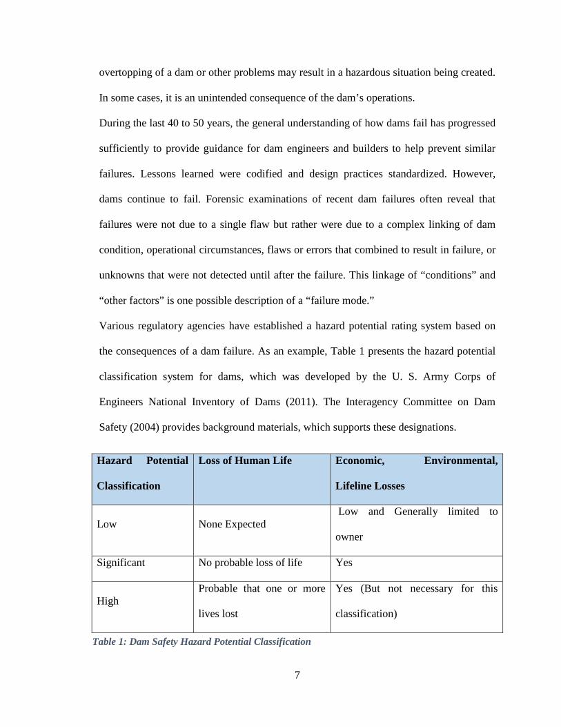
Various regulatory agencies have established a hazard potential rating system based on
the consequences of a dam failure. As an example, Table 1 presents the hazard potential
classification system for dams, which was developed by the U. S. Army Corps of
Engineers National Inventory of Dams (2011). The Interagency Committee on Dam
Safety (2004) provides background materials, which supports these designations.
Hazard Potential
Classification
Loss of Human Life Economic, Environmental,
Lifeline Losses
Low None Expected Low and Generally limited to
owner
Significant No probable loss of life Yes
High Probable that one or more
lives lost
Yes (But not necessary for this
classification)
Table 1: Dam Safety Hazard Potential Classification
8
Loss of human life potential is based upon inundation mapping of the area downstream of
the project. Analysis of loss of life potential should take into account the population at
risk, time of flood wave travel and wave height, and warning time. Indirect threats to life
caused by the interruption of lifeline services due to dam failure or operation, i.e. direct
loss of critical medical facilities, should also be considered. Economic, environmental,
and lifeline impacts should be evaluated based on the incremental flood wave produced
by dam failure, beyond which would normally be expected for the magnitude of the flood
event which the failure occurs.
Typical dam hazard potential classifications can vary with regulatory jurisdiction; Hazard
potential classification can be described more generally as follows.
Low Hazard Potential dams are located in areas where failure will damage nothing
more than isolated buildings, undeveloped lands, or town or county roads and/or will
cause no substantial economic loss or substantial environmental damage. Loss of human
life is not expected.
Economic, environmental, and lifeline impacts are considered to be low and generally
limited to the owner.
Significant Hazard Potential dams are located in areas where failure may damage
isolated homes, main highways and minor railroads, interrupt the use of relatively
important public utilities and/or will cause substantial economic loss or substantial
environmental damage.
High Hazard Potential dams are located in areas where failure may cause loss of human
life, substantial damage to homes, industrial or commercial buildings, important public
9
utilities, main highways or railroads and/or will cause extensive economic or
environmental losses.
In addition to its hazard potential, a dam may exist in different performance states. Many
dams operate in very safe and well defined conditions. Others may have problems that
require more attention and response. Three performance states are used in this document
to help define the scope of a dam safety monitoring program.
Normal – performance is within the design parameters with no anomalous behavior and
no indicators of undesirable performance and is expected to remain in this state for the
near future.
Caution – performance is outside the range expected in the design, or anomalous
behavior not anticipated in the design is occurring, or an indicator of undesirable
performance is occurring at an increasing rate.
Alert – performance is in a range where safety of the dam is in question, or performance
is deteriorating and not controllable (Paul C. Rizzo Associates, Inc., 2013).
1.1.2 POTENTIAL FAILURE MODES
A potential failure mode is any means by which any component of a dam may fail to
perform its intended function. Understanding potential failure modes for dams is the basis
of a good dam safety program (Regan et al., 2008; USSD, 2002).
Dam failures may be caused by structural deficiencies in the dam itself. These may come
from poor initial design or construction, lack of maintenance and repair, the gradual
weakening of the dam through the normal aging processes, or the development of an
unanticipated or undetected failure condition. However, they can also be caused by other

10
factors including, but not limited to, debris blocking the spillway, flooding, earthquakes,
volcanic lava flows, landslides, improper operation, vandalism, or terrorism (Paul C.
Rizzo Associates, Inc., 2013).
Dam failures can result from any one or a combination of the following conditions:
• Prolonged periods of rainfall and flooding, which cause most failures;
• Inadequate spillway capacity, resulting in overtopping of the embankment;
• Internal erosion caused by loss of soil from the interior of the dam or its foundation;
animal burrow impacts on earthen dams;
• External erosion due to lack of maintenance;
• Improper maintenance, including failure to remove trees, repair internal seepage
problems, or maintain gates, valves, and other operational components;
• Improper design or use of construction materials;
• Failure of upstream dams in the same drainage basin;
• Landslides into reservoirs, which cause surges that result in substantial erosion or
overtopping;
• Destructive acts of terrorists; and,
• Earthquakes, which typically cause longitudinal cracks at the tops of the embankments,
leading to structural failure.
1.1.3 DAM LIFE PHASES
USSD (2008) describes the life of a dam as having several distinct phases. Performance
monitoring needs vary depending on which phase the dam is in. Dam life phases can be
categorized as:
11
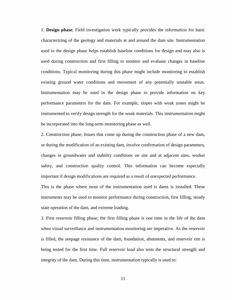
1. Design phase; Field investigation work typically provides the information for basic
characterizing of the geology and materials at and around the dam site. Instrumentation
used in the design phase helps establish baseline conditions for design and may also is
used during construction and first filling to monitor and evaluate changes in baseline
conditions. Typical monitoring during this phase might include monitoring to establish
existing ground water conditions and movement of any potentially unstable areas.
Instrumentation may be used in the design phase to provide information on key
performance parameters for the dam. For example, slopes with weak zones might be
instrumented to verify design strength for the weak materials. This instrumentation might
be incorporated into the long-term monitoring phase as well.
2. Construction phase; Issues that come up during the construction phase of a new dam,
or during the modification of an existing dam, involve confirmation of design parameters,
changes in groundwater and stability conditions on site and at adjacent sites, worker
safety, and construction quality control. This information can become especially
important if design modifications are required as a result of unexpected performance.
This is the phase where most of the instrumentation used is dams is installed. These
instruments may be used to monitor performance during construction, first filling, steady
state operation of the dam, and extreme loading.
3. First reservoir filling phase; the first filling phase is one time in the life of the dam
when visual surveillance and instrumentation monitoring are imperative. As the reservoir
is filled, the seepage resistance of the dam, foundation, abutments, and reservoir rim is
being tested for the first time. Full reservoir load also tests the structural strength and
integrity of the dam. During this time, instrumentation typically is used to:
12
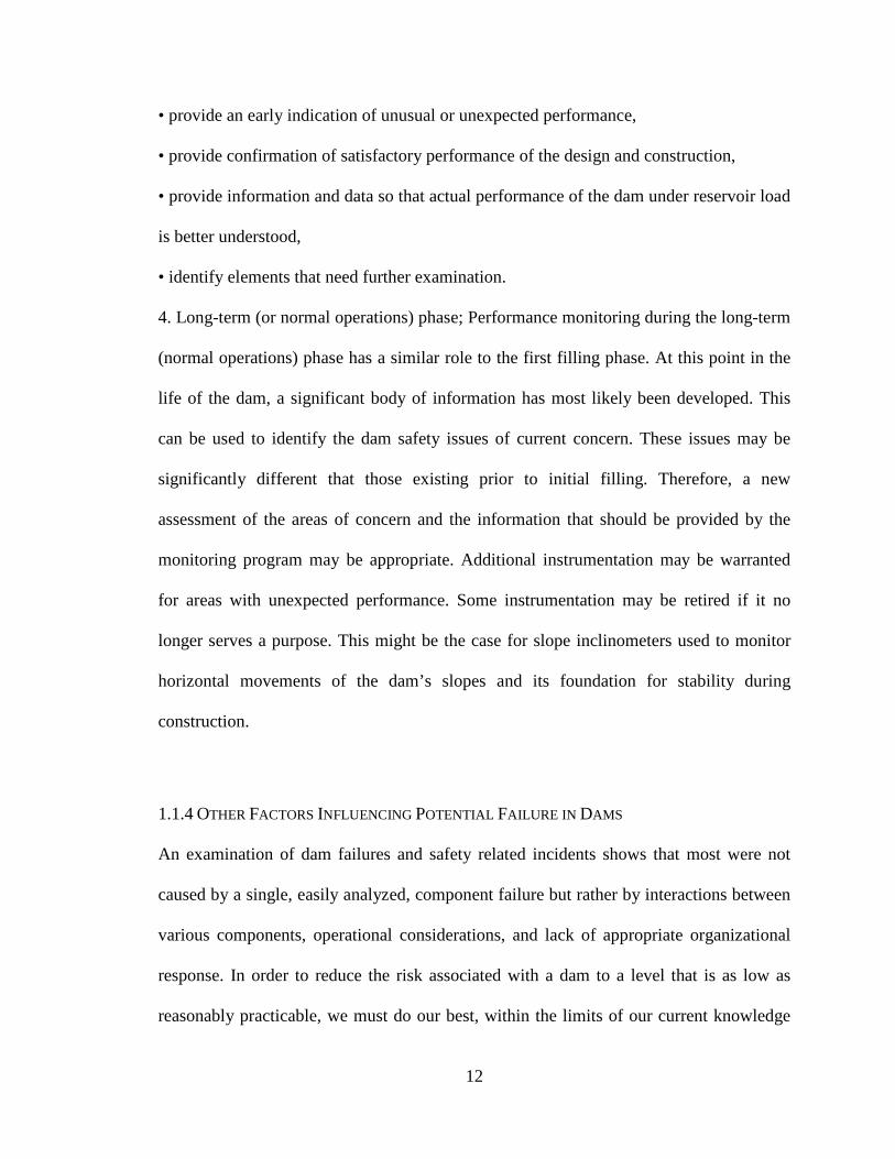
• provide an early indication of unusual or unexpected performance,
• provide confirmation of satisfactory performance of the design and construction,
• provide information and data so that actual performance of the dam under reservoir load
is better understood,
• identify elements that need further examination.
4. Long-term (or normal operations) phase; Performance monitoring during the long-term
(normal operations) phase has a similar role to the first filling phase. At this point in the
life of the dam, a significant body of information has most likely been developed. This
can be used to identify the dam safety issues of current concern. These issues may be
significantly different that those existing prior to initial filling. Therefore, a new
assessment of the areas of concern and the information that should be provided by the
monitoring program may be appropriate. Additional instrumentation may be warranted
for areas with unexpected performance. Some instrumentation may be retired if it no
longer serves a purpose. This might be the case for slope inclinometers used to monitor
horizontal movements of the dam’s slopes and its foundation for stability during
construction.
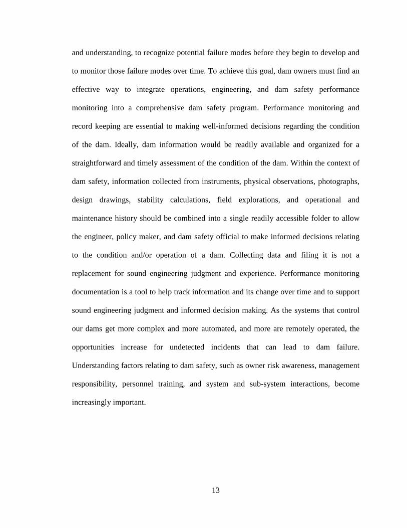
1.1.4 OTHER FACTORS INFLUENCING POTENTIAL FAILURE IN DAMS
An examination of dam failures and safety related incidents shows that most were not
caused by a single, easily analyzed, component failure but rather by interactions between
various components, operational considerations, and lack of appropriate organizational
response. In order to reduce the risk associated with a dam to a level that is as low as
reasonably practicable, we must do our best, within the limits of our current knowledge
13
and understanding, to recognize potential failure modes before they begin to develop and
to monitor those failure modes over time. To achieve this goal, dam owners must find an
effective way to integrate operations, engineering, and dam safety performance
monitoring into a comprehensive dam safety program. Performance monitoring and
record keeping are essential to making well-informed decisions regarding the condition
of the dam. Ideally, dam information would be readily available and organized for a
straightforward and timely assessment of the condition of the dam. Within the context of
dam safety, information collected from instruments, physical observations, photographs,
design drawings, stability calculations, field explorations, and operational and
maintenance history should be combined into a single readily accessible folder to allow
the engineer, policy maker, and dam safety official to make informed decisions relating
to the condition and/or operation of a dam. Collecting data and filing it is not a
replacement for sound engineering judgment and experience. Performance monitoring
documentation is a tool to help track information and its change over time and to support
sound engineering judgment and informed decision making. As the systems that control
our dams get more complex and more automated, and more are remotely operated, the
opportunities increase for undetected incidents that can lead to dam failure.
Understanding factors relating to dam safety, such as owner risk awareness, management
responsibility, personnel training, and system and sub-system interactions, become
increasingly important.
14
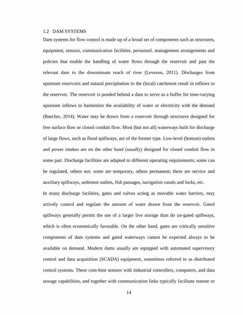
1.2 DAM SYSTEMS
Dam systems for flow control is made up of a broad set of components such as structures,
equipment, sensors, communication facilities, personnel, management arrangements and
policies that enable the handling of water flows through the reservoir and past the
relevant dam to the downstream reach of river (Leveson, 2011). Discharges from
upstream reservoirs and natural precipitation in the (local) catchment result in inflows to
the reservoir. The reservoir is ponded behind a dam to serve as a buffer for time-varying
upstream inflows to harmonize the availability of water or electricity with the demand
(Baecher, 2014). Water may be drawn from a reservoir through structures designed for
free surface flow or closed conduit flow. Most (but not all) waterways built for discharge
of large flows, such as flood spillways, are of the former type. Low-level (bottom) outlets
and power intakes are on the other hand (usually) designed for closed conduit flow in
some part. Discharge facilities are adapted to different operating requirements; some can
be regulated, others not; some are temporary, others permanent; there are service and
auxiliary spillways, sediment outlets, fish passages, navigation canals and locks, etc.
In many discharge facilities, gates and valves acting as movable water barriers, may
actively control and regulate the amount of water drawn from the reservoir. Gated
spillways generally permit the use of a larger live storage than do un-gated spillways,
which is often economically favorable. On the other hand, gates are critically sensitive
components of dam systems and gated waterways cannot be expected always to be
available on demand. Modern dams usually are equipped with automated supervisory
control and data acquisition (SCADA) equipment, sometimes referred to as distributed
control systems. These com-bine sensors with industrial controllers, computers, and data
storage capabilities, and together with communication links typically facilitate remote or
15
even automatic control of components of the flow-control system. The consequences of
failure of SCADA systems can be dramatic. As a result, hardware and software for
SCADA systems in dam and reservoir operations are usually ruggedized to withstand
temperature, vibration, and voltage extremes, and are enhanced by having redundant
hardware and communications capabilities. Programming errors and component failures
may still incapacitate SCADA systems. SCADA systems provide for human operator
control, both remote control from dispatch centres and local on-site control. Operators are
always important in dam operations, including flow control. As a result, also human
operators may cause mistakes or introduce errors of commission or omission into
operation of dam systems, either without intent or, less commonly, out of malice. Human
operators may also take actions that may be, or that they believe to be, in concert with
operating policy, yet which may lead to mal-operation.
The combination of electrical generators and hydraulic turbines allows hydropower
systems to convert the potential energy of dammed or flowing water into storable
electrical output. Although this conversion relies on relatively simple mechanical
properties, the system employed to achieve it is often complex in its design and
capabilities.
1.3 CURRENT STATE OF THE PRACTICE
Contemporary dam safety decision-making generally falls into one or more of the
following categories:
• Standards-based decision making,
• Risk-informed decision making, or
16
• Probabilistic risk analysis.
1.3.1 STANDARDS-BASED DECISION-MAKING
By definition, a standards-based system provides a specific standard, factor of safety,
against which the result of an analysis is measured. Standards-based decisions are
essentially decisions based on engineering principles and norms that employ a form of
design checking against stated criteria. Standards have been developed over many years
in an attempt to cover favorable performance and avoid unfavorable performance.
Typical standards-based decision-making is well exemplified by many state and federal
dam safety guidelines where sections are devoted to determining the Probable Maximum
Flood (PMF); selecting the Inflow Design Flood (IDF); and analyzing concrete gravity,
embankment and arch dams against defined factors of safety for three loading conditions
(normal, flood and seismic), etc (Regan, 2010).
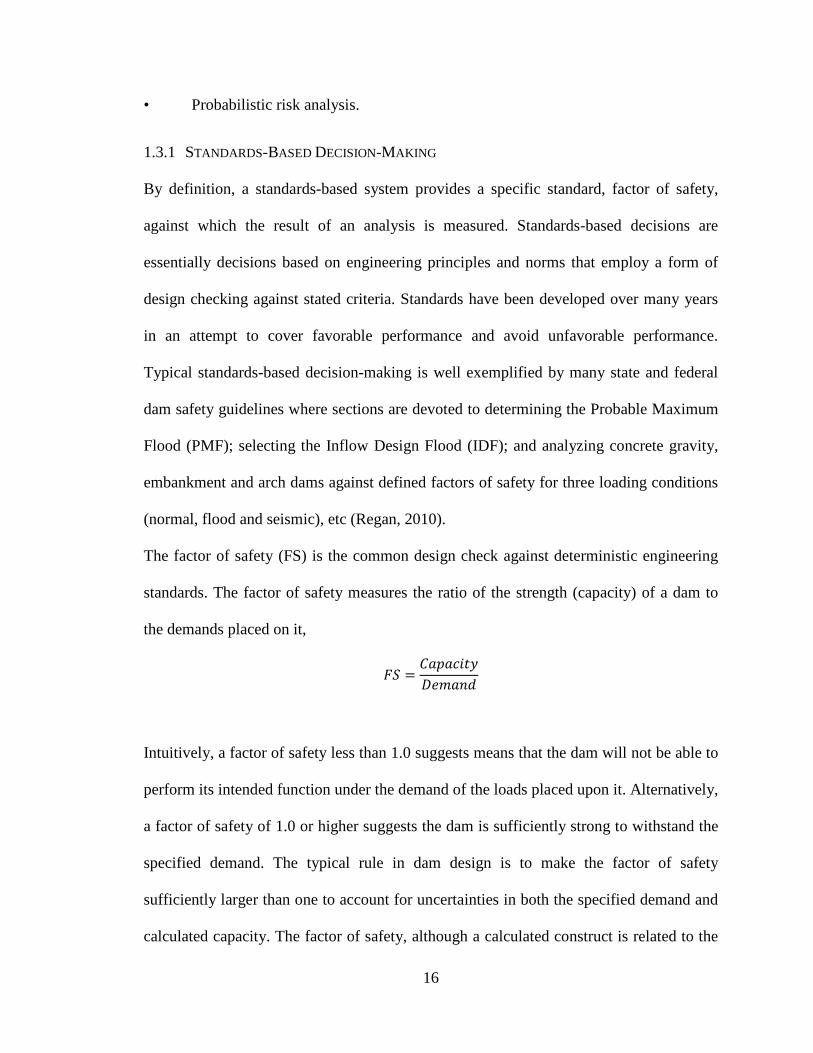
The factor of safety (FS) is the common design check against deterministic engineering
standards. The factor of safety measures the ratio of the strength (capacity) of a dam to
the demands placed on it,
�� � �������� ���
Intuitively, a factor of safety less than 1.0 suggests means that the dam will not be able to
perform its intended function under the demand of the loads placed upon it. Alternatively,
a factor of safety of 1.0 or higher suggests the dam is sufficiently strong to withstand the
specified demand. The typical rule in dam design is to make the factor of safety
sufficiently larger than one to account for uncertainties in both the specified demand and
calculated capacity. The factor of safety, although a calculated construct is related to the
17
physical properties of a dam, in that the larger the factor of safety, the greater the capacity
of the dam to with-stand the applied loads.
Quantitative engineering standards are usually promulgated by regulatory authorities,
even though they are typically taken from industry practices, by standards-setting
professional organizations approved by government; by the industry; or more indirectly
in terms of guidance provided by non-governmental organizations such as the national
member bodies of ICOLD (Baecher, 2014). Current dam safety practice is usually
predicated on the rare occurrences of extreme loads, such as unlikely but possible
reservoir inflows or powerful seismic events.
Engineering standards based decision making has evolved over the years but it’s focus
still remains on the physical structure, not on operations, data collection, communications
or operations(Baecher, 2014). Loading scenarios are assessed separately: meaning the
capacity of spillways and other waterways is considered to the extent that they are large
enough and stable enough to accommodate specified discharges; the mechanical and
electrical performance of gates and valves are considered to the extent of their
availability on demand. Analytical criteria for the internal erosion of embankment dams
have improved somewhat since that era, but still today, operational factors, SCADA
system errors, and human factors have little place in engineering-standards based
assessment of dam safety(Baecher, 2014).
1.3.2 RISK-INFORMED DECISION MAKING
Risk-informed dam safety programs provide many benefits. However, according to
Baecher et al, “Risk-informed decision making is different from engineering standards-

18
based decision making in that the focus is on the level of protection to the public from the
hazardous dam and reservoir.” In contrast, in standards-based decision making the
hazards are the natural and other conditions that threaten the dam. What generally passes
for a risk-informed approach might more accurately be described as traditional standards-
based rational with a probabilistic outlook.
Risk-informed decision-making implies taking into consideration a probabilistic
description of the natural and other hazards imposed on, and the fragility of, the dam
system, as well as the quantitative consequences of accidents or failures, in making
decisions about dam safety, in a way that is focused on the totality of the level of
protection to the public (Baecher, 2014). Within this context, risk is taken to be the
expected consequences of accidents or failures, that is, the product of the probability of
an accident or failure, and the resultant consequences of that accident or failure. Risk-
informed decision making involves balancing the expected economic, social, and
environmental costs of a dam safety risk against the costs of risk reduction, at least in a
qualitative way.
The shortcomings of this approach is its inability to assess non-linear failure modes and
interactions between apparently unrelated components and subsystems. This hinders the
identification of opportunities to prevent failures before they progress to the point where
a typical risk analysis would begin (Regan, 2010). This linear nature of typical risk
assessment approaches, combined with the fact that the majority of dam safety
professionals are civil engineers, results in a rather narrow focus on failure modes that
affect the civil structures and a neglect of the contributions to those failure modes from
electrical, mechanical and control systems or human decision-making.
19
1.3.3 PROBABILISTIC RISK ANALYSIS (PRA)
Probabilistic risk assessment (PRA) provides practical techniques for predicting and
managing risks (i.e., frequencies and severities of adverse consequences) in many
complex engineered systems.
Risk-based decision making differs from risk-informed decision making in that it relies
on the quantitative evaluation of the probabilities of accidents and failures, and of their
corresponding consequences, in order to calculate quantitative risk. In the literatures of
techno-logical risk management, risk-based decision making is often referred to as
probabilistic risk analysis (PRA). The principal methodologies of PRA are fault-tree and
event-tree analysis. The former is more common in nuclear and chemical plant safety.
The latter is more common in dam safety and civil infrastructure risk analysis.
Fault tree analysis (FTA) is a technique whose mathematical foundation is well-
developed and that has been applied extensively in reliability and safety assessments for a
wide range of engineered systems such as missile launch systems, chemical process
facilities, nuclear power plants, dams, control systems and computers. In addition, the
software and the databases available for conducting a FTA are sophisticated and add
significantly to the efficiency of performing a risk analysis. The fault tree is a graphical
construct that shows the logical interaction among the elements of a system whose failure
individually or in combination could contribute to the occurrence of a defined undesired
event such as a system failure. Fault trees offer the analyst the capability to construct a
logic model of a system that is visual and therefore is easy to view and read, and that
provides a qualitative and quantitative insight to the system’s operations and reliability.
20
It is important to note at the outset that FTA is one of many tools available to the risk
analysis team. In a risk analysis for a dam system, various methods will generally be used
to build a logic structure to analyze the expected future performance. As such, FTA will
simply be one of the methods used. In the course of the risk assessment it is important to
co-ordinate how a FTA for a system fits into the overall risk analysis model. This theme
is critical to the risk analysis in general and to the FTA in particular.
Event tree analysis (ETA) is one of the techniques available to the engineer conducting a
reliability or safety analysis for a dam. It is an apparently straightforward endeavor that
finds widespread application in many industries and businesses. It is an inductive type of
analysis that, unlike fault tree analysis, is not supported by an extensive theoretical basis.
ETA is the most widely used form of analysis in risk analysis for dam safety, although
the lack of theoretical basis means that the correctness of these constructs may be
difficult to determine.
An ETA is an analysis process whose essential component is the event tree. The event
tree is a graphical construct that shows the logical sequence of the occurrence of events
that is visual and therefore is easy to view and read, and that provides a qualitative and
quantitative insight to the system’s operations and reliability.
Current dam safety practice, both in the traditional deterministic form and in the more
modern probabilistic risk analysis (PRA) form using fault trees and event trees, is still
usually based on the rare occurrences of extreme loads, such as unlikely but possible
reservoir inflows or powerful seismic events. Adding PRA to the evaluation changes this
situation not at all. As an example, the Canadian Dam Association (CDA) guidelines for
dam safety risk analysis presume extreme floods and earthquakes to be probabilistically

21
independent events. Each has some probability of occurring in any given year, and each
has some probability of leading to an accident or failure. This is the same whether in
standards-based evaluation or in PRA. Indeed, from a geophysical view, these natural
phenomena likely are probabilistically independent. The occurrence of one does nothing
to change the probability of occurrence of the other.
From an operational and safety view, however, earthquakes and floods are not
independent. If an earthquake occurs and causes serious damage to a dam system, it may
take a year or more for repairs to be completed.
1.4 ALTERNATIVE APPROACHES
A dam is not a single independent entity but rather its system comprising of the dam body
and the waterways past the dam, usually with accompanying mechanical and electrical
equipment for on-site operational control. A dam may also be considered to include the
reservoir, communication links, and the organization responsible for operation of the
system, including on-site operators, dispatch center and company policy makers. This
system is made up of several subsystems for instance the spillway subsystem will include
the gates and its complete hoist and control system, the spillway chute and the stilling
basin. Thus the dam system would include all the subsystems that we normally associate
with a dam: i.e., the foundation, abutments, reservoir, and reservoir rim, the operating
organization and may also include a powerhouse and all its associated subsystems.
The state and nature of these components and sub components will not remain constant
during the lifetime of a dam system for reasons such as wear and aging and maintenance
activities as well as changes to the surrounding infra-structure and society. On a larger

22
scale, a dam might be a subsystem within a larger system that could be a watershed with
projects owned by one or more entities or an entire regional electrical grid.
1.4.1 NORMAL ACCIDENT THEORY
This concept was developed by Charles Perrow in his book Normal Accidents (1984), in
which he uses the term normal accidents in part as a synonym for “inevitable accidents.”
This categorization is based on a combination of features of such systems: interactive
complexity and tight coupling. Normal accidents in a particular system may be common
or rare, but the system's characteristics make it inherently vulnerable to such accidents,
hence their description as “normal”.
NAT suggests that high risk systems have some special characteristics including complex
interactions, dependencies and performance conditions that make it essentially impossible
to foresee all possible failures, especially when one “minor” failure interacts with one or
more other “minor” failures in an unforeseen manner. Since the failure of some parts is
unavoidable, some failures must be expected and should be considered “Normal”. Perrow
advocates a focus on the overall system rather than individual components. Failure in just
one part (material, sub-system, human, or organization) may coincide with the failure of
an entirely different part, revealing hidden connections, neutralized redundancies, random
occurrences etc., for which no engineer or manager could reasonably plan.
Historically dams were operated by dam operators residing near the dam and working
almost exclusively to assure the safe and reliable operation of the dam. Economic and
Socio-political pressures, brought about in large part by deregulation of the electric
industry, have resulted in the conversion of dam operations from a local dam tender to a
23
remote operations control center (Regan, 2010). Thus, human operators on site have been
consequently replaced with SCADA (Supervision, Control and Data Acquisition) which
is composed of but not limited to river gauges upstream of the reservoir, gauges within
the reservoir and gauges at the spillway. At the control center one or more operators (no
longer dam tenders) make decisions on dam operations based on information obtained
from SCADA systems without directly seeing the structure. In addition, an operator’s
principal responsibilities are often primarily related to operation of one or more
powerhouses with dam safety as an additional responsibility (Regan, 2010).
Likewise, spillway gates are now rarely operated by a dam operator on site. Presently, a
remote operator may click a virtual button on a computer screen. In the first case, the dam
tender gets immediate visual feedback that the proper gate is indeed moving or not. In the
second case, the remote operator gets a signal that the gate is moving from some form of
position sensor. If the sensor is giving erroneous data, the operator has no real knowledge
if the gate is moving or how far it is moving (Regan, 2010).
When we bring the causes of technological accidents up to closer scrutiny in a bid to
understand them the inherent causes, it’s often very difficult to pinpoint what exactly
went wrong. The reason for this is that technologies are intrinsically complex and depend
on many things working closely together: Materials and components of different quality
are structured into tightly engineered sub-systems, which are operated by error-prone
humans in not always optimal organizational structures, which in turn are subject to
production pressures and all kinds of managerial maneuvering.

24
Normal Accidents was first published in 1984, prior to the deregulation of the electric
industry and prior to the large-scale introduction of remote operation of dams. These two
factors Dams as Systems have greatly increased the complexity of dam operation and
have introduced opportunities for unforeseen interactions that did not previously exist.
Therefore, the author believes that dams today would more properly be plotted between
power grids (as plotted by Perrow in 1984) and nuclear power plants in the upper right
quadrant.
Charles Perrow, the author of Normal Accident Theory, came to the conclusion that
“some technologies, such as nuclear power, should simply be abandoned because they are
not worth the risk.” This political statement has made Normal Accident Theory highly
controversial, and the main body of research has since then concentrated on how to make
organizations and high-risk technologies more reliable, i.e. 'disaster proof', so that the
political and democratically important discussion of allowing or not allowing specific
technologies not needs to be taken.
1.4.2 HIGH RELIABILITY ORGANIZATIONS
Subsequent researchers challenged Perrow’s theory, and in particular his conclusions
regarding the inevitability of accidents. Another school of thought, High Reliability
Organizations (HRO), argues that four key organizational characteristics: 1) prioritization
of safety and performance and achieving a consensus on the goals throughout the
organization; 2) promoting a culture of reliability; 3) organizational learning to learn
from accidents and safety related incidents; and 4) use of redundancy. Advocates of HRO
suggest that by improving the reliability of components, system safety can be improved.
25
Critics of the HRO theory point out that simultaneously promoting safety and
performance, i.e. dam safety and powerhouse generation creates conflicting priorities.
HRO describes a subset of hazardous organizations that enjoy a high level of safety over
long periods of time. What distinguishes types of high-risk systems is the source of risk,
whether it is the technical or social factors that the system must control or whether the
environment, itself, constantly changes. Promoting reliability is often taken to mean
training all employees on exactly the steps to take in a safety related incident.
Unfortunately, this can mean, at times, that the employees do exactly what they’ve been
trained to do but the specific incident was outside the understanding of those who
prepared the training and the response actually hastens the incident due to unforeseen
interactions. Learning from our past clearly has its place in any dam safety program but
this is due mainly to the fact that our industry has historically evolved at a relatively slow
rate. The recent development of SCADA systems that allow remote operation of dams is
a radical departure from the historical developments in dam design and operation. We
have little to no history to help us understand the risks inherent in remote operation of
dams. It is notable that many of our recent experiences with uncontrolled releases of
water are due to unintended operation of outlet works by glitches in SCADA systems, an
area where the dam safety community has relatively little history. The last concern with
HRO is its emphasis on redundancy, a fact that may increase complexity and thereby
reduce safety, especially if operations become complacent because redundancy is
designed in.
26
1.5 SYSTEMS ENGINEERING
Another school of thought that has gathered momentum due to the advances made in
computing power over the last 3 decades is the Systems Engineering approach. Systems
theory dates back to the 1930’s and 1940’s and was a response to the limitations of the
classical analysis techniques in coping with increasingly complex systems starting to be
built at that time (Leveson, 2011). Bell Telephone laboratories developed systems
engineering in the 1940s as a response to the need to evaluate the properties of a system
as a whole, which in complex technologies, can be very different from the sum of the
properties of the individual component properties. Systems engineering advocates a high
level, top-down, view of the system and the relationships between technical,
organizational and social aspects. Systems engineering is a multi-disciplinary approach
that enables the successful realization and deployment of systems, however simple or
complex they may be. The systems approach to assessing the performance and safety of
dams is familiar from the perspective of dam design, and yet unfamiliar from the
perspective of dam safety assessment (Baecher, 2014).
1.5.1 DAMS AS ENGINEERED SYSTEMS
Safety approaches based on systems theory consider accidents as arising from the
interactions among system components. This systems approach treats safety as an
emergent property that arises when the system components interact within an
environment. Dams are engineered systems that are set in a natural environment, as such,
the dam system comprising the dam and appurtenant structures, reservoir, foundations,
abutments etc. is an engineering altered natural system(Baecher & Hartford, 2004).
27
A dam system is made up of mainly the dam body and the waterways past the dam,
usually with accompanying mechanical and electrical equipment for on-site operational
control, but may also be considered to include the reservoir, communication links, and
the organization responsible for operation of the system, including on-site operators,
dispatch center and company policy makers. The state and nature of these components
will not remain constant during the lifetime of a dam system for reasons such as wear and
aging and maintenance activities as well as changes to the surrounding infra-structure and
society. If a dam is described as a dam system, then there could be the powerhouse
included, since this object belongs to the key structures when we think about dams as
systems (Baecher, 2014) .
As discussed earlier, criteria-based decision-making processes analyze a few specific
components such as the dam body as a whole to determine if it meets applicable criteria
under various loading conditions and the spillway to determine if it will safely pass the
inflow design flood. Risk-informed processes do essentially the same thing, except they
estimate a probability of occurrence for the failure and, rather than just compare the
results of an analysis to a specific criterion, include an evaluation of consequences in
assessing if the risk is tolerable. In either case we are essentially trying to determine the
safety of a dam by examining a few components of the dam, one at a time, in isolation
from other components. An examination of dam failures and safety related incidents
shows that most were not caused by a single, easily analyzed, component failure but
rather by interactions between various components and subsystems. In order to drive the
risk associated with dams to a level that is as low as reasonably practicable, the best must

28
be done, within the limits of current knowledge and understanding, to recognize these
systemic failure modes prior to an incident or failure.
The safety and reliability of flow control systems at dams relate not only to fields such as
hydrology and hydraulics, but also to geological, structural, mechanical and electrical
engineering describing the current state of the system, and to supervisory control
(SCADA), and human factors. Even though probabilistic risk analysis (PRA) usually
deals only with the rare occurrences of extreme loads, in principle it can accommodate
less extreme events such as the blockage of spillway openings by floating debris and the
unavailability of gates to open on demand. Nonetheless, PRA suffers the significant
limitation that only specifically identified and enumerated chains of events, enter an
analysis. An unforeseen or unusual combination of fairly usual conditions that is not
specifically identified and enumerated will not affect the outcome of a PRA.
The consideration of accident or failure scenarios resulting from chains of events not
specifically identified requires a new approach. This approach sees dams as systems and
includes the effects of successive or sudden changes of state due to operational and
maintenance activities, human and organizational factors, laws, policies and procedures,
all of which occur in varying environmental conditions.
The key considerations in a systems engineering approach are:
• The capabilities of the system;
• How these capabilities are achieved; and
• The environment in which the system functions.
The capabilities of the system, specifically, are the products and services that the system
produces, for example, water for irrigation, hydropower, or navigation.
29
1.6 THESIS SCOPE AND BOUNDARIES
Just as solving an engineering or system safety problem requires the definition of
system boundaries, writing a dissertation requires the definition of the problem scope, as
well as the boundaries of the systems and factors to be included in the tentative problem
solution. The focus of this thesis is on demonstrating how the proposed systems modeling
approach can be applied to analyzing the reliability of dam Systems. The objective is to
demonstrate via a systems modeling framework, how reliability of dams can be analyzed
holistically. Within the systems modeling framework, the salient aspects/components of
the entire system will be identified and modeled so as to enable the replication of real life
scenario factors that contribute to risk in the development and operation of complex
engineering systems.
Most of the techniques upon which this work is predicated are derived from
system safety engineering, system theory, reliability theory, and system dynamics.
The definition of safety used throughout this thesis includes not only risks associated
with human life, but also risks associated with dam failure, equipment loss and
environmental damage.
Based on this defined boundary, the study concentrates on:
a. The spillway gates;
b. The spillway gate controls, drives and hoists;
c. Spillway operations, both local and remote;
d. Power supplies;
30
e. Power Generation;
f. Instrumentation;
The set boundaries will enable the river basin hydrology, the routing of reservoir inflows
through the reservoir system, operating rules and human factors of operating the spillway
and other waterways, out flow systems, the hydraulics of outflow, the discharge to the
downstream river channel and the fragility of the structural, mechanical and electrical
components of the dam system to be holistically integrated into the model. Emphasis is
placed on the interactions of this set of components/sub components and how unforeseen
combinations of varying conditions may lead to failure of dam system. The Lower
Mattagami cascade of four dams is the case study on this this research is predicated.
1.6.1 THESIS OBJECTIVE
The purpose of this study is to report on the current advancements made on the
application of systems reliability modeling approach in dam systems and also to
promulgate the use of a systems modeling framework in the analysis of the performance
of hydraulic flow control systems. The main objective is to balance the main aspects of
dam operation, performance and reliability into an integrated whole. That integrated
whole comprises the natural siting of the dam in its hydrology and geology, the physics
of water containment and the control and the control of discharges and power generation,
and the monitoring and control of operations.
To achieve this goal, one needs to take a systems view on the analysis of function and
failure of flow control in dam systems. This is contrary to recent decades’ separation of
31
analysis according to different fields, that is, analysis being divided among the isolated
fiefdoms of different specialists (Baecher, 2014). The specialties and methods of analysis
used today are still absolutely required, but need to be supplemented with an improved
overview of how things come together and influence each other.
The philosophy of systems engineering as a whole has two essential attributes:
• Structural performance and resilience; and
• Functional performance and resilience.
Structural performance and resilience pertain to the ability of the dam to withstand the
forces that are applied to it and to maintain the structural support and integrity required
for the functions of the dam and reservoir. Functional performance and resilience pertain
to processes, products and services that the dam is intended to provide. Specifically, the
dam is intended to retain the stored volume and to pass all flows through and around the
dam in a controlled manner.
The systems approach also gives consideration to the influence of disturbances to one or
more functions for reasons that can be external or internal to the system. The possibility
of one or more combinations of both external and internal disturbances, ranging from
those that occur essentially simultaneously to those that occur at different times but in
ways that the effects of the disturbances combine, are also considered.
The present goal of this study is to understand how the interactions of systems
components, control and combine to affect performance, and the potential for accidents
and failures; thus, how simple but unforeseen chains of events might combine to affect
the ability to control flows. Emphasis will is placed on flow control components of the
32
dam that will be modelled include the spillway gates, low level turbine intake sluices,
gate hoists, SCADA system reliability and human operator influences.
1.6.2 THESIS OUTLINE
The dissertation goes through a natural progression, from background to high-level
dynamic Simulation model building and operation. The Systems-based reliability
modeling concepts are reviewed, and the Lower Mattagami River case study is used s to
demonstrate the model-building methodology and analysis using a real system that
include dynamic risk modeling and reliability analysis.
More specifically, Chapter 3-6 takes on the Systems modeling approach to dam safety
performance analysis by applying the systems modeling framework to Ontario Power
Generation’s cascade of four dams in the Lower Mattagami Basin (Northern Ontario,
Canada). The literature review talks about the systems approach to dam safety modeling
from a more global perspective without delving into the technicalities of the systems
modeling approach from inception through completion. Chapters 3-6 also delves more
into the details of the systems modeling framework and concepts. Chapter 3 introduces
the Lower Mattagami case study. The first two part provides a review of the two major
theoretical foundations upon which this work builds, namely: Systems Engineering
concepts and Reliability of Reliability analysis. The second part talks about the Project on
which this paper is predicated on; which is Ontario Power Generations Lower Mattagami
cascade of four dams.
33
CHAPTER 2: SYSTEMS ENGINEERING APPLICATION TO SPILLWAY SYSTEMS Systems engineering is a methodical, disciplined approach for the design, realization,
technical management, operations, and retirement of a system (National Aeronautics and
Space Administration NASA, 2007). A “system” is a construct or collection of different
elements that together produce results not obtainable by the elements alone. The
elements, or parts, can include people, hardware, software, facilities, policies, and
documents; that is, all things required to produce system-level results.
Dams are engineered systems that are set in a natural environment, as such, the dam sys-
tem comprising the dam and appurtenant structures, reservoir, foundations, abutments
etc. is an engineering altered natural system. They are not merely a collection of
components but complexes of interacting parts, subject to a variety of disturbances, and
operated by human agency(Baecher, 2014). This chapter tackles the systems engineering
viewpoint of the analysis of risk and reliability in hydropower dams. Hierarchical models
of the complex system and the key building blocks from which it is constituted are
analyzed using systems engineering approaches to problem solving. Within this
framework, use case diagrams, requirements diagrams, context diagrams and activity
definition diagrams will be presented for the proposed analysis approach. Other higher
level diagrams such as block definition diagrams are outside the scope of this thesis.
2.1 SYSTEM BOUNDARIES: THE CONTEXT DIAGRAM
An important communications tool available to the systems engineer is the context
diagram. This tool effectively displays the external entities and their interactions with the
system and instantly allows the reader to identify those external entities. This type of
34
diagram is known as a black box diagram in that the system is represented by a single
geographic figure in the center, without any detail. Internal composition or functionality
is hidden. The diagram consists of three components:
1. External Entities: These constitute all entities in which the system will interact.
Many of these entities can be considered as sources for inputs into the system and
destinations of outputs from the system.
2. Interactions: These represent the interactions between the external entities and the
system and are represented by arrows. Arrowheads represent the direction or flow of a
particular interaction. While double - headed arrows are allowed, single - headed arrows
communicate clearer information to the reader. Thus, the engineer should be careful
when using two - directional interactions — make sure the meanings of your interactions
are clear. Regardless, each interaction (arrow) is labeled to identify what is being passed
across the interface.
3. The System. This is the single geographic figure mentioned already. Typically, this is
an oval, circle, or rectangle in the middle of the figure with only the name of the system
within. No other information should be present.
2.2 STAKEHOLDER IDENTIFICATION
The Spillway Systems Reliability Project (SSRP) is a multi-year effort to develop a “new
approach” to analyzing and understanding flow control in dam systems operations by a
consortium of hydro-power operators. The consortium is made up of British Columbia
Hydro, Ontario Power Generation, Vattenfall and Ontario Power Generation. Ontario
Power generation is the main stakeholder for the promulgation of the ‘new approach’ and
35
are currently applying the systems simulation methodology to their cascade of four dams
in the Lower Mattagami River Basin in Northern Ontario. Other stakeholders include
dam owners and general and risk analysts in the dam safety industry.
2.3 CONTEXT DIAGRAM: SPILLWAY SYSTEMS RELIABILITY ANALYSIS
The context diagram of the proposed systems reliability approach shows at a higher level
of abstraction, the external entities interacting with the proposed system against a
backdrop of certain constraints. It explains the boundary inputs, outputs, constraints and
enablers for the spillway reliability analysis system at a higher level.
The clear definition of the boundary is important because those elements within the
boundary are presumably under the direct control of the engineers and operators, and
become elements of a systems model. Modeling the systems reliability of flow-control
functions in a modern dam involves (1) characterizing the performance of a spectrum of
systems components, (2) following the dynamic interaction of these components through
time, and (3) tracking the possible occurrence of external disturbances to the system that
may perturb component performance. The constraints include factors at the management
or policy level, government regulations and technical constraints of system components.
The inflows include a random time series of reservoir inflows from which the
performance of the flow-control system can be modelled, reliability data for assessing
how certain components react to varying load demands, statistical data required for a
complete reliability analysis of components and the physical parameters of the dam
system. The outputs are the statistical data generated from the simulation which can be
data mined and analysed to aid in decision making. They include outflow graphs,
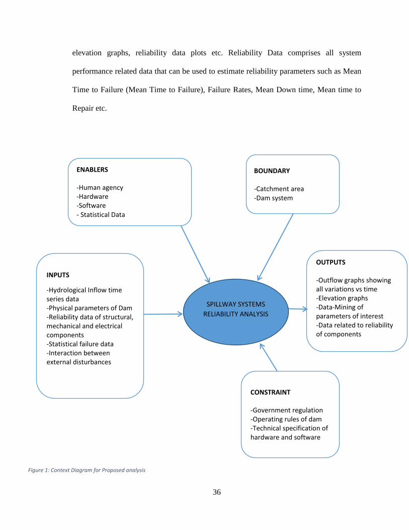
36
elevation graphs, reliability data plots etc. Reliability Data comprises all system
performance related data that can be used to estimate reliability parameters such as Mean
Time to Failure (Mean Time to Failure), Failure Rates, Mean Down time, Mean time to
Repair etc.
OUTPUTS
-Outflow graphs showing
all variations vs time
-Elevation graphs
-Data-Mining of
parameters of interest
-Data related to reliability
of components
CONSTRAINT
-Government regulation
-Operating rules of dam
-Technical specification of
hardware and software
BOUNDARY
-Catchment area
-Dam system
ENABLERS
-Human agency
-Hardware
-Software
- Statistical Data
SPILLWAY SYSTEMS
RELIABILITY ANALYSIS
INPUTS
-Hydrological Inflow time
series data
-Physical parameters of Dam
-Reliability data of structural,
mechanical and electrical
components
-Statistical failure data
-Interaction between
external disturbances
Figure 1: Context Diagram for Proposed analysis
37
2.4 REQUIREMENTS ANALYSIS
Requirements engineering (RE) lies at the heart of systems development, bridging the
gap between stakeholder goals and constraints, and their realization in systems that
inevitably combine technology and human processes, embedded in a changing
organizational context (Maté, 2005). RE is therefore multi-disciplinary in both its outlook
and its deployment of techniques for elicitation, specification, analysis, and management
of requirements.
Requirements engineering (RE) provides the methods, tools, and techniques to build the
roadmaps that designers and developers of complex software/people systems should
follow, as it is the discipline concerned with the real-world goals for, functions of, and
constraints on those systems (Zave, 1997).
2.4.1 SYSTEM LEVEL REQUIREMENTS FOR PROPOSED ANALYSIS FRAMEWORK The system-level requirements are general in nature, while requirements at low levels in
the hierarchy are very specific. The top-level system requirements defined in the system
requirements at this level are the main input for the requirements allocation and flow-
down phase. Three categories were defined at the systems level i.e., the Functional,
Performance and User Requirements. The functional requirements delineates the
computational and modeling aspects of what our proposed system needs to achieve. The
Performance requirements delineate what is required of the analysis system being
designed. Basically, this centers on the capabilities of the software platform needed to
implement the proposed analysis concept. The user requirements are generally at a higher
level than the technical requirements. They address the user-system interface
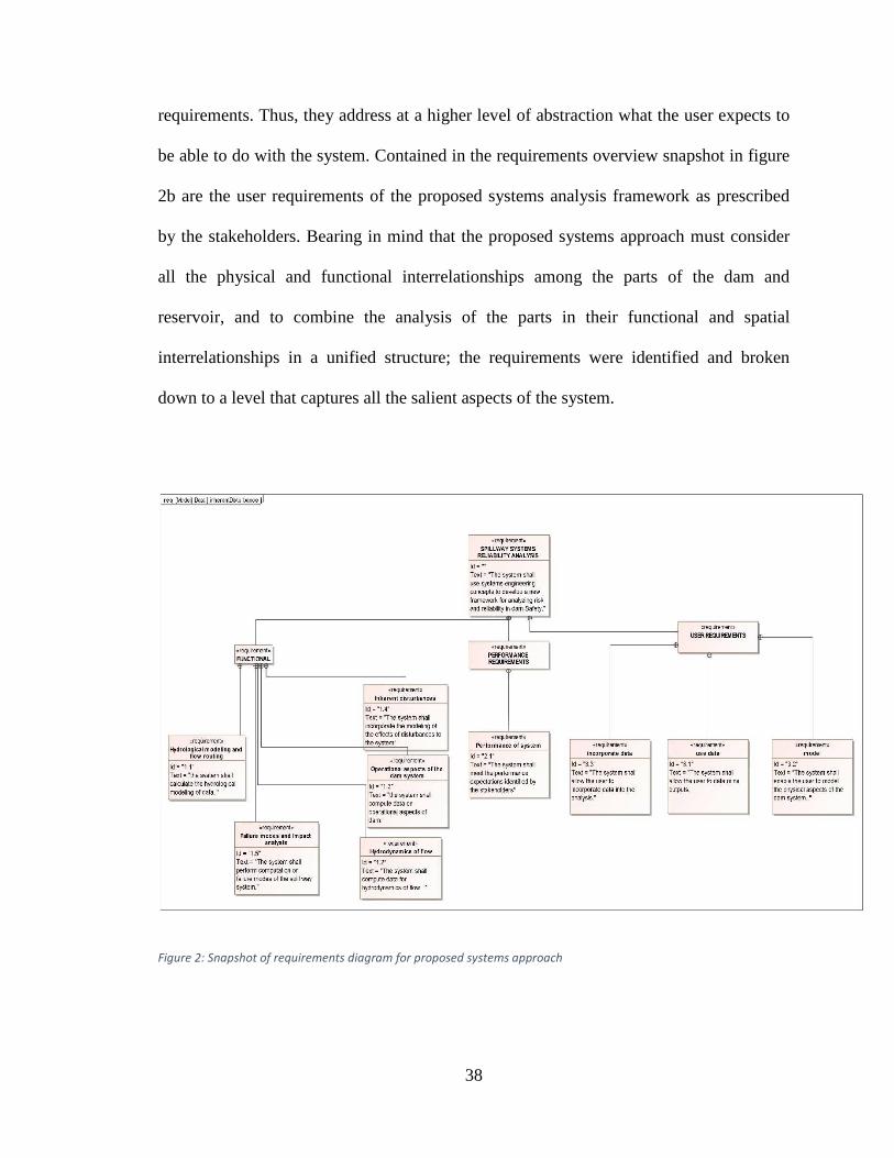
38
requirements. Thus, they address at a higher level of abstraction what the user expects to
be able to do with the system. Contained in the requirements overview snapshot in figure
2b are the user requirements of the proposed systems analysis framework as prescribed
by the stakeholders. Bearing in mind that the proposed systems approach must consider
all the physical and functional interrelationships among the parts of the dam and
reservoir, and to combine the analysis of the parts in their functional and spatial
interrelationships in a unified structure; the requirements were identified and broken
down to a level that captures all the salient aspects of the system.
Figure 2: Snapshot of requirements diagram for proposed systems approach
39
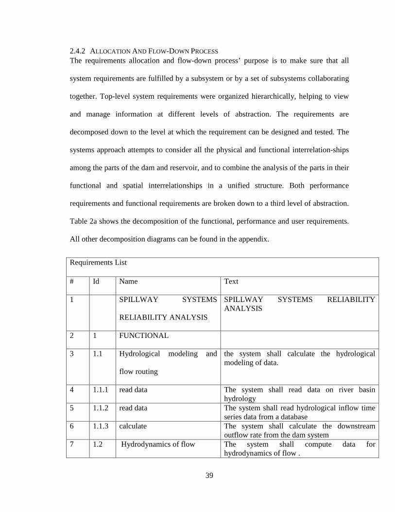
2.4.2 ALLOCATION AND FLOW-DOWN PROCESS The requirements allocation and flow-down process’ purpose is to make sure that all
system requirements are fulfilled by a subsystem or by a set of subsystems collaborating
together. Top-level system requirements were organized hierarchically, helping to view
and manage information at different levels of abstraction. The requirements are
decomposed down to the level at which the requirement can be designed and tested. The
systems approach attempts to consider all the physical and functional interrelation-ships
among the parts of the dam and reservoir, and to combine the analysis of the parts in their
functional and spatial interrelationships in a unified structure. Both performance
requirements and functional requirements are broken down to a third level of abstraction.
Table 2a shows the decomposition of the functional, performance and user requirements.
All other decomposition diagrams can be found in the appendix.
Requirements List
# Id Name Text
1 SPILLWAY SYSTEMS
RELIABILITY ANALYSIS
SPILLWAY SYSTEMS RELIABILITY ANALYSIS
2 1 FUNCTIONAL
3 1.1 Hydrological modeling and
flow routing
the system shall calculate the hydrological modeling of data.
4 1.1.1 read data The system shall read data on river basin hydrology
5 1.1.2 read data The system shall read hydrological inflow time series data from a database
6 1.1.3 calculate The system shall calculate the downstream outflow rate from the dam system
7 1.2 Hydrodynamics of flow The system shall compute data for hydrodynamics of flow .
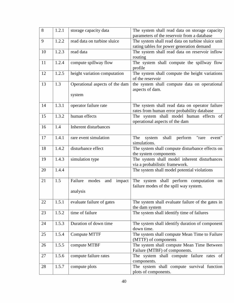
40
8 1.2.1 storage capacity data The system shall read data on storage capacity parameters of the reservoir from a database
9 1.2.2 read data on turbine sluice The system shall read data on turbine sluice unit rating tables for power generation demand
10 1.2.3 read data The system shall read data on reservoir inflow routing
11 1.2.4 compute spillway flow The system shall compute the spillway flow profile
12 1.2.5 height variation computation The system shall compute the height variations of the reservoir
13 1.3 Operational aspects of the dam
system
the system shall compute data on operational aspects of dam.
14 1.3.1 operator failure rate The system shall read data on operator failure rates from human error probability database
15 1.3.2 human effects The system shall model human effects of operational aspects of the dam
16 1.4 Inherent disturbances
17 1.4.1 rare event simulation The system shall perform "rare event" simulations.
18 1.4.2 disturbance effect The system shall compute disturbance effects on the system components
19 1.4.3 simulation type The system shall model inherent disturbances via a probabilistic framework.
20 1.4.4 The system shall model potential violations
21 1.5 Failure modes and impact
analysis
The system shall perform computation on failure modes of the spill way system.
22 1.5.1 evaluate failure of gates The system shall evaluate failure of the gates in the dam system
23 1.5.2 time of failure The system shall identify time of failures
24 1.5.3 Duration of down time The system shall identify duration of component down time.
25 1.5.4 Compute MTTF The system shall compute Mean Time to Failure (MTTF) of components
26 1.5.5 compute MTBF The system shall compute Mean Time Between Failure (MTBF) of components.
27 1.5.6 compute failure rates The system shall compute failure rates of components.
28 1.5.7 compute plots The system shall compute survival function plots of components.
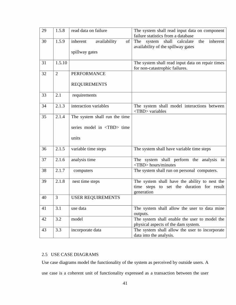
41
29 1.5.8 read data on failure The system shall read input data on component failure statistics from a database
30 1.5.9 inherent availability of
spillway gates
The system shall calculate the inherent availability of the spillway gates
31 1.5.10 The system shall read input data on repair times for non-catastrophic failures.
32 2 PERFORMANCE
REQUIREMENTS
33 2.1 requirements
34 2.1.3 interaction variables The system shall model interactions between <TBD> variables
35 2.1.4 The system shall run the time
series model in <TBD> time
units
36 2.1.5 variable time steps The system shall have variable time steps
37 2.1.6 analysis time The system shall perform the analysis in <TBD> hours/minutes
38 2.1.7 computers The system shall run on personal computers.
39 2.1.8 nest time steps The system shall have the ability to nest the time steps to set the duration for result generation
40 3 USER REQUIREMENTS
41 3.1 use data The system shall allow the user to data mine outputs.
42 3.2 model The system shall enable the user to model the physical aspects of the dam system.
43 3.3 incorporate data The system shall allow the user to incorporate data into the analysis.
2.5 USE CASE DIAGRAMS
Use case diagrams model the functionality of the system as perceived by outside users. A
use case is a coherent unit of functionality expressed as a transaction between the user
42
and the system (Maté, 2005). Thus use case diagrams allow us to elicit and describe
functional requirements. Use cases are alike in that they all describe to some degree the
series of actions and events the system and users perform during operation; however, they
are different in their focus and usage. The subsequent sections describe use cases for the
proposed approach to modeling risk and reliability in dam safety.
2.5.1 SYSTEMS LEVEL USE CASE The use case describes what the risk analyst does at a higher level of abstraction. As
illustrated in figure 2c, the user first builds the model, tunes it and then runs it. Once the
simulation run is complete, the Risk analyst can then choose to view the results and share
the outputs of the simulation study with the management. Management also provides the
data required to accurately characterize the system.
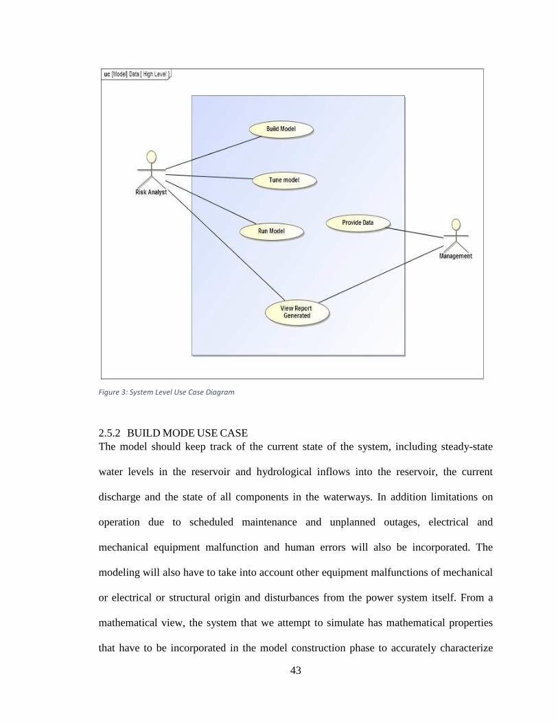
43
Figure 3: System Level Use Case Diagram
2.5.2 BUILD MODE USE CASE The model should keep track of the current state of the system, including steady-state
water levels in the reservoir and hydrological inflows into the reservoir, the current
discharge and the state of all components in the waterways. In addition limitations on
operation due to scheduled maintenance and unplanned outages, electrical and
mechanical equipment malfunction and human errors will also be incorporated. The
modeling will also have to take into account other equipment malfunctions of mechanical
or electrical or structural origin and disturbances from the power system itself. From a
mathematical view, the system that we attempt to simulate has mathematical properties
that have to be incorporated in the model construction phase to accurately characterize
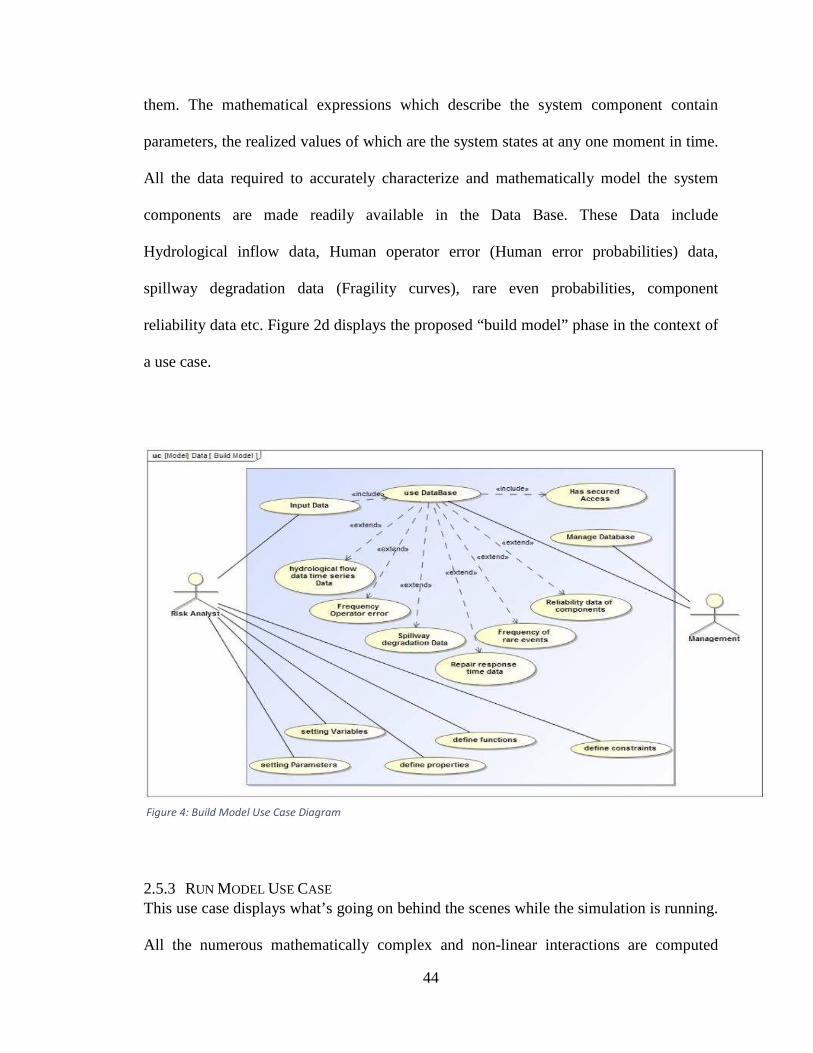
44
them. The mathematical expressions which describe the system component contain
parameters, the realized values of which are the system states at any one moment in time.
All the data required to accurately characterize and mathematically model the system
components are made readily available in the Data Base. These Data include
Hydrological inflow data, Human operator error (Human error probabilities) data,
spillway degradation data (Fragility curves), rare even probabilities, component
reliability data etc. Figure 2d displays the proposed “build model” phase in the context of
a use case.
Figure 4: Build Model Use Case Diagram
2.5.3 RUN MODEL USE CASE This use case displays what’s going on behind the scenes while the simulation is running.
All the numerous mathematically complex and non-linear interactions are computed
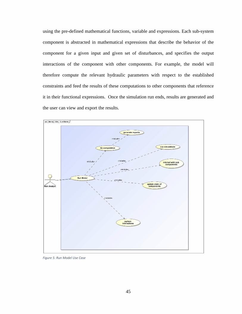
45
using the pre-defined mathematical functions, variable and expressions. Each sub-system
component is abstracted in mathematical expressions that describe the behavior of the
component for a given input and given set of disturbances, and specifies the output
interactions of the component with other components. For example, the model will
therefore compute the relevant hydraulic parameters with respect to the established
constraints and feed the results of these computations to other components that reference
it in their functional expressions. Once the simulation run ends, results are generated and
the user can view and export the results.
Figure 5: Run Model Use Case

46
2.6 ACTIVITY DIAGRAMS
Activity diagrams are a type of behavioral diagrams in the form of flowcharts of activities
within a portion of the system showing control flows between activities (Kossiakoff,
2011). They represent any type of flow inherent in a system, including processes,
operations, or control the sequence of activities and events is regulated via various
control nodes.
2.6.1 ANALYST ACTIVITY DIAGRAM
The activity diagram in figure 2f shows the complete set of activities happening in a
success scenario. The user inputs the data and builds the model depending on the values
defined. The user then tunes the model depending on the analysis required as mentioned
in the diagram. After selecting a value for each of the parameters the user runs the
analysis model which performs different computations and calculation depending on user
inputs. Once the system completes the intended analysis, required results are obtained.
Once the results are ready they can be viewed, deleted or stored for further analysis. For
details about different types of analysis and output, refer backup slide.
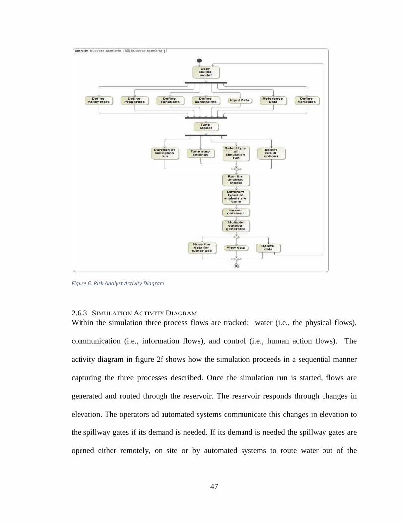
47
Figure 6: Risk Analyst Activity Diagram
2.6.3 SIMULATION ACTIVITY DIAGRAM Within the simulation three process flows are tracked: water (i.e., the physical flows),
communication (i.e., information flows), and control (i.e., human action flows). The
activity diagram in figure 2f shows how the simulation proceeds in a sequential manner
capturing the three processes described. Once the simulation run is started, flows are
generated and routed through the reservoir. The reservoir responds through changes in
elevation. The operators ad automated systems communicate this changes in elevation to
the spillway gates if its demand is needed. If its demand is needed the spillway gates are
opened either remotely, on site or by automated systems to route water out of the
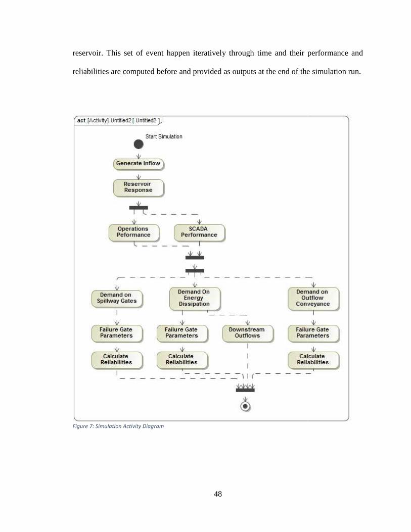
reservoir. This set of event happen iteratively through time and their performance and
reliabilities are computed befo
Figure 7: Simulation Activity Diagram
48
reservoir. This set of event happen iteratively through time and their performance and
reliabilities are computed before and provided as outputs at the end of the simulation run.
Simulation Activity Diagram
reservoir. This set of event happen iteratively through time and their performance and
re and provided as outputs at the end of the simulation run.

49
CHAPTER 3: LOWER MATTAGAMI RIVER BASIN CASE STUDY
3.1 BACKGROUND
The Lower Mattagami River Hydroelectric (LMR) Complex is comprised of four
hydroelectric generating plants, Smoky Falls Generation Station (GS), Little Long GS,
Harmon GS and Kipling GS. These facilities are located in the Moose River Basin about
90 km north of the Town of Kapuskasing, Ontario, Canada and are owned and operated
by Ontario Power Generation (OPG).Together, these four stations are known as the
Lower Mattagami River Hydroelectric Complex (LMR Complex). They are owned and
operated by Ontario Power Generation (OPG), the Proponent of the Project. Smoky Falls
GS is a base load station with four vertical Francis type units and a capacity of 52 MW.
Little Long GS, Harmon GS and Kipling GS each have two fixed-blade propeller type
units and operate as peaking stations with station capacities of 136 MW, 140 MW and
156 MW respectively. Smoky Falls GS was the first GS to come in service in 1931 while
Little Long GS, Harmon GS and Kipling GS all came in to service between 1963 and
1966.
3.1.1 LOCATION
The Mattagami River is located in the Moose River Basin (Shown in Figure 3) in
northeastern Ontario which encompasses a drainage area of 109,000 km2. It flows in a
northerly direction from its headwaters at Mesomikenda. Lake and is approximately 418
km long, covering a drainage basin area of 35,612 km2. The Mattagami River is
generally a shallow and slow-flowing river with a seasonal flow regime, characteristic of
rivers in the Moose River basin. The long-term average river flow for the Little Long GS

50
as recorded by OPG is approximately 412 m3/s, based on a period of record from 1926 to
2005. Since OPG’s hydroelectric stations along the LMR are in close succession,
intermediate drainage areas are small and the contribution from inflows between the
stations is not important for planning purposes.
The LMR Complex borders two physiographic regions: the Canadian Shield which
extends from the south to just north of Kipling GS and, beyond this, the Hudson Bay
Lowlands. Vegetation communities in the region are typical of the Northern Clay Belt
and Hudson Bay Lowlands sections of the Boreal Forest. The Mattagami River supports a
diverse fish community with a total of 28 known resident species.
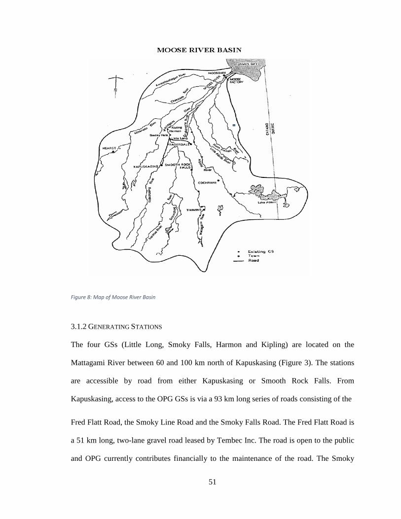
51
Figure 8: Map of Moose River Basin
3.1.2 GENERATING STATIONS
The four GSs (Little Long, Smoky Falls, Harmon and Kipling) are located on the
Mattagami River between 60 and 100 km north of Kapuskasing (Figure 3). The stations
are accessible by road from either Kapuskasing or Smooth Rock Falls. From
Kapuskasing, access to the OPG GSs is via a 93 km long series of roads consisting of the
Fred Flatt Road, the Smoky Line Road and the Smoky Falls Road. The Fred Flatt Road is
a 51 km long, two-lane gravel road leased by Tembec Inc. The road is open to the public
and OPG currently contributes financially to the maintenance of the road. The Smoky
52
Line Road is a 42 km long, single-lane gravel road owned by OPG. The Smoky Falls
Road is an 18 km long, two-lane gravel road, also owned by OPG.
Highway 643 (formerly Highway 807) links Smooth Rock Falls to Fraserdale via a 73 km
long two-lane paved road. The 46 km Little Long Road (Fraserdale Road) is a two-lane
gravel road that extends from Fraserdale to Little Long GS where it crosses the Little
Long dam and links up with the Smoky Falls Road. The Little Long road is owned and
maintained by OPG.
3.1.3 STATION CHARACTERISTICS
The area layout of the four GSs is shown in Figure 5. The Little Long, Harmon and
Kipling GSs were all constructed in the early 1960s and have similar operating heads,
hydraulic capacity and output. The GSs each have two units of the fixed-blade propeller
type and are operated in a peaking mode. Station capacities at Little Long GS, Harmon
GS and Kipling GS are 136, 140 and 156 MW, respectively. In contrast, Smoky Falls GS
is a 4-unit baseload station operating effectively 24 h/d with a station capacity of 52 MW.
Transmission of electrical energy from the four stations is provided by a 230 kV
transmission line from Kipling GS via Harmon GS to Little Long GS substation and from
there to the Pinard transformer station near Fraserdale. Generation from the existing
Smoky Falls GS is fed into a 115 kV transmission line that runs directly to the Tembec
paper mill in Kapuskasing. Relevant characteristics for each GS as well as the nearby
Adam Creek watershed are listed in Table 4a.
53
Figure 9: Characteristics of LMR Complex Stations
Figure 10: Characteristics of LMR Complex Stations
Notes: Turbine capacity at maximum continuous rating (MCR) at average head (as provided by OPG).
Average annual energy divided by capacity.
Includes recent turbine upgrades.
Combined spill capacity is 6087 m3/s. Maximum daily recorded flow at Little Long GS is 5070 m3/s.
Only two sluices are presently operational.
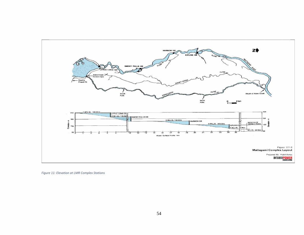
54
Figure 11: Elevation at LMR Complex Stations
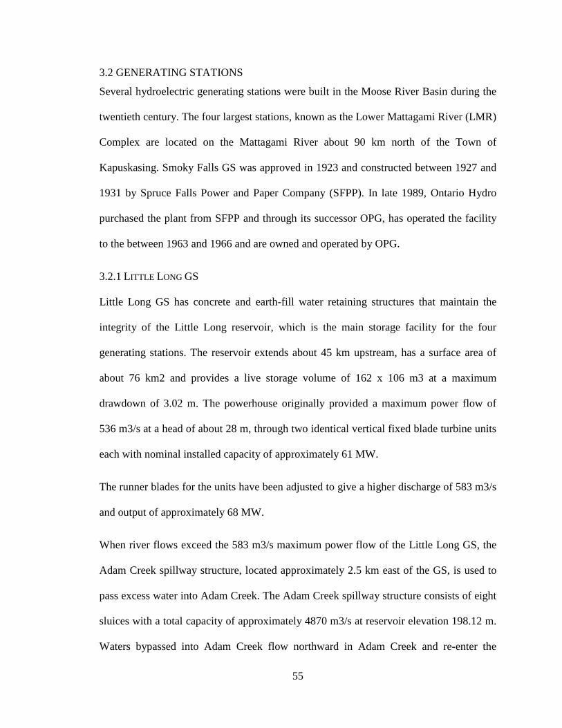
55
3.2 GENERATING STATIONS
Several hydroelectric generating stations were built in the Moose River Basin during the
twentieth century. The four largest stations, known as the Lower Mattagami River (LMR)
Complex are located on the Mattagami River about 90 km north of the Town of
Kapuskasing. Smoky Falls GS was approved in 1923 and constructed between 1927 and
1931 by Spruce Falls Power and Paper Company (SFPP). In late 1989, Ontario Hydro
purchased the plant from SFPP and through its successor OPG, has operated the facility
to the between 1963 and 1966 and are owned and operated by OPG.
3.2.1 LITTLE LONG GS
Little Long GS has concrete and earth-fill water retaining structures that maintain the
integrity of the Little Long reservoir, which is the main storage facility for the four
generating stations. The reservoir extends about 45 km upstream, has a surface area of
about 76 km2 and provides a live storage volume of 162 x 106 m3 at a maximum
drawdown of 3.02 m. The powerhouse originally provided a maximum power flow of
536 m3/s at a head of about 28 m, through two identical vertical fixed blade turbine units
each with nominal installed capacity of approximately 61 MW.
The runner blades for the units have been adjusted to give a higher discharge of 583 m3/s
and output of approximately 68 MW.
When river flows exceed the 583 m3/s maximum power flow of the Little Long GS, the
Adam Creek spillway structure, located approximately 2.5 km east of the GS, is used to
pass excess water into Adam Creek. The Adam Creek spillway structure consists of eight
sluices with a total capacity of approximately 4870 m3/s at reservoir elevation 198.12 m.
Waters bypassed into Adam Creek flow northward in Adam Creek and re-enter the
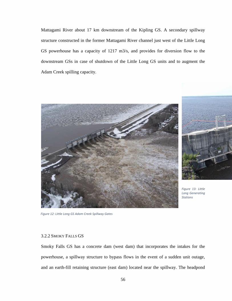
56
Mattagami River about 17 km downstream of the Kipling GS. A secondary spillway
structure constructed in the former Mattagami River channel just west of the Little Long
GS powerhouse has a capacity of 1217 m3/s, and provides for diversion flow to the
downstream GSs in case of shutdown of the Little Long GS units and to augment the
Adam Creek spilling capacity.
Figure 13: Little
Long Generating
Stations
3.2.2 SMOKY FALLS GS
Smoky Falls GS has a concrete dam (west dam) that incorporates the intakes for the
powerhouse, a spillway structure to bypass flows in the event of a sudden unit outage,
and an earth-fill retaining structure (east dam) located near the spillway. The headpond
Figure 12: Little Long GS Adam Creek Spillway Gates

57
extends upstream for about 7 km, has a surface area of about 5.3 km2 and a live storage
volume of 6.7 x 10⁶ m3 at a maximum drawdown of 3.05 m. The powerhouse contains
four vertical Francis type turbine units, with the capacity to generate 52 MW at a rated
flow of approximately 190 m3/s and an operating head of 34.5 m. The existing spillway
structure consists of 10 gated sluices, each being 8.4 m wide by 9.2 m high, plus an
approximately 230 m long overflow crest. The spillway structure was originally designed
(prior to the construction of the Adam Creek Diversion) to convey what was then the full
design flood flow on the Mattagami River. With the construction of the Adam Creek
Diversion, the spillway only needs to maintain a discharge capacity of 1217 m3/s. Two of
the 10 gates are operational and the overflow section is permanently sealed with timber
stop logs.

58
Figure 15: Smokey Falls Generating Stations
3.2.3 HARMON GS
Figure 14: Smokey Falls Spillway Gates
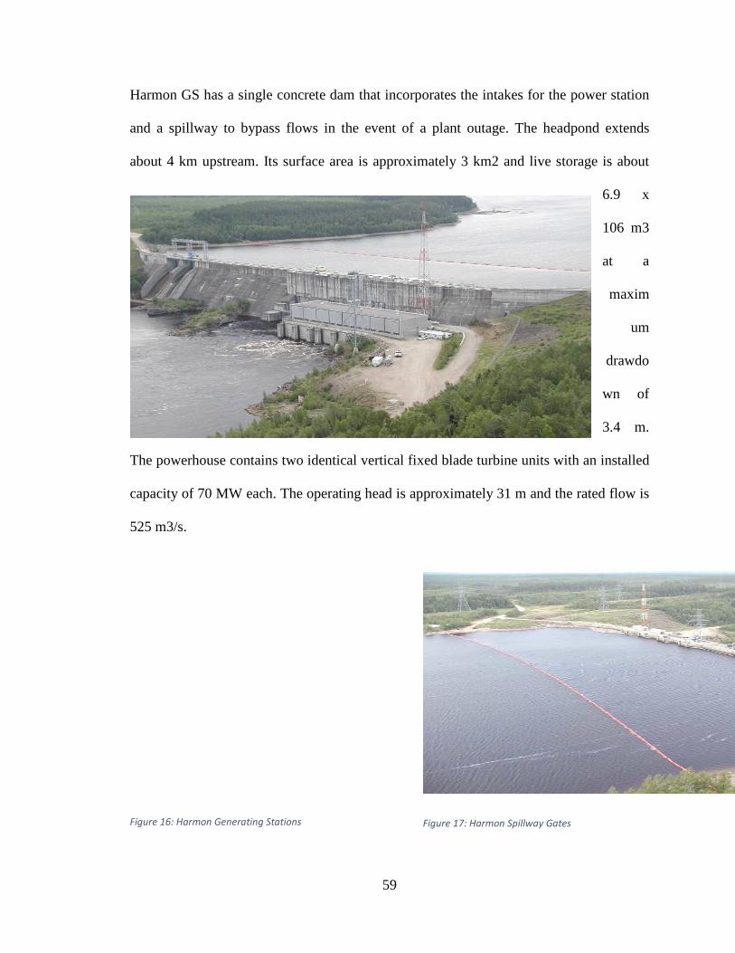
59
Harmon GS has a single concrete dam that incorporates the intakes for the power station
and a spillway to bypass flows in the event of a plant outage. The headpond extends
about 4 km upstream. Its surface area is approximately 3 km2 and live storage is about
6.9 x
106 m3
at a
maxim
um
drawdo
wn of
3.4 m.
The powerhouse contains two identical vertical fixed blade turbine units with an installed
capacity of 70 MW each. The operating head is approximately 31 m and the rated flow is
525 m3/s.
Figure 17: Harmon Spillway Gates
Figure 16: Harmon Generating Stations
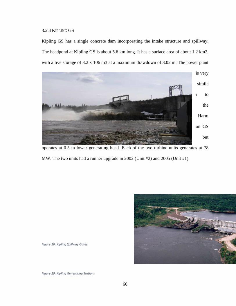
60
3.2.4 KIPLING GS
Kipling GS has a single concrete dam incorporating the intake structure and spillway.
The headpond at Kipling GS is about 5.6 km long. It has a surface area of about 1.2 km2,
with a live storage of 3.2 x 10⁶ m3 at a maximum drawdown of 3.02 m. The power plant
is very
simila
r to
the
Harm
on GS
but
operates at 0.5 m lower generating head. Each of the two turbine units generates at 78
MW. The two units had a runner upgrade in 2002 (Unit #2) and 2005 (Unit #1).
Figure 19: Kipling Generating Stations
Figure 18: Kipling Spillway Gates

61
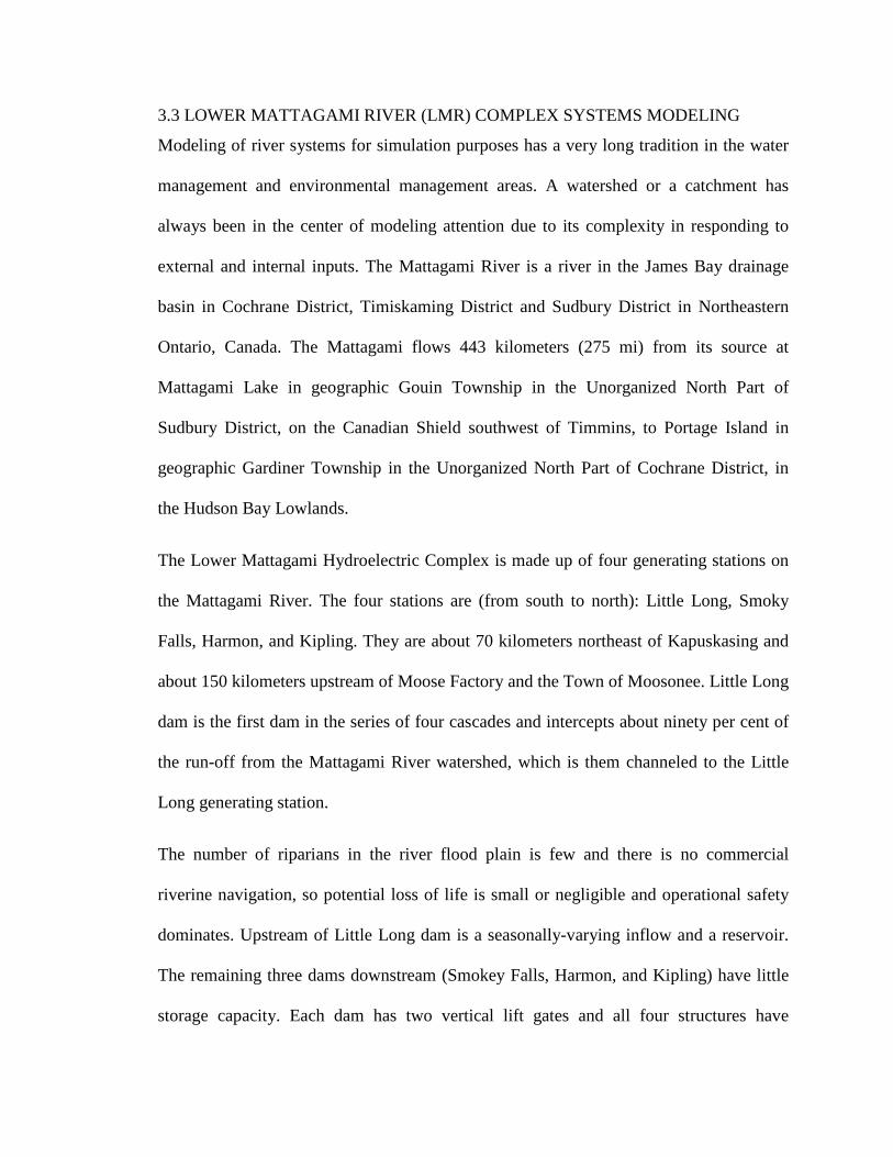
3.3 LOWER MATTAGAMI RIVER (LMR) COMPLEX SYSTEMS MODELING
Modeling of river systems for simulation purposes has a very long tradition in the water
management and environmental management areas. A watershed or a catchment has
always been in the center of modeling attention due to its complexity in responding to
external and internal inputs. The Mattagami River is a river in the James Bay drainage
basin in Cochrane District, Timiskaming District and Sudbury District in Northeastern
Ontario, Canada. The Mattagami flows 443 kilometers (275 mi) from its source at
Mattagami Lake in geographic Gouin Township in the Unorganized North Part of
Sudbury District, on the Canadian Shield southwest of Timmins, to Portage Island in
geographic Gardiner Township in the Unorganized North Part of Cochrane District, in
the Hudson Bay Lowlands.
The Lower Mattagami Hydroelectric Complex is made up of four generating stations on
the Mattagami River. The four stations are (from south to north): Little Long, Smoky
Falls, Harmon, and Kipling. They are about 70 kilometers northeast of Kapuskasing and
about 150 kilometers upstream of Moose Factory and the Town of Moosonee. Little Long
dam is the first dam in the series of four cascades and intercepts about ninety per cent of
the run-off from the Mattagami River watershed, which is them channeled to the Little
Long generating station.
The number of riparians in the river flood plain is few and there is no commercial
riverine navigation, so potential loss of life is small or negligible and operational safety
dominates. Upstream of Little Long dam is a seasonally-varying inflow and a reservoir.
The remaining three dams downstream (Smokey Falls, Harmon, and Kipling) have little
storage capacity. Each dam has two vertical lift gates and all four structures have
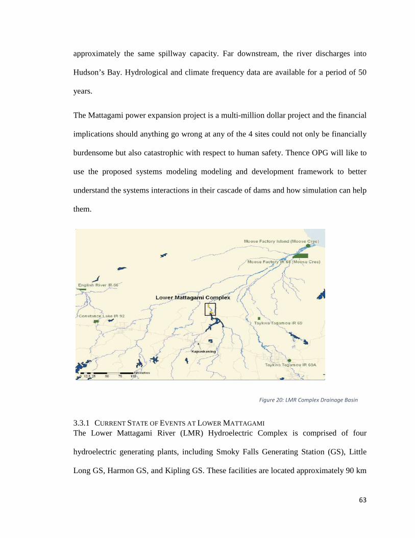
approximately the same spillway capa
Hudson’s Bay. Hydrological and climate frequency data a
years.
The Mattagami power expansion project is a multi
implications should anything go wrong at any of the 4 sites could not only be financially
burdensome but also catastrophic with respect to human safety. Thence OPG wi
use the proposed systems modeling model
understand the systems interactions in their cascade of dams and how simulation can help
them.
3.3.1 CURRENT STATE OF
The Lower Mattagami River (LMR) Hydroe
hydroelectric generating plants, including
Long GS, Harmon GS, and Kipling G
approximately the same spillway capacity. Far downstream, the river
Hudson’s Bay. Hydrological and climate frequency data are available for a period of 50
The Mattagami power expansion project is a multi-million dollar project and the financial
implications should anything go wrong at any of the 4 sites could not only be financially
burdensome but also catastrophic with respect to human safety. Thence OPG wi
proposed systems modeling modeling and development framework to better
understand the systems interactions in their cascade of dams and how simulation can help
TATE OF EVENTS AT LOWER MATTAGAMI The Lower Mattagami River (LMR) Hydroelectric Complex is comprised of
hydroelectric generating plants, including Smoky Falls Generating Station
Long GS, Harmon GS, and Kipling GS. These facilities are located approximately 90 km
Figure 20: LMR Complex Drainage Basin
63
city. Far downstream, the river discharges into
re available for a period of 50
million dollar project and the financial
implications should anything go wrong at any of the 4 sites could not only be financially
burdensome but also catastrophic with respect to human safety. Thence OPG will like to
ing and development framework to better
understand the systems interactions in their cascade of dams and how simulation can help
lectric Complex is comprised of four
Smoky Falls Generating Station (GS), Little
approximately 90 km
Figure 20: LMR Complex Drainage Basin
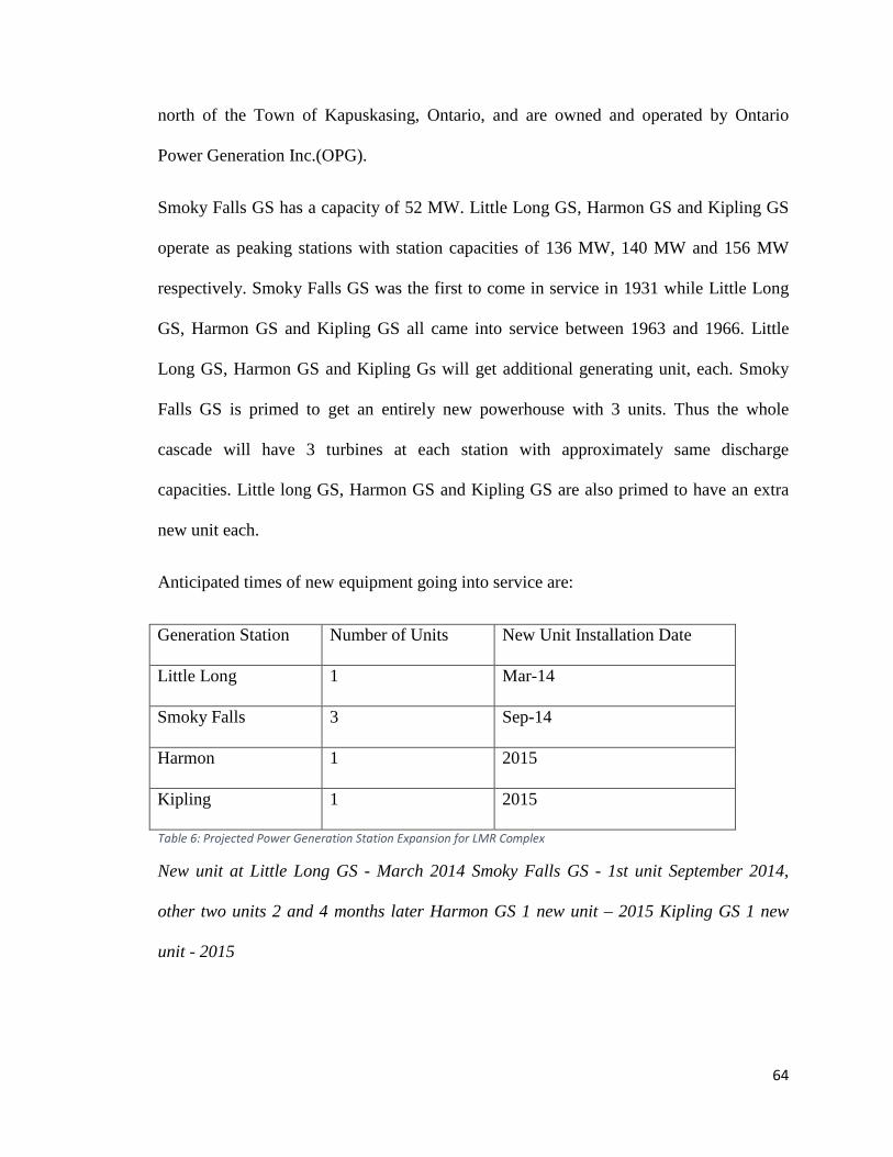
64
north of the Town of Kapuskasing, Ontario, and are owned and operated by Ontario
Power Generation Inc.(OPG).
Smoky Falls GS has a capacity of 52 MW. Little Long GS, Harmon GS and Kipling GS
operate as peaking stations with station capacities of 136 MW, 140 MW and 156 MW
respectively. Smoky Falls GS was the first to come in service in 1931 while Little Long
GS, Harmon GS and Kipling GS all came into service between 1963 and 1966. Little
Long GS, Harmon GS and Kipling Gs will get additional generating unit, each. Smoky
Falls GS is primed to get an entirely new powerhouse with 3 units. Thus the whole
cascade will have 3 turbines at each station with approximately same discharge
capacities. Little long GS, Harmon GS and Kipling GS are also primed to have an extra
new unit each.
Anticipated times of new equipment going into service are:
Generation Station Number of Units New Unit Installation Date
Little Long 1 Mar-14
Smoky Falls 3 Sep-14
Harmon 1 2015
Kipling 1 2015
Table 6: Projected Power Generation Station Expansion for LMR Complex
New unit at Little Long GS - March 2014 Smoky Falls GS - 1st unit September 2014,
other two units 2 and 4 months later Harmon GS 1 new unit – 2015 Kipling GS 1 new
unit - 2015
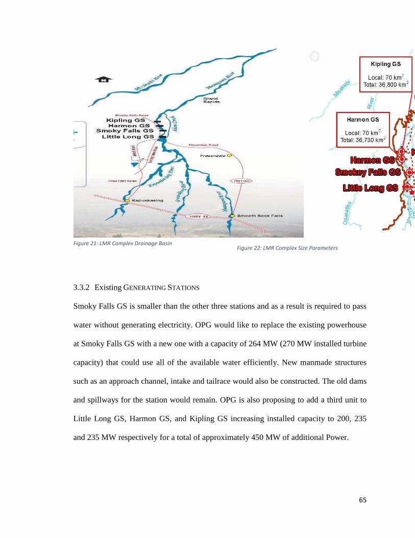
65
Figure 22: LMR Complex Size Parameters
3.3.2 Existing GENERATING STATIONS
Smoky Falls GS is smaller than the other three stations and as a result is required to pass
water without generating electricity. OPG would like to replace the existing powerhouse
at Smoky Falls GS with a new one with a capacity of 264 MW (270 MW installed turbine
capacity) that could use all of the available water efficiently. New manmade structures
such as an approach channel, intake and tailrace would also be constructed. The old dams
and spillways for the station would remain. OPG is also proposing to add a third unit to
Little Long GS, Harmon GS, and Kipling GS increasing installed capacity to 200, 235
and 235 MW respectively for a total of approximately 450 MW of additional Power.
Figure 21: LMR Complex Drainage Basin
66
3.4.1 CORE OBJECTIVES OF THE LOWER MATTAGAMI RIVER CASE STUDY
Applying the proposed systems modeling concept to OPG’s Lower Mattagami System to
better understand the systems interactions in their cascade of four dams; this involves
dams at Smoky Falls, Little Long, Harmon and Kipling. All four dams are primed for
upgrades to their Power Generation capacities within the next 2 years. The core
objectives of the project are listed below:
• Applying the systems modeling framework developed in the SSRP to OPG’s
Lower Mattagami System to better understand the systems interactions in their
cascade of four dams; this involves dams at Smoky Falls, Little Long, Harmon
and Kipling.
• Formulating and constructing a model to accurately characterize the physics of
hydrodynamics including the dynamics of transport, Storage and power
generation. Holistically integrating into the model, river basin hydrology, the
routing of inflows through the reservoir system, operating rules and human factors
of operating the spillway, and the dam component fragilities (structural,
mechanical and electrical).
• Generate stochastic time series by using the historic inflow time series to forecast
inflows for several thousand years and multiple replications to identify unforeseen
chain of events that could lead to dam system failure.
• Reviewing the current operating rules to determine whether further optimization
techniques can be adopted to improve the power generation capabilities of the
system.
67
• Modeling the inherent disturbances (Lightening, Seismic, Floating Ice, Grid
disturbances and Debris) via a probabilistic framework.
• Incorporating Human reliability analysis (HRA) into the model by using expert
judgment and available data to estimate human error probabilities on spillway
gate operations with regards to failure.
3.4.2 FEATURES
The modeling activities allow different conceptual approaches to be analyzed and
compared. The level of modeling in this report is kept at the more general ‘logical’ level
and is a means of exploring how BC Hydro’s interests can be met. It would be possible to
develop a more detailed ‘physical’ model referring to specific equipment selections but
such detail is not justified until the logical modeling has allowed the main system
configurations to be explored.
3.5 VIEWPOINTS
The main viewpoints of interest for the LMR complex systems modeling are:
a. Safety (a mandatory consideration for a safety assessment);
b. Reliability (includes surveillance, the assurance of reliability by routine inspection and
testing);
c. Operability (the organization and decision making structure to operate safely).
68
3.6 MAJOR RISKS IDENTIFIED RISKS
The main risks to the safe operation of the dam can be summarized as:
a. The loss of remote control through communications or other failure;
b. Incorrect management decisions, for any reason, that fail to establish the appropriate
spill profile for the prevailing conditions;
c. The loss of power supplies or other supporting or auxiliary services;
d. The loss of access to the dam in emergency;
e. Unpredictable and excessive weather;
f. Common cause disruption such as fire;
g. Failure of control or instrumentation;
h. A lack of qualified personnel to provide an emergency response;
i. Failure of the gates or supporting structures.
3.7 SYSTEMS AND STUDY BOUNDARIES
The full boundary of the Mattagami River System is presented in the appendix. A
snapshot of the system schematic is provided in figure 19. This shows the Lower
Mattagami cascade of four dams from Little Long to Kipling with an overview of their
Power output capacities, discharge capacities of spillway gates and the power generating
turbines and operating ranges. Figure 21 shows the system boundary of this case study,
water head elevations from one dam to the other and the major bypass Adam Creek.
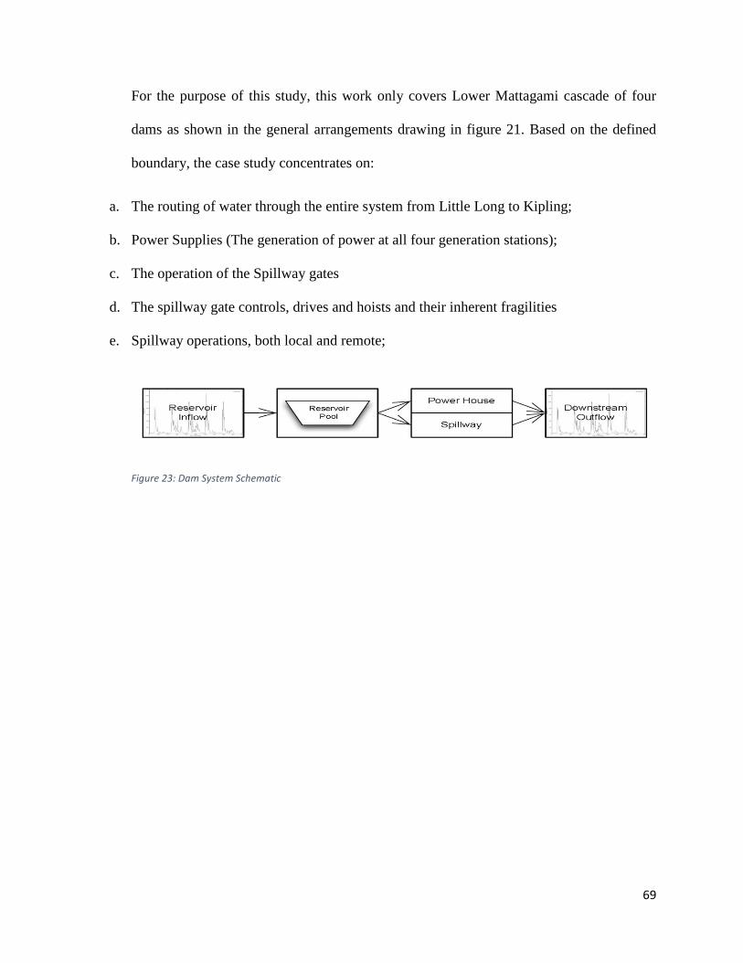
69
For the purpose of this study, this work only covers Lower Mattagami cascade of four
dams as shown in the general arrangements drawing in figure 21. Based on the defined
boundary, the case study concentrates on:
a. The routing of water through the entire system from Little Long to Kipling;
b. Power Supplies (The generation of power at all four generation stations);
c. The operation of the Spillway gates
d. The spillway gate controls, drives and hoists and their inherent fragilities
e. Spillway operations, both local and remote;
Figure 23: Dam System Schematic
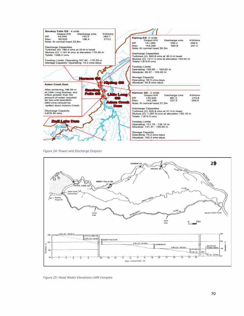
70
Figure 24: Power and Discharge Outputs
Figure 25: Head Water Elevations LMR Complex
71
3.8 GOLDSIM™ MODELING FRAMEWORK
3.8.1 BACKGROUND TO GOLDSIM™ AND THE RELIABILITY MODULE
For many engineered systems, it is necessary to predict measures such as the system's
reliability (the probability that a component or system will perform its required function
over a specified time period) and availability (the probability that a component or system
is performing its required function at any given time).
By combining the flexibility of a general-purpose and highly-graphical probabilistic
simulation framework that can directly model the movement of material through a
system, with specialized features to support reliability analysis and optimization,
GoldSim™ allows you to create quantitative and transparent reliability and throughput
models to allow you to ask "what if" questions regarding various designs and make
defensible risk management decisions. GoldSim™ is most valuable when analyzing
complex systems with many subsystems.
GoldSim™ can be thought of as a high-level programming language, where the program
is the model. The analyst joins together objects called “elements” using “links” to create
the model of the system. Elements, which may represent either physical or logical
components of the system, will often have a stochastic component, and the links carry
information between the elements.
Realistic analysis of such systems is best facilitated by a “total system” model that
represents the interactions, interdependencies and feedback between the various system
components (including humans). Without such a model, it may not be possible to identify
potential bottlenecks, failure mechanisms, fatal flaws or system incompatibilities.
72
The modeler creates a representation of the system in its initial state, imbuing the
elements with the appropriate properties, behaviors, and relationships. Then, when the
simulation is started, the software takes over and evaluates the entire history of the
system, saving selected results for subsequent analysis.
3.8.2 THE RELIABILITY MODULE
The reliability module is an add-on to the standard GoldSim™ simulation framework,
consisting of two new element types: the Function element and the Action element. The
Function element is used to model components that perform their function over a period
of time (e.g., a battery or an environmental control system), while Action elements are
used to model components that perform their duties only when triggered by a specific
condition or conditions (e.g., a relay, or an actuator). The primary output of a reliability
element is its operating state at any given time during the simulation: whether it is
operating or not.
3.9 WHY GOLDSIM™?
GoldSim™ is a Monte Carlo simulation software solution for dynamically modeling
complex systems in business, engineering and science. GoldSim™ supports decision and
risk analysis by simulating future performance while quantitatively representing the
uncertainty and risks inherent in all complex systems.
The GoldSim™ software is highly graphical and extensible, able to quantitatively
represent the uncertainty inherent in complex systems, and allows users to create
compelling models that are easy to communicate and explain to diverse audiences. Users
build a model in an intuitive manner by literally drawing a picture (an influence diagram)
of their system. In a sense, GoldSim™ is like a “visual spreadsheet” that allows users to
73
graphically create and manipulate data and equations. It moves beyond spreadsheets,
however, by making it much easier for users to evaluate how systems evolve over time
and predict their future behavior.
Water resources and hydrological modeling projects typically involve simulating systems
made up of many component parts that are interrelated. In most situations, the
hydrological system is driven by stochastic variables (i.e., runoff, precipitation,
evaporation, demand) and involves uncertain processes, parameters, and events. The
challenge when evaluating water supply and resource systems is to find an approach that
can incorporate all the knowledge available into a quantitative framework that can be
used to simulate and predict the outcome of alternative approaches and policies.
By combining the flexibility of a general-purpose and highly-graphical probabilistic
simulation framework with specialized modules to support mass transport modeling,
reliability analysis, and optimization, GoldSim™ simulation software is optimized to
create realistic models of water supply, water resource, hydraulic and hydrological
systems in order to carry out risk analyses, evaluate potential environmental impacts,
support strategic planning, and make better resource management decisions.

4. HYDROLOGIC MODELING AND FLOW ROUTING
There is no single and unique definition of a river system and the definitions may change
depending on the purpose of the study of the system being undertaken. According to
Dunne (2009), “River systems are complex systems through which irregular fluxes of
water and mobile terrestrial materials derived from the lithosphere, atmosphere,
biosphere, and techno-sphere are focused.”
What is of interest in applications of systems approach to regulated river networks are the
models of river systems. A model is only a physical or mathematical representation of the
system itself and of the interrelations and interactions between the system elements. As
such the models are only simplified and idealized abstractions of reality and usually do
not describe the entire modelled reality. But it should be noted that this should not
necessarily disqualify the model since the purpose of the modeling activity can be often
characterized as achieving only prescribed accuracy within the predefined time and
budget constraints (Baecher, 2014)
A definition of a river system model in this paper can be developed along the following
general principles:
• A system can be defined as a collection of interrelated elements purposely working
toward achieving some common objective;
• Most of the natural systems or systems that include natural systems can be characterized
as dynamic systems because the collection of elements constantly interacts over time;

75
• The elements of the system can be subdivided into the following three groups:
components, attributes and relationships. These three distinctive groups can be
characterized as:
• Components or subsystems are the operating parts of a system and consist of input,
process and output. Components can take the form of natural or technological artefacts.
Each component may assume a variety of values defining the system state;
• Attributes are the properties or discernible manifestations of the system, its
components and the relationships between them;
• Relationships are the links between components and attributes. The properties and
behavior of each component of the system influence the properties and behavior of the
system as a whole. At the same time, each component depends up-on the properties and
behavior of at least one other component in the system. Because of this interdependence,
the components cannot be divided into independent subsets; the system is more than the
sum of its parts. Also, if a component is removed from a system or if its characteristics
change, the other artefacts in the system will alter characteristics accordingly, and the
relationships among them may also change (Carlsson, 2002).
• River networks whether in natural state or regulated (with human-made structures) can
thus be understood as systems;
• Behavior of the river system can be characterized by quantities that vary in time (water
levels, flows, velocities at different places within the system, etc.);
• The components of a river system are:
76
- Reservoirs providing storage behind the dams;
- Natural and artificial channels;
- Diversion and control structures (dams);
- Confluence points;
- Local sub-basins (sub-watersheds).
It is important to understand at this point that such a definition of the model of a river
system is not universal and may be inadequate for purposes that differ from the purpose
of this paper. The Mattagami River System-on which this paper is predicated- includes
dams, and thus the system is a regulated river system and the purpose of the regulation is
to satisfy the needs of various water uses. These uses include hydropower generation,
navigation support, flood control etc.
4.1 HISTORIC TIME SERIES DATA
50 year historic time series data on reservoir inflows from the lower Mattagami to Little
Long will be used to generate Stochastic Reservoir Inflows through time series
forecasting. The complexity of the time series forecasting is not at the highest level since
the emphasis on this thesis is on promulgating the systems concept and not necessarily
achieving accurate time series models. The method adopted for forecasting the local
inflows coming into little long reservoir are listed as follows.
77
• In this particular case study, as already explained the emphasis is not on the accuracy of
time series forecasting techniques and hence the historic data (Inflow time series) was
used to populate a forward looking Time Series.
• Having established that, the next step was to apply that historic data to the simulation
(which looks forward in time). In order to do this, therefore, there was the need to time
shift the data so that the historic data is applied in an appropriate and consistent manner.
• How this works is, a random starting point is chosen from the historic series to
incorporate some level of uncertainty in forwarding the historic series. This option
randomly samples a starting point in the data set for each realization. This is useful since
we have 50 years of inflow data, and want GoldSim™ to randomly sample a different
historic start year for each realization.
• The Data periodicity is set as “annual”, which means GoldSim™ ensures that the random
starting point for each realization is sampled such that all starting points are a multiple of
1 (average) year apart. In particular, random starting points for successive realizations
are always multiples of 365.25 days apart (rounded to the nearest day).
• This option shifts the time series data forward (or backward) by a multiple of a year such
that the simulation begins by using data from the specified Data year to start in. For
instance, if the actual data set started on 31 July1989 and ended on 31 December 2011,
the Simulation Start Date was 1 January 2013, and the Data year to start in was entered as
1990, GoldSim™ would treat the data set such that the data point corresponding to 1
January 1990 would be used for 1 January 2013 (and, assuming daily data was entered,
the data point for 2 January 1990 would be used for 2 January 2013, etc.).
78
• To account for uncertainty and randomness while still directly using the historic data, the
use of random starting point option with “annual periodicity” suits the purpose of this
study.
• The “Enable Time Shifting of Time Series Data” option was chosen in the advanced
settings in the GoldSim™ Time Series Element and GoldSim™ automatically wraps
around to the start of the data set if the end of the data set is reached during a simulation.
The manner in which this is done depends on the periodicity of the data.
• By using a random starting point with annual periodicity and aligning data years with
simulation dates, when the end of the data set is reached, the data set is effectively
replicated and shifted forward by N years, where N is the number of whole years in the
data set. For example, if there were 3.5 years of data in the data set, the last data point
was on December 31, and the simulation extended beyond 3.5 years, the data set would
be shifted forward by 3 years, so that the first occurrence of January 1 in the data set
would follow the last point in the data set.
4.2 THE MODELED SYSTEM SCHEMATIC
Figure 22 shows snapshot of the general model interface showcasing the salient aspects
of the physical system being modeled. It shows representation of the system in its initial
state, imbuing the elements with the appropriate properties, behaviors, and relationships.
Then, when the simulation is started, the software takes over and evaluates the entire
history of the system, saving selected results for subsequent analysis.
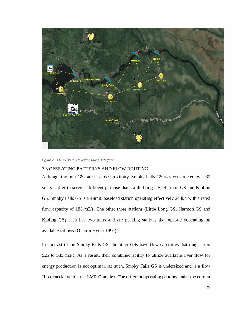
79
Figure 26: LMR System Simulation Model Interface
3.3 OPERATING PATTERNS AND FLOW ROUTING
Although the four GSs are in close proximity, Smoky Falls GS was constructed over 30
years earlier to serve a different purpose than Little Long GS, Harmon GS and Kipling
GS. Smoky Falls GS is a 4-unit, baseload station operating effectively 24 h/d with a rated
flow capacity of 188 m3/s. The other three stations (Little Long GS, Harmon GS and
Kipling GS) each has two units and are peaking stations that operate depending on
available inflows (Ontario Hydro 1990).
In contrast to the Smoky Falls GS, the other GSs have flow capacities that range from
525 to 585 m3/s. As a result, their combined ability to utilize available river flow for
energy production is not optimal. As such, Smoky Falls GS is undersized and is a flow
“bottleneck” within the LMR Complex. The different operating patterns under the current
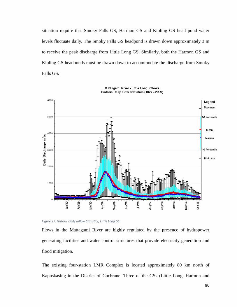
80
situation require that Smoky Falls GS, Harmon GS and Kipling GS head pond water
levels fluctuate daily. The Smoky Falls GS headpond is drawn down approximately 3 m
to receive the peak discharge from Little Long GS. Similarly, both the Harmon GS and
Kipling GS headponds must be drawn down to accommodate the discharge from Smoky
Falls GS.
Figure 27: Historic Daily Inflow Statistics, Little Long GS
Flows in the Mattagami River are highly regulated by the presence of hydropower
generating facilities and water control structures that provide electricity generation and
flood mitigation.
The existing four-station LMR Complex is located approximately 80 km north of
Kapuskasing in the District of Cochrane. Three of the GSs (Little Long, Harmon and

81
Kipling) each have two units and are peaking stations with flow capacities ranging from
525 to 585 m3/s while the fourth station, Smoky Falls GS, is a 4-unit, baseload station
operating 24 h/d with a rated flow capacity of 188 m3/s. In comparison, the existing
Smoky Falls GS has less flow capacity for energy production.
During the spring freshet, flows in the Mattagami River typically exceed the flow
capacities of the GSs and therefore must be diverted through the Adam Creek Diversion.
Adam Creek then discharges this overflow into the Mattagami River at a point
approximately 17 km downstream of the Kipling GS (section 5.2.1.3 below). Figure 5.2-1
presents historic daily inflows to Little Long GS headpond. When flows exceed 583
m3/s, excess water that cannot be utilized by the Mattagami River GSs is diverted to
Adam Creek. As shown in Figure 5.2-1, the average peak daily flows during the spring
freshet are above 1,500 m3/s and can be quite variable. Appendix F provides the flow
duration curves for each month and for a total year.
4.4 FLOW ROUTING AT LITTLE LONG
The current state of events requires Little Long to generate electricity at full capacity
within its operating range. This means the turbines will be operated at maximum best
efficiency flow until the lower operating limit at of the Little Long Reservoir is reached;
at which point the turbine flow becomes equal to the inflow into the reservoir if inflows
fall below the flow required for best efficiency flow. On the other hand, if inflows are
greater than the requirements for best efficiency flow, the excess is used to fill up the
Reservoir until its peak operating limit. In this case the excess Inflow is spilled through
the Adam creek bypass. There are 8 gates that open into the Adam creek and two that
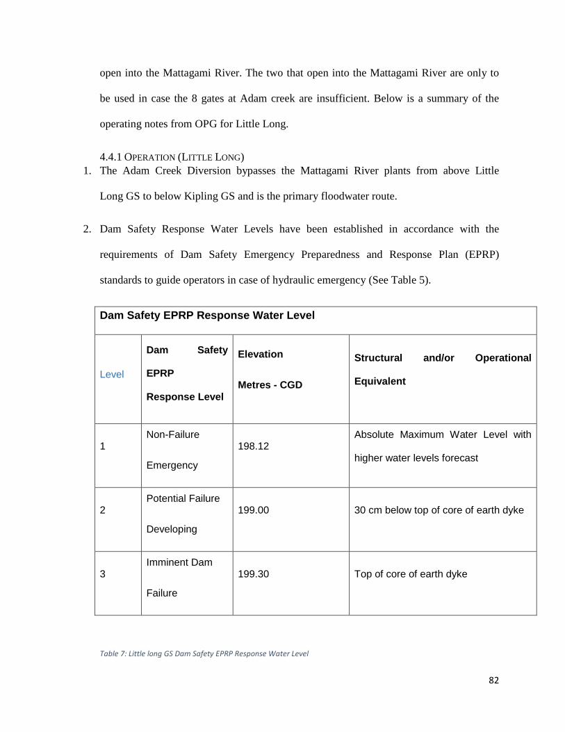
82
open into the Mattagami River. The two that open into the Mattagami River are only to
be used in case the 8 gates at Adam creek are insufficient. Below is a summary of the
operating notes from OPG for Little Long.
4.4.1 OPERATION (LITTLE LONG) 1. The Adam Creek Diversion bypasses the Mattagami River plants from above Little
Long GS to below Kipling GS and is the primary floodwater route.
2. Dam Safety Response Water Levels have been established in accordance with the
requirements of Dam Safety Emergency Preparedness and Response Plan (EPRP)
standards to guide operators in case of hydraulic emergency (See Table 5).
Dam Safety EPRP Response Water Level
Level
Dam Safety
EPRP
Response Level
Elevation
Metres - CGD
Structural and/or Operational
Equivalent
1 Non-Failure
Emergency
198.12 Absolute Maximum Water Level with
higher water levels forecast
2 Potential Failure
Developing
199.00 30 cm below top of core of earth dyke
3 Imminent Dam
Failure
199.30 Top of core of earth dyke
Table 7: Little long GS Dam Safety EPRP Response Water Level

83
3. At the start of freshet, the Little Long forebay should be filled to an elevation not
exceeding 198.00 metres. After achieving that elevation, any inflow greater than the
amount of water required for two-unit operation (583 m3/s) should be spilled down
Adams Creek. The reason for this maximum level of 198.00 metres is to allow for safe
operation of the station in the event of a contingency that results in the loss of units and
operating control (e.g. a lightning strike). Such a contingency would make it impossible
to remotely control sluice gate operation of Adams Creek. This 12-centimeter of storage
will allow for the four hour time lag required to dispatch operator agents to the station to
deal with the contingency. The maximum forebay level of 198.00 meters is during the
freshet period only. There is no requirement to spill through the main dam. This practice
should be avoided to improve operating efficiency at Smoky Falls during freshet.
Another reason for avoiding this practice is to eliminate the stranding of sturgeon in the
spillway pools and the subsequent rescue operation. The forebay should be filled
gradually to 198.12 metres in the last seven days of freshet.
3. Sluicegates 5, 6, 9, and 10 are controlled locally by the operator agents at the gates.
Two to four hours may be required to reach the site. There is a concern of further
undermining of the sluiceway apron at Adams Creek sluicegates 8 and 9. An engineering
assessment, which included a diving inspection, carried out in September 1996 confirmed
that no restrictions are required on sluicegates 3 to 10 at this time. The area is to be re-
inspected subsequent to each major spill in which sluicegates 8 and 9 are utilized. As a
minimum, the area of the sluiceway apron is to be inspected every three years. The last
inspection in July 2001 reported no further erosion of the bedrock below the sluice apron
since 1996.
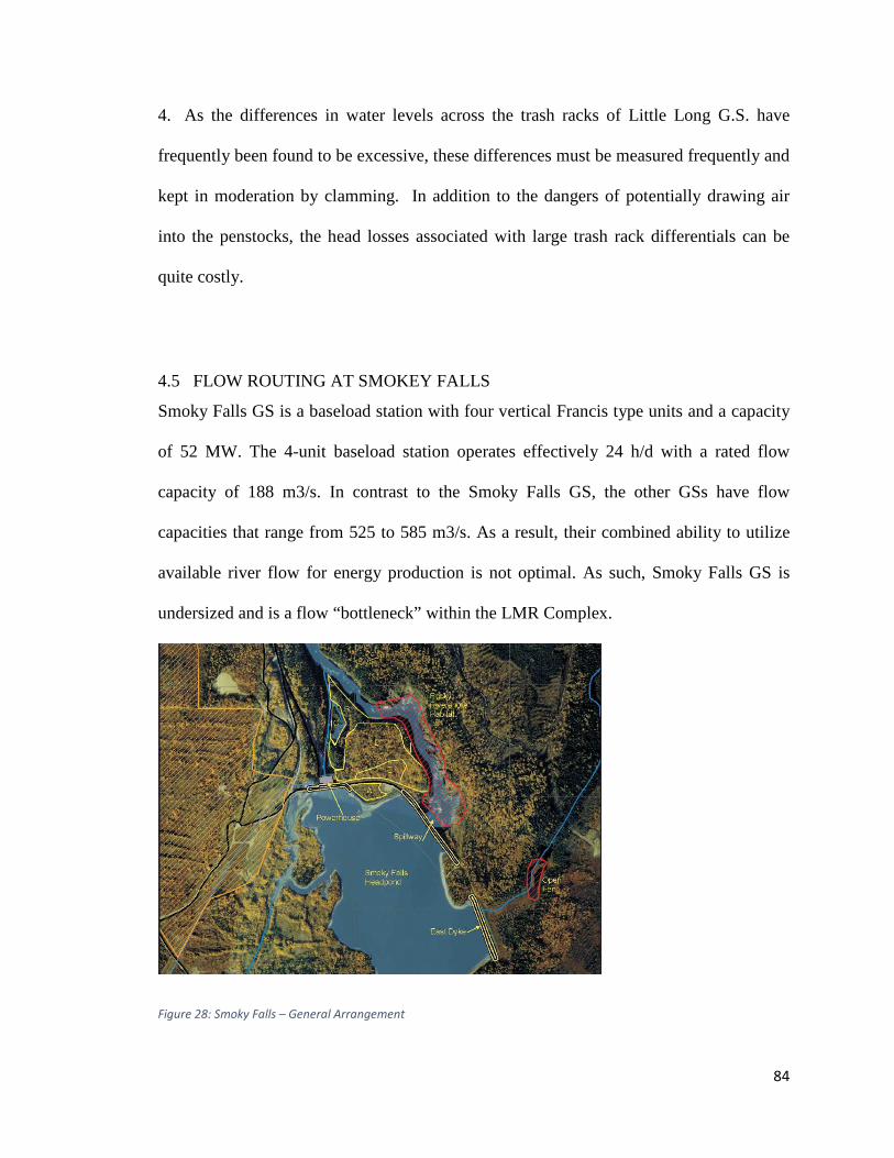
84
4. As the differences in water levels across the trash racks of Little Long G.S. have
frequently been found to be excessive, these differences must be measured frequently and
kept in moderation by clamming. In addition to the dangers of potentially drawing air
into the penstocks, the head losses associated with large trash rack differentials can be
quite costly.
4.5 FLOW ROUTING AT SMOKEY FALLS
Smoky Falls GS is a baseload station with four vertical Francis type units and a capacity
of 52 MW. The 4-unit baseload station operates effectively 24 h/d with a rated flow
capacity of 188 m3/s. In contrast to the Smoky Falls GS, the other GSs have flow
capacities that range from 525 to 585 m3/s. As a result, their combined ability to utilize
available river flow for energy production is not optimal. As such, Smoky Falls GS is
undersized and is a flow “bottleneck” within the LMR Complex.
Figure 28: Smoky Falls – General Arrangement

85
4.5.1 OPERATION (SMOKEY) 1. Several operating restrictions are required when maintenance work is being completed at
the draft tube level under the runner at Smoky Falls GS. During this time, the tailrace is
limited to a maximum elevation of 135.09 m and the combined (plant plus sluicegate)
discharge is limited to 350 m3/s. The maximum Harmon GS headwater during this time
period is limited to 133.40 m.
2. The elevation of the top of the sluicegates is 170.30 m. A 15-centimeter board has been
added to the top of the sluicegates in order to achieve the forebay maximum elevation of
170.45 m. The maximum forebay elevation may have to be reduced in the fall to prevent
water splashing over the top, thus building up ice and possibly making the sluicegates
unavailable for remote operation.
3. The #2 sluicegate is equipped with DC backup to operate the gate upon the loss of station
service.
4. During high inflow periods (freshet) when both Little Long units are generating at
maximum gate continually, lower the Smoky Falls forebay to 168.00 meters. The
resulting head increase at Little Long will create a net gain of 3 or more MW including
the lowered output at Smoky Falls.
3.6 HARMON OPERATIONS
1. Adam Creek Diversion bypasses the main river from above Little Long GS to below
Kipling GS and is the primary and major floodwater route. Inflows exceeding station
capacity are passed through the sluice gates.
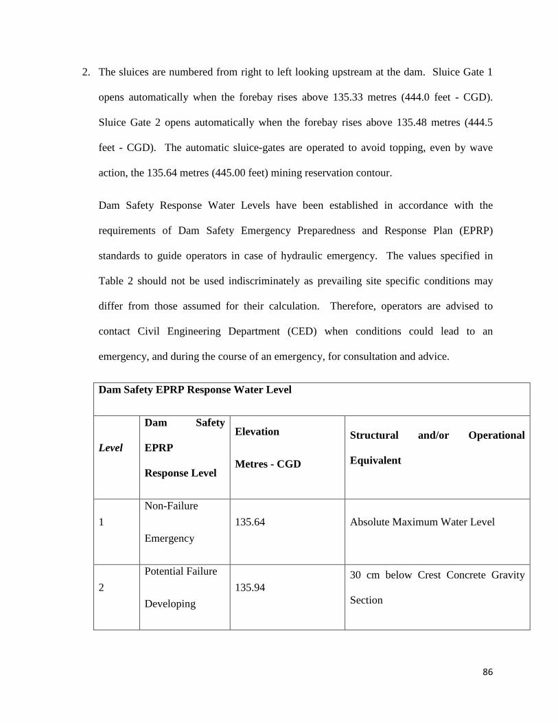
86
2. The sluices are numbered from right to left looking upstream at the dam. Sluice Gate 1
opens automatically when the forebay rises above 135.33 metres (444.0 feet - CGD).
Sluice Gate 2 opens automatically when the forebay rises above 135.48 metres (444.5
feet - CGD). The automatic sluice-gates are operated to avoid topping, even by wave
action, the 135.64 metres (445.00 feet) mining reservation contour.
Dam Safety Response Water Levels have been established in accordance with the
requirements of Dam Safety Emergency Preparedness and Response Plan (EPRP)
standards to guide operators in case of hydraulic emergency. The values specified in
Table 2 should not be used indiscriminately as prevailing site specific conditions may
differ from those assumed for their calculation. Therefore, operators are advised to
contact Civil Engineering Department (CED) when conditions could lead to an
emergency, and during the course of an emergency, for consultation and advice.
Dam Safety EPRP Response Water Level
Level
Dam Safety
EPRP
Response Level
Elevation
Metres - CGD
Structural and/or Operational
Equivalent
1
Non-Failure
Emergency
135.64 Absolute Maximum Water Level
2
Potential Failure
Developing
135.94 30 cm below Crest Concrete Gravity
Section
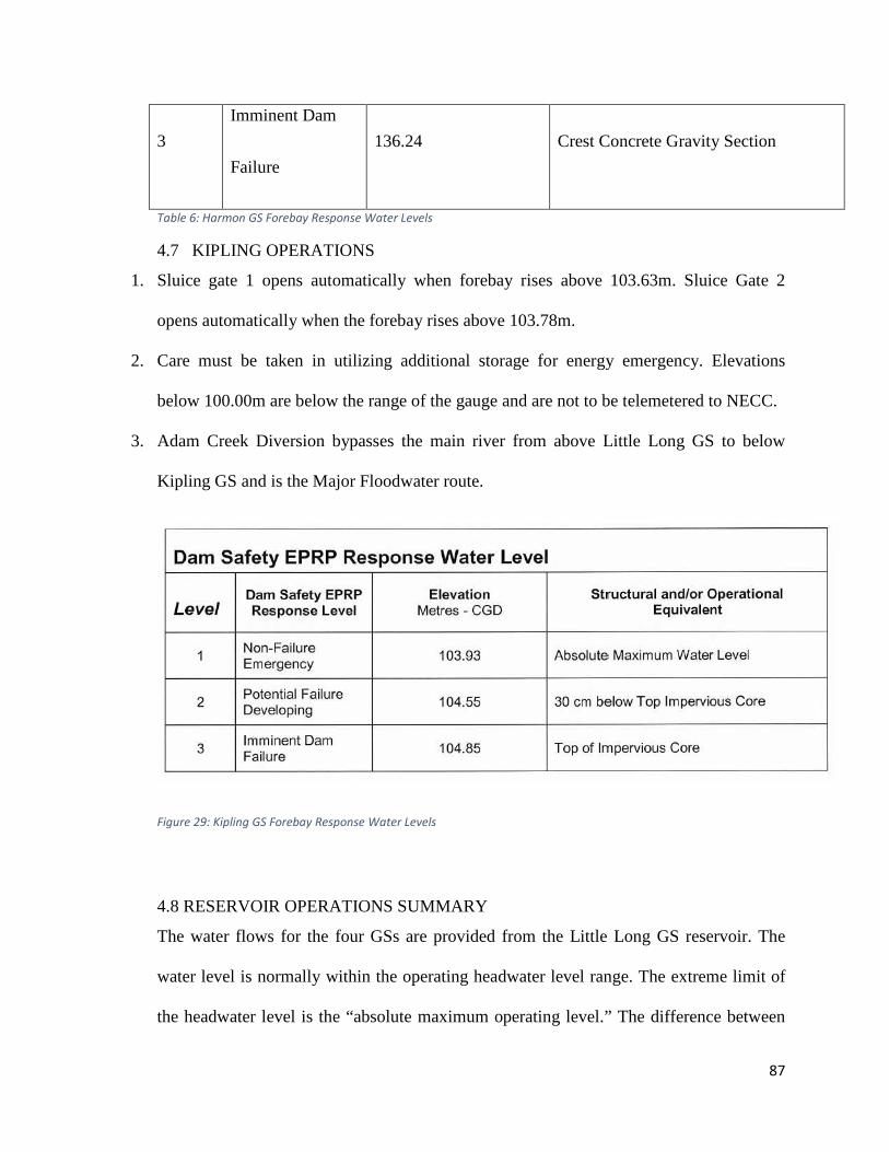
87
3
Imminent Dam
Failure
136.24 Crest Concrete Gravity Section
Table 6: Harmon GS Forebay Response Water Levels
4.7 KIPLING OPERATIONS
1. Sluice gate 1 opens automatically when forebay rises above 103.63m. Sluice Gate 2
opens automatically when the forebay rises above 103.78m.
2. Care must be taken in utilizing additional storage for energy emergency. Elevations
below 100.00m are below the range of the gauge and are not to be telemetered to NECC.
3. Adam Creek Diversion bypasses the main river from above Little Long GS to below
Kipling GS and is the Major Floodwater route.
Figure 29: Kipling GS Forebay Response Water Levels
4.8 RESERVOIR OPERATIONS SUMMARY
The water flows for the four GSs are provided from the Little Long GS reservoir. The
water level is normally within the operating headwater level range. The extreme limit of
the headwater level is the “absolute maximum operating level.” The difference between
88
the absolute maximum and maximum operating levels is referred to as the “flood
allowance”, which is only used to hold water in extreme conditions to reduce downstream
flooding. The storage between the absolute minimum and minimum operating levels is
only used if a system energy emergency occurs. Under normal operating conditions with
equivalent discharges at each station, the full operating range in the Smoky Falls GS,
Harmon GS and Kipling GS head ponds would rarely be utilized and headpond levels
will be significantly more stable during operation.
4.8.1 SUMMARY SPILLWAY OPERATIONS Under normal operating conditions, the outflow from the Little Long GS reservoir will
pass through all the GSs. During any outage of a GS, the spillway at the station
experiencing the outage will be operated to pass the desired flow to the other GSs.
During high river flow conditions (e.g., spring runoff) when the Little Long GS reservoir
is near its maximum limit, the spillway at Adam Creek will be operated in conjunction
with Little Long GS to pass the full Mattagami River flow.
4.9 POWER GENERATION
The Lower Mattagami Hydroelectric Complex Project has provided peaking and baseload
power to the Ontario grid for industrial, commercial and residential consumers since
1963. The Little Long, Harmon and Kipling GSs were all constructed in the early 1960s
and have similar operating heads, hydraulic capacity and output. The GSs each have two
units of the fixed-blade propeller type and are operated in a peaking mode. Station
capacities at Little Long GS, Harmon GS and Kipling GS are 136, 140 and 156 MW,
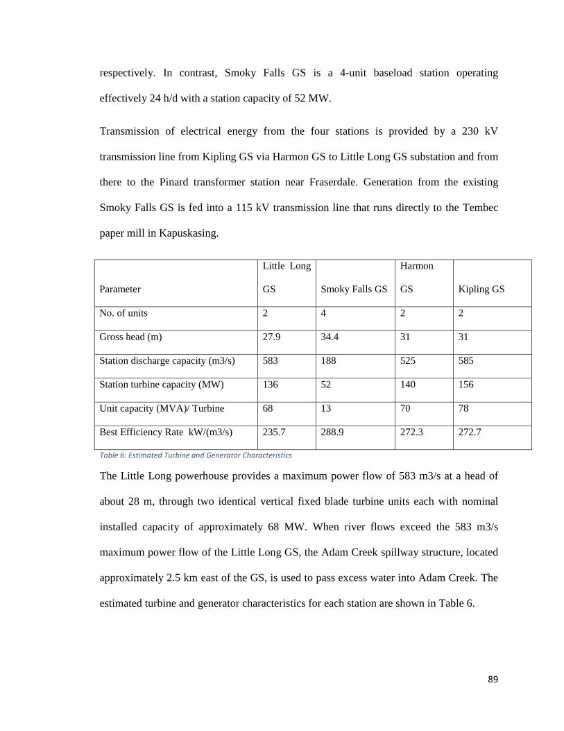
89
respectively. In contrast, Smoky Falls GS is a 4-unit baseload station operating
effectively 24 h/d with a station capacity of 52 MW.
Transmission of electrical energy from the four stations is provided by a 230 kV
transmission line from Kipling GS via Harmon GS to Little Long GS substation and from
there to the Pinard transformer station near Fraserdale. Generation from the existing
Smoky Falls GS is fed into a 115 kV transmission line that runs directly to the Tembec
paper mill in Kapuskasing.
Parameter
Little Long
GS Smoky Falls GS
Harmon
GS Kipling GS
No. of units 2 4 2 2
Gross head (m) 27.9 34.4 31 31
Station discharge capacity (m3/s) 583 188 525 585
Station turbine capacity (MW) 136 52 140 156
Unit capacity (MVA)/ Turbine 68 13 70 78
Best Efficiency Rate kW/(m3/s) 235.7 288.9 272.3 272.7
Table 6: Estimated Turbine and Generator Characteristics
The Little Long powerhouse provides a maximum power flow of 583 m3/s at a head of
about 28 m, through two identical vertical fixed blade turbine units each with nominal
installed capacity of approximately 68 MW. When river flows exceed the 583 m3/s
maximum power flow of the Little Long GS, the Adam Creek spillway structure, located
approximately 2.5 km east of the GS, is used to pass excess water into Adam Creek. The
estimated turbine and generator characteristics for each station are shown in Table 6.
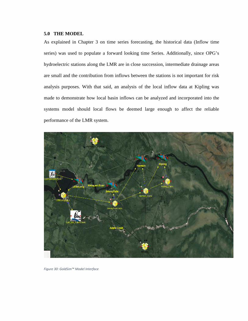
5.0 THE MODEL
As explained in Chapter 3 on time series forecasting, the historical data (Inflow time
series) was used to populate a forward looking time Series. Additionally, since OPG’s
hydroelectric stations along the LMR are in close succession, intermediate drainage areas
are small and the contribution from inflows between the stations is not important for risk
analysis purposes. With that said, an analysis of the local inflow data at Kipling was
made to demonstrate how local basin inflows can be analyzed and incorporated into the
systems model should local flows be deemed large enough to affect the reliable
performance of the LMR system.
Figure 30: GoldSim™ Model Interface
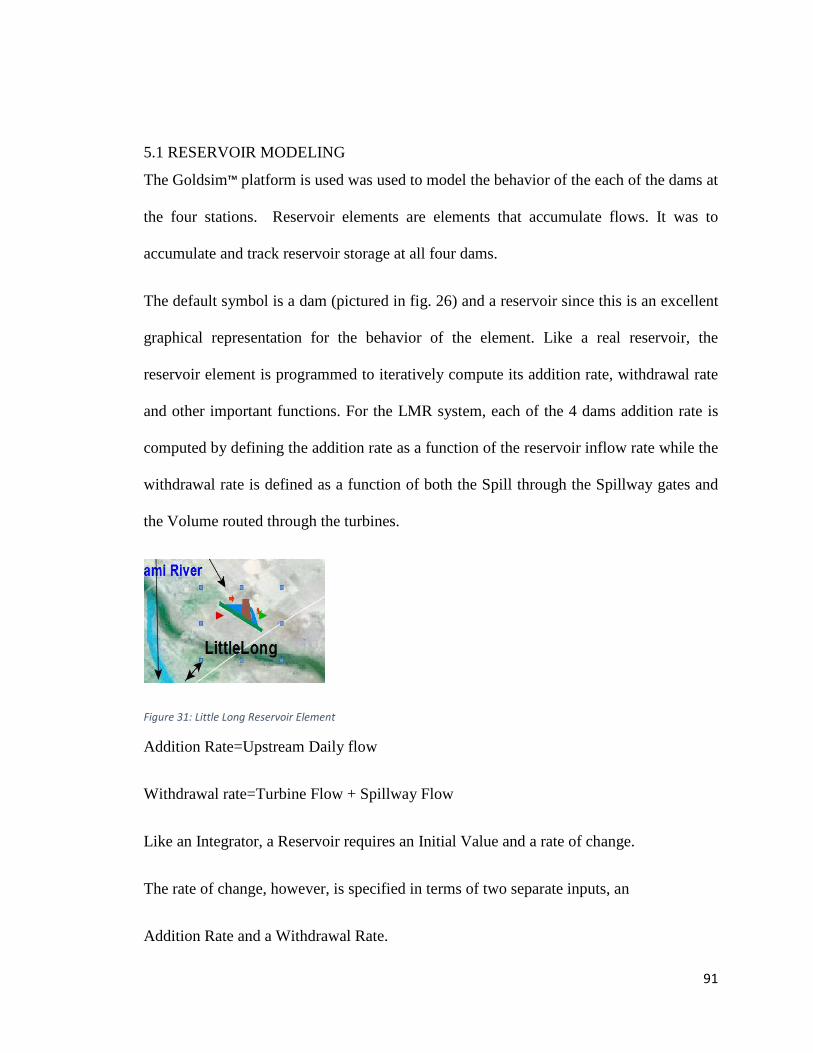
91
5.1 RESERVOIR MODELING
The Goldsim™ platform is used was used to model the behavior of the each of the dams at
the four stations. Reservoir elements are elements that accumulate flows. It was to
accumulate and track reservoir storage at all four dams.
The default symbol is a dam (pictured in fig. 26) and a reservoir since this is an excellent
graphical representation for the behavior of the element. Like a real reservoir, the
reservoir element is programmed to iteratively compute its addition rate, withdrawal rate
and other important functions. For the LMR system, each of the 4 dams addition rate is
computed by defining the addition rate as a function of the reservoir inflow rate while the
withdrawal rate is defined as a function of both the Spill through the Spillway gates and
the Volume routed through the turbines.
Figure 31: Little Long Reservoir Element
Addition Rate=Upstream Daily flow
Withdrawal rate=Turbine Flow + Spillway Flow
Like an Integrator, a Reservoir requires an Initial Value and a rate of change.
The rate of change, however, is specified in terms of two separate inputs, an
Addition Rate and a Withdrawal Rate.
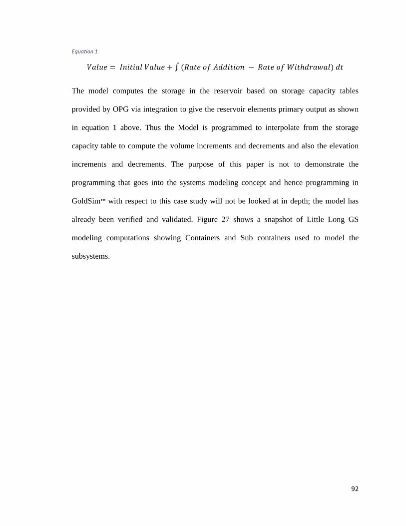
92
Equation 1
����� � ������ ����� � � ���� �� ������� � ��� �� ������ ��! �
The model computes the storage in the reservoir based on storage capacity tables
provided by OPG via integration to give the reservoir elements primary output as shown
in equation 1 above. Thus the Model is programmed to interpolate from the storage
capacity table to compute the volume increments and decrements and also the elevation
increments and decrements. The purpose of this paper is not to demonstrate the
programming that goes into the systems modeling concept and hence programming in
GoldSim™ with respect to this case study will not be looked at in depth; the model has
already been verified and validated. Figure 27 shows a snapshot of Little Long GS
modeling computations showing Containers and Sub containers used to model the
subsystems.
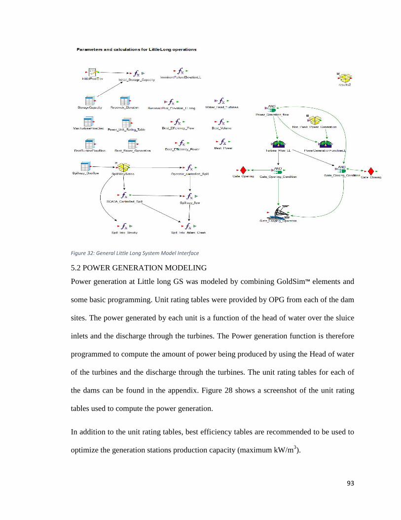
93
Figure 32: General Little Long System Model Interface
5.2 POWER GENERATION MODELING
Power generation at Little long GS was modeled by combining GoldSim™ elements and
some basic programming. Unit rating tables were provided by OPG from each of the dam
sites. The power generated by each unit is a function of the head of water over the sluice
inlets and the discharge through the turbines. The Power generation function is therefore
programmed to compute the amount of power being produced by using the Head of water
of the turbines and the discharge through the turbines. The unit rating tables for each of
the dams can be found in the appendix. Figure 28 shows a screenshot of the unit rating
tables used to compute the power generation.
In addition to the unit rating tables, best efficiency tables are recommended to be used to
optimize the generation stations production capacity (maximum kW/m3).
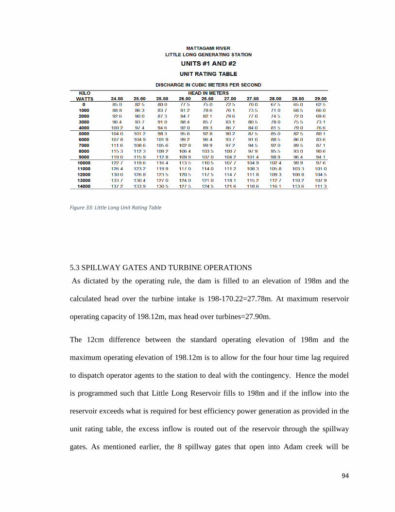
94
Figure 33: Little Long Unit Rating Table
5.3 SPILLWAY GATES AND TURBINE OPERATIONS
As dictated by the operating rule, the dam is filled to an elevation of 198m and the
calculated head over the turbine intake is 198-170.22=27.78m. At maximum reservoir
operating capacity of 198.12m, max head over turbines=27.90m.
The 12cm difference between the standard operating elevation of 198m and the
maximum operating elevation of 198.12m is to allow for the four hour time lag required
to dispatch operator agents to the station to deal with the contingency. Hence the model
is programmed such that Little Long Reservoir fills to 198m and if the inflow into the
reservoir exceeds what is required for best efficiency power generation as provided in the
unit rating table, the excess inflow is routed out of the reservoir through the spillway
gates. As mentioned earlier, the 8 spillway gates that open into Adam creek will be

95
operated first and if they are insufficient, the additional 2 gates that open into the
Mattagami River will be used to supplement the spill. Currently, there is no requirement
to spill through the main dam. This practice is avoided to improve operating efficiency at
Smoky Falls during freshet.
Consequently, if the inflow into the reservoir is below what is required for best efficiency
flow, and the reservoir elevation is at the minimum operating elevation, then same head is
maintained while inflow water (or equivalent volume) is routed through turbine intake
sluices. On the other hand if the inflow into the reservoir is less than the minimum for
best efficiency flow but the reservoir elevation is above the minimum operating
elevation, then the reservoir elevation is gradually lowered while generating the
minimum best efficiency power until the minimum operating threshold is crossed.
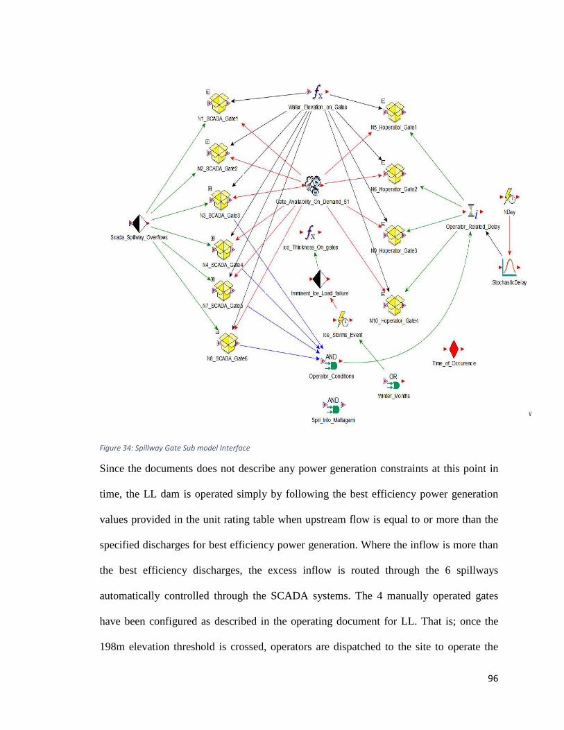
96
Figure 34: Spillway Gate Sub model Interface
Since the documents does not describe any power generation constraints at this point in
time, the LL dam is operated simply by following the best efficiency power generation
values provided in the unit rating table when upstream flow is equal to or more than the
specified discharges for best efficiency power generation. Where the inflow is more than
the best efficiency discharges, the excess inflow is routed through the 6 spillways
automatically controlled through the SCADA systems. The 4 manually operated gates
have been configured as described in the operating document for LL. That is; once the
198m elevation threshold is crossed, operators are dispatched to the site to operate the
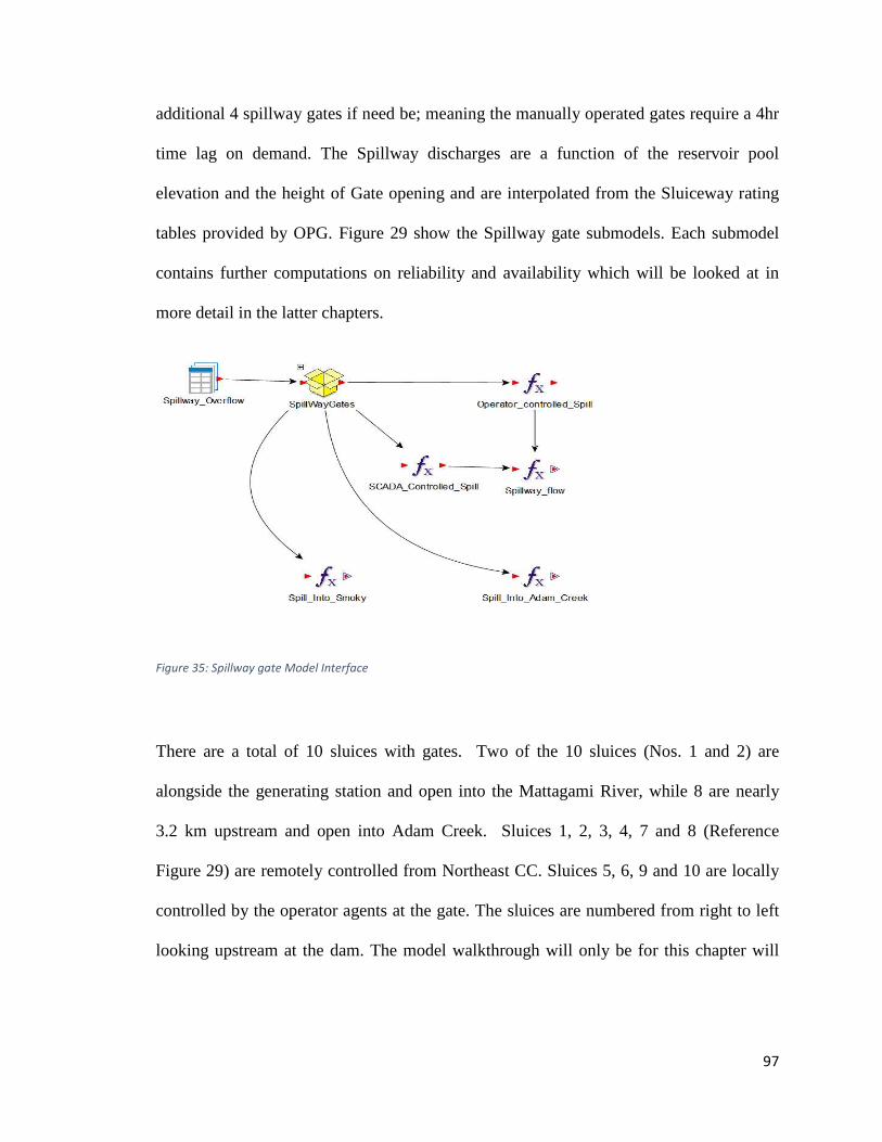
97
additional 4 spillway gates if need be; meaning the manually operated gates require a 4hr
time lag on demand. The Spillway discharges are a function of the reservoir pool
elevation and the height of Gate opening and are interpolated from the Sluiceway rating
tables provided by OPG. Figure 29 show the Spillway gate submodels. Each submodel
contains further computations on reliability and availability which will be looked at in
more detail in the latter chapters.
Figure 35: Spillway gate Model Interface
There are a total of 10 sluices with gates. Two of the 10 sluices (Nos. 1 and 2) are
alongside the generating station and open into the Mattagami River, while 8 are nearly
3.2 km upstream and open into Adam Creek. Sluices 1, 2, 3, 4, 7 and 8 (Reference
Figure 29) are remotely controlled from Northeast CC. Sluices 5, 6, 9 and 10 are locally
controlled by the operator agents at the gate. The sluices are numbered from right to left
looking upstream at the dam. The model walkthrough will only be for this chapter will
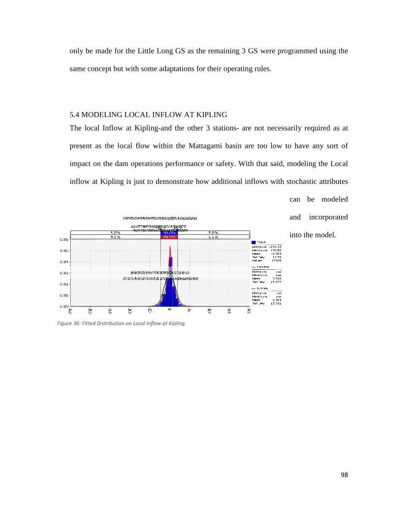
98
only be made for the Little Long GS as the remaining 3 GS were programmed using the
same concept but with some adaptations for their operating rules.
5.4 MODELING LOCAL INFLOW AT KIPLING
The local Inflow at Kipling-and the other 3 stations- are not necessarily required as at
present as the local flow within the Mattagami basin are too low to have any sort of
impact on the dam operations performance or safety. With that said, modeling the Local
inflow at Kipling is just to demonstrate how additional inflows with stochastic attributes
can be modeled
and incorporated
into the model.
Figure 36: Fitted Distribution on Local Inflow at Kipling
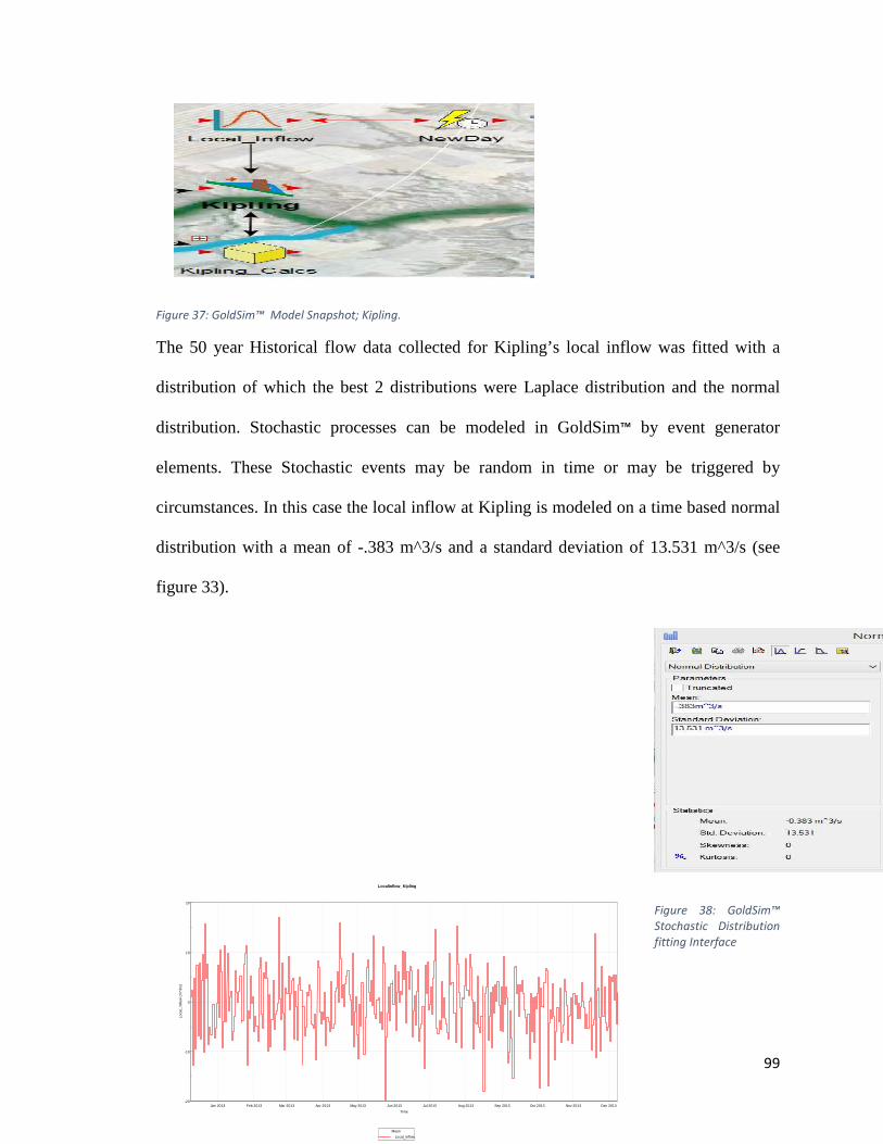
99
Figure 37: GoldSim™ Model Snapshot; Kipling.
The 50 year Historical flow data collected for Kipling’s local inflow was fitted with a
distribution of which the best 2 distributions were Laplace distribution and the normal
distribution. Stochastic processes can be modeled in GoldSim™ by event generator
elements. These Stochastic events may be random in time or may be triggered by
circumstances. In this case the local inflow at Kipling is modeled on a time based normal
distribution with a mean of -.383 m^3/s and a standard deviation of 13.531 m^3/s (see
figure 33).
Figure 38: GoldSim™
Stochastic Distribution
fitting Interface
-20
-10
0
10
20
Jan 2013 Feb 2013 Mar 2013 Apr 2013 May 2013 Jun 2013 Jul 2013 Aug 2013 Sep 2013 Oct 2013 Nov 2013 Dec 2013
Loca
l_In
flow
(m
^3/s
)
Time
LocalInflow_Kipling
Mean
Local_Inflow
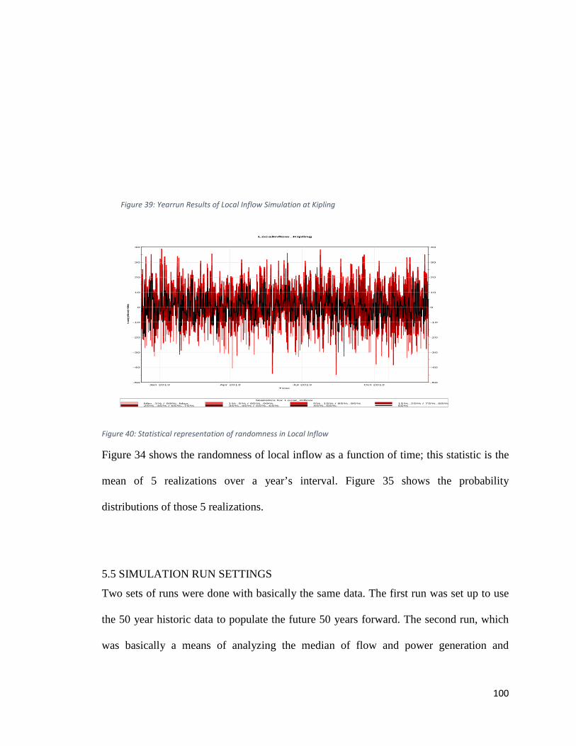
100
Figure 40: Statistical representation of randomness in Local Inflow
Figure 34 shows the randomness of local inflow as a function of time; this statistic is the
mean of 5 realizations over a year’s interval. Figure 35 shows the probability
distributions of those 5 realizations.
5.5 SIMULATION RUN SETTINGS
Two sets of runs were done with basically the same data. The first run was set up to use
the 50 year historic data to populate the future 50 years forward. The second run, which
was basically a means of analyzing the median of flow and power generation and
-50
-40
-30
-20
-10
0
10
20
30
40
Jan 2013 Apr 2013 Jul 2013 Oct 2013
Local_Inflow (m̂
3/s)
Time
-50
-40
-30
-20
-10
0
10
20
30
40
LocalInflow_Kipling
Statistics for Local_Inflow
Min..1% / 99%..Max 1%..5% / 95%..99% 5%..15% / 85%..95% 15%..25% / 75%..85%25%..35% / 65%..75% 35%..45% / 55%..65% 45%..55% 50%
Figure 39: Yearrun Results of Local Inflow Simulation at Kipling
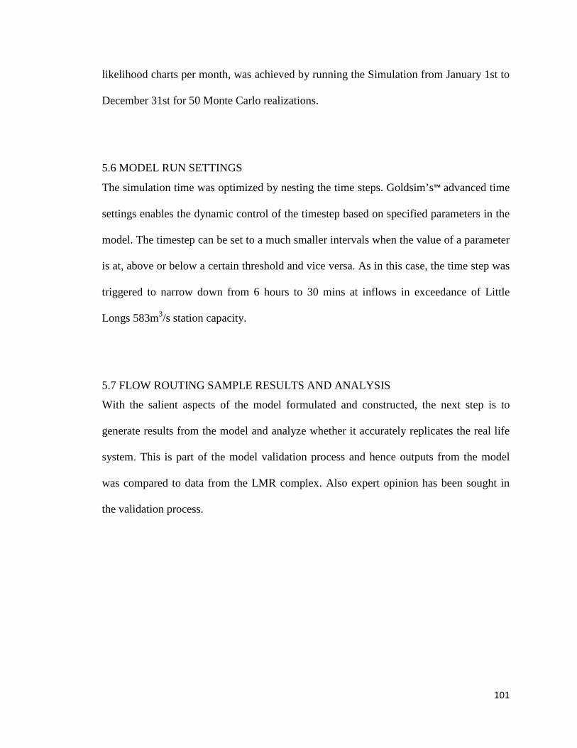
101
likelihood charts per month, was achieved by running the Simulation from January 1st to
December 31st for 50 Monte Carlo realizations.
5.6 MODEL RUN SETTINGS
The simulation time was optimized by nesting the time steps. Goldsim’s™ advanced time
settings enables the dynamic control of the timestep based on specified parameters in the
model. The timestep can be set to a much smaller intervals when the value of a parameter
is at, above or below a certain threshold and vice versa. As in this case, the time step was
triggered to narrow down from 6 hours to 30 mins at inflows in exceedance of Little
Longs 583m3/s station capacity.
5.7 FLOW ROUTING SAMPLE RESULTS AND ANALYSIS
With the salient aspects of the model formulated and constructed, the next step is to
generate results from the model and analyze whether it accurately replicates the real life
system. This is part of the model validation process and hence outputs from the model
was compared to data from the LMR complex. Also expert opinion has been sought in
the validation process.
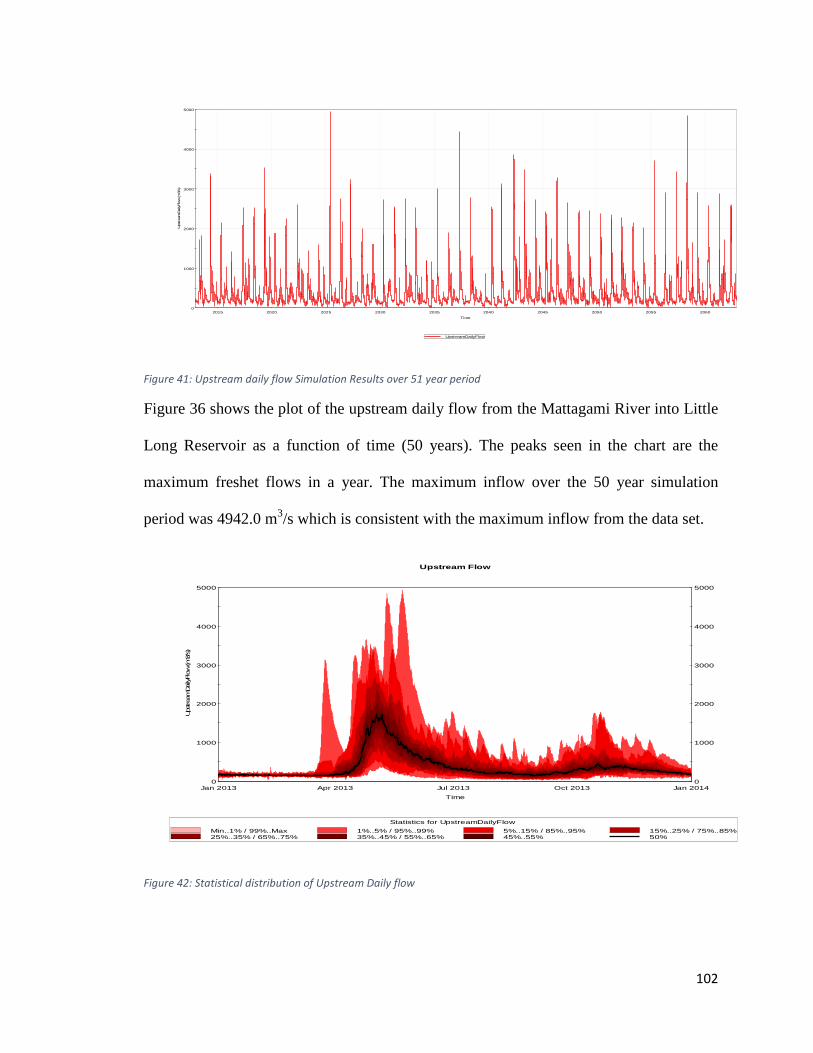
102
Figure 41: Upstream daily flow Simulation Results over 51 year period
Figure 36 shows the plot of the upstream daily flow from the Mattagami River into Little
Long Reservoir as a function of time (50 years). The peaks seen in the chart are the
maximum freshet flows in a year. The maximum inflow over the 50 year simulation
period was 4942.0 m3/s which is consistent with the maximum inflow from the data set.
Figure 42: Statistical distribution of Upstream Daily flow
0
1000
2000
3000
4000
5000
2015 2020 2025 2030 2035 2040 2045 2050 2055 2060
Ups
trea
mDai
lyFlo
w (m
3/s)
Time
UpstreamDailyFlow
0
1000
2000
3000
4000
5000
Jan 2013 Apr 2013 Jul 2013 Oct 2013 Jan 2014
Ups
trea
mDailyFlow (m3/s)
Time
0
1000
2000
3000
4000
5000
Upstream Flow
Statistics for UpstreamDailyFlow
Min..1% / 99%..Max 1%..5% / 95%..99% 5%..15% / 85%..95% 15%..25% / 75%..85%25%..35% / 65%..75% 35%..45% / 55%..65% 45%..55% 50%
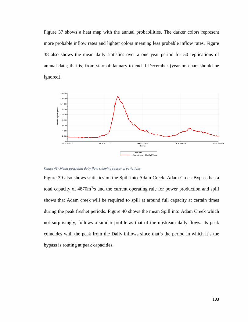
103
Figure 37 shows a heat map with the annual probabilities. The darker colors represent
more probable inflow rates and lighter colors meaning less probable inflow rates. Figure
38 also shows the mean daily statistics over a one year period for 50 replications of
annual data; that is, from start of January to end if December (year on chart should be
ignored).
Figure 43: Mean upstream daily flow showing seasonal variations
Figure 39 also shows statistics on the Spill into Adam Creek. Adam Creek Bypass has a
total capacity of 4870m3/s and the current operating rule for power production and spill
shows that Adam creek will be required to spill at around full capacity at certain times
during the peak freshet periods. Figure 40 shows the mean Spill into Adam Creek which
not surprisingly, follows a similar profile as that of the upstream daily flows. Its peak
coincides with the peak from the Daily inflows since that’s the period in which it’s the
bypass is routing at peak capacities.
0
200
400
600
800
1000
1200
1400
1600
1800
Jan 2013 Apr 2013 Jul 2013 Oct 2013 Jan 2014
Ups
trea
mDailyFlow (m3/s)
Time
Mean
UpstreamDailyFlow
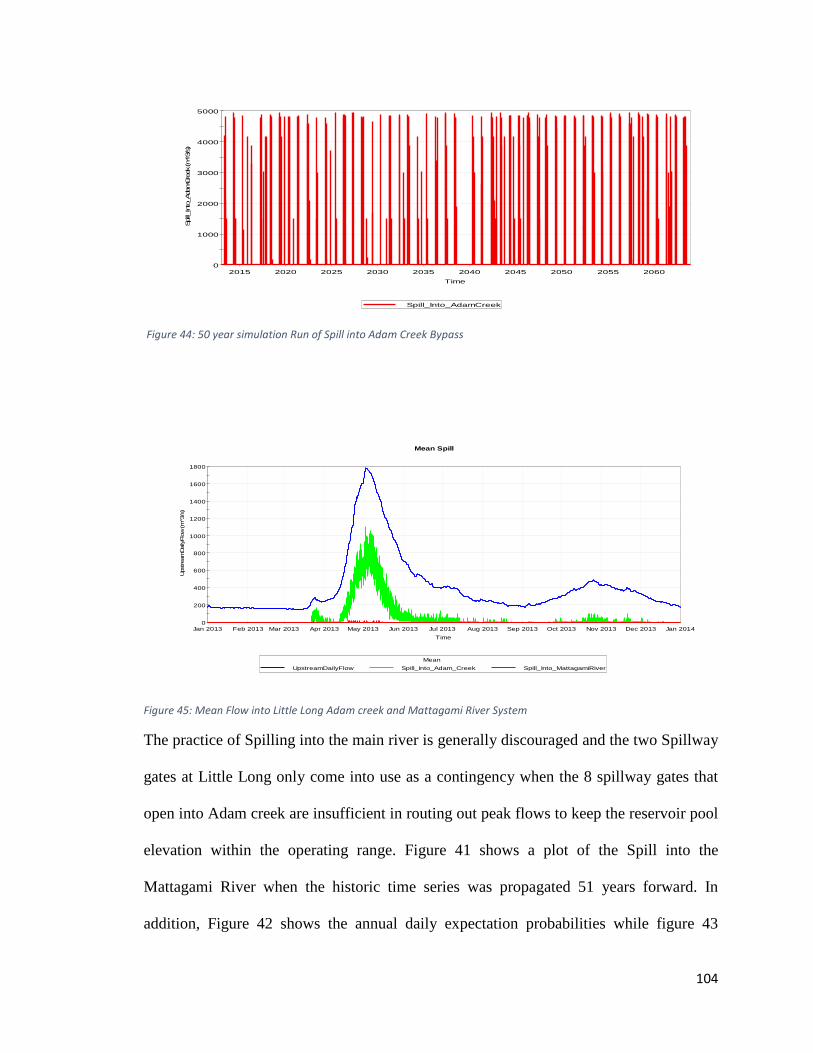
104
Figure 45: Mean Flow into Little Long Adam creek and Mattagami River System
The practice of Spilling into the main river is generally discouraged and the two Spillway
gates at Little Long only come into use as a contingency when the 8 spillway gates that
open into Adam creek are insufficient in routing out peak flows to keep the reservoir pool
elevation within the operating range. Figure 41 shows a plot of the Spill into the
Mattagami River when the historic time series was propagated 51 years forward. In
addition, Figure 42 shows the annual daily expectation probabilities while figure 43
0
200
400
600
800
1000
1200
1400
1600
1800
Jan 2013 Feb 2013 Mar 2013 Apr 2013 May 2013 Jun 2013 Jul 2013 Aug 2013 Sep 2013 Oct 2013 Nov 2013 Dec 2013 Jan 2014
Ups
trea
mDai
lyFlo
w (m̂
3/s)
Time
Mean Spill
Mean
UpstreamDailyFlow Spill_Into_Adam_Creek Spill_Into_MattagamiRiver
0
1000
2000
3000
4000
5000
2015 2020 2025 2030 2035 2040 2045 2050 2055 2060
Spill_
Into_A
damCre
ek (m̂
3/s)
Time
Spill_Into_AdamCreek
Figure 44: 50 year simulation Run of Spill into Adam Creek Bypass
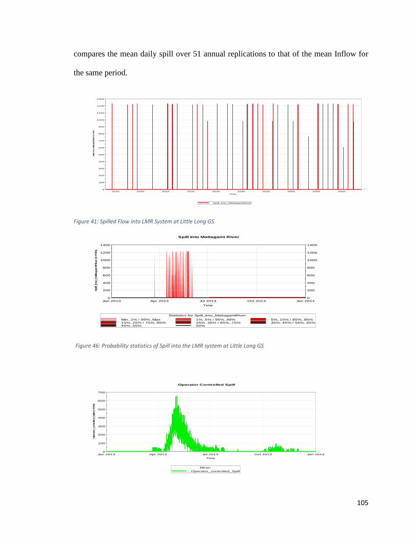
105
compares the mean daily spill over 51 annual replications to that of the mean Inflow for
the same period.
Figure 41: Spilled Flow into LMR System at Little Long GS
0
100
200
300
400
500
600
700
800
900
1000
1100
1200
1300
2015 2020 2025 2030 2035 2040 2045 2050 2055 2060
Spill_Into_M
attag
amiRiver (m̂
3/s)
Time
Spill_Into_MattagamiRiver
0
200
400
600
800
1000
1200
1400
Jan 2013 Apr 2013 Jul 2013 Oct 2013 Jan 2014
Spill_Into_M
atta
gamiRiver (m̂
3/s)
Time
0
200
400
600
800
1000
1200
1400
Spill Into Mattagami River
Statistics for Spill_Into_MattagamiRiver
Min..1% / 99%..Max 1%..5% / 95%..99% 5%..15% / 85%..95%15%..25% / 75%..85% 25%..35% / 65%..75% 35%..45% / 55%..65%45%..55% 50%
0
100
200
300
400
500
600
700
Jan 2013 Apr 2013 Jul 2013 Oct 2013 Jan 2014
Ope
rator_co
ntrolle
d_Spill (m̂
3/s)
Time
Operator Controlled Spill
Mean
Operator_controlled_Spill
Figure 46: Probability statistics of Spill into the LMR system at Little Long GS
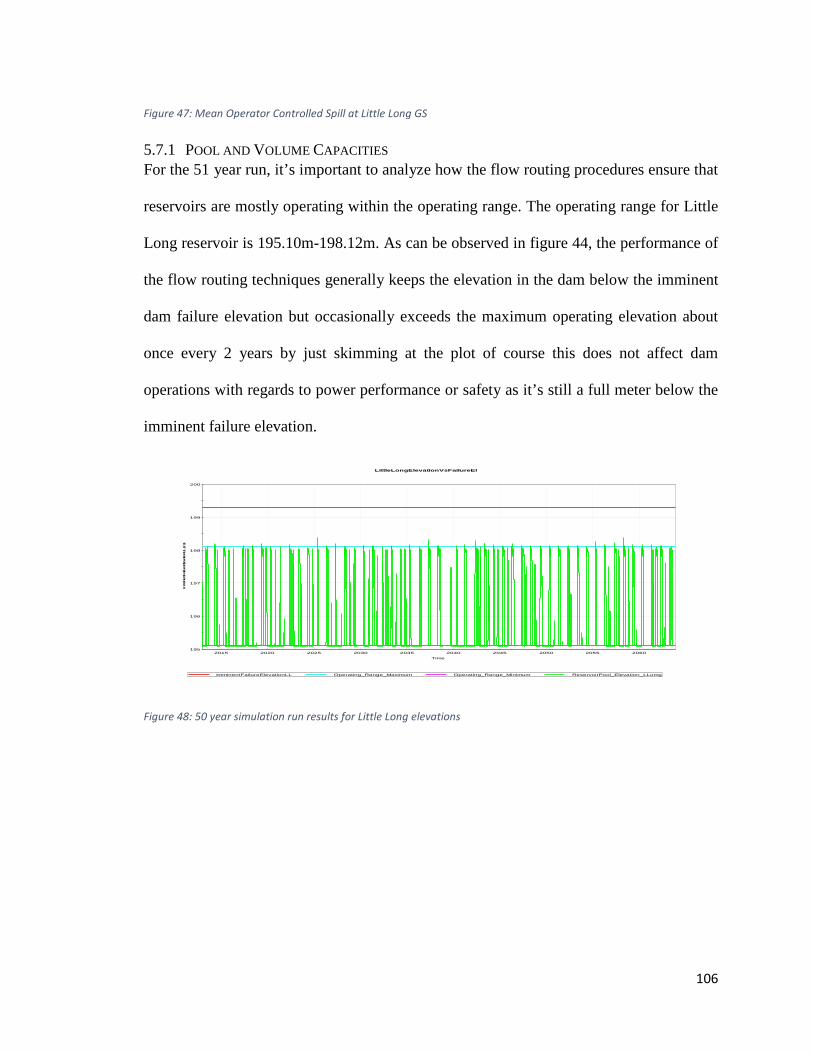
106
5.7.1 POOL AND VOLUME CAPACITIES For the 51 year run, it’s important to analyze how the flow routing procedures ensure that
reservoirs are mostly operating within the operating range. The operating range for Little
Long reservoir is 195.10m-198.12m. As can be observed in figure 44, the performance of
the flow routing techniques generally keeps the elevation in the dam below the imminent
dam failure elevation but occasionally exceeds the maximum operating elevation about
once every 2 years by just skimming at the plot of course this does not affect dam
operations with regards to power performance or safety as it’s still a full meter below the
imminent failure elevation.
Figure 48: 50 year simulation run results for Little Long elevations
195
196
197
198
199
200
2015 2020 2025 2030 2035 2040 2045 2050 2055 2060
Imminen
tFailureElevationLL
(m)
Time
LittleLongElevationVsFailureEl
ImminentFailureElevationLL Operating_Range_Maximum Operating_Range_Minimum ReservoirPool_Elevation_LLomg
Figure 47: Mean Operator Controlled Spill at Little Long GS
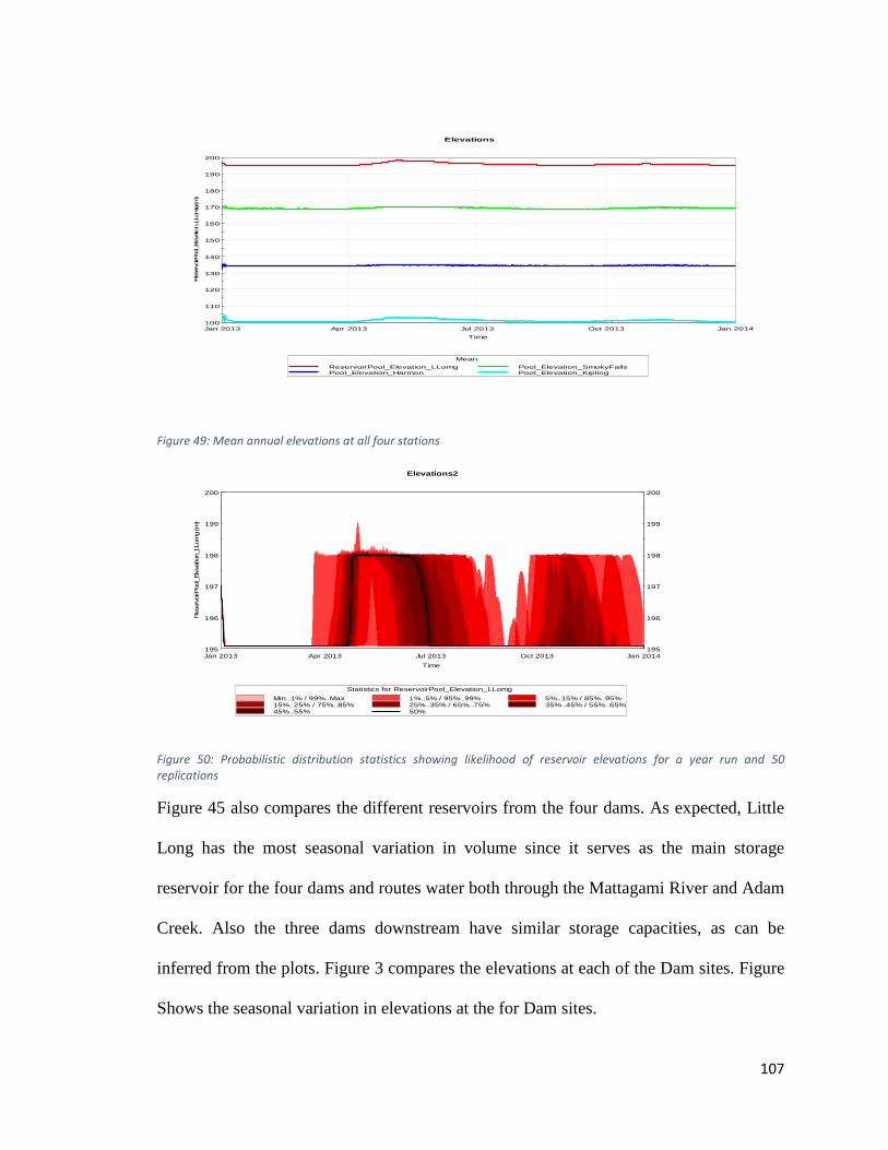
107
Figure 49: Mean annual elevations at all four stations
Figure 50: Probabilistic distribution statistics showing likelihood of reservoir elevations for a year run and 50
replications
Figure 45 also compares the different reservoirs from the four dams. As expected, Little
Long has the most seasonal variation in volume since it serves as the main storage
reservoir for the four dams and routes water both through the Mattagami River and Adam
Creek. Also the three dams downstream have similar storage capacities, as can be
inferred from the plots. Figure 3 compares the elevations at each of the Dam sites. Figure
Shows the seasonal variation in elevations at the for Dam sites.
195
196
197
198
199
200
Jan 2013 Apr 2013 Jul 2013 Oct 2013 Jan 2014
Res
ervo
irPoo
l_Ele
vatio
n_LL
omg
(m)
Time
195
196
197
198
199
200
Elevations2
Statistics for ReservoirPool_Elevation_LLomg
Min..1% / 99%..Max 1%..5% / 95%..99% 5%..15% / 85%..95%15%..25% / 75%..85% 25%..35% / 65%..75% 35%..45% / 55%..65%45%..55% 50%
100
110
120
130
140
150
160
170
180
190
200
Jan 2013 Apr 2013 Jul 2013 Oct 2013 Jan 2014
Res
ervo
irPoo
l_Eleva
tion_L
Lomg (m
)
Time
Elevations
Mean
ReservoirPool_Elevation_LLomg Pool_Elevation_SmokyFallsPool_Elevation_Harmon Pool_Elevation_Kipling
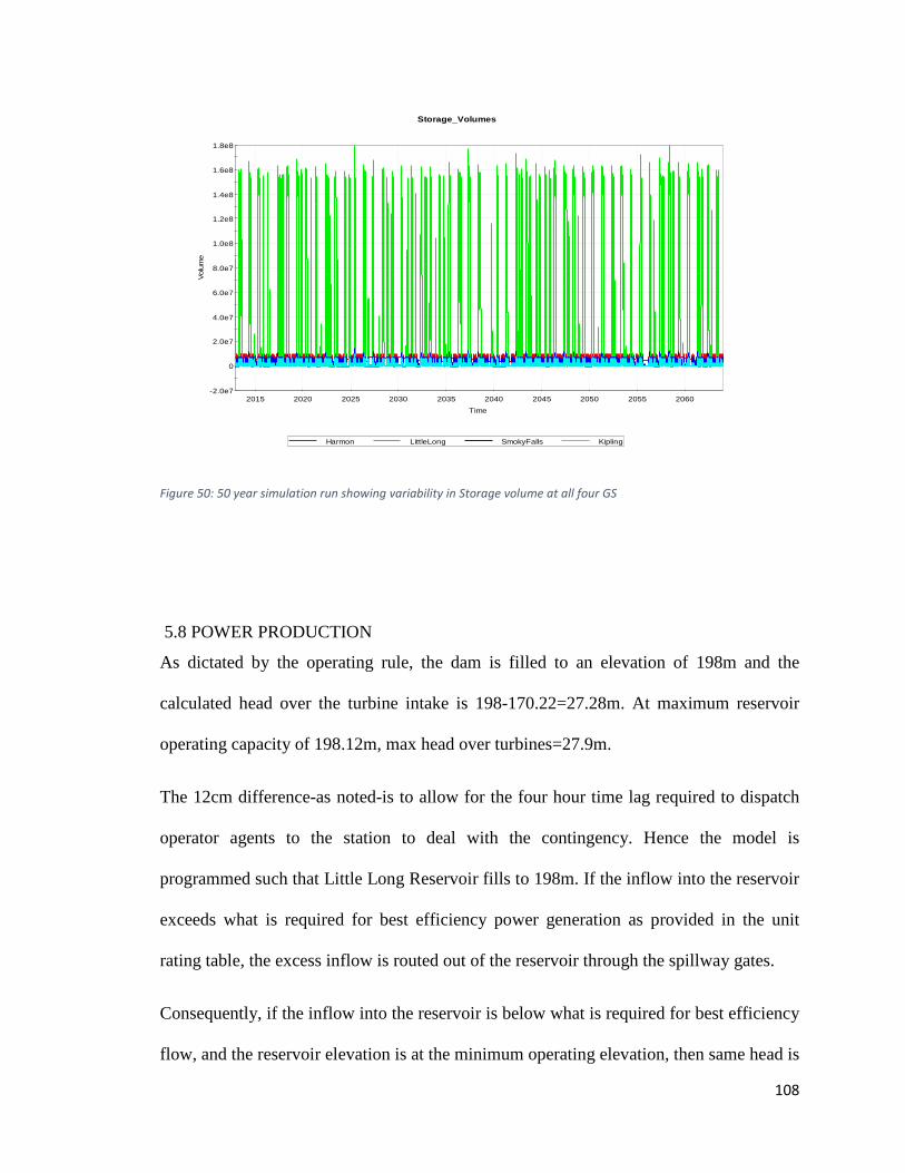
108
Figure 50: 50 year simulation run showing variability in Storage volume at all four GS
5.8 POWER PRODUCTION
As dictated by the operating rule, the dam is filled to an elevation of 198m and the
calculated head over the turbine intake is 198-170.22=27.28m. At maximum reservoir
operating capacity of 198.12m, max head over turbines=27.9m.
The 12cm difference-as noted-is to allow for the four hour time lag required to dispatch
operator agents to the station to deal with the contingency. Hence the model is
programmed such that Little Long Reservoir fills to 198m. If the inflow into the reservoir
exceeds what is required for best efficiency power generation as provided in the unit
rating table, the excess inflow is routed out of the reservoir through the spillway gates.
Consequently, if the inflow into the reservoir is below what is required for best efficiency
flow, and the reservoir elevation is at the minimum operating elevation, then same head is
-2.0e7
0
2.0e7
4.0e7
6.0e7
8.0e7
1.0e8
1.2e8
1.4e8
1.6e8
1.8e8
2015 2020 2025 2030 2035 2040 2045 2050 2055 2060
Volu
me
Time
Storage_Volumes
Harmon LittleLong SmokyFalls Kipling

109
maintained while inflow water (equivalent volume) is routed through turbine intake
sluices. On the other hand if the inflow into the reservoir is less than the minimum for
best efficiency flow but the reservoir elevation is above the minimum operating
elevation, then the reservoir elevation is gradually lowered while generating the
minimum best efficiency power until the minimum operating threshold is crossed.

110
Since the Power Generation documents does not describe any power generation
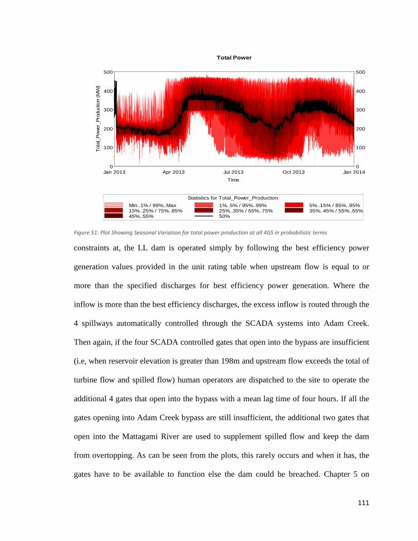
111
constraints at, the LL dam is operated simply by following the best efficiency power
generation values provided in the unit rating table when upstream flow is equal to or
more than the specified discharges for best efficiency power generation. Where the
inflow is more than the best efficiency discharges, the excess inflow is routed through the
4 spillways automatically controlled through the SCADA systems into Adam Creek.
Then again, if the four SCADA controlled gates that open into the bypass are insufficient
(i.e, when reservoir elevation is greater than 198m and upstream flow exceeds the total of
turbine flow and spilled flow) human operators are dispatched to the site to operate the
additional 4 gates that open into the bypass with a mean lag time of four hours. If all the
gates opening into Adam Creek bypass are still insufficient, the additional two gates that
open into the Mattagami River are used to supplement spilled flow and keep the dam
from overtopping. As can be seen from the plots, this rarely occurs and when it has, the
gates have to be available to function else the dam could be breached. Chapter 5 on
0
100
200
300
400
500
Jan 2013 Apr 2013 Jul 2013 Oct 2013 Jan 2014
Tot
al_P
ower
_Pro
duct
ion
(MW
)
Time
0
100
200
300
400
500
Total Power
Statistics for Total_Power_Production
Min..1% / 99%..Max 1%..5% / 95%..99% 5%..15% / 85%..95%15%..25% / 75%..85% 25%..35% / 65%..75% 35%..45% / 55%..65%45%..55% 50%
Figure 51: Plot Showing Seasonal Variation for total power production at all 4GS in probabilistic terms
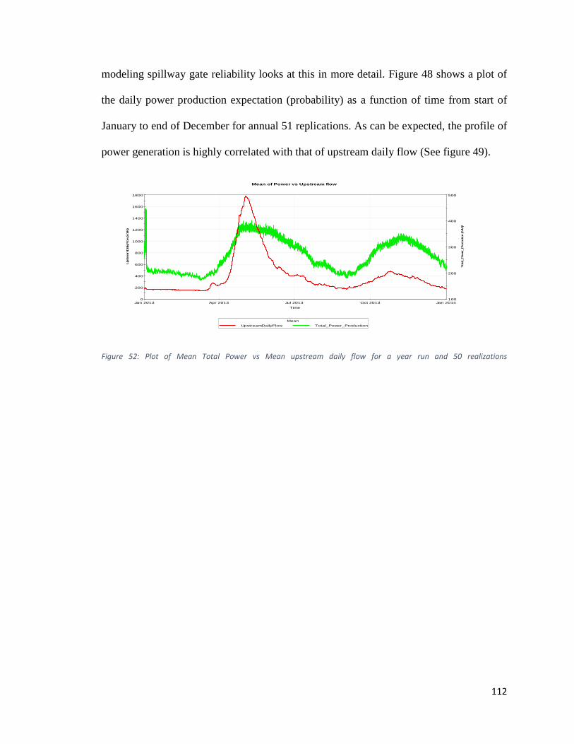
112
modeling spillway gate reliability looks at this in more detail. Figure 48 shows a plot of
the daily power production expectation (probability) as a function of time from start of
January to end of December for annual 51 replications. As can be expected, the profile of
power generation is highly correlated with that of upstream daily flow (See figure 49).
Figure 52: Plot of Mean Total Power vs Mean upstream daily flow for a year run and 50 realizations
0
200
400
600
800
1000
1200
1400
1600
1800
Jan 2013 Apr 2013 Jul 2013 Oct 2013 Jan 2014
Ups
trea
mDailyFlow (m3/s)
Time
100
200
300
400
500
Total_P
ower
_Pro
duction (M
W)
Mean of Power vs Upstream flow
Mean
UpstreamDailyFlow Total_Power_Production
113
6. SPILLWAY ANALYSIS MODELING AND RELIABILITY ANALYSIS
The main function of Spilway gates at dam sites is to safely pass water from one point to
another; usually from a reservoir, through a dam to a downstream river or reservoir This
is achieved by keeping the 3 main components, namely: the rate of flow, the physical
conveyance of flow and the kinetic and potential energy of the flow under control.
According to Baecher et al, “The components of water conduits are all natural or
manmade structures with civil, mechanical or electrical functions and with certain
capabilities to resist the dynamic and static loads imposed on them”. Meaning for a
spillway to perform it’s task safely, flow must be kept to within a range which does not
exceed the design capacities of it’s subcomponents (electrical, structual, mechanical etc.).
Thus, the reliable peformance of a Spillway system is both a function of time and the
loads placed upon upon it. This chapter explores the dynamics of flow routing though
Spillway gates and the inherent reliability of these gates under extreme flow and normal
flow conditions over time. The Mattagami river case study herein will be used as the
model example for demonstrating how flow is routed through Spillway gates and their
inherent reliability.
6.1 VERTICAL LIFT GATES
Vertical lift gates are a common type of dam gate. They are used in many different
applications including spillways, control towers, and regulating outlets. Machinery
typically is located on a structural feature above the gate. For most dam applications,
vertical lift gates must be operated under differential head conditions. The differential
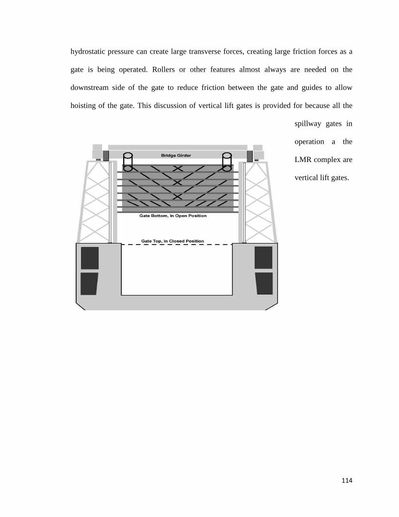
114
hydrostatic pressure can create large transverse forces, creating large friction forces as a
gate is being operated. Rollers or other features almost always are needed on the
downstream side of the gate to reduce friction between the gate and guides to allow
hoisting of the gate. This discussion of vertical lift gates is provided for because all the
spillway gates in
operation a the
LMR complex are
vertical lift gates.
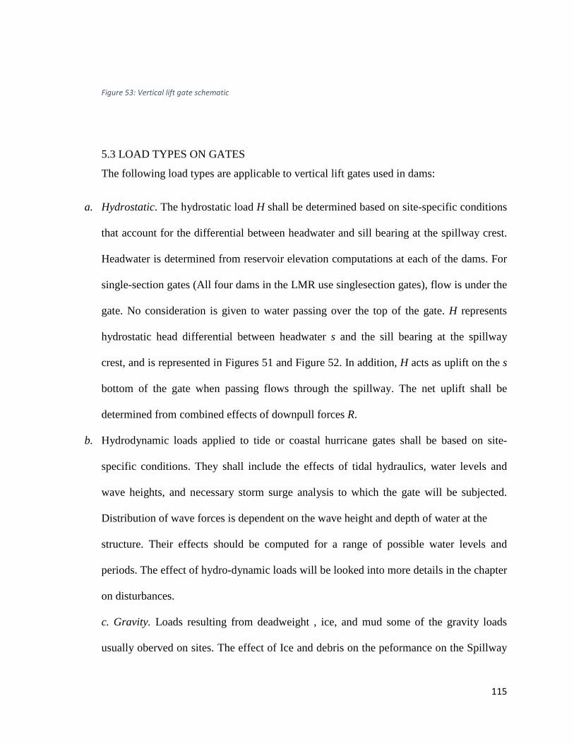
115
Figure 53: Vertical lift gate schematic
5.3 LOAD TYPES ON GATES
The following load types are applicable to vertical lift gates used in dams:
a. Hydrostatic. The hydrostatic load H shall be determined based on site-specific conditions
that account for the differential between headwater and sill bearing at the spillway crest.
Headwater is determined from reservoir elevation computations at each of the dams. For
single-section gates (All four dams in the LMR use singlesection gates), flow is under the
gate. No consideration is given to water passing over the top of the gate. H represents
hydrostatic head differential between headwater s and the sill bearing at the spillway
crest, and is represented in Figures 51 and Figure 52. In addition, H acts as uplift on the s
bottom of the gate when passing flows through the spillway. The net uplift shall be
determined from combined effects of downpull forces R.
b. Hydrodynamic loads applied to tide or coastal hurricane gates shall be based on site-
specific conditions. They shall include the effects of tidal hydraulics, water levels and
wave heights, and necessary storm surge analysis to which the gate will be subjected.
Distribution of wave forces is dependent on the wave height and depth of water at the
structure. Their effects should be computed for a range of possible water levels and
periods. The effect of hydro-dynamic loads will be looked into more details in the chapter
on disturbances.
c. Gravity. Loads resulting from deadweight , ice, and mud some of the gravity loads
usually oberved on sites. The effect of Ice and debris on the peformance on the Spillway
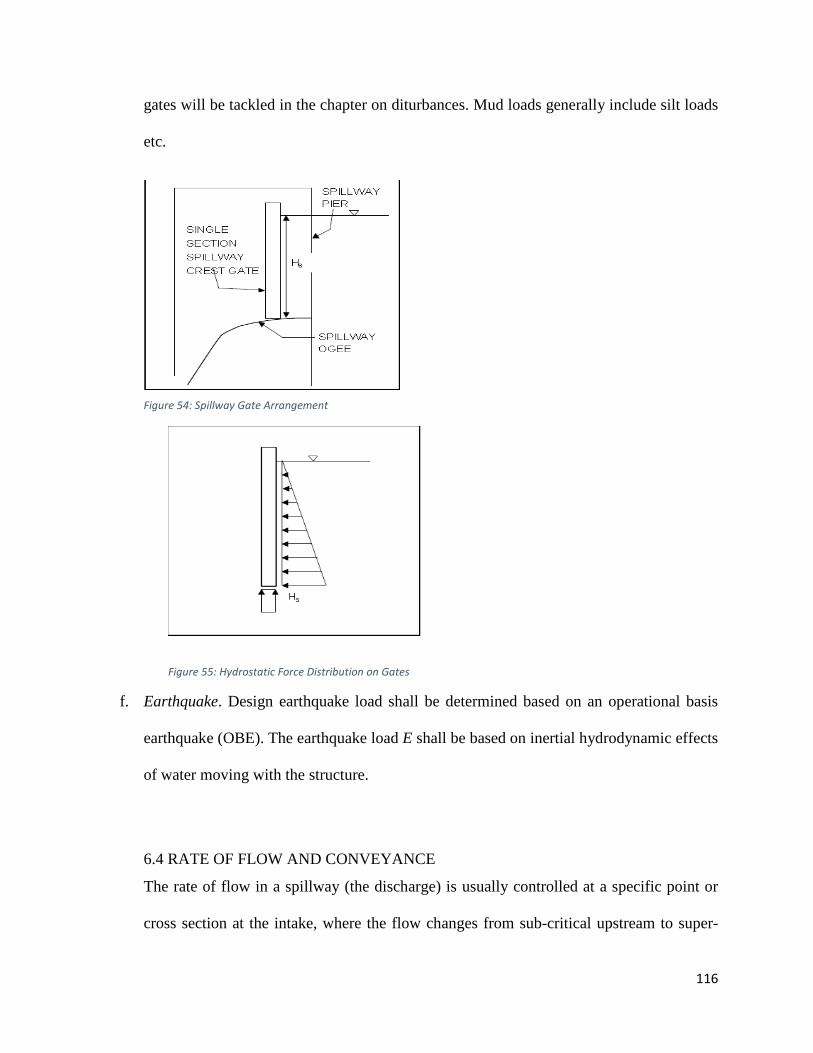
116
gates will be tackled in the chapter on diturbances. Mud loads generally include silt loads
etc.
Figure 55: Hydrostatic Force Distribution on Gates
f. Earthquake. Design earthquake load shall be determined based on an operational basis
earthquake (OBE). The earthquake load E shall be based on inertial hydrodynamic effects
of water moving with the structure.
6.4 RATE OF FLOW AND CONVEYANCE
The rate of flow in a spillway (the discharge) is usually controlled at a specific point or
cross section at the intake, where the flow changes from sub-critical upstream to super-
Figure 54: Spillway Gate Arrangement
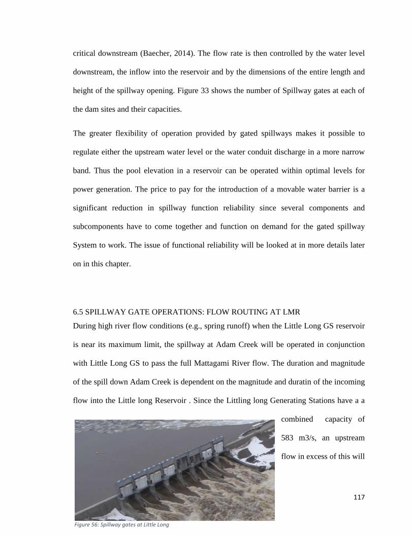
117
critical downstream (Baecher, 2014). The flow rate is then controlled by the water level
downstream, the inflow into the reservoir and by the dimensions of the entire length and
height of the spillway opening. Figure 33 shows the number of Spillway gates at each of
the dam sites and their capacities.
The greater flexibility of operation provided by gated spillways makes it possible to
regulate either the upstream water level or the water conduit discharge in a more narrow
band. Thus the pool elevation in a reservoir can be operated within optimal levels for
power generation. The price to pay for the introduction of a movable water barrier is a
significant reduction in spillway function reliability since several components and
subcomponents have to come together and function on demand for the gated spillway
System to work. The issue of functional reliability will be looked at in more details later
on in this chapter.
6.5 SPILLWAY GATE OPERATIONS: FLOW ROUTING AT LMR
During high river flow conditions (e.g., spring runoff) when the Little Long GS reservoir
is near its maximum limit, the spillway at Adam Creek will be operated in conjunction
with Little Long GS to pass the full Mattagami River flow. The duration and magnitude
of the spill down Adam Creek is dependent on the magnitude and duratin of the incoming
flow into the Little long Reservoir . Since the Littling long Generating Stations have a a
combined capacity of
583 m3/s, an upstream
flow in excess of this will
Figure 56: Spillway gates at Little Long
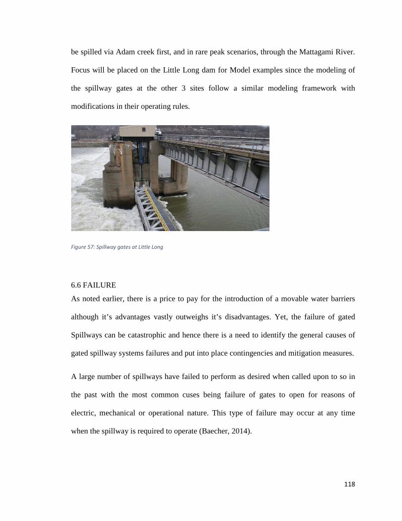
118
be spilled via Adam creek first, and in rare peak scenarios, through the Mattagami River.
Focus will be placed on the Little Long dam for Model examples since the modeling of
the spillway gates at the other 3 sites follow a similar modeling framework with
modifications in their operating rules.
Figure 57: Spillway gates at Little Long
6.6 FAILURE
As noted earlier, there is a price to pay for the introduction of a movable water barriers
although it’s advantages vastly outweighs it’s disadvantages. Yet, the failure of gated
Spillways can be catastrophic and hence there is a need to identify the general causes of
gated spillway systems failures and put into place contingencies and mitigation measures.
A large number of spillways have failed to perform as desired when called upon to so in
the past with the most common cuses being failure of gates to open for reasons of
electric, mechanical or operational nature. This type of failure may occur at any time
when the spillway is required to operate (Baecher, 2014).

119
6.7 FAILURE MECHANISMS
Leveson (1995) defined failure as the nonperformance or inability of the system or
component to perform its intended function for a specified time under specified
environmental conditions. Failure conditions are usually brought about by any one of a
number of natural hazards or other external or internal disturbances, but eventually,
failure always comes down to structural insufficiency, either insufficient dimensions to
contain the flow or insufficient integrity to withstand the occurring forces or a
combination of these (Baecher, 2014). At a high level of abstraction any occasion when a
system does not fulfil its function constitutes a failure of the system.
Failure at a systems level differs from failure at the component level in that failure at the
component level may not necessarily cause failure of the entire system. In some cases, a
system may still function even though it has a component failure and in fact this is a
property of a well designed system (Baecher, 2014). The high level definition is not
usually sufficient for the purpose of a detailed analysis of the system, but the failure
needs to be tied to a particular component or set of components, whether physical objects,
resources or procedures. This concept will be explored later on in this chapter with the
aim of modeling how component and subcomponent failure affects the entire system at a
higher level. For example, a spillway gate might not open on demand due to an electrical
issue related to it’s generator but the other spillway gates may function and the entire
system may be unaffected by the failure of one of the subcomponents f that particular
spillway gate. It is up to the user to define which particular definition of failure and
failure categories best serve the purpose of his analysis.
120
6.8 FAILURE MODE OF GATES
a. Hydraulic capacity: Insufficient hydraulic capacity of the spillway gates is the classic
failure mode that will be explored. It will (may) manifest itself as a raised reservoir
water level and the final failure may then take on the form of a dam overtopping.
b. Potential capacity not available: The hydraulic capacity of spillway gates may be reduced
by the influence of floating debris, ice or sediments restricting the free opening size or by
gates not opening.
c. Floating debris: Rivers will carry floating debris, especially during floods. Depending on
the natural conditions of the catchment the debris may be in the form of uprooted large
trees, cut timber, branches, bushes, grass, floating mires, dead animals and various
manmade objects such as bridges, boats and houses. Floating debris can significantly
influence the discharge capacity of spillways by sticking to structures such as gates,
spillway piers and bridges spanning spillways, to obstruct spillway openings and prevent
gate operation (Baecher, 2014). This phenomenon will be further explored in the chapter
on disturbances.
d. Ice: Ice can reduce spillway discharge capacities in different ways. At break-up of lake
ice or river ice and the ensuing ice floes can build up and jam spillway openings,
particularly those of limited free dimensions in the same way as trees or other types of
floating debris. Ice or frazil developed in super-cooled water can also adhere to gates and
spillway piers and prevent gate opening or reduce the size of the free opening and thereby
limit the discharge capacity. Leaky seals are a not uncommon reason for ice build-up
between gates and piers.

121
Ice jams, many meters in height, can also develop where frazil adheres to the boundaries
of rivers and channels to completely change the hydraulic capacities and rating curves.
Fresh water only requires super-cooling of the water to fractions of a degree under 0°
Celsius to make frazil production possible throughout a water body. Weather conditions
promoting super-cooling and frazil growth in shallow waters involve those with very high
heat losses from the water due to inter alia radiation, low air temperature, wind and heavy
snowfall. Where the effects of ice need to be considered specifically, modeling of the ice
conditions in the reservoir and river upstream and downstream may be required. Ideally
this should be done in coupled models taking into account the effects of the flow and
weather on the ice processes as well as the effects of the ice on the flow.
e. Sediments: Many rivers carry significant amounts of solids, especially those in more
easily erodible materials. In rivers running through old and stable igneous rocks,
sediments may on the contrary often not be present in appreciable amounts. Coarse
sediments, carried as bed load by a river will initially settle in the upstream end of
reservoirs, where flow velocities start to reduce and the carrying capacity of the flow
diminishes. Finer sediments carried as suspended load will continue further into a
reservoir and usually tends to create bars sloping around 1%. Unless regular (annual)
flushing is performed of the reservoir, these sediment bars may in time reach and start to
clog intake areas for water conduits, such as bottom outlets, power intakes and sometime
even spillway intakes. Sediments have a similar potential to disturb water conduit
operation as floating debris and ice, but in addition, the discharge of coarse sediments
may also lead to heavy erosion in the fast flowing water of low-level outlets.
122
6.9 RELIABILITY AND PEFORMANCE OF GATED SPILLWAYS
Gated Spillway systems are generally designed to set of defined engineering standards,
however with the effects of aging, exposure, preventative maintenance, and lack of
frequent operations in combination with human error seem to make these systems more
vulnerable than one would think (Baecher, 2014). The on demand failures of gated
Spillways are complex and may be caused by a gate component that can be repaired in
minutes to hours or a component that may cause complete failure of the gate system and
unexpected release of the reservoir containment.
6.9.1 FLOW ROUTING CAPACITIES Although the four GSs are in close proximity, Smoky Falls GS was constructed over 30
years earlier to serve a different purpose than Little Long GS, Harmon GS and Kipling
GS. Smoky Falls GS is a 4-unit, baseload station operating effectively 24 h/d with a rated
flow capacity of 188 m3/s. The other three stations (Little Long GS, Harmon GS and
Kipling GS) each has two units and are peaking stations that operate depending on
available inflows (Ontario Hydro 1990). The different operating patterns under the
current situation require that Smoky Falls GS, Harmon GS and Kipling GS headpond
water levels fluctuate daily.
6.9.2 MODELING FUNCTION AND FAILURE During the service life of a dam, operating conditions and natural environmental factors
may lead to some deterioration in its structural integrity, mechanical equipment, and
foundation. A fragility model of a dam provides a tool for rational safety assessment and
decision making by using a probabilistic framework to manage the various sources of
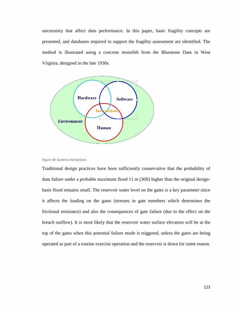
123
uncertainty that affect dam performance. In this paper, basic fragility concepts are
presented, and databases required to support the fragility assessment are identified. The
method is illustrated using a concrete monolith from the Bluestone Dam in West
Virginia, designed in the late 1930s.
Figure 58: Systems Interactions
Traditional design practices have been sufficiently conservative that the probability of
dam failure under a probable maximum flood 11 m (36ft) higher than the original design-
basis flood remains small. The reservoir water level on the gates is a key parameter since
it affects the loading on the gates (stresses in gate members which determines the
frictional resistance) and also the consequences of gate failure (due to the effect on the
breach outflow). It is most likely that the reservoir water surface elevation will be at the
top of the gates when this potential failure mode is triggered, unless the gates are being
operated as part of a routine exercise operation and the reservoir is down for some reason.
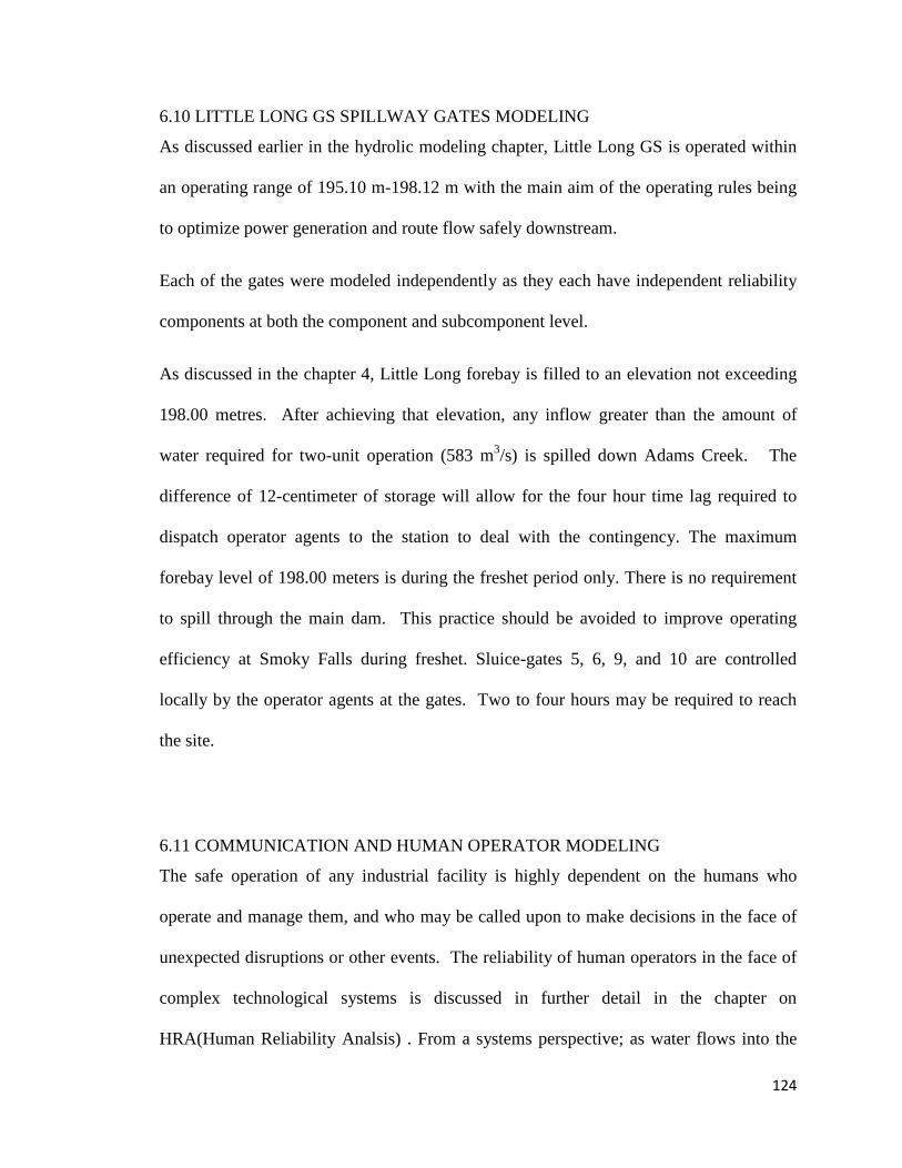
124
6.10 LITTLE LONG GS SPILLWAY GATES MODELING
As discussed earlier in the hydrolic modeling chapter, Little Long GS is operated within
an operating range of 195.10 m-198.12 m with the main aim of the operating rules being
to optimize power generation and route flow safely downstream.
Each of the gates were modeled independently as they each have independent reliability
components at both the component and subcomponent level.
As discussed in the chapter 4, Little Long forebay is filled to an elevation not exceeding
198.00 metres. After achieving that elevation, any inflow greater than the amount of
water required for two-unit operation (583 m3/s) is spilled down Adams Creek. The
difference of 12-centimeter of storage will allow for the four hour time lag required to
dispatch operator agents to the station to deal with the contingency. The maximum
forebay level of 198.00 meters is during the freshet period only. There is no requirement
to spill through the main dam. This practice should be avoided to improve operating
efficiency at Smoky Falls during freshet. Sluice-gates 5, 6, 9, and 10 are controlled
locally by the operator agents at the gates. Two to four hours may be required to reach
the site.
6.11 COMMUNICATION AND HUMAN OPERATOR MODELING
The safe operation of any industrial facility is highly dependent on the humans who
operate and manage them, and who may be called upon to make decisions in the face of
unexpected disruptions or other events. The reliability of human operators in the face of
complex technological systems is discussed in further detail in the chapter on
HRA(Human Reliability Analsis) . From a systems perspective; as water flows into the
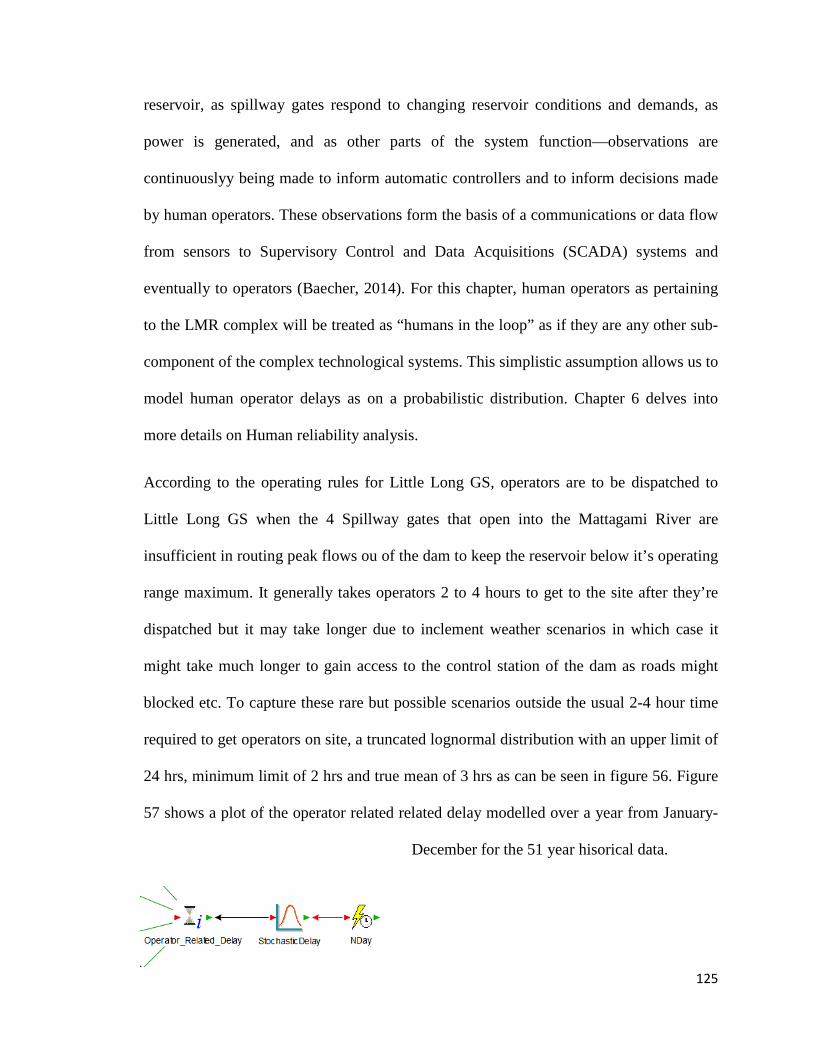
125
reservoir, as spillway gates respond to changing reservoir conditions and demands, as
power is generated, and as other parts of the system function—observations are
continuouslyy being made to inform automatic controllers and to inform decisions made
by human operators. These observations form the basis of a communications or data flow
from sensors to Supervisory Control and Data Acquisitions (SCADA) systems and
eventually to operators (Baecher, 2014). For this chapter, human operators as pertaining
to the LMR complex will be treated as “humans in the loop” as if they are any other sub-
component of the complex technological systems. This simplistic assumption allows us to
model human operator delays as on a probabilistic distribution. Chapter 6 delves into
more details on Human reliability analysis.
According to the operating rules for Little Long GS, operators are to be dispatched to
Little Long GS when the 4 Spillway gates that open into the Mattagami River are
insufficient in routing peak flows ou of the dam to keep the reservoir below it’s operating
range maximum. It generally takes operators 2 to 4 hours to get to the site after they’re
dispatched but it may take longer due to inclement weather scenarios in which case it
might take much longer to gain access to the control station of the dam as roads might
blocked etc. To capture these rare but possible scenarios outside the usual 2-4 hour time
required to get operators on site, a truncated lognormal distribution with an upper limit of
24 hrs, minimum limit of 2 hrs and true mean of 3 hrs as can be seen in figure 56. Figure
57 shows a plot of the operator related related delay modelled over a year from January-
December for the 51 year hisorical data.
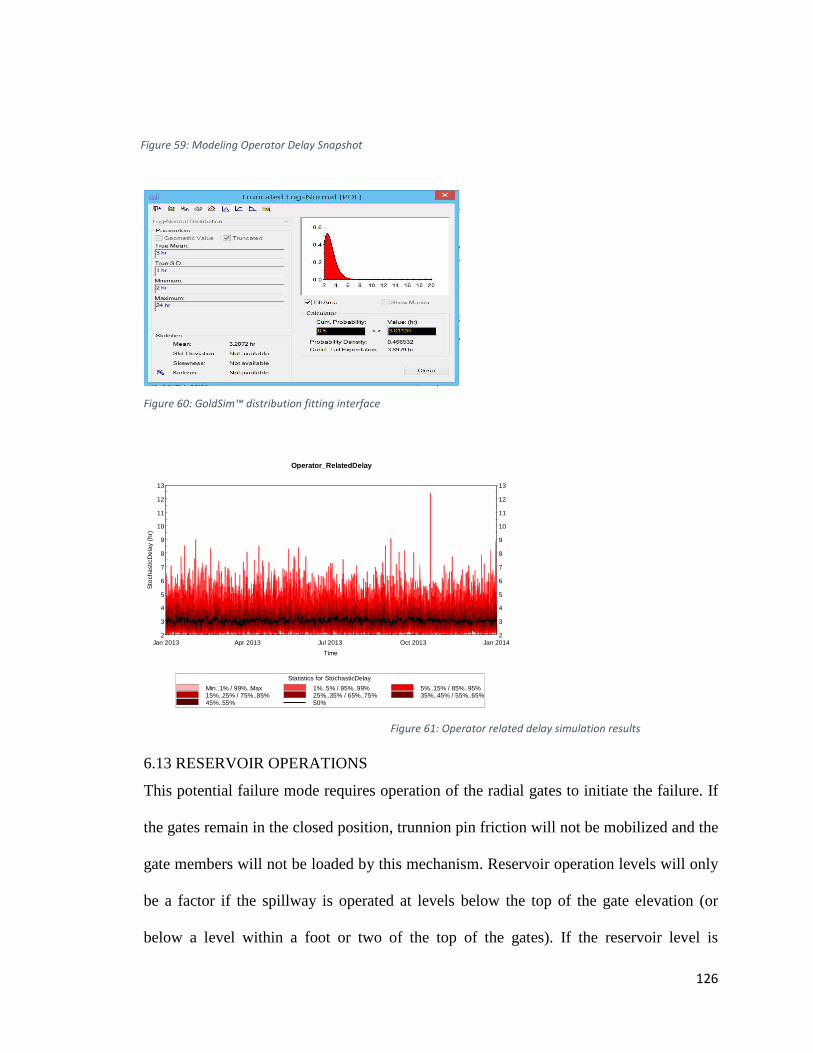
126
Figure 60: GoldSim™ distribution fitting interface
6.13 RESERVOIR OPERATIONS
This potential failure mode requires operation of the radial gates to initiate the failure. If
the gates remain in the closed position, trunnion pin friction will not be mobilized and the
gate members will not be loaded by this mechanism. Reservoir operation levels will only
be a factor if the spillway is operated at levels below the top of the gate elevation (or
below a level within a foot or two of the top of the gates). If the reservoir level is
2
3
4
5
6
7
8
9
10
11
12
13
Jan 2013 Apr 2013 Jul 2013 Oct 2013 Jan 2014
Sto
chas
ticD
elay
(hr
)
Time
2
3
4
5
6
7
8
9
10
11
12
13
Operator_RelatedDelay
Statistics for StochasticDelay
Min..1% / 99%..Max 1%..5% / 95%..99% 5%..15% / 85%..95%15%..25% / 75%..85% 25%..35% / 65%..75% 35%..45% / 55%..65%45%..55% 50%
Figure 59: Modeling Operator Delay Snapshot
Figure 61: Operator related delay simulation results
127
typically at or near the top of the gates on an annual basis when the gates are likely to be
operated or tested, this is a more hazardous situation than if the reservoir frequently does
not reach the top of the gates on an annual basis, or the gates are typically tested when the
reservoir is low. The likelihood of various reservoir levels at times when the gates will be
operated can typically be estimated from the historic reservoir exceedance curves.
6.14 ACCOUNTING FOR PERFORMANCE UNCERTAINTY
Typically, the reservoir elevation exceedance probabilities are taken directly from the
historical reservoir operations data, directly, which do not account for uncertainty.
Uncertainty in the failure probability and consequences are accounted for by entering the
estimates as distributions (as describe above) rather than single point values. A “Monte
Carlo” simulation is then run to display the uncertainty in the estimates, as described in
the section on Combining and Portraying Risks.
6.14.1 RELIABILITY OF SYSTEMS A structural system may have multiple components and failure modes. A structure is
considered safe or reliable if its capacity, C, exceeds the demand, D, placed on it:
C ≥ D or C − D ≥ 0 or ≥ 1 or "# $ 1
The reliability of a structure, ps, is the probability that the structure survives or performs
safely.
Hence probability of failure Pf, can be defined as
Pf =1- Ps
Equation 2
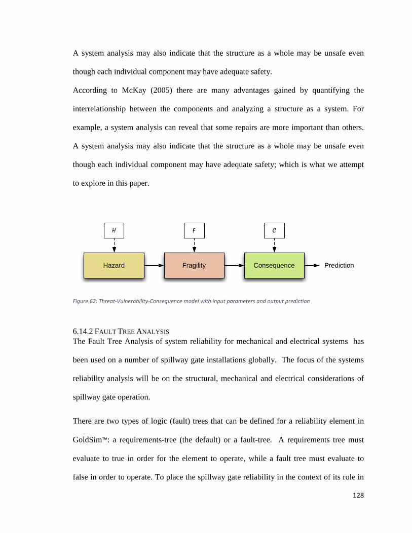
128
A system analysis may also indicate that the structure as a whole may be unsafe even
though each individual component may have adequate safety.
According to McKay (2005) there are many advantages gained by quantifying the
interrelationship between the components and analyzing a structure as a system. For
example, a system analysis can reveal that some repairs are more important than others.
A system analysis may also indicate that the structure as a whole may be unsafe even
though each individual component may have adequate safety; which is what we attempt
to explore in this paper.
Figure 62: Threat-Vulnerability-Consequence model with input parameters and output prediction
6.14.2 FAULT TREE ANALYSIS The Fault Tree Analysis of system reliability for mechanical and electrical systems has
been used on a number of spillway gate installations globally. The focus of the systems
reliability analysis will be on the structural, mechanical and electrical considerations of
spillway gate operation.
There are two types of logic (fault) trees that can be defined for a reliability element in
GoldSim™: a requirements-tree (the default) or a fault-tree. A requirements tree must
evaluate to true in order for the element to operate, while a fault tree must evaluate to
false in order to operate. To place the spillway gate reliability in the context of its role in
Hazard Fragility Consequence
H F C
Prediction
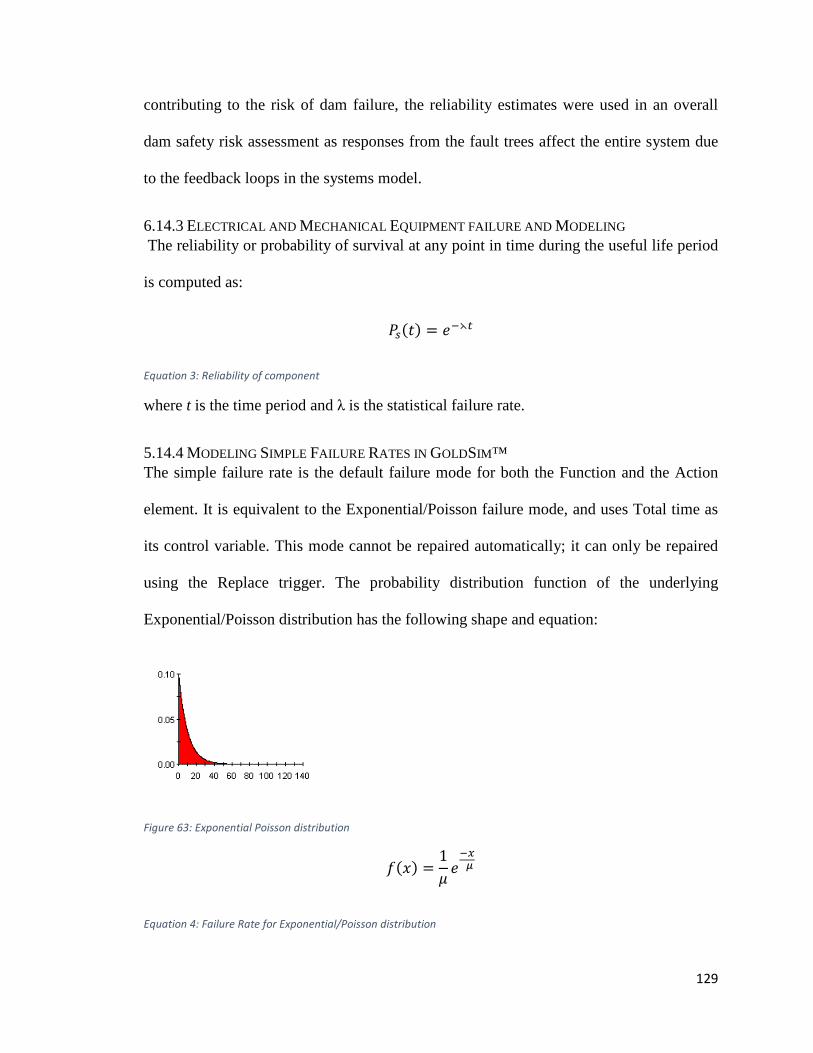
129
contributing to the risk of dam failure, the reliability estimates were used in an overall
dam safety risk assessment as responses from the fault trees affect the entire system due
to the feedback loops in the systems model.
6.14.3 ELECTRICAL AND MECHANICAL EQUIPMENT FAILURE AND MODELING The reliability or probability of survival at any point in time during the useful life period
is computed as:
&'�! � �()*
Equation 3: Reliability of component
where t is the time period and λ is the statistical failure rate.
5.14.4 MODELING SIMPLE FAILURE RATES IN GOLDSIM™ The simple failure rate is the default failure mode for both the Function and the Action
element. It is equivalent to the Exponential/Poisson failure mode, and uses Total time as
its control variable. This mode cannot be repaired automatically; it can only be repaired
using the Replace trigger. The probability distribution function of the underlying
Exponential/Poisson distribution has the following shape and equation:
Figure 63: Exponential Poisson distribution
��+! � 1, �
(- .
Equation 4: Failure Rate for Exponential/Poisson distribution
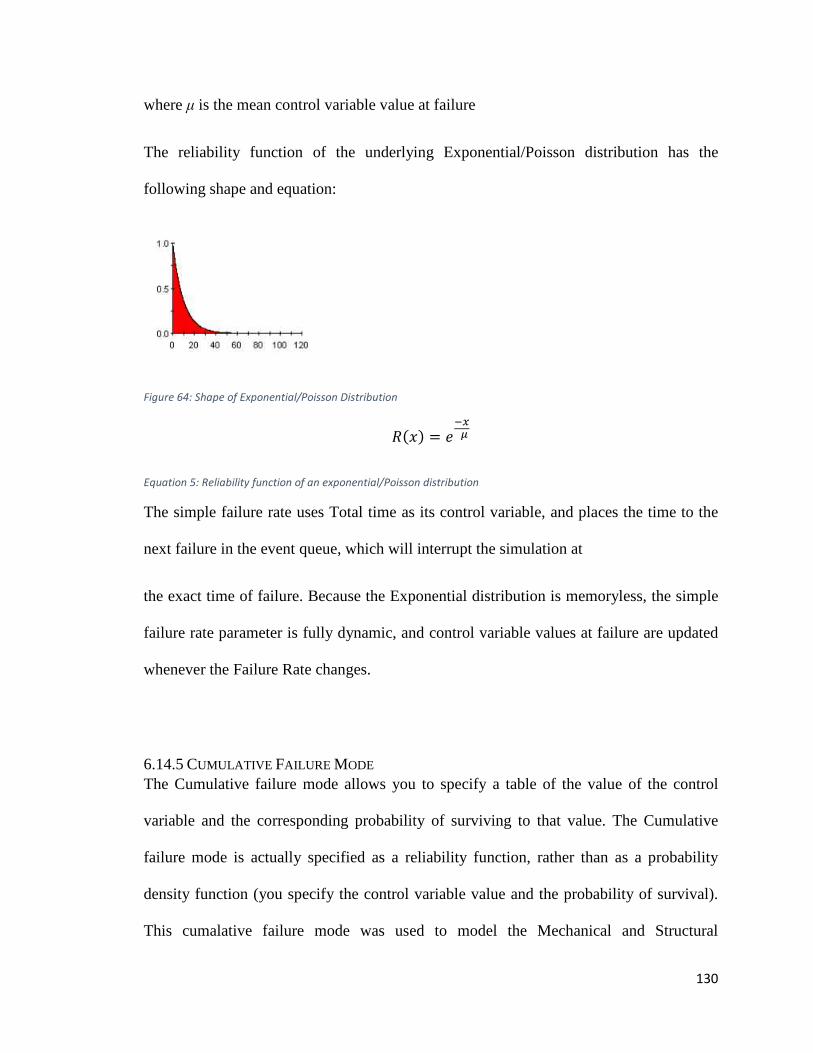
130
where µ is the mean control variable value at failure
The reliability function of the underlying Exponential/Poisson distribution has the
following shape and equation:
Figure 64: Shape of Exponential/Poisson Distribution
��+! � �(- .
Equation 5: Reliability function of an exponential/Poisson distribution
The simple failure rate uses Total time as its control variable, and places the time to the
next failure in the event queue, which will interrupt the simulation at
the exact time of failure. Because the Exponential distribution is memoryless, the simple
failure rate parameter is fully dynamic, and control variable values at failure are updated
whenever the Failure Rate changes.
6.14.5 CUMULATIVE FAILURE MODE The Cumulative failure mode allows you to specify a table of the value of the control
variable and the corresponding probability of surviving to that value. The Cumulative
failure mode is actually specified as a reliability function, rather than as a probability
density function (you specify the control variable value and the probability of survival).
This cumalative failure mode was used to model the Mechanical and Structural
131
component failure at LMR complex by using modified fragility curves from another dam
project the this paper had some time constraints which did not make it possible to wait for
the actual LMR comple fragility curves for the gates.
6.14.6 THE FRAGILITY CURVE In safety or risk assessment of dams, limit states or probability of failure serve as
yardsticks of system performance. The fragility curve is used to predict the probably of
dam failure, given the hydraulic hazard (Chase, 2012). The fragility curve is defined by
the cumulative distribution function (CDF) of the system response curve.
For example of a dam in which the overtopping limit state, i.e., FSovertopped≤ 1.0, is the
limit state resulting in failure of the dam.
The probability of failure, Pfailure, is given by the expression:
P0123456 � 7 &���8965*8::6; < 1.0 ? &��� �@ABBC
D:883!&�&��� � D:883!
Equation 6: Probability of failure for fragility curves
In which Pool is a vector of random variables describing the intensity of demand (e.g.
pool elevation, etc.) and other factors; P(Pool = D:883) is the hazard, considering channel
inflows and storm runoff from the watershed behind the dam, and is expressed in terms of
annual probability; and P(��8965*8::6;≤ 1.0 | Pool = D:883 ) is the conditional
probability of structural failure, given that Pool = D:883, Expressing the limit state
probability as in Equation 5 allows the overall risk to be deconstructed into its significant
contributors (Chase, 2012).
The fragility curve is defined by the cumulative distribution function (CDF) of the system
response curve. The CDF for both mechanical and structural failure can be observed in
figure 61 and figure 63 with the failure mode control variable (Height of water elevation

on Gates) on the X axis and the Cumulative
62 and 64 also show the hazard rating curves, that is; the probability of failure at a
specified level of the Failure mode control variable (FMCV).
Mechanical fragility
Figure 65: Cumulative Distribution curve for Mechanical Equipment
Figure 66: Fragility Curve for Mechanical Gate
Gates) on the X axis and the Cumulative Survival rate on the Y axis on t
also show the hazard rating curves, that is; the probability of failure at a
specified level of the Failure mode control variable (FMCV).
: Cumulative Distribution curve for Mechanical Equipment Survival
: Fragility Curve for Mechanical Gate Failure
132
on the Y axis. Fig
also show the hazard rating curves, that is; the probability of failure at a
Figure 68: Fragility Curve for Structural Gate Failure
6.14.7 ELECTRICAL FAILURE
The Failure Rate (also known as the hazard rate) represents the mean failure
dimensions of inverse time. Failure is assumed to be a Poisson process (which implies
that if the rate is constant, the time between events is exponentially distributed).
Fragility Curve for Structural Gate Failure
AILURE The Failure Rate (also known as the hazard rate) represents the mean failure
time. Failure is assumed to be a Poisson process (which implies
is constant, the time between events is exponentially distributed).
Figure 67: Cumulative Distributing curve for Structural gate Survival
133
Structu
ral
Failure
The Failure Rate (also known as the hazard rate) represents the mean failure rate, and has
time. Failure is assumed to be a Poisson process (which implies
is constant, the time between events is exponentially distributed). Failures
Figure 67: Cumulative Distributing curve for Structural gate Survival
134
modeled in this way are computed with respect to the time since the simulation started an
hence the time is the failure mode control valuable.
Electrical Reliability, specified as the electrical availability On Demand of the System
(including operator push button error and external and internal power failures) is
estimated at 0.017 faliures per day.
6.15 REPAIR TIME DISTRIBUTIONS USED FOR THE LMR
Gamma Distribution
For repairs (down time), the Gamma distribution is specified using a mean delay time
until repair (µ) and a standard deviation (σ). The Gamma distribution has the following
shape and equation:
��+! � E�E+!F(G�(H-
Γ�J!
Equation 7: Failure rate of a gamma distribution
Where J � .KLK ��� E � .
LK
Figure 69: Gamma Distribution
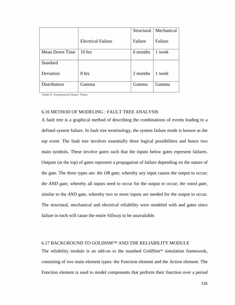
135
Electrical Failure
Structural
Failure
Mechanical
Failure
Mean Down Time 10 hrs 6 months 1 week
Standard
Deviation 8 hrs 2 months 1 week
Distribution Gamma Gamma Gamma
Table 9: Component Down Times
6.16 METHOD OF MODELING : FAULT TREE ANALYSIS
A fault tree is a graphical method of describing the combinations of events leading to a
defined system failure. In fault tree terminology, the system failure mode is known as the
top event. The fault tree involves essentially three logical possibilities and hence two
main symbols. These involve gates such that the inputs below gates represent failures.
Outputs (at the top) of gates represent a propagation of failure depending on the nature of
the gate. The three types are: the OR gate, whereby any input causes the output to occur;
the AND gate, whereby all inputs need to occur for the output to occur; the voted gate,
similar to the AND gate, whereby two or more inputs are needed for the output to occur.
The structural, mechanical and electrical reliability were modeled with and gates since
failure in each will cause the entire Sillway to be unavailable.
6.17 BACKGROUND TO GOLDSIM™ AND THE RELIABILITY MODULE
The reliability module is an add-on to the standard GoldSim™ simulation framework,
consisting of two main element types: the Function element and the Action element. The
Function element is used to model components that perform their function over a period
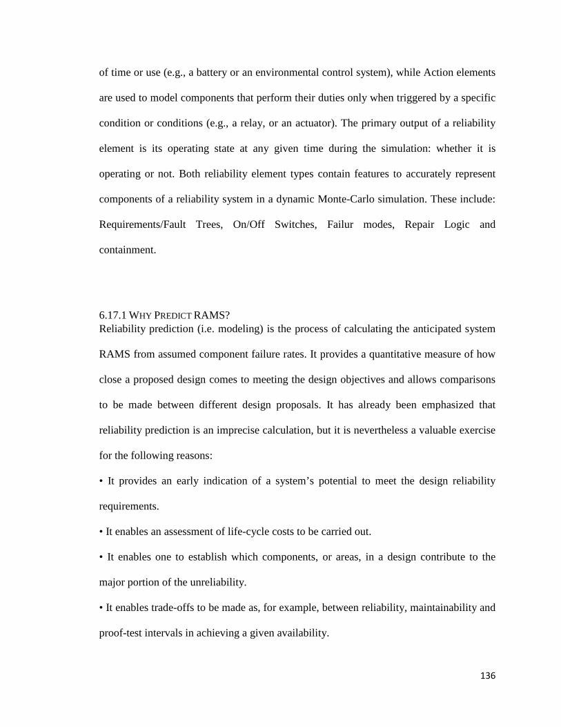
136
of time or use (e.g., a battery or an environmental control system), while Action elements
are used to model components that perform their duties only when triggered by a specific
condition or conditions (e.g., a relay, or an actuator). The primary output of a reliability
element is its operating state at any given time during the simulation: whether it is
operating or not. Both reliability element types contain features to accurately represent
components of a reliability system in a dynamic Monte-Carlo simulation. These include:
Requirements/Fault Trees, On/Off Switches, Failur modes, Repair Logic and
containment.
6.17.1 WHY PREDICT RAMS? Reliability prediction (i.e. modeling) is the process of calculating the anticipated system
RAMS from assumed component failure rates. It provides a quantitative measure of how
close a proposed design comes to meeting the design objectives and allows comparisons
to be made between different design proposals. It has already been emphasized that
reliability prediction is an imprecise calculation, but it is nevertheless a valuable exercise
for the following reasons:
• It provides an early indication of a system’s potential to meet the design reliability
requirements.
• It enables an assessment of life-cycle costs to be carried out.
• It enables one to establish which components, or areas, in a design contribute to the
major portion of the unreliability.
• It enables trade-offs to be made as, for example, between reliability, maintainability and
proof-test intervals in achieving a given availability.
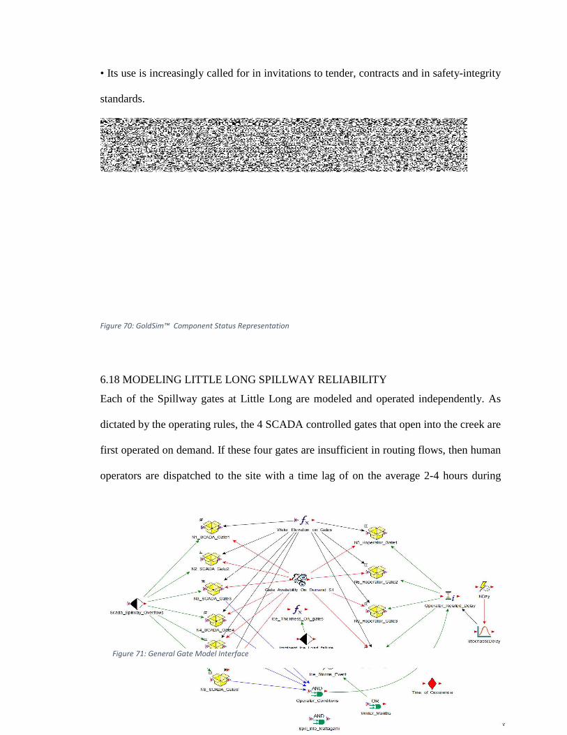
137
• Its use is increasingly called for in invitations to tender, contracts and in safety-integrity
standards.
Figure 70: GoldSim™ Component Status Representation
6.18 MODELING LITTLE LONG SPILLWAY RELIABILITY
Each of the Spillway gates at Little Long are modeled and operated independently. As
dictated by the operating rules, the 4 SCADA controlled gates that open into the creek are
first operated on demand. If these four gates are insufficient in routing flows, then human
operators are dispatched to the site with a time lag of on the average 2-4 hours during
Figure 71: General Gate Model Interface
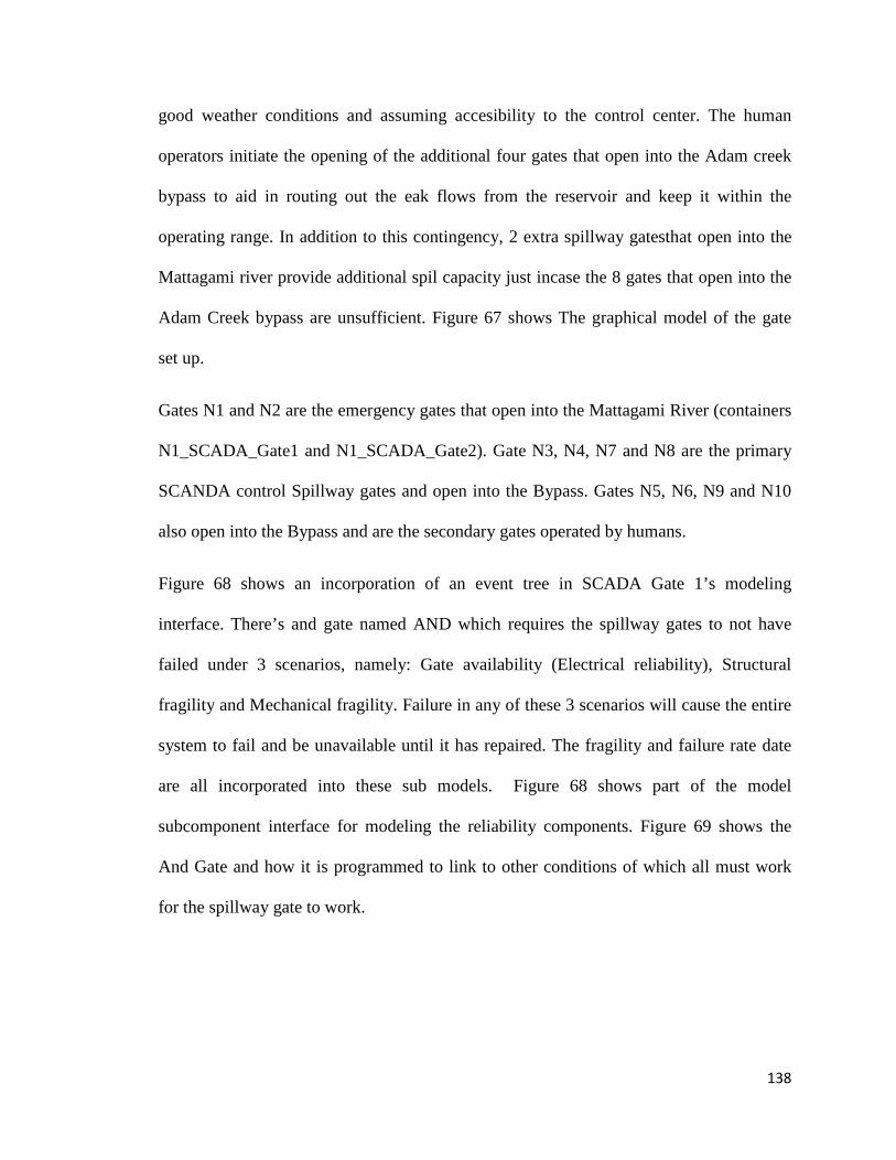
138
good weather conditions and assuming accesibility to the control center. The human
operators initiate the opening of the additional four gates that open into the Adam creek
bypass to aid in routing out the eak flows from the reservoir and keep it within the
operating range. In addition to this contingency, 2 extra spillway gatesthat open into the
Mattagami river provide additional spil capacity just incase the 8 gates that open into the
Adam Creek bypass are unsufficient. Figure 67 shows The graphical model of the gate
set up.
Gates N1 and N2 are the emergency gates that open into the Mattagami River (containers
N1_SCADA_Gate1 and N1_SCADA_Gate2). Gate N3, N4, N7 and N8 are the primary
SCANDA control Spillway gates and open into the Bypass. Gates N5, N6, N9 and N10
also open into the Bypass and are the secondary gates operated by humans.
Figure 68 shows an incorporation of an event tree in SCADA Gate 1’s modeling
interface. There’s and gate named AND which requires the spillway gates to not have
failed under 3 scenarios, namely: Gate availability (Electrical reliability), Structural
fragility and Mechanical fragility. Failure in any of these 3 scenarios will cause the entire
system to fail and be unavailable until it has repaired. The fragility and failure rate date
are all incorporated into these sub models. Figure 68 shows part of the model
subcomponent interface for modeling the reliability components. Figure 69 shows the
And Gate and how it is programmed to link to other conditions of which all must work
for the spillway gate to work.
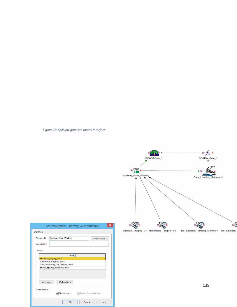
Figure 72: Spillway gate sub model Interface
Figure 72: Spillway gate sub model Interface
139
6.19 GATE OPERATIONS
Imminent Dam Failure during reservoir inflow floods (Overtopping Failure) is assumed
to occur when water reache
failure elevation; thus when the elevation exceeds the imminent dam failure elevation.
Figure 73: GoldSim™ And Properties Dialog
GATE OPERATIONS AND RESULTS ANALYSIS
Imminent Dam Failure during reservoir inflow floods (Overtopping Failure) is assumed
to occur when water reaches a stage specified the operating documents as imminent dam
failure elevation; thus when the elevation exceeds the imminent dam failure elevation.
Figure 74: GoldSim™ Reliability Function Properties
Interface
140
Imminent Dam Failure during reservoir inflow floods (Overtopping Failure) is assumed
s a stage specified the operating documents as imminent dam
failure elevation; thus when the elevation exceeds the imminent dam failure elevation.
74: GoldSim™ Reliability Function Properties

141
Figure 68 shows a snapshot of the one of the Spillway gates sub model interface. A high-
level model is useful in understanding some of the behavior patterns responsible for the
unavailability of a spill way gate on demand; which induces a high risk of system failure.
A simulation for a year from start of a calendar year to end of calendar year was run by
sampling a calendar years’ worth of inflow data from the historic time series and routing
it through the system. Figure 71 shows a plot of SCADA controlled Spills within a single
calendar year as a function of time. A graph of the upstream daily flow is also
superimposed on the plot to enable viewing the correlation between the upstream daily
flow and the SCADA controlled Spillway discharges (withdrawals). As expected, the two
are heavily correlated with the peak flows coinciding with the peak Spillway discharges
by the SCADA controlled gates. Each Spillway gate has a maximum capacity of 608.8
cubic meters; meaning the combined capacity of the four spillway gates is about 2400
cubic meters. During peak inflows we can see that the combined effect of the four gates
is around this capacity.
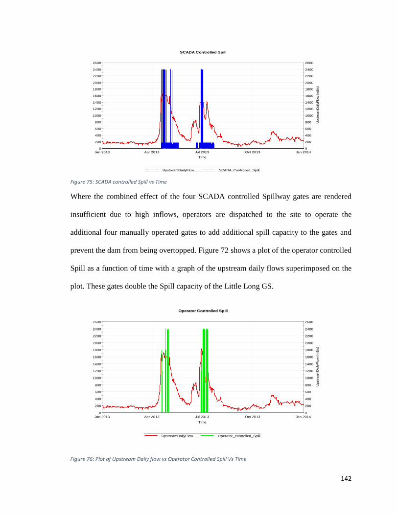
142
Where the combined effect of the four SCADA controlled Spillway gates are rendered
insufficient due to high inflows, operators are dispatched to the site to operate the
additional four manually operated gates to add additional spill capacity to the gates and
prevent the dam from being overtopped. Figure 72 shows a plot of the operator controlled
Spill as a function of time with a graph of the upstream daily flows superimposed on the
plot. These gates double the Spill capacity of the Little Long GS.
Figure 76: Plot of Upstream Daily flow vs Operator Controlled Spill Vs Time
0
200
400
600
800
1000
1200
1400
1600
1800
2000
2200
2400
2600
Jan 2013 Apr 2013 Jul 2013 Oct 2013 Jan 2014
Time
0
200
400
600
800
1000
1200
1400
1600
1800
2000
2200
2400
2600
Ups
trea
mD
aily
Flo
w (
m3/
s)
Operator Controlled Spill
UpstreamDailyFlow Operator_controlled_Spill
0
200
400
600
800
1000
1200
1400
1600
1800
2000
2200
2400
2600
Jan 2013 Apr 2013 Jul 2013 Oct 2013 Jan 2014
Time
0
200
400
600
800
1000
1200
1400
1600
1800
2000
2200
2400
2600
Ups
trea
mD
aily
Flo
w (m
3/s)
SCADA Controlled Spill
UpstreamDailyFlow SCADA_Controlled_Spill
Figure 75: SCADA controlled Spill vs Time
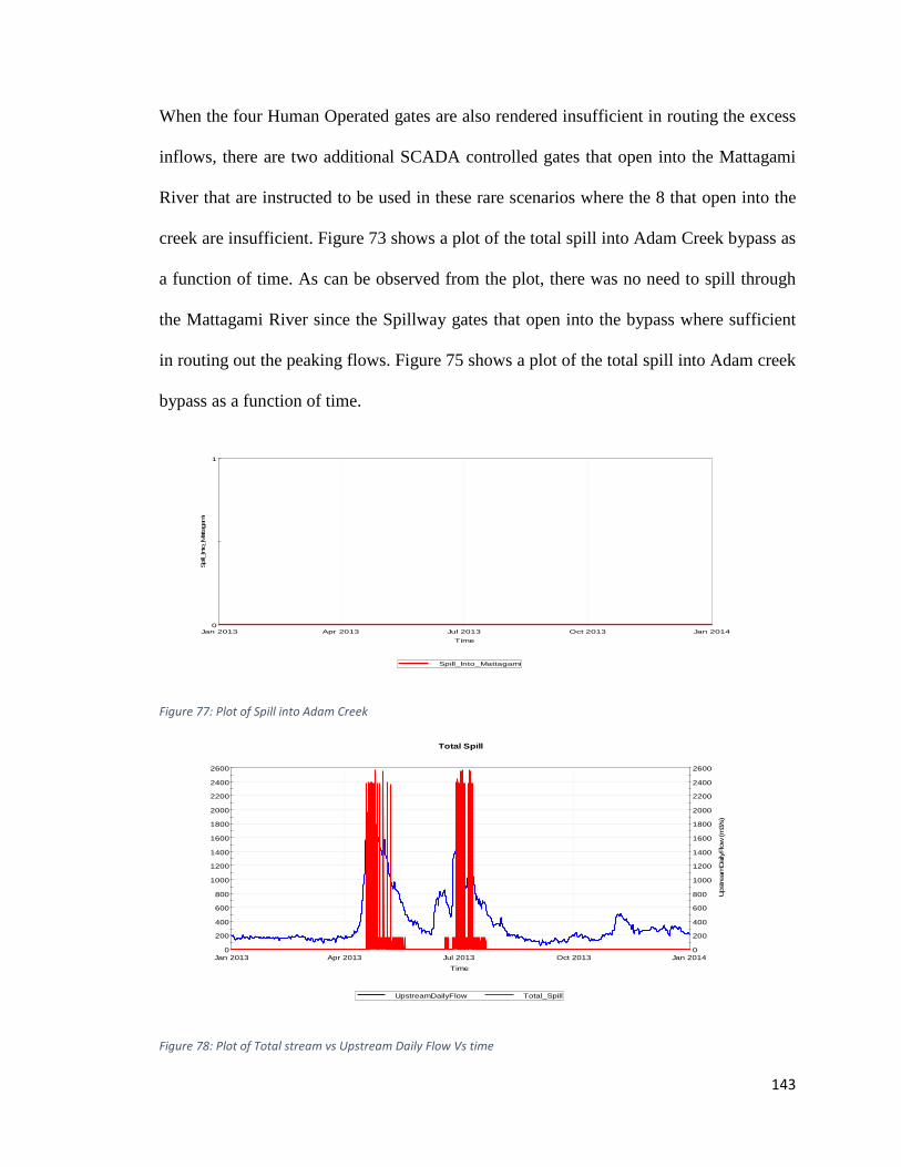
143
When the four Human Operated gates are also rendered insufficient in routing the excess
inflows, there are two additional SCADA controlled gates that open into the Mattagami
River that are instructed to be used in these rare scenarios where the 8 that open into the
creek are insufficient. Figure 73 shows a plot of the total spill into Adam Creek bypass as
a function of time. As can be observed from the plot, there was no need to spill through
the Mattagami River since the Spillway gates that open into the bypass where sufficient
in routing out the peaking flows. Figure 75 shows a plot of the total spill into Adam creek
bypass as a function of time.
Figure 77: Plot of Spill into Adam Creek
Figure 78: Plot of Total stream vs Upstream Daily Flow Vs time
0
1
Jan 2013 Apr 2013 Jul 2013 Oct 2013 Jan 2014
Spill_
lnto_Mattaga
mi
Time
Spill_lnto_Mattagami
0
200
400
600
800
1000
1200
1400
1600
1800
2000
2200
2400
2600
Jan 2013 Apr 2013 Jul 2013 Oct 2013 Jan 2014
Time
0
200
400
600
800
1000
1200
1400
1600
1800
2000
2200
2400
2600
Upst
ream
Daily
Flo
w (m
3/s
)
Total Spill
UpstreamDailyFlow Total_Spill
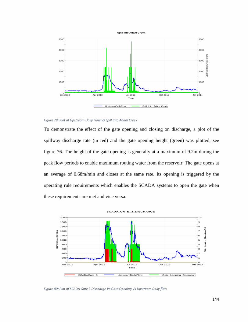
144
Figure 79: Plot of Upstream Daily Flow Vs Spill Into Adam Creek
To demonstrate the effect of the gate opening and closing on discharge, a plot of the
spillway discharge rate (in red) and the gate opening height (green) was plotted; see
figure 76. The height of the gate opening is generally at a maximum of 9.2m during the
peak flow periods to enable maximum routing water from the reservoir. The gate opens at
an average of 0.68m/min and closes at the same rate. Its opening is triggered by the
operating rule requirements which enables the SCADA systems to open the gate when
these requirements are met and vice versa.
Figure 80: Plot of SCADA Gate 3 Discharge Vs Gate Opening Vs Upstream Daily flow
0
1000
2000
3000
4000
5000
Jan 2013 Apr 2013 Jul 2013 Oct 2013 Jan 2014
Time
0
1000
2000
3000
4000
5000
Ups
trea
mD
aily
Flo
w (m
3/s)
Spill Into Adam Creek
UpstreamDailyFlow Spill_Into_Adam_Creek
0
200
400
600
800
1000
1200
1400
1600
1800
2000
Jan 2013 Apr 2013 Jul 2013 Oct 2013 Jan 2014
SCADAGate_3
(m3/s)
Time
0
1
2
3
4
5
6
7
8
9
10
Gate_L
ooping
_Ope
ratio
n (m
)
SCADA_GATE_3_DISCHARGE
SCADAGate_3 UpstreamDailyFlow Gate_Looping_Operation
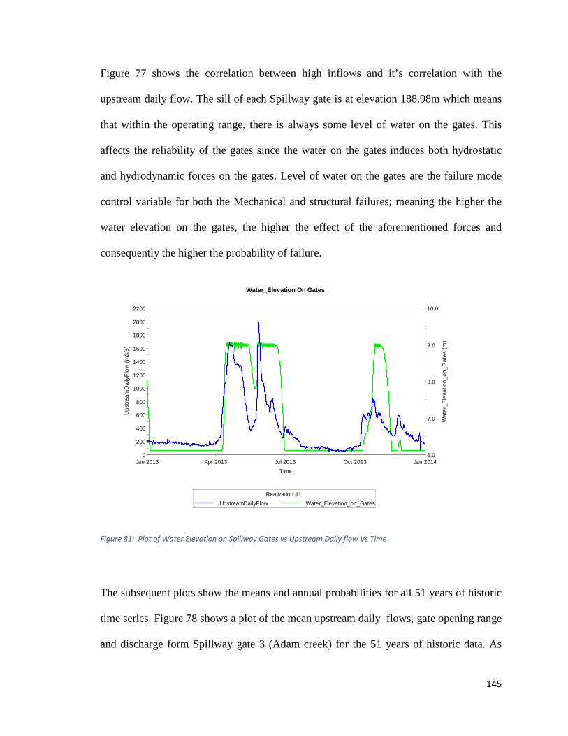
145
Figure 77 shows the correlation between high inflows and it’s correlation with the
upstream daily flow. The sill of each Spillway gate is at elevation 188.98m which means
that within the operating range, there is always some level of water on the gates. This
affects the reliability of the gates since the water on the gates induces both hydrostatic
and hydrodynamic forces on the gates. Level of water on the gates are the failure mode
control variable for both the Mechanical and structural failures; meaning the higher the
water elevation on the gates, the higher the effect of the aforementioned forces and
consequently the higher the probability of failure.
Figure 81: Plot of Water Elevation on Spillway Gates vs Upstream Daily flow Vs Time
The subsequent plots show the means and annual probabilities for all 51 years of historic
time series. Figure 78 shows a plot of the mean upstream daily flows, gate opening range
and discharge form Spillway gate 3 (Adam creek) for the 51 years of historic data. As
0
200
400
600
800
1000
1200
1400
1600
1800
2000
2200
Jan 2013 Apr 2013 Jul 2013 Oct 2013 Jan 2014
Ups
tre
amD
aily
Flo
w (
m3
/s)
Time
6.0
7.0
8.0
9.0
10.0
Wat
er_E
leva
tion_
on_
Gat
es
(m)
Water_Elevation On Gates
Realization #1
UpstreamDailyFlow Water_Elevation_on_Gates
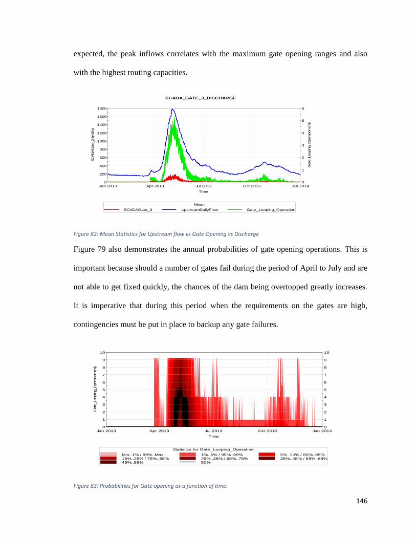
146
expected, the peak inflows correlates with the maximum gate opening ranges and also
with the highest routing capacities.
Figure 82: Mean Statistics for Upstream flow vs Gate Opening vs Discharge
Figure 79 also demonstrates the annual probabilities of gate opening operations. This is
important because should a number of gates fail during the period of April to July and are
not able to get fixed quickly, the chances of the dam being overtopped greatly increases.
It is imperative that during this period when the requirements on the gates are high,
contingencies must be put in place to backup any gate failures.
Figure 83: Probabilities for Gate opening as a function of time.
0
200
400
600
800
1000
1200
1400
1600
1800
Jan 2013 Apr 2013 Jul 2013 Oct 2013 Jan 2014
SC
AD
AG
ate_
3 (m
3/s)
Time
0
1
2
3
4
5
6
Gate
_Lo
opin
g_O
pera
tion
(m)
SCADA_GATE_3_DISCHARGE
Mean
SCADAGate_3 UpstreamDailyFlow Gate_Looping_Operation
0
1
2
3
4
5
6
7
8
9
10
Jan 2013 Apr 2013 Jul 2013 Oct 2013 Jan 2014
Gat
e_L
oopin
g_O
pera
tion (m
)
Time
0
1
2
3
4
5
6
7
8
9
10
Statistics for Gate_Looping_Operation
Min..1% / 99%..Max 1%..5% / 95%..99% 5%..15% / 85%..95%15%..25% / 75%..85% 25%..35% / 65%..75% 35%..45% / 55%..65%45%..55% 50%
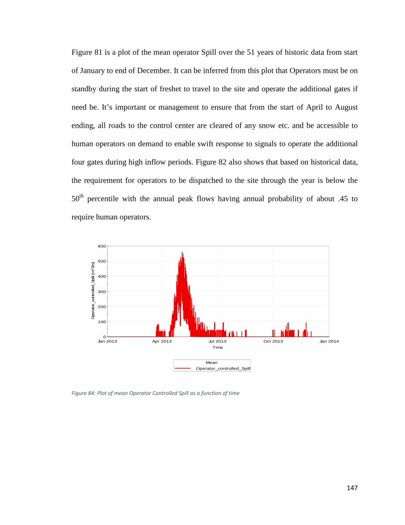
147
Figure 81 is a plot of the mean operator Spill over the 51 years of historic data from start
of January to end of December. It can be inferred from this plot that Operators must be on
standby during the start of freshet to travel to the site and operate the additional gates if
need be. It’s important or management to ensure that from the start of April to August
ending, all roads to the control center are cleared of any snow etc. and be accessible to
human operators on demand to enable swift response to signals to operate the additional
four gates during high inflow periods. Figure 82 also shows that based on historical data,
the requirement for operators to be dispatched to the site through the year is below the
50th percentile with the annual peak flows having annual probability of about .45 to
require human operators.
Figure 84: Plot of mean Operator Controlled Spill as a function of time
0
100
200
300
400
500
600
Jan 2013 Apr 2013 Jul 2013 Oct 2013 Jan 2014
Ope
rato
r_co
ntro
lled_
Spi
ll (m̂
3/s)
Time
Mean
Operator_controlled_Spill
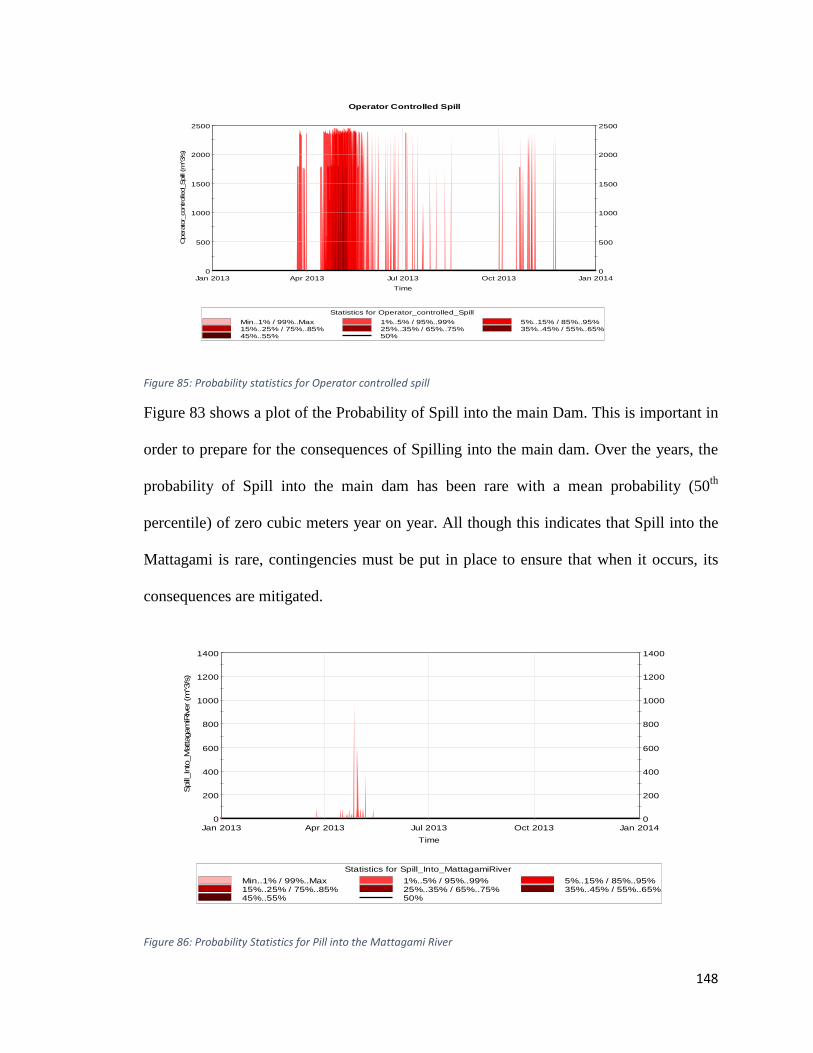
148
Figure 85: Probability statistics for Operator controlled spill
Figure 83 shows a plot of the Probability of Spill into the main Dam. This is important in
order to prepare for the consequences of Spilling into the main dam. Over the years, the
probability of Spill into the main dam has been rare with a mean probability (50th
percentile) of zero cubic meters year on year. All though this indicates that Spill into the
Mattagami is rare, contingencies must be put in place to ensure that when it occurs, its
consequences are mitigated.
Figure 86: Probability Statistics for Pill into the Mattagami River
0
500
1000
1500
2000
2500
Jan 2013 Apr 2013 Jul 2013 Oct 2013 Jan 2014
Ope
rato
r_co
ntro
lled_
Spi
ll (m̂
3/s)
Time
0
500
1000
1500
2000
2500
Operator Controlled Spill
Statistics for Operator_controlled_Spill
Min..1% / 99%..Max 1%..5% / 95%..99% 5%..15% / 85%..95%15%..25% / 75%..85% 25%..35% / 65%..75% 35%..45% / 55%..65%45%..55% 50%
0
200
400
600
800
1000
1200
1400
Jan 2013 Apr 2013 Jul 2013 Oct 2013 Jan 2014
Spi
ll_In
to_M
atta
gam
iRiver
(m̂
3/s)
Time
0
200
400
600
800
1000
1200
1400
Statistics for Spill_Into_MattagamiRiver
Min..1% / 99%..Max 1%..5% / 95%..99% 5%..15% / 85%..95%15%..25% / 75%..85% 25%..35% / 65%..75% 35%..45% / 55%..65%45%..55% 50%
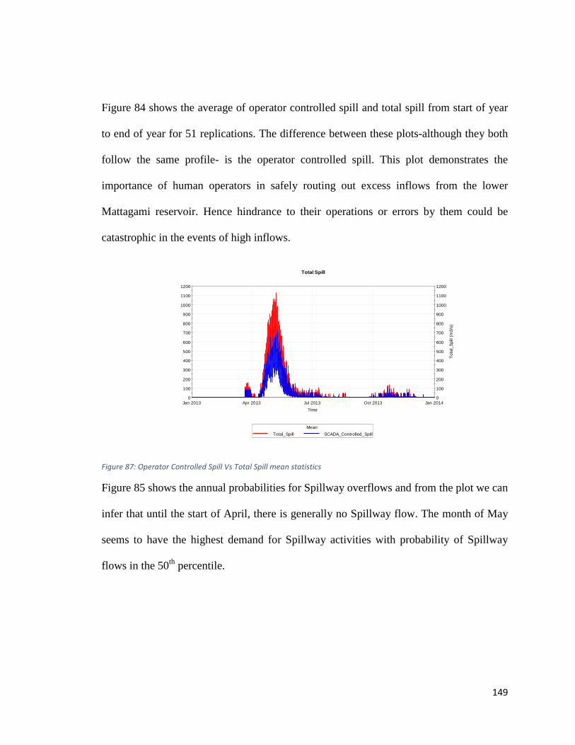
149
Figure 84 shows the average of operator controlled spill and total spill from start of year
to end of year for 51 replications. The difference between these plots-although they both
follow the same profile- is the operator controlled spill. This plot demonstrates the
importance of human operators in safely routing out excess inflows from the lower
Mattagami reservoir. Hence hindrance to their operations or errors by them could be
catastrophic in the events of high inflows.
Figure 87: Operator Controlled Spill Vs Total Spill mean statistics
Figure 85 shows the annual probabilities for Spillway overflows and from the plot we can
infer that until the start of April, there is generally no Spillway flow. The month of May
seems to have the highest demand for Spillway activities with probability of Spillway
flows in the 50th percentile.
0
100
200
300
400
500
600
700
800
900
1000
1100
1200
Jan 2013 Apr 2013 Jul 2013 Oct 2013 Jan 2014
Time
0
100
200
300
400
500
600
700
800
900
1000
1100
1200
Tot
al_
Sp
ill (
m3
/s)
Total Spill
Mean
Total_Spill SCADA_Controlled_Spill
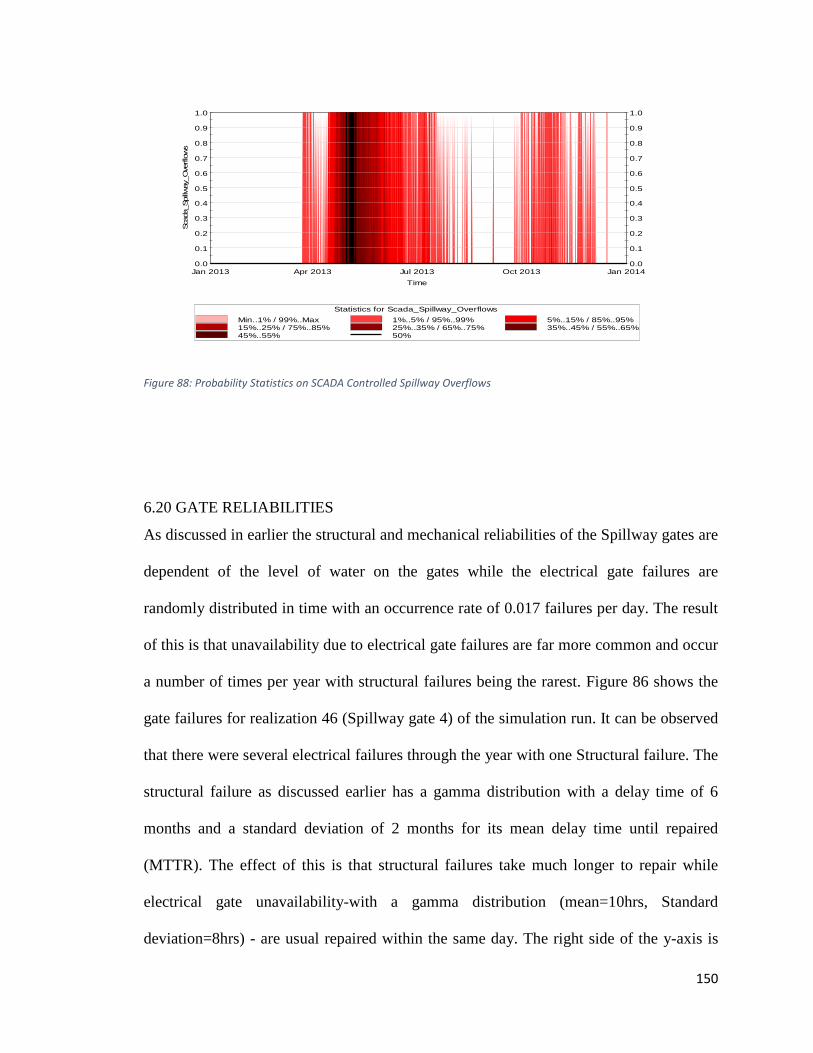
150
Figure 88: Probability Statistics on SCADA Controlled Spillway Overflows
6.20 GATE RELIABILITIES
As discussed in earlier the structural and mechanical reliabilities of the Spillway gates are
dependent of the level of water on the gates while the electrical gate failures are
randomly distributed in time with an occurrence rate of 0.017 failures per day. The result
of this is that unavailability due to electrical gate failures are far more common and occur
a number of times per year with structural failures being the rarest. Figure 86 shows the
gate failures for realization 46 (Spillway gate 4) of the simulation run. It can be observed
that there were several electrical failures through the year with one Structural failure. The
structural failure as discussed earlier has a gamma distribution with a delay time of 6
months and a standard deviation of 2 months for its mean delay time until repaired
(MTTR). The effect of this is that structural failures take much longer to repair while
electrical gate unavailability-with a gamma distribution (mean=10hrs, Standard
deviation=8hrs) - are usual repaired within the same day. The right side of the y-axis is
0.0
0.1
0.2
0.3
0.4
0.5
0.6
0.7
0.8
0.9
1.0
Jan 2013 Apr 2013 Jul 2013 Oct 2013 Jan 2014
Sca
da_S
pillw
ay_
Ove
rflo
ws
Time
0.0
0.1
0.2
0.3
0.4
0.5
0.6
0.7
0.8
0.9
1.0
Statistics for Scada_Spillway_Overflows
Min..1% / 99%..Max 1%..5% / 95%..99% 5%..15% / 85%..95%15%..25% / 75%..85% 25%..35% / 65%..75% 35%..45% / 55%..65%45%..55% 50%
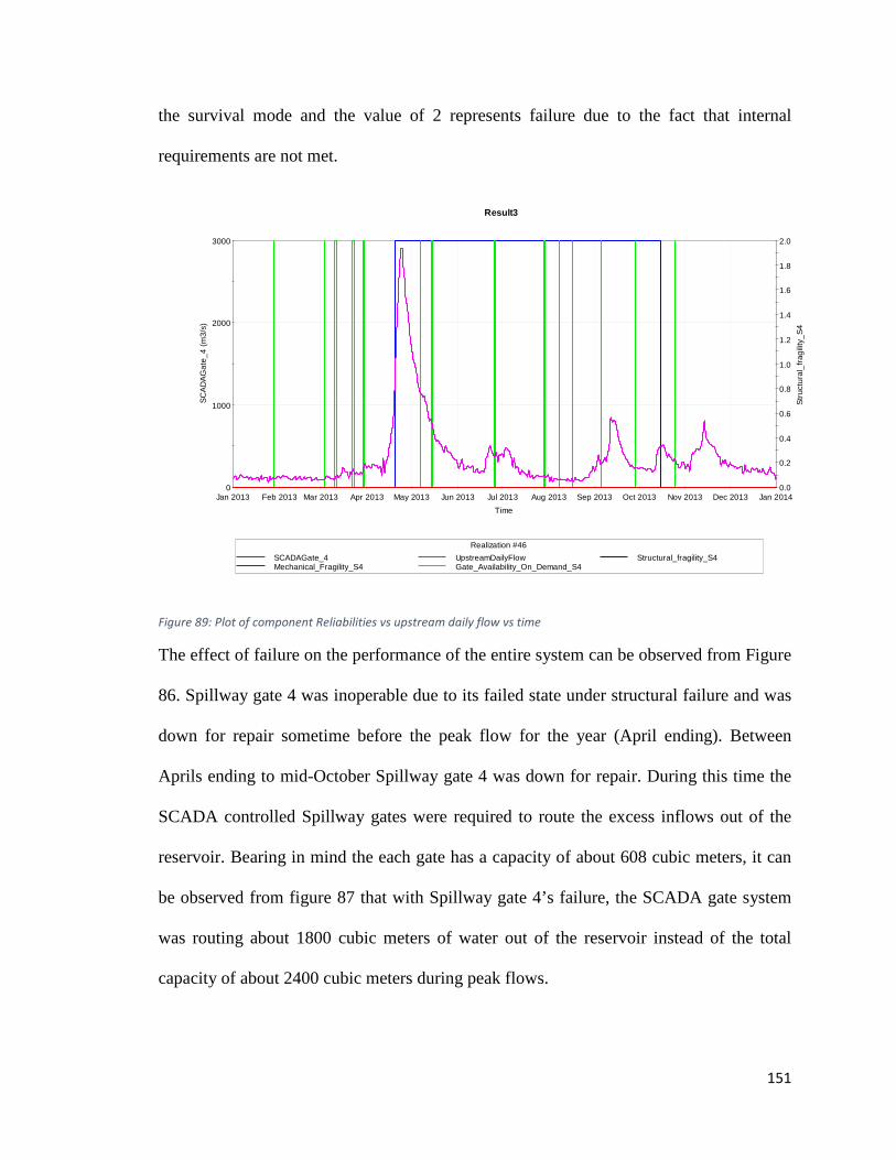
151
the survival mode and the value of 2 represents failure due to the fact that internal
requirements are not met.
Figure 89: Plot of component Reliabilities vs upstream daily flow vs time
The effect of failure on the performance of the entire system can be observed from Figure
86. Spillway gate 4 was inoperable due to its failed state under structural failure and was
down for repair sometime before the peak flow for the year (April ending). Between
Aprils ending to mid-October Spillway gate 4 was down for repair. During this time the
SCADA controlled Spillway gates were required to route the excess inflows out of the
reservoir. Bearing in mind the each gate has a capacity of about 608 cubic meters, it can
be observed from figure 87 that with Spillway gate 4’s failure, the SCADA gate system
was routing about 1800 cubic meters of water out of the reservoir instead of the total
capacity of about 2400 cubic meters during peak flows.
0
1000
2000
3000
Jan 2013 Feb 2013 Mar 2013 Apr 2013 May 2013 Jun 2013 Jul 2013 Aug 2013 Sep 2013 Oct 2013 Nov 2013 Dec 2013 Jan 2014
SC
AD
AG
ate_
4 (m
3/s
)
Time
0.0
0.2
0.4
0.6
0.8
1.0
1.2
1.4
1.6
1.8
2.0
Str
uctu
ral_
frag
ility
_S4
Result3
Realization #46
SCADAGate_4 UpstreamDailyFlow Structural_fragility_S4Mechanical_Fragility_S4 Gate_Availability_On_Demand_S4
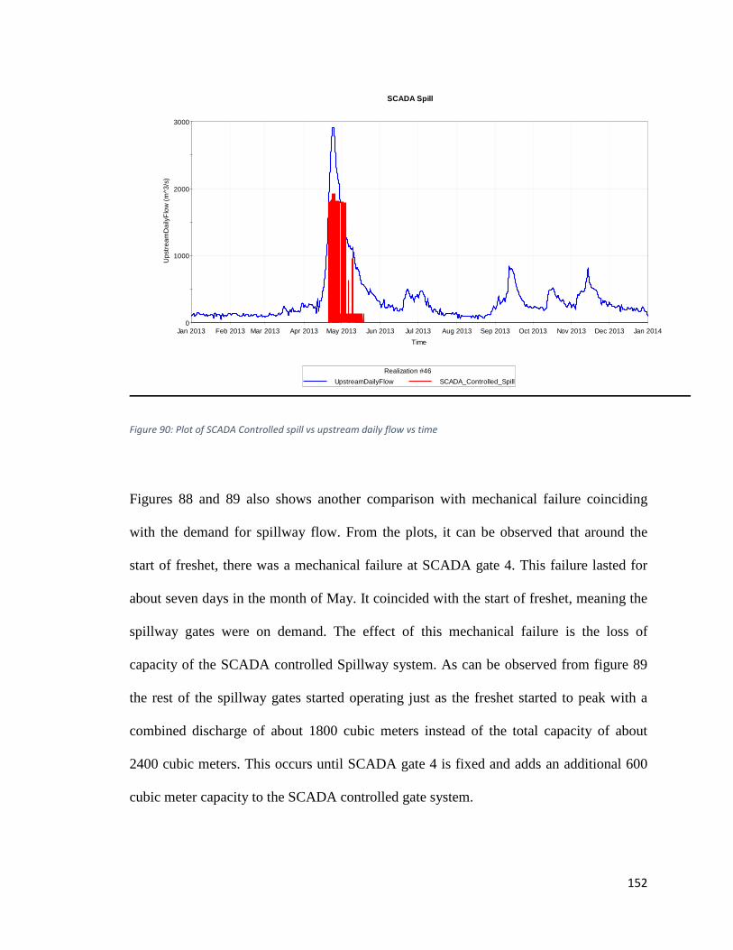
152
Figure 90: Plot of SCADA Controlled spill vs upstream daily flow vs time
Figures 88 and 89 also shows another comparison with mechanical failure coinciding
with the demand for spillway flow. From the plots, it can be observed that around the
start of freshet, there was a mechanical failure at SCADA gate 4. This failure lasted for
about seven days in the month of May. It coincided with the start of freshet, meaning the
spillway gates were on demand. The effect of this mechanical failure is the loss of
capacity of the SCADA controlled Spillway system. As can be observed from figure 89
the rest of the spillway gates started operating just as the freshet started to peak with a
combined discharge of about 1800 cubic meters instead of the total capacity of about
2400 cubic meters. This occurs until SCADA gate 4 is fixed and adds an additional 600
cubic meter capacity to the SCADA controlled gate system.
0
1000
2000
3000
Jan 2013 Feb 2013 Mar 2013 Apr 2013 May 2013 Jun 2013 Jul 2013 Aug 2013 Sep 2013 Oct 2013 Nov 2013 Dec 2013 Jan 2014
Ups
trea
mD
aily
Flo
w (
m^3
/s)
Time
SCADA Spill
Realization #46
UpstreamDailyFlow SCADA_Controlled_Spill
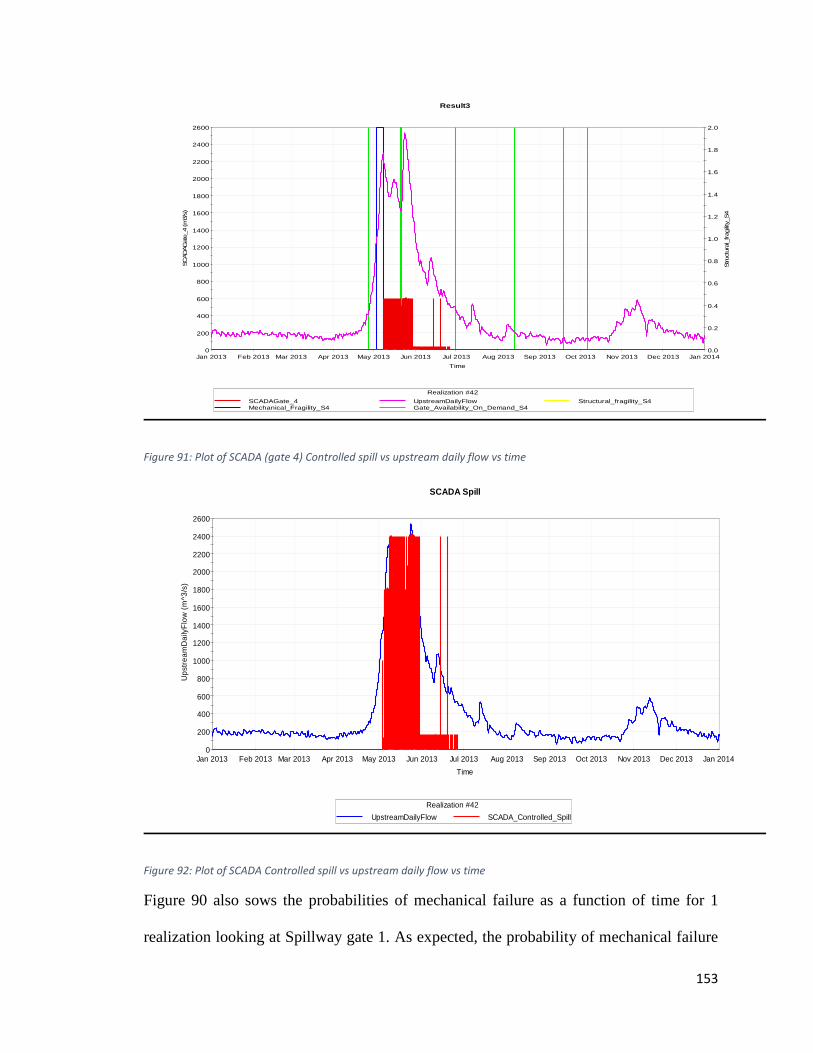
153
Figure 91: Plot of SCADA (gate 4) Controlled spill vs upstream daily flow vs time
Figure 92: Plot of SCADA Controlled spill vs upstream daily flow vs time
Figure 90 also sows the probabilities of mechanical failure as a function of time for 1
realization looking at Spillway gate 1. As expected, the probability of mechanical failure
0
200
400
600
800
1000
1200
1400
1600
1800
2000
2200
2400
2600
Jan 2013 Feb 2013 Mar 2013 Apr 2013 May 2013 Jun 2013 Jul 2013 Aug 2013 Sep 2013 Oct 2013 Nov 2013 Dec 2013 Jan 2014
SC
AD
AG
ate_4
(m
3/s)
Time
0.0
0.2
0.4
0.6
0.8
1.0
1.2
1.4
1.6
1.8
2.0
Struct
ura
l_frag
ility
_S4
Result3
Realization #42
SCADAGate_4 UpstreamDailyFlow Structural_fragility_S4Mechanical_Fragility_S4 Gate_Availability_On_Demand_S4
0
200
400
600
800
1000
1200
1400
1600
1800
2000
2200
2400
2600
Jan 2013 Feb 2013 Mar 2013 Apr 2013 May 2013 Jun 2013 Jul 2013 Aug 2013 Sep 2013 Oct 2013 Nov 2013 Dec 2013 Jan 2014
Ups
trea
mD
aily
Flo
w (
m^3
/s)
Time
SCADA Spill
Realization #42
UpstreamDailyFlow SCADA_Controlled_Spill
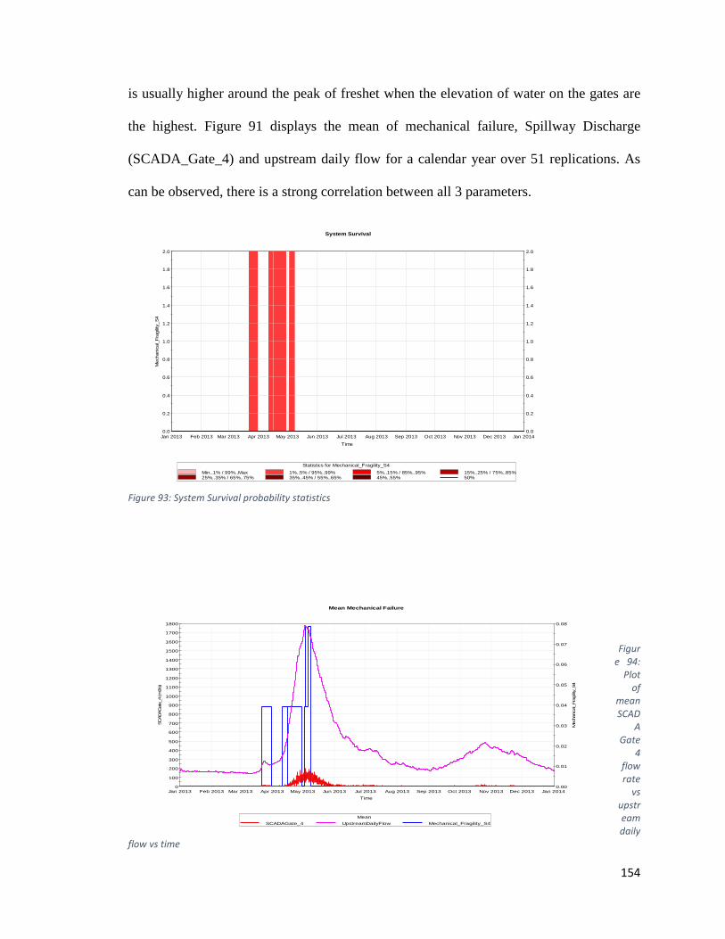
154
is usually higher around the peak of freshet when the elevation of water on the gates are
the highest. Figure 91 displays the mean of mechanical failure, Spillway Discharge
(SCADA_Gate_4) and upstream daily flow for a calendar year over 51 replications. As
can be observed, there is a strong correlation between all 3 parameters.
Figur
e 94:
Plot
of
mean
SCAD
A
Gate
4
flow
rate
vs
upstr
eam
daily
flow vs time
0.0
0.2
0.4
0.6
0.8
1.0
1.2
1.4
1.6
1.8
2.0
Jan 2013 Feb 2013 Mar 2013 Apr 2013 May 2013 Jun 2013 Jul 2013 Aug 2013 Sep 2013 Oct 2013 Nov 2013 Dec 2013 Jan 2014
Mech
anic
al_F
ragility
_S4
Time
0.0
0.2
0.4
0.6
0.8
1.0
1.2
1.4
1.6
1.8
2.0
System Survival
Statistics for Mechanical_Fragility_S4
Min..1% / 99%..Max 1%..5% / 95%..99% 5%..15% / 85%..95% 15%..25% / 75%..85%25%..35% / 65%..75% 35%..45% / 55%..65% 45%..55% 50%
0
100
200
300
400
500
600
700
800
900
1000
1100
1200
1300
1400
1500
1600
1700
1800
Jan 2013 Feb 2013 Mar 2013 Apr 2013 May 2013 Jun 2013 Jul 2013 Aug 2013 Sep 2013 Oct 2013 Nov 2013 Dec 2013 Jan 2014
SCADAG
ate_
4 (m
3/s)
Time
0.00
0.01
0.02
0.03
0.04
0.05
0.06
0.07
0.08
Mec
hani
cal_
Fra
gility_
S4
Mean Mechanical Failure
Mean
SCADAGate_4 UpstreamDailyFlow Mechanical_Fragility_S4
Figure 93: System Survival probability statistics
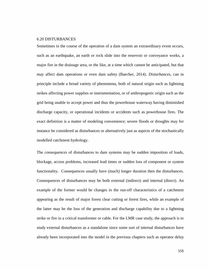
155
6.20 DISTURBANCES
Sometimes in the course of the operation of a dam system an extraordinary event occurs,
such as an earthquake, an earth or rock slide into the reservoir or conveyance works, a
major fire in the drainage area, or the like, at a time which cannot be anticipated, but that
may affect dam operations or even dam safety (Baecher, 2014). Disturbances, can in
principle include a broad variety of phenomena, both of natural origin such as lightning
strikes affecting power supplies or instrumentation, or of anthropogenic origin such as the
grid being unable to accept power and thus the powerhouse waterway having diminished
discharge capacity, or operational incidents or accidents such as powerhouse fires. The
exact definition is a matter of modeling convenience; severe floods or droughts may for
instance be considered as disturbances or alternatively just as aspects of the stochastically
modelled catchment hydrology.
The consequences of disturbances to dam systems may be sudden imposition of loads,
blockage, access problems, increased lead times or sudden loss of component or system
functionality. Consequences usually have (much) longer duration then the disturbances.
Consequences of disturbances may be both external (indirect) and internal (direct). An
example of the former would be changes in the run-off characteristics of a catchment
appearing as the result of major forest clear cutting or forest fires, while an example of
the latter may be the loss of the generation and discharge capability due to a lightning
strike or fire in a critical transformer or cable. For the LMR case study, the approach is to
study external disturbances as a standalone since some sort of internal disturbances have
already been incorporated into the model in the previous chapters such as operator delay
156
and power outages (grid availability on demand). The external disturbances that have
been considered are discussed in the next section.
6.20.1 EXTERNAL DISTURBANCES
When a disturbance occurs, for example an earthquake or a landslide into the reservoir, it
may cause damages to parts of the flow-control system, or it may trigger others
disturbances or consequences that in turn cause damage to the dam system. It may
simultaneously damage more than one component of the system, as for example, seismic
ground shaking might damage mechanical equipment in one or more spillway gates while
at the same time damaging the concrete conveyance carrying outflow from the gates. The
combinations of damages can exaggerate consequences by limiting redundancies in the
way the flow-control system operates.
An important factor in analysing disturbances is their causal interactions. For example,
both earthquakes and reservoir slides could be individually modelled as disturbances
occuring randomly in time with some frequency and severity. However, a reservoir slide
might also be caused by an earthquake, and thus not be “random” at all, except in the
sense that it is triggered by another natural hazard which is considered random.
The inter-arrival time between occurrences of the same or different types may itself be-
come a concern. For example, in traditional dam safety evaluations the joint occurrence
of an earthquake and an extreme hydrological event is ignored, because the two events
are logically independent and each of low probability, so their joint probability of
occurrence within a small period of time is vanishingly small. In practice, on the other
hand, should an earthquake occur and cause damage to the flow-control system which

157
cannot be repaired within an impending flood season, a subsequent large but not extreme
hydrological event may be uncontrollable due to the pre-existing spillway damage.
There are lots of external disturbances that can possible affect dam operations but two
main disturbances will be analysed and modelled for the LMR system case; namely
Debris and Ice. Consideration of other disturbances including the two aforementioned are
discussed in the next section.
6.20.2 POTENTIAL ENVIRONMENTAL CONDITIONS LIKELY EFFECTS ON THE LMR
Table 3 identifies the potential conditions in the environment that may affect the LMR
and its principal component(s) as adapted from the OPG proposal for the power
expansion project for LMR. Potential conditions arise from the physical environment
(i.e., natural hazards). The physical environment encompasses natural physical
phenomena on land, in bodies of water and in the atmosphere. The conditions included in
Table 7.2-1 are based on experience and potential conditions that have or could occur in
the LMR Complex. Each natural hazard and potential environmental condition, is
described in subsection 7.2.2.
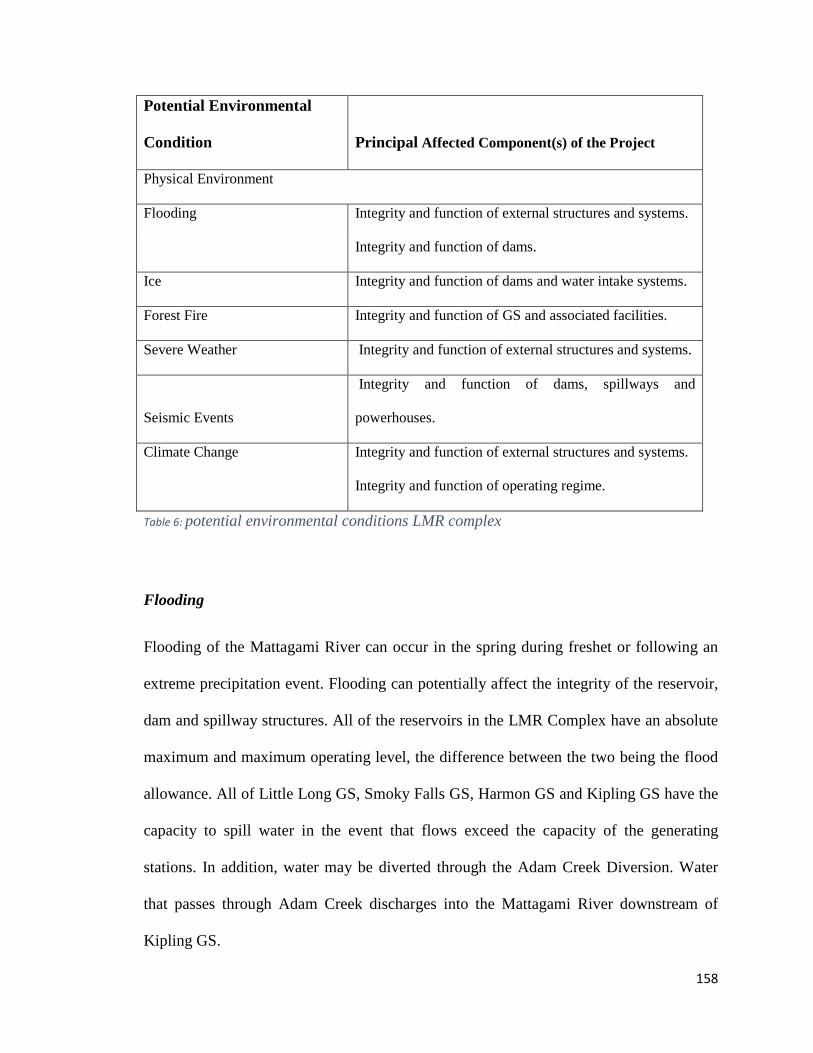
158
Potential Environmental
Condition Principal Affected Component(s) of the Project
Physical Environment
Flooding Integrity and function of external structures and systems.
Integrity and function of dams.
Ice Integrity and function of dams and water intake systems.
Forest Fire Integrity and function of GS and associated facilities.
Severe Weather Integrity and function of external structures and systems.
Seismic Events
Integrity and function of dams, spillways and
powerhouses.
Climate Change Integrity and function of external structures and systems.
Integrity and function of operating regime.
Table 6: potential environmental conditions LMR complex
Flooding
Flooding of the Mattagami River can occur in the spring during freshet or following an
extreme precipitation event. Flooding can potentially affect the integrity of the reservoir,
dam and spillway structures. All of the reservoirs in the LMR Complex have an absolute
maximum and maximum operating level, the difference between the two being the flood
allowance. All of Little Long GS, Smoky Falls GS, Harmon GS and Kipling GS have the
capacity to spill water in the event that flows exceed the capacity of the generating
stations. In addition, water may be diverted through the Adam Creek Diversion. Water
that passes through Adam Creek discharges into the Mattagami River downstream of
Kipling GS.
159
The effect of flooding and the probability of flooding causing dam failure is depending
on several parameters among which some have already been looked at in the previous
chapter.
Ice
The Mattagami River develops ice in the reservoirs beginning in November/December
with break-up typically occurring sometime in April. During the break-up of ice, jams
may form and have been reported downstream of Kipling GS. Even though the ice jam
occurs downstream of the stations, it may affect the tailwater levels at Kipling GS. The
formation of ice on the trash racks and gates is considered a routine maintenance issue
that is dealt with through bi-weekly inspections conducted by the OPG traveling operator
and maintenance crews. It is expected that continued maintenance will prevent ice issues
associated with station operation.
Forest Fires
The LMR Complex is surrounded by forest that may be impacted by fire. On a continual
basis, Natural Resources Canada evaluates a number of factors that estimate the potential
ease of a fire starting and spreading, how potentially difficult a fire would be to control as
well as the potential impacts of the fire to rate forest fire danger in an area (NRCAN
2007). The LMR complex has a moderate rating fire rating indicating that potential fires
are expected to be gentle surface fires that would be easily contained by ground crews
with pumps and hand tools.

160
Seismic Events
The Regional Study Area is located within the Northeastern Ontario seismic zone, which
is known to have a very low level of seismic activity (Earthquakes Canada, 2008a);
meaning that the probability of experiencing strong earthquake shaking is low. The
design of the each of Little Long GS, Smoky Falls GS, Harmon GS and Kipling GS
included the design of the dam, powerhouses and spillway structures using MNR
standards and in recognition of the Ontario Building Code. These structures were
designed to withstand the effects of a design basis seismic event. No further measures are
required to supplement the existing design and mitigation features in place to resist
seismic events. The potential for seismic events requires no further consideration as no
effect on the LMR complex is likely given the design considerations (Ontario Power
Generation Inc., 2009).
6.20.3 MODELING THE INHERENT DISTURBANCES Disturbances are generally modelled as a probability of occurrence of the hazard, an
identification of the assets that could be damaged, the vulnerability of those assets (i.e.,
the conditional probability of damage given the hazard occurs), and an assessment of the
economic and other consequences(Baecher, 2014).
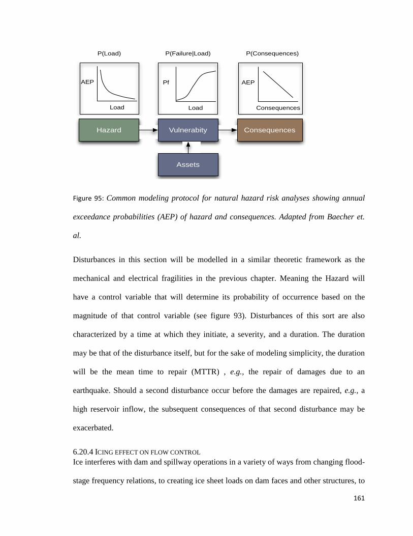
161
Figure 95: Common modeling protocol for natural hazard risk analyses showing annual
exceedance probabilities (AEP) of hazard and consequences. Adapted from Baecher et.
al.
Disturbances in this section will be modelled in a similar theoretic framework as the
mechanical and electrical fragilities in the previous chapter. Meaning the Hazard will
have a control variable that will determine its probability of occurrence based on the
magnitude of that control variable (see figure 93). Disturbances of this sort are also
characterized by a time at which they initiate, a severity, and a duration. The duration
may be that of the disturbance itself, but for the sake of modeling simplicity, the duration
will be the mean time to repair (MTTR) , e.g., the repair of damages due to an
earthquake. Should a second disturbance occur before the damages are repaired, e.g., a
high reservoir inflow, the subsequent consequences of that second disturbance may be
exacerbated.
6.20.4 ICING EFFECT ON FLOW CONTROL Ice interferes with dam and spillway operations in a variety of ways from changing flood-
stage frequency relations, to creating ice sheet loads on dam faces and other structures, to
Hazard Vulnerabity Consequences
Assets
Load
AEP
Load
Pf
Consequences
AEP
P(Load) P(Failure|Load) P(Consequences)
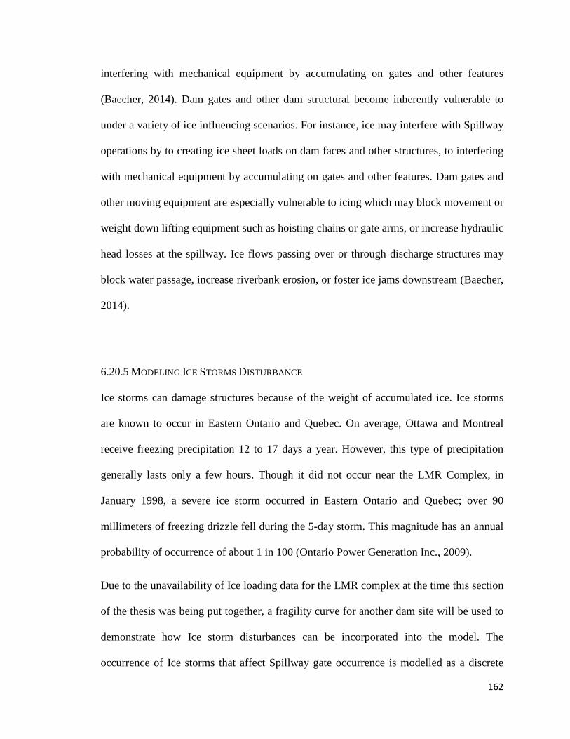
162
interfering with mechanical equipment by accumulating on gates and other features
(Baecher, 2014). Dam gates and other dam structural become inherently vulnerable to
under a variety of ice influencing scenarios. For instance, ice may interfere with Spillway
operations by to creating ice sheet loads on dam faces and other structures, to interfering
with mechanical equipment by accumulating on gates and other features. Dam gates and
other moving equipment are especially vulnerable to icing which may block movement or
weight down lifting equipment such as hoisting chains or gate arms, or increase hydraulic
head losses at the spillway. Ice flows passing over or through discharge structures may
block water passage, increase riverbank erosion, or foster ice jams downstream (Baecher,
2014).
6.20.5 MODELING ICE STORMS DISTURBANCE
Ice storms can damage structures because of the weight of accumulated ice. Ice storms
are known to occur in Eastern Ontario and Quebec. On average, Ottawa and Montreal
receive freezing precipitation 12 to 17 days a year. However, this type of precipitation
generally lasts only a few hours. Though it did not occur near the LMR Complex, in
January 1998, a severe ice storm occurred in Eastern Ontario and Quebec; over 90
millimeters of freezing drizzle fell during the 5-day storm. This magnitude has an annual
probability of occurrence of about 1 in 100 (Ontario Power Generation Inc., 2009).
Due to the unavailability of Ice loading data for the LMR complex at the time this section
of the thesis was being put together, a fragility curve for another dam site will be used to
demonstrate how Ice storm disturbances can be incorporated into the model. The
occurrence of Ice storms that affect Spillway gate occurrence is modelled as a discrete
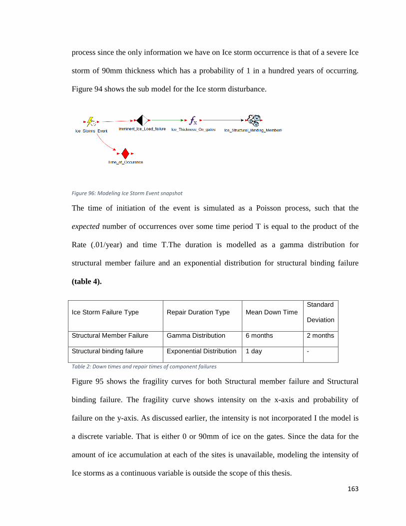
163
process since the only information we have on Ice storm occurrence is that of a severe Ice
storm of 90mm thickness which has a probability of 1 in a hundred years of occurring.
Figure 94 shows the sub model for the Ice storm disturbance.
Figure 96: Modeling Ice Storm Event snapshot
The time of initiation of the event is simulated as a Poisson process, such that the
expected number of occurrences over some time period T is equal to the product of the
Rate (.01/year) and time T.The duration is modelled as a gamma distribution for
structural member failure and an exponential distribution for structural binding failure
(table 4).
Ice Storm Failure Type Repair Duration Type Mean Down Time Standard
Deviation
Structural Member Failure Gamma Distribution 6 months 2 months
Structural binding failure Exponential Distribution 1 day -
Table 2: Down times and repair times of component failures
Figure 95 shows the fragility curves for both Structural member failure and Structural
binding failure. The fragility curve shows intensity on the x-axis and probability of
failure on the y-axis. As discussed earlier, the intensity is not incorporated I the model is
a discrete variable. That is either 0 or 90mm of ice on the gates. Since the data for the
amount of ice accumulation at each of the sites is unavailable, modeling the intensity of
Ice storms as a continuous variable is outside the scope of this thesis.
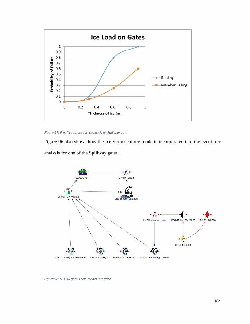
164
Figure 97: Fragility curves for Ice Loads on Spillway gate
Figure 96 also shows how the Ice Storm Failure mode is incorporated into the event tree
analysis for one of the Spillway gates.
Figure 98: SCADA gate 1 Sub model Interface
0
0.1
0.2
0.3
0.4
0.5
0.6
0.7
0.8
0.9
1
0 0.2 0.4 0.6 0.8 1
Pro
ba
bil
ity
of
Fa
ilu
re
Thickness of ice (m)
Ice Load on Gates
Binding
Member Failing
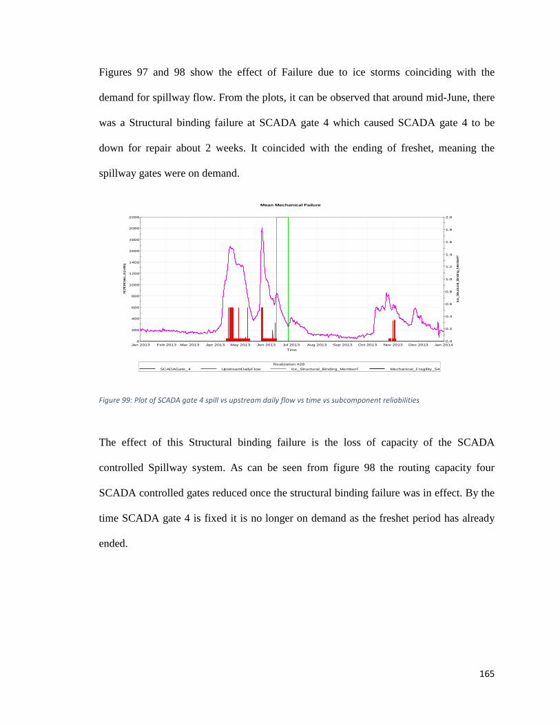
165
Figures 97 and 98 show the effect of Failure due to ice storms coinciding with the
demand for spillway flow. From the plots, it can be observed that around mid-June, there
was a Structural binding failure at SCADA gate 4 which caused SCADA gate 4 to be
down for repair about 2 weeks. It coincided with the ending of freshet, meaning the
spillway gates were on demand.
Figure 99: Plot of SCADA gate 4 spill vs upstream daily flow vs time vs subcomponent reliabilities
The effect of this Structural binding failure is the loss of capacity of the SCADA
controlled Spillway system. As can be seen from figure 98 the routing capacity four
SCADA controlled gates reduced once the structural binding failure was in effect. By the
time SCADA gate 4 is fixed it is no longer on demand as the freshet period has already
ended.
0
200
400
600
800
1000
1200
1400
1600
1800
2000
2200
Jan 2013 Feb 2013 Mar 2013 Apr 2013 May 2013 Jun 2013 Jul 2013 Aug 2013 Sep 2013 Oct 2013 Nov 2013 Dec 2013 Jan 2014
SCADAGat
e_4
(m3/
s)
Time
0.0
0.2
0.4
0.6
0.8
1.0
1.2
1.4
1.6
1.8
2.0
Ice_
Struc
tura
l_Binding
_Mem
berF
Mean Mechanical Failure
Realization #28
SCADAGate_4 UpstreamDailyFlow Ice_Structural_Binding_MemberF Mechanical_Fragility_S4
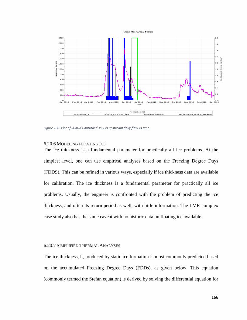
166
Figure 100: Plot of SCADA Controlled spill vs upstream daily flow vs time
6.20.6 MODELING FLOATING ICE
The ice thickness is a fundamental parameter for practically all ice problems. At the
simplest level, one can use empirical analyses based on the Freezing Degree Days
(FDDS). This can be refined in various ways, especially if ice thickness data are available
for calibration. The ice thickness is a fundamental parameter for practically all ice
problems. Usually, the engineer is confronted with the problem of predicting the ice
thickness, and often its return period as well, with little information. The LMR complex
case study also has the same caveat with no historic data on floating ice available.
6.20.7 SIMPLIFIED THERMAL ANALYSES
The ice thickness, h, produced by static ice formation is most commonly predicted based
on the accumulated Freezing Degree Days (FDDs), as given below. This equation
(commonly termed the Stefan equation) is derived by solving the differential equation for
0
200
400
600
800
1000
1200
1400
1600
1800
2000
2200
2400
Jan 2013 Feb 2013 Mar 2013 Apr 2013 May 2013 Jun 2013 Jul 2013 Aug 2013 Sep 2013 Oct 2013 Nov 2013 Dec 2013 Jan 2014
SCADAGate
_4 (m
3/s)
Time
0.0
0.2
0.4
0.6
0.8
1.0
1.2
1.4
1.6
1.8
2.0
Ice_
Structur
al_B
inding
_Mem
berF
Mean Mechanical Failure
Realization #28
SCADAGate_4 SCADA_Controlled_Spill UpstreamDailyFlow Ice_Structural_Binding_MemberF
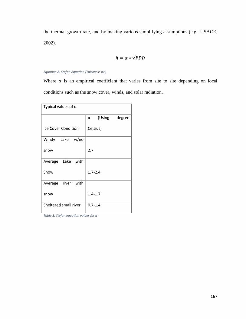
167
the thermal growth rate, and by making various simplifying assumptions (e.g., USACE,
2002).
� � M N √���
Equation 8: Stefan Equation (Thickness ice)
Where M is an empirical coefficient that varies from site to site depending on local
conditions such as the snow cover, winds, and solar radiation.
Typical values of α
Ice Cover Condition
α (Using degree
Celsius)
Windy Lake w/no
snow 2.7
Average Lake with
Snow 1.7-2.4
Average river with
snow 1.4-1.7
Sheltered small river 0.7-1.4
Table 3: Stefan equation values for α
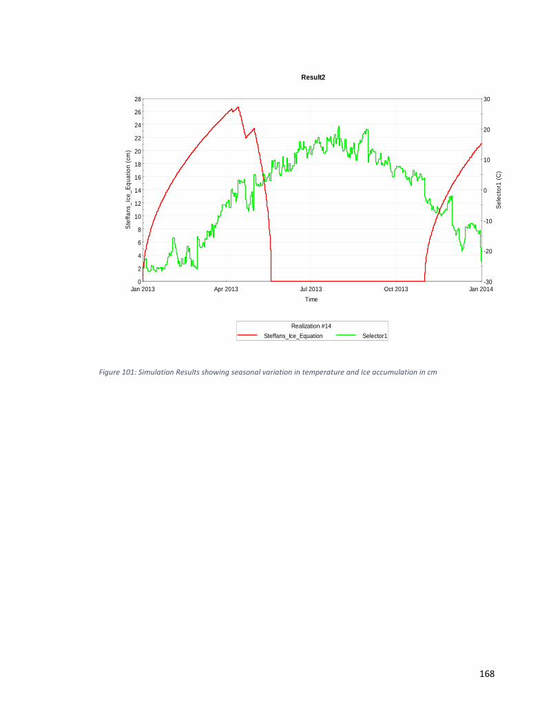
168
Figure 101: Simulation Results showing seasonal variation in temperature and Ice accumulation in cm
0
2
4
6
8
10
12
14
16
18
20
22
24
26
28
Jan 2013 Apr 2013 Jul 2013 Oct 2013 Jan 2014
Ste
ffans
_Ice
_Equ
atio
n (c
m)
Time
-30
-20
-10
0
10
20
30
Sel
ecto
r1 (
C)
Result2
Realization #14
Steffans_Ice_Equation Selector1
169
7.0 SUMMARY AND CONCLUSION
7.1 SUMMARY
This thesis advances on the developments made in the QRA field for engineering
reliability risk analyses. The lower Mattagami River Project was used as a case study to
demonstrate how far the development and application of systems reliability models has
come. The analysis approach is an outgrowth of a four-year effort by a joint-industry
consortium of hydropower operators to improve dam safety. In this thesis, the Systems
Reliability modeling concept is augmented with a Monte Carlo based simulation
framework to analyze the LMR case study and generate vital analytical outputs used to
analyze time-dependent risks, assist engineers and managers in safety/performance
related decision-making, create and test risk mitigation actions and policies, and monitor
the system for states of increasing risk. The practicality and usefulness of the Systems-
based Reliability model creation and analysis methodology was demonstrated using
OPG’s Lower Mattagami Basin cascade of four dams. The problem facing the project
was to conceptualize a systems engineering model for the operation of the dams,
spillways, and other components; then to employ the model through stochastic simulation
to investigate protocols for the safe operation of the spillway and flow control system.
Details of the modeling, analysis, and results for safe operation of the cascade are
presented in thesis.
170
7.2 CONCLUSION
The methodology and techniques presented in this thesis provide the foundation for
Simulation based Systems approach to dynamic Risk/Reliability model building and
analysis. This approach falls under the Quantitative risk assessment (QRA) methodology
and provides both a logical framework and a systematic procedure for organizing and
applying scientific and engineering knowledge to improve decision making in engineered
systems. Systems engineering and systems thinking represents a new dimension in risk
analysis for dam safety and has built on the advancements made using contemporary
methodologies such as event trees and fault tree analysis. The systems framework further
enhances the QRA field by providing a concept with more powerful tools and techniques
to holistically model and analyze time-dependent risks in complex systems. The
contemporary methods clamp different aspects of dam performance into separate failure
modes, and treat these failure modes separately(Baecher, 2014). The history of dam
safety suggests that accidents and failures occur in more complex ways, mostly due to
systems and human interactions, and need to be addressed in that way. The systems
approach addresses these flaws from first generation/contemporary approach. It does so
by approaching dams as engineered systems, and dam operations as an integral part of
safety (Baecher, 2014) . Modeling these systems quantitatively is a more complex
challenge than first generation analysis had been, and the task of verification and
validation of the tools to support the systems approach is presented in this thesis. The
thesis demonstrates how these new tools-via a readily available commercial software-can
be used perform an overall risk and reliability analysis of Dam systems.

171
The concept of model integration is essential to all systems modeling. As demonstrated in
this paper, accidents and failures occur not just because hazard loads are too high and
dam components are fragile, but through the interactions of physical systems, sensor and
SCADA systems, operating policies, human factors, and other aspects of dams. Fusing
models of different subsystems using the contemporary approach is difficult and
mathematically complex. Models of physical systems differ fundamentally from models
of sensor and SCADA system or from models of human operator actions or operational
rules(Baecher, 2014). The systems being modelled are complex and exhibit non-linear
behavior, from interacting components, often involving sub-systems that are themselves
complex. Data mining the outputs of the simulation runs enables us to also identify and
examine the build-up of conditions leading to accidents or failures, the time it takes for
some failure modes to progress from initiation to completion, the structure and nature of
dependency among failure modes and the nature of interactions among failure
mechanisms.
In conclusion modeling engineered systems via stochastic simulation using a systems
approach is very promising. In that, it affords us the platform to incorporate into the
model feedback of operating procedures and human reliability in systems function and
the ability to fuse models across different technological and human systems. Operational
procedures and human decision intervention strongly affect system operations, accidents,
and failures. These have not usually been accounted for in dam safety risk analysis and
the proposed systems simulation approach in this thesis does a good job of accounting for
systems interactions and feedback loops that are generally unaccounted for in the
contemporary methods.
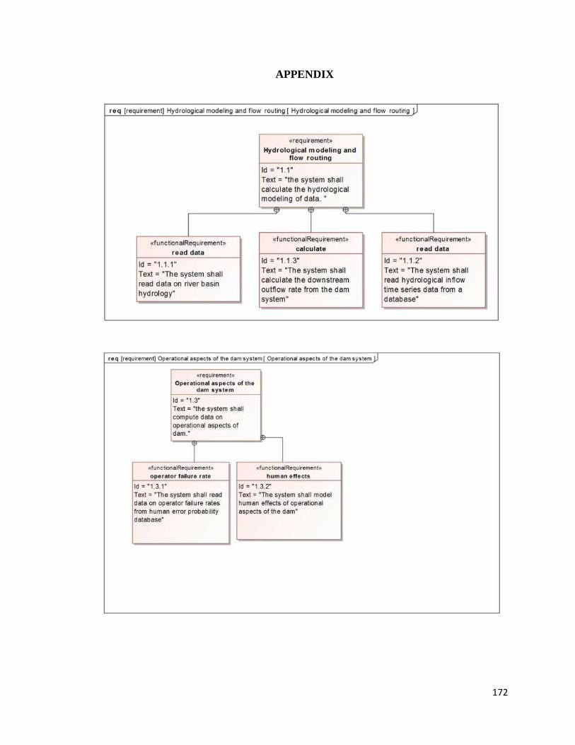
172
APPENDIX
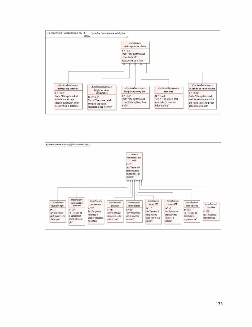
173
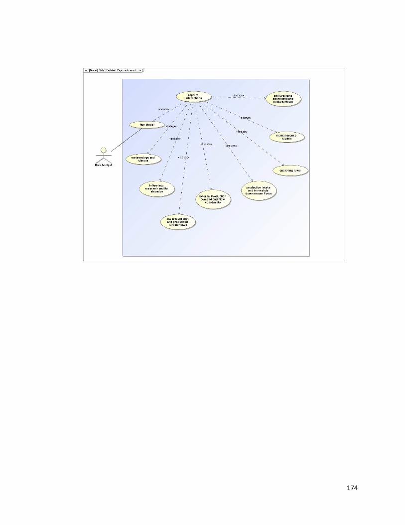
174

175
REFERENCES
Baecher, G. (2014). Second Generation Risk Analysis in Dam Safety. Forthcoming.
Thomas Telford.
Baecher, & Hartford. (2004). Risk and Uncertainty in Dam Safety. Thomas Telford.
Chase, Sr, M. E. (2012). Fragility Analysis of a Concrete Gravity Dam Embedded in
Rock and Its System Response Curve Computed by the Analytical Program
GDLAD_Foundation (Research No. ERDC TR-12-4). USACE.
Kossiakoff. (2011). Systems engineering: principles and practice. Hoboken, NJ: Wiley-
Interscience.
Leveson. (2011). Systems Thinking applied to Safety. MIT.
Maté, J. (2005). Requirements ENgineering for Socio-technical Systems. v: Information
Science Plublishing.
National Aeronautics and Space Administration NASA. (2007). Systems Engineering
Handbook Headquarters. Washington, D.C.
Ontario Power Generation Inc., M. C. F. N. (2009). LOWER MATTAGAMI RIVER
HYDROELECTRIC COMPLEX PROJECT. OPG.
Paul C. Rizzo Associates, Inc., W. B., P.E. (2013). DAM SAFETY PERFORMANCE
MONITORING AND DATA MANAGEMENT – BEST PRACTICES (CEATI No.
T082700-0210).
Regan. (2010). DAMS AS SYSTEMS — A HOLISTIC APPROACH TO DAM
SAFETY.

176