Embed Size (px)
Citation preview

-81-
Intervention of the Bank of Japan in Foreign ExchangeMarket and Its Effects on Volatility of Returns
Xinhong Lu t
Abstract
In this article, we perform several tests to determine whether the intervention of the Bank of Japan has an
asymmetric effect through GARCH type models. Furthermore, we use realized volatility calculated by high-
frequency exchange rate data to check the adequacy of the estimated volatility from GARCH type models.
Key Words : Intervention; Realized volatility; GARCH type models; High-frequency exchange rate data
JEL Classification : C20; E58; F31
1 IntroductionOne of the main roles of the central bank of any country is to stabilize its exchange rate. As is often
observed the exchange rate is volatile randomly over time and the central bank often intervenes to mitigate
the volatility. However, the effect of the intervention by the central bank seems so vague and inconclusive
that many researchers in economics and econometrics have been investigating its effectiveness for long
time. Chang and Taylor (1998) and Dominguez (1998) have introduced intervention variables as
explanatory variables into the mean and volatility equations in the ARCH model proposed by Bollerslev
(1986) to investigate the effects of intervention. Ito (2002) has found that the intervention of the Bank of
Japan (abbreviated as BOJ hereinafter) was effective in the late 1990s and the first few years of the 2000s
(from June 21, 1995 to March 31, 2003). Watanabe and Harada (2006) identify new evidence on the effects
of the BOJ' s intervention on the yen/dollar exchange rate volatility based on the component GARCH
model. In empirical studies it is often pointed out that the shocks to the financial market do not generate
equal responses. For stock markets, negative shocks have been found to generate a larger response than
positive shocks of equal magnitude. This empirical phenomenon is often referred to as asymmetric volatility
in the literature (see Engle and Ng, 1993; Zakoian, 1994). This phenomenon has been attributed to the
leverage effect for stock markets. For exchange rates, asymmetry has also been documented with no
apparent economic reason. Yet, ARCH models that allow asymmetric responses have been successfully
fitted to exchange rate data (see Hsieh, 1989; Byres and Peel, 1995; Kam, 1995; Hu et al, 1997; Tse and
Tsui, 1997; Kim, 1998, 1999; Lu, 2007). McKenzie (2002) attributes the presence of asymmetric responses
in exchange rate volatility to the intervention activity of the central bank, which suggests that intervention
might do more harm than good in volatile markets.
In this article, we perform several tests to determine whether the intervention of Bank of Japan has an
t Research Bureau, the People' s Bank of China, Building 2, No.32, Chengfang Street, Xicheng District, Beijing 100-800, China.
E-mail: [email protected]. Fax: +86-10-6601-6464, Tel: +86-10-66 19-5848.

-82-
asymmetric effect through GARCH type models. For this purpose we will take two approaches: First, to
determine whether there is any asymmetric effect on the exchange rate volatility, we analyze GJR,
EGARCH and APGARCH models, which can reflect asymmetry of the volatility under the constant mean
equation. In addition, we introduce the dummy variable D, , which takes 1 when the intervention takes
place and 0 elsewhere, in the variance equations in keeping the mean equation constant in GARCH type
models. The significant estimate of the coefficient of D, suggests that the intervention has an effect on the
exchange rate volatility. We call the first approach as 'variance equation approach'. Second, to determine
whether the intervention has an effect on the mean equation of the exchange rate, we apply Ito' s (2002)
model whose mean equation has explanatory variables associated with the intervention in assuming that the
variance equation is a symmetric GARCH process. We use the volume of intervention as an explanatory
variable directly in the mean equation with symmetric variance equation. We call the second approach as
'mean equation approach'.
Wealso apply analysis of variance by F-test to test the effectiveness of the intervention using two sample
periods divided by intervention day. Furthermore, we use realized volatility (abbreviated as RV hereinafter)
calculated by high-frequency exchange rate data to check the adequacy of the estimated volatility from
GARCH type models.
This article is organized as follows: In Section 2 we inspect the time series of exchange rate, returns, RV
and intervention by BOJ by graphs. In Section 3 we analyze the various GARCH type models in keeping the
mean equation constant and test if the intervention by BOJ has asymmetric effects on the volatility. In
Section 4 we investigate the asymmetric effects of the intervention on the mean equation of Ito model in
assuming that the volatility is symmetric. Section 5 concludes our analysis.
2 Intervention of BOJ2. 1 Graphical Inspection
We analyze the effect of the intervention of BOJ in the foreign exchange market by using the data of
intervention by BOJ (called intervention data hereafter) and high-frequency data of Yen/Dollar exchange
rate. The intervention data can be obtained from the Web site of Ministry of Finance Japan, Foreign
Exchange Intervention Operations (www.mof.go.jp/lc021.htm). We use the one-minute high-frequency
data supplied by Olsen. However, as is generally recognized one-minute high-frequency data are
contaminated by micro structure noise. To remove this noise we convert the one-minute frequency to five
minutes by taking the last observation of the bid-ask average within every five-minute segment in time
series. We omitted the data on Saturday, Sunday and the days which the number of trade is less than 100
times. The data period is from 1991/04/01 to 2006/08/31 (whole sample period, hereinafter), with a total of
3959 observations. At first we visually inspect the data by graphs. Fig.l is the series of Yen/Dollar
exchange rate and Japanese intervention of the whole sample period. Throughout this article the scale in the
left side is for the exchange rate (¥/$) and in the right side is for the amount of intervention (¥) when the
two time series are shown in one graph and the scale of the horizontal line does not denote the real time but
the consecutive number of the observations (y,). We introduce the following notations and definitions:
yu : j-th five-minute high-frequency exchange rate in a day t, j= l,...,n
r,j : j-th log-return of the exchange rate in a day t, or r,J.= log(>'w) - log(y,_u).

-83-
The RV is defined by
RV=2rj
By using Olsen' s five-minute high-frequency time series data of Yen/Dollar exchange rates from
1991/05/01 to 2006/08/31, we calculated the returns and the RV which are shown in Fig.2. Fig.3 is the
histogram and descriptive statistics of the returns. We can see the distribution of the returns has a long tail
and a sharp peak around the origin. Fig.4 is the histogram and descriptive statistics of the RV. It seems like
lognormal distribution. Fig.5 is the histogram and descriptive statistics of the Log-RV. It looks like normal
distribution but has a longer tail.
150
100
50
Yen/DollarjExchange Rate
x105
MIntervention of BOJ
500 1 000 1 500 2000 2500 3000 3 500 4000
Fig.1 : The ¥/$ Exchange Rate and BOJ' s Intervention from 1991/05/01 to 2006/08/31
O.I
0 .0 5
0
-0 .0 5
- n i
・- R e tu rn s
m
iU U iU i li U i tt ilil, Ulk llb
J J l iJ
T ffl
L u w jI
f l 'M " ' 蝣 T T ^ ' " �"
R V
xiO
is
0 500 1 000 1 500 2000 2 500 3000 3 500 4000
Fig.2 : The Returns and the Realized Volatility from 1991/05/01 to 2006/08/31

1400
S e ries : R
S am p le 1 39 5 9
O bse rv ation s 3 95 8
M e an -4 .0 8e -05
M ed ia n 8 .30 e-0 5
M ax im um 0 .0 5 1 6 9 5
M in im um -0 .0 644 1 0
S td . D e v. 0 .0 06 84 3
S kew n es s -0 .4 96 0 24
K u rt osis 8 .74 1 6 1 6
J arq ue-B e ra 5 59 8 .97 3
P rob a bility 0 .0 00 00 0
Fig.3 : The Histogram and Descriptive Statistics of the Returns from 1991/05/01 to 2006/08/31
S e r ie s : R V
S a m p le 1 3 9 5 9
O b s e rv a t io n s 3 9 5 9
M e a n 6 .0 1 e - 0 5
M e d ia n 4 .3 0 e - 0 5
M a x im u m 0 .0 0 3 4 7 1
M in im u m 0 .0 0 0 0 0 0
S t d . D e v . 8 .0 4 e - 0 5
S k e w n e s s 2 1 .7 0 4 0 2
K u rt o s is 8 3 9 .9 8 3 7
J a rq u e - B e ra 1 .1 6 e + 0 8
P ro b a b ilit y 0 .0 0 0 0 0 0
Fig.4 : The Histogram and Descriptive Statistics of the RV from 1 991/05/01 to 2006/08/31
700
Series: LOGRVSample 1 3959Observations 3958
MeanMedianMaximumMinimumStd. Dev.Skewn essKurtos is
-9.984789-1 0.05431-5.663313-12.457100.6607520.641 7964.31 3890
Jarque-Bera 556.4147Probability 0.000000
Fig.5 : The Histogram and Descriptive Statistics of the Log-RV from 1 991/05/01 to 2006/08/31

-85-
2. 2 1998 InterventionAs shown in Fig.l there is a striking intervention on 1998/04/10. We focus on this occasion and analyze
the effect of this intervention by Olsen' s five-minute high-frequency exchange rate data. We take a close-up
of the period of 1998/01/01-1998/12/31. The data of the level and return in this period are shown in Fig.6
and Fig.7 respectively. A largejump is observed in Fig.6, which is due to Russian economic crisis. The RV
series is shown in Fig.8.
150
130
125
115
110
Fig.6 : The ¥/$ Exchange Rate from 1998/01/01 to 1998/12/31
0.02
0.0 1 3
0.01
0.005
0
-0.005
-0 .01
- 0.01 S
-O.02
- 1 9 9 8 / 04 / 1 0 ]
R u s
I L i l L
s ia n E c o n o
j ili / i
n ic C ri s is
J a lu ^ u h
rp n r - T ' p i m
If
Fig.7 : The ¥/$ Exchange Rate Returns from 1998/01/01 to 1998/12/31

x10
0 50 1 00 1 50 200 250 300
Fig.8 : The ¥/$ Exchange Rate Realized Volatility from 1 998/01/01 to 1998/1 2/31
To focus the largest intervention on 1998/04/10 we visually inspect the data of exchange rate and the
return from 1998/03/10 to 1998/05/10 which is shown in Fig.9 and Fig.10 respectively. Fig.ll is the graph
of the RV calculated from the five-minute high-frequency data of the exchange data of this period. As far as
this graph shows the intervention does not have any significant effect on RV in this short range of time
except the day of the intervention.
Fig.9 : The ¥/$ Exchange Rate from 1998/03/10 to 1998/05/10

-87-
0.01
0.008
0.006
0.004
0.002
0
-0.002
-0.004
-0.006
-0.008
-0.0 1
p up' TijTprサ i ni ibiiii M U r n^ T
0 2 0 0 0 4 0 0 0 6 0 0 0 8 0 0 0 1 0 0 0 0 1 2 0 0 0
Fig.10 : The ¥/$ Exchange Rate Returns from 1998/03/1 0 to 1 998/05/10
x 1 0
1 0 1 5 2 0 2 5 3 0 3 5 4 0 4 5
Fig.1 1 : The ¥/$ Exchange Rate Real ized Volat i l i ty f rom 1 998/03/10 to 1998/05/10
3 Asymmetric Effect of the Intervention on Volatility3. 1 Models of Asymmetric Volatil i ty
One of our a ims in this ar t ic le is to tes t whether the in tervent ion ofBOJ has an asymmetr ic effec t on
vola t i l i ty . To see this we inves t iga te the fo l lowing vola t i l i ty models , which can ref lec t asymmetry of the
vola t i l i ty except GARCH (1,1) model .
GARCH (1,1) Model (Bol lers lev , 1986) of the re turn R, :

R = £ e = ff/,, <r,>O,z,~i.i.d.,N(O,l),
a]= w +ae2M+ pa2,,,co >0,a,/?>0.
GJR Model (Glosten et al., 1993) :
2 I 2 , ~ 2 . _•E 2 a, = co +«£,.,+ fia,A+ yD,A £,.
cy>0, a,/?,y>0,
whereD-,.,=0, if £,.,>0, andD',4=l, if et.,<0.
Alternatively, we can write GJR model as
a, - co +a£,.,+ /?<r,.i>if £n^0, (r,2= Co +(a+ y) s:i+ /?<rI1, if s,,<0.
So we can say, if y >0, there is an asymmetric effect.
EGARCH Model (Nelson, 1991) :
ln((T,2)= co+ /?|ln(aU)~ COI + <?£,.,+ y I|eJ -E(U,J)|.
There is no need to set the parameters to be non-negative for the ln( <r,2) is used as the explained variable.
Alternatively, we can write this model as
ln(<r,2)=co+/?|ln(<r'_1)-a>|+(7 + 6) |ej-yE(|eJ),if £M>0,
ln(<r,2)= <u + /?|ln(ff2_1)- a>| +(7 - 6) U,J - yE(\eJ),if £,.,<0.
So we can say, if 6 <0, there is an asymmetric effect.
APGARCH Model (Ding et al., 1993) :
o', ~<»+/5<r*i,+ a(k,.J""7£m)*> w,<J>0, a,/?>0,-1<7<1.
Alternatively, we can write this model as
a'-w+i?0\.!+a(1-y)*|eM
«r,'=«+£*' +a(l+y)'ki ', if £,.,<O-
So we can say, if y >0, there is an asymmetric effect.
Weestimate the above models by the maximum likelihood (ML) method by using Olsen' s five-minute
high-frequency exchange rate data from 1991/04/01 to 2006/09/30. The resulted estimates are shown in
Tables 1-4, under the assumption that e , is generated from the normal or t-distribution. As the log-likelihood
function varies depending on the assumption used, ML estimate differs according to the distributional
assumption. All the ML estimates are shown for each assumption in Tables 1-4 and all of them are
significant, especially y >0 in the GJR Model and APGARCH Model, 6 <0 in the EGARCH Model which
means the asymmetric phenomenon exists in the exchange rate volatility.

Table 1 : MLEforGARCH, a]=w+ ae].^ (ia\A, w>0, a,/?>0
Under Normal Distribution Under t-Distribution7.80E-07(6.7339)
0.0471(12.9270)
0.9364
(179.0168)
7.52E-07(3.7528)
0.0401
(6.1368)
0.9428(101.8351)
L o g lik e lih o od 14 3 3 9 .2 8 14 4 6 0 .2 8
N ote : z-statistic in p aren th eses.
T a b le 2 : M L E fo r G J R , a w + a e 2hl+ p o ¥A + y D ,A z ¥.v w > 0 , a , (3 , y > 0
U nd e r N o rm a l D istrib u tio n U n d e r t-D istrib u tio n
7
8.04E-07(6.8718)
0.0415(9.3635)0.9359
(177.2566)0.0107
(2.2271)
7.61E-07
(3.8494)
0.0322
(3.8771)
0.9438
(102.5194)
0.0125
(1.3394)L o g lik e lih o o d 14 3 4 0 .1 5 14 4 6 0 .6 1
N ote : z-sta tistic in p aren theses.
T a b le 3 : M L E fo r E G A R C H , ln ( a ,) = + p M * U ) - 'サ ¥ + ^ ->+ 7 I¥e j - E ( |e J ) |,
U n d e r N o rm a l D istri b u tio n U n d e r t-D istrib u tio n
p
3
7
Log likelihood
-0.281 1(-8.7571)
0.9813(348.9340)
-0.0169(-4.2361)
0.1227(14.8844)
14338.84
-0.2565(-4.6755)
0.9825
(203.7535)
-0.0185(-2.2417)
0.1048(6.9679)
14460.99
Note : z-statistic in parentheses.
Table4: MLEforAPGARCH: a, =w+po\v+ a(UJ-ye,.y,
w,S>0, a,/?>-0, -1<7<l
Under Normal Distribution Under t-Distribution
7
S
Log likelihood
1.17E-05
(1.2567)
0.0588
(ll.1820)
0.9335(172.1768)
0.1011
(3.4227)
1.4703
(9.3736)
14342.61
1.64E-05(0.7737)
0.0499
(5.7102)
0.9419(99.8146)
0.1487(1.8966)
1.3893
(5.4676)
14462.65
Note : z-statistic in parentheses.

-90-
3. 2 Intervention Effect in the Asymmetric Volatility ModelsTo determine whether the intervention of BOJ has any asymmetric effects on the volatility, we add the
dummy variable D, in the right side of the variance equations, where 1 is assigned for intervention and 0
elsewhere. If the coefficient of£>, is significant, we can say that the intervention has an effect on the
exchange rate volatility. The variance equation with the dummy variable in GARCH family is written as
follows :forGARCH (1,1) Model : a]= w + ae]A+ /3<j2m+ j>D,,
forGJRModel : a]= w + ae\t+ j3a2hl+ y£>'., £2.,+ j,Dp
forEGARCHModel: ln(a2)= w + /?|ln(a]^)- toI+ 6e,4+ y \\z,.,| -E(|eM|)|+ <j>Dn
forAPGARCHModel: a*=w+j3a' + a(|e,.,|-yeM)'+ jD,.
We estimate the above models under the normality assumption of e, by using the same exchange rate
data from 1991/04/01 to 2006/09/30. The resulted estimates are shown in Tables 5-7.
The estimates are not significant under the assumption of e , is t-distribution except the GARCH Model,
and the estimates are significant under the assumption of e, is normal distribution in both the asymmetric
coefficients,7 >0 in the GJR Model and in the EGARCH Model, and the dummy coefficient f That
means the asymmetric phenomenon exists in the exchange rate volatility, and the intervention has an effect
on the volatility.
Table 5 : MLE forGARCH (t-Distribution), <r,2= a, + ae2M+ /?<t2m+ fD,, w >0, a ,/3>0
w 7.31E-07(6.2463)
a 0.0467(12.9443)
/9 0.9371(179.8163)
<j> 4.22E-07
(2.2342)
Log likelihood 14340.36
Note : z-statistic in parentheses.
Table6 : MLEforGJR (Normal Distribution), <r,2= w+ ae2,.^ /?<r2M+ yD\A £2,.,+ jD,, cv >0, a ,/?,y >0
<o 7.59E-07(6.3990)
a 0.0419
(9.3582)
/? 0.9364(177.5532)
7 0.0094
(1.9261)
</> 3.79E-07
(2.0184)
Log likelihood 14341.01
Note : z-statistic in parentheses.

-91-
Table7 : MLEforEGARCH (Normal Distribution), ln( <x,z)= w + /?|ln( *'_,)- w \ + 6e,_,+ y I UJ -E(U
9
Log likelihood
-0.2701(-8.5634)
0.9825
(353.6671)
-0.0134(-3.3472)
0.1217
(14.9891)
0.0197
(3.8938)
14341.41
Note : z-statistic in parentheses.
3. 3 A Comparison of RV and Estimated Volatility
As we are interested in how accurate the variance equation a] in GARCH (1,1) is estimated, we compare
RV and estimated volatility a] by the following magnified image graphs to distinguish the two series
clearly. Fig.l2a (for the period off=900,...,1150) and Fig.l2b (for the period of?=3709,...,3959) show the
observed RV and the estimated a]. We can see the estimated volatility can catch the movement of the RV
very well. In other words the estimated volatility looks like a smoothed line of RV. The same phenomenons
were seen in the case of the GJR model, the EGARCH model and the APGARCH model. We omit them
here for brevity. We also omit the graphs in the case of the models with a dummy variable.
900 1 000 1050 1100 1150
Fig.12a : Realized Volatility and the Estimated Volatility^2 for f=900 1150
-92-
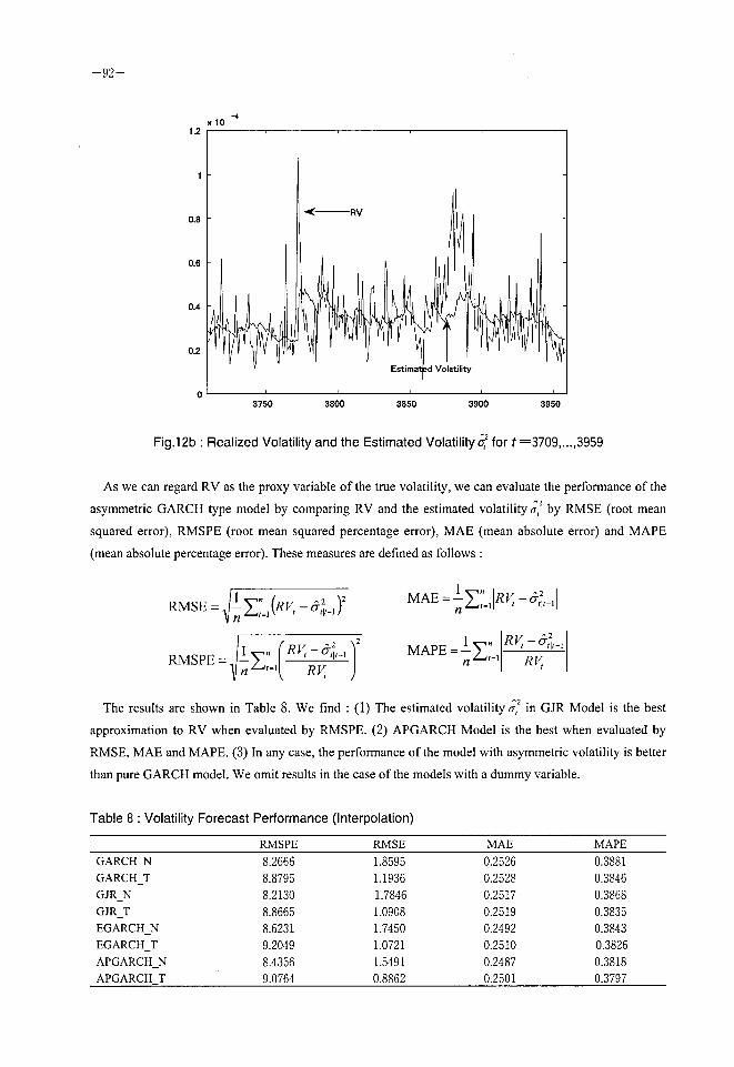
3750 3800 3850 3900 3950
Fig.12b : Realized Volatility and the Estimated Volatilitya* for t=3709 3959
As we can regard RV as the proxy variable of the true volatility, we can evaluate the performance of theasymmetric GARCH type model by comparing RV and the estimated volatility a] by RMSE (root mean
squared error), RMSPE (root mean squared percentage error), MAE (mean absolute error) and MAPE
(mean absolute percentage error). These measures are defined as follows :
Rmse=JIz;>f,-^_,)2 MAE4^-
MAPE=-Y"
Rv-ai
R MSPE= -V1 1-^>=1
1á" (RV,-&>
n^-"\ RV,
RV. -&L,
RV,
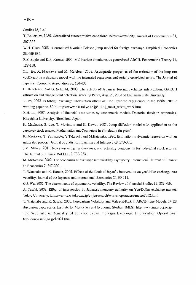
The results are shown in Table 8. We find : (1) The estimated volatility a, in GJR Model is the best
approximation to RV when evaluated by RMSPE. (2) APGARCH Model is the best when evaluated by
RMSE, MAE and MAPE. (3) In any case, the performance of the model with asymmetric volatility is better
than pure GARCH model. We omit results in the case of the models with a dummy variable.
Table 8 : Volatility Forecast Performance (Interpolation)R M S P E R M S E M A E M A P E
G A R C H N 8 .2 6 6 6 1 .8 5 9 5 0 .2 5 2 6 0 .3 8 8 1
G A R C H T 8 .8 7 9 5 1 . 1 9 3 6 0 .2 5 2 8 0 .3 8 4 6
G J R N 8 .2 1 3 0 1 .7 8 4 6 0 .2 5 1 7 0 .3 8 6 8
G J R T 8 .8 6 6 5 1 .0 9 0 8 0 .2 5 1 9 0 .3 8 3 5
E G A R C H N 8 .6 2 3 1 1 .7 4 5 0 0 .2 4 9 2 0 .3 8 4 3
E G A R C H T 9 .2 0 4 9 1 .0 7 2 1 0 .2 5 1 0 0 .3 8 2 6
A P G A R C H N 8 .4 3 5 6 1 .5 4 9 1 0 .2 4 8 7 0 .3 8 1 8
A P G A R C H T 9 .0 7 6 4 0 .8 8 6 2 0 .2 5 0 1 0 .3 7 9 7

-93-
3. 4 Intervention Effect on RVNext we detect the intervention effect on RV by the following equation :
RV= a0+ a,£]_,+ a2RV,_1+ a,D,, (D
where D, is the same dummy variable in Section 3.2 to represent the intervention by BOJ. e, is the OLS
residual calculated from Ito Equations (2) and (3) in the next section 4.1 and the simplest mean equation of
the return : r,=c+ e,. The estimated parameters of so, « 1, ff!, ff3, calculated by using the above three kinds
of residuals £, are shown in Tables 9-ll.
Table 9 : Estimated Parameters in Model (1) Based on OLS Residual from Model (2)
C o e f fi c ie n t S td . E rr o r t- S ta tis t ic P r o b .
2 .3 3 E - 0 5 1 .1 9 E - 0 6 1 9 .6 4 3 0 7 0 .0 0 0 0
0 .2 7 6 2 7 4 0 .0 0 8 5 8 6 3 2 . 1 7 6 7 0 0 .0 0 0 0
0 .3 8 1 3 2 2 0 .0 1 2 9 8 9 2 9 .3 5 7 1 9 0 .0 0 0 0
1 .3 9 E - 0 5 3 .3 2 E - 0 6 4 . 1 9 6 5 5 4 0 .0 0 0 0
R -s q u a r e d 0 .4 7 3 0 9 9 M e a n d e p e n d e n t v a r 6 .0 0 E - 0 5
A d j u s t e d R - s q u a re d 0 .4 7 2 6 9 9 S . D . d e p e n d e n t v a r 8 .0 4 E - 0 5
S .E . o f r e g r e s s io n 5 .8 4 E - 0 5 A k a ik e i n fo c ri te r io n - 1 6 .6 5 6 9 7
S u m s q u a re d re s i d 1 .3 5 E - 0 5 S c h w a rz c r ite r io n - 1 6 .6 5 0 6 2
L o g l ik e l ih o o d 3 2 9 5 1 .5 0 D u r b in - W a ts o n s ta t 2 .1 6 6 6 7 9
T a b le 1 0 : E s t im a t e d P a r a m e t e r s in M o d e l ( 1 ) B a s e d o n O L S R e s id u a l f r o m M o d e l ( 3 )
C o e f f ic ie n t S td . E r ro r t- S t a t is tic p ro b .
2 .3 7 E -0 5 1 .2 0 E -0 6 1 9 .7 3 3 3 9 0 .0 0 0 0
0 .2 5 6 1 3 6 0 .0 0 8 4 7 9 3 0 .2 1 0 0 6 0 .0 0 0 0
0 .3 8 7 9 5 0 0 .0 1 3 1 9 4 2 9 .4 0 3 3 8 0 .0 0 0 0
1 .4 5 E -0 5 3 .3 6 E -0 6 4 .3 2 4 6 3 9 0 .0 0 0 0
R - s q u a r e d 0 .4 5 9 8 1 0 M e a n d e p e n d e n t v a r 6 .0 0 E - 0 5
A d j u s te d R - s q u a r e d 0 .4 5 9 4 0 0 S . D . d e p e n d e n t v a r 8 .0 4 E - 0 5
S .E . o f re g r e s s i o n 5 .9 1 E -0 5 A k a ik e in f o c r ite r io n - 1 6 .6 3 2 0 7
S u m s q u a r e d r e s id 1 .3 8 E -0 5 S c h w a rz c ri te r io n - 1 6 .6 2 5 7 1
L o g lik e lih o o d 3 2 9 0 2 .2 3 D u r b in - W a ts o n s t a t 2 .1 6 5 4 5 5
T a b le l l : E s t im a t e d P a ra m e t e rs i n M o d e l ( 1 ) B a s e d o n O L S R e s id u a l f r o m r , = c + e ,
C o e f fi c ie n t S t d . E r r o r t - S ta tis ti c P ro b .
2 .4 1 E - 0 5 1 .2 1 E - 0 6 1 9 .9 4 6 1 1 0 .0 0 0 0
0 .2 3 9 8 8 8 0 .0 0 8 2 4 9 2 9 .0 7 9 3 7 0 .0 0 0 0
0 .3 8 9 0 9 0 0 .0 1 3 3 5 7 2 9 .1 2 9 7 1 0 .0 0 0 0
1 .5 4 E - 0 5 3 .3 8 E - 0 6 4 .5 4 6 3 1 2 0 .0 0 0 0
R - s q u a re d 0 .4 5 2 2 3 8 M e a n d e p e n d e n t v a r 6 .0 0 E - 0 5
A d j u s te d R - s q u a r e d 0 .4 5 1 8 2 2 S . D . d e p e n d e n t v a r 8 .0 4 E - 0 5
S .E . o f r e g r e s s io n 5 .9 6 E - 0 5 A k a ik e in f o c r it e r io n - 1 6 .6 1 8 4 0
S u m s q u a r e d r e s id 1 .4 0 E - 0 5 S c h w a r z c r ite ri o n - 1 6 .6 1 2 0 5
L o g lik e lih o o d 3 2 8 8 3 .5 0 D u rb i n -W a t s o n s ta t 2 . 1 5 6 5 2 8
From these tables we can see that a3 is around 1.4X10 and significant, which means that the
intervention by BOJ has positive effect on RV.

-94-
4 Asymmetric Effect of the Intervention on the Mean Equation4. 1 Estimation ofIto Model
So far have we focused on the variance equation to determine whether BOJ' s intervention has any
asymmetric effect on the volatility and introduced a variable to represent the asymmetric effect in the
variance equation. In this section we change our standpoint from the variance equation to the mean equation
of the volatility model to see if the intervention has asymmetric effects in the mean equation. To do so we
introduce the amount of intervention as an explanatory variable directly in the mean equation. Instead we
use the symmetric variance equation. Along this line Ito (2002) proposed the following model with GARCH
(1,1) error term :
*,-Vi= l%+ /?,k-i-V2)+ &(Vi-*r,-i)+ /?M+ PJntF,+ PJntI,+ e, (2)
where
e,=z,a with z~N(0,l), a]= ao+ a,e2,_,+ a\_v
s, : log of spot rate ofdayt,
s , : log of long-run equilibrium exchange rate, 125 yen (following Ito, 2002, we set long-run equilibrium at
125 ¥/$, because 125 ¥/$ was the dividing line between yen selling and purchasing),
Int : the Japanese intervention (in 100 million yen),
IntF : the US intervention by Federal Reserve Board (FRB, in million dollars),
IntI : the initial intervention (Int: if no intervention in 5 proceeding business days; 0: otherwise).
The initial intervention and the exchange rate are shown in Fig.13. If the interventions by BOJ are
effective, then we expect /?3<0. For example, if the yen-purchasing intervention (Int>0) by BOJ tends to
appreciate the yen st-5,_,<0, then the negative sign of /?3 should be obtained. The US interventions
(positive for yen purchasing) are judged to be effective when /?4 is negative. The total effects of the joint
interventions are measured by /?3+ /?4. Because all of the US interventions were joint interventions, the
magnitude of [it may contain any of the nonlinear effects of the joint interventions. The coefficient of y?5
shows the effectiveness of the first intervention in more than a week beyond just as one of the interventions.
Such a variable is originally introduced by Humpage (1998). The full impact of the first intervention is
measured by /33+ /?5.
We basically follow the Ito model but the data ofIntF are not available for us. As a result we had to omit
IntF and hence our model is written as
*,-*,-.= /?»+ Aft-i-s,-2)+ ft(s,-i-*r,-.)+ PM+ PJ"tI,+ *, (3)
where we assume e, follows GARCH (1,1) as in Model (2). The estimated parameters of Model (3) are
shown in Table 12.

-95-
Table 12 : Estimation of GARCH (1 ,1) Model (3) for the Whole Sample Period (1991/05/01-2006/08/31)
Coefficient Std. Error t-Statistic Prob.
p . . -0 .0 0 0 2 8 0 0 .0 0 0 1 2 7 - 2 .2 0 4 5 9 6 0 .0 2 7 5
P i -0 .0 0 4 7 7 9 0 .0 1 5 9 5 7 - 0 .2 9 9 5 2 8 0 .7 6 4 5
P i -0 .0 0 2 3 7 2 0 .0 0 1 0 1 7 - 2 .3 3 2 1 1 5 0 .0 1 9 7
p . , - 3 .2 4 E -0 7 9 .4 0 E - 0 - 3 .4 4 4 6 2 4 0 .0 0 0 6
/サ s - 7 .7 5 E -0 6 1 .5 8 E - 0 7 - 4 .8 9 2 4 4 2 0 .0 0 0 0
a o 7 .6 4 E - 0 7 1 .2 0 E - 0 7 6 .3 9 4 5 6 9 0 .0 0 0 0
- 1 0 .0 4 6 2 6 9 0 .0 0 3 8 3 4 1 2 .0 6 7 5 5 0 .0 0 0 0
<* , 0 .9 3 7 2 7 3 0 .0 0 5 4 9 1 1 7 0 .6 9 4 8 0 .0 0 0 0
160
140
120 h
ioo |-
5000
-\ -5000
-| -10000
-1 50000 500 1 000 1 500 2000 2 500 3000 3 500 4000
Fig. 13 : The ¥/$ Exchange Rate and Japanese Initial Intervention from 1991/05/01 to 2006/08/31
4. 2 VariantsofIto Model
As depicted in the previous sections there are extreme returns and RVs at Russian economic crisis. To
deal with these extreme values we introduce a dummy variable, D, , in which 1 is assigned for 1998/10/07,
1998/10/08, 1998/10/09, and 0 elsewhere. By using this dummy variable we rewrite Ito Model (3) as
follows:
5,-5,_,= /? + (3i(.s,_1-s,_2)+ &(*,_,-/,_,)+ /?M+ /35^'/,+ /?eA+ e, (4)
The estimates of the Equation (4) are shown in Table 13. As is seen the estimated coefficient for /?6 is
significant. Comparing Table 13 with Table 12, we notice that the significance level of /?j is slightly
improved in Table 13, and /?5 becomes much smaller in Table 13.

-96-
Table 13 : Estimation of GARCH (1,1) Model (4) forthe Whole Sample Perio (1991/05/01-2006/08/31)C o e f f ic ie n t S td . E rr o r t- S ta ti st ic P r o b .
p . -0 .0 0 0 2 7 6 0 .0 0 0 1 2 7 - 2 .1 7 7 1 0 1 0 .0 2 9 5
」 . -0 .0 1 2 0 3 1 0 .0 1 6 0 5 5 - 0 .7 4 9 3 7 0 0 .4 5 3 6
K -0 .0 0 2 3 6 0 0 .0 0 1 0 1 6 - 2 .3 2 3 1 2 1 0 .0 2 0 2
p , - 3 .2 3 E - 0 7 9 .3 9 E - 0 8 -3 .4 4 0 4 0 3 0 .0 0 0 6
p , - 7 .7 0 E - 0 7 1 .5 8 E - 0 7 -4 .8 6 9 7 9 7 0 .0 0 0 0
t* > - 0 .0 3 8 0 6 1 0 .0 0 4 8 3 3 -7 .8 7 4 8 9 4 0 .0 0 0 0
a o 7 .2 7 E - 0 7 1 . 1 6 E - 0 7 6 .2 6 4 1 0 6 0 .0 0 0 0
ff > 0 .0 4 3 2 7 4 0 .0 0 3 7 0 5 1 1 .6 7 8 7 6 0 .0 0 0 0
a 0 .9 4 0 7 6 2 0 .0 0 5 2 7 0 1 7 8 .5 0 3 1 0 .0 0 0 0
The RV and the estimated volatility <r,2 in Model (4) are compared in Fig.l4a and Fig.l4b, which show
the observed RV and the estimated a] respectively. By comparing these two graphs we can see that the
estimated variance a, can capture the movement of RV to a certain extent.
Fig.14a : Realized Volatility in Model (4)
3500 4000
-Ertlmfd Volatility
\^^k]\u^\^j^ y^ww,^1 600 2000 2BO0 3000 3600 4OO0
Fig.14b : Estimated Volatility of in Model (4)

-97-
Next we introduce a dummy variable AD, to capture FRB intervention such as
1 intervention byFRBAD,=-
0 nointervention
and estimated GARCH Model (5) for the whole sample period (1991/05/01- 2006/08/31).
J,-V,=&+ ;9.(Vi-V2)+ /32(^-1-/,-1)+ PM+ PJntI,+ [3fi,+ fi,AD,+ e, (5)
As shown in Table 14 the coefficient /37 is not significant, which means the intervention by FRB may not be
effective.
Table 14 : Estimation of GARCH (1,1) Model (5) forthe Whole Sample Period
(1 991/05/01 -2006/08/31 , with a Dummy Variable for FRB Intervention)
C o e f f ic i e n t S td . E r ro r t- S t a t is tic P r o b .
/? ォ - 0 .0 0 0 2 7 4 0 .0 0 0 1 2 7 - 2 .1 4 9 4 3 0 0 .0 3 1 6
0 . - 0 .0 1 2 2 1 1 0 .0 1 6 0 3 6 - 0 .7 6 1 4 3 3 0 .4 4 6 4
p , - 0 .0 0 2 3 8 3 0 .0 0 1 0 1 8 - 2 .3 4 1 1 6 5 0 .0 1 9 2
p , - 3 .2 4 E -0 7 9 .3 8 E - 0 - 3 .4 4 8 7 1 8 0 .0 0 0 6
h - 7 .7 2 E -0 7 1 .5 8 E - 0 7 -4 .8 7 2 9 0 5 0 .0 0 0 0
? t -0 .0 3 8 0 6 6 0 .0 0 4 8 2 3 - 7 .8 9 1 9 0 2 0 .0 0 0 0
/' , -0 .0 0 1 0 0 2 0 .0 0 0 7 1 2 - 1 .4 0 8 3 2 4 0 . 1 5 9 0
a o 7 .1 5 E - 0 7 1 .1 6 E - 0 7 6 .1 5 3 1 9 9 0 .0 0 0 0
a l 0 .0 4 2 7 8 3 0 .0 0 3 8 4 6 l l . 1 2 2 9 9 0 .0 0 0 0
a . 0 .9 4 1 5 0 2 0 .0 0 5 4 2 1 1 7 3 .6 7 8 3 0 .0 0 0 0
Although we could not obtain the data ofFRB intervention we can estimate it by subtracting the BOJ
intervention from the total intervention (FRB+BOJ intervention). This indirect calculation of FRB
intervention, denoted by IntF,, is somewhat problematic, but may provide useful information. We estimated
GARCH Model (6) by using IntF, for the whole sample period (1991/05/01- 2006/08/31), and the results are
shown in Table 15. From this table we can see that the estimated coefficient for IntF, is significant and /93+
/34<0, which means thejoint intervention by FRB and BOJ was effective.
å s,--Vi=/? + ^(s,-ls,_2)+ i3,^1-sT,_1)+ pjnt,+ pjntF,+ pjntl,+ pjD,+ e, (6)
Table 15 : Estimation of GARCH (1,1) Model (6) forthe Whole Sample Period
(1991/05/01-2006/08/31 , with the Intervention by FRB)
C o e ff ic ie n t S td . E r r o r t- S t a t is tic P r o b .
/? 0 - 0 .0 0 0 2 5 1 0 .0 0 0 1 2 8 - 1 .9 6 3 8 9 1 0 .0 4 9 5
/' . - 0 .0 1 4 1 7 9 0 .0 1 6 1 8 0 - 0 .8 7 6 3 3 4 0 .3 8 0 8
? , - 0 .0 0 1 9 9 3 0 .0 0 1 0 3 6 - 1 .9 2 3 4 8 5 0 .0 5 4 4
p , - 3 .1 7 E -0 7 9 .3 6 E - 0 - 3 .3 9 2 2 9 6 0 .0 0 0 7
p t - 1 .4 3 E -0 5 1 .9 8 E - 0 6 - 7 .2 2 8 3 3 3 0 .0 0 0 0
p > - 7 .3 9 E -0 7 1 .6 3 E - 0 7 -4 .5 4 0 9 2 4 0 .0 0 0 0
/' . -0 .0 3 8 1 5 5 0 .0 0 4 7 6 7 -8 .0 0 4 0 1 8 0 .0
a o 6 .9 5 E - 0 7 1 .1 3 E - 0 7 6 . 1 4 8 7 5 1 0 .0 0 0 0
a l 0 .0 4 1 3 6 6 0 .0 0 3 9 8 4 1 0 .3 8 2 4 3 0 .0 0 0 0
a ; 0 .9 4 3 2 1 4 0 .0 0 5 4 6 3 1 7 2 .6 5 6 7 0 .0 0 0 0

Wealso used the total intervention by FRB and BOJ denoted by IntT, and estimated GARCH (1,1) Model
(7). As shown in Table 16 the coefficient /?7 for IntT, is significant, which means the total intervention is
effective.
s,-s,.i= /?o+ /91(Vi-V2)+ A>C*,-i"^-i)+ PM+ P-J»tl,+ {16D,+ pjntT, e, (7)
Table 16 : Estimation of GARCH (1,1) Model (7) for the Whole Sample Period
(1991/05/01 -2006/08/31 , with the Total Intervention by FRB and BOJ)
C o e ff ic ie n t S td . E r r o r t- S t a t is tic P ro b .
/サ . - 0 .0 0 0 2 5 2 0 .0 0 0 1 2 7 - 1 .9 8 1 4 3 9 0 .0 4 7 5
/? , - 0 .0 1 4 0 9 0 0 .0 1 6 1 0 4 - 0 .8 7 4 9 6 1 0 .3 8 1 6
/ォ 2 - 0 .0 0 2 0 2 8 0 .0 0 1 0 3 0 - 1 .9 6 8 3 8 1 0 .0 4 9 0
p , -3 .1 8 E - 0 7 9 .3 7 E -0 - 3 .3 9 0 1 9 5 0 .0 0 0 7
P i -7 .3 5 E - 0 7 1 .7 3 E -0 7 - 4 .2 4 6 3 0 2 0 .0 0 0 0
p . - 0 .0 3 8 1 4 3 0 .0 0 4 7 5 0 - 8 .0 3 0 1 4 1 0 .0 0 0 0
/? 7 -4 .7 8 E - 0 6 3 .9 5 E -0 7 - 1 2 . 1 0 6 2 4 0 .0 0 0 0
" o 6 .8 0 E -0 7 1 . l l E -0 7 6 .1 1 3 3 8 1 0 .0 0 0 0
ff l 0 .0 4 0 6 3 3 0 .0 0 3 8 5 9 1 0 .5 2 9 6 8 0 .0 0 0 0
a 0 .9 4 4 2 9 2 0 .0 0 5 2 3 3 1 8 0 .4 4 5 3 0 .0 0 0 0
Table 17 shows the results of the estimation of Ito Model (2) for the whole sample period (1991/05/01-
2006/08/31).
Table 17 : Estimation of GARCH (1,1) Type Ito Model (2) for the Whole Sample Period
(1 991 /05/01 -2006/08/31 )C o e f f i c i e n t S t d . E r r o r t - S t a t i s t i c P r o b .
P o - 0 .0 0 0 2 5 6 0 . 0 0 0 1 2 8 - 2 .0 0 0 3 9 0 0 . 0 4 5 5
0 . - 0 .0 0 6 8 4 2 0 . 0 1 6 0 1 6 - 0 .4 2 7 1 7 1 0 . 6 6 9 3
p , - 0 .0 0 2 0 1 1 0 . 0 0 1 0 3 6 - 1 .9 4 1 7 8 8 0 . 0 5 2 2
/3 3 - 3 . 1 8 E - 0 7 9 .3 7 E - 0 8 - 3 .3 9 6 2 1 9 0 . 0 0 0 7
P i - 1 . 4 1 E - 0 5 2 .0 2 E - 0 6 - 6 .9 8 1 8 9 8 0 .0 0 0 0
P s - 7 . 4 5 E - 0 7 1 . 6 3 E - 0 7 - 4 . 5 6 9 3 3 6 0 .0 0 0 0
" o 7 . 3 3 E - 0 7 1 . 1 7 E - 0 7 6 .2 4 7 5 1 4 0 .0 0 0 0
ォ 1 0 .0 4 4 3 8 4 0 .0 0 4 0 4 4 1 0 . 9 7 6 5 3 0 .0 0 0 0
ォ , 0 .9 3 9 6 5 3 0 .0 0 5 6 7 0 1 6 5 .7 3 2 3 0 .0 0 0 0
4.3 F-test
To see the intervention effect we apply a variance analysis by F-test. We divide sample period into "in
sample" before the intervention and "out of sample" ("out sample" for short) after that. We compare "in
sample variance" and "out of sample variance". If F-test indicates the variance is unchanged in the two
sample periods we may say there is no intervention effect. We apply F-test to the period including Russian
economic crisis in August 1998. In October 1998 there was a striking aftershock when huge amount of
Japanese Yen was bought back by hedge funds. The aftershock was seen as a big downward spike in Fig.6.
Wechoose the period of 1998/08/24 - 1998/12/22 as a whole sample period and divide this period into two
periods: 1998/08/24-1998/10/05 as "in sample" and 1998/10/10-1998/12/22 as "out sample".
F =-'f- =1.15 , where a ] and a 2mlare the estimated variances in "in sample" and "out sample" period

-99-
respectively. As the degree of freedom in denominator and numerator are very large, F= 1.15 is significant.
As the result we can say the variances are not equal in the two sample periods. This means that the volatility
became smaller after the Russian economic crisis.
5 Concluding remarksIn this article, we have analyzed the asymmetric effect of the intervention of BOJ in the foreign Exchange
Market through GARCH models. The effect may be seen in the volatility equation and/or the mean equation
of the GARCH models. First, to determine whether there is any asymmetric effect on volatility of the
returns of exchange rate, we have applied GJR, EGARCH and APGARCH models, which can reflect
asymmetry of the volatility in keeping the mean equation constant. We name this approach 'variance
equation approach'. Second, to determine whether the intervention has an effect on the mean equation, we
have applied Ito (2002) model and its variants to the real data in assuming that the variance equation is
symmetric. We namethis approach 'mean equation approach'. We have also applied F-test approach to test
the effect of the intervention of BOJ. In the variance equation approach, we tested if the intervention of BOJ
has any asymmetric effect on the volatility through the dummy variable D, in the right side of the variance
equations, which takes a value 1 for the intervention and 0 elsewhere. We obtained the significant estimate
of the coefficient ofD, , and we can say that the intervention has an effect on the exchange rate volatility. In
the mean equation approach, we used Ito model with symmetric GARCH error and with the amount of
intervention as an explanatory variable in the mean equation. Especially, we used RV analysis based on
high-frequency exchange rate data. In the F-test approach, we obtained the empirical evidence, which
supports that the intervention by BOJ makes the exchange rate volatility more fluctuate. The interventions
by BOJ have effects in the case of Russian economic crisis.
As our empirical study showed that the intervention by BOJ has significant asymmetric effects on the
volatility and the mean equations of the returns of exchange rate, we may conclude that the intervention by
BOJ does not have a stabilizer effect on the volatility of returns of exchange rate.
AcknowledgementThis article is the extension of the Chapter 4 of my doctoral dissertation, Analysis ofFinancial Time
Series by Econometric Models, which was written under the guidance by Professor Koichi Maekawa and
submitted to the Graduate School of Social Science at Hiroshima University. I am especially grateful to
Professor Koichi Maekawa, who is now at Hiroshima University of Economics, for his suggestions and
comments on my doctoral dissertation and this article. I also would like to thank Toshiaki Watanabe,
Institute of Economic Research, Hitotsubashi University, for his helpful comments and to Tee Kian Heng,
Faculty of Policy Studies, Iwate Prefectural University, for his help with data-processing. All errors are my
own.
ReferencesD. Avramov, T. Chordia and A. Goyal, 2006. The impact of trades on daily volatility. Review ofFinancial
Studies 19, 1241-1277.
G. Bekaert and G.J. Wu, 2000. Asymmetric volatility and risk in equity markets. The Review ofFinancial
-100-
Studies 13, 1-42.
T. Bollerslev, 1986. Generalized autoregressive conditional heteroskedasticity. Journal of Econometrics 31,
307-327.
W.H.Chan, 2003. A correlated bivariate Poisson jump model for foreign exchange. Empirical Economics
28,669-685.
R.F. Engle and K.F. Kroner, 1995. Multivariate simultaneous generalized ARCH. Econometric Theory ll,
122-150.
Z.L. He, K. Maekawa and M. McAleer, 2003. Asymptotic properties of the estimator of the long-run
coefficient in a dynamic model with the integrated regressors and serially correlated errors. The Journal of
Japanese Economic Association 54, 420-438.
E. Hillebrand and G. Schnabl, 2003. The effects of Japanese foreign exchange intervention: GARCH
estimation and change point detection. Working Paper, Aug. 29, 2003 of Louisiana State University.
T. Ito, 2002. Is foreign exchange intervention effective?: the Japanese experiences in the 1990s. NBER
working paper no. 89 14. http://www.e.u-tokyo.ac.jp/~tito/j_most_recent_work.htm.
X.H. Lu, 2007. Analysis of financial time series by econometric models. Doctorial thesis in economics.
Hiroshima University, Hiroshima, Japan.
K. Maekawa, S. Lee, T. Morimoto and K. Kawai, 2007. Jump diffusion model with application to the
Japanese stock market. Mathematics and Computers in Simulation (in press).
K. Maekawa, T. Yamamoto, Y.Takeuchi and M.Hatanaka, 1996. Estimation in dynamic regression with an
integrated process. Journal of Statistical Planning and Inference 49, 279-303.
J.M. Maheu, 2004. News arrival, jump dynamics, and volatility components for individual stock returns.
The Journal ofFinance Vol.LIX, 2, 755-973.
M.McKenzie, 2002. The economics of exchange rate volatility asymmetry. International Journal of Finance
an Economics 7, 247-260.
T. Watanabe and K. Harada, 2006. Effects of the Bank ofJapan' s intervention on yen/dollar exchange rate
volatility. Journal of the Japanese and International Economies 20, 99-1 1 1.
G.J. Wu, 2001. The determinants of asymmetric volatility. The Review ofFinancial Studies 14, 837-859.
A. Tasaki, 2002. Effect of intervension by Japanese monetary authority on Yen/Dollar exchange market.
Tokyo University. http://www.e.u-tokyo.ac.jp/cirj e/research/workshops/macro/macro2002.html.
T. Watanabe and K. Sasaki, 2006. Forecasting Volatility and Value-at-Risk in ARCH- type Models. IMES
discussion paper series. Institute for Moneytary and Economic Studies (IMES). http: www.imes.boj.or.jp.
The Web site of Ministry of Finance Japan, Foreign Exchange Intervention Operations:
http ://www.mof.go.jp/l c02 1.htm.