ABSTRACT

Title of Document: AERODYNAMIC ANALYSIS OF AN MAV-

SCALE CYCLOIDAL ROTOR SYSTEM

USING A STRUCTURED OVERSET RANS

SOLVER

Kan Yang, Master of Science, 2010

Directed By: Dr. James D. Baeder, Associate Professor,

Department of Aerospace Engineering

A compressible Reynolds-Averaged Navier-Stokes solver was used to investigate the

performance and flow physics of the cycloidal rotor (cyclocopter). This work

employed a computational methodology to understand the complex aerodynamics of

the cyclocopter and its relatively unexplored application for MAVs. The numerical

code was compared against performance measurements obtained from experiment

and was seen to exhibit reasonable accuracy. With validation of the flow solver, CFD

predictions were used to gain qualitative insight into the flowfield. Time histories

revealed large periodic variations in thrust and power. In particular, the virtual

camber effect was found to significantly influence the vertical force time history.

Spanwise thrust and flow visualizations showed a highly three-dimensional flowfield

with large amounts of blade shedding and blade-vortex interaction. Overall, the

current work seeks to provide unprecedented insight into the cyclocopter flowfield

with the goal of developing an accurate predictive tool to refine the design of future

cyclocopter configurations.

Aerodynamic Analysis of an MAV-Scale

Cycloidal Rotor System Using a

Structured Overset RANS Solver

by

Kan Yang

Thesis submitted to the Faculty of the Graduate School of theUniversity of Maryland at College Park in partial fulfillment

of the requirements for the degree ofMaster of Science

2010

Advisory Committee:

Dr. James D. Baeder, Chairman/AdvisorDr. Inderjit ChopraDr. Kenneth Yu

c© Copyright by

Kan Yang

2010

Dedication

To my parents and stepparents, without whom none of this would

be possible.

ii

Acknowledgements

I am incredibly grateful to my advisor, Dr. James Baeder, who has been

consistently supportive throughout the course of this work, and from whom I

have received so much invaluable academic advice over the past two years. He

has helped steer me from confusion and uncertainty as a fresh Bachelors graduate

to direction and confidence in my ability to conduct research. With his guidance,

I feel much more prepared to tackle obstacles in my future career path, and I

feel privileged to have been his student.

I am also extremely indebted to Vinod for his immeasurable help and advice

over the past two years. Through thick and thin in the “dark” days of my

research, and even during the countless times when I suffered lapses in judgment

and asked unreasonable questions, he has always shown an incredible amount

of patience in dealing with my problems. I hold him in the highest academic

regard and wish him all the best with his professorship; I am certain that he will

inspire students for years to come.

I would like to thank Moble, who at every step along the way has helped me

to clarify my doubts and better understand my research topic. I also express

deep gratitude to Shreyas, who has assisted me with my work and provided

excellent suggestions in matters concerning both academia and life. I would like

to show appreciation for my committee members Dr. Yu and Dr. Chopra in

providing valuable recommendations to help improve my thesis. In addition, I

am extremely grateful to Dr. Winkelmann for his wisdom, good humor, and

kindness during my first semester at Maryland.

To Aisa, Amie, Christian, and Mary: though we may be separated by vast

iii

distances, your warmth and spirit have kept me going over the past two years. I

honestly could not ask for better friends. May and Eddie, who I have known the

longest: thank you for all the wonderful memories. You both have helped define

such a significant part of who I am. Sebastian, Pranay, Shivaji and Taran: I

am incredibly glad to have met all of you, and your friendship has enriched my

life here at Maryland. Evan, Sonia, Scott, Jared, Erica, and Jesse: thank you

for being such fantastic roommates, and for putting up with my quirks. You

have made coming home everyday something I really look forward to. Also, I

thank Chen, Mor, Graham, Mel, Brandon, Ben, Ananth, Tim, Kayla, Ron, An-

drei, Yashwant, Erika, and Ramya for their camaraderie, support, and incredible

generosity.

Finally, I must thank my father, mother, stepfather, and stepmother for all

the compassion and love that they have given me. Since childhood, their devotion

and encouragement has always been the backbone from which I could grow and

strive for my dreams. Without them, I would not be where I am today.

iv

Table of Contents

List of Tables ix

List of Figures x

Nomenclature xiv

1 Introduction 1

1.1 Problem Statement . . . . . . . . . . . . . . . . . . . . . . . . . . 1

1.1.1 Definition of a Cycloidal Rotor System . . . . . . . . . . . 2

1.2 Previous Work . . . . . . . . . . . . . . . . . . . . . . . . . . . . 3

1.2.1 Experimental Work on Full-Scale Cycloidal Rotors . . . . 3

1.2.2 Interim work on Cycloidal Wind Turbines . . . . . . . . . 6

1.2.3 Experimental Work on MAV-Scale Cycloidal Rotors . . . . 8

1.2.4 Analytical Models of MAV-Scale Cycloidal Rotors . . . . . 10

1.2.5 CFD Studies of MAV-Scale Cycloidal Rotors . . . . . . . . 12

1.3 Objective of Current Work . . . . . . . . . . . . . . . . . . . . . . 13

1.4 Thesis Outline . . . . . . . . . . . . . . . . . . . . . . . . . . . . . 14

1.5 Key Contributions of the Current Work . . . . . . . . . . . . . . . 15

v

2 Methodology 16

2.1 Grid Generation Methods . . . . . . . . . . . . . . . . . . . . . . 17

2.1.1 Algebraic Grid Generation . . . . . . . . . . . . . . . . . . 18

2.1.2 Hyperbolic Grid Generation . . . . . . . . . . . . . . . . . 21

2.2 Overset Grid Methodology . . . . . . . . . . . . . . . . . . . . . . 22

2.3 Grid Motion . . . . . . . . . . . . . . . . . . . . . . . . . . . . . . 24

2.3.1 Grid Rotation . . . . . . . . . . . . . . . . . . . . . . . . . 25

2.3.2 Numerical Approximation of the Four-Bar Pitching Mech-

anism . . . . . . . . . . . . . . . . . . . . . . . . . . . . . 25

2.3.3 Blade Deformations . . . . . . . . . . . . . . . . . . . . . . 27

2.4 Flow Solver . . . . . . . . . . . . . . . . . . . . . . . . . . . . . . 29

2.4.1 Compressible Navier-Stokes Equations . . . . . . . . . . . 29

2.4.2 Reynolds-Averaged Navier-Stokes Equations . . . . . . . . 33

2.4.3 Turbulence Model . . . . . . . . . . . . . . . . . . . . . . . 35

2.4.4 Spatial Discretization . . . . . . . . . . . . . . . . . . . . . 36

2.4.5 Preconditioning . . . . . . . . . . . . . . . . . . . . . . . . 38

2.4.6 Implicit Time Marching and Dual Time-Stepping . . . . . 39

2.4.7 Boundary Conditions . . . . . . . . . . . . . . . . . . . . . 40

2.4.8 Specific Methods used in OVERTURNS . . . . . . . . . . 43

2.5 Summary . . . . . . . . . . . . . . . . . . . . . . . . . . . . . . . 43

3 Validation of the Flow Solver 46

3.1 Steady Airfoil Validation . . . . . . . . . . . . . . . . . . . . . . . 47

3.2 Unsteady Pitching Airfoil Validation . . . . . . . . . . . . . . . . 50

3.3 Validation of 2-D Unsteady Flow Separation from Airfoil Rotation 54

3.3.1 Dynamic Stall Flow Visualization . . . . . . . . . . . . . . 55

vi

3.3.2 Comparison of Normal and Tangential Force Coefficients . 57

3.4 Summary . . . . . . . . . . . . . . . . . . . . . . . . . . . . . . . 58

4 Comparison of Cycloidal Rotor CFD Results with Experiment 60

4.1 Experimental Setup for Validation . . . . . . . . . . . . . . . . . . 60

4.1.1 Flow Visualization . . . . . . . . . . . . . . . . . . . . . . 62

4.2 2-D and 3-D Grid Systems . . . . . . . . . . . . . . . . . . . . . . 63

4.3 Cyclocopter Blade Deformations . . . . . . . . . . . . . . . . . . . 65

4.4 Performance Comparisons . . . . . . . . . . . . . . . . . . . . . . 67

4.4.1 Thrust and Aerodynamic Power Comparisons . . . . . . . 68

4.4.2 Velocity Vectors . . . . . . . . . . . . . . . . . . . . . . . . 74

4.5 Summary . . . . . . . . . . . . . . . . . . . . . . . . . . . . . . . 77

5 CFD Predictions 79

5.1 Variation in Force and Power Over Time . . . . . . . . . . . . . . 80

5.1.1 Vertical Force and Aerodynamic Power Variation over Time 82

5.1.2 Sidewise Force Variation over Time . . . . . . . . . . . . . 83

5.1.3 Comparison Between Deformed and Undeformed Blades . 84

5.1.4 Cambered Airfoil Analysis . . . . . . . . . . . . . . . . . . 85

5.2 Spanwise Thrust Distribution . . . . . . . . . . . . . . . . . . . . 89

5.3 Time-Averaged Inflow Distribution . . . . . . . . . . . . . . . . . 93

5.4 Flow Visualization . . . . . . . . . . . . . . . . . . . . . . . . . . 97

5.5 Summary . . . . . . . . . . . . . . . . . . . . . . . . . . . . . . . 98

6 Conclusions 103

6.1 Summary . . . . . . . . . . . . . . . . . . . . . . . . . . . . . . . 104

6.2 Specific Observations . . . . . . . . . . . . . . . . . . . . . . . . . 105

vii

6.3 Future Work . . . . . . . . . . . . . . . . . . . . . . . . . . . . . . 107

A Numerical Work on Cycloidal Wind Turbines 110

A.1 Numerical Work in Literature on VAWT and CWT . . . . . . . . 110

A.1.1 Simple Analytical Models . . . . . . . . . . . . . . . . . . 110

A.1.2 CFD Simulations . . . . . . . . . . . . . . . . . . . . . . . 111

A.1.3 Other Numerical Studies . . . . . . . . . . . . . . . . . . . 112

A.2 Preliminary CFD Validation in the Current Work . . . . . . . . . 112

A.2.1 Cycloidal Wind Turbine Validation . . . . . . . . . . . . . 113

A.2.2 Tangential Force Comparison . . . . . . . . . . . . . . . . 114

A.2.3 Summary . . . . . . . . . . . . . . . . . . . . . . . . . . . 116

B CFD Simulation of an Unsteady Pitching Airfoil at Low Reynolds

Numbers 117

C A New Background Grid for Resolution of the Cycloidal Rotor

Wake 120

Bibliography 123

viii

List of Tables

2.1 Non-dimensionalizations in OVERTURNS . . . . . . . . . . . . . 33

4.1 Cyclocopter design parameters based on the experimental setup

of Benedict et al. . . . . . . . . . . . . . . . . . . . . . . . . . . . 61

4.2 Number of grid points in both fine and coarse background and

blade meshes. . . . . . . . . . . . . . . . . . . . . . . . . . . . . . 64

4.3 Table of L2 pitch linkage values based on pitch amplitude. . . . . 66

ix

List of Figures

1.1 Schematic of the hovering cyclocopter. . . . . . . . . . . . . . . . 3

1.2 Schematics of early full-scale cycloidal rotor concepts. . . . . . . . 4

1.3 Schematic of two different vertical axis wind turbine designs. . . . 7

1.4 The cyclocopter MAV developed by Benedict et al. (Ref. 15) . . . 9

2.1 Computational coordinate systems for both blade and background

mesh in physical space . . . . . . . . . . . . . . . . . . . . . . . . 17

2.2 An example cylindrical background mesh. . . . . . . . . . . . . . 19

2.3 An example C-O blade mesh. . . . . . . . . . . . . . . . . . . . . 20

2.4 Example overset blade / background mesh system for a 2-bladed

cycloidal rotor with 40◦ initial pitch. . . . . . . . . . . . . . . . . 22

2.5 Pitch variation with respect to azimuthal angle for the four-bar

linkage mechanism. . . . . . . . . . . . . . . . . . . . . . . . . . . 26

2.6 Schematic of the FEM model used by Benedict et al. (Ref. 21) . . 28

2.7 Schematic of the computational cell and its boundaries (Ref. 32). 37

2.8 Boundary conditions in the overset blade and background mesh

system. . . . . . . . . . . . . . . . . . . . . . . . . . . . . . . . . . 41

3.1 Blade meshes used for validation of TURNS flow solver against

the Lutz et al. NACA 0009 steady airfoil case. . . . . . . . . . . . 49

x

3.2 Comparison of CFD vs. Experiment for a steady NACA 0009

airfoil at Re = 50, 000, M∞ = 0.02 . . . . . . . . . . . . . . . . . . 50

3.3 Comparison between numerical and experimental solutions for an

unsteady pitching NACA 0012 at Re = 0.98×106 and M∞ = 0.072. 52

3.4 Schematic and Computational Mesh for the Vertical Axis Wind

Turbine . . . . . . . . . . . . . . . . . . . . . . . . . . . . . . . . 55

3.5 Comparison of vorticity contours between the PIV results of Fer-

reira and CFD for six different azimuthal angles. . . . . . . . . . . 56

3.6 Comparison of vorticity obtained by PIV and OVERTURNS nu-

merical results for Ψ = 90◦, 98◦. . . . . . . . . . . . . . . . . . . . 56

3.7 Comparison of CN and CT on the VAWT for the Spalart-Allmaras

Turbulence Model from Ψ = 0◦ to 180◦ . . . . . . . . . . . . . . . 57

4.1 Experimental setup of Benedict et al. (Ref. 16) . . . . . . . . . . 61

4.2 Schematic for PIV setup of Benedict et al. (Ref. 16) . . . . . . . 62

4.3 Three-dimensional blade and background meshes for the cyclo-

copter. . . . . . . . . . . . . . . . . . . . . . . . . . . . . . . . . . 63

4.4 Comparison between forces obtained from coarse and fine meshes

for one blade. . . . . . . . . . . . . . . . . . . . . . . . . . . . . . 65

4.5 Structural deformations generated by the CSD code of Benedict

et al. for 1400 RPM, 40◦ pitch amplitude. . . . . . . . . . . . . . 66

4.6 Comparison between deformed and undeformed blade meshes at

1400 RPM, 35◦ pitch amplitude. . . . . . . . . . . . . . . . . . . . 67

4.7 Comparison of CFD vs. experiment for 400-2000 RPM at 35◦ pitch. 68

4.8 Comparison of CFD vs. experiment for 25◦ − 40◦ pitch at 1400

RPM. . . . . . . . . . . . . . . . . . . . . . . . . . . . . . . . . . 69

xi

4.9 Mid-span velocity vectors inside the 2-bladed rotor cage at 1400

RPM, 40◦ pitch amplitude, Ψ = 0◦. . . . . . . . . . . . . . . . . . 70

4.10 Mid-span velocity vectors inside the 2-bladed rotor cage at 1400

RPM, 40◦ pitch amplitude, Ψ = 30◦. . . . . . . . . . . . . . . . . 71

4.11 Mid-span velocity vectors inside the 2-bladed rotor cage at 1400

RPM, 40◦ pitch amplitude, Ψ = 120◦. . . . . . . . . . . . . . . . . 72

4.12 Mid-span velocity vectors inside the 2-bladed rotor cage at 1400

RPM, 40◦ pitch amplitude, Ψ = 150◦. . . . . . . . . . . . . . . . . 73

4.13 Time-averaged velocity vectors inside the 2-bladed rotor cage at

1400 RPM, 40◦ pitch amplitude . . . . . . . . . . . . . . . . . . . 74

5.1 Variation in thrust and power over two revolutions at 1400 RPM

and 40◦ pitch amplitude for Blade 1 and Blade 2 combined. . . . . 80

5.2 Variation in thrust and power over two revolutions at 1400 RPM

and 40◦ pitch amplitude. . . . . . . . . . . . . . . . . . . . . . . . 81

5.3 Comparison between deformed and undeformed blades over two

revolutions at 1400 RPM and 40◦ pitch amplitude for Blade 1. . . 85

5.4 Illustration of the virtual camber effect on a cycloidal rotor at

zero pitch. . . . . . . . . . . . . . . . . . . . . . . . . . . . . . . . 86

5.5 Cambered airfoil design to negate the virtual camber effect. . . . . 87

5.6 Variation in thrust and power on Blade 1 over two revolutions at

1400 RPM and 40◦ pitch amplitude for the cambered vs. uncam-

bered airfoil. . . . . . . . . . . . . . . . . . . . . . . . . . . . . . . 88

5.7 Sidewise force, Tx along the span for 1400 RPM, 40◦ pitch amplitude. 91

5.8 Vertical force, Ty along the span for 1400 RPM, 40◦ pitch amplitude. 92

xii

5.9 Inflow vs. spanwise location at the quarter-chord position of each

blade for 1400 RPM, 40◦ pitch amplitude. . . . . . . . . . . . . . 94

5.10 Surface plots of time-averaged inflow in x−z plane at 1400 RPM,

40◦ pitch amplitude. . . . . . . . . . . . . . . . . . . . . . . . . . 95

5.11 Inflow vs. spanwise location at the rotor center for 1400 RPM,

40◦ pitch amplitude . . . . . . . . . . . . . . . . . . . . . . . . . . 96

5.12 Iso-surfaces of azimuthal vorticity contour for q-criterion, q = 4

at 1400 RPM, 40◦ pitch amplitude. . . . . . . . . . . . . . . . . . 99

5.13 Contours of spanwise vorticity at 1400 RPM, 40◦ pitch amplitude. 100

A.1 Computational Mesh for the Cycloidal Axis Wind Turbine . . . . 114

A.2 Comparison of OVERTURNS and Hwang et al. for tangential

force generated by the cycloidal wind turbine . . . . . . . . . . . . 115

B.1 Unsteady pitching NACA 0010 airfoil time histories at Re =

30, 000, M∞ = 0.047 . . . . . . . . . . . . . . . . . . . . . . . . . 118

C.1 The new 3-D background mesh showing both an x−y and a y−z

planar section. . . . . . . . . . . . . . . . . . . . . . . . . . . . . . 121

C.2 x − y plane section of the new background mesh. . . . . . . . . . 121

xiii

Nomenclature

a Speed of sound (m/s)

b Diameter of the rotor cage (m)

c Chord length of the airfoil (m)

Cd Drag coefficient

Cl Lift coefficient

Cm Moment coefficient

d Distance from the wall in Spalart-Allmaras equation

e Internal energy

fx, fy, fz Body forces in the Cartesian directions

H Stagnation enthalpy per unit volume, given by e + p

J Jacobian of the Cartesian to computational coordinate transformation

k Reduced frequency for a pitching airfoil, defined as k = ωc2V∞

kc Coefficient of thermal conductivity

krot Rotational frequency for the cyclocopter

M∞ Freestream Mach number

Mrot Mach number corresponding to rotational speed

p Pressure (Pa), given by p = (γ − 1){

e − 1

2ρ (u2 + v2 + w2)

}

q non-dimensionalized second invariant of the

velocity gradient tensor, ∂ui

∂xj

∂uj

∂xi

(normalized by rotational speed and blade chord)

R Radius of the rotor cage (m)

Re Reynolds Number

s (ξ) Vinokur grid distribution in an arbitrary computational

xiv

coordinate direction, ξ

t time

T Temperature, given by T = p

ρR

TDU Rotation matrix for prescribing structural deformations

Tx Sidewise Force (grams)

Ty Vertical Force (grams)

uV (ξ) Vinokur stretching function in an arbitrary computational

coordinate direction, ξ

u, v, w Velocity components in Cartesian directions

u¯, v¯, w¯

Linear deflections in the radial, tangential, and spanwise directions

u¯′, v

¯′ Derivatives for the u, v deflections

V∞ Freestream total velocity (m/s)

x, y, z Cartesian coordinates

α Angle of attack (degrees)

γ Ratio of specific heats, γ = 1.4

∆s0, ∆s1 Dimensionless grid spacings at two ends of Vinokur stretching function

∆t Timestep size

∆z Recursive solution to a Vinokur stretching function parameter

θ Blade pitch (degrees)

µ Laminar viscosity

νt Turbulent viscosity

ξ, η, ζ Computational coordinates

ξmax Maximum incrementation in the ξ coordinate direction

ρ Density (kg/m3)

τij Stress term in the ij direction

xv

φ Elastic torsional deformation

φe Phase angle for the cyclocopter

ω Rotational frequency (radians)

Ψ Azimuthal angle or wake age (degrees)

ΨB1 Azimuthal angle of Blade 1 (degrees)

ΨB2 Azimuthal angle of Blade 2 (degrees)

Subscripts

B1 Refers to Blade 1

B2 Refers to Blade 2

max Refers to the maximum incrementation or distance

rot Pertains to rotation of the cyclocopter blades

∞ Refers to freestream conditions

Abbreviations

2-D Two-dimensional

3-D Three-Dimensional

BL Baldwin-Lomax Turbulence Model

CFD Computational Fluid Dynamics

CSD Computational Structural Dynamics

CWT Cycloidal Wind Turbine

DES Detached Eddy Simulation

DNS Direct Numerical Simulation

FEM Finite Element Method

xvi

FM Figure of Merit, the ratio of ideal power to actual power

IHC Implicit hole-cutting

MAV Micro Air Vehicle

RANS Reynolds-averaged Navier-Stokes

SA Spalart-Allmaras Turbulence Model

S-VAWT Straight-Bladed Vertical Axis Wind Turbine

(Also denoted in literature as a Straight Wing VAWT, or SW-VAWT)

TSR Tip Speed Ratio

TURNS Transonic Unsteady Rotor Navier-Stokes solver

VAWT Vertical Axis Wind Turbine

xvii

Chapter 1

Introduction

1.1 Problem Statement

Since the 1930’s, the commercial success of the conventional helicopter rotor

has led to iteration after iteration of aerodynamic and structural improvements

to optimize its design. Major advances over the last few decades in the un-

derstanding of helicopter aerodynamics through the use of new computational

and experimental methods have allowed the conventional rotor to become highly

efficient for full-scale flight vehicles. Recently, interest has been focused on apply-

ing rotor designs for use on Micro Air Vehicles (MAVs). The Defense Advanced

Research Projects Agency (DARPA) defines MAVs as vehicles with a charac-

teristic length no larger than 15 cm. (6 in.). Their small size proves attractive

for missions such as military surveillance and reconnaissance, border patrolling,

topographic mapping, environmental monitoring, and other military and civil-

ian missions. Rotary-wing MAVs are particularly desirable over their fixed- and

flapping-wing counterparts due to their ability to hover, quickly maneuver, and

vertically take-off and land. In addition, such MAVs can be produced cheaply

and in large quantities, thus making them more economically feasible to be used

1

in high-risk situations rather than larger UAVs or full-scale aircraft.

Rotary-wing MAV research occurs in a different flight regime than full-scale

aircraft, and therefore is influenced by vastly different aerodynamic phenomena.

The Reynolds number, defined as the non-dimensional ratio of inertial to viscous

forces, is between 10,000 - 80,000 for Rotary-wing MAVs. This corresponds to a

flow regime where viscous forces are relatively significant, thicker boundary layers

result in higher viscous drag, and the flow is more susceptible to separation at low

angles of attack. Since conventional rotors on full-scale helicopters are designed

for Reynolds numbers on the order of 107, such designs cannot be simply scaled

down for MAVs. Taking figure of merit (FM), the ratio of ideal power required to

actual power required, as a metric for evaluating rotor aerodynamic efficiency,

conventional rotors with FM ≈ 0.8 at full-scale flight Reynolds numbers can

only achieve FM ≈ 0.4 or less at MAV-scale Reynolds numbers. Even with

optimization of the rotor design for this flight regime, the optimal FM that can

be achieved with a conventional rotor design is ∼ 0.6. Thus, there has been

increased investigation recently of unconventional rotor designs for MAVs. One

such design is the cycloidal rotor, essentially a “horizontal axis rotary wing.”

1.1.1 Definition of a Cycloidal Rotor System

A cycloidal rotor system (used synonymously in the current work with the term

“cyclocopter”) is a propulsive mechanism that consists of several blades rotating

parallel to the rotational, or z-axis, as shown in Figure 1.1. In this schematic,

the azimuthal angle, Ψ, is measured from the -y axis and this location denotes

the bottom of the cyclocopter ”cage” – that is, the cylindrical volume swept out

by one revolution of the blades. During rotation, the blades pitch at an angle θ

2

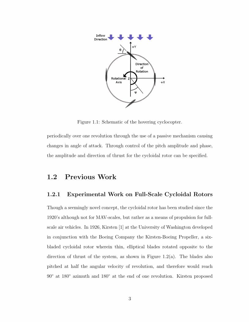
Figure 1.1: Schematic of the hovering cyclocopter.

periodically over one revolution through the use of a passive mechanism causing

changes in angle of attack. Through control of the pitch amplitude and phase,

the amplitude and direction of thrust for the cycloidal rotor can be specified.

1.2 Previous Work

1.2.1 Experimental Work on Full-Scale Cycloidal Rotors

Though a seemingly novel concept, the cycloidal rotor has been studied since the

1920’s although not for MAV-scales, but rather as a means of propulsion for full-

scale air vehicles. In 1926, Kirsten [1] at the University of Washington developed

in conjunction with the Boeing Company the Kirsten-Boeing Propeller, a six-

bladed cycloidal rotor wherein thin, elliptical blades rotated opposite to the

direction of thrust of the system, as shown in Figure 1.2(a). The blades also

pitched at half the angular velocity of revolution, and therefore would reach

90◦ at 180◦ azimuth and 180◦ at the end of one revolution. Kirsten proposed

3

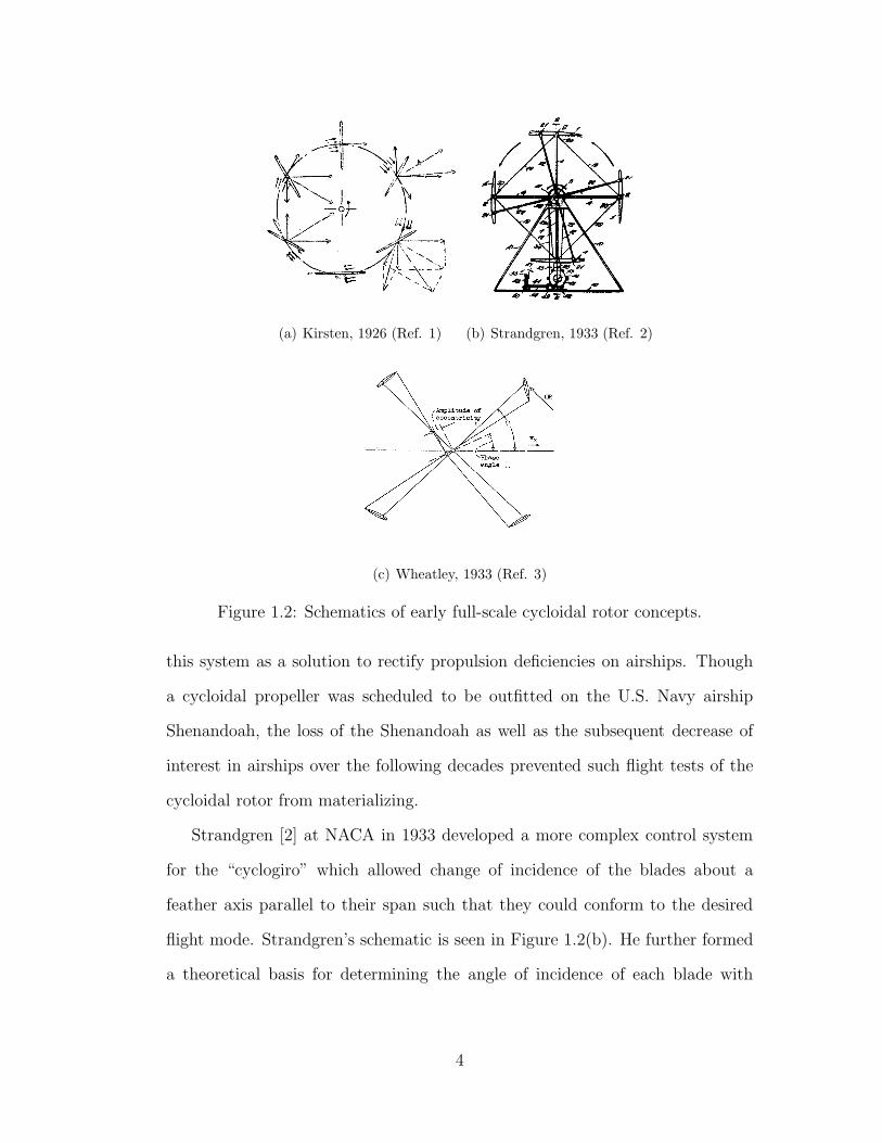
(a) Kirsten, 1926 (Ref. 1) (b) Strandgren, 1933 (Ref. 2)

(c) Wheatley, 1933 (Ref. 3)

Figure 1.2: Schematics of early full-scale cycloidal rotor concepts.

this system as a solution to rectify propulsion deficiencies on airships. Though

a cycloidal propeller was scheduled to be outfitted on the U.S. Navy airship

Shenandoah, the loss of the Shenandoah as well as the subsequent decrease of

interest in airships over the following decades prevented such flight tests of the

cycloidal rotor from materializing.

Strandgren [2] at NACA in 1933 developed a more complex control system

for the “cyclogiro” which allowed change of incidence of the blades about a

feather axis parallel to their span such that they could conform to the desired

flight mode. Strandgren’s schematic is seen in Figure 1.2(b). He further formed

a theoretical basis for determining the angle of incidence of each blade with

4

respect to the freestream, as well as a simple analytical model to evaluate the

resultant forces on the blades.

Concurrently, Wheatley [3] at NACA used a double-cam arrangement on a

cyclogiro to periodically vary both blade amplitude and phase angle, as shown

in Figure 1.2(c). He additionally formed an aerodynamic model for rotor per-

formance based on Momentum Theory with the assumption that the induced

velocities were constant in magnitude throughout the rotor center. By vary-

ing parameters such as solidity and blade aspect ratio, he was able to refine

his design to a more optimized configuration. However, subsequent wind tun-

nel tests in 1935 by Wheatley and Windler [4] for an 8-foot span and diameter

model showed that their simplified theory, while capturing the correct periodic

variation of power, severely underpredicted the zero-lift power due to their low

profile drag coefficient prediction. Hence, they deduced that the cyclogiro would

in forward flight consume an inordinate amount of power, impractical for the

powerplants of the day.

The bulk of the work undertaken in this era showed that the cycloidal rotor

concept was not very feasible at this scale. The problem, as characterized in the

literature, was threefold: a large zero-lift power due to the profile drag from spin-

ning the blades at high incident angles; a large centrifugal force associated with

rotor revolution, from which mechanical problems arose in providing anti-torque

and damping vibrations; and difficulties characterizing the complex, unsteady

flow environment to understand the aerodynamics and predict performance.

5

1.2.2 Interim work on Cycloidal Wind Turbines

After the loss of interest in cycloidal propellers in the early half of the 20th cen-

tury, subsequent research into full-scale cycloidal rotors was commenced by the

wind turbine community. Cycloidal Wind Turbines (CWT), otherwise known

as H-rotors or Giromills, were developed as a new variant of the Vertical Axis

Wind Turbine (VAWT) design. Essentially, a CWT consists of a cycloidal ro-

tor mounted to a mast with blades pitching and rotating perpendicular to the

ground. A straight-bladed VAWT (often abbreviated H-Darrieus, S-VAWT or

SW-VAWT) is essentially a CWT with fixed blade pitch. Since the objective

of a wind turbine is to operate in an effective axial descent condition and ex-

tract drag power from the freestream wind, large profile drag of the blades is a

desirable characteristic, unlike with the cycloidal propeller.

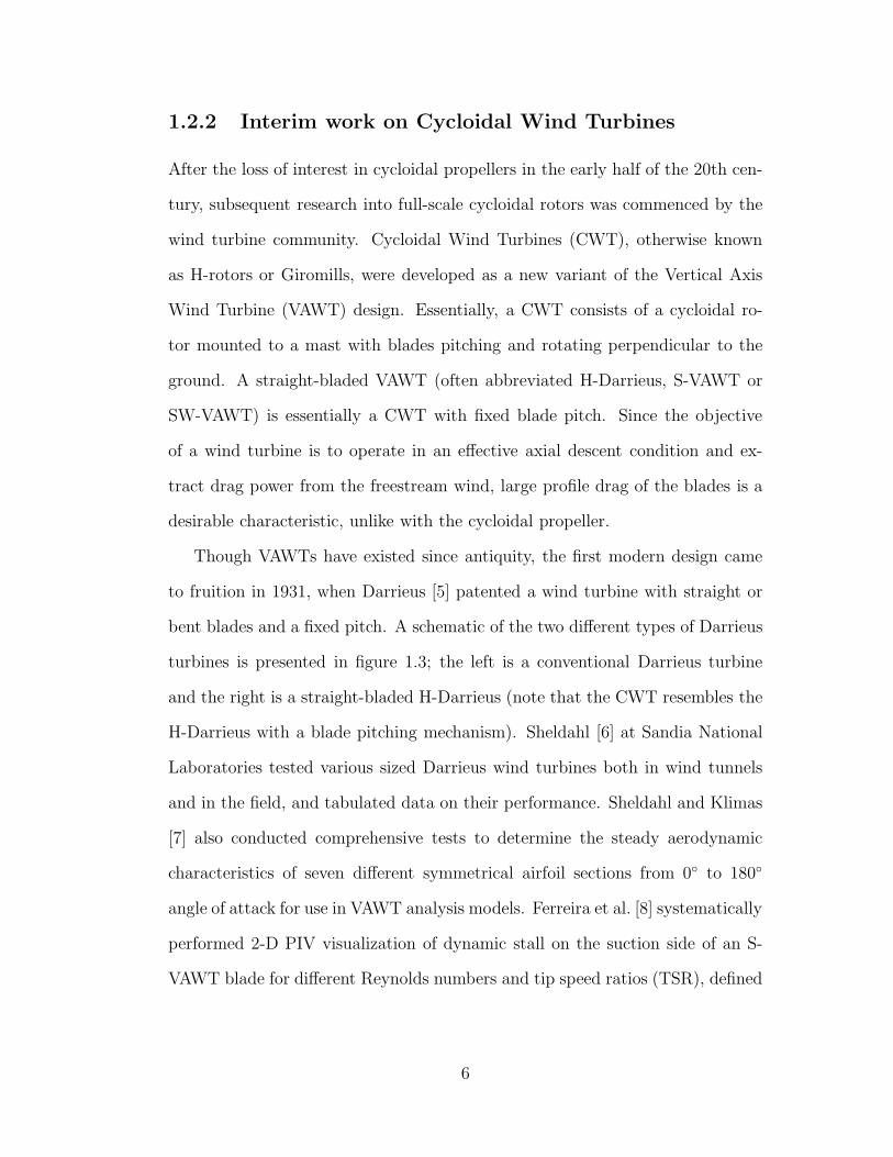
Though VAWTs have existed since antiquity, the first modern design came

to fruition in 1931, when Darrieus [5] patented a wind turbine with straight or

bent blades and a fixed pitch. A schematic of the two different types of Darrieus

turbines is presented in figure 1.3; the left is a conventional Darrieus turbine

and the right is a straight-bladed H-Darrieus (note that the CWT resembles the

H-Darrieus with a blade pitching mechanism). Sheldahl [6] at Sandia National

Laboratories tested various sized Darrieus wind turbines both in wind tunnels

and in the field, and tabulated data on their performance. Sheldahl and Klimas

[7] also conducted comprehensive tests to determine the steady aerodynamic

characteristics of seven different symmetrical airfoil sections from 0◦ to 180◦

angle of attack for use in VAWT analysis models. Ferreira et al. [8] systematically

performed 2-D PIV visualization of dynamic stall on the suction side of an S-

VAWT blade for different Reynolds numbers and tip speed ratios (TSR), defined

6

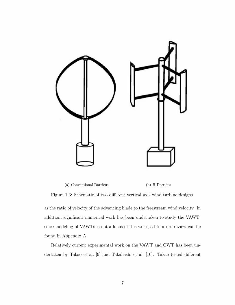
(a) Conventional Darrieus (b) H-Darrieus

Figure 1.3: Schematic of two different vertical axis wind turbine designs.

as the ratio of velocity of the advancing blade to the freestream wind velocity. In

addition, significant numerical work has been undertaken to study the VAWT;

since modeling of VAWTs is not a focus of this work, a literature review can be

found in Appendix A.

Relatively current experimental work on the VAWT and CWT has been un-

dertaken by Takao et al. [9] and Takahashi et al. [10]. Takao tested different

7

configurations for a directed guide vane row in a wind tunnel to improve per-

formance of an S-VAWT. Takahashi tried various NACA 00-series airfoils and

constructed a “wind-lens” structure upstream which collected and accelerated

the flow through the S-VAWT to enhance its performance. Both studies found

that with regard specifically to the VAWT, at low tip speed ratios the VAWT

performed better with increasing TSR due to the blades extracting power at

every section of the rotor, but with higher TSR performance degraded quickly

because portions of the rotor began consuming, instead of extracting power.

With regard to the CWT, Kiwata et al. [11] investigated the effects of using a

four-bar linkage mechanism to passively pitch the blades of an S-VAWT, and

tabulated the performance changes with variations in pitch amplitude, phase

angle, number of blades, and airfoil profiles. He found from his experiments that

cambered blades with almost no phasing generated the maximum power.

1.2.3 Experimental Work on MAV-Scale Cycloidal Ro-

tors

Recently, interest has arisen in applying the cycloidal rotor to MAVs. Though

mechanics and control problems have largely been unresolved, and a good un-

derstanding of the aerodynamics is still lacking, the reduced centrifugal force at

these scales may present a large advantage when compared to full-scale. Also,

the possibility to instantaneously change the direction of thrust using a cycloidal

rotor allows extreme maneuverability, which is useful for MAVs that operate in-

doors and in closed space environments. Furthermore, the cycloidal concept is

very stable in cross-winds and gusts, a problem that plagues many current-day

MAVs.

8

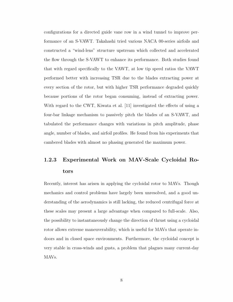
Figure 1.4: The cyclocopter MAV developed by Benedict et al. (Ref. 15)

Previous work on micro-scale aerodynamics of the cycloidal rotor was under-

taken by Hwang et al. [12], who designed and subsequently conducted multidis-

ciplinary optimization of a cyclocopter system, resulting in the construction of

a successfully-hovering micro-scale four-rotor testbed. They demonstrated that

their experimental cyclocopter configuration would produce adequate thrust for

both hover, low-speed forward and maneuvering flight conditions.

Yu et al. [13] experimentally tested the parameters of airfoil geometry, taper

ratio, and control link length on the hovering cyclocopter. As a metric to evaluate

the performance of different cycloidal propeller configurations, they compared

power loading vs. disk loading curves to determine which design produced the

most thrust per unit power for a given disk area. Yu found that to maximize

performance at low Reynolds numbers typical of MAV-scale craft, a flat plate

with minimal taper and slightly higher pitch at the bottom rather than the top

of the cyclocopter cage is desired. The reasoning behind the last design choice

will be discussed in detail later.

A considerable amount of experimental work has been done at the University

of Maryland regarding MAV-scale cycloidal rotors. Benedict et al. [14, 15] as-

9

sembled an experimental model by which he could measure the performance and

examine the flowfield of the cycloidal rotor systematically for various numbers of

blades and rotational speeds. The MAV-scale cyclocopter developed from this

work is shown in Figure 1.4. The weight of the vehicle is ∼ 800g and the length

is ∼ 24in., though the characteristic lengths of blade span and rotor diameter

are both ∼ 6in., thus satisfying the definition of an MAV. Recently, Benedict et

al. [16] investigated the effects of pitching axis location, asymmetric blade pitch

amplitude, airfoil profile, number of blades, and blade flexibility on his cyclo-

copter design; by finding the optimized values of these parameters, he achieved

a large increase in overall efficiency. Overall, these experimental studies have

shown the viability of the cycloidal rotor as a competitive design to conventional

rotors for use on MAVs.

1.2.4 Analytical Models of MAV-Scale Cycloidal Rotors

In addition to experiment, simple analytical studies have been conducted in

literature to predict performance as well as improve design of the cycloidal rotor.

Yun et al. [17] used blade element momentum theory to form a simple algebraic

model for estimation of thrust and inflow produced at the top and bottom half

of the rotor.

McNabb [18] used the equations of Garrick [19] regarding the unsteady lift

and moments of a 2-D airfoil moving in sinusoidal motion and derived equations

for simplified unsteady aerodynamics of a cycloidal rotor with realistic four-

bar blade pitching motion, both in hover and forward flight. He also modeled

the downwash as a constant velocity flow through the rotor because the effect of

induced angle of attack on the bottom blade could not be neglected, but relegated

10

interactions between the blades to first-order analysis. From this, he found

that his model could predict to within 10% accuracy the power and total force

obtained from the Wheatley wind tunnel tests. In addition, McNabb deduced

that the aerodynamic loads were insignificant compared to the inertial loads;

and, though susceptible to wind gusts, the resultant force on the cyclocopter

was quickly damped out.

Parsons [20] used double-multiple streamtube theory to analyze flow through

the cycloidal rotor. In this analysis, “multiple” denotes that the flow through

the rotor is subdivided into a number of streamtubes; these streamtubes are

aerodynamically independent of each other and have different induced velocities

at the upstream and downstream halves of the volume swept by the rotor. For

each streamtube, “double” indicates that the rotor is modeled as two thin actu-

ator disks such that the effects of the upstream wake on the downstream blades

are captured. The flow through the rotor was assumed to be one-dimensional,

incompressible and inviscid. Solving for the conservation equations, Parsons was

able to obtain a relatively accurate first-order model to estimate the aerodynamic

forces and power of his cycloidal rotor setup.

More recently, Benedict et al. [21] developed an analytical model to predict

the performance of their MAV-scale rotor at different symmetric and asymmetric

pitching angles, pitch link locations, and rotational speeds. From their results,

they found that the thrust prediction correlated well with experiment, but there

were discrepancies in power prediction. Though Benedict’s and other lower order

models described above can predict the performance fairly reasonably, they do

not provide much insight into the underlying flow physics.

11

1.2.5 CFD Studies of MAV-Scale Cycloidal Rotors

CFD can provide a better understanding of the flow physics in the complex cy-

cloidal rotor environment. However, CFD needs to carefully validated against

experiments to ensure accuracy of the results. Previously, Hwang et al. con-

ducted both a 2-D and 3-D analysis using STAR-CD (a commercially available

CFD solver) with a k-ε turbulence model on a micro scale four-bladed cycloidal

rotor. The analysis was run on an unstructured mesh generated with the Pa-

tran Command Language, with blade pitching simulated using the moving mesh

method. From this, they determined the optimal conditions by which their cy-

clocopter design operated and calculated a power requirement within 15% of the

experimental value. However, though their 3-D analysis predicted performance

correctly, it utilized relatively coarse meshes and therefore, could not provide

much insight into the flowfield. In addition, the use of the high-Reynolds k-ε

turbulence model for such a low-Reynolds application may not have been appro-

priate.

Iosilevskii and Levy [22] studied both two- and four-bladed cyclocopters using

the 2-D EZNSS flow solver assuming laminar compressible flow, with time inte-

gration conducted using the implicit Beam-Warming algorithm. Their code was

run at low Reynolds and Mach numbers with a micro-scale characteristic chord

length, comparable aspect ratio and rotor radius-to-chord ratio to Benedict’s

work, and pitch angles of 15◦ - 25◦. The blades were simulated with body-fitted

C-shaped meshes, then overset with a Chimera scheme on a Cartesian back-

ground mesh. From this analysis, they demonstrated that the effectiveness of

a cycloidal rotor may be comparable with that of a heavy-loaded helicopter ro-

tor. However, their 2-D simulation assumed infinite span and therefore, did not

12

capture the complete 3-D flow physics. Furthermore, their use of a relatively

coarse Cartesian background mesh also lacked the grid refinement to accurately

visualize the flow.

1.3 Objective of Current Work

The current work focuses on developing and validating a CFD based methodol-

ogy that can help understand the aerodynamics of the cyclocopter and details

of the flow physics which was missing in previous works. This entails modify-

ing an existing Reynolds Averaged Navier-Stokes (RANS) compressible solver,

previously employed by Lakshminarayan and Baeder [23] in the aerodynamic

investigation of micro-scale hovering coaxial rotors, to be applicable to cycloidal

rotor geometries. The primary objective is to characterize unsteady performance

and provide insight into the flow physics. The secondary objective is to refine

the solver to obtain force and power values comparable to MAV-scale cycloidal

rotor experiments, thus becoming an accurate predictive tool for performance.

A tertiary objective is to apply the understanding of the flow physics obtained

from this work to improve rotor design. Due to the difficulty of simulating such

a dynamic flow environment, numerical simulation of cycloidal rotors has not

been previously studied to a great extent. It is hoped that through this work,

the improved predictive capability of the current CFD solver will provide a pow-

erful tool to understand flow physics and benefit future optimization efforts for

this rotor configuration.

13

1.4 Thesis Outline

This thesis is organized into six chapters. Chapter one provides the definition

of the problem, previous experimental and numerical work, and the objective

of the current research. Chapter two describes details on grid generation, pre-

scribed grid motions and deformations, and specific numerical methods used

in the flow solver. Preliminary tests on steady symmetric airfoils and unsteady

pitching airfoils that were performed to validate the solver are presented in chap-

ter three, thus allowing confidence to be gained in the accuracy of the flow so-

lution. In Chapter four, the experimental setup of Benedict et al. used for

validation of the flow solver on cycloidal rotor geometries is described. Also, it

describes cyclocopter-specific overset grid generation, deformations, and blade

motion incorporated into the flow solver to provide a high fidelity simulation of

the experiment. In addition, Chapter four compares performance of both the

2-D and 3-D CFD solvers to the experiment, and exhibits the strengths as well

as shortcomings of both solvers in predicting the thrust and aerodynamic power

of the cycloidal rotor at various operational conditions. Chapter five provides

insight into the flowfield as predicted by the 3-D flow solver. In particular, it

explores the unsteady performance and three-dimensionality of the flowfield in

ways difficult to achieve with experimentation. Finally, a summary of results

from the present study as well as future work for improving the quality of the

CFD predictions for the cyclocopter is proposed in chapter six.

14

1.5 Key Contributions of the Current Work

As will be presented in the following chapters, the current work provides sev-

eral key contributions to simulating and understanding of the cyclocopter and

its flow physics. Firstly, the simulation incorporated a high-resolution overset

mesh system with a realistic “four-bar” grid motion and blade deformations to

achieve a highly-detailed model of the experiment. This grid was specifically

targeted to resolve the flow physics; this was unprecedented in previous works,

which only focused on design. Secondly, it validated the current flow solver with

experiments at low-Reynolds flows of interest with large unsteady blade motions

at high angles of attack. This reinforced the confidence in the solver to predict

accurate results in highly unsteady and separated flows. Thirdly, it compared

the flow solver with cyclocopter experiments and noted its predictive capability

for both force and power. It also sought to explain the cause for discrepancies

between CFD and experiment, and suggested future improvements to the simu-

lation for improvement of accuracy. Finally, this work provided unprecedented

insight in understanding the three-dimensionality of the cyclocopter flowfield as

well as provided highly detailed flow visualization. It associated specific observed

flow phenomena with the trends seen in performance, thus allowing greater ad-

vancement in the understanding of the cycloidal rotor aerodynamics.

15

Chapter 2

Methodology

Computational Fluid Dynamics (CFD) is a powerful tool to provide flow visual-

ization and performance predictions of low-Reynolds number flight regimes. It

can allow for insight into the flowfield in ways unattainable or impractical with

experiment, as well as provide an inexpensive way for testing new blade designs

and rotor configurations to arrive at an optimized design. However, all CFD

solvers must be first validated with a baseline experiment to ensure physical

results are being produced.

For all CFD approaches, a mesh must first be generated that resolves the ge-

ometry, as well as provides sufficient resolution to capture flow features without

smearing. Secondly, the governing equations must be chosen such that they are

adequate for the flow regime of interest, especially taking into consideration the

Reynolds and Mach numbers at which the vehicle operates. Boundary conditions

must also be imposed on the geometric surfaces as well as the farfield. Finally,

the numerical solver methodologies must be chosen such they they can itera-

tively solve the governing equations to arrive at a solution which closely matches

experiment. This chapter will describe such numerical methodologies with spe-

cific focus on those used in the Overset Transonic Unsteady Rotor Navier-Stokes

16

(OVERTURNS) code [24], the flow solver employed in this work.

2.1 Grid Generation Methods

A well-generated mesh which has sufficient resolution to capture essential flow

structures such as tip vortices, while not being too computationally expensive

to solve, is crucial for a reliable CFD model. The cycloidal rotor simulation

utilized body-fitted C-O blade meshes which were overset onto cylindrical back-

ground meshes. On the blade mesh, the airfoil surface is modeled as a viscous,

adiabatic wall. The mesh extending from this blade surface contains points in

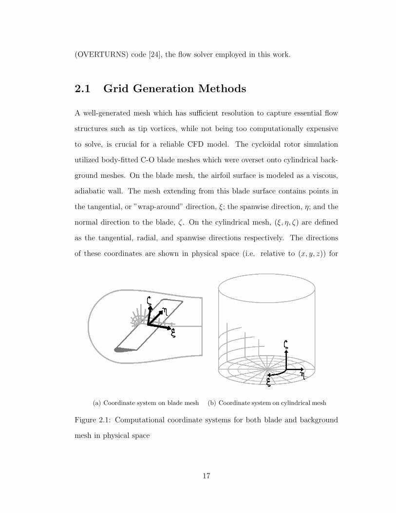
the tangential, or ”wrap-around” direction, ξ; the spanwise direction, η; and the

normal direction to the blade, ζ . On the cylindrical mesh, (ξ, η, ζ) are defined

as the tangential, radial, and spanwise directions respectively. The directions

of these coordinates are shown in physical space (i.e. relative to (x, y, z)) for

(a) Coordinate system on blade mesh (b) Coordinate system on cylindrical mesh

Figure 2.1: Computational coordinate systems for both blade and background

mesh in physical space

17

both meshes in Figure 2.1. A simple grid transformation from physical space to

computational space is used to account for geometric changes and stretching fac-

tors used in physical space; one can think of this as “unwrapping” the grid from

the airfoil or the background mesh and mapping it onto a Cartesian coordinate

system. This process is computationally inexpensive and maintains accuracy;

the resultant Cartesian computational grid allows the governing equations to be

solved.

For the cyclocopter grids, an algebraic grid generation scheme was employed

for the background meshes and a hyperbolic grid generator was used to produce

the blade meshes. The following subsections will provide a brief overview of each

grid generation methodology.

2.1.1 Algebraic Grid Generation

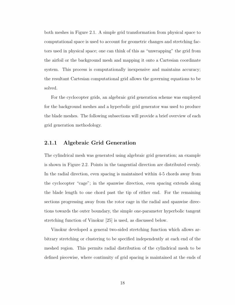
The cylindrical mesh was generated using algebraic grid generation; an example

is shown in Figure 2.2. Points in the tangential direction are distributed evenly.

In the radial direction, even spacing is maintained within 4-5 chords away from

the cyclocopter “cage”; in the spanwise direction, even spacing extends along

the blade length to one chord past the tip of either end. For the remaining

sections progressing away from the rotor cage in the radial and spanwise direc-

tions towards the outer boundary, the simple one-parameter hyperbolic tangent

stretching function of Vinokur [25] is used, as discussed below.

Vinokur developed a general two-sided stretching function which allows ar-

bitrary stretching or clustering to be specified independently at each end of the

meshed region. This permits radial distribution of the cylindrical mesh to be

defined piecewise, where continuity of grid spacing is maintained at the ends of

18

each adjacent piecewise segment.

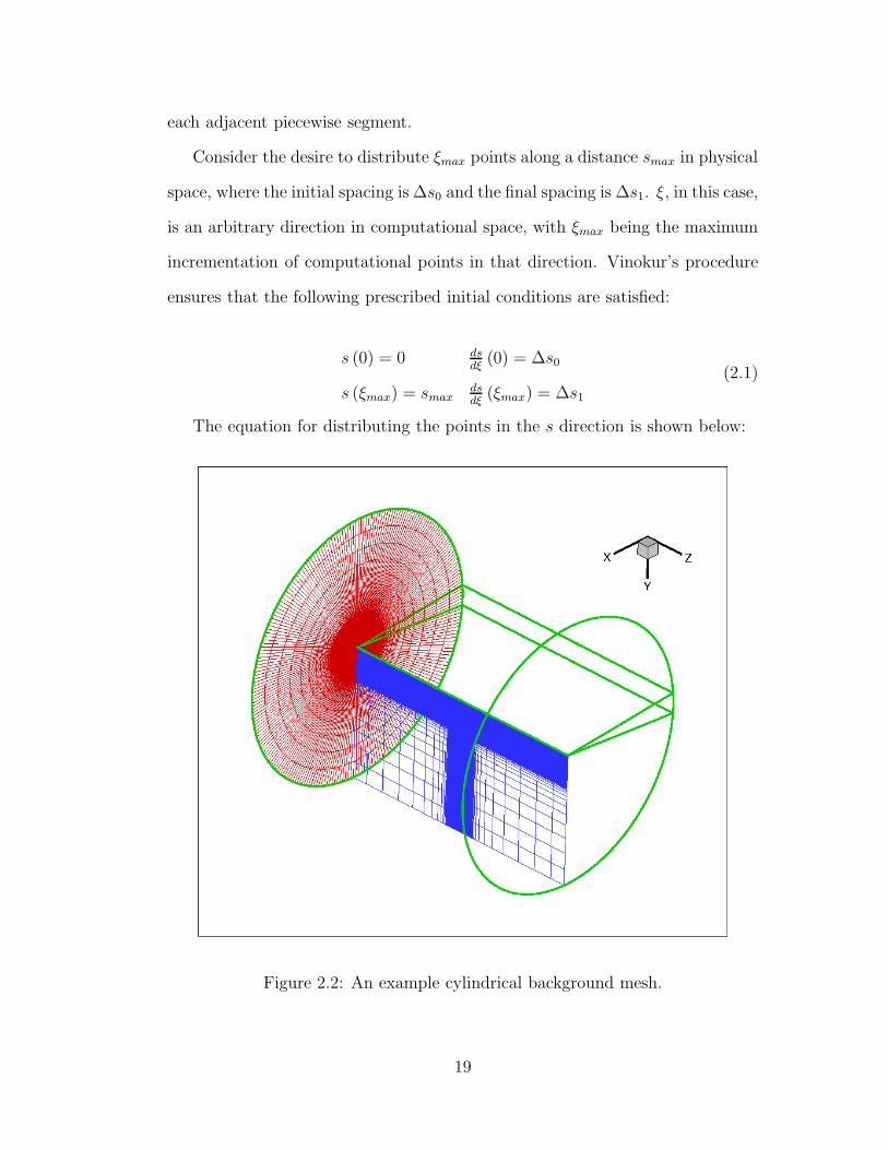
Consider the desire to distribute ξmax points along a distance smax in physical

space, where the initial spacing is ∆s0 and the final spacing is ∆s1. ξ, in this case,

is an arbitrary direction in computational space, with ξmax being the maximum

incrementation of computational points in that direction. Vinokur’s procedure

ensures that the following prescribed initial conditions are satisfied:

s (0) = 0 dsdξ

(0) = ∆s0

s (ξmax) = smaxdsdξ

(ξmax) = ∆s1

(2.1)

The equation for distributing the points in the s direction is shown below:

Figure 2.2: An example cylindrical background mesh.

19

s (ξ) =uV (ξ)

AV + (1 − AV ) uV (ξ)(2.2)

where

AV =

√∆s0√∆s1

(2.3)

uV (ξ) =1

2+

tan [∆z (ξ − 1/2)]

2 tan (∆z/2)(2.4)

sin ∆z

∆z=

1

ξmax

√∆s0∆s1

(2.5)

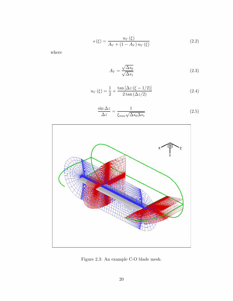
Figure 2.3: An example C-O blade mesh.

20

In the above equations, AV is a constant based on a given ∆s0 and ∆s1. ∆z

is the recursive solution of the transcendental equation Eq. 2.5 and thus is a

function of the desired end grid spacings as well as the total number of points to

be distributed. When the above series of equations are solved, s (ξ) will describe

the distribution of points along a line in physical space as a function of the

incrementation in an arbitrary direction of computational space, ξ.

2.1.2 Hyperbolic Grid Generation

Hyperbolic mesh generation was used to create the blade mesh. This type of

mesh generation allows a high-quality mesh that maintains orthogonality to be

generated from an initial specification of cell size, distance, and surface data. It

ensures that the cells close to the surface do not suffer from distortion, as well as

allows the transformation of partial differential equations to produce the smallest

number of additional terms while retaining the greatest accuracy for numerical

differencing techniques [26]. Using these methods, good resolution at the airfoil

surface and areas of interest, as well as good cell sizing, are maintained. Further,

“local” problems can be avoided such as propagation of initial discontinuities

and the formation of grid shocks, thus easing the implementation of turbulence

models [27] and increasing computational efficiency.

In the application of a hyperbolic scheme, the mesh is propagated in the nor-

mal direction (essentially time-like) from an initial boundary curve (essentially

space-like), where each new state is generated from the known conditions at the

current state. For the cycloidal rotor blades, these planes are continually ex-

truded from the blade surface until a predefined boundary limit. An example C-

O blade mesh is shown in Figure 2.3. More detail on two-dimensional hyperbolic

21

grid generation can be found in works by Alsalihi [28], Cordova and Barth [29],

and Kinsey and Barth [30] ; a generalized method for three-dimensional hyper-

bolic generation is described by Chan and Steger [31].

For an isolated blade mesh, the hyperbolic generation is allowed to extrude

out to at least 20 chords away from the blade surface. However, for a blade

overset onto a background mesh, the blade mesh region only extends to at most

2 chords away from the blade surface to avoid overlap in multi-bladed cases.

2.2 Overset Grid Methodology

As discussed in the previous sections, finely-spaced blade meshes are overset

onto a coarser background mesh to allow for blade motion and maintain compu-

tational efficiency while capturing all of the flow features. An example overset

blade/background mesh system for a hypothetical 2-bladed cycloidal rotor with

40◦ initial blade pitch is shown in Figure 2.4. In this system, information is

(a) Chordwise view (b) Spanwise view

Figure 2.4: Example overset blade / background mesh system for a 2-bladed

cycloidal rotor with 40◦ initial pitch.

22

transferred between these two meshes through domain connectivity. In this pro-

cess, a “donor” cell on one mesh will give information to a “receiver” cell on

the other mesh. Significant effort is made to ensure that the donor and receiver

cells are roughly equivalent in size, such that information can be interpolated

between meshes without loss of too much accuracy. In addition, a “hole” is cut

in the background mesh where the blade mesh is located to maintain consistency

of solution in the entire computational domain.

In this work, the Implicit Hole-Cutting (IHC) routine developed by Lee and

Baeder [32] and refined by Lakshminarayan [24] was used to determine the con-

nectivity information between the blade and background meshes. Lee and Baeder

refined the baseline Chimera hole-cutting technique in OVERTURNS, which was

capable of handling only two overset meshes. The original overset routine in-

volved specifying a box around the blade and extracting a list of hole fringe

points that require information from other grids to serve as boundary condi-

tions. To avoid the effect of invalid hole points on the solution, an array of

integers (the iblank array) is defined, one for each grid point, with the value

0 for hole and fringe points, and 1 for field points. However, defining such an

arbitrary box around the body with the iblank array forces the hole to be cut in

the same location regardless of differences in grid resolution between the blade

and background meshes. Therefore, a large difference in grid resolution could

result in hole fringe points interpolating from donors that have extremely differ-

ent cell volumes from receivers, resulting in a high level of inaccuracies with the

interpolation.

Lee and Baeder’s approach used an intermediate background mesh to improve

transfer of information from the blade mesh to the background mesh, and could

23

be operated without prior knowledge of where the hole fringe points are. At

every point in the grid, the IHC method computes the solution on the cells

having the smallest volume, then selects these “best quality” cells in multiple

overlapped regions to interpolate to other points, leaving the rest as hole points.

Lakshminarayan improved on the work of Lee and Baeder by implementing

an iblank array to the IHC routine. The original IHC routine required thick

hole fringe layers to completely enclose the body to prevent invalid points, but

this required a large number of interpolations, and furthermore sufficiently thick

fringe layers were not always guaranteed. The Lakshminarayan approach allowed

blanking of the hole fringe points during implicit inversion, thus permitting the

use of valid solutions from the blanked out points in the flux calculations by

setting iblank to −1. Hence, Lakshminarayan’s method makes Lee’s hole-cutting

process less computationally intensive while still maintaining accuracy.

2.3 Grid Motion

An accurate simulation of the cycloidal rotor as consistent with experiment re-

quires that the blade rotation and pitching about the rotor cage be prescribed

as a blade grid motion on the background mesh. In addition, the structural

deformations due to centrifugal forces from spinning at a high RPM must be

prescribed onto the blade mesh as well. The following subsections explore the

numerical procedures for incorporating such grid motions into the flow solver.

24

2.3.1 Grid Rotation

For each physical timestep taken in the flow solver, the blade meshes are rotated

azimuthally about the rotor center. The non-dimensional timestep size, ∆t, as

determined in Table 2.1, is equivalent to the incremental degree of azimuth that

the blade meshes are rotated. For example, if non-dimensional ∆t was set to

0.25, the blade meshes would move a quarter-degree per iteration. Hence, with

this example timestep size, 1440 iterations would correspond to one revolution

about the rotor cage.

2.3.2 Numerical Approximation of the Four-Bar Pitching

Mechanism

To provide a high-fidelity model of the blade pitch for the flow solver, a numer-

ical approximation was used to prescribe this motion to the blade meshes. The

experimental cyclocopter employed a pitching mechanism developed by Parsons

and refined by Benedict to passively pitch the blades. This mechanism con-

sists of two pitch bearings, arranged such that they cause an offset between the

axis of the rotor shaft and an offset ring; Benedict denotes this distance as L2.

This configuration essentially comprises a crank-rocker type four-bar pitching

mechanism, with the offset distance L2 determining the pitch amplitude. Al-

though this configuration ideally approximates a sinusoidal motion, mechanical

limitations result in a pitching motion with about 10◦ phase offset from a truly

sinusoidal curve. Figure 2.5 shows the variation in pitch angle over one rotor

revolution with the four-bar mechanism as a function of azimuthal angle, as

compared with a pure sinusoidal pitch angle variation, for 35◦ pitch amplitude.

As seen from the figure, the blades achieve a maximum pitch angle in the the

25

Figure 2.5: Pitch variation with respect to azimuthal angle for the four-bar

linkage mechanism.

positive y-direction (with respect to the axis in Figure 1.1) when slightly past

the Ψ = 0◦ and Ψ = 180◦ azimuthal positions i.e. the “bottom” and “top” of

the rotor cage. The “collective pitch amplitude” described hereafter refers to the

maximum pitch angle which the blade attains at these two azimuthal locations.

At a slight offset past Ψ = 90◦ and Ψ = 270◦, which correspond to the “sides”

of the cyclocopter cage, the pitch angle goes to zero.

In the flow solver, blade pitch is calculated using numerical approximation

to the aforementioned four-bar linkage mechanism, shown below.

θ = π/2 + 2 tan−1 Ψ1 (2.6)

where

Ψ1 =sin Ψ −

√

sin2 Ψ + (cos Ψ + L1/L2)2 + f 2

cos Ψ + L1/L2 + f(2.7)

26

f =L1

L4

cos Ψ +L2

1 + L22 + L2

4 − L23

2L2L4

(2.8)

In the above equations, L1, L2, L3, and L4 represent the non-dimensional

lengths of pitch linkages with respect to the blade chord, and determine the

pitching motion. θ denotes pitch amplitude and Ψ is azimuthal angle of the

blade around the rotor cage. Details regarding the application of this equation

to the cyclocopter are provided in Section 4.3.

2.3.3 Blade Deformations

From a structural dynamic perspective, a blade dynamic response distribution

can be prescribed onto the numerical grids to ensure accuracy and consistency

with experiment. The methodology provided by Sitaraman [33] was modified

such that it was applicable to the cycloidal rotor geometry.

A structural dynamic analysis developed by Benedict et al. [21] was used to

output blade deformations. Benedict developed an FEM-based aeroelastic anal-

ysis by modeling the cycloidal rotor blades as second-order non-linear, isotropic

Euler-Bernoulli beams with six spanwise elements undergoing radial bending,

tangential bending, and elastic twist (torsion, φ) deformations, as shown in Fig-

ure 2.6. This was based on the coupled flap-lag-torsion equations of Hodges

and Dowell [34]. The blades were assumed to have pin-pin boundary conditions

on both ends for bending and fixed-free boundary conditions for torsion due to

the rigid pitch link on the root end. In addition, Hamilton’s principle was used

to develop the equations of motion for the blade. The finite element in time

method was used with 60 timewise elements to obtain the steady blade periodic

response.

27

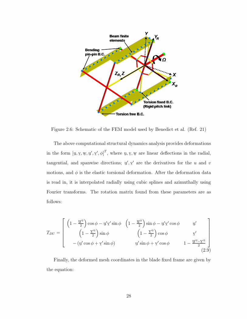
Figure 2.6: Schematic of the FEM model used by Benedict et al. (Ref. 21)

The above computational structural dynamics analysis provides deformations

in the form [u¯, v¯, w¯, u¯′, v

¯′, φ]T , where u

¯, v¯, w¯

are linear deflections in the radial,

tangential, and spanwise directions; u¯′, v

¯′ are the derivatives for the u and v

motions, and φ is the elastic torsional deformation. After the deformation data

is read in, it is interpolated radially using cubic splines and azimuthally using

Fourier transforms. The rotation matrix found from these parameters are as

follows:

TDU =

(

1 − u¯

′2

2

)

cos φ − u¯′v¯′ sin φ

(

1 − u¯

′2

2

)

sin φ − u¯′v¯′ cos φ u

¯′

(

1 − v¯

′2

2

)

sin φ(

1 − v¯

′2

2

)

cos φ v¯′

− (u¯′ cos φ + v

¯′ sin φ) u

¯′ sin φ + v

¯′ cos φ 1 − u

¯′2−v

¯′2

2

(2.9)

Finally, the deformed mesh coordinates in the blade fixed frame are given by

the equation:

28

x′

y′

z′

= (T ′

DU)T

x

y

z

+

u¯

v¯

w¯

(2.10)

2.4 Flow Solver

With the grid generated and the grid motions prescribed, the initial setup for

the flow solver is completed. The flowfield properties at each grid point within

the overset mesh system can now be obtained by solving the conservation laws

of physics for fluid flow. The following subsections describe these governing

equations, as well as certain numerical methods to ensure their convergence for

low-Mach and Reynolds number flight regimes. This section will conclude with

a description of the specific numerical methods used in the OVERTURNS CFD

code It should be noted that TURNS refers to the baseline flow solver, whereas

OVERTURNS is the overset version of the solver. However, these terms are used

interchangeably in this work.

2.4.1 Compressible Navier-Stokes Equations

The Navier-Stokes equations comprise the mass, momentum, and energy con-

servation governing equations used in the flow solver. These equations solve for

compressibility as well as viscous effects, which are particularly important for

the low-Reynolds numbers flows pertaining to the cyclocopter MAV. The 3-D

compressible Navier-Stokes equations in physical space (i.e. (x, y, z) coordinates)

are given by:

29

∂Q

∂t+

∂E

∂x+

∂F

∂y+

∂G

∂z= S (2.11)

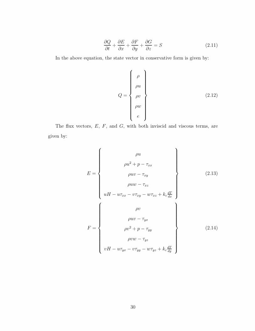
In the above equation, the state vector in conservative form is given by:

Q =

ρ

ρu

ρv

ρw

e

(2.12)

The flux vectors, E, F , and G, with both inviscid and viscous terms, are

given by:

E =

ρu

ρu2 + p − τxx

ρuv − τxy

ρuw − τxz

uH − uτxx − vτxy − wτxz + kcdTdx

(2.13)

F =

ρv

ρuv − τyx

ρv2 + p − τyy

ρvw − τyz

vH − uτyx − vτyy − wτyz + kcdTdy

(2.14)

30

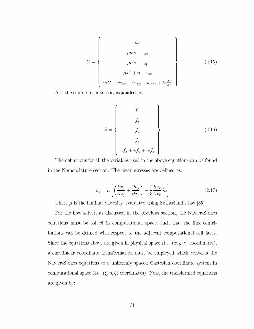
G =

ρw

ρuw − τzx

ρvw − τzy

ρw2 + p − τzz

wH − uτzx − vτzy − wτzz + kcdTdz

(2.15)

S is the source term vector, expanded as:

S =

0

fx

fy

fz

ufx + vfy + wfz

(2.16)

The definitions for all the variables used in the above equations can be found

in the Nomenclature section. The mean stresses are defined as:

τij = µ

[(

∂ui

∂xj

+∂uj

∂xi

)

− 2

3

∂uk

∂xk

δij

]

(2.17)

where µ is the laminar viscosity, evaluated using Sutherland’s law [35].

For the flow solver, as discussed in the previous section, the Navier-Stokes

equations must be solved in computational space, such that the flux contri-

butions can be defined with respect to the adjacent computational cell faces.

Since the equations above are given in physical space (i.e. (x, y, z) coordinates),

a curvilinear coordinate transformation must be employed which converts the

Navier-Stokes equations to a uniformly spaced Cartesian coordinate system in

computational space (i.e. (ξ, η, ζ) coordinates). Now, the transformed equations

are given by:

31

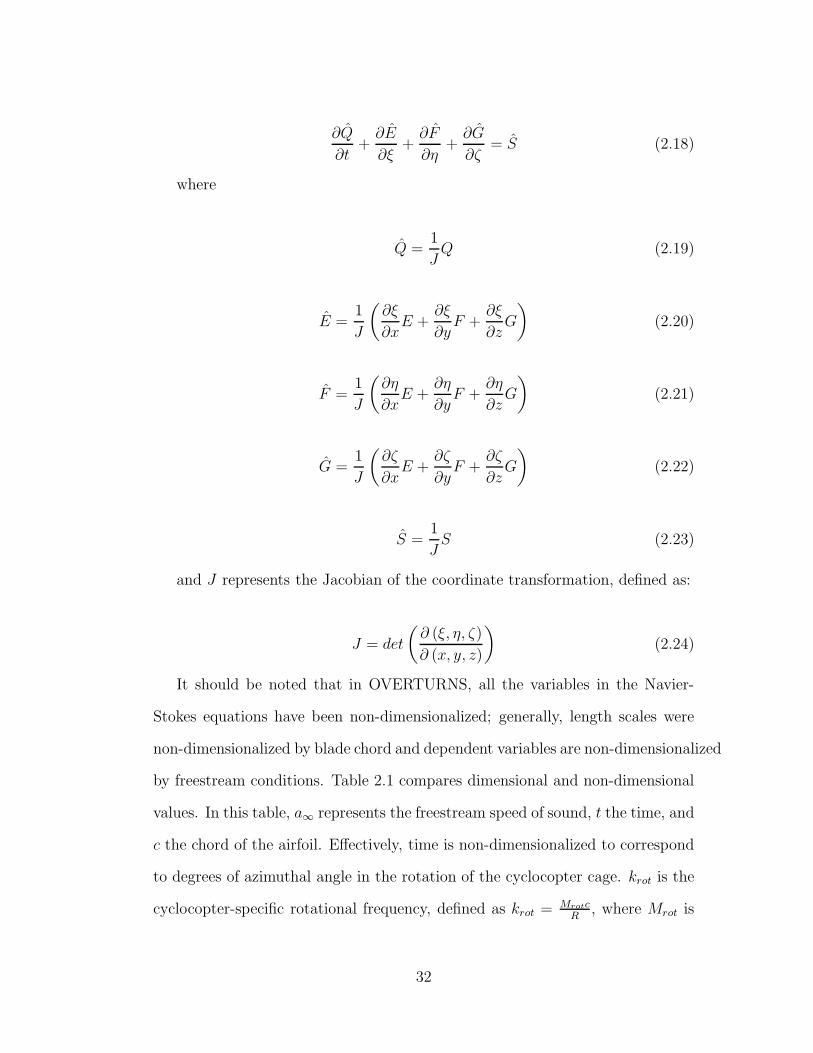
∂Q

∂t+

∂E

∂ξ+

∂F

∂η+

∂G

∂ζ= S (2.18)

where

Q =1

JQ (2.19)

E =1

J

(

∂ξ

∂xE +

∂ξ

∂yF +

∂ξ

∂zG

)

(2.20)

F =1

J

(

∂η

∂xE +

∂η

∂yF +

∂η

∂zG

)

(2.21)

G =1

J

(

∂ζ

∂xE +

∂ζ

∂yF +

∂ζ

∂zG

)

(2.22)

S =1

JS (2.23)

and J represents the Jacobian of the coordinate transformation, defined as:

J = det

(

∂ (ξ, η, ζ)

∂ (x, y, z)

)

(2.24)

It should be noted that in OVERTURNS, all the variables in the Navier-

Stokes equations have been non-dimensionalized; generally, length scales were

non-dimensionalized by blade chord and dependent variables are non-dimensionalized

by freestream conditions. Table 2.1 compares dimensional and non-dimensional

values. In this table, a∞ represents the freestream speed of sound, t the time, and

c the chord of the airfoil. Effectively, time is non-dimensionalized to correspond

to degrees of azimuthal angle in the rotation of the cyclocopter cage. krot is the

cyclocopter-specific rotational frequency, defined as krot = MrotcR

, where Mrot is

32

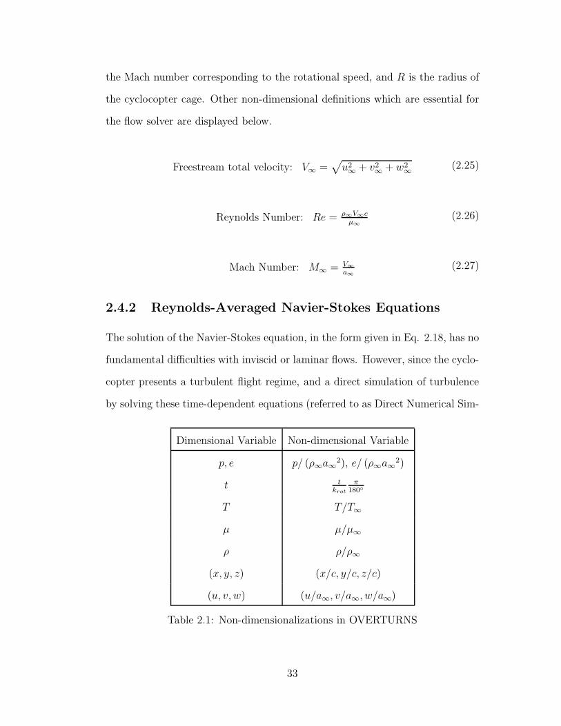
the Mach number corresponding to the rotational speed, and R is the radius of

the cyclocopter cage. Other non-dimensional definitions which are essential for

the flow solver are displayed below.

Freestream total velocity: V∞ =√

u2∞

+ v2∞

+ w2∞

(2.25)

Reynolds Number: Re = ρ∞V∞c

µ∞

(2.26)

Mach Number: M∞ = V∞

a∞

(2.27)

2.4.2 Reynolds-Averaged Navier-Stokes Equations

The solution of the Navier-Stokes equation, in the form given in Eq. 2.18, has no

fundamental difficulties with inviscid or laminar flows. However, since the cyclo-

copter presents a turbulent flight regime, and a direct simulation of turbulence

by solving these time-dependent equations (referred to as Direct Numerical Sim-

Dimensional Variable Non-dimensional Variable

p, e p/ (ρ∞a∞2), e/ (ρ∞a∞

2)

t tkrot

π180◦

T T/T∞

µ µ/µ∞

ρ ρ/ρ∞

(x, y, z) (x/c, y/c, z/c)

(u, v, w) (u/a∞, v/a∞, w/a∞)

Table 2.1: Non-dimensionalizations in OVERTURNS

33

ulation, DNS) is very computationally intensive, an approximation to turbulence

is needed.

For engineering and physics problems, the Reynolds-Averaged Navier-Stokes

(RANS) equations represent an approximation that considerably reduces the

amount of calculations needed to solve the governing equations. The RANS

equations decompose the flow into mean and fluctuating parts, i.e. any flow

variable can be written in the form:

φ = φ + φ′ (2.28)

φ represents the mean part, which is obtained from Reynolds averaging in

the equation:

φ =1

χlim

∆t→∞

1

∆t

∫ ∆t

0

χφ (t) dt (2.29)

where χ = 1 if φ = ρ or φ = p, and χ = ρ for other variables. φ′ is the

fluctuating part of the equation, and its Reynolds average is zero. These decom-

posed parts, when placed in the Navier-Stokes equations (Eq. 2.18), result in

the mathematical description of the mean flow properties. If we drop the bar

on the mean flow variables, the resulting equations are the same as the instan-

taneous Navier-Stokes equations except for additional terms in the momentum

and energy equations; these additional terms are denoted as the Reynolds Stress

Tensor, and account for the additional stress due to turbulence. However, these

additional Reynolds-stress terms are now unknown, and must be approximated

using a turbulence model to achieve closure of the RANS equations.

34

2.4.3 Turbulence Model

The turbulent controibution to viscosity is approximated by the Reynolds Stress

Term, shown below:

τRij = −ρu′

iu′

j (2.30)

Eq. 2.17 showed the Reynolds stresses with the assumption of isotropic eddy

viscosity. Although many turbulence models have been developed to obtain

turbulent viscosity, this thesis will focus solely on the two models that were

used extensively in this work: the Baldwin-Lomax model [36], and the Spalart-

Allmaras model [37].

The Baldwin-Lomax (BL) model is a two-layer algebraic 0-equation model

which uses boundary layer velocity profile to determine eddy viscosity. At its

core, the model uses the equation:

νt =

νtinner, if y ≤ ycrossover

νtouter, if y > ycrossover

(2.31)

where ycrossover is the minimum distance from the surface where νtinner=

νtouter. These are respectively given by:

νtinner= ρ

[

ky

(

1 − e−y+

A+

)]2

∣

∣

∣

∣

∣

∣

√

1

2

(

∂ui

∂xj

− ∂uj

∂xi

)2

∣

∣

∣

∣

∣

∣

(2.32)

νtouter= ρKCCP FWAKEFKLEB (y) (2.33)

Details on the variables found in these equations can be found in [36]. The

Baldwin-Lomax model is suitable for high-speed attached flows with thin bound-

ary layers. Though the BL model is not meant for use with unsteady, separated

35

flows, it can still provide a quick preliminary approach to solving turbulent eddy

viscosity, especially in cases where robustness is more important than capturing

flow physics details.

The Spalart-Allmaras (SA) turbulence model is a one-equation model given

by:

∂ν

∂t+ V · (∇ν) =

1

σ

[

∇ · ((ν + ν)∇ν) + cb2 (∇ν)2]

+ cb1Sν − cw1fw

[ ν

d

]2

(2.34)

The SA model relates the Reynolds stresses to the mean strain. The turbulent

eddy viscosity, νt, is obtained by solving the above PDE for a related variable,

ν, where the two quantities are related by νt = νfv1. fv1 is a function of ν and

the molecular viscosity, ν. cb1, cb2, and cw1 are constants, d is distance from

the wall, and V is the mean flow velocity; further details can be found in [37].

Essentially, after loose coupling of this equation to the Navier-Stokes equations,

the turbulent eddy viscosity can be obtained, from which the shear stress in the

moment and energy equations can be evaluated, thus providing closure for all

the variables.

2.4.4 Spatial Discretization

In OVERTURNS, the baseline algorithm uses a finite volume approach to dis-

cretize Equation 2.18 in space and time; the discrete approximation is shown in

Equation 2.35. In the finite volume approach, a fictitious control volume is cre-

ated around each gridpoint; its boundaries are defined by the midpoints of each

line joining the current gridpoint to its neighboring gridpoints. At these bound-

aries, or “faces”, of the control volume, the fluxes are evaluated, thus allowing

36

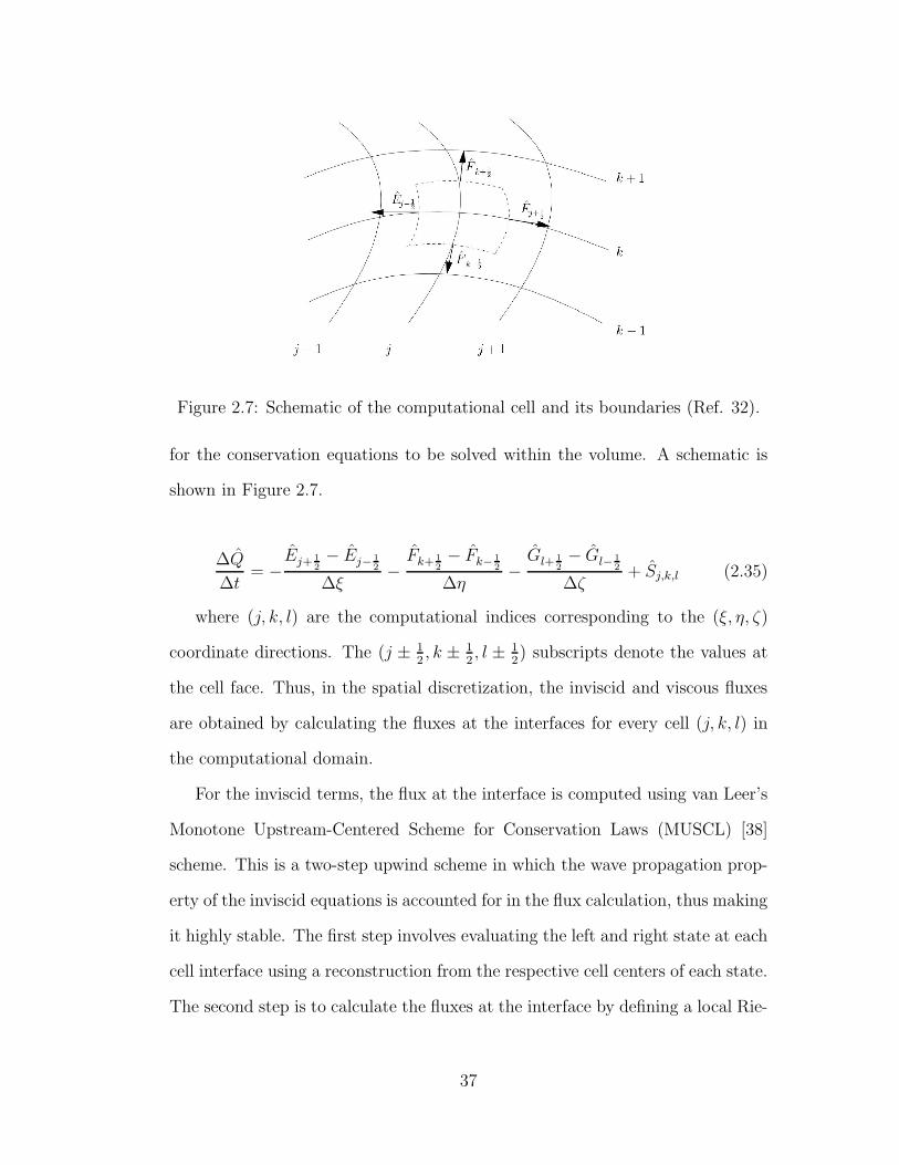
Figure 2.7: Schematic of the computational cell and its boundaries (Ref. 32).

for the conservation equations to be solved within the volume. A schematic is

shown in Figure 2.7.

∆Q

∆t= −

Ej+ 1

2

− Ej− 1

2

∆ξ−

Fk+ 1

2

− Fk− 1

2

∆η−

Gl+ 1

2

− Gl− 1

2

∆ζ+ Sj,k,l (2.35)

where (j, k, l) are the computational indices corresponding to the (ξ, η, ζ)

coordinate directions. The (j ± 1

2, k ± 1

2, l ± 1

2) subscripts denote the values at

the cell face. Thus, in the spatial discretization, the inviscid and viscous fluxes

are obtained by calculating the fluxes at the interfaces for every cell (j, k, l) in

the computational domain.

For the inviscid terms, the flux at the interface is computed using van Leer’s

Monotone Upstream-Centered Scheme for Conservation Laws (MUSCL) [38]

scheme. This is a two-step upwind scheme in which the wave propagation prop-

erty of the inviscid equations is accounted for in the flux calculation, thus making

it highly stable. The first step involves evaluating the left and right state at each

cell interface using a reconstruction from the respective cell centers of each state.

The second step is to calculate the fluxes at the interface by defining a local Rie-

37

mann problem using the left and right states. In TURNS, Roe flux-difference

splitting [39] is used to solve for the flux at the interface:

F(

qL, qR)

=F(

qL)

+ F(

qR)

2−∣

∣

∣A(

qL, qR)

∣

∣

∣

qR − qL

2(2.36)

In the above equation, A denotes the Roe-averaged Jacobian matrix and L and

R superscripts indicate the left and right states, respectively. Typically Roe’s

scheme is modified by Turkel to become the Roe-Turkel scheme [40] in order to

better approximate low Mach number flow.

In low-Reynolds flows with thick boundary layers and large amounts of sepa-

ration, the viscous terms in the spatial discretization cannot be neglected. Thus,

an example viscous term of the form:

∂

∂ξ

(

α∂β

∂η

)

(2.37)

is discretized in TURNS using a second-order central differencing scheme:

1

∆ξ

[(

αj+ 1

2,k

βj+ 1

2,k+1 − βj+ 1

2,k

∆η

)

−(

αj− 1

2,k

βj− 1

2,k − βj− 1

2,k−1

∆η

)]

(2.38)

where

α, βj± 1

2,k =

α, βj,k ± α, βj±1,k

2(2.39)

2.4.5 Preconditioning

Since the cyclocopter operates in low-Mach and low-Reynolds Number flight

regimes, it is necessary to employ a low-Mach preconditioner to help maintain ac-

curacy and converge the compressible Navier-Stokes flow solver. The discretized

38

form of the compressible Navier-stokes equations does not converge upon the

incompressible solution as Mach number approaches zero. Thus, use of the pre-

conditioner resolves this issue and achieves several specific goals, among which

two are listed below.

• Since there is a large difference between eigenvalues in low Mach flows, the

solution is computationally stiff and therefore requires more time to reach

a steady-state solution. The preconditioner accelerates convergence by

bringing the magnitude of the acoustic eigenvalues closer to the convective

eigenvalues, thereby reducing stiffness.

• A low-Mach preconditioner removes scaling inaccuracies between dissipa-

tion terms. This is most beneficial near the stagnation term and near sur-

face boundary layers, since the preconditioner makes the pressure terms

and convective terms more consistent to each other.

2.4.6 Implicit Time Marching and Dual Time-Stepping

The spatial discretization as described earlier solves for the fluxes at the right-

hand side (RHS) of equation 2.35. Now, the conservative variables, Q, can be

evolved in time. In most CFD solvers, implicit time marching is preferred over

explicit schemes due to the lack of a numerical stability limit. Explicit schemes

only solve the governing equations at a later timestep t + ∆t using information

from the current state of the system. However, they require an impracticably

small ∆t to converge stiff problems while keeping the error bounded, and can

diverge with a larger timestep size. Implicit methods, conversely, solve simul-

taneously at both at the current timestep, t, and the next timestep, t + ∆t.

Hence, implicit schemes do not suffer from the same stability problems, and a

39

larger timestep can be taken to converge the solution faster. When Equation

2.35 is written in a generic discretized ‘delta form’ using an implicit algorithm,

the following expression is obtained:

LHS∆Qn = −∆tRHS (2.40)

Where the right-hand side (RHS) represents the fluxes that comprise the

“physics” of the problem, and the left-hand side represents the implicit scheme

which comprise the “numerics” and determine the rate of convergence. n denotes

the current timestep. The implicit algorithm produces a large sparse banded ma-

trix, which is then solved to obtain a solution for ∆Qn. Typically, approximate

factorization methods are used to solve such sparse systems.

For time-dependent calculations, such as the unsteady moving mesh problems

associated with rotorcraft, dual timestepping [41] may be used to aid in conver-

gence. With dual time-stepping, a series of “pseudo-timesteps” are introduced

per physical time step, such that the unsteady problem becomes a pseudo-steady

problem. Thus, certain advantages of a steady-state problem are attained. How-

ever, care must be taken to ensure that the dual timestepping scheme undergoes

enough sub-iterations such that an accurate transient solution is achieved. Typ-

ically, a drop in the unsteady residual of two orders of magnitude is sufficient to

ensure that each physical timestep is well-converged.

2.4.7 Boundary Conditions

Figure 2.8 shows a schematic of the different types of numerical boundary condi-

tions encountered in the overset blade/background mesh system. The following

list describes the various boundary conditions shown in the schematic and their

40

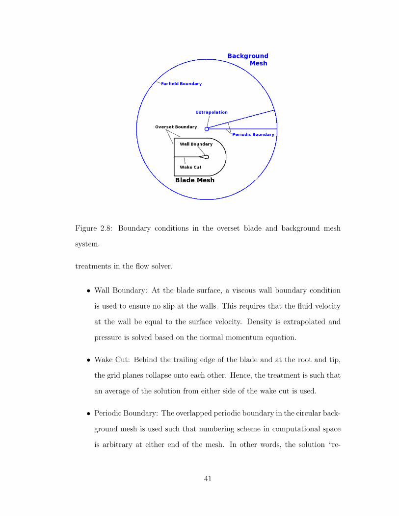
Figure 2.8: Boundary conditions in the overset blade and background mesh

system.

treatments in the flow solver.

• Wall Boundary: At the blade surface, a viscous wall boundary condition

is used to ensure no slip at the walls. This requires that the fluid velocity

at the wall be equal to the surface velocity. Density is extrapolated and

pressure is solved based on the normal momentum equation.

• Wake Cut: Behind the trailing edge of the blade and at the root and tip,

the grid planes collapse onto each other. Hence, the treatment is such that

an average of the solution from either side of the wake cut is used.

• Periodic Boundary: The overlapped periodic boundary in the circular back-

ground mesh is used such that numbering scheme in computational space

is arbitrary at either end of the mesh. In other words, the solution “re-

41

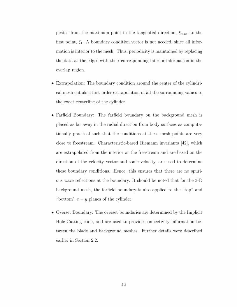
peats” from the maximum point in the tangential direction, ξmax, to the

first point, ξ1. A boundary condition vector is not needed, since all infor-

mation is interior to the mesh. Thus, periodicity is maintained by replacing

the data at the edges with their corresponding interior information in the

overlap region.

• Extrapolation: The boundary condition around the center of the cylindri-

cal mesh entails a first-order extrapolation of all the surrounding values to

the exact centerline of the cylinder.

• Farfield Boundary: The farfield boundary on the background mesh is

placed as far away in the radial direction from body surfaces as computa-

tionally practical such that the conditions at these mesh points are very

close to freestream. Characteristic-based Riemann invariants [42], which

are extrapolated from the interior or the freestream and are based on the

direction of the velocity vector and sonic velocity, are used to determine

these boundary conditions. Hence, this ensures that there are no spuri-

ous wave reflections at the boundary. It should be noted that for the 3-D

background mesh, the farfield boundary is also applied to the “top” and

“bottom” x − y planes of the cylinder.

• Overset Boundary: The overset boundaries are determined by the Implicit

Hole-Cutting code, and are used to provide connectivity information be-

tween the blade and background meshes. Further details were described

earlier in Section 2.2.

42

2.4.8 Specific Methods used in OVERTURNS

The OVERTURNS structured overset solver uses the diagonal form of the im-

plicit approximate factorization method developed by Pulliam and Chaussee [43]

with a preconditioned dual-time scheme to solve the compressible RANS equa-

tions. Computations were performed in the inertial frame in a time-accurate

manner. A third-order MUSCL scheme with Roe flux difference splitting and

Koren’s limiter was used to compute the inviscid terms, and second-order cen-

tral differencing was used for the viscous terms. These were discussed previously

in Section 2.4.4. The low-Mach preconditioner [40] based on Turkel’s method

accelerated the convergence and ensured accuracy of the solution. The Spalart-

Allmaras [37] turbulence model for RANS closure was utilized in 3-D calcula-

tions. However, due to convergence problems with the Spalart-Allmaras model in

the 2-D CFD simulation, the Baldwin-Lomax [36] model was employed. Specific

details beyond the scope of this work with respect to the spatial and temporal

discretization as well as other numerical schemes used in OVERTURNS can be

found in [24].

2.5 Summary

In this chapter, the major steps that must be taken for all CFD approaches were

discussed. These steps are enumerated and summarized in detail below:

1. A mesh must first be generated that resolves the geometry and provides

sufficient resolution to capture the flow features. For the cyclocopter, the

body-fitted curvilinear C-O blade mesh was generated with hyperbolic grid

generation, and the cylindrical background mesh was generated with al-

43

gebraic methods, specifically Vinokur’s stretching procedure in the radial

and spanwise directions away from the rotor cage.

2. To determine the connectivity information for overset meshes, “donor”

and “receiver” cells must be found which are relatively equivalent in size to

interpolate information between meshes without loss of too much accuracy.

For this work, the Implicit Hole-Cutting procedure of Lakshminarayan was

used.

3. A high-fidelity model of the cyclocopter experiment required the unsteady

motion of the blade and its deformations to be prescribed. To this end, a

global rotational motion was imposed on the blade mesh and the numerical

approximation to the four-bar mechanism used by Parsons and Benedict

was used to define the pitching motion. Structural deformations were pre-

scribed onto the blade mesh in TURNS using the methodology developed

by Sitaraman.

4. The flow solver uses the compressible Reynolds-Averaged Navier-Stokes

(RANS) equations, which comprise mass, momentum, and energy con-

servation, to solve for the flowfield. The Baldwin-Lomax and Spalart-

Allmaras models were both used in this work to provide closure to the

RANS equations. These equations are then are converted from physical

space to computational space via a curvilinear coordinate transformation

such that the flux contributions can be defined with respect to adjacent

cell faces. The finite-volume approach is used in TURNS for discretization,

and cell interface fluxes are evaluated to allow for the conservation equa-

tions to be solved within the volume. Preconditioning is employed to help

44

convergence of the compressible RANS equations at low Mach numbers.

An implicit time discretization is used with dual time-stepping to maintain

accuracy.

5. Boundary conditions must be prescribed onto the grid before starting the

flow solver. Types of boundary conditions used specifically in this work

are wall boundaries, wake cuts, periodic boundaries, extrapolations, farfield

boundaries, and overset boundaries.

Utilizing the above numerical methods together, a flow solution can be ob-

tained for a desired computational mesh. However, before solving for a complex

case such as the cyclocopter, the flow solver must first be validated on simpler

geometries.

45

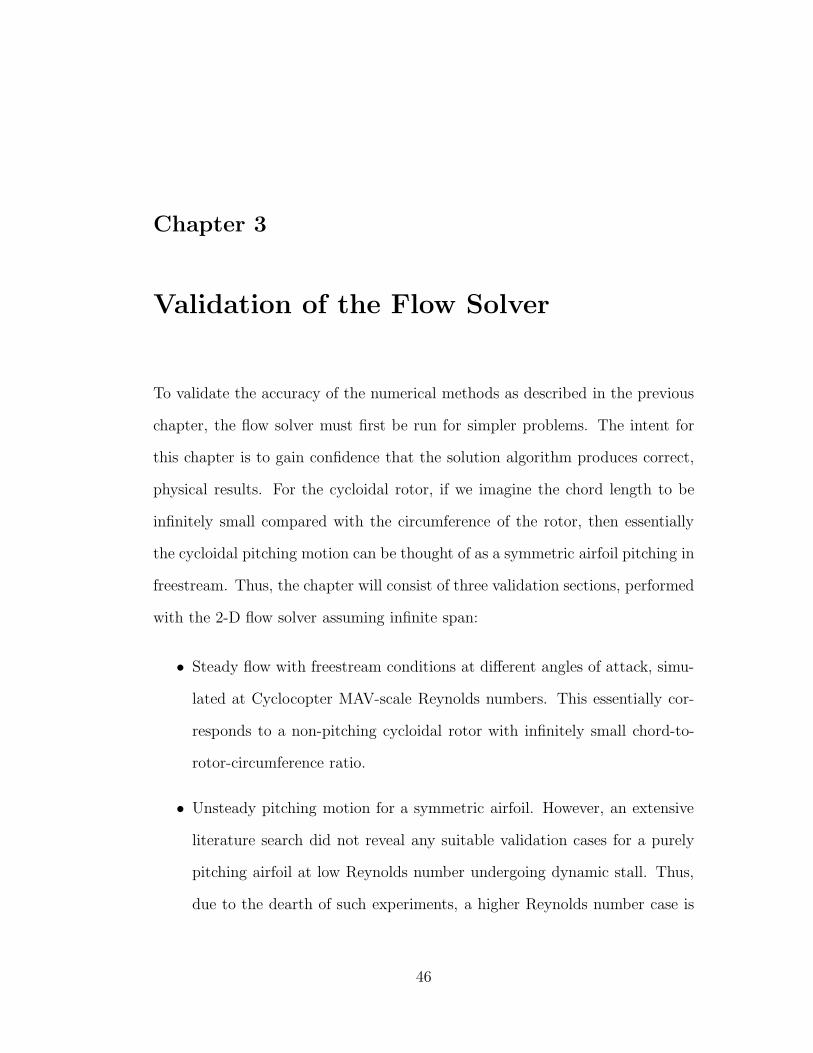
Chapter 3

Validation of the Flow Solver

To validate the accuracy of the numerical methods as described in the previous

chapter, the flow solver must first be run for simpler problems. The intent for

this chapter is to gain confidence that the solution algorithm produces correct,

physical results. For the cycloidal rotor, if we imagine the chord length to be

infinitely small compared with the circumference of the rotor, then essentially

the cycloidal pitching motion can be thought of as a symmetric airfoil pitching in

freestream. Thus, the chapter will consist of three validation sections, performed

with the 2-D flow solver assuming infinite span:

• Steady flow with freestream conditions at different angles of attack, simu-

lated at Cyclocopter MAV-scale Reynolds numbers. This essentially cor-

responds to a non-pitching cycloidal rotor with infinitely small chord-to-

rotor-circumference ratio.

• Unsteady pitching motion for a symmetric airfoil. However, an extensive

literature search did not reveal any suitable validation cases for a purely

pitching airfoil at low Reynolds number undergoing dynamic stall. Thus,

due to the dearth of such experiments, a higher Reynolds number case is

46

used for validation.

• Unsteady rotational motion of a symmetric airfoil at low Reynolds num-

bers. This examines the capabilities of the solver to produce accurate

results at high angles of attack and explores the highly separated flowfield

characteristic of this type of unsteady blade motion. As there were no

MAV-scale cycloidal rotor cases in experiment for comparison, a VAWT

result is used.

CFD simulations were also performed for an unsteady pitching NACA 0010

airfoil at Re = 30, 000, M∞ = 0.047 corresponding to the flight regime of Bene-

dict et al.’s experiments [14], there was no experimental validation for this work.

The predictions of unsteady time histories for Cl, Cd, and Cm from this simula-

tion are shown in Appendix B. Without verification from experiment, though,

the results presented in that section should only be treated as computational

predictions and not definitive, accurate results.

3.1 Steady Airfoil Validation

The low-Reynolds number airfoil experiments of Lutz et al. [44] were used to

validate the steady 2-D solver. Lutz took lift and drag measurements as a

function of angle of attack for a symmetric NACA 0009 airfoil at Re = 50, 000

and M∞ ≈ 0.02.

A 2-D TURNS steady simulation was undertaken with low-Mach precon-

ditioning and the Baldwin-Lomax turbulence model for determination of eddy

viscosity. The grid was a 209 × 154 C airfoil mesh with outer boundaries at 15

chords away from the blade surface, as shown in Figure 3.1. The clustering at

47

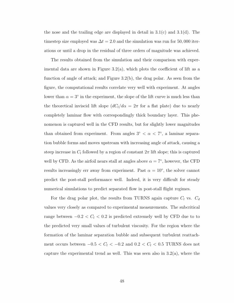
the nose and the trailing edge are displayed in detail in 3.1(c) and 3.1(d). The

timestep size employed was ∆t = 2.0 and the simulation was run for 50, 000 iter-

ations or until a drop in the residual of three orders of magnitude was achieved.

The results obtained from the simulation and their comparison with exper-

imental data are shown in Figure 3.2(a), which plots the coefficient of lift as a

function of angle of attack; and Figure 3.2(b), the drag polar. As seen from the

figure, the computational results correlate very well with experiment. At angles

lower than α = 3◦ in the experiment, the slope of the lift curve is much less than

the theoretical inviscid lift slope (dCl/dα = 2π for a flat plate) due to nearly

completely laminar flow with correspondingly thick boundary layer. This phe-

nomenon is captured well in the CFD results, but for slightly lower magnitudes

than obtained from experiment. From angles 3◦ < α < 7◦, a laminar separa-

tion bubble forms and moves upstream with increasing angle of attack, causing a

steep increase in Cl followed by a region of constant 2π lift slope; this is captured

well by CFD. As the airfoil nears stall at angles above α = 7◦, however, the CFD

results increasingly err away from experiment. Past α = 10◦, the solver cannot

predict the post-stall performance well. Indeed, it is very difficult for steady

numerical simulations to predict separated flow in post-stall flight regimes.

For the drag polar plot, the results from TURNS again capture Cl vs. Cd

values very closely as compared to experimental measurements. The subcritical

range between −0.2 < Cl < 0.2 is predicted extremely well by CFD due to to

the predicted very small values of turbulent viscosity. For the region where the

formation of the laminar separation bubble and subsequent turbulent reattach-

ment occurs between −0.5 < Cl < −0.2 and 0.2 < Cl < 0.5 TURNS does not

capture the experimental trend as well. This was seen also in 3.2(a), where the

48

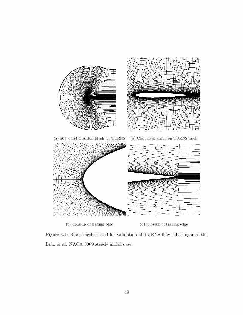
(a) 209 × 154 C Airfoil Mesh for TURNS (b) Closeup of airfoil on TURNS mesh

(c) Closeup of leading edge (d) Closeup of trailing edge

Figure 3.1: Blade meshes used for validation of TURNS flow solver against the

Lutz et al. NACA 0009 steady airfoil case.

49

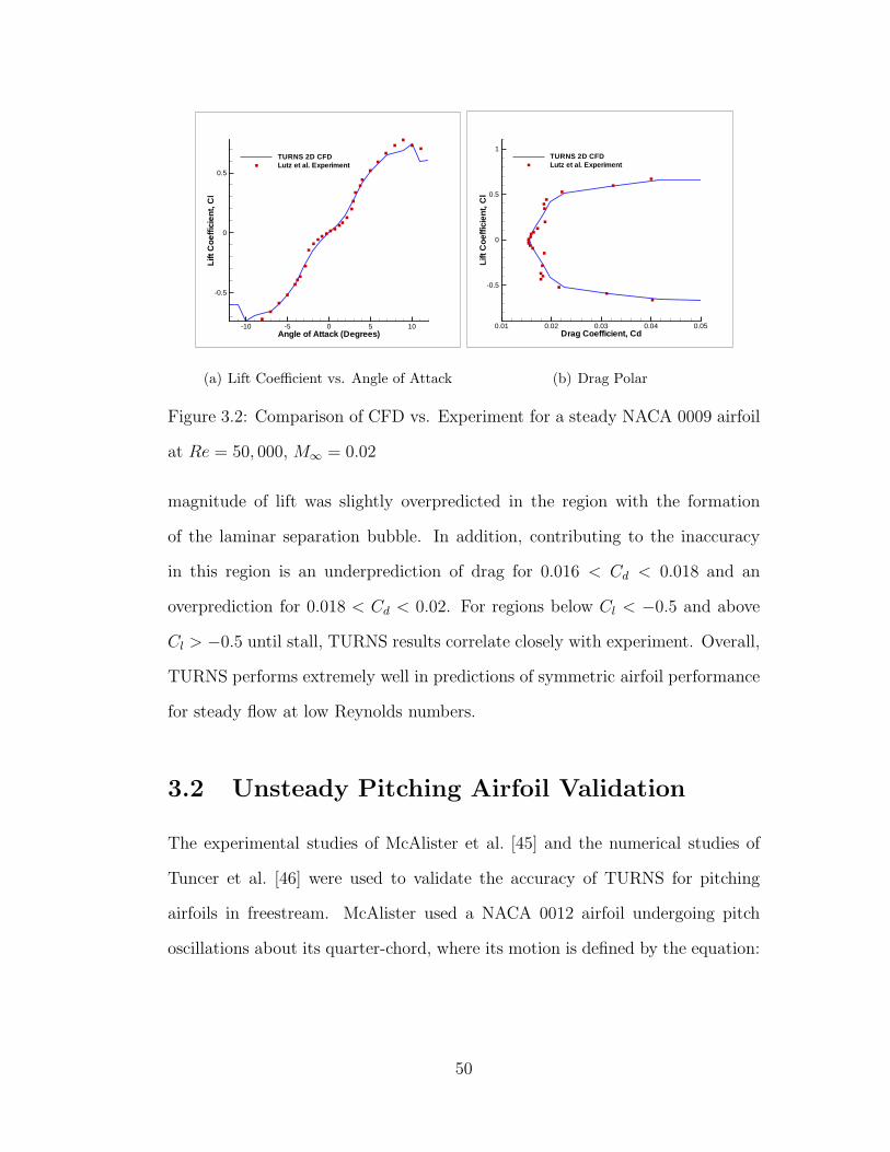
Angle of Attack (Degrees)

Lift

Coe

ffici

ent,

Cl

-10 -5 0 5 10

-0.5

0

0.5

TURNS 2D CFDLutz et al. Experiment

(a) Lift Coefficient vs. Angle of Attack

Drag Coefficient, Cd

Lift

Coe

ffici

ent,

Cl

0.01 0.02 0.03 0.04 0.05

-0.5

0

0.5

1TURNS 2D CFDLutz et al. Experiment

(b) Drag Polar

Figure 3.2: Comparison of CFD vs. Experiment for a steady NACA 0009 airfoil

at Re = 50, 000, M∞ = 0.02

magnitude of lift was slightly overpredicted in the region with the formation

of the laminar separation bubble. In addition, contributing to the inaccuracy

in this region is an underprediction of drag for 0.016 < Cd < 0.018 and an

overprediction for 0.018 < Cd < 0.02. For regions below Cl < −0.5 and above

Cl > −0.5 until stall, TURNS results correlate closely with experiment. Overall,

TURNS performs extremely well in predictions of symmetric airfoil performance

for steady flow at low Reynolds numbers.

3.2 Unsteady Pitching Airfoil Validation

The experimental studies of McAlister et al. [45] and the numerical studies of

Tuncer et al. [46] were used to validate the accuracy of TURNS for pitching

airfoils in freestream. McAlister used a NACA 0012 airfoil undergoing pitch

oscillations about its quarter-chord, where its motion is defined by the equation:

50

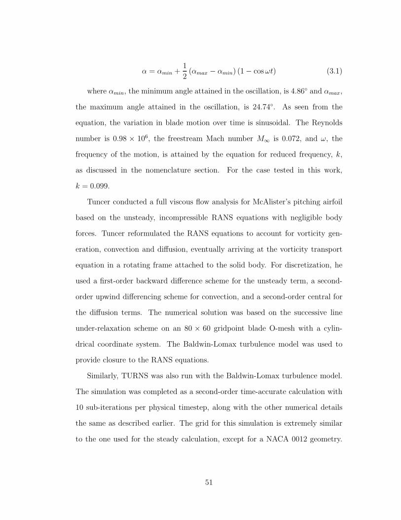
α = αmin +1

2(αmax − αmin) (1 − cos ωt) (3.1)

where αmin, the minimum angle attained in the oscillation, is 4.86◦ and αmax,

the maximum angle attained in the oscillation, is 24.74◦. As seen from the

equation, the variation in blade motion over time is sinusoidal. The Reynolds

number is 0.98 × 106, the freestream Mach number M∞ is 0.072, and ω, the

frequency of the motion, is attained by the equation for reduced frequency, k,

as discussed in the nomenclature section. For the case tested in this work,

k = 0.099.

Tuncer conducted a full viscous flow analysis for McAlister’s pitching airfoil

based on the unsteady, incompressible RANS equations with negligible body

forces. Tuncer reformulated the RANS equations to account for vorticity gen-

eration, convection and diffusion, eventually arriving at the vorticity transport

equation in a rotating frame attached to the solid body. For discretization, he

used a first-order backward difference scheme for the unsteady term, a second-

order upwind differencing scheme for convection, and a second-order central for

the diffusion terms. The numerical solution was based on the successive line

under-relaxation scheme on an 80 × 60 gridpoint blade O-mesh with a cylin-

drical coordinate system. The Baldwin-Lomax turbulence model was used to

provide closure to the RANS equations.

Similarly, TURNS was also run with the Baldwin-Lomax turbulence model.

The simulation was completed as a second-order time-accurate calculation with

10 sub-iterations per physical timestep, along with the other numerical details

the same as described earlier. The grid for this simulation is extremely similar

to the one used for the steady calculation, except for a NACA 0012 geometry.

51

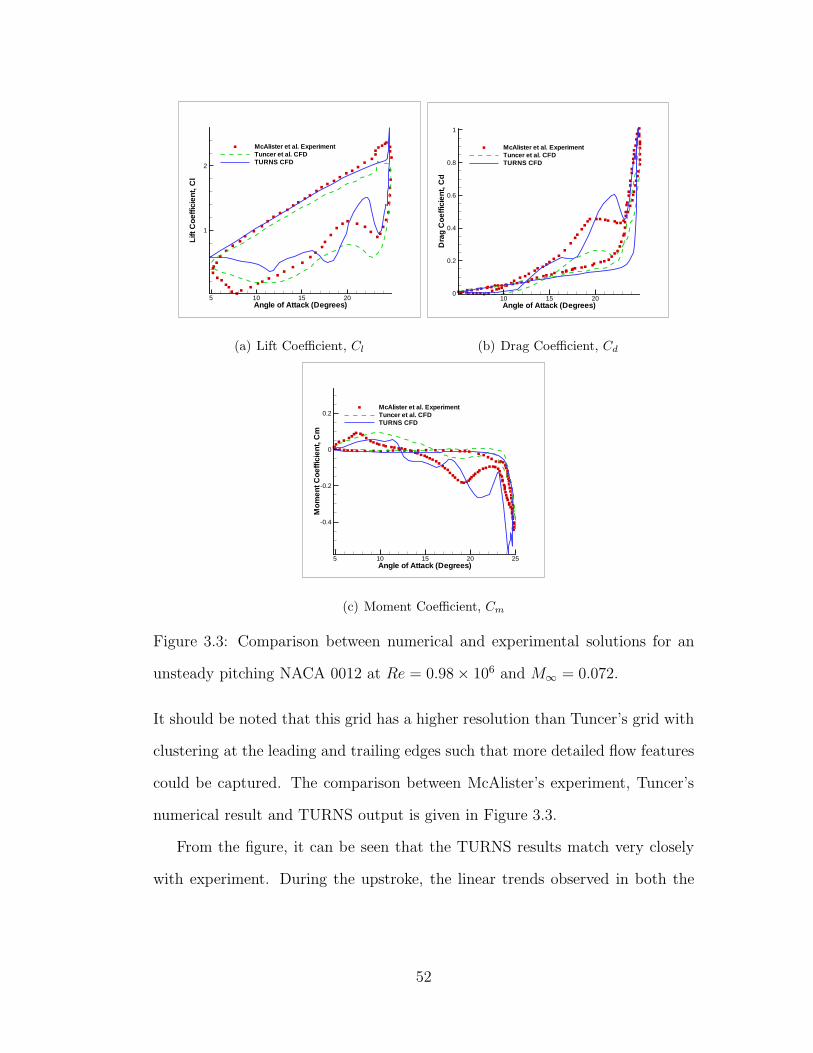
Angle of Attack (Degrees)

Lift

Coe

ffici

ent,

Cl

5 10 15 20

1

2

McAlister et al. ExperimentTuncer et al. CFDTURNS CFD

(a) Lift Coefficient, Cl

Angle of Attack (Degrees)

Dra

gC

oeffi

cien

t,C

d

10 15 200

0.2

0.4

0.6

0.8

1

McAlister et al. ExperimentTuncer et al. CFDTURNS CFD

(b) Drag Coefficient, Cd

Angle of Attack (Degrees)

Mom

entC

oeffi

cien

t,C

m

5 10 15 20 25

-0.4

-0.2

0

0.2McAlister et al. ExperimentTuncer et al. CFDTURNS CFD

(c) Moment Coefficient, Cm

Figure 3.3: Comparison between numerical and experimental solutions for an

unsteady pitching NACA 0012 at Re = 0.98 × 106 and M∞ = 0.072.

It should be noted that this grid has a higher resolution than Tuncer’s grid with

clustering at the leading and trailing edges such that more detailed flow features

could be captured. The comparison between McAlister’s experiment, Tuncer’s

numerical result and TURNS output is given in Figure 3.3.

From the figure, it can be seen that the TURNS results match very closely

with experiment. During the upstroke, the linear trends observed in both the

52

lift and moment coefficients are better predicted by TURNS (with respect to

experimental data) than Tuncer’s simulation. As the leading edge vortex forms

near α = 25◦, TURNS captures but overpredicts the peak in lift and moment; it

predicts the peak in drag well, but does not capture the upper hysteresis loop.

As the leading edge vortex travels down the chord of the airfoil, it “bursts” at the

trailing edge and sheds clockwise vorticity; this drop is also caught by TURNS.

However, the second local maximum in lift, drag, and negative moment, obtained

on the downstroke at around α = 22◦, is overpredicted by TURNS, whereas it

was previously underpredicted by Tuncer’s results. This local maximum is due

to the suction generated by the trailing edge vortex, and Tuncer offers a reason

as to why this is not well predicted in the numerical simulation: the Baldwin-

Lomax turbulence model does not perform well in the wake region.

Past the shedding of the trailing edge vortex, the lift curve steadily decreases

in experiment due to the reattachment of the trailing edge and the formation

of secondary vortex structures. The flow reattaches on the upper surface past

α = 7◦, and the lift reaches a global minimum before increasing. Again in both

numerical models, the lift curve is not predicted well here, although the drag and

moment curves are slightly improved. Due to the fully turbulent flow assump-

tion, the flow solvers may be forcing the reattachment of the boundary layers

earlier than experiment, thus leading to an overpredicted global maximum. After

the suction on the leading-edge is established, then both flow solvers gravitate

towards the steady-state value of lift, drag, and moment. Overall, though, the

correlation between TURNS and experimental results are fair.

53

3.3 Validation of 2-D Unsteady Flow Separa-

tion from Airfoil Rotation

The experimental results for dynamic stall on a VAWT were used to validate

TURNS’ predictive capability in a highly separated flowfield. Such a flow en-

vironment is characteristic of airfoil movement around a rotor cage with a high

chord-to-rotor-circumference ratio. Ferreira et al. [8] at the Delft University of

Technology conducted Particle Image Velocimetry (PIV) measurements to visu-

alize flow within an H-Darrieus type straight-bladed vertical axis wind turbine

with no blade pitch, originally developed by Coene [47]. The experimental setup

consisted of a single NACA 0015 airfoil with a chord of 0.05 m, a rotor diameter

of 0.4 m, a rod with a diameter of 0.05 m at the rotational axis, and an aspect

ratio of 20 to produce an almost 2-D case. Flow measurements were taken for

two different mean Reynolds numbers, 52000 and 70000 and three tip speed ra-

tios, λ = 2,3,4, corresponding to each. Furthermore, Ferreira conducted a CFD

simulation [48] using Fluent (a commercial CFD package) for a 7.5 m/s, λ = 2,

and 52000 mean Reynolds number case using different turbulence models and

varying spatial and temporal resolution to validate against PIV data.

A blade shape-conforming mesh of 209 x 94 points on a circular background

mesh of 321 x 251 points with a five-point overlapped boundary condition was

used in OVERTURNS for verification of this case. A schematic of the com-

putational domain as well as the overset grid system is shown in Figure 3.4(a)

and 3.4(b), respectively. The wind tunnel walls are not replicated in the OVER-

TURNS simulation, as Ferreira et al. stated that the effect of the walls was negli-

54

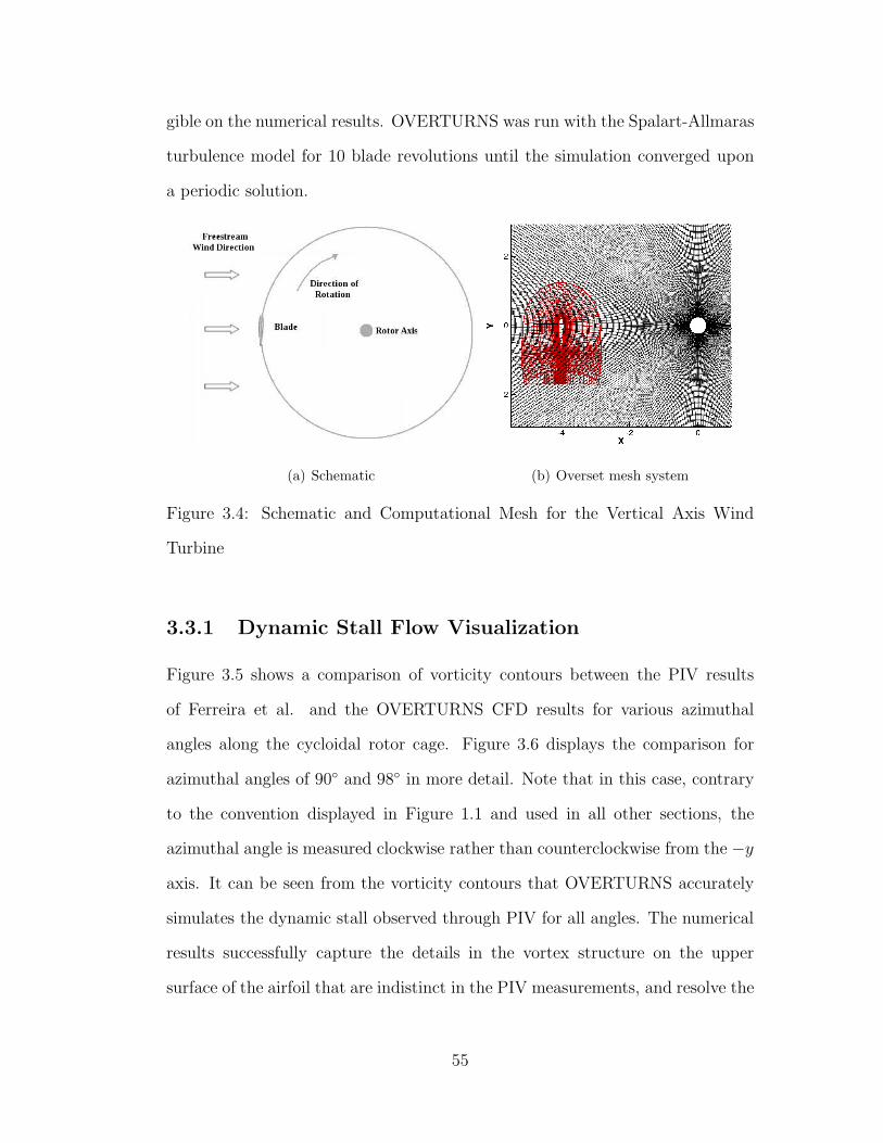
gible on the numerical results. OVERTURNS was run with the Spalart-Allmaras

turbulence model for 10 blade revolutions until the simulation converged upon

a periodic solution.

(a) Schematic (b) Overset mesh system

Figure 3.4: Schematic and Computational Mesh for the Vertical Axis Wind

Turbine

3.3.1 Dynamic Stall Flow Visualization

Figure 3.5 shows a comparison of vorticity contours between the PIV results

of Ferreira et al. and the OVERTURNS CFD results for various azimuthal

angles along the cycloidal rotor cage. Figure 3.6 displays the comparison for

azimuthal angles of 90◦ and 98◦ in more detail. Note that in this case, contrary

to the convention displayed in Figure 1.1 and used in all other sections, the

azimuthal angle is measured clockwise rather than counterclockwise from the −y

axis. It can be seen from the vorticity contours that OVERTURNS accurately

simulates the dynamic stall observed through PIV for all angles. The numerical

results successfully capture the details in the vortex structure on the upper

surface of the airfoil that are indistinct in the PIV measurements, and resolve the

55

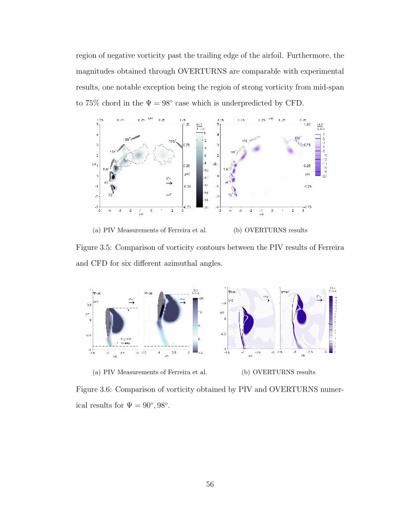
region of negative vorticity past the trailing edge of the airfoil. Furthermore, the

magnitudes obtained through OVERTURNS are comparable with experimental

results, one notable exception being the region of strong vorticity from mid-span

to 75% chord in the Ψ = 98◦ case which is underpredicted by CFD.

(a) PIV Measurements of Ferreira et al. (b) OVERTURNS results

Figure 3.5: Comparison of vorticity contours between the PIV results of Ferreira

and CFD for six different azimuthal angles.

(a) PIV Measurements of Ferreira et al. (b) OVERTURNS results

Figure 3.6: Comparison of vorticity obtained by PIV and OVERTURNS numer-

ical results for Ψ = 90◦, 98◦.

56

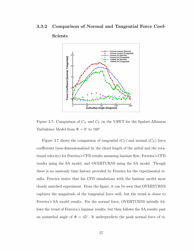
3.3.2 Comparison of Normal and Tangential Force Coef-

ficients

Azimuthal Angle (Degrees)

For

ceC

oeffi

cien

t(N

orm

al,T

ange

ntia

l)

0 45 90 135 180

0

1

2

3

4

Ferreira Laminar (Normal)Ferreira Laminar (Tangential)Ferreira SA (Normal)Ferreira SA (Tangential)TURNS SA (Normal)TURNS SA (Tangential)

Figure 3.7: Comparison of CN and CT on the VAWT for the Spalart-Allmaras

Turbulence Model from Ψ = 0◦ to 180◦

Figure 3.7 shows the comparison of tangential (CT ) and normal (CN) force

coefficients (non-dimensionalized by the chord length of the airfoil and the rota-

tional velocity) for Ferreira’s CFD results assuming laminar flow, Ferreira’s CFD

results using the SA model, and OVERTURNS using the SA model. Though

there is no unsteady time history provided by Ferreira for the experimental re-

sults, Ferreira states that his CFD simulations with the laminar model most

closely matched experiment. From the figure, it can be seen that OVERTURNS

captures the magnitude of the tangential force well, but the trend is closer to

Ferreira’s SA model results. For the normal force, OVERTURNS initially fol-

lows the trend of Ferreira’s laminar results, but then follows the SA results past

an azimuthal angle of Ψ = 45◦. It underpredicts the peak normal force of ei-

57

ther Ferreira’s SA or laminar models at Ψ = 90◦. After 90◦ azimuth, it again

begins following the trend of the laminar model. Despite the underprediction

of magnitude, the TURNS results may better predict unsteady shedding than

Ferreira’s SA results and may be closer to experiment since it mostly follows

the laminar model. To reinforce this, Ferreira stated that his laminar simulation

better captures the development of the large leading edge separated vorticity

and the rolling up of the counter-clockwise vorticity at the trailing edge past the

Ψ = 90◦ location which he observed in experiment; this phenomenon manifests

as a rapid drop in CN for the laminar time history in Figure 3.7. TURNS predicts

this drop as well, despite the fact that using the SA model assumes fully tur-

bulent flow. Ferreira previously stated that his SA simulations had suppressed

the development of the leading edge separation at this azimuthal location and

therefore deviated from experiment. However, since OVERTURNS captures this

even with a fully turbulent assumption, OVERTURNS is seen to correlate better

with Ferreira’s laminar results and therefore predict results closer to experiment.

3.4 Summary

As seen from this section, TURNS predicts reasonably well the performance of

steady airfoils at low Reynolds numbers and unsteady pitching airfoils. It was

shown that:

• While TURNS captures the trends for the steady NACA 0009 airfoil at

Re = 50, 000 extremely well, the region between −5◦ < α < 5◦ where

the laminar separation bubble forms is slightly less well captured as the

magnitude of Cl is slightly overpredicted, and Cd is slightly under-, then

58

overpredicted for this region.

• For the unsteady pitching airfoil results, the linear trends observed during

the upstroke in the lift and moment coefficients correlate very closely with

experiment, and are predicted better than Tuncer’s simulation. TURNS

overpredicts the lift and moment peaks, however, and underpredicts the

drag peak. On the downstroke, it does not captured regions of separated

flow well, and as a result deviates somewhat from experiment. Overall,

however, trends match relatively well between TURNS and McAlister’s

experiments.

• The unsteady airfoil rotation to test TURNS’ predictive capability for

highly separated flow showed that quantitatively, TURNS performed well

in capturing the flowfield seen in Ferreira’s PIV results. Qualitatively,

TURNS predicted CT well, and TURNS more closely followed the laminar

(and therefore experimental) trend in the unsteady CN time history despite

using the SA model with a fully turbulent assumption. This suggests that

this assumption is not altogether inappropriate for the TURNS flow solver

in the low Reynolds, low Mach unsteady flow environment characteristic

of both VAWTs and MAV-scale cycloidal rotors.

The validation of these simple cases allows the creation of a basic framework

upon which more difficult cases can be tested, with the confidence that the

results produced by the numerical solver are physically accurate. In the following

chapter, numerical simulations of the cyclocopter will be described in detail and

the performance results from the solver will be compared with experiment.

59

Chapter 4

Comparison of Cycloidal Rotor CFD

Results with Experiment

With validation of the solver achieved from the previous chapter, the current

chapter describes CFD pertaining specifically to the cyclocopter, including nu-

merical methods employed to emulate the experiment to a high level of accuracy.

Comparisons between CFD predictions and experimental measurements will be

presented in the latter sections.

4.1 Experimental Setup for Validation

For the cycloidal rotor, experimental results of Benedict et al. [14] were used to

validate the predictions of the 2-D and 3-D flow solvers. Benedict et al. tested

both twin- and quad-rotor MAV-scale cyclocopter configurations with two to

five blades per rotor cage. He used a symmetric airfoil with design attributes

listed in Table 4.1. Figure 4.1 shows the experimental setup. The blades were

constrained at the root and tip onto two carbon fiber end plates connected by

a carbon fiber rod in the center. Measurements of vertical and sidewise force

60

(a) 2-bladed cycloidal rotor cage (b) Experimental measurement setup

Figure 4.1: Experimental setup of Benedict et al. (Ref. 16)

were obtained on the cyclocopter using a thrust load cell. A torque cell was used

to measure the torque which, when combined with Hall sensor measurements of

the rotor RPM, allowed for calculation of total power. In turn, the aerodynamic

power was obtained by taking the total measured power and subtracting the

power consumed by spinning the structure without blades.

Parameter Value

Chord Length 0.0274m

Radius 0.0706m

Span 0.1411m

Number of Blades 2 − 5

Rotating Speed 400 − 2000RPM

Maximum Pitch Angle 25◦ − 40◦

Airfoil Section NACA 0010

Table 4.1: Cyclocopter design parameters based on the experimental setup of

Benedict et al.

61

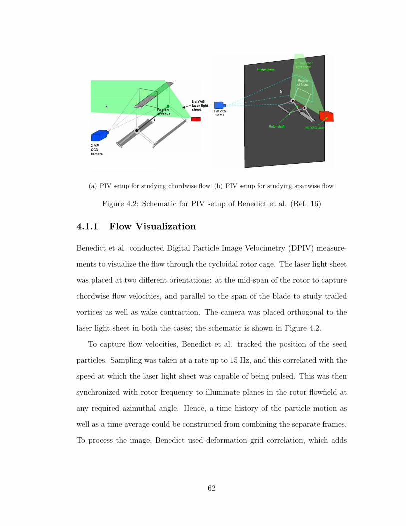
(a) PIV setup for studying chordwise flow (b) PIV setup for studying spanwise flow

Figure 4.2: Schematic for PIV setup of Benedict et al. (Ref. 16)

4.1.1 Flow Visualization

Benedict et al. conducted Digital Particle Image Velocimetry (DPIV) measure-

ments to visualize the flow through the cycloidal rotor cage. The laser light sheet

was placed at two different orientations: at the mid-span of the rotor to capture

chordwise flow velocities, and parallel to the span of the blade to study trailed

vortices as well as wake contraction. The camera was placed orthogonal to the

laser light sheet in both the cases; the schematic is shown in Figure 4.2.

To capture flow velocities, Benedict et al. tracked the position of the seed

particles. Sampling was taken at a rate up to 15 Hz, and this correlated with the

speed at which the laser light sheet was capable of being pulsed. This was then

synchronized with rotor frequency to illuminate planes in the rotor flowfield at

any required azimuthal angle. Hence, a time history of the particle motion as

well as a time average could be constructed from combining the separate frames.

To process the image, Benedict used deformation grid correlation, which adds

62

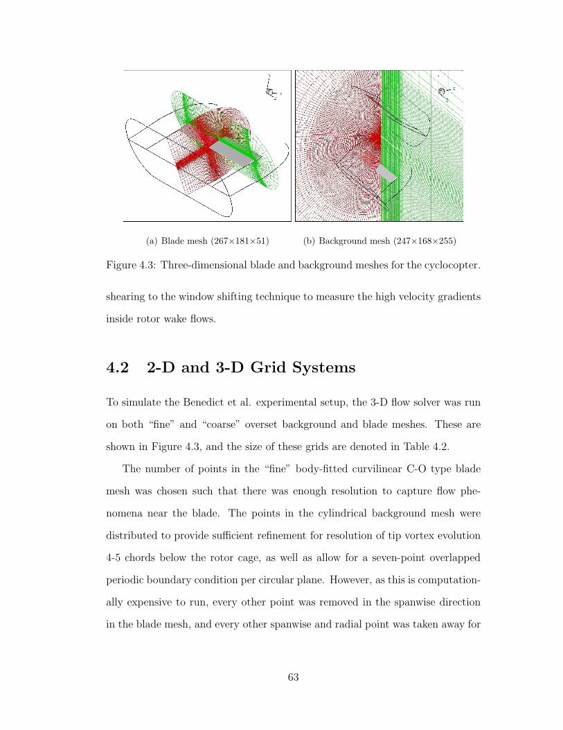
(a) Blade mesh (267×181×51) (b) Background mesh (247×168×255)

Figure 4.3: Three-dimensional blade and background meshes for the cyclocopter.

shearing to the window shifting technique to measure the high velocity gradients

inside rotor wake flows.

4.2 2-D and 3-D Grid Systems

To simulate the Benedict et al. experimental setup, the 3-D flow solver was run

on both “fine” and “coarse” overset background and blade meshes. These are

shown in Figure 4.3, and the size of these grids are denoted in Table 4.2.

The number of points in the “fine” body-fitted curvilinear C-O type blade

mesh was chosen such that there was enough resolution to capture flow phe-

nomena near the blade. The points in the cylindrical background mesh were

distributed to provide sufficient refinement for resolution of tip vortex evolution

4-5 chords below the rotor cage, as well as allow for a seven-point overlapped

periodic boundary condition per circular plane. However, as this is computation-

ally expensive to run, every other point was removed in the spanwise direction

in the blade mesh, and every other spanwise and radial point was taken away for

63

the background mesh to comprise a “coarse” overset mesh. This “coarse” mesh

was used to predict rotor performance and compare to the thrust and power

values obtained from experiment. However, from Figure 4.4, which compares

forces obtained from one cyclocopter blade starting at Ψ = 0◦ with 40◦ pitch

amplitude and 1400 RPM, it can be seen that the time histories of the coarse

and fine mesh are nearly identical, and this indicates grid convergence.

The 2-D grids were taken at the mid-span section of the fine mesh. 2-D

runs were used to gain quick insight into the physics of the flowfield without

the computational cost of the 3-D runs. In addition, when compared to the 3-D

runs, the 2-D runs provide an anchor to explore the effect of three-dimensionality

on the flowfield, as 2-D assumes infinite span. As will be discussed later in

Chapter 4.4, while the 2-D results provide comparable results to 3-D with regard

to performance predictions, the qualitative comparison of the flowfield shows

significant difference in flow phenomena captured.

Though the cylindrical background mesh was used for all cyclocopter CFD

runs, another background grid was generated with the purpose of capturing more

Coarse Mesh Fine Mesh

Blade

Tangential 267 267

Normal 51 51

Spanwise 181 91

Background

Tangential 247 247

Radial 168 84

Spanwise 255 128

Table 4.2: Number of grid points in both fine and coarse background and blade

meshes.

64

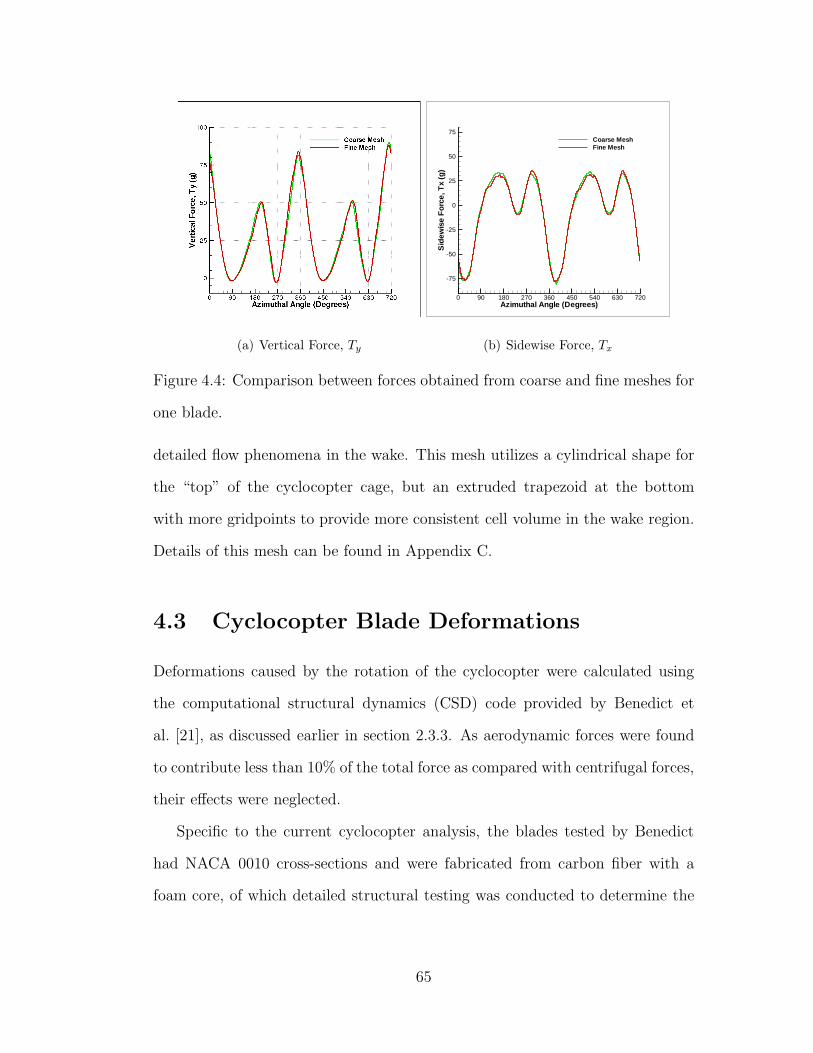
(a) Vertical Force, Ty

Azimuthal Angle (Degrees)

Sid

ewis

eF

orce

,Tx

(g)

0 90 180 270 360 450 540 630 720

-75

-50

-25

0

25

50

75Coarse MeshFine Mesh

(b) Sidewise Force, Tx

Figure 4.4: Comparison between forces obtained from coarse and fine meshes for

one blade.

detailed flow phenomena in the wake. This mesh utilizes a cylindrical shape for

the “top” of the cyclocopter cage, but an extruded trapezoid at the bottom

with more gridpoints to provide more consistent cell volume in the wake region.

Details of this mesh can be found in Appendix C.

4.3 Cyclocopter Blade Deformations

Deformations caused by the rotation of the cyclocopter were calculated using

the computational structural dynamics (CSD) code provided by Benedict et

al. [21], as discussed earlier in section 2.3.3. As aerodynamic forces were found

to contribute less than 10% of the total force as compared with centrifugal forces,

their effects were neglected.

Specific to the current cyclocopter analysis, the blades tested by Benedict

had NACA 0010 cross-sections and were fabricated from carbon fiber with a

foam core, of which detailed structural testing was conducted to determine the

65

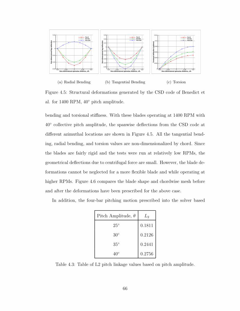
Non-dimensional spanwise distance, z/b

Non

-dim

ensi

onal

flap

defle

ctio

n

-0.5 -0.25 0 0.25 0.5-0.03

-0.02

-0.01

0

0.01

0.02

Psi=0Psi=60Psi=120

(a) Radial Bending

Non-dimensional spanwise distance, z/b

Non

-dim

ensi

onal

lag

defle

ctio

n

-0.5 -0.25 0 0.25 0.5

-0.05

-0.04

-0.03

-0.02

-0.01

0

0.01

0.02

0.03

Psi=0Psi=60Psi=120

(b) Tangential Bending

Non-dimensional spanwise distance, z/b

Tor

sion

alde

flect

ion

(rad

ians

)

-0.5 -0.25 0 0.25 0.50

0.002

0.004

0.006

0.008

0.01

0.012

Psi=0Psi=60Psi=120

(c) Torsion

Figure 4.5: Structural deformations generated by the CSD code of Benedict et

al. for 1400 RPM, 40◦ pitch amplitude.

bending and torsional stiffness. With these blades operating at 1400 RPM with

40◦ collective pitch amplitude, the spanwise deflections from the CSD code at

different azimuthal locations are shown in Figure 4.5. All the tangential bend-

ing, radial bending, and torsion values are non-dimensionalized by chord. Since

the blades are fairly rigid and the tests were run at relatively low RPMs, the

geometrical deflections due to centrifugal force are small. However, the blade de-

formations cannot be neglected for a more flexible blade and while operating at

higher RPMs. Figure 4.6 compares the blade shape and chordwise mesh before

and after the deformations have been prescribed for the above case.

In addition, the four-bar pitching motion prescribed into the solver based

Pitch Amplitude, θ L2

25◦ 0.1811

30◦ 0.2126

35◦ 0.2441

40◦ 0.2756

Table 4.3: Table of L2 pitch linkage values based on pitch amplitude.

66

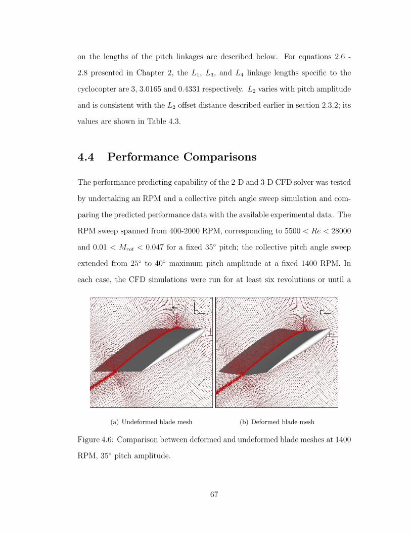
on the lengths of the pitch linkages are described below. For equations 2.6 -

2.8 presented in Chapter 2, the L1, L3, and L4 linkage lengths specific to the

cyclocopter are 3, 3.0165 and 0.4331 respectively. L2 varies with pitch amplitude

and is consistent with the L2 offset distance described earlier in section 2.3.2; its

values are shown in Table 4.3.

4.4 Performance Comparisons

The performance predicting capability of the 2-D and 3-D CFD solver was tested

by undertaking an RPM and a collective pitch angle sweep simulation and com-

paring the predicted performance data with the available experimental data. The

RPM sweep spanned from 400-2000 RPM, corresponding to 5500 < Re < 28000

and 0.01 < Mrot < 0.047 for a fixed 35◦ pitch; the collective pitch angle sweep

extended from 25◦ to 40◦ maximum pitch amplitude at a fixed 1400 RPM. In

each case, the CFD simulations were run for at least six revolutions or until a

(a) Undeformed blade mesh (b) Deformed blade mesh

Figure 4.6: Comparison between deformed and undeformed blade meshes at 1400

RPM, 35◦ pitch amplitude.

67

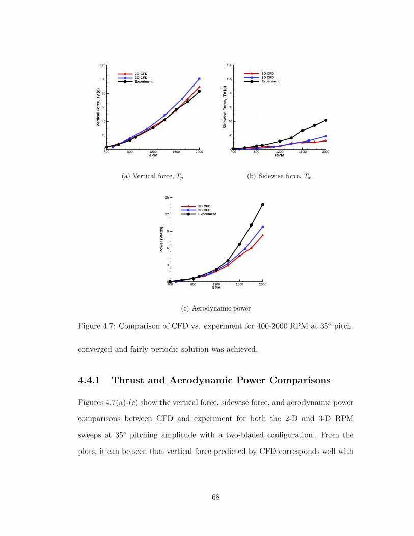
RPM

Ver

tical

For

ce,T

y(g

)

400 800 1200 1600 20000

20

40

60

80

100

120

2D CFD3D CFDExperiment

(a) Vertical force, Ty

RPM

Sid

ewis

eF

orce

,-T

x(g

)

400 800 1200 1600 20000

20

40

60

80

100

120

2D CFD3D CFDExperiment

(b) Sidewise force, Tx

RPM

Pow

er(W

atts

)

400 800 1200 1600 20000

3

6

9

12

15

2D CFD3D CFDExperiment

(c) Aerodynamic power

Figure 4.7: Comparison of CFD vs. experiment for 400-2000 RPM at 35◦ pitch.

converged and fairly periodic solution was achieved.

4.4.1 Thrust and Aerodynamic Power Comparisons

Figures 4.7(a)-(c) show the vertical force, sidewise force, and aerodynamic power

comparisons between CFD and experiment for both the 2-D and 3-D RPM

sweeps at 35◦ pitching amplitude with a two-bladed configuration. From the

plots, it can be seen that vertical force predicted by CFD corresponds well with

68

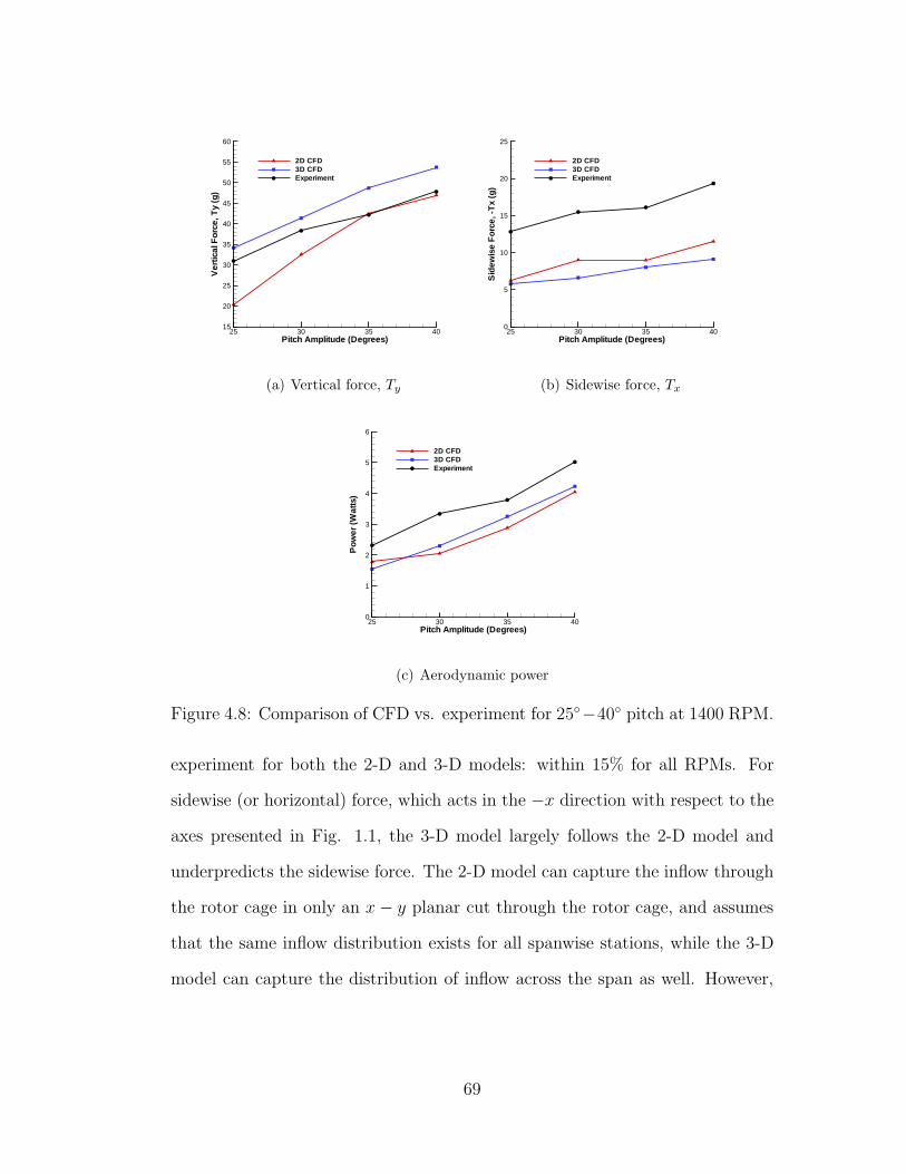
Pitch Amplitude (Degrees)

Ver

tical

For

ce,T

y(g

)

25 30 35 4015

20

25

30

35

40

45

50

55

60

2D CFD3D CFDExperiment

(a) Vertical force, Ty

Pitch Amplitude (Degrees)

Sid

ewis

eF

orce

,-T

x(g

)

25 30 35 400

5

10

15

20

25

2D CFD3D CFDExperiment

(b) Sidewise force, Tx

Pitch Amplitude (Degrees)

Pow

er(W

atts

)

25 30 35 400

1

2

3

4

5

6

2D CFD3D CFDExperiment

(c) Aerodynamic power

Figure 4.8: Comparison of CFD vs. experiment for 25◦−40◦ pitch at 1400 RPM.

experiment for both the 2-D and 3-D models: within 15% for all RPMs. For

sidewise (or horizontal) force, which acts in the −x direction with respect to the

axes presented in Fig. 1.1, the 3-D model largely follows the 2-D model and

underpredicts the sidewise force. The 2-D model can capture the inflow through

the rotor cage in only an x − y planar cut through the rotor cage, and assumes

that the same inflow distribution exists for all spanwise stations, while the 3-D

model can capture the distribution of inflow across the span as well. However,

69

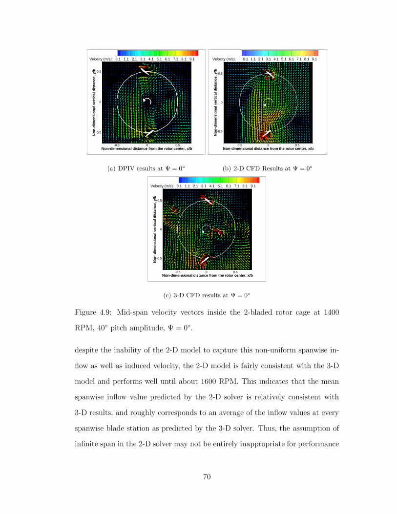
Non-dimensional distance from the rotor center, x/b

Non

-dim

ensi

onal

verti

cald

ista

nce,

y/b

-0.5 0 0.5

-0.5

0

0.5

Velocity (m/s): 0.1 1.1 2.1 3.1 4.1 5.1 6.1 7.1 8.1 9.1

(a) DPIV results at Ψ = 0◦

Non-dimensional distance from the rotor center, x/b

Non

-dim

ensi

onal

verti

cald

ista

nce,

y/b

-0.5 0 0.5

-0.5

0

0.5

Velocity (m/s): 0.1 1.1 2.1 3.1 4.1 5.1 6.1 7.1 8.1 9.1

(b) 2-D CFD Results at Ψ = 0◦

Non-dimensional distance from the rotor center, x/b

Non

-dim

ensi

onal

verti

cald

ista

nce,

y/b

-0.5 0 0.5

-0.5

0

0.5

Velocity (m/s): 0.1 1.1 2.1 3.1 4.1 5.1 6.1 7.1 8.1 9.1

(c) 3-D CFD results at Ψ = 0◦

Figure 4.9: Mid-span velocity vectors inside the 2-bladed rotor cage at 1400

RPM, 40◦ pitch amplitude, Ψ = 0◦.

despite the inability of the 2-D model to capture this non-uniform spanwise in-

flow as well as induced velocity, the 2-D model is fairly consistent with the 3-D

model and performs well until about 1600 RPM. This indicates that the mean

spanwise inflow value predicted by the 2-D solver is relatively consistent with

3-D results, and roughly corresponds to an average of the inflow values at every

spanwise blade station as predicted by the 3-D solver. Thus, the assumption of

infinite span in the 2-D solver may not be entirely inappropriate for performance

70

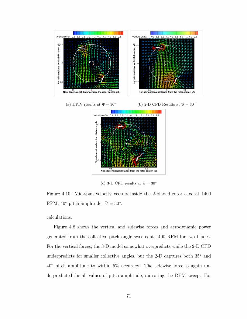
Non-dimensional distance from the rotor center, x/b

Non

-dim

ensi

onal

verti

cald

ista

nce,

y/b

-0.5 0 0.5

-0.5

0

0.5

Velocity (m/s): 0.1 1.1 2.1 3.1 4.1 5.1 6.1 7.1 8.1 9.1

(a) DPIV results at Ψ = 30◦

Non-dimensional distance from the rotor center, x/b

Non

-dim

ensi

onal

verti

cald

ista

nce,

y/b

-0.5 0 0.5

-0.5

0

0.5

Velocity (m/s): 0.1 1.1 2.1 3.1 4.1 5.1 6.1 7.1 8.1 9.1

(b) 2-D CFD Results at Ψ = 30◦

Non-dimensional distance from the rotor center, x/b

Non

-dim

ensi

onal

verti

cald

ista

nce,

y/b

-0.5 0 0.5

-0.5

0

0.5

Velocity (m/s): 0.1 1.1 2.1 3.1 4.1 5.1 6.1 7.1 8.1 9.1

(c) 3-D CFD results at Ψ = 30◦

Figure 4.10: Mid-span velocity vectors inside the 2-bladed rotor cage at 1400

RPM, 40◦ pitch amplitude, Ψ = 30◦.

calculations.

Figure 4.8 shows the vertical and sidewise forces and aerodynamic power

generated from the collective pitch angle sweeps at 1400 RPM for two blades.

For the vertical forces, the 3-D model somewhat overpredicts while the 2-D CFD

underpredicts for smaller collective angles, but the 2-D captures both 35◦ and

40◦ pitch amplitude to within 5% accuracy. The sidewise force is again un-

derpredicted for all values of pitch amplitude, mirroring the RPM sweep. For

71

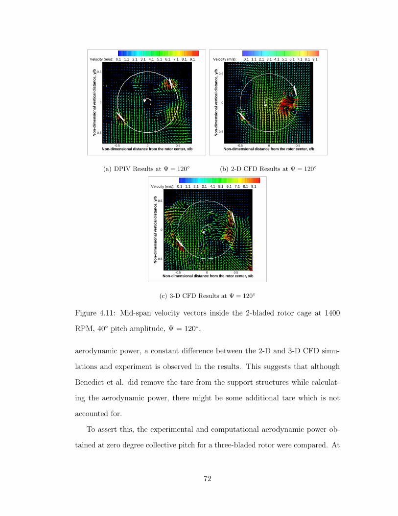
Non-dimensional distance from the rotor center, x/b

Non

-dim

ensi

onal

verti

cald

ista

nce,

y/b

-0.5 0 0.5

-0.5

0

0.5

Velocity (m/s): 0.1 1.1 2.1 3.1 4.1 5.1 6.1 7.1 8.1 9.1

(a) DPIV Results at Ψ = 120◦

Non-dimensional distance from the rotor center, x/b

Non

-dim

ensi

onal

verti

cald

ista

nce,

y/b

-0.5 0 0.5

-0.5

0

0.5

Velocity (m/s): 0.1 1.1 2.1 3.1 4.1 5.1 6.1 7.1 8.1 9.1

(b) 2-D CFD Results at Ψ = 120◦

Non-dimensional distance from the rotor center, x/b

Non

-dim

ensi

onal

verti

cald

ista

nce,

y/b

-0.5 0 0.5

-0.5

0

0.5

Velocity (m/s): 0.1 1.1 2.1 3.1 4.1 5.1 6.1 7.1 8.1 9.1

(c) 3-D CFD Results at Ψ = 120◦

Figure 4.11: Mid-span velocity vectors inside the 2-bladed rotor cage at 1400

RPM, 40◦ pitch amplitude, Ψ = 120◦.

aerodynamic power, a constant difference between the 2-D and 3-D CFD simu-

lations and experiment is observed in the results. This suggests that although

Benedict et al. did remove the tare from the support structures while calculat-

ing the aerodynamic power, there might be some additional tare which is not

accounted for.

To assert this, the experimental and computational aerodynamic power ob-

tained at zero degree collective pitch for a three-bladed rotor were compared. At

72

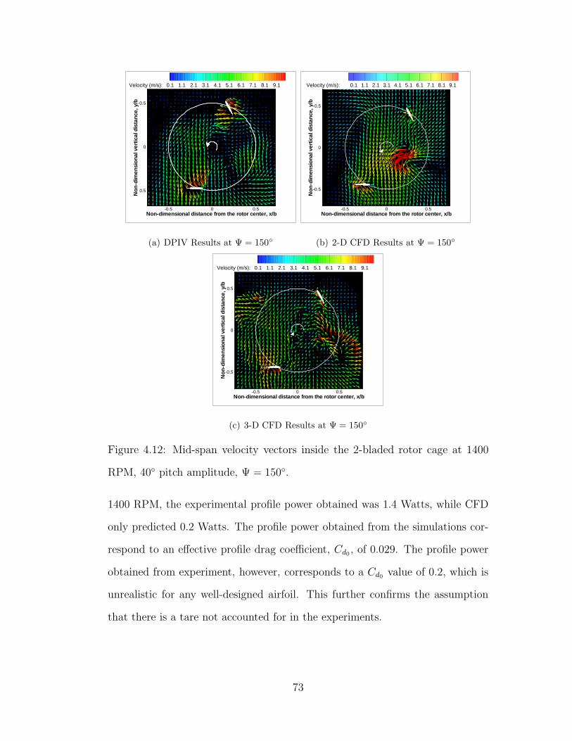
Non-dimensional distance from the rotor center, x/b

Non

-dim

ensi

onal

verti

cald

ista

nce,

y/b

-0.5 0 0.5

-0.5

0

0.5

Velocity (m/s): 0.1 1.1 2.1 3.1 4.1 5.1 6.1 7.1 8.1 9.1

(a) DPIV Results at Ψ = 150◦

Non-dimensional distance from the rotor center, x/b

Non

-dim

ensi

onal

verti

cald

ista

nce,

y/b

-0.5 0 0.5

-0.5

0

0.5

Velocity (m/s): 0.1 1.1 2.1 3.1 4.1 5.1 6.1 7.1 8.1 9.1

(b) 2-D CFD Results at Ψ = 150◦

Non-dimensional distance from the rotor center, x/b

Non

-dim

ensi

onal

verti

cald

ista

nce,

y/b

-0.5 0 0.5

-0.5

0

0.5

Velocity (m/s): 0.1 1.1 2.1 3.1 4.1 5.1 6.1 7.1 8.1 9.1

(c) 3-D CFD Results at Ψ = 150◦

Figure 4.12: Mid-span velocity vectors inside the 2-bladed rotor cage at 1400

RPM, 40◦ pitch amplitude, Ψ = 150◦.

1400 RPM, the experimental profile power obtained was 1.4 Watts, while CFD

only predicted 0.2 Watts. The profile power obtained from the simulations cor-

respond to an effective profile drag coefficient, Cd0, of 0.029. The profile power

obtained from experiment, however, corresponds to a Cd0value of 0.2, which is

unrealistic for any well-designed airfoil. This further confirms the assumption

that there is a tare not accounted for in the experiments.

73

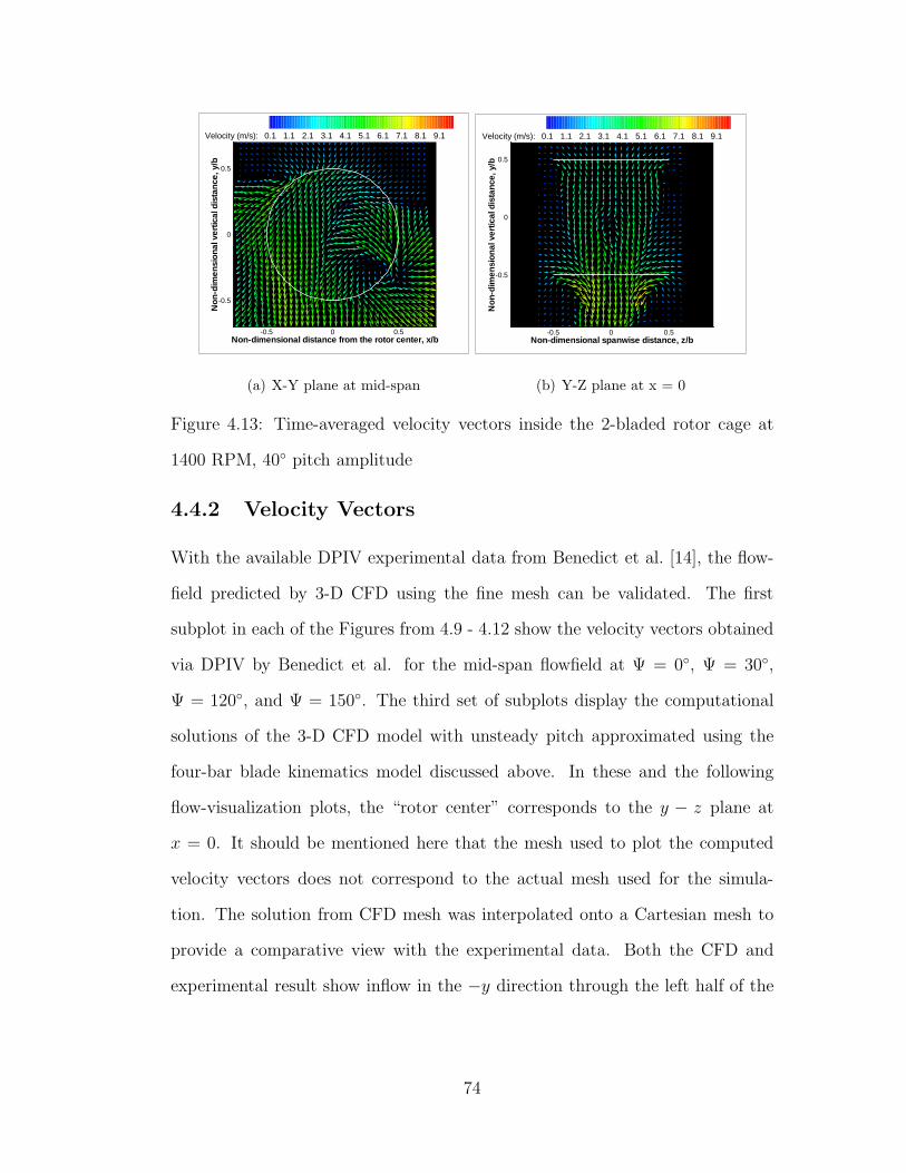
Non-dimensional distance from the rotor center, x/b

Non

-dim

ensi

onal

verti

cald

ista

nce,

y/b

-0.5 0 0.5

-0.5

0

0.5

Velocity (m/s): 0.1 1.1 2.1 3.1 4.1 5.1 6.1 7.1 8.1 9.1

(a) X-Y plane at mid-span

Non-dimensional spanwise distance, z/b

Non

-dim

ensi

onal

verti

cald

ista

nce,

y/b

-0.5 0 0.5

-0.5

0

0.5

Velocity (m/s): 0.1 1.1 2.1 3.1 4.1 5.1 6.1 7.1 8.1 9.1

(b) Y-Z plane at x = 0

Figure 4.13: Time-averaged velocity vectors inside the 2-bladed rotor cage at

1400 RPM, 40◦ pitch amplitude

4.4.2 Velocity Vectors

With the available DPIV experimental data from Benedict et al. [14], the flow-

field predicted by 3-D CFD using the fine mesh can be validated. The first

subplot in each of the Figures from 4.9 - 4.12 show the velocity vectors obtained

via DPIV by Benedict et al. for the mid-span flowfield at Ψ = 0◦, Ψ = 30◦,

Ψ = 120◦, and Ψ = 150◦. The third set of subplots display the computational

solutions of the 3-D CFD model with unsteady pitch approximated using the

four-bar blade kinematics model discussed above. In these and the following

flow-visualization plots, the “rotor center” corresponds to the y − z plane at

x = 0. It should be mentioned here that the mesh used to plot the computed

velocity vectors does not correspond to the actual mesh used for the simula-

tion. The solution from CFD mesh was interpolated onto a Cartesian mesh to

provide a comparative view with the experimental data. Both the CFD and

experimental result show inflow in the −y direction through the left half of the

74

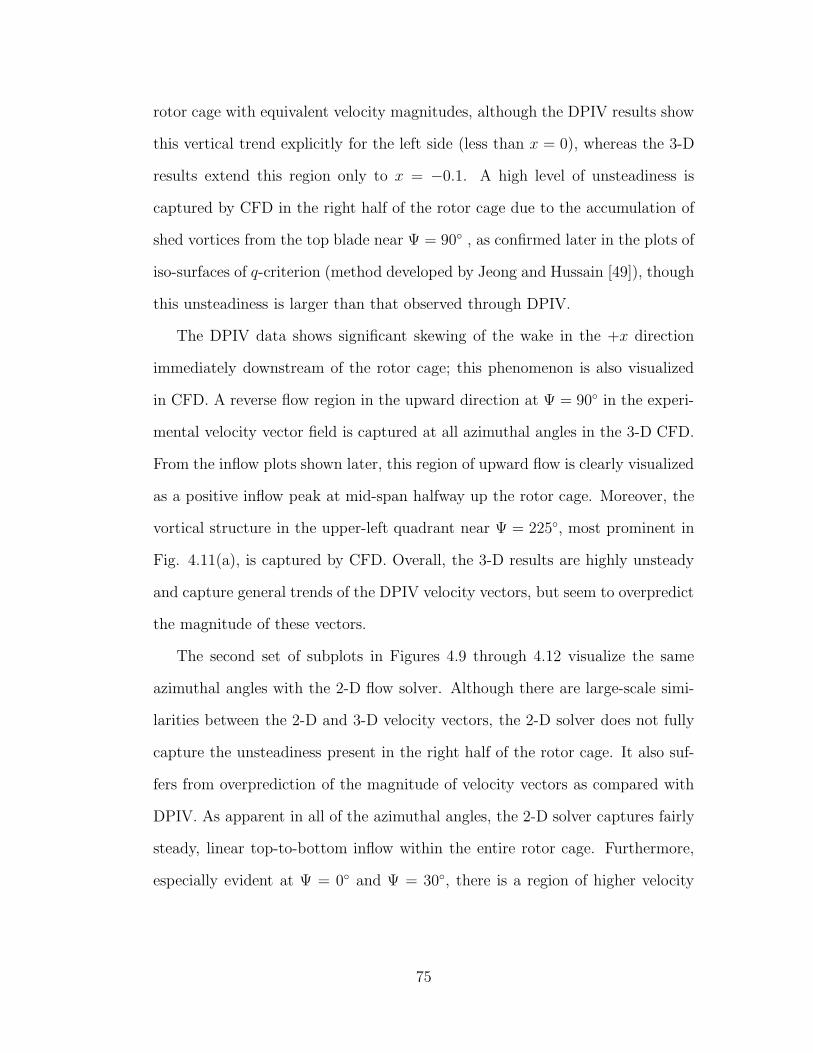
rotor cage with equivalent velocity magnitudes, although the DPIV results show

this vertical trend explicitly for the left side (less than x = 0), whereas the 3-D

results extend this region only to x = −0.1. A high level of unsteadiness is

captured by CFD in the right half of the rotor cage due to the accumulation of

shed vortices from the top blade near Ψ = 90◦ , as confirmed later in the plots of

iso-surfaces of q-criterion (method developed by Jeong and Hussain [49]), though

this unsteadiness is larger than that observed through DPIV.

The DPIV data shows significant skewing of the wake in the +x direction

immediately downstream of the rotor cage; this phenomenon is also visualized

in CFD. A reverse flow region in the upward direction at Ψ = 90◦ in the experi-

mental velocity vector field is captured at all azimuthal angles in the 3-D CFD.

From the inflow plots shown later, this region of upward flow is clearly visualized

as a positive inflow peak at mid-span halfway up the rotor cage. Moreover, the

vortical structure in the upper-left quadrant near Ψ = 225◦, most prominent in

Fig. 4.11(a), is captured by CFD. Overall, the 3-D results are highly unsteady

and capture general trends of the DPIV velocity vectors, but seem to overpredict

the magnitude of these vectors.

The second set of subplots in Figures 4.9 through 4.12 visualize the same

azimuthal angles with the 2-D flow solver. Although there are large-scale simi-

larities between the 2-D and 3-D velocity vectors, the 2-D solver does not fully

capture the unsteadiness present in the right half of the rotor cage. It also suf-

fers from overprediction of the magnitude of velocity vectors as compared with

DPIV. As apparent in all of the azimuthal angles, the 2-D solver captures fairly

steady, linear top-to-bottom inflow within the entire rotor cage. Furthermore,

especially evident at Ψ = 0◦ and Ψ = 30◦, there is a region of higher velocity

75

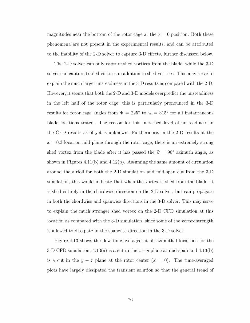
magnitudes near the bottom of the rotor cage at the x = 0 position. Both these

phenomena are not present in the experimental results, and can be attributed

to the inability of the 2-D solver to capture 3-D effects, further discussed below.

The 2-D solver can only capture shed vortices from the blade, while the 3-D

solver can capture trailed vortices in addition to shed vortices. This may serve to

explain the much larger unsteadiness in the 3-D results as compared with the 2-D.

However, it seems that both the 2-D and 3-D models overpredict the unsteadiness

in the left half of the rotor cage; this is particularly pronounced in the 3-D

results for rotor cage angles from Ψ = 225◦ to Ψ = 315◦ for all instantaneous

blade locations tested. The reason for this increased level of unsteadiness in

the CFD results as of yet is unknown. Furthermore, in the 2-D results at the

x = 0.3 location mid-plane through the rotor cage, there is an extremely strong

shed vortex from the blade after it has passed the Ψ = 90◦ azimuth angle, as

shown in Figures 4.11(b) and 4.12(b). Assuming the same amount of circulation

around the airfoil for both the 2-D simulation and mid-span cut from the 3-D

simulation, this would indicate that when the vortex is shed from the blade, it

is shed entirely in the chordwise direction on the 2-D solver, but can propagate

in both the chordwise and spanwise directions in the 3-D solver. This may serve

to explain the much stronger shed vortex on the 2-D CFD simulation at this

location as compared with the 3-D simulation, since some of the vortex strength

is allowed to dissipate in the spanwise direction in the 3-D solver.

Figure 4.13 shows the flow time-averaged at all azimuthal locations for the

3-D CFD simulation; 4.13(a) is a cut in the x− y plane at mid-span and 4.13(b)

is a cut in the y − z plane at the rotor center (x = 0). The time-averaged

plots have largely dissipated the transient solution so that the general trend of

76

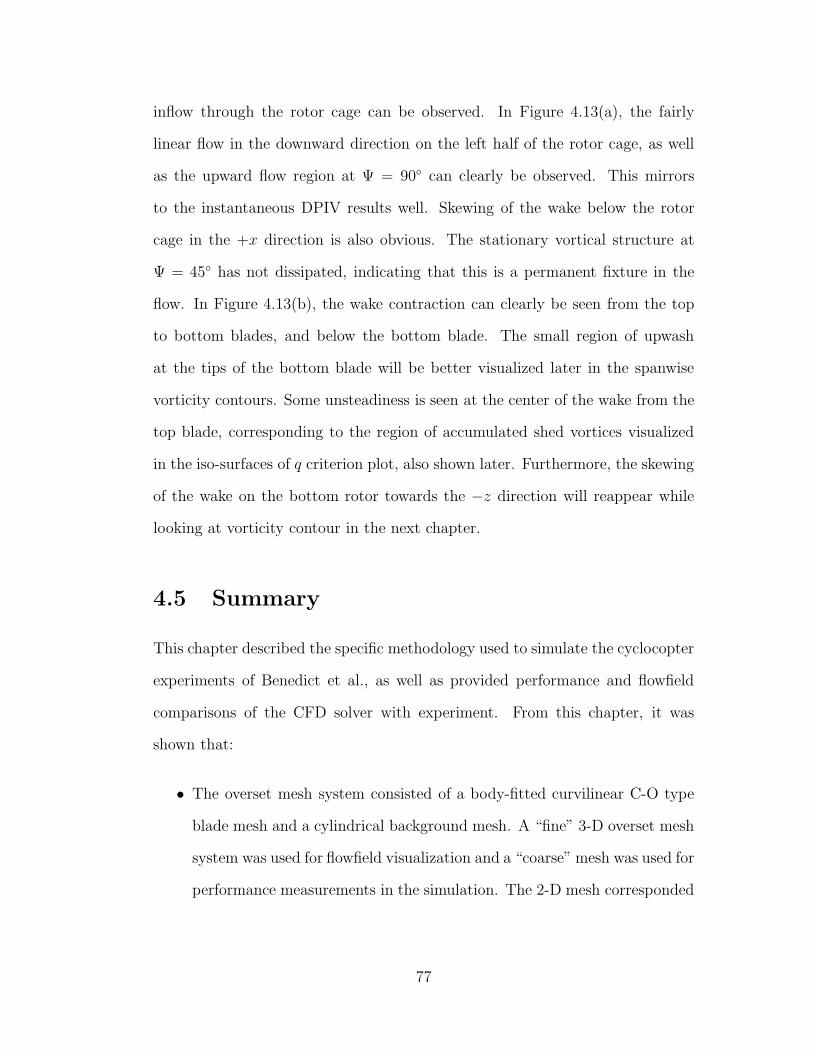
inflow through the rotor cage can be observed. In Figure 4.13(a), the fairly

linear flow in the downward direction on the left half of the rotor cage, as well

as the upward flow region at Ψ = 90◦ can clearly be observed. This mirrors

to the instantaneous DPIV results well. Skewing of the wake below the rotor

cage in the +x direction is also obvious. The stationary vortical structure at

Ψ = 45◦ has not dissipated, indicating that this is a permanent fixture in the

flow. In Figure 4.13(b), the wake contraction can clearly be seen from the top

to bottom blades, and below the bottom blade. The small region of upwash

at the tips of the bottom blade will be better visualized later in the spanwise

vorticity contours. Some unsteadiness is seen at the center of the wake from the

top blade, corresponding to the region of accumulated shed vortices visualized

in the iso-surfaces of q criterion plot, also shown later. Furthermore, the skewing

of the wake on the bottom rotor towards the −z direction will reappear while

looking at vorticity contour in the next chapter.

4.5 Summary

This chapter described the specific methodology used to simulate the cyclocopter

experiments of Benedict et al., as well as provided performance and flowfield

comparisons of the CFD solver with experiment. From this chapter, it was

shown that:

• The overset mesh system consisted of a body-fitted curvilinear C-O type

blade mesh and a cylindrical background mesh. A “fine” 3-D overset mesh

system was used for flowfield visualization and a “coarse” mesh was used for

performance measurements in the simulation. The 2-D mesh corresponded

77

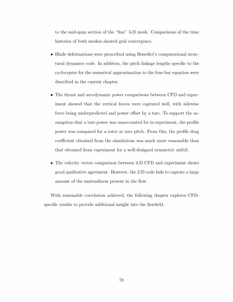
to the mid-span section of the “fine” 3-D mesh. Comparisons of the time

histories of both meshes showed grid convergence.

• Blade deformations were prescribed using Benedict’s computational struc-

tural dynamics code. In addition, the pitch linkage lengths specific to the

cyclocopter for the numerical approximation to the four-bar equation were

described in the current chapter.

• The thrust and aerodynamic power comparisons between CFD and exper-

iment showed that the vertical forces were captured well, with sidewise

force being underpredicted and power offset by a tare. To support the as-

sumption that a tare power was unaccounted for in experiment, the profile

power was compared for a rotor at zero pitch. From this, the profile drag

coefficient obtained from the simulations was much more reasonable than

that obtained from experiment for a well-designed symmetric airfoil.

• The velocity vector comparison between 3-D CFD and experiment shows

good qualitative agreement. However, the 2-D code fails to capture a large

amount of the unsteadiness present in the flow.

With reasonable correlation achieved, the following chapter explores CFD-

specific results to provide additional insight into the flowfield.

78

Chapter 5

CFD Predictions

Chapter 4 compared the flow solver predictions to the performance results ob-

tained from experiment. It was shown that vertical thrust was well-predicted,

while sidewise thrust was less-well predicted and, though the trend was captured

for aerodynamic power, the value of the prediction was offset by a tare factor.

This overall asserts reasonable correlation with experiment. In addition, the

qualitative comparisons of the flowfield with the PIV results showed that both

the 2-D and 3-D models obtained fairly good results. Taking this into consider-

ation, the following sections qualitatively explore characteristics of the flowfield

in ways difficult or impossible to obtain from experiment. It also seeks to ex-

plain the discrepancies between CFD performance predictions and experiment

through investigations of time-varying quantities within the flowfield. With the

validations performed in the previous section, the following predicted solutions

can be taken to exhibit reasonable physical accuracy.

79

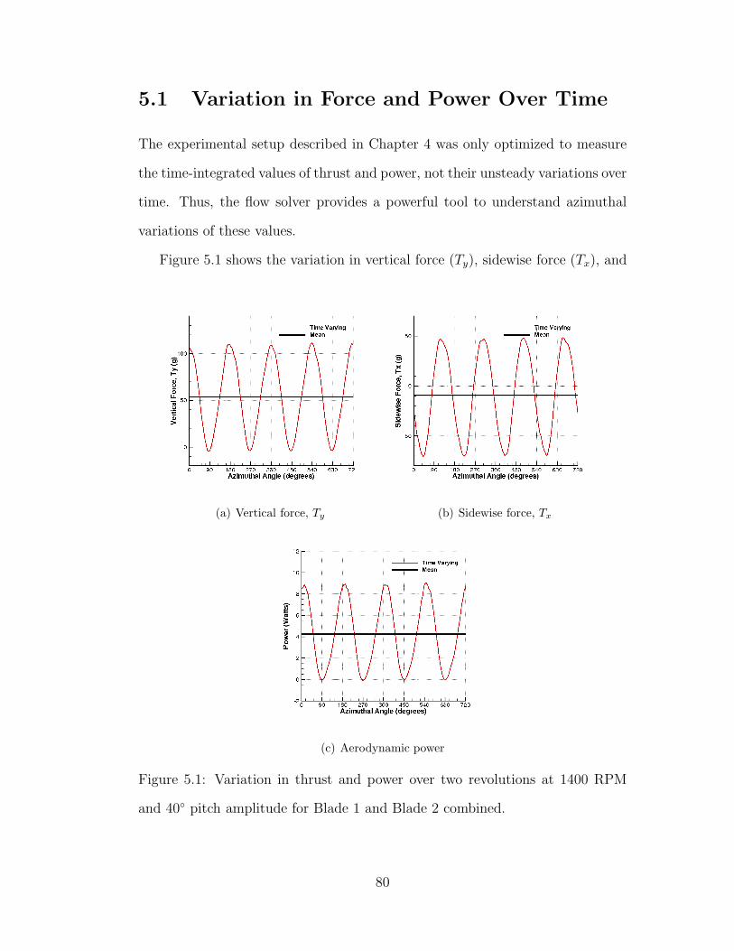
5.1 Variation in Force and Power Over Time

The experimental setup described in Chapter 4 was only optimized to measure

the time-integrated values of thrust and power, not their unsteady variations over

time. Thus, the flow solver provides a powerful tool to understand azimuthal

variations of these values.

Figure 5.1 shows the variation in vertical force (Ty), sidewise force (Tx), and

(a) Vertical force, Ty (b) Sidewise force, Tx

(c) Aerodynamic power

Figure 5.1: Variation in thrust and power over two revolutions at 1400 RPM

and 40◦ pitch amplitude for Blade 1 and Blade 2 combined.

80

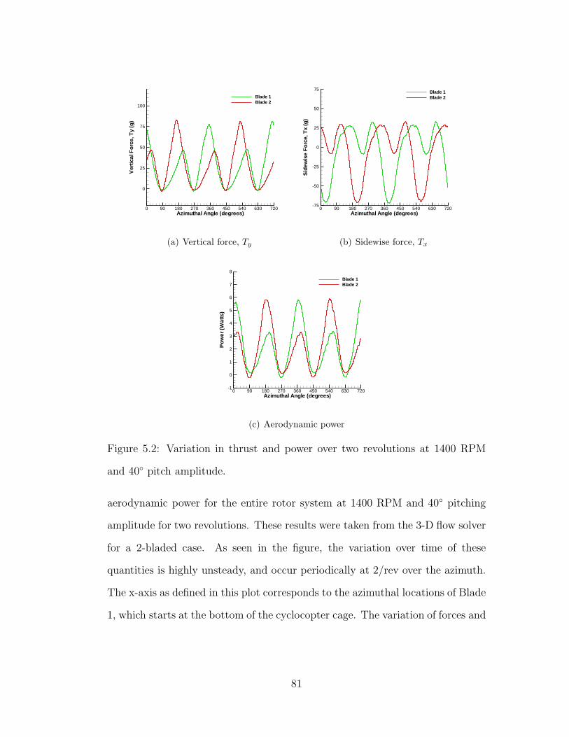
Azimuthal Angle (degrees)

Ver

tical

For

ce,T

y(g

)

0 90 180 270 360 450 540 630 720

0

25

50

75

100

Blade 1Blade 2

(a) Vertical force, Ty

Azimuthal Angle (degrees)

Sid

ewis

eF

orce

,Tx

(g)

0 90 180 270 360 450 540 630 720-75

-50

-25

0

25

50

75Blade 1Blade 2

(b) Sidewise force, Tx

Azimuthal Angle (degrees)

Pow

er(W

atts

)

0 90 180 270 360 450 540 630 720-1

0

1

2

3

4

5

6

7

8

Blade 1Blade 2

(c) Aerodynamic power

Figure 5.2: Variation in thrust and power over two revolutions at 1400 RPM

and 40◦ pitch amplitude.

aerodynamic power for the entire rotor system at 1400 RPM and 40◦ pitching

amplitude for two revolutions. These results were taken from the 3-D flow solver

for a 2-bladed case. As seen in the figure, the variation over time of these

quantities is highly unsteady, and occur periodically at 2/rev over the azimuth.

The x-axis as defined in this plot corresponds to the azimuthal locations of Blade

1, which starts at the bottom of the cyclocopter cage. The variation of forces and

81

power in revolution two (360◦ < Ψ < 720◦) is highly similar to revolution one,

(0◦ < Ψ < 360◦), thus reinforcing the assertion that periodicity was attained in

the unsteady flow solution. The RMS values obtained for the time histories of

Tx, Ty, and power are 21.56 grams, 34.34 grams, and 2.77 Watts respectively.

All of the RMS values are significantly high (on the same order or higher than

mean values), signifying a large amount of fluctuation from the mean value.

While CFD can be employed to observe the fluctuations in thrust and power

over the entire rotor, the solution can also be decomposed into the timewise

variations of these quantities over each blade, as seen in Figure 5.2. At zero az-

imuthal angle (Ψ = 0◦) in the plot, Blade 1 is at the lowest y-axis position, while

Blade 2 is opposite Blade 1 at the highest y-axis position. Periodicity is clearly

evidenced via the trends in the solution from each blade: the force and power

values for Blade 2 look almost identical to Blade 1 but phase shifted by 180◦,

and also from one revolution to another if only one blade is considered. The plot

clearly shows large variation in all the integrated values; whereas the variation

in thrusts over the entire rotor was relatively sinusoidal, the thrusts over each

individual blade show highly different trends. Analysis of these trends, as un-

dertaken in the following two sections, disclose details about blade performance

at various azimuthal locations in the cyclocopter cage.

5.1.1 Vertical Force and Aerodynamic Power Variation

over Time

From Figure 5.2(a), one can observe that the maximum vertical force and aero-

dynamic power is attained when the blade is at the lowest azimuthal position,

i.e. when the blade is at the bottom of the cyclocopter cage. This is counter-

82

intuitive, as intuition states that the inflow produced by the top of the rotor cage

would decrease the angle of attack of the bottom half of the cage, and therefore

one would expect the largest values to be attained at the top. Further, if we

consider that at the instant in time when the airfoils are opposite each other at

Ψ = 0◦ and Ψ = 180◦ that the blades can be thought of as two actuator disks,

momentum theory models of coaxial rotors [50] state that since the lower rotor

operates in the slipstream of the upper rotor, for a given value of thrust its net

induced velocity is higher and hence its net efficiency is lower. Though the lower

rotor is seeing a greater inflow velocity over half its disk area due to the down-

wash from the top rotor, the complexity of the rotor flowfield and interaction

between the vortices shed by the top rotor on the lower rotor blades cause an

overall loss in efficiency on the lower disk. Thus, following this logic, one would

expect that the lower blade of the cyclocopter produces less lift; however, this

is contradicted by the time-varying results. As will be discussed later in Section

5.1.4, the trends observed from CFD are attributed to the virtual camber effect.

The timewise variation in aerodynamic power is similar to the vertical force

time history. However, maximum aerodynamic power is achieved simultaneously

by the upper and lower blades at the maximum positive and negative y-axis

directions. This is different from Ty, where the maximum vertical force of the

upper blade is phase-shifted about +30◦ relative to the lower blade.

5.1.2 Sidewise Force Variation over Time

The time history plot of sidewise force shows large unsteady variations due to

the pitching motion of the cyclocopter. As shown in Figure 5.2(b), the peak

amplitude of instantaneous sidewise force is up to 15 times the mean value ob-

83

tained for Figure 4.7. Therefore, this signifies that the mean value of sidewise

force is extremely sensitive to changes in blade pitch or deformation. A small

error in the blade pitch or deformation from experiment can directly result in

small changes to the time history of the sidewise force. These small variations

can, in turn, lead to significant changes in the mean sidewise force. Therefore,

performance in the sidewise direction is very difficult to predict with CFD.

5.1.3 Comparison Between Deformed and Undeformed

Blades

As discussed in Section 2.3.3, radial bending, tangential bending, and torsional

blade deformations obtained from Benedict’s structural dynamic code were pre-

scribed into TURNS. A comparison of the force generated by the undeformed

blades and blades with prescribed deformations for a 2-bladed cyclocopter op-

erating at 1400 RPM, 40◦ pitch amplitude is given in Figure 5.3. As seen in the

figure, over two revolutions there is very little difference between inclusion and

negation of structural deflections in the numerical simulation. The deformed

blades generally attain a higher vertical force peak and a lower +y sidewise force

peak, but these differences are to within 14% of the undeformed model for all

quantities calculated. Hence, it is largely unnecessary to prescribe blade de-

formations for the cyclocopter for this configuration, since the blades are fairly

rigid and the RPM is low. For more flexible blades at higher RPMs, however,

the structural deformations cannot be as easily neglected.

84

Azimuthal Angle (Degrees)

Ver

tical

For

ce,T

y(g

)

0 90 180 270 360 450 540 630 720-25

0

25

50

75

100

No deformationWith deformation

(a) Vertical force, Ty

Azimuthal Angle (Degrees)

Sid

ewis

eF

orce

,-T

x(g

)

0 90 180 270 360 450 540 630 720-100

-75

-50

-25

0

25

50

75

No deformationWith deformation

(b) Sidewise force, Tx

Figure 5.3: Comparison between deformed and undeformed blades over two

revolutions at 1400 RPM and 40◦ pitch amplitude for Blade 1.

5.1.4 Cambered Airfoil Analysis

As discussed in Section 5.1.1, the discrepancy in vertical thrust and power

obtained in the unsteady time history at the “bottom” (Ψ = 0◦) or “top”

(Ψ = 180◦) location on the rotor cage is due to the virtual camber effect. The

virtual camber effect was first noticed by the vertical axis wind turbine commu-

nity, but more recently for cyclocopter MAVs by Yun et al. [17] and Benedict et

al. [16]. In the cycloidal rotor, since the blades travel on a circular path about

the cage, and the ratio of chord length to radius of the circle is relatively large,

the symmetric airfoil shown in 5.4(a) will not see the same angles of attack along

the chord at zero pitch. At any instant, the leading edge will experience a nega-

tive angle of attack; the pitching axis (at quarter-chord for the cyclocopter) will

have no angle of attack with respect to the freestream; and increasing chord-

wise positions from the pitching axis towards the trailing edge will experience

increasingly positive angles of attack; this corresponds effectively to a cambered

85

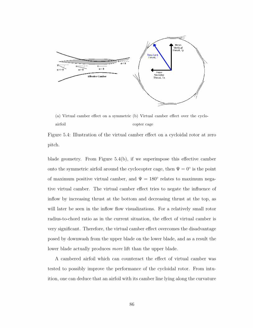
(a) Virtual camber effect on a symmetric

airfoil

(b) Virtual camber effect over the cyclo-

copter cage

Figure 5.4: Illustration of the virtual camber effect on a cycloidal rotor at zero

pitch.

blade geometry. From Figure 5.4(b), if we superimpose this effective camber

onto the symmetric airfoil around the cyclocopter cage, then Ψ = 0◦ is the point

of maximum positive virtual camber, and Ψ = 180◦ relates to maximum nega-

tive virtual camber. The virtual camber effect tries to negate the influence of

inflow by increasing thrust at the bottom and decreasing thrust at the top, as

will later be seen in the inflow flow visualizations. For a relatively small rotor

radius-to-chord ratio as in the current situation, the effect of virtual camber is

very significant. Therefore, the virtual camber effect overcomes the disadvantage

posed by downwash from the upper blade on the lower blade, and as a result the

lower blade actually produces more lift than the upper blade.

A cambered airfoil which can counteract the effect of virtual camber was

tested to possibly improve the performance of the cycloidal rotor. From intu-

ition, one can deduce that an airfoil with its camber line lying along the curvature

86

(a) NACA 0010 profile superimposed on

4.5% camber line.

(b) Cambered airfoil placement inside the

rotor cage

Figure 5.5: Cambered airfoil design to negate the virtual camber effect.

of the cage should have no virtual camber effect at zero pitch. Such an airfoil

may not be able to completely negate the virtual camber effect when the blade is

at non-zero pitch, but it still can counteract most of its effect. Using this logic,

with regard to dimensions of the current experimental setup, the cambered airfoil

that needs to be used should have 4.5% camber. To obtain a comparative perfor-

mance with the symmetric NACA 0010 run, an airfoil geometry is constructed

by superimposing the thickness of the NACA 0010 profile onto the 4.5% circular

arc camber line. Then, it is placed in the cyclocopter cage with camber pointed

inward towards the center; a schematic of the airfoil and its placement inside

the rotor cage is shown in Figure 5.5. Performance calculation for this cambered

airfoil is done for 40◦ pitch amplitude 2-bladed case operating at 1400 RPM.

Figure 5.6 shows the comparison between one blade of the cambered airfoil

geometry and the symmetric NACA 0010 airfoil for vertical force, sidewise force,

and power. The time history of the vertical force clearly shows that use of the

87

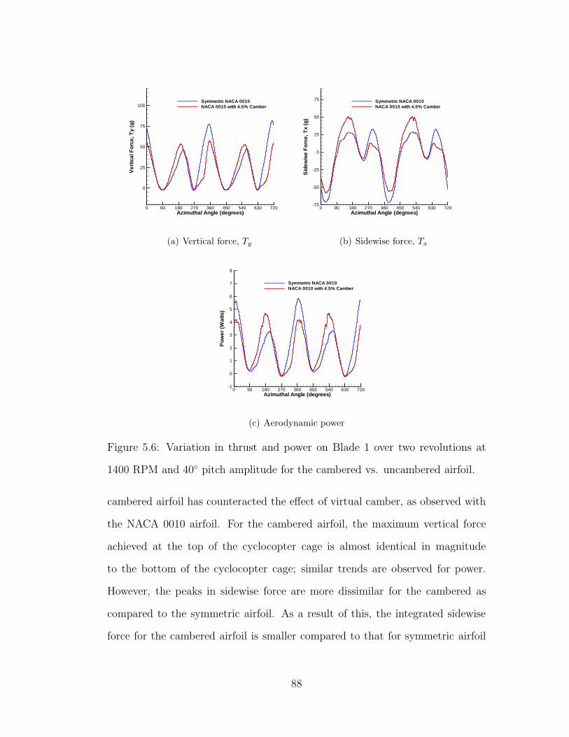
Azimuthal Angle (degrees)

Ver

tical

For

ce,T

y(g

)

0 90 180 270 360 450 540 630 720

0

25

50

75

100Symmetric NACA 0010NACA 0010 with 4.5% Camber

(a) Vertical force, Ty

Azimuthal Angle (degrees)

Sid

ewis

eF

orce

,Tx

(g)

0 90 180 270 360 450 540 630 720-75

-50

-25

0

25

50

75 Symmetric NACA 0010NACA 0010 with 4.5% Camber

(b) Sidewise force, Tx

Azimuthal Angle (degrees)

Pow

er(W

atts

)

0 90 180 270 360 450 540 630 720-1

0

1

2

3

4

5

6

7

8

Symmetric NACA 0010NACA 0010 with 4.5% Camber

(c) Aerodynamic power

Figure 5.6: Variation in thrust and power on Blade 1 over two revolutions at

1400 RPM and 40◦ pitch amplitude for the cambered vs. uncambered airfoil.

cambered airfoil has counteracted the effect of virtual camber, as observed with

the NACA 0010 airfoil. For the cambered airfoil, the maximum vertical force

achieved at the top of the cyclocopter cage is almost identical in magnitude

to the bottom of the cyclocopter cage; similar trends are observed for power.

However, the peaks in sidewise force are more dissimilar for the cambered as

compared to the symmetric airfoil. As a result of this, the integrated sidewise

force for the cambered airfoil is smaller compared to that for symmetric airfoil

88

(−2.58 grams compared to −9.12 grams).

Considering the integrated values of the vertical force and power for the

cycloidal rotor using a cambered airfoil, it is seen that although the these values

become relatively similar at the top and bottom of the rotor cage, the combined

maximum thrust achieved with the cambered configuration is not as high as the

symmetric. The mean Ty and power for the cambered airfoil are 44.69 grams and

3.93 Watts; the analogous values for the symmetric airfoil are 53.75 grams and

4.23 Watts, respectively. For the purpose of performance comparison, the power

required by the symmetric airfoil is calculated at the thrust produced by the

cambered airfoil by interpolating data from Figs. 4.8(a) and (c). Interpolated

power for the symmetric airfoil was found to be 3.6 Watts, which is slightly lower

than the power for cambered airfoil. Therefore, camber seems to have a slight

detrimental effect on the performance. However, a clear conclusion cannot be

made on the effect of camber by merely a single performance result. Cambered

blades might offer beneficial results at higher pitch angle, as the blades now will

have reduced stall due to the reduction in lift peak. Further investigations must

be undertaken to ascertain the full effect of using the cambered airfoils.

5.2 Spanwise Thrust Distribution

To gain insight into the three-dimensionality of the flowfield, the spanwise distri-

bution of vertical and sidewise thrust was examined as a function of azimuthal

angle. The 3-D CFD simulation results at 1400RPM and 40◦ pitch amplitude

with the fine mesh are shown in Figures 5.7 and 5.8. In these plots, the z-axis

has been non-dimensionalized with respect to the rotor span, b; this convention

applies to all the axes in the ensuing flowfield visualization plots. Also, at any

89

instant in the revolution, the azimuthal angle of the top blade is always 180◦ out

of phase with respect to the bottom blade.

The spanwise distribution of vertical and sidewise thrust show significant

changes over the span at most azimuthal locations. Three main phenomena

which cause variation of these quantities along the span are described below:

• The tip vortex generated near the ends of the blade cause a local peaking

of the thrusts before it drops down to zero at the tip.

• Unsteady shedding causes fluctuations to the distribution near the mid-

span sections of the blade, most apparent for Blade 1 at the 30◦ and 60◦

azimuth locations in part (b) and (c) of the spanwise distribution plots.

• Different inflow velocities due to wake contraction from one blade cause

the mid-portion of the other blade to produce significantly higher or lower

thrust compared to its outer portion. This variation is seen at almost all

the wake-ages on both the force distributions, but most prominently in the

sidewise force distribution when the blade is at the right most part of the

cage, ΨB1 = 90◦. In this plot, there is a clear demarcation between the

higher thrust region at −0.25 < z/b < 0.25, and lower thrust outer regions

−0.5 < z/b < −0.25 and 0.25 < z/b < 0.5.

For further exploration into the third phenomenon described above, the

instantaneous inflow normalized by rotational speed has been plotted for the

quarter-chord line along the span, as shown in Figure 5.9. From the plot, it can

be seen that at all azimuth locations other than the locations from 60◦ to 120◦

azimuth, there is a downwash across the span of the rotor. At 60◦ to 120◦ az-

imuth locations, the inflow acts in the upward direction. Note that, this upward

90

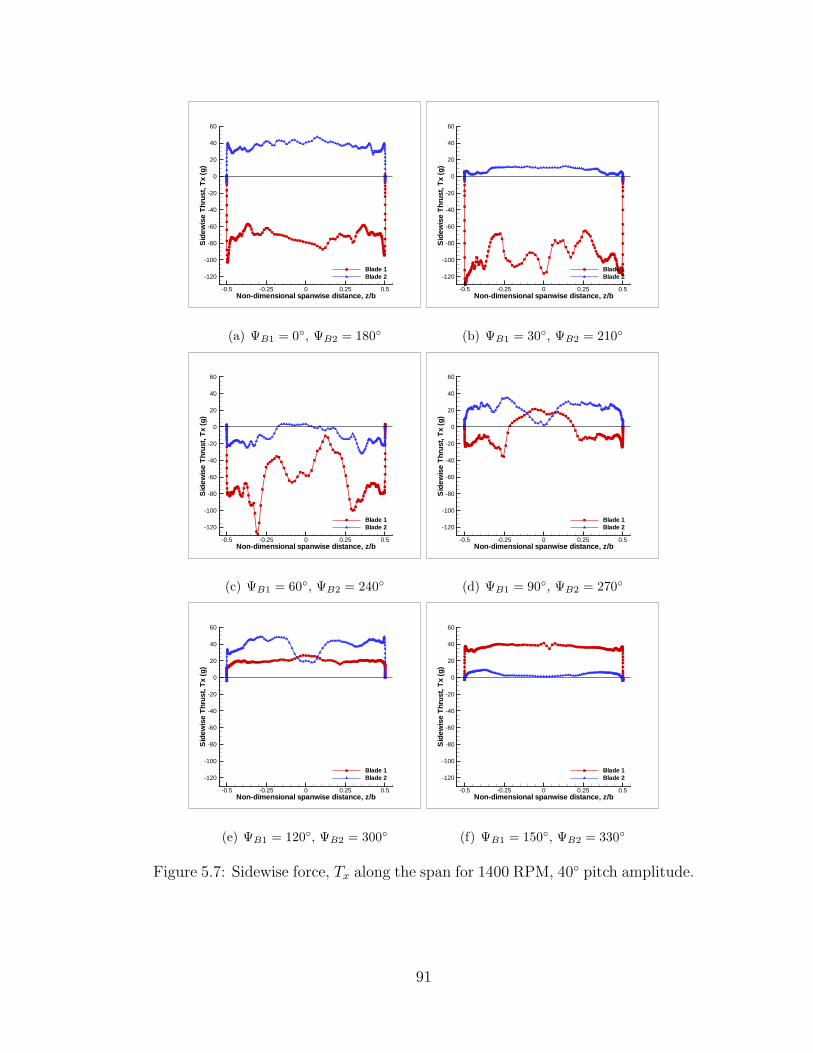
Non-dimensional spanwise distance, z/b

Sid

ewis

eT

hrus

t,T

x(g

)

-0.5 -0.25 0 0.25 0.5

-120

-100

-80

-60

-40

-20

0

20

40

60

Blade 1Blade 2

(a) ΨB1 = 0◦, ΨB2 = 180◦

Non-dimensional spanwise distance, z/b

Sid

ewis

eT

hrus

t,T

x(g

)

-0.5 -0.25 0 0.25 0.5

-120

-100

-80

-60

-40

-20

0

20

40

60

Blade 1Blade 2

(b) ΨB1 = 30◦, ΨB2 = 210◦

Non-dimensional spanwise distance, z/b

Sid

ewis

eT

hrus

t,T

x(g

)

-0.5 -0.25 0 0.25 0.5

-120

-100

-80

-60

-40

-20

0

20

40

60

Blade 1Blade 2

(c) ΨB1 = 60◦, ΨB2 = 240◦

Non-dimensional spanwise distance, z/b

Sid

ewis

eT

hrus

t,T

x(g

)

-0.5 -0.25 0 0.25 0.5

-120

-100

-80

-60

-40

-20

0

20

40

60

Blade 1Blade 2

(d) ΨB1 = 90◦, ΨB2 = 270◦

Non-dimensional spanwise distance, z/b

Sid

ewis

eT

hrus

t,T

x(g

)

-0.5 -0.25 0 0.25 0.5

-120

-100

-80

-60

-40

-20

0

20

40

60

Blade 1Blade 2

(e) ΨB1 = 120◦, ΨB2 = 300◦

Non-dimensional spanwise distance, z/b

Sid

ewis

eT

hrus

t,T

x(g

)

-0.5 -0.25 0 0.25 0.5

-120

-100

-80

-60

-40

-20

0

20

40

60

Blade 1Blade 2

(f) ΨB1 = 150◦, ΨB2 = 330◦

Figure 5.7: Sidewise force, Tx along the span for 1400 RPM, 40◦ pitch amplitude.

91

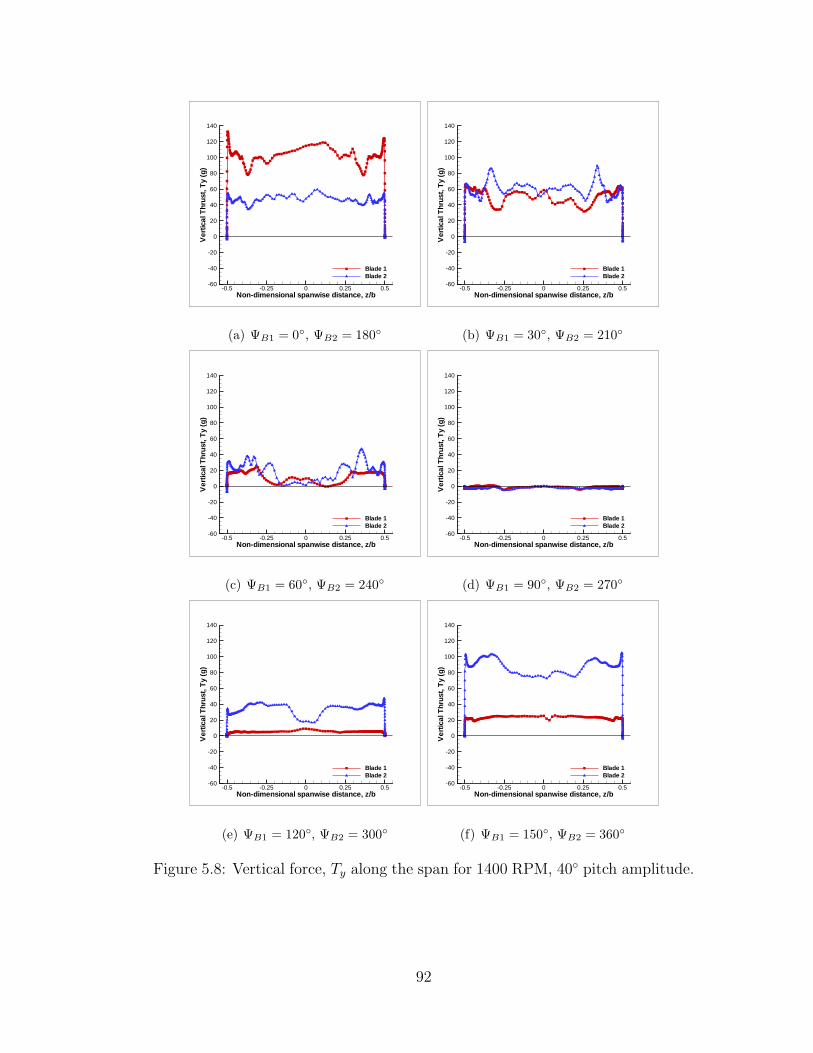
Non-dimensional spanwise distance, z/b

Ver

tical

Thr

ust,

Ty

(g)

-0.5 -0.25 0 0.25 0.5-60

-40

-20

0

20

40

60

80

100

120

140

Blade 1Blade 2

(a) ΨB1 = 0◦, ΨB2 = 180◦

Non-dimensional spanwise distance, z/b

Ver

tical

Thr

ust,

Ty

(g)

-0.5 -0.25 0 0.25 0.5-60

-40

-20

0

20

40

60

80

100

120

140

Blade 1Blade 2

(b) ΨB1 = 30◦, ΨB2 = 210◦

Non-dimensional spanwise distance, z/b

Ver

tical

Thr

ust,

Ty

(g)

-0.5 -0.25 0 0.25 0.5-60

-40

-20

0

20

40

60

80

100

120

140

Blade 1Blade 2

(c) ΨB1 = 60◦, ΨB2 = 240◦

Non-dimensional spanwise distance, z/b

Ver

tical

Thr

ust,

Ty

(g)

-0.5 -0.25 0 0.25 0.5-60

-40

-20

0

20

40

60

80

100

120

140

Blade 1Blade 2

(d) ΨB1 = 90◦, ΨB2 = 270◦

Non-dimensional spanwise distance, z/b

Ver

tical

Thr

ust,

Ty

(g)

-0.5 -0.25 0 0.25 0.5-60

-40

-20

0

20

40

60

80

100

120

140

Blade 1Blade 2

(e) ΨB1 = 120◦, ΨB2 = 300◦

Non-dimensional spanwise distance, z/b

Ver

tical

Thr

ust,

Ty

(g)

-0.5 -0.25 0 0.25 0.5-60

-40

-20

0

20

40

60

80

100

120

140

Blade 1Blade 2

(f) ΨB1 = 150◦, ΨB2 = 360◦

Figure 5.8: Vertical force, Ty along the span for 1400 RPM, 40◦ pitch amplitude.

92

flow region was observed in both CFD and experimental velocity vector plots

shown earlier. The important feature to notice from these plots is that the inflow

at all azimuth locations has higher absolute value around the mid-sections of the

blade, and almost linearly drops down to zero towards the tip. The extent of this

high inflow mid-section region varies with azimuthal location and is determined

by the amount of wake contraction at that location. When observed carefully, it

can be noticed that the spanwise thrust distribution plots clearly correlate well

with the inflow plots at most of the azimuth locations. As expected, the inflow

velocities acting downward (negative value) are seen to decrease the thrust and

the velocities acting upwards (positive value) increase the thrust.

Overall, from the plots presented in this section, it is observed that there

is significant variation in the spanwise thrust distribution, attesting to the high

level of three-dimensionality in the flowfield. Thus, although good performance

predictions were obtained using 2D CFD calculations, a 3D calculation is essen-

tial to understand the details of the flow physics.

5.3 Time-Averaged Inflow Distribution

Inflow distribution, as was shown in the previous section, is largely related to

the spanwise thrust, and thus can provide a good precept to characterize the

thrust distribution over the blade at a given azimuthal position. Furthermore,

inflow can also prove a useful tool to visualize the flow velocities over the entire

rotor system.

Figure 5.10 shows surface plots of inflow normalized by rotational speed taken

at different cuts in the x − z plane along the y-axis. At y = +0.8R, the inflow

ratio is fairly small across the rotor, with the largest inflow being observed at

93

Non-dimensional spanwise distance, z/b

Inflo

wR

atio

-1 -0.5 0 0.5 1

-0.6

-0.5

-0.4

-0.3

-0.2

-0.1

0

0.1

0.2

0.3

0.4Blade 1Blade 2

(a) ΨB1 = 0◦, ΨB2 = 180◦

Non-dimensional spanwise distance, z/b

Inflo

wR

atio

-1 -0.5 0 0.5 1

-0.6

-0.5

-0.4

-0.3

-0.2

-0.1

0

0.1

0.2

0.3

0.4Blade 1Blade 2

(b) ΨB1 = 30◦, ΨB2 = 210◦

Non-dimensional spanwise distance, z/b

Inflo

wR

atio

-1 -0.5 0 0.5 1

-0.6

-0.5

-0.4

-0.3

-0.2

-0.1

0

0.1

0.2

0.3

0.4Blade 1Blade 2

(c) ΨB1 = 60◦, ΨB2 = 240◦

Non-dimensional spanwise distance, z/b

Inflo

wR

atio

-1 -0.5 0 0.5 1

-0.6

-0.5

-0.4

-0.3

-0.2

-0.1

0

0.1

0.2

0.3

0.4Blade 1Blade 2

(d) ΨB1 = 90◦, ΨB2 = 270◦

Non-dimensional spanwise distance, z/b

Inflo

wR

atio

-1 -0.5 0 0.5 1

-0.6

-0.5

-0.4

-0.3

-0.2

-0.1

0

0.1

0.2

0.3

0.4Blade 1Blade 2

(e) ΨB1 = 120◦, ΨB2 = 300◦

Non-dimensional spanwise distance, z/b

Inflo

wR

atio

-1 -0.5 0 0.5 1

-0.6

-0.5

-0.4

-0.3

-0.2

-0.1

0

0.1

0.2

0.3

0.4Blade 1Blade 2

(f) ΨB1 = 150◦, ΨB2 = 330◦

Figure 5.9: Inflow vs. spanwise location at the quarter-chord position of each

blade for 1400 RPM, 40◦ pitch amplitude.

94

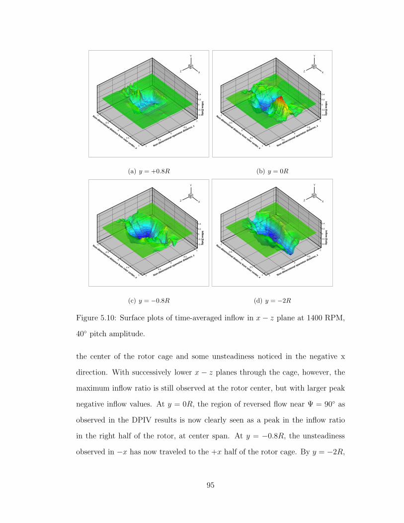
Non-dimensional distance fromrotor center, x

-1

-0.5

0

0.5

1

Inf lowR

atio

-0.4

-0.2

0

0.2

0.4

Non-dimensional spanwise distance , z

-1

-0.5

0

0.5

1

X

Y

Z

(a) y = +0.8R

Non-dimensional distance fromrotor center, x

-1

-0.5

0

0.5

1

Inflow

Ratio

-0.4

-0.2

0

0.2

0.4

Non-dimensional spanwise distance, z

-1

-0.5

0

0.5

1

X

Y

Z

(b) y = 0R

Non-dimensional distance fromrotor center, x

-1

-0.5

0

0.5

1

Inflow

Ratio

-0.4

-0.2

0

0.2

0.4

Non-dimensional spanwise distance, z

-1

-0.5

0

0.5

1

X

Y

Z

(c) y = −0.8R

Non-dimensional distance fromrotor center, x

-1

-0.5

0

0.5

1

Inflow

Ra

tio

-0.4

-0.2

0

0.2

0.4

Non-dimensional spanwise distance, z

-1

-0.5

0

0.5

1

X

Y

Z

(d) y = −2R

Figure 5.10: Surface plots of time-averaged inflow in x − z plane at 1400 RPM,

40◦ pitch amplitude.

the center of the rotor cage and some unsteadiness noticed in the negative x

direction. With successively lower x − z planes through the cage, however, the

maximum inflow ratio is still observed at the rotor center, but with larger peak

negative inflow values. At y = 0R, the region of reversed flow near Ψ = 90◦ as

observed in the DPIV results is now clearly seen as a peak in the inflow ratio

in the right half of the rotor, at center span. At y = −0.8R, the unsteadiness

observed in −x has now traveled to the +x half of the rotor cage. By y = −2R,

95

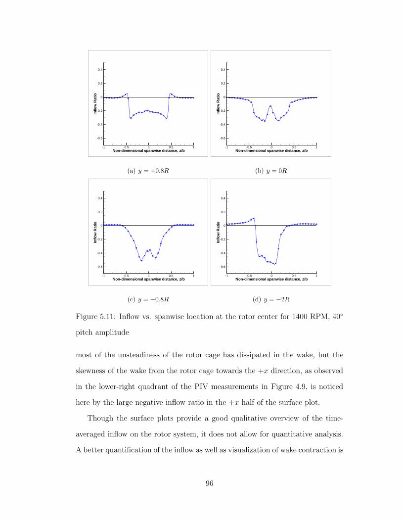
Non-dimensional spanwise distance, z/b

Inflo

wR

atio

-1 -0.5 0 0.5 1

-0.6

-0.4

-0.2

0

0.2

0.4

(a) y = +0.8R

Non-dimensional spanwise distance, z/b

Inflo

wR

atio

-1 -0.5 0 0.5 1

-0.6

-0.4

-0.2

0

0.2

0.4

(b) y = 0R

Non-dimensional spanwise distance, z/b

Inflo

wR

atio

-1 -0.5 0 0.5 1

-0.6

-0.4

-0.2

0

0.2

0.4

(c) y = −0.8R

Non-dimensional spanwise distance, z/b

Inflo

wR

atio

-1 -0.5 0 0.5 1

-0.6

-0.4

-0.2

0

0.2

0.4

(d) y = −2R

Figure 5.11: Inflow vs. spanwise location at the rotor center for 1400 RPM, 40◦

pitch amplitude

most of the unsteadiness of the rotor cage has dissipated in the wake, but the

skewness of the wake from the rotor cage towards the +x direction, as observed

in the lower-right quadrant of the PIV measurements in Figure 4.9, is noticed

here by the large negative inflow ratio in the +x half of the surface plot.

Though the surface plots provide a good qualitative overview of the time-

averaged inflow on the rotor system, it does not allow for quantitative analysis.

A better quantification of the inflow as well as visualization of wake contraction is

96

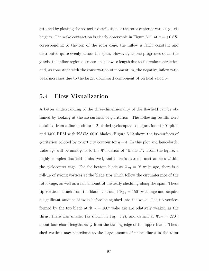
attained by plotting the spanwise distribution at the rotor center at various y-axis

heights. The wake contraction is clearly observable in Figure 5.11 at y = +0.8R,

corresponding to the top of the rotor cage, the inflow is fairly constant and

distributed quite evenly across the span. However, as one progresses down the

y-axis, the inflow region decreases in spanwise length due to the wake contraction

and, as consistent with the conservation of momentum, the negative inflow ratio

peak increases due to the larger downward component of vertical velocity.

5.4 Flow Visualization

A better understanding of the three-dimensionality of the flowfield can be ob-

tained by looking at the iso-surfaces of q-criterion. The following results were

obtained from a fine mesh for a 2-bladed cyclocopter configuration at 40◦ pitch

and 1400 RPM with NACA 0010 blades. Figure 5.12 shows the iso-surfaces of

q-criterion colored by x-vorticity contour for q = 4. In this plot and henceforth,

wake age will be analogous to the Ψ location of “Blade 1”. From the figure, a

highly complex flowfield is observed, and there is extreme unsteadiness within

the cyclocopter cage. For the bottom blade at ΨB1 = 0◦ wake age, there is a

roll-up of strong vortices at the blade tips which follow the circumference of the

rotor cage, as well as a fair amount of unsteady shedding along the span. These

tip vortices detach from the blade at around ΨB1 = 150◦ wake age and acquire

a significant amount of twist before being shed into the wake. The tip vortices

formed by the top blade at ΨB2 = 180◦ wake age are relatively weaker, as the

thrust there was smaller (as shown in Fig. 5.2), and detach at ΨB2 = 270◦,

about four chord lengths away from the trailing edge of the upper blade. These

shed vortices may contribute to the large amount of unsteadiness in the rotor

97

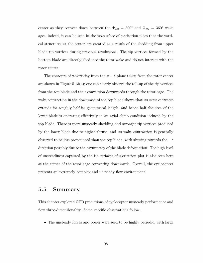
center as they convect down between the ΨB2 = 300◦ and ΨB2 = 360◦ wake

ages; indeed, it can be seen in the iso-surface of q-criterion plots that the vorti-

cal structures at the center are created as a result of the shedding from upper

blade tip vortices during previous revolutions. The tip vortices formed by the

bottom blade are directly shed into the rotor wake and do not interact with the

rotor center.

The contours of x-vorticity from the y − z plane taken from the rotor center

are shown in Figure 5.13(a); one can clearly observe the roll-up of the tip vortices

from the top blade and their convection downwards through the rotor cage. The

wake contraction in the downwash of the top blade shows that its vena contracta

extends for roughly half its geometrical length, and hence half the area of the

lower blade is operating effectively in an axial climb condition induced by the

top blade. There is more unsteady shedding and stronger tip vortices produced

by the lower blade due to higher thrust, and its wake contraction is generally

observed to be less pronounced than the top blade, with skewing towards the −z

direction possibly due to the asymmetry of the blade deformation. The high level

of unsteadiness captured by the iso-surfaces of q-criterion plot is also seen here

at the center of the rotor cage convecting downwards. Overall, the cyclocopter

presents an extremely complex and unsteady flow environment.

5.5 Summary

This chapter explored CFD predictions of cyclocopter unsteady performance and

flow three-dimensionality. Some specific observations follow:

• The unsteady forces and power were seen to be highly periodic, with large

98

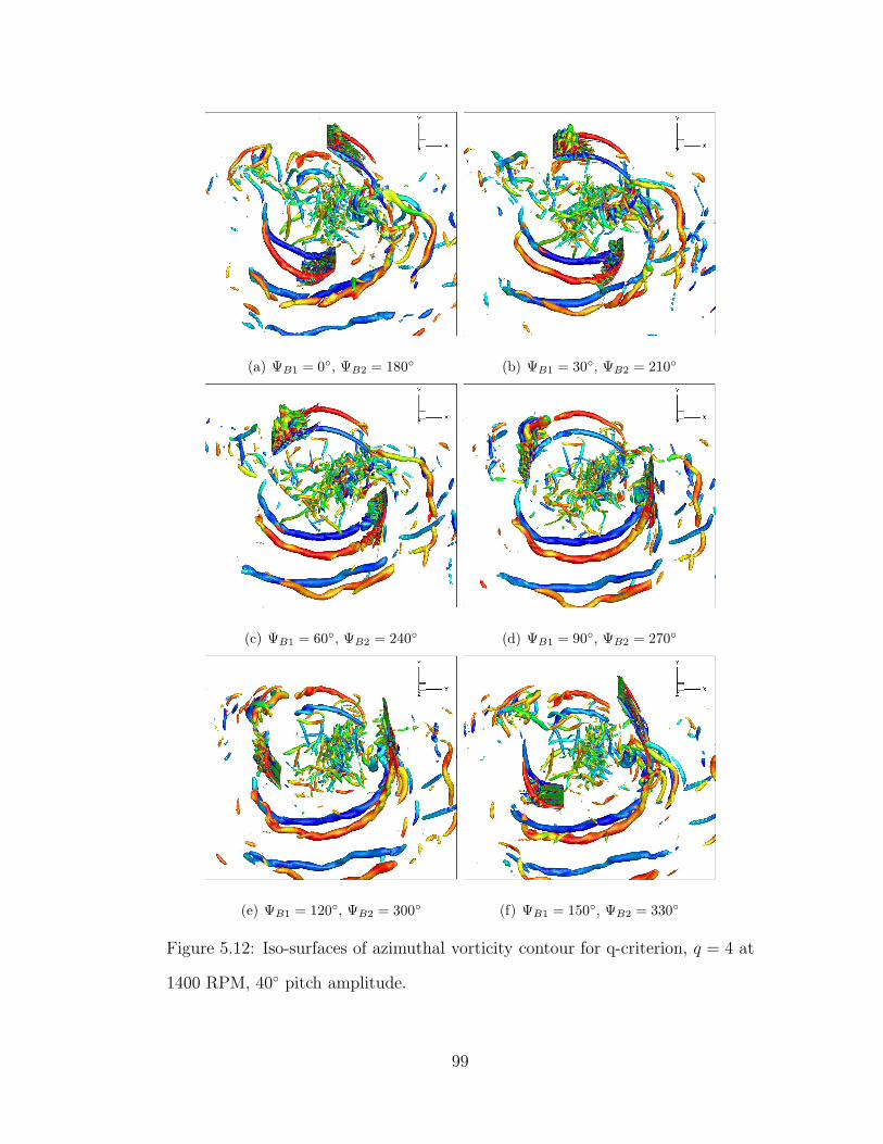
(a) ΨB1 = 0◦, ΨB2 = 180◦ (b) ΨB1 = 30◦, ΨB2 = 210◦

(c) ΨB1 = 60◦, ΨB2 = 240◦ (d) ΨB1 = 90◦, ΨB2 = 270◦

(e) ΨB1 = 120◦, ΨB2 = 300◦ (f) ΨB1 = 150◦, ΨB2 = 330◦

Figure 5.12: Iso-surfaces of azimuthal vorticity contour for q-criterion, q = 4 at

1400 RPM, 40◦ pitch amplitude.

99

(a) ΨB1 = 0◦, ΨB2 = 180◦ (b) ΨB1 = 30◦, ΨB2 = 210◦

(c) ΨB1 = 60◦, ΨB2 = 240◦ (d) ΨB1 = 90◦, ΨB2 = 270◦

(e) ΨB1 = 120◦, ΨB2 = 300◦ (f) ΨB1 = 150◦, ΨB2 = 330◦

Figure 5.13: Contours of spanwise vorticity at 1400 RPM, 40◦ pitch amplitude.

100

RMS values signifying a large amount of fluctuation from the mean value.

• Variations of vertical force and aerodynamic power over each blade show

that the virtual camber effect plays a large role in the performance of the

cyclocopter, and causes a degradation in performance for the blade at the

“top” of the cyclocopter cage, in comparison to the “bottom” blade. The

sidewise force variation indicated that its mean value was highly sensitive

to changes in blade pitch or deformation. Since small deviations in pitch

or deformation predictions can result in changes to the time history, thus

leading to large changes in the mean value. Therefore, performance in the

sidewise direction is very difficult to predict with CFD.

• Since the blades were fairly rigid and the RPM used in the experiments was

relatively low, the solution obtained from prescribing blade deformations

matched closely to the solution with no deformations. Thus, for this case,

it is largely unnecessary to include blade deflections.

• The cambered airfoil analysis showed that for the case tested, cambered

airfoils tended to negate the virtual camber effect but caused an overall

degradation in performance. However, additional work needs to be done

to ascertain the full benefit or detriment of using cambered blades.

• The spanwise thrust distribution was highly three-dimensional, and is re-

sultant from three different flow phenomena: the tip vortex, unsteady shed-

ding from the mid-span, and inflow velocities due to wake contraction. As

expected, it was found that inflow velocities acting downward decrease the

thrust, and velocities acting upward increase the thrust.

• The time-averaged inflow surface plots showed a large inflow through the

101

center of the rotor cage, with a region of reversed flow (upward) near

Ψ = 90◦. The iso-surfaces of q-criterion plots exhibited the extreme amount

of unsteadiness within the cyclocopter cage and the highly complex flow

structure; the contours of spanwise vorticity captured the wake contraction.

From the above results, it is seen that with CFD, significant insight into the

flow physics can be obtained in ways difficult to replicate in the laboratory.

102

Chapter 6

Conclusions

Within the last decade, interest in Rotary Wing Micro Air Vehicles (MAVs) has

grown due to their extreme versatility for a number of different mission scenarios.

However, the poor performance of conventional rotor designs at low Reynolds

numbers have allowed a flood of new, unconventional rotor designs to be tested

for MAVs. The rotor configuration described in this work was the cycloidal rotor,

essentially a “horizontal axis rotary wing” wherein the blades pitch and revolve

parallel to the rotational axis.

Previous experimental studies on the cycloidal rotor had mostly been under-

taken in the early 20th century, but problems with characterizing the complex

aerodynamics coupled with control issues due to the large centrifugal force from

rotor revolution forced the abandonment of the idea before it could be imple-

mented on aircraft. Recent studies of the cycloidal rotor have been focused on

the MAV-scale, since this rotor configuration allows for instantaneous thrust

vectoring plus extreme maneuverability. However, thus far only simple analyti-

cal models and preliminary, low-resolution CFD simulations have been used to

characterize the performance of the cycloidal rotor.

This current work sought to form a computational methodology by which

103

the performance of the cyclocopter could be predicted to reasonable accuracy.

Also, it focused on conducting unprecedented flowfield visualizations for the

cyclocopter to understand the complex aerodynamics in ways unachievable by

experiment. The following sections provide a brief summary of the contributions

made in this work, list specific observations obtained from the CFD analysis, and

suggest future research to further understanding of this unique rotor configura-

tion.

6.1 Summary

The objective of this work was to develop a high-fidelity, high-resolution com-

putational methodology to study the performance of the cyclocopter as well as

provide unprecedented insight into the flowfield. To accomplish this, an existing

compressible Reynolds-Average Navier-Stokes (RANS) Solver, OVERTURNS,

was modified to simulate the flight regime and blade motion of the cyclocopter.

The solver was first tested against a series of simple problems for verification

and validation before being applied to the cycloidal rotor. From the test cases,

the solver showed that it was adept at predicting the performance for both a

symmetric airfoil in steady, freestream conditions, and an unsteady, pitching

airfoil undergoing dynamic stall at high angles of attack. Dynamic stall flow

features were well captured as compared to 2-D VAWT experimental PIV mea-

surements. With confidence gained in the accuracy of the solver, the cycloidal

rotor could be simulated.

The cyclocopter experiments of Benedict et al. were chosen as a validation

case for numerical simulations of the cycloidal rotor. The hovering cyclocopter

rotor simulations were performed on structured body-fitted C-O blade mesh

104

overset onto a structured cylindrical background mesh. To compare performance,

both an RPM sweep with a fixed blade pitch amplitude and a collective pitch

sweep with a fixed RPM were tested. In addition to quantitative performance

comparisons to experimental results, a qualitative comparison was also made

between the PIV flow visualization and CFD results. In addition, cambered

blades were tested to negate the virtual camber effect, and preliminary results

were obtained for this design decision.

With validation of the flow solver accomplished, the flow physics were studied

with CFD predictions to characterize unsteady phenomena and understand the

three-dimensionality of the flowfield. The spanwise distribution of thrust was

investigated as a function of azimuthal angle, and the relationship between in-

flow and spanwise distribution was closely examined. Furthermore, the extreme

unsteadiness of the flowfield was visualized with the iso-surfaces of q-criterion

and vorticity contours, after which observations were made.

6.2 Specific Observations

Detailed conclusions drawn from the CFD analysis on the cycloidal rotor are

enumerated below.

1. Both the 2-D and 3-D solver were generally adept at obtaining vertical

forces comparable to experiment, while not capturing the sidewise force

well and underpredicting the power by a tare factor.

2. The total variation of thrust and power over time is easily obtained from

CFD but extremely difficult to achieve with experiments. The time histo-

ries of all the integrated values were periodic with large variations. Com-

105

paring one blade at different revolutions, or both blades shifted 180◦ rela-

tive to each other, the histories look very similar.

3. The sidewise force time history is particularly sensitive to changes in pitch

or deformation because the RMS value is much greater than the mean

value. Therefore an accurate mean value comparable to experiment is

difficult to predict with CFD.

4. The maximum vertical force and aerodynamic power for the cycloidal rotor

design is attained when the blade is at Ψ = 0◦, the lowest azimuthal

position. This is due to the virtual camber effect from blade rotation

which effectively imposes a positive camber on the symmetric airfoil at

the bottom of the cyclocopter cage, and a negative camber at the top.

However, testing of a 4.5% camber geometric configuration to counteract

virtual camber was not as effective as assumed: although the mean sidewise

force had reduced greatly, moderate decreases were observed for the thrusts

and powers produced.

5. The velocity vector plots between 3-D CFD and experimental DPIV show

a high level of accuracy in flow visualization for the CFD model. Almost

all of the flow structures captured in the time-averaged vector plots were

confirmed with other flowfield visualization methods.

6. The sidewise and vertical forces produced over the span show that the

spanwise forces are highly three-dimensional, and cannot be captured by

2-D CFD. Three main types of spanwise variation are observed: the effect

of tip vortex near the ends of the blade which cause local peaking of the

thrusts before dropping to zero at the tip; fluctuations due to unsteady

106

shedding from the blade at certain azimuthal locations; and different inflow

velocities seen by the mid and outboard spanwise sections due to wake

contraction.

7. The surface plots of time-averaged inflow as well as slices in the z-direction

corresponding to y-axis heights of various azimuthal locations clearly show

the skewing of the inflow as well as wake contraction through the rotor cage,

both phenomena observed through velocity vectors and vorticity contours.

A region of upwash was observed that was consistent with experiment.

8. The iso-surfaces of q-criterion from the 3-D results show a massive amount

of unsteadiness within the cyclocopter cage and larger tip vortices gen-

erated for the bottom blade than the top blade. The vorticity contours

clearly show the wake contraction from the top and bottom rotors as well

as skewing in the −z direction past the lower blade, previously observed in

the time-averaged spanwise velocity vectors. The strength of the tip vortex

shed by the bottom blade is larger due to the higher thrust produced at

this azimuthal location.

6.3 Future Work

Though the current CFD solver reasonably predicted performance and character-

ized the flowfield for the cycloidal rotor, there still remains a significant amount

of work to be undertaken for gaining further insight into the cycloidal rotor.

• The discrepancies in power and sidewise force remain to be resolved. These

discrepancies between CFD and experiment could possibly be reduced

through modeling of the support structures.

107

• A major potential for research is a two-way coupled CFD-CSD model of

the cyclocopter. The current study only initially prescribes grid deforma-

tions onto the blade mesh based on the steady blade periodic response

obtained from the structural dynamics code. In essence, the simulation

uses pre-deformed blades; a separate structural dynamics model is not be-

ing used to consider the deformations caused by the aerodynamic forces

during the simulation. Hence, the power required to deform the blades

is not accounted for in the numerical analysis. This may account for the

power discrepancy between CFD and experiment.

• Newer designs can be easily tested with CFD that would otherwise be diffi-

cult with experiment. Such new designs may include looking at asymmetric

pitch variation, camber, pitch axis location etc. to improve performance

capability.

• Though the effect of cambered airfoils was studied, only preliminary results

stemming from one test case were obtained. An RPM and collective sweep,

followed by investigation into the flow physics, is truly required to ascertain

if there is any benefit to be obtained from this blade design.

• The aerodynamics of the cyclocopter were only studied for hover in this

work. Studies of this rotor in forward flight or maneuvers have yet to be

conducted.

• An extension to the current work is the application of the cycloidal rotor to

extract power in a “cycloidal wind turbine” configuration. By forcing the

cycloidal rotor to act as if it were effectively in axial descent, the drag power

that can be obtained from the wind may be greater than a conventional

108

vertical axis wind turbine. However, preliminary tests by the author of this

work showed a significant dearth in the performance capability of the flow

solver to characterize cycloidal wind turbine performance trends, especially

at high tip speed ratios. Large-scale modifications to the code, possibly

with the implementation of a transition model, need to be undertaken

to correctly capture the flow physics of the cycloidal wind turbine. This

remains an area with significant potential for investigation.

Furthermore, future experiments can be conducted to additionally validate

the accuracy of the CFD prediction. Of these, paramount importance should

be given to a validation for the unsteady fluctuations of vertical and sidewise

force and power over time. Since only the integrated values of force and power

were compared between CFD and experiment, it is not known how well the CFD

solver performs at specific instances of the cyclocopter rotation. This validation

would be particularly important for the sidewise force which, as was discussed

earlier, had a mean predicted value which was particularly sensitive to changes

in blade pitch or deformation. Therefore, while discrepancies between CFD and

experiment may have been small for instantaneous values, these discrepancies

could build up over one rotor revolution to cause a large difference between

the mean value between CFD and experiment. An unsteady force and power

measurement would allow much better understanding of the solver’s performance

as compared with experiment, as well as suggest at which instantaneous values

of azimuth the solver prediction needs to improve. However, this requires a very

high sampling rate for the experiment, which may be difficult to achieve.

109

Appendix A

Numerical Work on Cycloidal Wind

Turbines

The first half of this appendix is to provide a comprehensive literature survey

of the numerical work on vertical axis and cycloidal wind turbines. Background

information on state-of-the-art simple analytical models and CFD analyses are

described here, with the the express purpose that future work on this topic may

be facilitated.

The latter half of this appendix is to present CFD validations with experiment

performed within the scope of the current work.

A.1 Numerical Work in Literature on VAWT

and CWT

A.1.1 Simple Analytical Models

Simplified numerical models of the VAWT have been developed by Paraschivoiu

and Allet [51] and Mertens et al. [52]. Paraschivoiu and Allet used incidence delay

110

methods to obtain aerodynamic performance predictions of dynamic stall on

Darrieus Wind Turbines and found that they correlate well the experimental data

of Sheldahl for a 17-m Sandia Wind Turbine. Mertens et al. used a combination

of axial momentum and blade element theory for an actuator plate representation

of the rotor to develop a multiple stream-tube model of skewed flow over a roof-

mounted H-Darrieus rotor. In addition, Reddy [53] used a multiple streamtube

model with the standard blade element theory applied to each of the streamtubes

to calculate the induced flow velocity on a Darrieus Wind Turbine. In turn,

this was used to estimate the force on each of the rotor blade elements. He

additionally explored the effects of changing geometrical parameters such as

blade solidity and rotor height-to-diameter ratios, as well as studied the transient

behavior of the rotor for a step change in wind speed or torque output.

A.1.2 CFD Simulations

Early CFD work on the VAWT was performed by Rajagopalan and Fanucci [54],

who used control volumes in cylindrical coordinates to map the computational

domain and modeled the turbine blades using a 2-D porous cylindrical shell; a

finite difference procedure was employed to solve the conservation of mass and

momentum equations. Allet et al. [55] numerically investigated the 2-D un-

steady flow around a NACA 0015 airfoil undergoing Darrieus rotational motion

using an incompressible Navier-Stokes solver with a Streamline Upwind Petrov-

Galerkin finite element method for discretization of the spatial terms. Ferreira

et al. [48] simulated dynamic stall on the blades of a 2-D straight-bladed H-

Darrieus VAWT and achieved validation of the results through comparison with

experimental measurements of blade loads and vorticity. Takahashi et al. [10]

111

used Direct Numerical Simulation (DNS) to model their VAWT experimental

setup and found that the results showed somewhat reasonable correlation with

experiment, though had difficulty predicting the exact trend of power coefficient

vs. TSR. Horiuchi et al. [56] investigated the flowfield around a VAWT using

Detached-Eddy Simulation with STAR-CD and examined the velocity profiles at

different locations downstream of the rotor. Numerical analysis for the cycloidal

rotor has been limited to the work of Hwang et al. [57], who used the STAR-CD

compressible flow solver to assess the pitch and phase angles for optimum power

generation on the cycloidal wind turbine.

A.1.3 Other Numerical Studies

Optimization studies have been performed to find the ideal pitching motion

which maximizes power generation on each blade as it travels around the azimuth

of the VAWT configurations. Paraschivoiu et al. [58] equated forces obtained

from blade element theory with actuator disk theory to iteratively converge

upon coefficients for a sinusoidal equation which describes optimal pitch for a

prescribed wind condition. Staelens et al. [59] expounded upon this previous

work to realize a sinusoidal function of local blade angle of attack that improved

power output while being mechanically feasible to implement.

A.2 Preliminary CFD Validation in the Cur-

rent Work

A CFD validation for the CWT was performed in the scope of the current work.

The TURNS code was previously validated against the VAWT PIV results and

112

force coefficients obtained by Ferreira et al. [8], as shown earlier in section 3.3.

For the CWT, the results of Hwang et al. [57] were used to examine the predictive

capabilities for unsteady time force history, as will be discussed in detail below.

A.2.1 Cycloidal Wind Turbine Validation

Due to the scarcity of experimental results in literature for a CWT, the nu-

merical results of Hwang et al. were used to verify the predictive accuracy of

OVERTURNS. However, these do not have experimental validation. The pitch-

ing motion of Hwang’s CWT is expressed through a pure sinusoidal variation

represented by the equation:

θ = θmax sin (Ψ − φe) (A.1)

where φe represents the angle of eccentricity of the offset (i.e. phase angle),

θmax indicates the pitch amplitude, and Ψ denotes the position of the blade

around the azimuth, equal to the product of the total time elapsed and the

rotational rate. The CWT setup is extremely similar to the schematic of the

cycloidal rotor shown in Figure 1.1.

Hwang et al. conducted numerical experiments for a four-bladed cycloidal

wind turbine using a symmetric NACA 0018 airfoil with a 0.45 m chord, a

rotational-radius-to-chord ratio of 3.56 and a span -to-chord ratio of 4.44. MSC/

PATRAN Command Language (a general purpose software for 3D geometry cre-

ation and grid generation) was used to generate a structured 8-node hexahedral

mesh. STAR-CD was employed with a k − ε high Reynolds turbulence model

to run this case. The optimum scenario for power generation as determined by

Hwang et al. was at a freestream wind speed of 13 m/s and a blade-tip speed

113

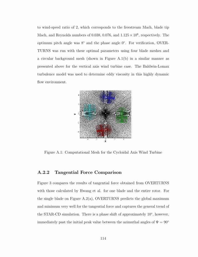
to wind-speed ratio of 2, which corresponds to the freestream Mach, blade tip

Mach, and Reynolds numbers of 0.038, 0.076, and 1.125×106, respectively. The

optimum pitch angle was 8◦ and the phase angle 0◦. For verification, OVER-

TURNS was run with these optimal parameters using four blade meshes and

a circular background mesh (shown in Figure A.1(b) in a similar manner as

presented above for the vertical axis wind turbine case. The Baldwin-Lomax

turbulence model was used to determine eddy viscosity in this highly dynamic

flow environment.

Figure A.1: Computational Mesh for the Cycloidal Axis Wind Turbine

A.2.2 Tangential Force Comparison

Figure 3 compares the results of tangential force obtained from OVERTURNS

with those calculated by Hwang et al. for one blade and the entire rotor. For

the single blade on Figure A.2(a), OVERTURNS predicts the global maximum

and minimum very well for the tangential force and captures the general trend of

the STAR-CD simulation. There is a phase shift of approximately 10◦, however,

immediately past the initial peak value between the azimuthal angles of Ψ = 90◦

114

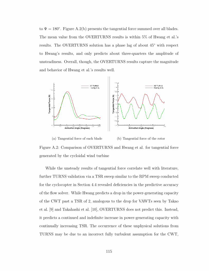
to Ψ = 180◦. Figure A.2(b) presents the tangential force summed over all blades.

The mean value from the OVERTURNS results is within 5% of Hwang et al.’s

results. The OVERTURNS solution has a phase lag of about 45◦ with respect

to Hwang’s results, and only predicts about three-quarters the amplitude of

unsteadiness. Overall, though, the OVERTURNS results capture the magnitude

and behavior of Hwang et al.’s results well.

(a) Tangential force of each blade (b) Tangential force of the rotor

Figure A.2: Comparison of OVERTURNS and Hwang et al. for tangential force

generated by the cycloidal wind turbine

While the unsteady results of tangential force correlate well with literature,

further TURNS validation via a TSR sweep similar to the RPM sweep conducted

for the cyclocopter in Section 4.4 revealed deficiencies in the predictive accuracy

of the flow solver. While Hwang predicts a drop in the power-generating capacity

of the CWT past a TSR of 2, analogous to the drop for VAWTs seen by Takao

et al. [9] and Takahashi et al. [10], OVERTURNS does not predict this. Instead,

it predicts a continued and indefinite increase in power-generating capacity with

continually increasing TSR. The occurrence of these unphysical solutions from

TURNS may be due to an incorrect fully turbulent assumption for the CWT,

115

or due to TURNS’ inability to capture separated flow. Further investigation is

needed into this issue, possibly with the future implementation of a transition

model into TURNS.

A.2.3 Summary

In this appendix, it was seen that experimental as well as numerical investigation

into the performance of VAWTs and CWTs is still relatively limited. Though cer-

tain preliminary studies have been performed to predict the aerodynamic forces

on VAWTs, there have been no comprehensive insights into the flow physics of

the VAWT or CWT in literature. Preliminary CFD studies by the current work

into the performance of the CWT show that while TURNS can qualitatively

visualize the flowfield well and capture the unsteady aerodynamics for low tip

speed ratios, the CFD predictions become unphysical with higher TSRs. Much

future work remains for modifying the flow solver to generate accurate predic-

tions of the VAWT flowfield, and VAWTs and CWTs continue to be a largely

unexplored area of potential research.

116

Appendix B

CFD Simulation of an Unsteady

Pitching Airfoil at Low Reynolds

Numbers

Unsteady lift, drag, and moment coefficient results were obtained for the NACA

0010 airfoil for pitching amplitudes of 0-30 with respect to freestream conditions

of Re = 30, 000 and M∞ = 0.047 at increments of 5◦, as consistent with the

experimental setup of Benedict et al. However, these are merely CFD predic-

tions and do not have any experimental validation. The results for coefficient of

lift, drag, and moment at quarter-chord position for pitch amplitude of 30◦ are

presented in Figure B.1.

From the plots, distinct changes in the flow can be noted through their effect

on lift, drag, and moment, and through examination of the pressure contours

over the airfoil. As the airfoil pitches up from zero degrees, there is a somewhat

steady rise of Cl, Cd, and a small drop followed by a region of constant Cm

from 0 − 23◦ due to the formation of low pressure suction peak at the leading

edge on the upper surface and a high pressure stagnation region on the lower

117

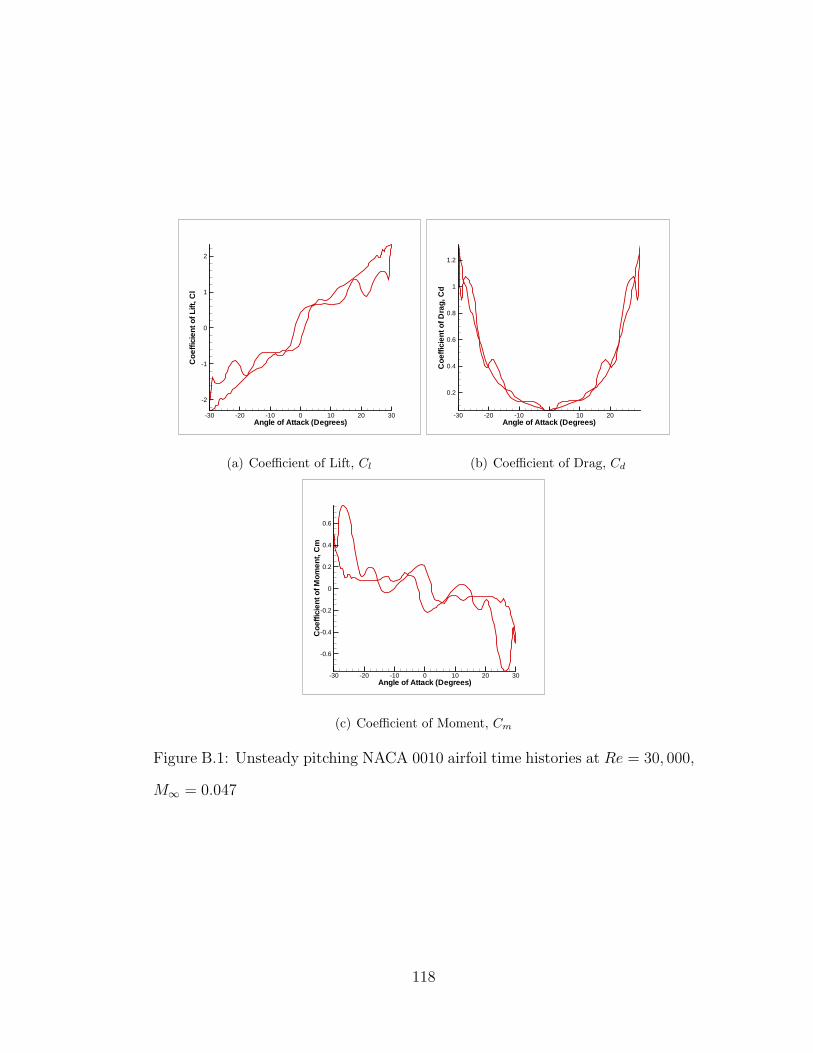
Angle of Attack (Degrees)

Coe

ffici

ento

fLift

,Cl

-30 -20 -10 0 10 20 30

-2

-1

0

1

2

(a) Coefficient of Lift, Cl

Angle of Attack (Degrees)

Coe

ffici

ento

fDra

g,C

d

-30 -20 -10 0 10 20

0.2

0.4

0.6

0.8

1

1.2

(b) Coefficient of Drag, Cd

Angle of Attack (Degrees)

Coe

ffici

ento

fMom

ent,

Cm

-30 -20 -10 0 10 20 30

-0.6

-0.4

-0.2

0

0.2

0.4

0.6

(c) Coefficient of Moment, Cm

Figure B.1: Unsteady pitching NACA 0010 airfoil time histories at Re = 30, 000,

M∞ = 0.047

118

surface. As the airfoil pitches from 23 − 30◦, the rollup and detachment of the

leading edge vortex leads to oscillations in Cl, large increases in Cd and steady

decrease of Cm nose-down. From 30 − 27◦ pitching down, a large vortex is shed

from the upper surface at around 3/4-chord. There is also the formation of a

small, albeit strong vortex at the trailing edge of the airfoil, and the interaction

between these two vortices leads to a sharp drop in Cl, Cd, and Cm (nose-down

pitching moment). From 27− 4◦ pitching down, the intensification of the vortex

formed on the trailing edge at 27◦, and the large region of low pressure formed by

the shedding of this vortex which extends from 3/4-chord position downstream,

leads to decrease in Cl and Cd with large oscillations, and a nose-up Cm. From

−4◦ to 4◦ pitch down, the shedding of this low pressure region and its interaction

with other small vortices that form on the trailing edge leads to a drop in Cl,

somewhat constant Cd and another nose-up pitching moment. The rest of the

lower pitching cycle from −4◦ to −30◦ back to 0◦ is a repetition of the upper

pitching cycle on the lower surface.

119

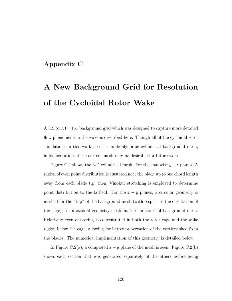
Appendix C

A New Background Grid for Resolution

of the Cycloidal Rotor Wake

A 321×151×151 background grid which was designed to capture more detailed

flow phenomena in the wake is described here. Though all of the cycloidal rotor

simulations in this work used a simple algebraic cylindrical background mesh,

implementation of the current mesh may be desirable for future work.

Figure C.1 shows the 3-D cylindrical mesh. For the spanwise y− z planes, A

region of even point distribution is clustered near the blade up to one chord length

away from each blade tip; then, Vinokur stretching is employed to determine

point distribution to the farfield. For the x − y planes, a circular geometry is

meshed for the “top” of the background mesh (with respect to the orientation of

the cage); a trapezoidal geometry exists at the “bottom” of background mesh.

Relatively even clustering is concentrated in both the rotor cage and the wake

region below the cage, allowing for better preservation of the vortices shed from

the blades. The numerical implementation of this geometry is detailed below.

In Figure C.2(a), a completed x− y plane of the mesh is seen. Figure C.2(b)

shows each section that was generated separately of the others before being

120

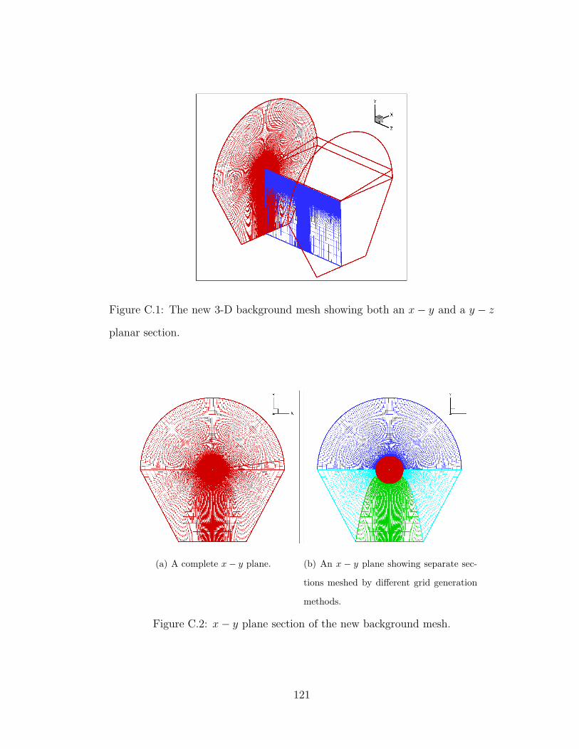
Figure C.1: The new 3-D background mesh showing both an x − y and a y − z

planar section.

(a) A complete x − y plane. (b) An x − y plane showing separate sec-

tions meshed by different grid generation

methods.

Figure C.2: x − y plane section of the new background mesh.

121

integrated into the framework of the entire mesh geometry. In this figure, the

“center” rotor cage region (in red) was generated completely using an algebraic

distribution with constant spacing in both the tangential and radial directions,

such that all the flow features near the rotor cage could be captured to a high

resolution and accuracy. The upper cylindrical region (in blue) was generated

using even algebraic spacing in the spanwise direction and Vinokur stretching

in the radial direction. For the lower trapezoidal distribution, the parabolic

boundary between the lower side regions (in cyan) and the lower center region

(in green) was determined using a least squares fit through a number of points

as prescribed by the user. Thus, the lower center region is variable in size and

can be enlarged or compressed based on the cycloidal rotor case of interest. The

points along the radial direction of the parabolic line, as well as the clustering at

the bottom of the lower center region, were distributed using Vinokur stretching.

For all the mesh points within the lower side regions and the lower center region,

a crude algebraic distribution was first generated. Then, Poisson-based elliptic

grid generation method was used to provide a smooth distribution for the interior

nodal points, given the boundary point distribution. More information on elliptic

grid generation can be found in Thompson [26].

122

Bibliography

[1] Sachse, H., “Kirsten-Boeing Propeller,” Technical Memorandum no. 351,

NACA, 1926.

[2] Strandgren, C. B., “The Theory of the Strandgren Cyclogiro,” Technical

Memorandum no. 727, NACA, 1933.

[3] Wheatley, J. B., “Simplified Analysis of the Cyclogyro Rotating Wing Sys-

tem,” Report no. 467, NACA, 1933.

[4] Wheatley, J. B. and Windler, R., “Wind Tunnel Tests of a Cyclogiro Rotor,”

Technical Note no. 528, NACA, 1935.

[5] Darrieus, G. J. M., “Turbine Having its Rotating Shaft Transverse to the

Flow of the Current,” U.S. Patent no. 1,835,018 , 1931.

[6] Sheldahl, R. E., “Comparison of Field and Wind Tunnel Darrieus Wind Tur-

bine Data,” Report SAND80-2469, Sandia National Laboratories, Aerother-

modynamics Division, Sandia National Laboratories, Albuquerque, New

Mexico, 1981.

[7] Sheldahl, R. E. and Klimas, P. C., “Aerodynamic Characteristics of Seven

Symmetrical Airfoil Sections Through 180-Degree Angle of Attack for Use in

123

Aerodynamic Analysis of Vertical Axis Wind Turbines,” Report SAND80-

2114, Sandia National Laboratories, Albuquerque, New Mexico, 1981.

[8] Ferreira, C. S., van Bussel, G., and van Kuik, G., “2D PIV Visualization

of Dynamic Stall on a Vertical Axis Wind Turbine,” 45th AIAA Aerospace

Sciences Meeting and Exhibit , No. AIAA 2007-1366, Reno, NV, Jul. 2007.

[9] Takao, M. et al., “Experimental Study of a Straight-Bladed Vertical Axis

Wind Turbine with a Directed Guide Vane Row,” Proceedings of the 28th

International Conference on Ocean, Offshore, and Arctic Engineering , Hon-

olulu, HI, Jun. 2009.

[10] Takahashi, S., Ohya, Y., Takashi, K., and Watanabe, K., “Numerical and

Experimental Studies of Airfoils Suitable for Vertical Axis Wind Turbines

and an Application of Wind-Energy Collecting Structure for Higher Per-

formance,” The Fourth International Symposium on Computational Wind

Engineering (CWE 2006), Yokohama, Japan, 2006, pp. 327–330.

[11] Kiwata, T. et al., “Performance of a Vertical Axis Wind Turbine with

Variable-Pitch Straight Blades using a Linkage Mechanism,” Journal of En-

vironment and Engineering , Vol. 5, No. 1, 2010, pp. 213–225.

[12] Hwang, I. et al., “Experimental Investigation of VTOL UAV Cyclocopter

with Four Rotors,” 48th AIAA/ASME/ASCE/AHS/ASC Structures, Struc-

tural Dynamics, and Material Conference, No. AIAA 2007-2247, Honolulu,

HI, Apr. 23–26 2007.

124

[13] Yu, H., Bin, L. K., and Rong, H. W., “The Research on the Performance

of Cyclogiro,” 6th AIAA Aviation Technology, Integration, and Operations

Conference, No. AIAA 2006-7704, Wichita, KS, Sep. 25–27 2006.

[14] Benedict, M., Ramasamy, M., Chopra, I., and Leishman, J. G., “Exper-

iments on the Optimization of MAV-Scale Cycloidal Rotor Characteris-

tics towards Improving their Aerodynamic Performance,” American He-

licopter Society International Specialists Meeting on Unmanned Rotorcraft ,

Phoenix, AZ, Jan. 20–22 2009.

[15] Benedict, M., Jarugumilli, T., and Chopra, I., “Design and Development

of a Hover-Capable Cyclocopter Micro Air Vehicle,” American Helicopter

Society 65th Annual Forum, Grapevine, TX, May 27–29 2009.

[16] Benedict, M., Jarugumilli, T., and Chopra, I., “Experimental Performance

Optimization of a MAV-Scale Cycloidal Rotor,” Proceedings of the AHS

Specialists’ Meeting on Aeromechanics, San Francisco, CA, Jan 20–22 2010.

[17] Yun, C. Y. et al., “A New VTOL UAV Cyclocopter with Cycloidal Blades

System,” American Helicopter Society 60th Annual Forum, Baltimore, MD,

June 7–10 2004.

[18] McNabb, M. L., Development of a Cycloidal Propulsion Computer Model

and Comparison with Experiment , Masters Thesis, Mississippi State Uni-

versity, Department of Aerospace Engineering, December 2001.

[19] Garrick, I. E., “Propulsion of a Flapping and Oscillating Airfoil,” Report

no. 567, NACA, 1937.

125

[20] Parsons, E., Investigation and Characterization of a Cycloidal Rotor for

Application to a Micro-Air Vehicle, Masters Thesis, University of Maryland,

Department of Aerospace Engineering, 2005.

[21] Benedict, M., Mattaboni, M., Chopra, I., and Masarati, P., “Aeroelas-

tic Analysis of a MAV-Scale Cycloidal Rotor,” Proceedings of the 51st

AIAA/ASME/ASCE/AHS/ASC Structures, Structural Dynamics, and Ma-

terials Conference, Orlando, FL, Apr. 12–15 2010.

[22] Iosilevskii, G. and Levy, Y., “Experimental and Numerical Study of Cyclo-

giro Aerodynamics,” AIAA Journal , Vol. 44, No. 12, 2006, pp. 2866–2870.

[23] Lakshminarayan, V. K. and Baeder, J. D., “High Resolution Computational

Investigation of Trimmed Coaxial Rotor Aerodynamics in Hover,” Journal

of the American Helicopter Society , Vol. 54, No. 4, 2009, pp. 042008–1 –

042008–21.

[24] Lakshminarayan, V. K., Computational Investigation of Micro-Scale Coaxial

Rotor Aerodynamics in Hover , Ph.D. Dissertation, University of Maryland,

Department of Aerospace Engineering, 2009.

[25] Vinokur, M., “On One-Dimensional Stretching Functions for Finite Dif-

ference Calculations,” Journal of Computational Physics , Vol. 50, 1983,

pp. 215–234.

[26] Thompson, J. F., Soni, B. K., and Weatherill, N. P., Handbook of Grid

Generation, CRC Press, 1999.

126

[27] Thompson, J. F., Aspects of Numerical Grid Generation - Current Science

and Art , Masters Thesis, Mississippi State University, NSF Engineering

Research Center for Computational Field Simulation, 1993.

[28] Alsalihi, Z., “Two-Dimensional Hyperbolic Grid Generation,” Technical

Note 162, von Karman Institute for Fluid Dynamics, 1987.

[29] Cordova, J. Q. and Barth, T. J., “Grid Generation for General 2-D Re-

gions Using Hyperbolic Equations,” 26th AIAA Aerospace Sciences Meet-

ing , Reno, NV, Jan. 1988.

[30] Kinsey, D. W. and Barth, T. J., “Description of a Hyperbolic Grid Gener-

ating Procedure for Arbitrary Two-Dimensional Bodies,” Technical Memo-

randum TM-84-191, Flight Dynamics Laboratory, Air Force Wright Aero-

nautical Laboratories, Wright-Patterson Air Force Base, 1984.

[31] Chan, W. M. and Steger, J. L., “A Generalized Scheme for Three-

Dimensional Hyperbolic Grid Generation,” AIAA Paper 91-1588-CP , 1991.

[32] Lee, Y., On Overset Grid Connectivity and Automated Vortex Tracking

in Rotorcraft , Ph.D. Dissertation, University of Maryland, Department of

Aerospace Engineering, 2008.

[33] Sitaraman, J., CFD Based Unsteady Aerodynamic Modeling for Rotor

Aeroelastic Analysis, Ph.D. Dissertation, University of Maryland, Depart-

ment of Aerospace Engineering, 2003.

[34] Hodges, D. H. and Dowell, E. H., “Nonlinear Equations of Motion for the

Elastic Bending and Torsion of Twisted Nonuniform Rotor Blades,” Tech-

nical Note D-7818, NASA, 1974.

127

[35] White, F. M., Viscous Fluid Flow , McGraw-Hill, Inc., New York, NY, 1991.

[36] Baldwin, B. S. and Lomax, H., “Thin Layer Approximation and Algebraic

Model for Separated Turbulent Flows,” AIAA Paper 78-257 , 1978.

[37] Spalart, P. R. and Allmaras, S. R., “A One-equation Turbulence Model for

Aerodynamic Flows,” 30th AIAA Aerospace Sciences Meeting and Exhibit ,

No. AIAA 1992-0439, Reno, NV, Jan. 1992.

[38] van Leer, B., “Towards the Ultimate Conservative Difference Scheme,”

Journal of Computational Physics , Vol. 32, No. 1, 1979, pp. 101–136.

[39] Roe, P. L., “Approximate Riemann Solvers, Parameter Vectors and Differ-

ence Schemes,” Journal of Computational Physics , Vol. 135, No. 2, 1997,

pp. 250–258.

[40] Turkel, E., “Preconditioning Techniques in Computational Fluid Dynam-

ics,” Annual Review of Fluid Mechanics , Vol. 31, 1999, pp. 385–416.

[41] Jameson, A., “Time Dependent Calculations Using Multigrid, with Appli-

cations to Unsteady Flows Past Airfoils and Wings,” AIAA Paper 91-1596 ,

1991.

[42] Hirsch, C., Numerical Computation of Internal and External Flows, Vol. 2 ,

Wiley Publishers, 1990.

[43] Pulliam, T. H. and Chaussee, D. S., “A Diagonal Form of an Implicit

Approximate Factorization Algorithm,” Journal of Computational Physics ,

Vol. 39, No. 2, Feb. 1981, pp. 347–363.

128

[44] Lutz, T., Wurz, W., and Wagner, S., “Numerical Optimization and Wind-

Tunnel Testing of Low Reynolds Number Airfoils,” Fixed and Flapping Wing

Aerodynamics for Micro Air Vehcile Applications, edited by T. J. Mueller,

AIAA, 2001, pp. 169–190.

[45] McAlister, K. W., Pucci, S. L., McCroskey, W. J., and Carr, L. W., “An Ex-

perimental Study of Dynamic Stall on Advanced Airfoil Sections, Pressure

and Force Data,” Technical Memorandum TM-84245, NASA, 1982.

[46] Tuncer, I. H., Wu, J. C., and Wang, C. M., “Theoretical and Numeri-

cal Studies of Oscillating Airfoils,” AIAA Journal , Vol. 28, No. 9, 1990,

pp. 1615 – 1624.

[47] Coene, R., “Elements of the Aerodynamic Theory of Cyclogyro Wing Sys-

tems with Concentrator Effects,” Technical Report LR-338, Delft University

of Technology - Aerospace Faculty, Delft, the Netherlands, Oct. 1983.

[48] Ferreira, C. S. et al., “2D CFD Simulation of Dynamic Stall on a Vertical

Axis Wind Turbine: Verification and Validation with PIV Measurements,”

45th AIAA Aerospace Sciences Meeting and Exhibit / ASME Wind Energy

Symposium, Reno, NV, Jan. 2007.

[49] Jeong, J. and Hussain, F., “On the Identification of a Vortex,” Journal of

Fluid Mechanics , Vol. 285, 1995, pp. 69–94.

[50] Leishman, J. G., Principles of Helicopter Aerodynamics, Cambridge Uni-

versity Press, New York, NY, 2006.

129

[51] Paraschivoiu, I. and Allet, A., “Aerodynamic Analysis of the Darrieus

Wind Turbines Including Dynamic Stall Effects,” Journal of Propulsion

and Power , Vol. 4, No. 5, 1988, pp. 472–477.

[52] Mertens, S. et al., “Performance of a High Tip Speed Ratio H-Darrieus in

the Skewed Flow on on a Roof,” 41st AIAA Aerospace Sciences Meeting

and Exhibit , No. AIAA 2003-0523, Reno, NV, Jan. 2003.

[53] Reddy, G. B., The Darrieus Wind Turbine: An Analytical Performance

Study , Masters Thesis, Texas Tech University, Department of Mechanical

Engineering, 1976.

[54] Rajagopalan, R. and Fanucci, J., “Finite Difference Model for Vertical Axis

Wind Turbines,” Journal of Propulsion and Power , Vol. 1, No. 6, 1985,

pp. 432–436.

[55] Allet, A. et al., “Numerical Simulation of Dynamic Stall Around an Airfoil

in Darrieus Motion,” Journal of Solar Energy Engineering , Vol. 121, Feb.

1999, pp. 69–76.

[56] Horiuchi, K., Ushiyama, I., and Kazuichi, S., “Straight Wing Vertical Axis

Wind Turbines: A Flow Analysis,” Wind Engineering , Vol. 29, No. 3, 2005,

pp. 243–252.

[57] Hwang, I. S. et al., “Efficiency Improvement of a Cycloidal Wind Turbine

by Active Control of Blade Motion,” Tech. rep., School of Mechanical and

Aerospace Engineering, Seoul National University, Seoul, Rep. of Korea,

2006.

130

[58] Paraschivoiu, I. et al., “H-Darrieus Wind Turbine with Blade Pitch Con-

trol,” International Journal of Rotating Machinery , Vol. 2009, Article ID

505343, 2009.

[59] Staelens, Y. et al., “A Straight-Bladed Variable-Pitch VAWT Concept for

Improved Power Generation,” 41st AIAA Aerospace Sciences Meeting and

Exhibit , No. AIAA 2003-0524, Reno, NV, 2003.

131