CAL P__AD-A244 033 -- __-

INVESTIGATION OF UNSTEADY FLOWIN AN ANNULAR CASCADE

1 October 1991

CONTRACT F49620-87-C-0053

Research sponsored by the Air Force Office of Scientific Research (AFSC),under contractF49620-87-C-0053. The United States Government is authorized to reproduce anddistribute reprints for governmental purposes notwithstanding any copyright notation

I hereon.

Prepared by:

Dr. William K. GeorgeDr. Dale B. Taulbee

I Dr. Richard L. LeBoeuf

State University of New York at BuffaloDept. of Mechanical and Aerospace Engineering

..... I -91-19199

CALSPAN UB RESEARCH CENTER P0 BOX 400. BUFFALO. NEW YORK 14225 TEL (716) 631 6900

Unclassified U NCLA Sol DSIECuRITY CLASS FiCAT ON OF TH)S PACGE

Form ApprovedREPORT DOCUMENTATION PAGE OMB No. 0704-01"

a. REPORT SECURITY CLASSIFICATION lb. RESTRICTIVE MARKINGS

Unclassified None2a. SECURITY CLASSIFICATION AUTHORITY 3. DISTRIBUTION /AVAILABILITY OF REPORT

N/A2b. DECLASSIFICATION/DOWNGRADING SCHEDULE Unlimited

N/AI 4. PERFORMING ORGANIZATION REPORT NUMBER(S) S. MONITORING ORGANIZATION REPORT NUMBER(S)

WA770

6a. NAME OF PERFORMING ORGANIZATION 6b. OFFICE SYMBOL 7a. NAME OF MONITORING ORGANIZATION

Calspan-UB Research Center (if applicable) AFOSRI/A _f;"--AAR(CUBRC) R , /. ol I ng AFA nC 20 I. -12 R

6c. ADDRESS (City, State, and ZIP Code) 7b. ADDRESS (City, State, and ZIP Code)PO Box 400 ,.i OSR/ IRABuffalo, NY 14225 Boling AF nP .2...A.

I 8a. NAME OF FUNDING/SPONSORING 8b OFFICE SYMBOL 9 PROCUREMENT INSTRUMENT IDENTIFICATION NUMBERORGANIZATION Air Force Office (if al /

of Scientific Research F49620-87-C-0053

9c, ADDRESS (City, State, and ZIP Code) 10 SOURCE OF FUNDING NUMBERS

Boln i oc aePROGRAM PROJECT TASK WORK UNITBaln°ArFrce BsWashington, DC 20332-6448 EN O3 O A

11 TITLE (include Security Classification)

"Investigation of Unsteady Flow in an Annular Cascade"

12. PERSONAL AUTHOR(S)Dr. William K. George; Dr. Dale B. Taulbee, Richard L. LeBoeuf

13a. TYPE OF REPORT 13b TIME COVERED 14. DATE OF REPORT (Year, Month Day) 15. PAGE COUNTFinal Technical FROM 7/87 TO _J_./.. 1 October 1991 107

16. SUPPLEMENTARY NOTATION

17. COSATI CODES 18 C TiuJ oryy kmFIELD GROUP SUB-GROUP , n,,, - ,. ,r -- ---

19. ABSTRACT (Continue on reverse if necessary and identify by block number)

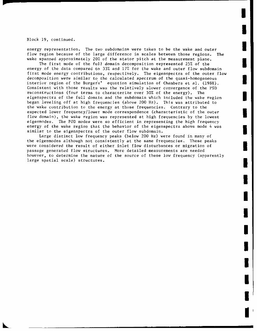
The proper orthogonal decomposition (POD)(Lumley 1967) was used to test the hypothesis

that there exist a set of functions which characterize a turbine stator exit flowfield andwhose dynamics may explain some of the complex behavior in downstream blade rows. Thedecomposition was applied to three component triple-wire probe measurements of a large-scale annular stator model exit flowfield. This study represents the first application ofthe orthogonal decomposition to directly measured three component data, and one of the first

applications to an applied engineering flow.The full three-component cross-spectral tensor was produced from simultaneous multi-

point triple-wire probe measurements. The measurements were taken across one stator pitch,

at the passage midspan, 107 axial chord downstream of the stator trailing edge. Theresulting 1089 cross-spectral estimates were then decomposed to obtain the eigenspectra and

eigenmodes of the midspan flowfield. In addition, the POD was applied to two subdomains

of the passage flowfield in order to increase the convergence rate of the (cont'd)

20 DISTRIBUTION/AVAILABILITY OF ABSTRACT 21 ABSTRACT SECURITY CLASSIFICATIONM) UNCLASSIFIED/UNLIMITED 0 SAME AS RPT 0 DTIC USERS3 22a NA OF 5SPONSIBLF INDlIVIDUAL 12bTLP10 .I-1-e Area C y) 1 22c OFFICE YMAAL

DD Form 1473, JUN 86 Previous editions are obsolete. SECURITY CLASSIFICAT N OF THIS PAGE

U NCLAbi bl -I "

I

IBlock 19, continued.

energy representation. The two subdomains were taken to be the wake and outer Iflow region because of the large difference in scales between those regions. Thewake spanned approximately 20% of the stator pitch at the measurement plane.

The first mode of the full domain decomposition represented 25% of the Ienergy of the data compared to 33% and 17% for the wake and outer flow subdomainfirst mode energy contributions, respectively. The eigenspectra of the outer flowdecomposition were similar to the calculated spectrum of the quasi-homogeneousinterior region of the Burgers' equation simulation of Chambers et al. (1988).Consistent with those results was the relatively slower convergence of the PSDreconstructions (four terms to characterize over 50% of the energy). Theeigenspectra of the full domain and the subdomain which included the wake region Ibegan leveling off at high frequencies (above 200 Hz). This was attributed tothe wake contribution to the energy at those frequencies. Contrary to theexpected lower frequency/lower mode correspondence (characteristic of the outerflow domain), the wake region was represented at high frequencies by the lowesteigenmodes. The POD modes were so efficient in representing the high frequencyenergy of the wake region that the behavior of the eigenspectra above mode 4 wassimilar to the eigenspectra of the outer flow subdomain. I

Large distinct low frequency peaks (below 200 Hz) were found in many ofthe eigenmodes although not consistently at the same frequencies. These peakswere considered the result of either inlet flow disturbances or migration ofpassage generated flow structures. More detailed measurements are neededhowever, to determine the nature of the source of these low frequency (apparentlylarge spatial scale) structures.

UIIIIIIII

I

TABLE OF CONTENTS

U Project Personnel ................................................................................... i

I Introduction ...................................................................................... 1

2 Proper Orthogonal Decomposition ................................................................. 6

2.1 Theory ........................................................................................................... 6

2.1.1 Stationary and Homogeneous Directions ............................................................. 8

2.1.2 T his A pplication ............................................................................................ 9

3 Spectral Analysis .................................................................................. 13

4 The Experiment .................................................................................... 1 5;

4.1 Experimental Facility .............................................................................................. 15

U 4.1.1 Wind Tunnel ....................................................................... 15

4.1.2 Probe Traverses ........................................................................................ 16

4 .2 In stru m entatio n ........................................................................................................... 17

4 .3 S am p ling C riteria ........................................................................................................ 2 1

4.4 Hot-Wire Implementation ......................................................................................... 23

4.4.1 Response Equations .................................................................................. 24

4.4.2 Parameter Optimization ............................................................................ 29

4.4.3 Calibration Procedure ................................................................................ 33

4.4.4 Triple-Wire Decoding ................................................................................ 36IPreliminary Measurements ....................................................................... 3

5.1 Inlet Flow fi eld ............................................................................................................ 38

5 .2 E xit Flow field ............................................................................................................ 40

5.2.1 .......................................................................................... . . . 40 .

5.2.2 Five-Hole Probe ..................................................................................... 40 J5.3 Airfoil Surface Static Pressure Distributions ................................................................ 47, :1

' . I

6 Results and Discussion.....................................................53

6.1 R eynolds Stresses ........................................................................................................ 53

6.2 Proper Orthogonal Decomposition .......................................................................... 55

6.2.1 Full Domain: 0-100% Pitch ....................................... 55

6.2.2 Subdomain Decomposition ...................................................................... 73I7 Conclusions and Recommendations ............................................................ 95

1 8 Publications ........................................................................................ 98

1 8.1 Directly Related to W ork ....................................................................................... 98

8.2 Other Papers Published by Principals Bearing SomeRelation to W ork ........................................................................................................ 98

i A POD Formulation ................................................................................... 100

B ibliography ........................................................................................... 102

iIII

I1

Project Personnel

The following personnel contributed to the research described in this report:

Faculty:

William K. George, Project Director

Dale B. Taulbee, Co-Project Director

University Support Staff:

Scott Woodward, Laboratory Technician

Eileen Graber, Secretar,

Graduate Students:

Aamir Shabbir, Research Associate, (6-87 to 8-88)

Richard LcBoeuf. Research Assistant (6-87 to 8-90) - PhD received 9-91, Thesis Title "Applicationof the Proper Orthogonal Decomposition Techniques to an Annular Cascade Flowfield"

James Sonnenmeier, Research Assistant, (6-87 to 8-88) - PhD in progress, expected 9-92.

III

I

I Introduction

IThe flow and heat transfer that occur in a turbine represent one of the most complicated environ-

I ments seen in a practical machine. The flow is unsteady, transonic, three-dimensional, turbulent,

3 non-isothermal and subject to strong body forces. The principle factor that limits the efficiency of

gas turbine engines is the inability of turbine components to withstand high temperat ure. and large

heat transfer rates. Turbine performance is also limited by the aerodynamic losses of the working

fluid. Accordingly, attempts to understand, predict, and control these phenomena have pla~ed a

I central role in gas-turbine research.

3 Satisfactory turbine designs have been achieved due to the development of a sound understanding

of the flow and heat transfer mechanisms that define the mean-flow performance and to advances in

3 materials and manufacturing processes. Rising fuel costs and concerns about noise and combustion

emissions spurred a flurry of more detailed turbine research activities especially since the early

1980's. Current research activities have been dir- tari at moving beyond the mean-flow mechanics

into investigations of the time-dependent aspects of the flow. Some of these aspects lie in the realm

of deterministic unsteady fluid mechanics, while others belong to the subject of turbulence.

Examination of the flow through a stationary row of blades has been carried out for a number

of blade row geometries, both annular and linear, using a broad range of experimental techniques.

U These methods have included both qualitative and quantitative measures of the flow. Qualitative

measures have primarily consisted of flow visualization utilizing smoke in the mainstream and oils

and other substances on surfaces (summarized by Sieverding 1985). Quantitative measurements

have primarily consisted of five and three hole pressure probe measurements of static pressure,

total pressure, and mean velocity (examples include Dring et al. (1986), Moustapha et al. (1985),

U Gregory-Smith and Graves (1983), Moore and Adhye (1985), and Sieverding et al. (1984)). In

addition, hot-wire anemometry with single and multiple hot-wire and film probes (for example,

Sharma et al. 1985, Hodson 1985, Gregory-Smith and Graves 1983, Gorton and Lakshminarayana

*

I1976 and Raj and Lakshminarayana 1973) and laser-Doppler velocimetry (LDV) (Bailey 1979) have

3 been used to determine flow velocities and Reynolds stresses. The results of the former studies of

turbine passage flow have illucidated the non-uniformity and unsteadiness including the production

of passage and horseshoe vortices. The appearance of these flow structures results in high loss regions

3 in blade row exit flowfields as illustrated by total pressure loss contours (v. Dring et al. 1986).

To complement the studies of turbine aerodynamics, turbine heat transfer investigations have

been carried out by a number of researchers. One of the most important influences on the local

heat transfer to a turbine blade or vane is the time-unsteady condition of the flow as it enters the

blade row (Graham 1980). A categorization of the different contributions to the unsteadiness was

Sgiven by Evans (1975) as a separation of the random turbulence from the inherent periodicities of a

flowfield. The aggregate affects of such flow unsteadiness on heat transfer has been shown to have a

I significant effect on the heat transfer through experimental studies using thermocouple instrumented

airfoils (e.g. Graziani, et al. 1980 and Blair et al., 1989a,b). Higher resolution turbine rotor heat

transfer measurements (Dunn 1986, Dunn et al. 1986 and later Guenette et al. (1989) and Dunn,

3 et al. 1990) clearly demonstrate the importance of the random velocity components to the unsteady

heat transfer. It is expected that the flow seen by a given blade would contain the blade passing

I periodicities (along with its harmonics). However, strong heat transfer signals are seen acrosb a .wii'

frequency spectrum, both above and below that of blade passage.

Even in the absence of viscosity, the pressure fields generated by interactions between rotor and

I stator blade rows can be expected to produce time varying phenomena whose freqiency spectrum

will contain more than harmonics of the blade passing frequency. When viscous effects are added

to this picture, even at the level of laminar flow, a wide variety of new time dependent phenomena

I can be expected which originate from wake and secondary flow generation. These non-uniformities,

when cut by a moving blade row propagate downstream carrying with them press,,re -mc' "J'c,..

i distributions of great complexity. The boundary layers which then develop in response to this time

dependent outer flow are themselves unsteady, and exhibit phenomena of transition, separation and

2I

I

reattachment (v. Mayle 1991).

I The real turbine flowfield contains the additional complexity of turbulence. Any attempt to

interpret flowfield measurements on the basis of deterministic frequency content will be inadequate,

no matter how faithfully it models the physics of the inviscid and laminar-viscous aspects of the flow.

3 To understand properly what is happening, it is essential to know how the turbulence is generated,

how it propagates, and how it modifies the flow. It is possible of course, to apply time averaging

and phase locked averaging to identify steady mean and periodic components while identifying the

I remainder of signals as the contribution to turbulence. This procedure, however, leaves unanswered

questions about the turbulence itself, especially regarding its spatial and temporal character.

I It was hypothesized at the beginning of this investigation that there exist typical wake and

passage flows which possess characteristics important to the rotor dynamics. Thus, applying a

technique for identifying the migration and content of coherent structures comprising the turbulence

3 contribution to the overall velocity signals was deemed necessary for a more complete understanding

of turbine flowfields. An application of the proper orthogonal decomposition (Lumley 1967) to

I simultaneous multi-point hot-wire measurements was used to investigate the hypothesized existence

of coherent structures in an annular stator exit flowfield.

The application of the Karhunen-Lo~ve expansion (Loive 1955) to flowfields was recommended by

iI Lumley (1967) to objectively identify coherent structures. The expansion, referred to as the proper

orthogonal decomposition (POD), identifies the coherent structure as the function for which the

I mean square projection on the field will be maximized. For a field of finite extent and energy, such

3 as the flow analyzed in this study, the POD yields an infinite number of such candidate structures

where each successive mode contains less energy. Therefore, although in general an infinite number

I of modes result from the POD, a finite (and often small) number of modes is generally sufficient to

characterize the flowfield. An exception is that the POD for stationary or homogeneous 'directions'

I degenerates to a harmonic decomposition where the modes are continuous functions of frequency or

wavenumber.

3

I

The traditional techniques of identifying coherent flowfield structures include Conditional Aver-

aging (CA) (see Antonia 1981) and Stochastic Estimation (SE) (Adrian 1979). Both CA and SE

require a subjective condition on which to base the average or estimate. It is not always apparent

what the choice should be and different selections can strongly affect the analysis result. Stochastic

Estimation and Conditional Averaging yield an identification of coherent structure whose usefulness

is unclear. The identification of coherent structures in fluid flows is useful only if the dynamics

of such structures can be determined. Application of Dynamical Systems Theory to the equations

resulting from the Galerkin Projection of the POD modes on the Navier Stokes equations has been

shown to be a useful tool for determining the dynamics of flow structures (v. Sirovicli 1987, Aubry

et al. 1988 and Glauser et al. 1989).

The proper orthogonal decomposition has, since Lumley first proposed its use, been applied to

pipe flows (Bakewell and Lumley 1967, Herzog 1986), axisymmetric free shear flows (Glanser 1987),

and more recently. to the lobed mixing layer flowfield (Ukeiley et al. 1991). The application of the

POD to measurements of an annular stator exit flowfield is the subject of this study. It is hoped

that this coherent structure identification will result in an increased understanding of the turbine

flowfield dynamics.

Applying the POD to experimental data requires the measurement of the cross-correlation tensor.

It was originally thought that it would be necessary to use flying cross-wire probes in order to

measure the stator exit flowfield without the rectification brought on by the expected high turbulence

intensities. The choice of cascade and some preliminary measurements using a stationary cross-wire

probe justified the use of stationary probes, since the turbulence intensity was low to moderate.

In order to eliminate tle cross-flow errors associated with measuring three dimensional flows with

cross-wires, and to measure directly all three velocity components, triple-wire probes were used

for this study. The flowfield was traversed with two triple-wire probes in order to measure the

three-component cross-correlation tensor. A unique multiple-wire probe calibration technique was

developed for the application of the triple-wire probes used for this study and is outlined within.

I 4It

I

In the following sections, the Proper Orthogonal Decomposition is briefly reviewed and the

experimental program is described in detail. A list of project persor.nel and publications follow the

technical discussion. It should be noted that the bulk of the results have not yet been published,

I and hence the detailed presentation.

I5

I

IIIII

-Im |

I

I2 Proper Orthogonal Decomposition

2.1 Theory

Lumley (1967) proposed the use of the proper orthogonal decomposition (POD) to ohjectively iden-

tify coherent structures in flowfields. George (1988) provided a useful summary of tile application

of the POD technique to turbulence. Some of the details applicable to this application are included

*" below.

Formulation of the POD consists of maximizing the mean squared projection of the candidate

structures on the fiowfield. The normalized projection of a candidate structure o on the field u is

given by the inner product

I a f 0,*(.)u&()d(.)(21_• ° = ~~~~[fc.)(.a)] 2)

where the asterisk denotes the complex conjugate. The subscript (i or j) indicates coordinate di-

I rection while the independent variable (.) is a representation of the appropriate spatial or temporal

'location'. The projection is normalized to eliminate amplitude dependence and emphasize instead

the degree of projection.

I Maximization of the mean squared projection

A= T-2 f (),.d. ;,.),.(, (2.2)I f , .

yields the proper orthogonal decomposition (Lumley 1967). Noting that the ensemble average (de-

I noted by the overbar) can be applied directly to the integrand, this equation simplifieb to

=~~ f (2.3)(.)(.

wherew e eR -. , ' ) = u ( .)u ( .) (2 .4 )

is the two-point cross-correlation tensor of the field u.

I 6

The Calculus of Variations can be used to achieve the maximization in a straight forward way

as outlined in appendix (A). The characteristic eddies represented by the functions 0 can be found

from the resulting integral equation

H R(, .',').6 3 ")d("') = )~,('). (2.5)

This is a homogeneous linear integral equation of the second kind and furthermore for fixed inte-

gration limits, (as for experimental data), the equation is referred to as Fredhohn's equation in the

context of linear integral equation theory (Lovitt 1950).

Since the kernel (Rij(, ')) of this integral equation is symmetric, Hilbert-Schmidt theory pro-

vides several important properties of the eigenvalues and eigenvectors (Lovitt 1950). The immedi-

ately useful of these applications to turbulence study are summarized below (Lumley 1967).

* There are a denumerable set of solutions to Eq. (2.5) (denoted as 0, corresponding to the

• The set of solutions can be chscn such that the functions 4 In),n = 1,2,...) are ortho-norm:

J )(.)(0 )()d() = 6,,. (2.6)

* The vector fi3J u, can be expressed as a linear combination of the eigenfunctions 61'1) as

U ) ,(2.7)

where the random coefficients given by

0. = J (2.8)

are uncorrelated (i.e. ( - A)6p,q). This representation converges optimally fast in the

mean square sense.

e The kernel (R(.,.')) can be expressed as a bilinear combination of the eigenfunctions ( as

PR. .'= A " (n ) €()( (2.9)

which is uniformly and absolutely convergent.

7

I

* The eigenvalues are positive, their sum is finite and they may be arrranged in order of their

magnitudes, i.e.

A (n) > 0 (2.10)

(n ) < (2.11)

and

I A( 1) > A(2) > -.. (2.12)

Lumley (1970) referred to the eigenfunctions (or modes) identified through the POD as the

characteristic eddies. Subsequent advances in relating the eigenmodes to flowfield dynamics were

summarized by George (1988) and Moin and Moser (1989). The significance of tile eigenvalues can

be found by evaluating the total energy in terms of the field given by Eq. (2.7)

IU&()U) (2.13)

Since the eigenfunctions are orthonormal, this reduces to

u&1u -J-.1 (2.14)

Thus the eigenvalues are the energy in the various modes and the sum is the total energy of the field

i being considered.

I 2.1.1 Stationary and Homogeneous Directions

Let represent all the coordinates for which the random vector field is stationary or homogeneous

(henceforth referred to as statistically steady (Tennekes and Lumley 1972) for brevity) and let i

I comprise all the coordinates for which the field is inhomogeneous. In view of these definitions.

I Eq. (2.5) can be written as

Not tha theJ~(ii', ' - ')= Idfl)(j=P). (2.15)

Note that the expression

1 8

IL

I!I

in Eq. (2.15) is a convolution integral (Lumley 1970). Taking the Fourier Transform of both sides

of Eq. (2.15) and employing the convolution property to transform the convolution integral (v.

Oppenheim and Willsky 1983) yields

SJj~iV, k)4'j'n(V', k)d(i' ()k)QV~ ) (2.16)

i where

S,(2, (.f ) = J PR.j(' , F)e- 2-i rd( ) (2.17)

is the cross-spectral tensor (i = P' - ). The solutions 4Dln)(i, k) to Eq. (2.16) are spectral repre-

i sentations of the original eigenvectors

I ~~ k) = J~~n)(i,)3~~~)(.8

and are designated eigenmodes.

The POD has been shown to degenerate to a harmonic decomposition for field directions which

are statistically steady. This is consistent with the traditional analysis of homogeneous turbulence

using spectral methods. In periodic directions, the Fourier transform reduces to a Fourier series and

i the spectra would no longer be a continuous function of frequency. The dimensionality of the POD

g can thus be reduced by first using Fourier analysis in the stationary, homogeneous and periodic

directions before solutions in the inhomogeneous directions are pursued.

2.1.2 This Application

i The stator exit velocity field cross-correlation measurements were taken at the midspan across one

stator pitch. The velocity field was considered stationary in time and inhomogeneous in the azimuthal

-- direction. Equation. (2.16) was therefore reduced to

qJS,(o, 0', f)4',fl)(01, f)dO' = A~n)ff)4<,n)(O, f) (2,19)

I 9I

U!

Iwhere the frequency f arose from the Fourier transform of the correlation tensor R,,j(O, 0', ' - f)

5 as indicated by Eq. (2.17). Three velocity components were measured at each location so that the

indices i and j take on the values 1,2 and 3.

* 2.2 Numerical Approximation

3The discrete nature of experimental data necessitate a numerical approximation to Eq. (2.19). Since

the kernel is known for only discrete values of the independent variable, a quadrature rule must be

3 applied to the integral. In addition, digitization of the velocity signals result in a discretization of

the spectral tensor. Consequently, the resulting equation for Ne circumferential locations is

SmS'J.k(01,Om)) (O ) = A ')( 1) (1 = 1 ..... A*,') (2.20)

I where

S,,.k(O0,) = Sj(OOrnkAf) (k = 0 .... A - 1). (2.21)

is the spectral tensor defined by Eq. (3.9) where Af is given by Eq. (3.11). For each frequency

(indicated by the subscript k), Eq. (2.20) can be written in the nomenclature of matrix eigenvalue

problems as (v. Baker 1977)IKDf = Adf (2.22)

where

S 1,1 S1,2 S 1,3

1 K = S2.1 S2,2 S 2 ,3 (2.23)

S 3 1 S 3 , 2 S 3 ,3

U W, 0 0

D= 0 W2 (2.24)

0 0 W3

10

U

I and

- 2 (2.25)

The submatrices S,, are No x No matrix representations of the measured spectral tensors Sj,k(l, 0m).

The subvectors # are vector representations of the eigenmodes at each of the measurement loca-

tions:

# j : Pj~k(0I) 'tj,k(02) -.- ,k(0N,) . (2.26)

3 The weight matrix D comprises the submatrices

Wj = diag(wj, w 2 ,' . wN, ) (2.27)

which are determined by the choice of quadrature rule used. There are Ne eigenvalues A(> and

corresponding eigenvectors f(n) satisfying Eq. (2.22).

The success of the approximation of Eq. (2.19) by Eq. (2.22) hinges to a great extent on the

choice of quadrature rule (Baker 1977). Since K is Hermitian, choosing a rule with w,3 > 0 Vj such

3 that D > o is advantageous. For although KD is not Hermitian, the matrix D KD is Hermitian

and is similar to KD. So multiplying both sides of Eq. (2.22) by D yields

kj = Ak! (2.28)

where

k D KD (2.29)

is a Hermitian matrix, and

f= D f. (2.30)

The numerical solution of this reformulated problem can exploit the symmetry properties of the

Hermitian matrix involved. After obtaining an eigenvector f the desired function, f can be recovered

from

f = D-J. (2.31)

1 11

I!

I Since D is diagonal, D2 and D- are easily produced once a quadrature rule has been chosen.

3 The trapezium quadrature rule with the weights

I = diag( -,AO,..., AO, -) (2.32)2 2

was used for the numerical POD application ol this study. The azimuthal probe spacing

AO = 0j1+ - 01 (2.33)

I arises in this context from the numerical approximation of the integral with data at AO intervals.

Solution of the Hermitian matrix eigenvalue/eigenvector problem was achieved using the lMSL

Inc. subroutine EVEHF. The routine EVEFH can be used to solve for any iumher (up to the

matrix order) of the largest or smallest eigenvalues and their corresponding eigenvectors- Since the

modes with the highest energy were of interest in this study, a number of the largest eigenvalues

I and corresponding eigenvectors were determined. Another IMSL Inc. subroutine, EPIItF, was used

3to compute the performance index for the complex Hermitian matrix eigensystern after EVEHF

was executed. Although the performance index is machine dependent, the eigensystem analysis is

I considered excellent if the function EPIHF returns a value less than one and good if the performance

index is between one and 100 (Smith et al. 1976). When the POD was applied on the data of this

I study, the performance index was typically less than one and always much less than 100 so the

results of the eigensystem analysis were assumed to have reasonable numerical accuracy based on

the input data.

I1

II

1 12

II

3 Spectral Analysis

Since the flow is assumed stationary in time, it is appropriate, as discussed in section 2.1.2, to first

transform the time series using spectral analysis. The Fourier transform of a signal u,(1, 1) is defined

* as

ti , f) = e- j2"ftuj(z,t)dt. (3.1)

Since the Fourier transform of the random signal u(i,I) is also random, it is uL..ul examine

u(-, f)Ui( ', f) = 0 Oe-2rftej2rft' u(ti, l)uj(i", )ddt'. (3.2)

Iwhere the overbar denotes the ensemble average and the asterisk denotes complex conjugation. For

stationary processes, the cross-correlation is given byIR j(i, ', r) = u (.i, t)u,(i', ') (3.3)

I where r = I' - . Substitution of this expression into Eq. (3.2) yields

3 i,(i, f)~ (i', f) = e-j2f( i" r)dtdt'. (3.4)1. -00

A change of variables to = 1' + t and r = 1' - t transforms the integral to

" "= Pn. f f [f < j(] , I', r)e- - 'dfT .+S"-mli 2" IT _

IT d Rqj(i,,r)C-j2"frd7. (3.5)

limo 2 (35)+-

Integrating over and combining the remaining integrals reduces this integral to

I ,(,f)'j(i',f) = iim (T- I r I)R,,(Z, V,r)e-322

'f

' d r . (3.6)

3 An estimate of the cross-spectra (the Fourier transform of the cross-correlation) for finite record

length signals is thus (v. George et al. 1978)

- " P = 1 Rj(i,', r)e-J"f'd7, (3.7)T fT7

*13

!I

This spectral estimate approaches the true spectra as the record length T increases. The record

Ilength must, however, be long enough to insure that the factor I 4') is approximately one

for any region in which R.ii,, r) is nonzero (Tan-atichat and George 1985). This is especially

important if the cross-spectra is to be estimated since the cross-correlation may peak far from the

1 origin. For this flow, the two probe locations were in the same plane 10'X axial chord downstream

of the stator trailing edge and therefore the cross-correlation would not peak significantly far from

the origin.

The spectra of the digitized experimental data can be found by approximating the transform of

Eq. (3.1) with the Discrete Fourier Transform (DFT)

N- I

Ul,k(X) = DFT{u,,,(i)} = At u,,(i) , (k = 0,1 , - 1) (3.8)n=O'

which is typically implemented via a Fast Fourier Transform (FFT) code. The spectrum can then

be approximated byfii'~~, k(Zi) Ut;'k(Z")(39

Stj,k(, i')= T

I "here T is the record length, N is the number of points in the record, andT

At = -1 (3.10)

is the time spacing between samples. The asterisk denotes complex conjugation. The spectra is

I defined at the discrete frequencies fk = kAf where

I 1 (3.11)

T

II

I

I*4 The Experiment

4.1 Experimental FacilityI4.1.1 Windtunnel

The measurements of this study were taken in a newly developed large-scale annular stator cas-

cade windtunnel constructed in the State University of New York at Buffalo, Turbulence Research

Laboratory (TRL). The facility (shown schematically in Fig. (4.1) was operated in the open loop

suction mode. The nose cone and test section geometry are duplications of the United Technologies

Research Center (UTRC) Large Scale Rotating Rig (LSRR) nose cone and first stage stator. The

I LSRR is a large-scale one and one-half stage turbine model (See Dring et al. 1986 for more details).

A duplication of the first stage stator of the LSRR at UTRC was chosen for this study because its

large size provides good spatial resolution measurements and because it is heavily documented with

3 both heat transfer and aerodynamic data. The five foot diameter test section contained twenty-two

cast epoxy stator airfoils and had a hub-to-tip ratio of 0.8. The nominal operating conditions are

I summarized in Table (4.1). The vanes accelerate the incoming axial flow through approximately

seventy degrees of turning. The six inch annular test section was unobstructed for five axial chord

downstream of the airfoils before entering an eight foot long conical annulus leading to a centrifugal

blower. The Buffalo Forge Co., BL 730, Class 3 blower was driven by a Wer Industrial, 50 hp dc

motor, controlled with a Fincor, Class 3000, dc Motor Controller.

3 The blower inlet section was designed to have less than six percent area change overall in order

to minimize flow separation. To optimize the blower performance, eighteen straightening vanes

Uwere placed at the beginning of the inlet cones and the blower inlet vanes were revcrscd. The flow

exited the tunnel through a straight angle diffuser into the laboratory. To facilitate transducer

implementation within the passage, the test section was separable from the conical blower inlet

i section and both were mounted on wheels on a track. A flexible coupling between the blower and

*15

mI

the inlet cones was used in order to minimize blower induced vibrations upstream A steel cable

connection to the floor was used to keep the blower inlet cones from making direct contact with the

* blower

I Measurement

I i ! Straightening

1 2 Vanes

I

Figure 4.1: \Nindtunnel schematic (top view).II 4.1.2 Probe Traverses

A four inch thick disk equal in diameter to the hub, located two inches downstream of the stator

I trailing edge was used to traverse the transducers. Two traverses were located on the disk in order

to locate two probes within the annulus. One traverse (Traverse 1, Fig. (4.2)) provided only radial

probe motion and was fixed to the disk. The second traverse (Traverse 2, Fig (4.2)) provided

II

I

mmI

Table 4.1: Test Section Geometry and Nominal Operating Conditions

3 Number of Airfoils 22

Axial Chord 150.6 mm

Aspect Ratio 1.01

I Tip Diameter 1.52 m

Hub/Tip Ratio 0.8

Inlet Flow Angle 90.0 deg

Exit Flow Angle 22.5 deg

I Average Inlet Velocity 20 m/s

Chord Based Reynolds Number 5.2 x 10

both radial and circumferential probe motion, relative to the disk. The traversing of each of these

motions was performed using computer controlled stepper motors. The disk was positioned by

m hand through a gear box from outside tile tunnel. A Litton shaft encoder output was used to infer

the circumferential orientation of the disk to within 0.01 degrees. This arrangement of traverses

facilitated two-point cross-correlation measurements using two probes. Since Traverse 2 positioning

was dependent on Traverse 1 circumferential positioning, circumferential movement of Traverse 1

swas added to the Traverse 2 position before relocating Traverse 2. The data collection software was

3 written to account for any such dependencies between traverses so that no motion was repeated for

a given pair of probe locations.Ii 4.2 Instrumentation

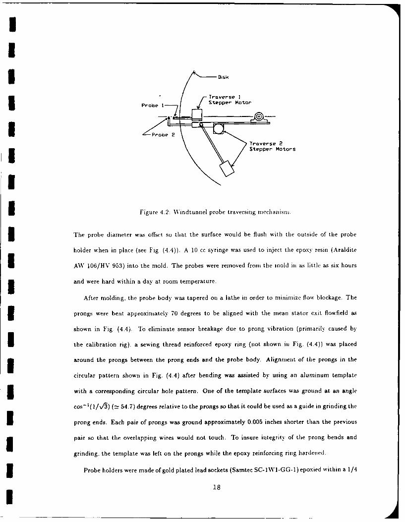
The triple-wire probes used for this study were molded using techniques similar to those of Ukeiley et

Ial. (1990). Tempered steel music wire with a diameter of 0.020 inches was used as prong material.

The prongs were suspended in the mold in order to have an exact match to the probe holder

electrical sockets. Two plexiglass mold halves with the cylindrical probe shape machined into then

i and aluminum end plugs with identical hole patterns for the prong suspension comprised the mold.

17I

I!

I3 Disk

F t raverse I3rb S -7teppe'- Motor

3 Stepper Motors

I Figure 4.2: Winditunnel probe traversing mechanism.

3 The probe diameter was offset so that the surface would be flush with the outside of the probe

holder when in place (see Fig. (4.4)). A 10 cc syringe was used to inject the epoxy resin (Araldite

I AWV 106/HV 953) into the mold. The probes were removed from the mold in as little as six hours

and were hard within a day at room temperature.

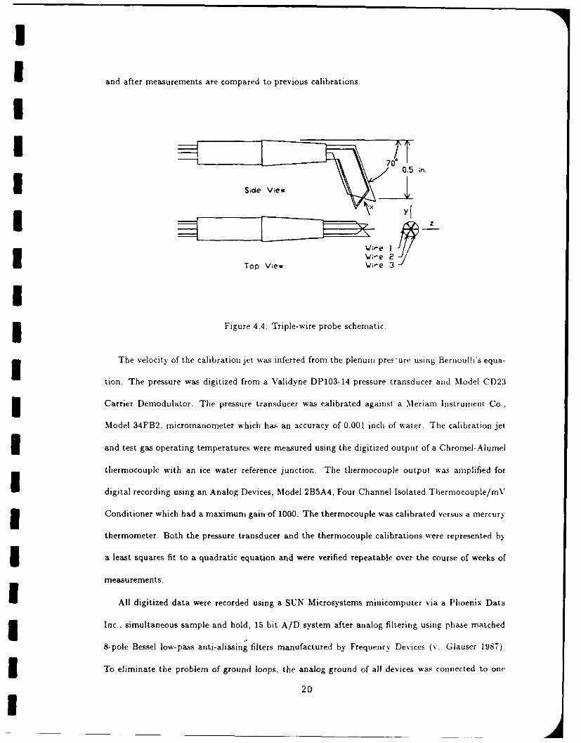
After molding. the probe body was tapered on a lathe in order to minimize flow blockage. The

i prongs were bent approximately 70 degrees to be aligned with the mean stator exit flowfield as

shown in Fig. (4.4). To eliminate sensor breakage due to prong vibration (primarily caused by

i the calibration rig), a sewing thread reinforced epoxy ring (not shown in Fig. (4.4)) was placed

3 around the prongs between the prong ends and the probe body. Alignment of the prongs in the

circular pattern shown in Fig. (4.4) after bending was assisted by using an aluminum template

5 with a corresponding circular hole pattern. One of the template surfaces was ground at an angle

cos-'(1/'/3) (:t 54.7) degrees relative to the prongs so that it could be used as a guide in grinding the

I prong ends. Each pair of prongs was ground approximately 0.005 inches shorter than the previousu pair so that the overlapping wires would not touch. To insure integrity of tile prong bends and

grinding, the template was left on the prongs while the epoxy reinforcing ring hardened.

3 Probe holders were made of gold plated lead sockets (Samtec SC-IW 1-GG-1)epoxied within a 1/4

18

II

I -

UU

Injection HoLe

Prong Hole ProngSpr Support

SuportI

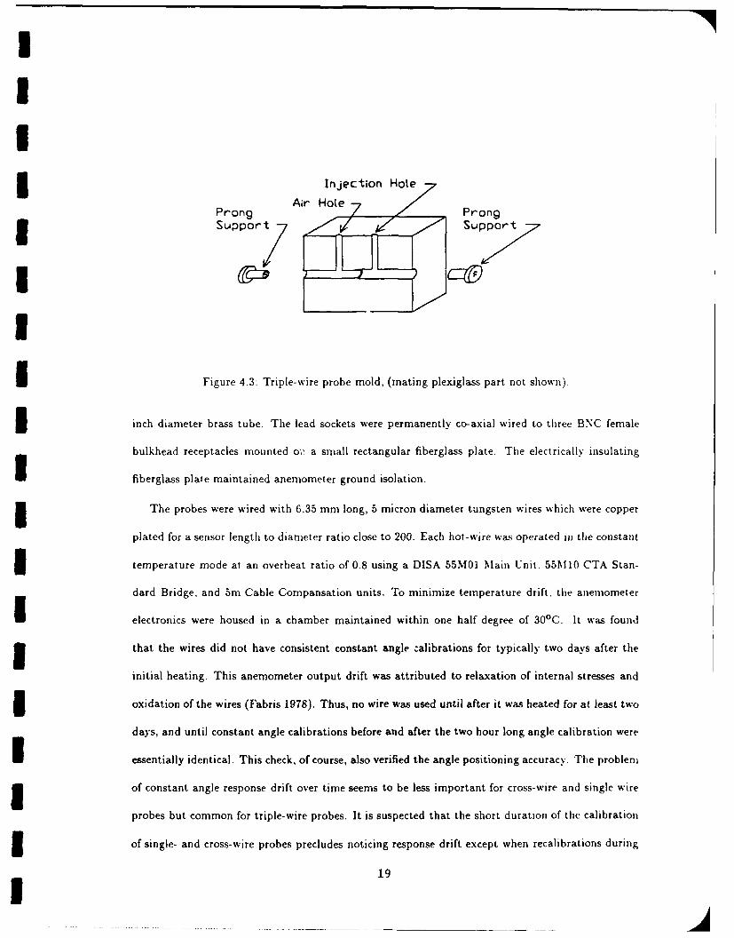
I Figure 4.3: Triple-wire probe mold, (mating plexiglass part not shown).

3 inch diameter brass tube. The lead sockets were permanently co-axial wired to three BNC female

bulkhead receptacles mounted o a small rectangular fiberglass plate. The electrically insulating

I fiberglass plate maintained anemometer ground isolation.

3 The probes were wired with 6.35 mm long, 5 micron diameter tungsten wires which were copper

plated for a sensor length to diameter ratio close to 200. Each hot-wire was operated in the constant

3 temperature mode at an overheat ratio of 0.8 using a DISA 55M01 Main Unit. 55M10 CTA Stan-

dard Bridge, and 5m Cable Compansation units. To minimize temperature drift, the anemometer

electronics were housed in a chamber maintained within one half degree of 30'C. It was found

3 that the wires did not have consistent constant angle zalibrations for typically two days after the

initial heating. This anemometer output drift was attributed to relaxation of internal stresses and

5 oxidation of the wires (Fabris 1978). Thus, no wire was used until after it was heated for at least two

days, and until constant angle calibrations before and after the two hour long angle calibration were

I essentially identical. This check, of course, also verified the angle positioning accuracy. The problem

of constant angle response drift over time seems to be less important for cross-wire and single wire

probes but common for triple-wire probes. It is suspected that the short duration of the calibration

3 of single- and cross-wire probes precludes noticing response drift except when recalibrations during

19

I:

I7

1 and after measurements are compared to previous calibrations.

I

0.5i.

* 2 rI _

\./re2Top View 7 e 3

I5 Figure 4.4: Triple-wire probe schematic.

3 The velocity of the calibration jet was inferred from the plenum pres-ure using Bernouli's equa-

tion. The pressure was digitized from a Validyne D P103-14 pressure transducer and Model CD23

m Carrier Demodulator. The pressure transducer was calibrated against a Meriaml Instrument Co.,

Model 34FB2, micromanometer which has an accuracy of 0.00 1 inch of water. The calibration jet

__ and test gas operating temperatures were measured using the digitized output of a Chrome-Alumel

mm thermocouple with an ice water reference junction. Thle thermocouple output was amplified for

-- digital recording using an Analog Devices, Model 2B5A4, Four Channel Isolated Th~ermnocouple/mV

3 Conditioner which had a maximum gain of 1000. The thermocouple was calibrated ver-sus a mercury

thermometer. Both the pressure transducer and the thermocouple calibrations were represented by

5 a least squares fit to a quadratic equation and were verified repeatable over the course of weeks of

measurements.

I All digitized data were recorded using a SUN Microsystems minicomputer via a Phoenix Data

3 Inc., simultaneous sample and hold, 15 bit A/D system after analog filtering using phase matched

8-pole Bessel low-pass anti-aliasing filters manufactured by Frequency Devices (v. Glauser 197).

3 To eliminate the problem of ground loops, the analog ground of all devices was connected to one

20

Iil Ve

I

I source via a bank of isolated ground electrical receptacles.

I4.3 Sampling Criteria

The A/D used for this study had a maximum sampling rate of 325 KHz which, when divided by the

3 number of channels to be sampled, yields the maximum sampling rate of any of the channels. Using

two triple-wire probes, a pressure transducer and a thermocouple limited the sampling frequency

to just above 40 KHz. The acceptability of this limited sampling frequency was investigated via

3 consideration of the physical limitations imposed by the flow and probe geometry.

The probe dimensions set a restriction or the trequencles of the flow fluctuatioiis due to their

3 spatial filtering. The smallest spatial scale resolvable by a probe is twice the spatial dimensions of

the transducer. This imposes a limit on the freyqaic.es resolvable by the probe ofI Uft =

(4.1)

I where U, is the characteristic mean convective velocity, and It is the characteristic transducer size.

3 In this experiment. 1, = 2 mm and U, : 55 m/s. This would suggest that the measurements should

be low-pass filtered with a 13.8 KHz cutoff frequency before recording due to the limited probe

3 spatial resolution.

Similar to the time scale associated with transducer spatial filtering is that associated with

multiple-probe measurements of eddies. The spatial extent of the eddies simultaneously sensed by

3 two probes is determined by the probe spacing (I.) and the characteristic mean convection velocity

(Uc). Assuming the turbulence field is effectively "frozen" as it passes the probes, the minimum

5 eddy time-scale resolvable by both probes is given by

I = I,, (4.2)

where f, is the associated maximum frequency. For this experiment the apparatus limited the

spacing to 1.4 cm. Thus the maximum resolvable flow frequency was reduced to approximately

3.9 KHz.

21

I

I Preliminary measurements using one triple-wire probe, at 60 KHz while filtering at 25 KHz

were used to determine the extent of the energy content at high frequencies. It was found that

below 5 ti.z, the spectra had approximately one decade of -5/3 character. Above 5 KHz there

was broadband noise which was identified to be a combination of prong and/or wire vibration and

electronic noise at 12 KHz and 16 KHz. The proposed frequency limit set by the minimum probe

spacing was deemed acceptable and so the anti-aliasing filters were set to cut-off at 4 KHz. In order

to more than satisfy the Nyquist criterion, a 10 KHz sampling frequency was then used.

The record length and number of blocks were determined from the integral scale and the statistics

3 required for the ensuing analysis (v. George et al. 1978). The integral scale

3 I = r(i, r)dr (4.3)

can be expressed in terms of the correlation coefficient

- C(£, r)r(x.r) -- (4.4)

where

C(i. ") = [U(i, 1) - u][u(i, I + 7) - 6] (4.5)

is the covariance and

,r2 = C(O) =[,,(,l) - ]2 (4.6)

3 is the variance of the signal u(i, 1). Combining Eqs. (4.4) and (4.3) yields

3 I- fjC(i, r)dr (4.7)Or2

3 For experimental data, it is convenient to calculate the integral scale from the spectrum

ccS(i, f) = C(, r)e--72'fdr (4.8)

which is the Fourier transform of the correlation. Since C(i, r) is even and real, the spectrum is

3 also even and real, so that Eq. (4.8) reduces to

S(i, f) = 2 C(.r)cos27rfrdr (4.9)

3 22

I Since S(O) is exactly twice the integral in Eq. (4.7), the integral scale can be written in the form

I = S(, O) (4.10)2Ur2

The spectrum of the digitized experimental data was found using Eqs. (3.8) and (3.9) as outlined in

Chapter (3). The spectrum at the origin was extrapolated from the first two points of the spectrum

since the dc value was zero for the spectrum of the fluctuations (u(i, t) - U).

The resulting evaluation of Eq. (4.10) yielded an integral scale of approximately 0.6 ms. Thus

recording 1024 samples per record at 10 KHz results in over 100 integral scales per record. Waiting

3 one record length between blocks insured statistical independence of the ensembles. In reality, tl:c

processing of each block increased the interblock temporal spacing to several record lengths.

The accuracy of measurements of statistical quantities such as spectra are dependent on the

number of ensembles used for the estimate. The second order statistics required for the '"OD

implementation can be estimated with good accuracy using 300 or more blocks (v. George et al.

3 1978 and Tan-atichat and George 1985). In light of the computational requirements, the spectral

estimates derived in this study were ensemble averages of 300 individual spectra.I4.4 Hot-Wire Implementation

Calibration of cross and triple-wire probes is commonly performed in two parts: a niuiiaa wire

I calibration of each wire and a subsequent angle calibration. The normal wire calibration consists of

3 a measurement of the wire voltage for many (typically twenty or more, v. Swaminathan, Rankin and

Sridhar 1984) velocities normal to the wire for each wire. A response equation such as a version of

3 King's Law (King 1914, Sidall and Davies 1972) or a polynomial (George et al. 1987) is fit to normal

wire calibration data. The angle calibration data consists of measurements of wire voltages for a

I large range of velocity directions (at a number of velocity magnitudes for low speed applications).

3 The angle calibration voltage data is then converted, via the normal response equation. to effective

normal velocities. The yaw (and sometimes pitch) parameters of an angle response equation (such as

3 Jorgenson's, (1971) or a cosine law (llinze 1959) are then determined using a regression technique.

23

I

I The usual multiple-wire calibration techniques using the aforementioned procedure require the

3 wire angles to be known a priori. Mutually orthogonal wires are often assumed in order to have

an analytical decoding algorithm for triple-wire probes. Orthogonality of cross-wires need not be

assumed in order to have an analytical decoding scheme, however. The errors incurred by calibrating

non-orthogonal triple-wire probes using the response equations assuming mutually orthogonal wires

I may exceed 10% (Lekakis et al. 1989). Successful calibration of non-orthogonal triple-wire probes

has been achieved using sophistocated curve fits (Butler and Wagner 1983) and iterative solutions

to Jorgenson's equations (Lekakis et al. 1989). The analyses discussed by these researchers also

3 requires prior knowledge of the wire angles.

The wire angles of commercially available probes are given only to some known tolerance by the

manufacturers, and independently made or repaired probes have unknown wire angles. Determina-

3 tion of flow-wire orthogonality is consequently determined using optical techniques or maximization

of the anemometer voltage for a given velocity. A calibration method which determines wire angles

3 and yaw factors, without the use of normal wire calibrations, would eliminate a source of error and

save time.

sA calibration method for multiple-wire probes which determines wire angles and yaw factors,

3 without the use of normal wire calibrations was developed. This improved calibration technique,

eliminates the error associated with either wire measurements or assumed wire orthogonality. Ad-

U ditionally, this new method saves time since a constant angle calibration can be performed on all

wires at once in lieu of the traditional normal wire calibrations of each wire. The development of

such a calibration using the modified cosine law (Hinze 1959) is outlined below.

I3 4.4.1 Response Equations

The wire orientations can be expressed in terms of the direction cosines in cartesian coordinates as

3 ti = COS ,1 + COS ,,2 + COS, 3 k. (4.11)

* 24

I

ISimilarly, the normalized velocity is given by

I 0 -

I = cos0i + cos aij + cosak3. (4.12)

3 Taking the dot product of the wire orientation and the normalized velocity yields an expression for

the angle between the flow and each wire orientation (7y) given by

cos % = cos Qj cos 0,. (4.13)j=l

For low speed flows (U < 5m/s) the yaw sensitivity of a hot-wire is largely velocity dependent

(Beuther et al. 1987), and due to the increased relative effect of the prongs for low speed applications,

the pitch sensitivity of the wires comprising the probe is significant (Jorgenson 1971). For high speed

3 flow applications however, the yaw sensitivity of a hot-wire is virtually independent of velocity and

the pitch sensitivity is negligible. Thus for high speed flows (for which the calibration described

3 below was used), Jorgenson's (1974) equations reduce to the modified cosine law of Hinze (1959).

Thus, the angle calibration required for the analysis presented herein can be performed at a velocity

magnitude representative of the application flow speed. The modified cosine law for each wire can

be expressed as( (1)cos-(4.14)

I where Ueff, i is the effective normal velocity of wire i and 7y is the angle between wire i and the

instantaneous velocity. The yaw factor ki account for heat transfer due to the velocity component

along the wire.

3 Substitution of Eq. (4.13) into Eq. (4.14) yields the angle response equation

I~~~ CO 1j CO 3k ) cs i s j (4.15)

Traditional measurements of normal wire and yaw calibration data can be used to determine (via, for

example, a Least Squares optimization) the yaw factors (k,) and the wire orientation angles (Oij).

3 This was the approach used by LeBoeuf and George (1990) for cross-%ire probes and LeBoeuf

(1990) for triple-wire probes. However without prior knowledge of the wire angles and since the

3 implementation flow should never be normal to any of the wires (since it would typically be at too

25

I

N high a yaw angle on other wires) it is advantageous to use constant angle calibrations at known

probe angles without assuming orthogonality to each wire.

The final derivation of the response equations requires the use of a normal wire response equation

such as King's Law (King, 1914) or the more general polynomial (v. George et al., 1987):

R -= Aii (4.16)I 1=0

where, for best accuracy (Beuther 1980), the Reynolds number

Re1 = Ueffidi (4.17)

V

is evaluated at the ambient temperature (T.) and the Nusselt number

Nui- hidi (4.18)ka,l

is evaluated at the film temperature (Tf, = TTj = wire operating temperature). The heat

transfer coefficient (hi) can be eliminated from the Nusselt number in terms of the wire voltage E,I since

hi = i(4.19)

- (Tj. - T.)7rdL, L

and

q,3 / ,. (4.20)

3 The Nusselt number can then be expressed as

Nui = tv,, (4.21)U irRwiLikai(T.,,i - T)

where

I R.i = resistance (4.22)

di = diameter (4.23)

Li = length (4.24)Iand

k, = thermal conductivity of air at the film temperature (4.95)

26

I

I of wire i. The kinematic viscosity (v) is, as noted above, evaluated at the ambient temperature.

3 The unknown wire temperature (T, 1 ) can be eliminated from Eq. (4.21) in terms of known quan-

tities. For constant temperature anemometry (CTA), the wire temperature (T ,,) (and consequently

resistance (R,,)) is constant. The resistance overheat ratio is given by

U= ,j - .°,j (4.26)

where / 0,i is the wire resistance at the setup ambient temperature (T0,o). The wire resistance can

I be expressed to a first approximation as

3Ri = R,,i[1 + a(T., - To)] (4.27)

3 in terms of the temperature coefficient of resistivity (a). Combining Eqs. (4.26) and (4.27) and

solving for the wire resistance yields

T , = a + Ta 0 - (4.28)

Substitution of Eqs. (4.17), (4.21) and (4.28) into Eq. (4.16) yields

,V F RA . :,P , ( -+ T.o - T.)

=0 [ ]The constant wire geometry parameters (d, and L1 ) and the wire resistance (R,.,) can be factored

3 into the polynomial parameters such that the normal wire response equation reduces to

M(Ueff,) = A', (Eoi)1 (4.30)

I 1=0

where

eff,i - (4.31)E.,iE ,, (4.32)

[', = + To - T.)]and

A ,i= ' rR,j,L,)3. (4.33)

3 A fourth order polynomial with p equal to 0.5 has been found to be consistent with the normal

wire data obtained at the Turbulence Research Laboratory (TRL) and hence has been used for this

3 study.

27

I

Combining Eq. (4.30) and Eq. (4.15) and solving for U/v yields

- = (4.34)[1 + (k fz 0 3 (E)] .

- 1)(ZF3 cosaj cos 0,j)2]3

Calibration measurements taken with the flow at a constant angle relative to the probe (represented

by a.7 = 5= constant) can be fit toI=m=f~ )i, (El,) 1(4.35)

I where 1=0

A l [ + (k - l (4.36)I1)(E3=1 coj COS 0"7)21

and

= L .'ej" (4.37)

The effective skewed (instead of normal) velocity, Ueffj is the velocity magnitude at the angle

3

= Zcosicos j (4.38)j=1

with respect to the wire, which would give the same wire response voltage as the true velocity.

The relationship between the effective normal velocity and the effective skewed velocity can be

derived by combining Eqs. (4.30). (4.35) and (4.36):

UefI', = U 11ef,4 [1 + (k2 - 1)( E cos&3 cosi31 j)2 3 (4.39)j=

The final angle response equation can be found by substituting Eq. (4.39) into Eq.(4.15) and rear-

ranging to get

The calibration parameters in this equation include in addition to the yaw factor (k,), the wire

direction cosines (jj). The data required for such a calibration consist of constant angle calibration

data (analogous to normal wire data) and yaw angle calibration measurements which are described

in a later section.

If the fluid temperature is assumed constant, then the coefficients of Eq. (4.30) would absorb

the temperature dependent factors of Eqs. (4.31) and (4.32) and all primed quantities except A,

* 28

*I in the preceding analysis would be equal to their unprimed counterparts. A common argument for

assuming isothermal flow is that the test flow is left running long before beginning the experiment

so that thermal equilibrium is reached. Caution is recommended regarding such an assumption

however, since the calibration flow (whether in the test facility or a separate calibration facility)

is probably not at the same temperature as the test flow during the experiment. In this study for

I example, the calibration jet temperature was found to be a function of both the blower running time

and the blower speed and would vary by as much as 2°C over the ourse of a single constant angle

calibration.

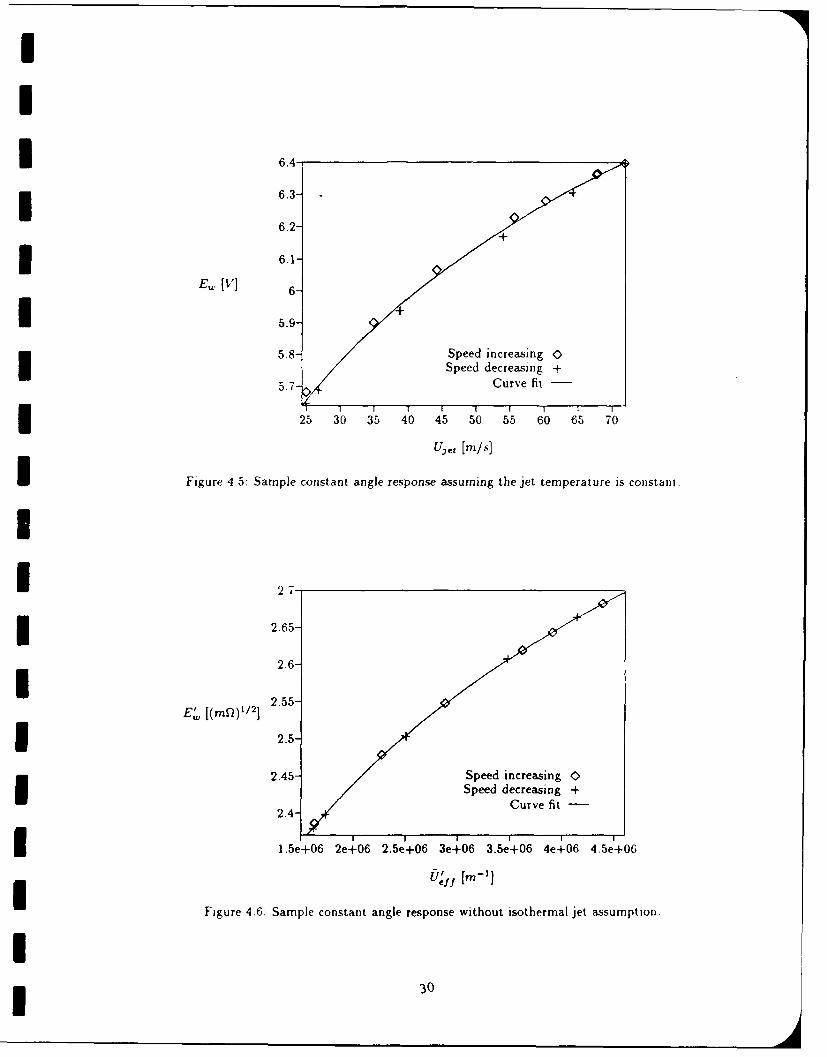
3 To exemplify the potential problems regarding an isothermal calibration assumption, a small

set of constant angle calibration measurements were recorded and fit with Eq. (4.35) and with the

I polynomial response equation

4

U,e = AIE.' (4.41)1=0

for isothermal flow. The calibration set was unusual since the blower speed was increased between

half of the data points and without shutting down, decreased between the second half of the data

points. For the same jet velocity, the temperature of the airstream was higher for the second half of

the calibration ddta than for the first half of the data. The results of a least squares fit to Eq. (4.41)

3 is shown in Fig. (4.5). The effect of the jet temperature change resulted in curve fit errors up to 3.8%.

The least squares fit of Eq. (4.35) for the same data is shown in Fig. (4.6) with a maximum error

of 1.2%. The collapse of the data is remarkably good, contrary to some researchers condemnation

of relationships between Nusselt and Reynolds numbers for practical hot-wire use (Bruun 1979).

The assumption of isot. _rmal flow was therefore not used for this study and Eq. (4.35) was used to

I model the wire voltage response to the effective skewed velocity.

4.4.2 Parameter Optimization

The optimized calibration parameters based on the method of Least Squares are determined by

minimizing the functions

I 0, = (Y, - F,(X,))TW(y, - F,(Xi)) (4.42)

* 29

*6 .4~

* 6.3-

6.2-1 6.1-+

E., [V] 6-

5.9-

5.8- Speed increasing tZSpeed decreasing +

5.7 Curve fit

25 30 35 40 45 50 55 60 65 70

Uj- [m/s1

I Figure 4.5: Sample constant angle response assuming the jet temperature is constant.

2.65-

2.6-

1 2.5-

2.45- Speed increasing o)Speed decreasing +

2.4] Curve fit'

I1.5e+06 2e+06 2.5e'+06 3e+06 3.5e+06 4e+06 4.5e+06

Figure 4.6; Sample constant angle response without isothermal jet assumption.

* 30

Ii

i for each wire i. The superscript T indicates transpose, For the wire angles to be physically consistent

the direction cosines of each wire orientation must satisfy

33:cos2i3,. = 1. (4.43)

j=l

3 This constraint was applied numerically by including it with the N data pairs in the definitions of

Yi and Fj such that

I (~)2

i Y 2 = (4.44)

* N

and

1,+(X.,-1)( = co o,X,.,)2

Fj (4A45)

U = i

i which is a function of the parameter vector

cos I3,

i cos /3,2

COS fli,3=i CSP, (4.46)

for each wire i. A diagonal weight matrix (W) is appropriate for this application. The first N entries

of W can in general be set to unity. To deweight high uncertainty data 1however, the corrresponding

3 weight can be set lower. In order to numerically apply the constraint of Eq. (4.43), the last entry

of W can be set larger than the weighting of the data. Unity constraint weighting was found to be

sufficient however, so that in general the weight matrix can be set equal to the identity matrix.

I 31

I

I If the data and model vectors are redefined to be

Yi= 2 (4.47)

Iand

u 2 f 1+(X2.,-)(Z3 CoSo,X.,)4

2

I -+(x.-)(E ., ,s &,,x.,)2)

Ij 2 _1+ __.2 __C.____,) (4.48)

i =l I i2

respectively, then a minimization of the sum squared relative error is performed. This was deemed

more appropriate since it produces a more uniform fit for a larger range of flow angles.

The non-linear Least Squares data fit defined by Eq. (4.42) through (4.46) (or Eqs. (4.46) through

3 (4.48) can be solved by Gaussian Least Squares Differential Correction (GLSDC) (see for example

Junkins, 1987). The complexity of the optimization, however, necessitates the use of a gradient

search prior to applying GLSDC if the initial parameter vector deviates too much from the optimum.

3 The following iteration comprises the GLSDC calculation.

Xi = (AT WAi)-ATW6YI + X,.d (4.49)

3 whereOaFj

A, = 8 X.. (4.50)

and

I 6Yi = Yi - Fi 'X.,, (4.51)

I The superscript -1 indicates matrix inversion. The parameter vector Xc,d must be initialized to

perform the first iteration and subsequently is the result of the prior iteration.

3 Due to the extreme nonlinearity of the response function, Eq. (4.49) resulted in an increase in

the cost function (Eq. (4.42)) for some values of X1 ,od. To overcome such an increase, the iterative

I correction to Xi was relaxed as illustrated by Eq. (4.52).

Xi = R(AT WA,)-'ATW6 Y, + Xi,ad (4.52)

* 32

I

The relaxation parameter (R) was decrease by a factor of two until the cost function decreased for

a given Xi,dd, then update of the parameter vector was performed.

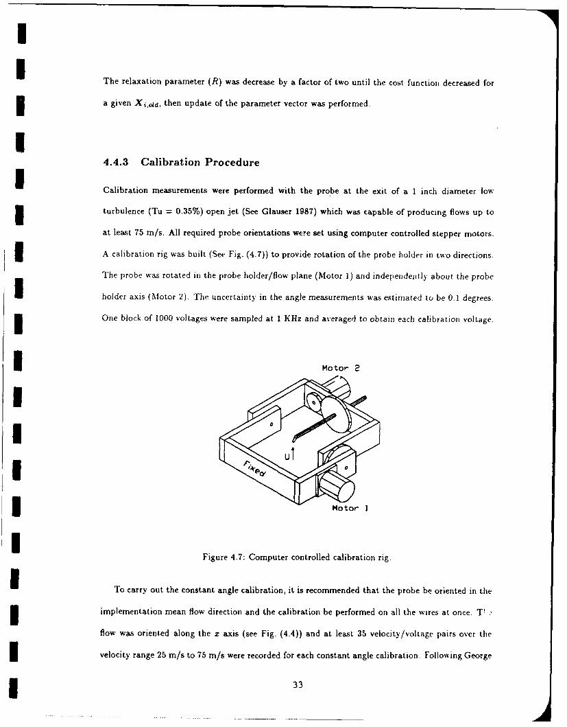
I4.4.3 Calibration Procedure

i Calibration measurements were performed with the probe at the exit of a 1 inch diameter low

turbulence (Tu = 0.35%) open jet (See Glauser 1987) which was capable of producing flows up to

at least 75 m/s. All required probe orientations were set using computer controlled stepper motors.

A calibration rig was built (See Fig. (4.7)) to provide rotation of the probe holder in two directions.

The probe was rotated in the probe holder/flow plane (Motor 1) and independentl] about the probe

holder axis (Motor 2). The uncertainty in the angle measurements was estimated to be 0.1 degrees.

One block of 1000 voltages were sampled at 1 KHz and averaged to obtain each calibration voltage.

3 Motor 2I

UUI Motor I

Figure 4.7: Computer controlled calibration rig.

- To carry out the constant angle calibration, it is recommended that the probe be oriented in the

3 implementation mean flow direction and the calibration be performed on all the wires at once. T' ."

flow was oriented along the z axis (see Fig. (4.4)) and at least 35 velocity/voltage pairs over the

velocity range 25 m/s to 75 m/s were recorded for each constant angle calibration. Following George

1 33

I

I et al. (1987), a fourth order polynomial response equation was used to relate the wire voltages to

the effective skewed velocities (Eq. (4.35). The kinematic viscosity (v) and thermal conductivity

(k0,i) required for the evaluation of U,'ff (via Eq. (4.37)) and E'efl, (via Eq. (4.32)) were obtained

using a quadratic interpolation at the measured air or film temperature. The tabulated properties

used for the interpolation were those of Touiutikian et al. (1975) and Touloukian, et al. (1970). The

parameters of the calibration (A',i ,...., A') were determined for each wire i using a linear least

squares fit. Typically the wires used for this study had maximum constant angle calibration curve

fit errors less than 0.5%.

For high velocity applications (the topic of this paper), the yaw angle calibration consists of

recording the voltage of each wire for a number of probe orientations while the probe is exposed to a

3 flow representative of the maximum application velocity. Angle calibration data was obtained with

the probe exposed to nearly constant (but not assumed so) velocity flow at approximately 60 m/s.

The probe was rotated about the probe holder and swept through the probe holder/flowN' direction

3 plane in 5 degree increments. For each probe orientation, the jet velocity and the wire voltages

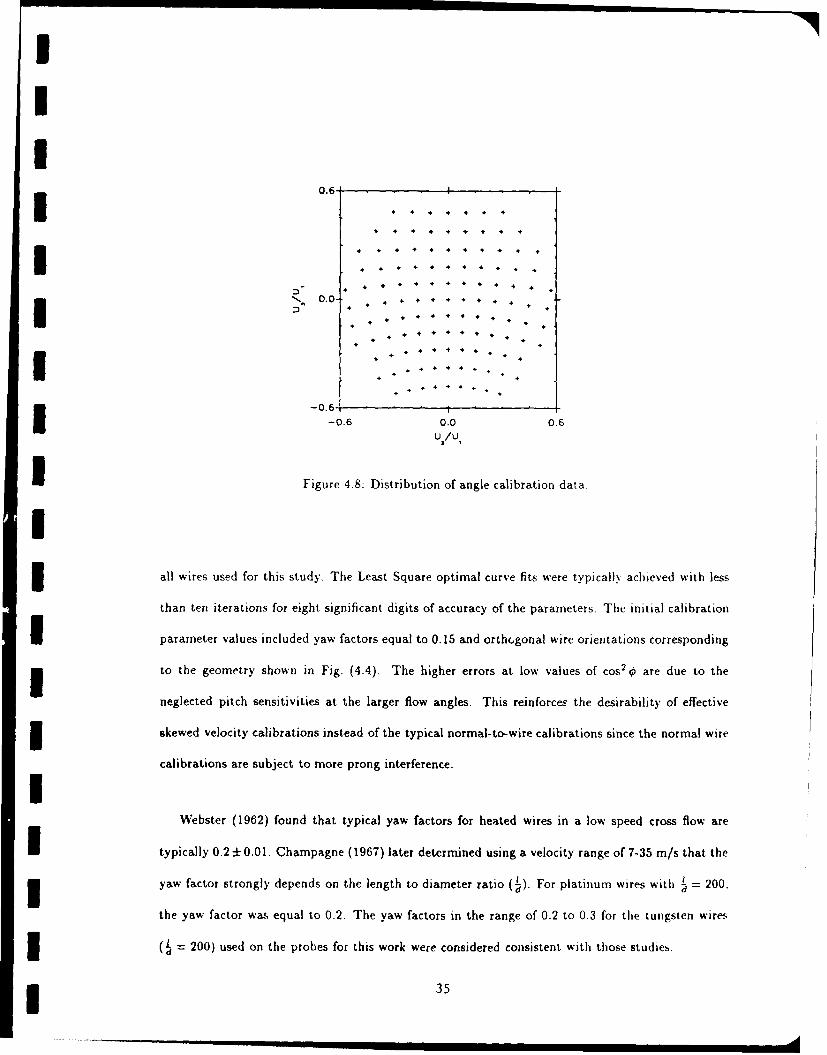
were recorded. The resulting 124 measurement directions are indicated on Fig. (4.8) as a plot of U

versus 4 in which a circle of radius tan 30 ' (-- 0.6) would encompasses all velocity vectors within a

30 (,:gree cone aligned with the x axis. The angle calibration data was used in conjunction with the

I constant angle response to obtain values of Ueff,i/U which were modeled by Eq. (4.40) as described

* above.

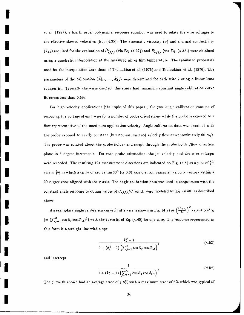
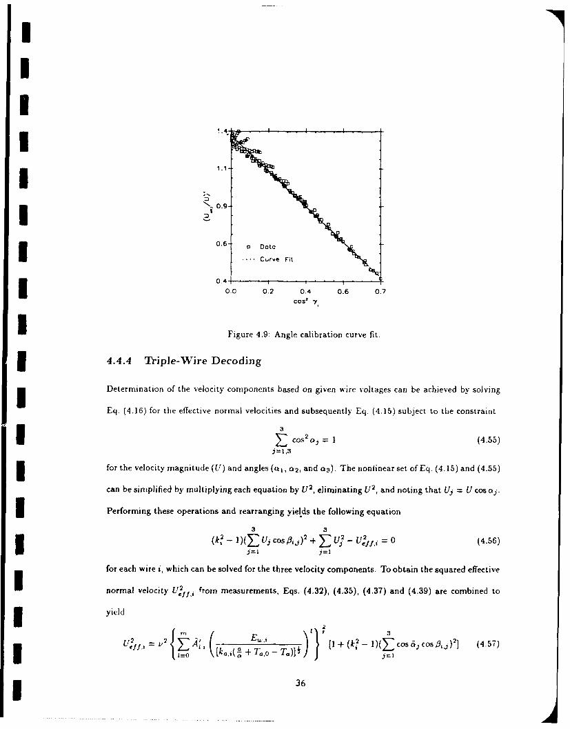
An exemplary angle calibration curve fit of a wire is shown in Fig. (4.9) as (U) versus cos2 "h

(= 1 cos &j cos/3,j) 2 ) with the curve fit of Eq. (4.40) for one wire. The response represented in

this form is a straight line with slope

k, - 1 2(4.53)1 + (k~ -1_) (E3 ICOS 6j O 0.

and intercept

I1 (4 54)

The curve fit shown had an average error of 1.6% with a maximum error of 6% which was typical of

i 314

II

0.6

U~~ 4 .

I* 4* • 4 4 4

, , . .... 4 . ...

0.0. * . . * .

+ 4 +

4 4

+. 4 + 4 , +

+ 4

-0.61-0.6 0.0 0.6

U /U

IFigure 4.8: Distribution of angle calibration data.

all wires used for this study. The Least Square optimal curve fits were typically achieved with less

than ten iterations for eight significant digits of accuracy of the parameters. The initial calibration

I parameter values included yaw factors equal to 0.15 and orthcrgonal wire orientations corresponding

to the geometry shown in Fig. (4.4). The higher errors at low values of cos2 0 are due to the

neglected pitch sensitivities at the larger flow angles. This reinforces the desirability of effective

3 skewed velocity calibrations instead of the typical normal-to-wire calibrations since the normal wire

calibrations are subject to more prong interference.

Webster (1962) found that typical yaw factors for heated wires in a low speed cross flow are

U typically 0.2 ± 0.01. Champagne (1967) later determined using a velocity range of 7-35 m/s that the

3 yaw factor strongly depends on the length to diameter ratio (i). For platinum wires with 1 = 200,

the yaw factor was equal to 0.2. The yaw factors in the range of 0.2 to 0.3 for the tungsten wires

d( = 200) used on the probes for this work were considered consistent with those studies.

I.l 35

U4I

I~ 11

I

1 0.6- Data

Curve Fit

0-4-

0.0 0.2 0.4 0.6 0.7I Cos' 7Y

Figure 4.9: Angle calibration curve fit.

3 I4.4.4 Triple-Wire Decoding

u Determination of the velocity components based on given wire voltages can be achieved by solving

Eq. (4.16) for the effective normal velocities and subsequently Eq. (4.15) subject to the constraint

> cos 2 a = 1 (4.55)ft , ,3

for the velocity magnitude (U) and angles (a1, a2, and a3). The nonlinear set of Eq. (4.15) and (4.55)

can be simplified by multiplying each equation by U2 , eliminating U 2, and noting that U, = U cos as

3 Performing these operations and rearranging yields the following equation

3 3I(k,2- 1)( UffCos P42

+ u- u 2 =0 (4.56)

for each wire i, which can be solved for the three velocity components. To obtain the squared effective

I normal velocity Ue2 .tI from measurements, Eqs. (4.32), (4.35), (4.37) and (4.39) are combined to

* yield

i= ~ 2{ k fAt ,(, +Tl1T)

)} + (k - )( 3cos 6 ,cos B,j)2 ] (4.57)

eff,t V3 2 C&O6(.=o [k.,i( + T.o [I +o J

k i =,

. . . . . . . .. . . .. .

. . . ... . .. . .. . . . .. . . .. . . . . ... . .. . . . .... ... . .. .. . ..

362

I

I where all quantities on the right hand side are known once measurements of E,,,i are aquired.

The nonuniqueness of the solutions to the nonlinear equation set (4.56) (examined in detail by

Lekakis et al. (1989)) can be overcome by orienting the probe in the mean flow direction such that

the velocity vector fits within a cone containing only one solution to these equations. This overcomes

the ambiguity associated with the axisymmetry of the wires. Requiring the flow to remain within a

I certain range of angles of course limits the turbulence intensities acceptable during implementation.

The problem of rectification (the mapping to the presumed solution quadrant of velocities outside

that quadrant) has been studied by Andreopoulos (1983). Andreopoulos (1983) determined, using

simulated data, that a reasonable limit for the turbulence intensity is 30% in order to minimize the

statistical effects of rectification. The flow under consideration here had a maximum turbulence

3 intensity well below the 30% proposed bound.

Successive approximation was demonstrated for Jorgenson's equations (1971) in essentially the

form of Eq. (4.56) by Andreopoulos (1983). Successive approximation was determined to be an

I unstable solution technique for this application however, even with the coordinate axes oriented

such that the velocity components were all the same sign (as suggested in private communication).

3 In fact, several methods of successive substitution were attempted only to prove ustable also. Because

of its stability, Newton's method was implemented for the solution of Eq (4.56). Typically three

or four iterations were required to achieve four decimal (five or six digit) accuracy when the last

* velocity components were used as the initial iterate.

IIUII

I

5 Preliminary MeasurementsIPreliminary measurements were performed in order to establish the average flow conditions in the

newly developed windtunnel. Time averaged inlet and exit flowfield and airfoil surface static pres-

3 sures were included in these measurements. Inlet flow measurements consisted of average streamwise

velocity at eleven spanwise locations at each of four pitchwise locations. A cross-wire probe was used

3 to perform unsteady two component velocity measurements of the exit flowfield. The cross-wire mea-

surements were used to determine the spatial distribution of Reynolds stresses and local turbulence

U intensity. The exit flowfield was also traversed with a five-hole pressure probe over one vane pitch

in order to measure total pressure, static pressure, and velocity.

3 5.1 Inlet Flowfield

The time averaged streamwise velocity measurements were obtained with a single hot-wire in a plane

23% axial chord upstream of the stator leading edge at 11 spanwise locations for each of four pitchwise

locations. The results, normalized by the mean streamwise velocity have been plotted as spanwise

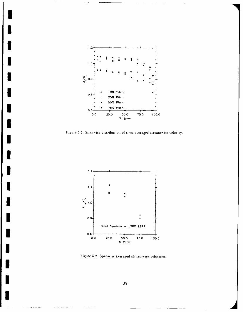
distributions in Fig. (5.1). The inlet flow was found to be nearly uniform over approximately sixty

3 percent of the span at each of the four pitch locations. The hub boundary layer .as less than

five percent of the span while the shroud boundary layer appears to include ten percent of the

I span. This difference in boundary layer thickness is due to the significantly longer shroud entrance

duct compared to the hub nose cone development length (see Fig. (4.1)). The short inlet duct and

lack of flow conditioners upstream of the test section is apparently responsible for the differences

I between the velocity distributions shown in Fig. (5.1) and those reported by Dring et al. (1986).

The measurements of Dring et al. (1986) at the same locations relative to the airfoil leading edge

3 plane are nearly uniform over approximately ninety percent of the span at each pitch location and

do not intersect as the results of this study indicate. In spite of these differences in the spanwise

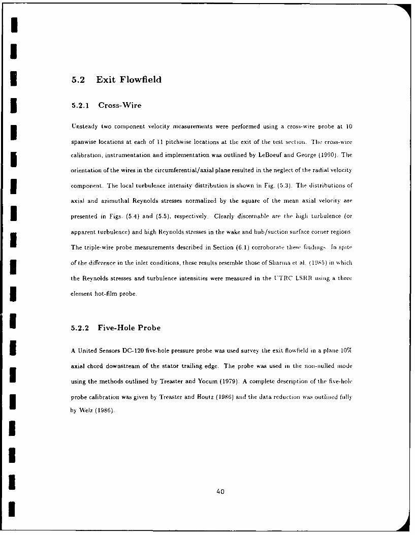
distributions of streamwise velocity, the spanwise averaged streamwise velocities plotted in Fig. (5.2)

along with the results of Dring et al. 1986) indicate identical trends but different magnitudes.

I38 ,

II

1.2 I I

1.1 a

U 0

0.9

o 0% Pitch0.8-

a 25% Pitch

50% Pitch

75% Pitch

0.0 25.0 50.0 75.0 100.0

X Spon

Figure 5.1: Spanwise distribution of time averaged streamwise velocity.

I

1.2-

U.U

I ~1.1- a

I 1.0-

I 0.9

Solid Symbols - UTRC LSRR

0.8 • , i , I

0.0 25.0 50.0 75.0 100.0

X Pitch

Figure 5.2: Spanwise averaged streamwise velocities.

I39

II

I 5.2 Exit Flowfield

5.2.1 Cross-Wire

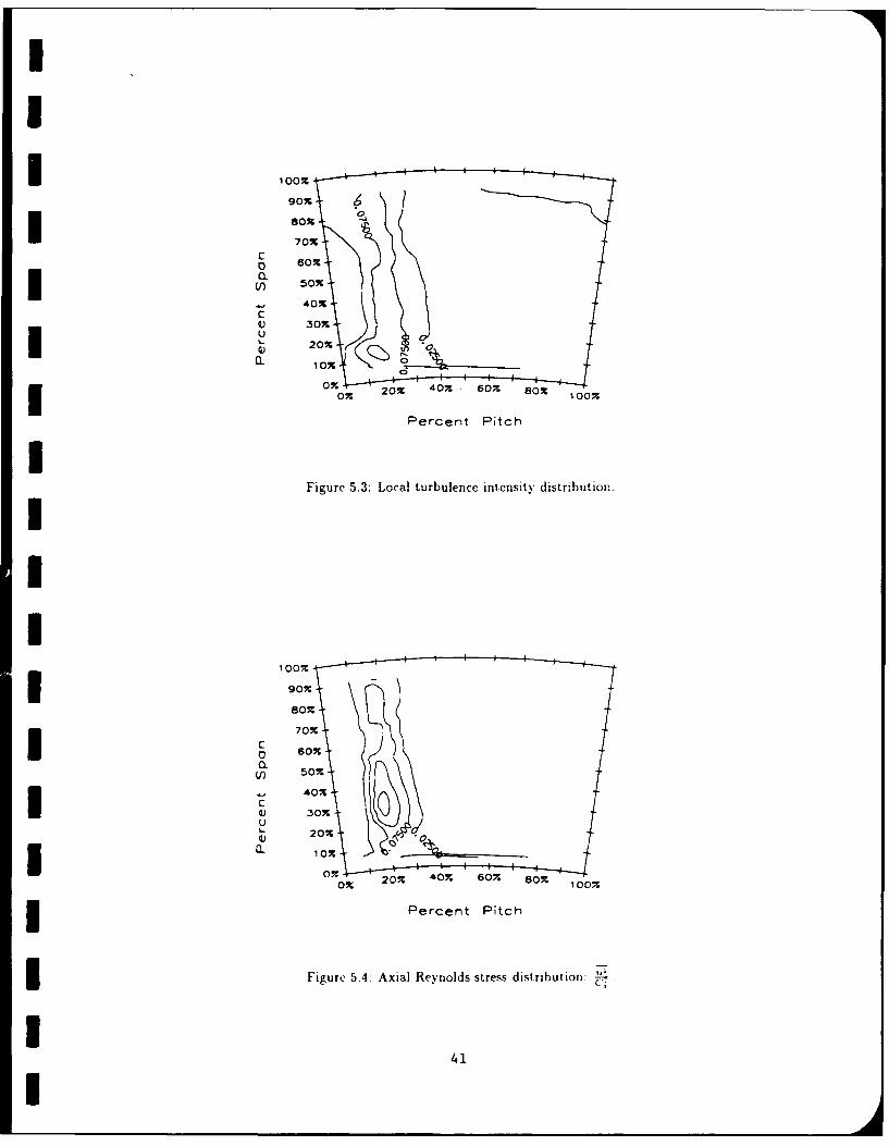
Unsteady two component velocity measurements were performed using a cross-wire probe at 10

spanwise locations at each of 11 pitchwise locations at the exit of the test section. Tile cross-wire

I calibration, instrumentation and implementation was outlined by LeBoeuf and George (1990). The

orientation of the wires in the circumferential/axial plane resulted in the neglect of the radial velocity

component. The local turbulence intensity distribution is shown in Fig. (5.3). The distributions of

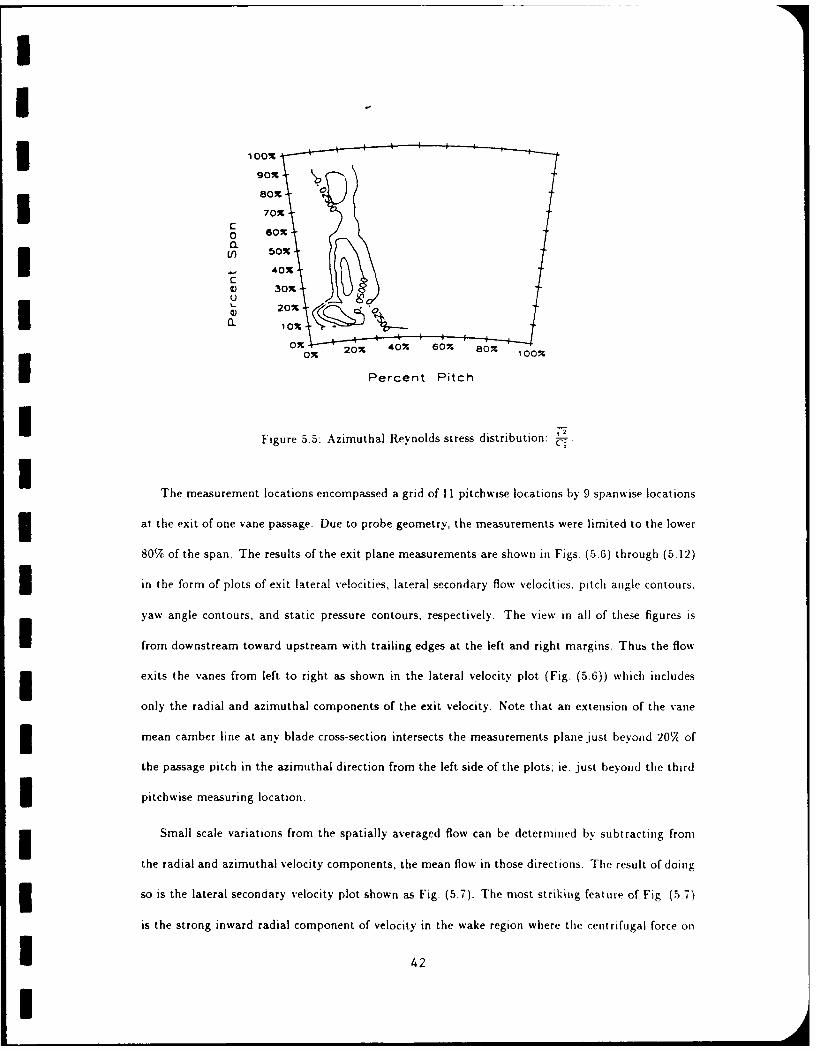
axial and azimuthal Reynolds stresses normalized by the square of the mean axial velocity are

I presented in Figs. (5.4) and (5.5), respectively. Clearly discernable are the high turbulence (or

apparent turbulence) and high Reynolds stresses in the wake and hub/suction surface corner regions.

The triple-wire probe measurements described in Section (6.1) corroboratte these finding-- In spite

3 of the difference in the inlet conditions, these results resemble those of Sharina et al. (19S5) in which

the Reynolds stresses and turbulence intensities were measured in the UTRC LSRR using a three

I element hot-film probe.

1 5.2.2 Five-Hole Probe

I A United Sensors DC-120 five-hole pressure probe was used survey the exit flowfield in a plane 10(

axial chord downstream of the stator trailing edge. The probe was used in the non-nulled mode

using the methods outlined by Treaster and Yocum (1979). A complete description of the five-hole

3 probe calibration was given by Treaster and Houtz (1986) and the data reduction was outlined fully

by Welz (1986).

III 40

I

I 100%

C3 a OCLIr 50%

20 400X% 0

10% 10

Percent Pitch

Figure 5.3: Local turbulence intensity distribution.

100%

V 5 0% 2% 4% 6% 5% 10

1041on4I 0%8%10

I

I

i80%

70Z

C

P 601

% 20 40. 60. 80% 101 Percent Pitch

Figure 5.5: Azimuthal Reynolds stress distribution:

I

The measurement locations encompassed a grid of 11 pitchwise locations by 9 spanwise locations

at the exit of one vane passage. Due to probe geometry, the measurements were limited to the lower

8017 of the span. The results of the exit plane measurements are shown in Figs. (5.6) through (5-12)

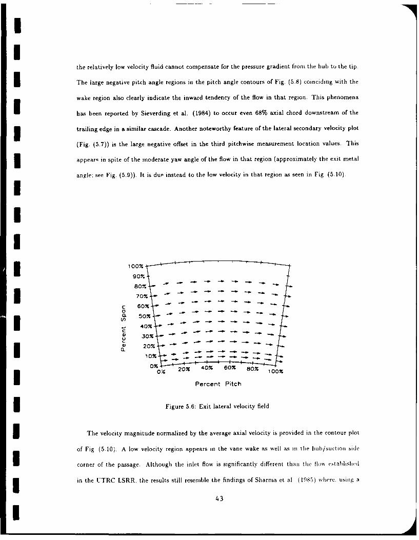
in the form of plots of exit lateral velocities, lateral secondary flow velocities, pitch angle contours.

yaw angle contours, and static pressure contours, respectively. The viewv in all of these figures is

I from downstream toward upstream with trailing edges at the left and right margins. Thus the flow

exits the vanes from left to right as shown in the lateral velocity plot (Fig. (5.6)) which includes

only the radial and azimuthal components of the exit velocity. Note that an extension of the vane

mean camber line at any blade cross-section intersects the measurements plane just beyond 20(7 of

the passage pitch in the azimuthal direction from the left side of the plots; ie. just beyond the third

pitchwise measuring location.

Small scale variations from the spatially averaged flow can be determined by subtracting from

the radial and azimuthal velocity components, the mean flow in those directions. The result of doing

3 so is the lateral secondary velocity plot shown as Fig. (5.7). The most striking feature of Fig (5.7)

is the strong inward radial component of velocity in the wake region where the centrifugal force on

*0 42

I

II

the relatively low velocity fluid cannot compensate for the pressure gradient from the hub to the tip.

l The large negative pitch angle regions in the pitch angle contours of Fig. (5.8) coinciding with the

wake region also clearly indicate the inward tendency of the flow in that region. This phenomena

has been reported by Sieverding et al. (1984) to occur even 68% axial chord downstream of the

3 trailing edge in a similar cascade. Another noteworthy feature of the lateral secondary velocity plot

(Fig. (5.7)) is the large negative offset in the third pitchwise measurement location values. This

appearq in spite of the moderate yaw angle of the flow in that region (approximately the exit metal

angle; see Fig. (5.9)). It is due instead to the low velocity in that region as seen in Fig. (5.10).III

* 100%

70%' .

c 60%- "

0

I t n I -U 30

20 40% 60% 80%0 3Percent Pitch

I Figure 5.6: Exit lateral velocity field.

I The velocity magnitude normalized by the average axial velocity is provided in the contour plot

of Fig. (5.10). A low velocity region appears in the vane wake as well as in the hub/suction side

corner of the passage. Although the inlet flow is significantly different than the flow estahlished

I in the UTRC LSRR, the results still resemble the findings of Sharma et al (1985) where. using a

43I

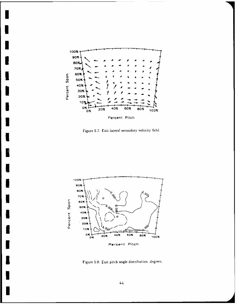
I A

0%

0% 07. 207. 40% 60%. 807. 101 Percent Pitch

Figure 5.7: Exit lateral secondary velocity field.

100%:

BOX

80

70I0C

X 0 0 O O

Percent Pitch

I Figure -5.8: Exit pitch angle distribution, degrees.

44

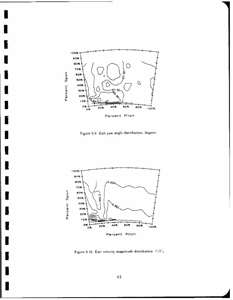
ox~

0X

U 4Oox 67.5

5 Percent Pitch

Figure 5.9: Exit yaw angle distribution, degrees.

C 0

40

C

I 2O~40X G~2sX

Percent Pitch

Figure 5.10: Exit velocity magnitude distribution: I/C',.

45

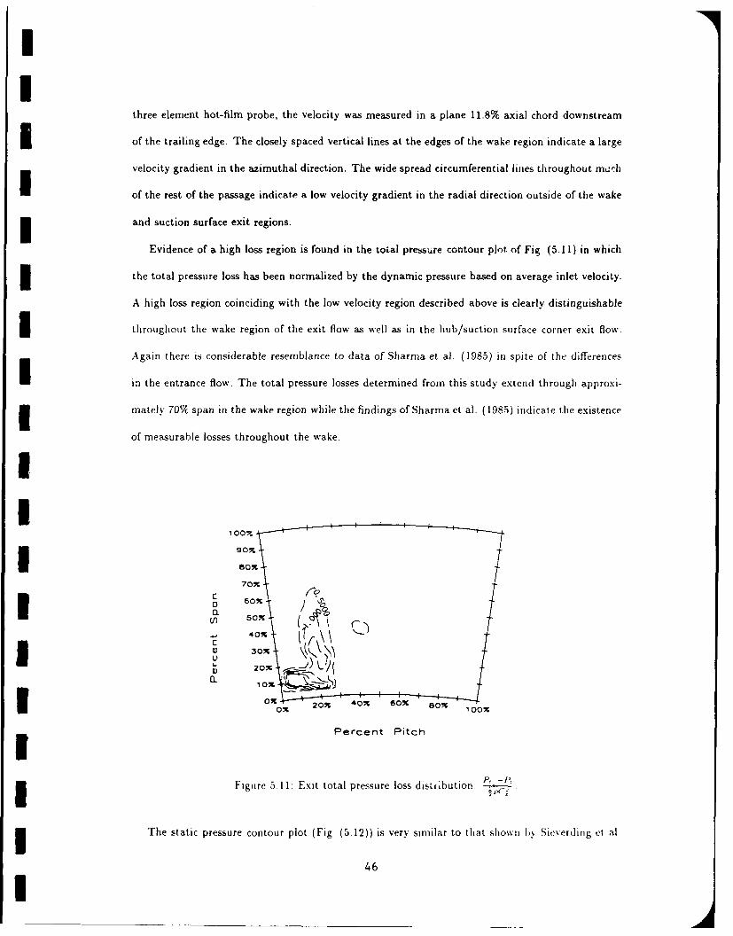
I

three element hot-film probe, the velocity was measured in a plane 11.8% axial chord downstream

of the trailing edge. The closely spaced vertical lines at the edges of the wake region indicate a large

velocity gradient in the azimuthal direction. The wide spread circumferential lines throughout mt:ei

of the rest of the passage indicate a low velocity gradient in the radial direction outside of the wake

I and suction surface exit regions.

Evidence of a high loss region is found in the total pressure contour plot of Fig (5.11) in which

3 the total pressure loss has been normalized by the dynamic pressure based on average inlet velocity.

A high loss region coinciding with the low velocity region described above is clearly distinguishable

I throughout the wake region of the exit flow as well as in the hub/suction surface corner exit flow.

Again there is considerable resemblance to data of Sharma et al. (1985) in spite of the differences

in the entrance flow. The total pressure losses determined from this study extend through approxi-

3 mately 70% span in the wake region while the findings of Sharma et al. (1985) indicate the existence

of measurable losses throughout the wake.

!I

100

70%

0 60% --I a0 o %

I U

OIa 20 40XI 60% 8o 1 00%

Percent Pitch

I Figure 5.11: Exit total pressure loss disLribution: PI -P

3 The static pressure contour plot (Fig. (5.12)) is very similar to that shown b Sieverding et al

46U

I

(1984) at a plane 11% axial chord downstream of the trailing edge of a similar cascade. A large static

pressure gradient into the wake region from the surrounding flow exists at this axial location. There

is evidence in the measurements of Sieverding et al. (1984) that this high azimuthal gradient in

static pressure will be rapidly nearly eliminated downstream of this location leaving predominately

a radial pressure gradient similar to that which appears outside of the wake region in Fig. (5.12).

I

V) 5o0r

-UU

io

20%- 40% 60% 80 1

Percent Pitch

I •Figure 5.12: Exit static pressure distribution: P-

* 5.3 Airfoil Surface Static Pressure Distributions

3 One airfoil was instrumented with static pressure ports at twenty-two locations at each of seven

equispaced spanwise locations. The pressure ports consisted of 0.0135 inch holes drilled normal to

I the airfoil surface into 1/16 inch holes drilled 1/16 inch below the surface. The latter pairs of holes

were connected to an anemometer bank inclined 30 degrees. Pressure taps located at 0.125. 0.25 and

0.375 percent span were connected to the hub access holes while those located at 0.5. 0.625, 0.75 and

3 0.875 percent span were connected to the shroud access holes. A thin transparent tape was used to

47

II

seal off the pressure ports at all spanwise locations except the two (one with access via the hub, and

I the other with access via the shroud) spanwise locations being investigated Z, :,cgoy-Smith and

Graves, 1983).

The resulting pressure coefficient distributions for each spanwise location are shown in Figs. (5.13)

through (5.20). The gross features of each pressure coefficient distribution are alike. The midspan

distribution is shown in Figs. (5.16) and (5.17) together with the results of Dring et al. (1986)

for an axial spacing between the rotor and stator of 50% axial chord and flow coefficients of 68%

and 96% respectively. There was good agreement between the results of this study and those of

Dring et al. (1986) although the suction surface coefficients of pressure found here were higher than

those determined in the LSRR. This could possibly be due to the downstream conditions since no

rotor was used at the stator exit in this study. The significant effect of the rotor on the stator

pressure distribution, especially the suction surface, has been shown by Dring et al (1982) where

the unsteady pressure envelope of the stator in the presence of the rotor was presented.

I

1.20 I I

30

(L 0.3,0-0

I

045P

. 0

00

Io. -0.30- a

0 0o

o Pressure Surface

o Suction Surface-1.80" " " " ' " " " "

0.00 0.25 0.50 0.75 1.00

X/BX

Figure 5.13: Airfoil static pressure distribution at 12.57( span.

I48

I1I

1.20 a a

a

< 0. 0a.n a

0. -0.30-

0 a

0 00

0a. 0

U -1.05-

3 a Pressure Surface

0 Suction Surface

-1.80 -3 0.00 0.25 0.50 0.75 1.00X/Bx

3 Figure 5.14: Airfoil static pressure distribution at 25% span.

I1.20 -3 (3

a0. aI 0.45-

0n a0_ -0.30-

a.aI __, 0

0 0

- 1.05-o Pressure Surface" Suction Surface

0.00 0.25 0.50 0.75 1.00X/BX

I Figure 5.15: Airfoil static pressure distribution at 37.57 span

449U

11.20

I- 0.45-

0. aI 6

0. o '8S 0

0.

ia Pressure Surface

o -1.05- o Suction Surface

a Pressure Surface, LSRR

Suction Surface, LSRR- 1.80 0 " I ' ' -i " " "

0.00 0.25 0.50 0.75 1.00Ix/Bx

Figure 5.16: Airfoil static pressure distribution at 50% span. Included are the results of Dring et al.

I (1987) for V, 0.68.

13 1.20 I . I

0.45-0. 0

0 a(L -0.30- 0*

Pressure Surface

LU - 1.05- 0 Suction Surface

0 Pressure Surface, LSRR

0 Suction Surface. LSRR-1,80O 1

0.00 0.25 0.50 0.75 1.00X/BX

Figure 5.17: Airfoil static pressure distribution at 50% span. Included are the results of Dring et al

I (1987) for 4 = 0.96.

I50i

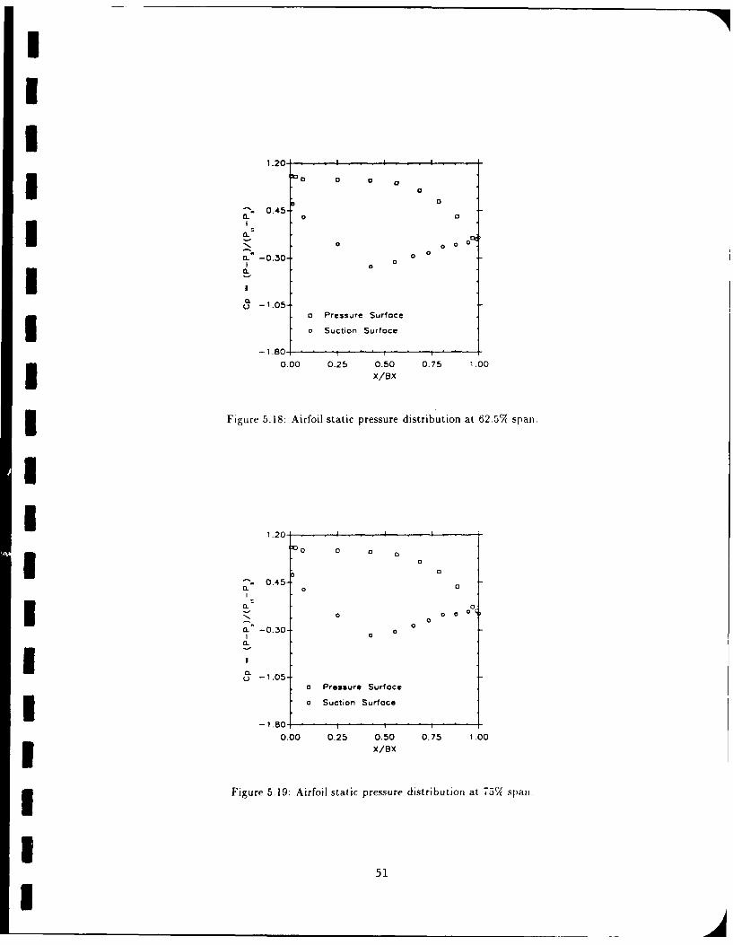
II

1.20 . . . I. I I. . .5 a a a o

0

-6 0.45-|:a. o a

<.0 0 0 0

a. -0.30- 0

Ia.u -1.05-

a Pressure Surface

. 1 Suction Surface

-1.80 ' ' ' " " " ' " "

0.00 0.25 0.50 0.75 1.00X/BX

m Figure 5.18: Airfoil static pressure distribution at 62.57( span.

1I.20 __________. ___. ___ .

1.20 I o

a

0.45-. a

0. o

n. -0.30- 0I o

U -1.05-a Pressure Surface

m Suction Surface

-1.80 . . . i 1 .0.00 0.25 0.50 0.75 1.0

X/BX

UFigure 5.19: Airfoil static pressure distribution at 757 span,

51I

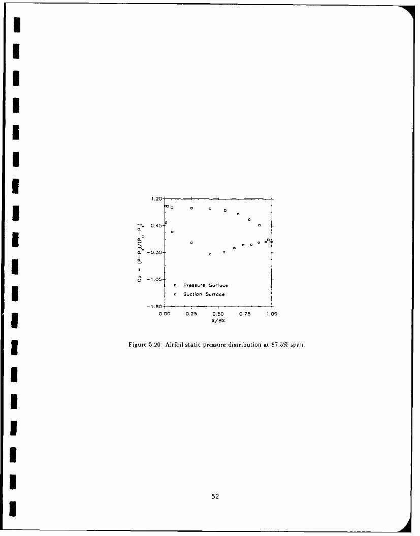
IIIIIII

1.20II 10 lCI a 3 000

0.45-o.

0_ oo

0 0

CL -0.30- 0 0

I I

o - 1.05-0 Pressure Surfoce

0 Suction Surface

-1.80 ' ' " " " ;3 0.00 0.25 0.50 0.75 1.00X/sX

3 Figure 5.20: Airfoil static pressure distribution at 87.5% span.

IIIII

52I

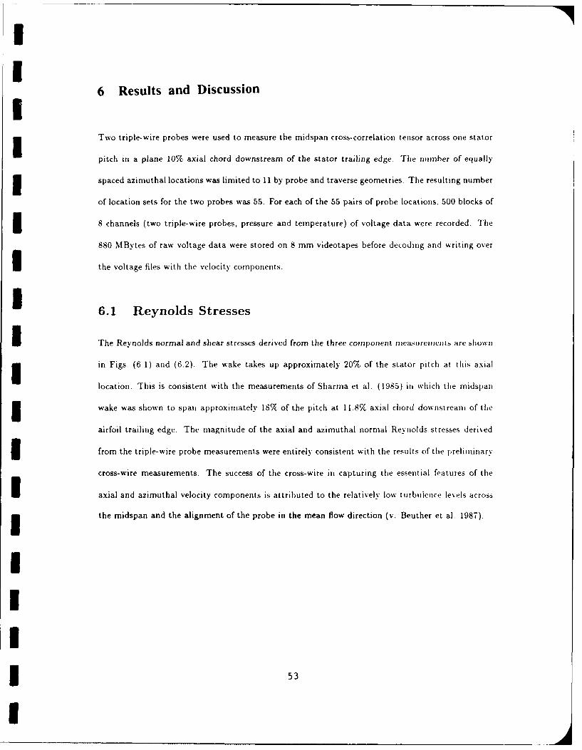
III

6 Results and DiscussionUTwo triple-wire probes were used to measure the midspan cross-correlation tensor across one stator

pitch in a plane 10% axial chord downstream of the stator trailing edge. The number of equally

3 spaced azimuthal locations was limited to 11 by probe and traverse geometries. The resulting number

of location sets for the two probes was 55. For each of the 55 pairs of probe locations, 500 blocks of

8 channels (two triple-wire probes, pressure and temperature) of voltage data were recorded. The

880 MBytes of raw voltage data were stored on 8 mm videotapes before decoding and writing over

I the voltage files with the velocity components.

3 6.1 Reynolds Stresses

I The Reynolds normal and shear stresses derived from the three component mea-surements are shown

3 in Figs. (6 1) and (6.2). The wake takes up approximately 20% of the stator pitch at this axial

location. This is consistent with the measurements of Sharma et al. (1985) in which tile inidspan

3wake was shown to span approximately 18% of the pitch at 11.8% axial chord downstream of the

airfoil trailing edge. The magnitude of the axial and azimuthal normal Reynolds stresses derived

3 from the triple-wire probe measurements were entirely consistent with the results of the preliminar%

cross-wire measurements. The success of the cross-wire in capturing the essential features of the

axial and azimuthal velocity components is attributed to the relatively low turbulence levels across

the midspan and the alignment of the probe in the mean flow direction (v. Beuther et al. 1987).

III

* 5

I

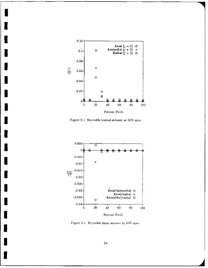
I1

I 0.12"

Axial ( = 1) 0

0.1- 0 Azimuthal (j = 2) +Radial (j = 3) o

0.08-

C17 U 0.06-

* 0.04-

I 0.02- 0

30 20 40 60 80 100

Percent Pitch

3 Figure 6.1: Reynolds normal stresses at 50% span.

I0.005 0

-0.005-

-0.01- +

-0.015-

S-0.02--0.025-

-0.03- Axial/azimuthal 0Axial/radial +

-0.035- Azimuthal/radial 0

-0.0420 40 60 80 100

3 Percent Pitch

Figure 6.2. Reynolds shear stresses at 50'7( span.

I54

I

I!

6.2 Proper Orthogonal Decomposition

The Proper Orthogonal Decomposition was first applied to the entire set of 1089 cross-spectral

3 estimates for the entire stator pitch midspan measurement set. Since there is a large difference in

scales between the wake and outer flow regions, the POD was also applied to those two subdomains.

When the POD is applied in inhomogeneous directions after harmonic decomposition in the

homogeneous directions, the spectral tensor can be expressed as a bilinear combination of the eigen-

I modes (Herzog, 1986). The reconstruction of the cross-spectral tensor can be expressed as

3 "S , k (0. O.) k ) (6.1)n=1

I Equation (6.1) is analogous to the representation of the cross-correlation tensor shown in Eq. (2.9).

The results of this reconstruction for i = j yields the power spectral density (PSD) of the each

3 velocity component. Thus, to evaluate tile adequacy of the eigenmodes to represent the flowfield,

the measured power spectral densities can be compared to reconstructions based on the eigenniodes

I and eigenvalues. In the following sections, the PSD data are compared to reconstruct ions using the

first five (dominant) POD modes.

3 6.2.1 Full Domain: 0-100% Pitch

The eigenspectra of the five dominant modes extracted by the POD are shown in Fig (6.3). The

I eigenspectra represent the energy content of each of the eigenniodes. Figure (6.3) resembles the

eigenvalue plots of Chambers et al. (1988). In that work, the Karhunen-Loeve expansion was

applied to the solution of a randomly forced, one dimensional Burgers' equation with boundary

3 conditions conducive to the development of thin boundary layers at the edges of the computational

domain. The spectrum of the interior region of their calculation domain has the same character

3 including the leveling off at high frequencies ('sequencies' in their terminology). It is suggested

here that the increased energy content of the high frequency eigenspectra is due to the sijhstantial

broadband energy of the wake. As.-is shown in Section (6.2.2), the high frequel cy fiat teling is

3 eliminated when the viscous wake region is not included in tile POD donaini lh, first mIde was

55I

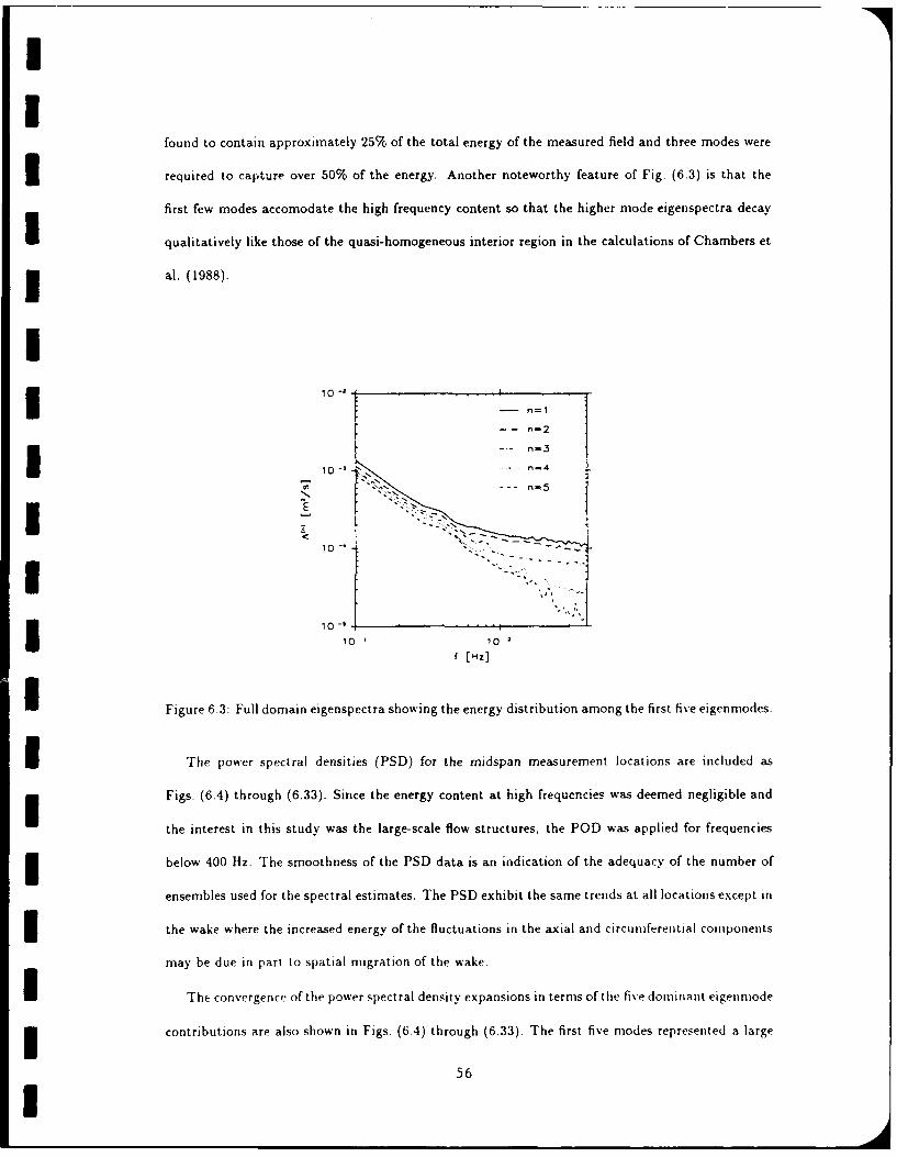
IU

found to contain approximately 25% of the total energy of the measured field and three modes were

3 required to capture over 50% of the energy. Another noteworthy feature of Fig. (6.3) is that the

first few modes accomodate the high frequency content so that the higher mode eigenspectra decay

qualitatively like those of the quasi-homogeneous interior region in the calculations of Chambers et

3 al. (1988).

II 10 4- n-4

--- n=2i --- n-35 o-*f.'.. .. ....

IE10-Il

I 10 -s

10' 10*f [Hz]

I Figure 6.3: Full domain eigenspectra showing the energy distribution among the first five eigenmodes.

I The power spectral densities (PSD) for the midspan measurement locations are included as

Figs. (6.4) through (6.33). Since the energy content at high frequencies was deemed negligible and

the interest in this study was the large-scale flow structures, the POD was applied for frequencies

below 400 Hz. The smoothness of the PSD data is an indication of the adequacy of the number of

ensembles used for the spectral estimates. The PSD exhibit the same trends at all locations except in

the wake where the increased energy of the fluctuations in the axial and circumferential components

may be due in part to spatial migration of the wake.

I The convergence of the power spectral density expansions in terms of the five dominant eigenmode

contributions are also shown in Figs. (6.4) through (6.33). The first five modes represented a large

56I

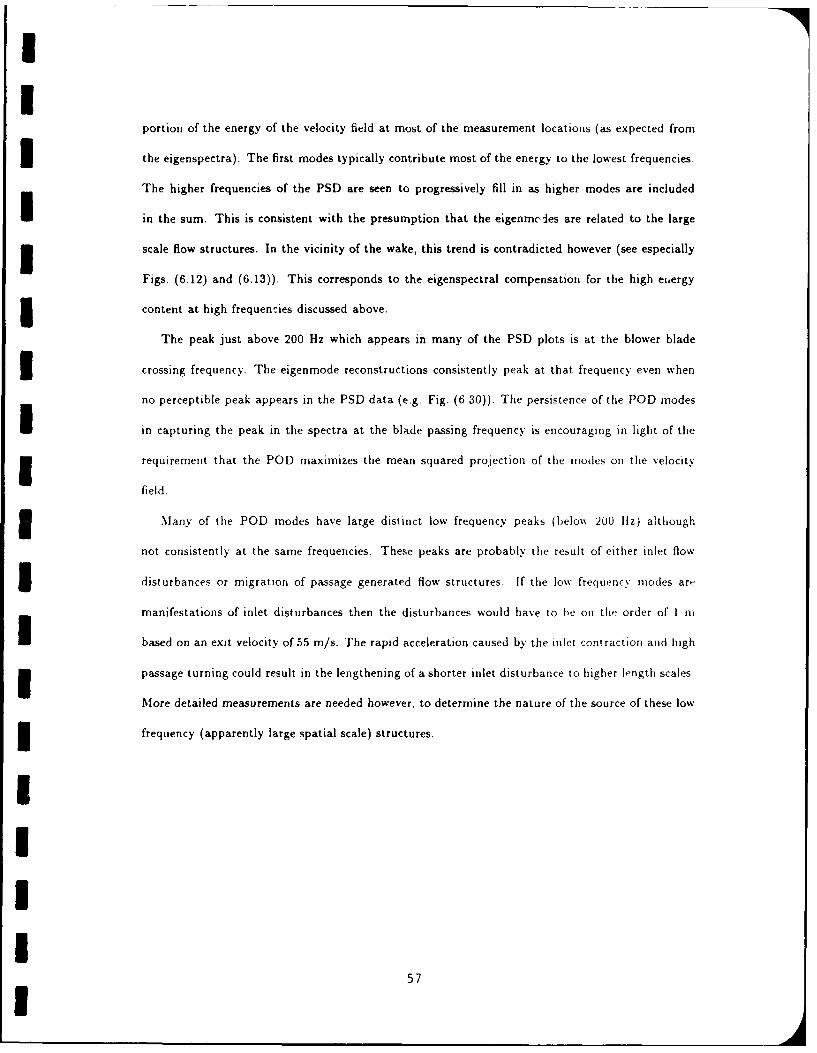
II

portion of the energy of the velocity field at most of the measurement locations (as expected from

the eigenspectra). The first modes typically contribute most of the energy to the lowest frequencies.

The higher frequencies of the PSD are seen to progressively fill in as higher modes are included

in the sum. This is consistent with the presumption that the eigenmcies are related to the large

3 scale flow structures. In the vicinity of the wake, this trend is contradicted however (see especially

Figs. (6.12) and (6.13)). This corresponds to the eigenspectral compensation for the high euergy

content at high frequencies discussed above.

The peak just above 200 Hz which appears in many of the PSD plots is at the blower blade

3 crossing frequency. The eigenmode reconstructions consistently peak at that frequency even when

no perceptible peak appears in the PSD data (e.g. Fig. (6.30)). The persistence of the POD modes

in capturing the peak in the spectra at the blade passing frequency is encouraging in light of the

3 requirement that the POD maximizes the mean squared projection of the modes on tie velocity

field.

3 Many of the POD modes have large distinct low frequency peaks (below 200 liz) although

not consistently at the same frequencies. These peaks are probably the result of either inlet flow

3 disturbances or migration of passage generated flow structures. If the low frequency modes are

manifestations of inlet disturbances then the disturbances would have to be on the order of 1 II

based on an exit velocity of 55 m/s. The rapid acceleration caused by the inlet contraction and high

I passage turning could result in the lengthening of a shorter inlet disturbance to higher length scales.

More detailed measurements are needed however, to determine the nature of the source of these low

3 frequency (apparently large spatial scale) structures.

IIII

57I

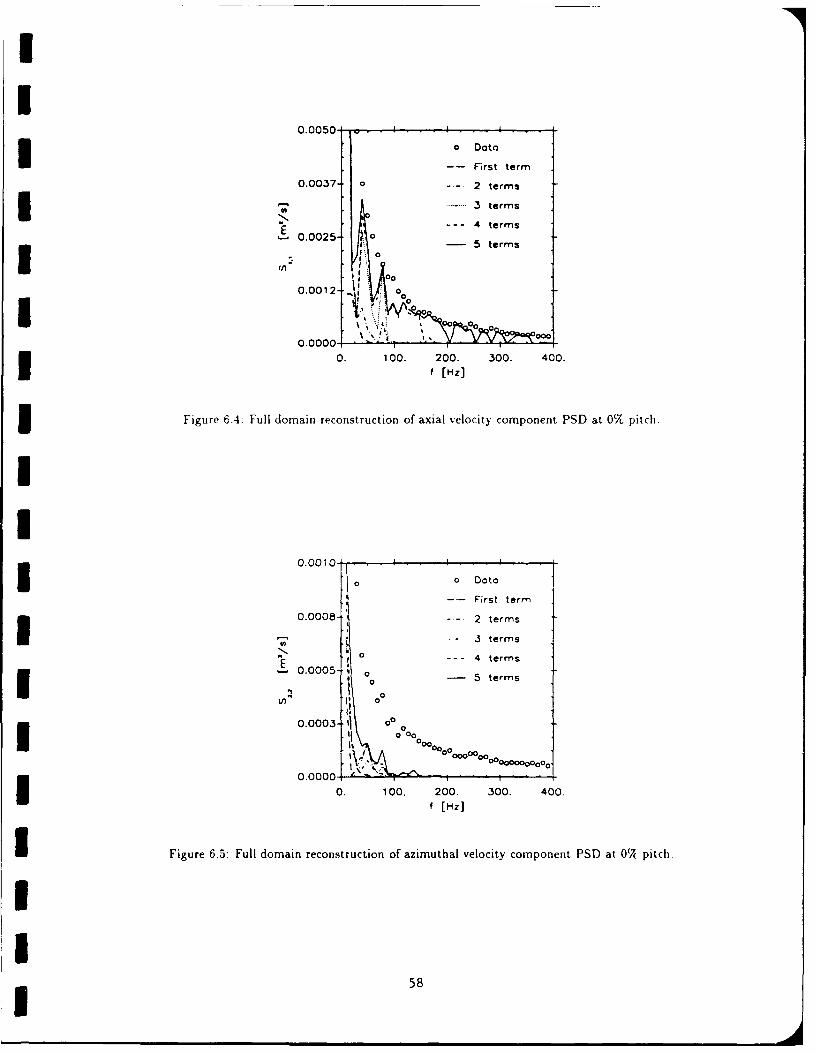
II

0.00 5 0-o I I i

-- First term

0.0037- o 2 terms

3 terms

-- - 4 terms

O - 0

00

0.0012 -i

0.0000 "

0. 100. 200. 300. 400.

f [Hz]

5 Figure 6.4: Full domain reconstruction of axial velocity component PSD at 0% pitch.

II 0.0010 0 2 te

-- First term

0.0008--- 2 terms

.3 terms0-- - 4 terms

0 o.oo5 terms

0 00

00 00 0 000000

0.0000, 00.00O. 100. 200. 300. 400.

f [Hz]

I Figure 6.5: Full domain reconstruction of azimuthal velocity component PSD at 0'( pitch.

5

58

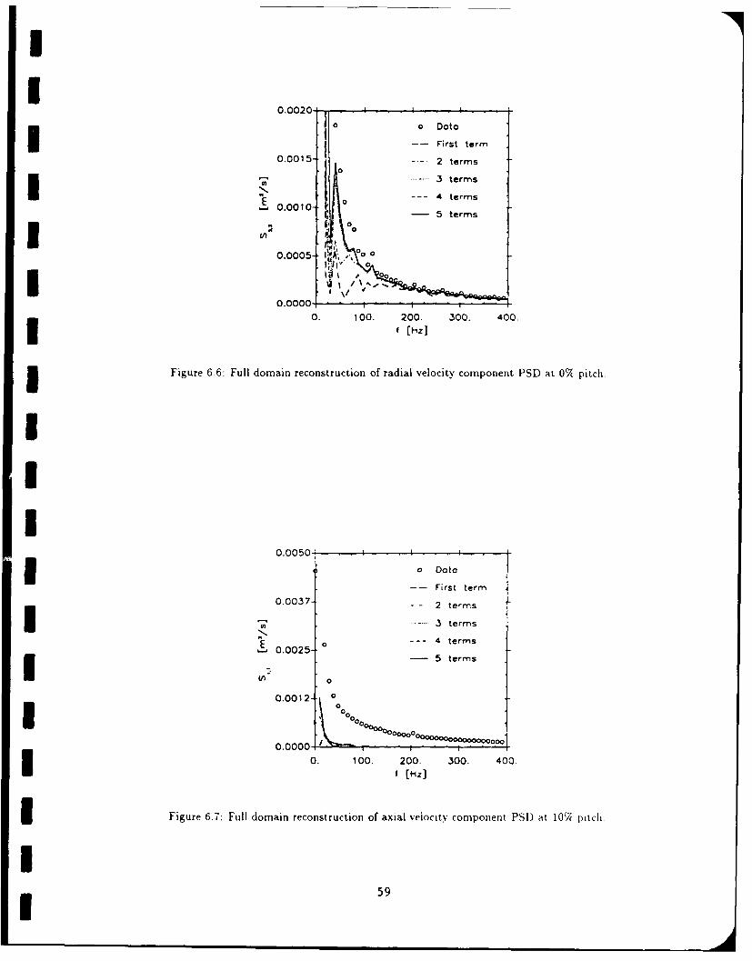
0.0020- I

0 0 Data

0.0015- First term

0.001 - -2 terms-3- terms

temE 3 terms

0.0010 -5 terms

0.0005 I.t

000. 100. 200. 300. 40

5 Figure 6.6: Full domain reconstruction of radial velocity component PSD at 0%c pitch.

0.0050- I

Z 0 Data-- First term

0.0037-- 2 terms

- - 3 terms

E - - -4 termsE0.0025-

em

0.0012- 0

0

0.0000-0. 100. 200. 300. 400.

f(HZ]

3 Figure 6.7: Full domain reconstruction of axial velocity component PSI) at 1Oi pitch

I 59

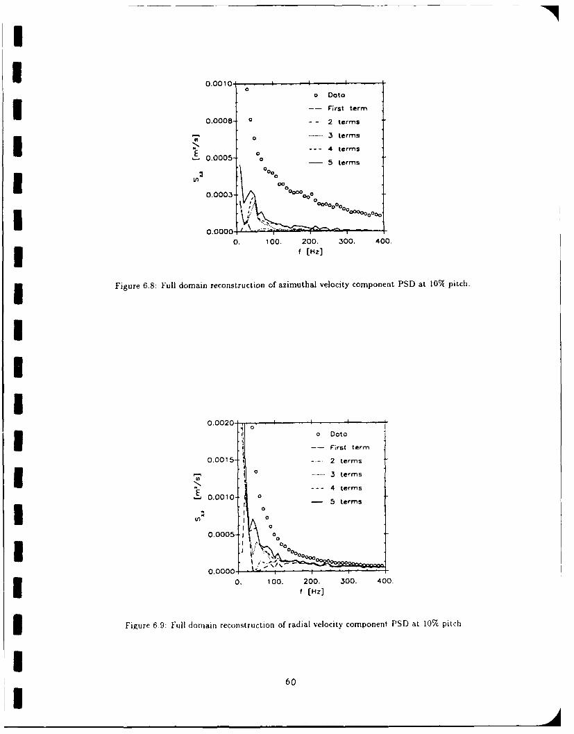
0.001I

1 Data

-- First term

0.0008 0 2 terms

0 . 3 terms

-- - 4 terms"E 00 0

0.0005- '0 5 terms

000

0.0003- 0 0000 00 00000000 0.

0.0000 a

0. 100. 200. 300. 400.f [Hz]

Figure 6.8: Full domain reconstruction of azimuthal velocity component PSD at 10% pitch.

U

I0.0020 - . .

o Data

-- First term

0.0015- 2 terms

S......3 termsI--- 4 termsE0.0010. 0 5 terms

I0.0005- 1 0

O.O 00 .L-- . ; • • -0•00--00,0.0005

0. 100. 200. 300. 400.

f [Hz]

Figure 6.9: Full domain reconstruction of radial velocity component PSD at 10% pitch.

60I

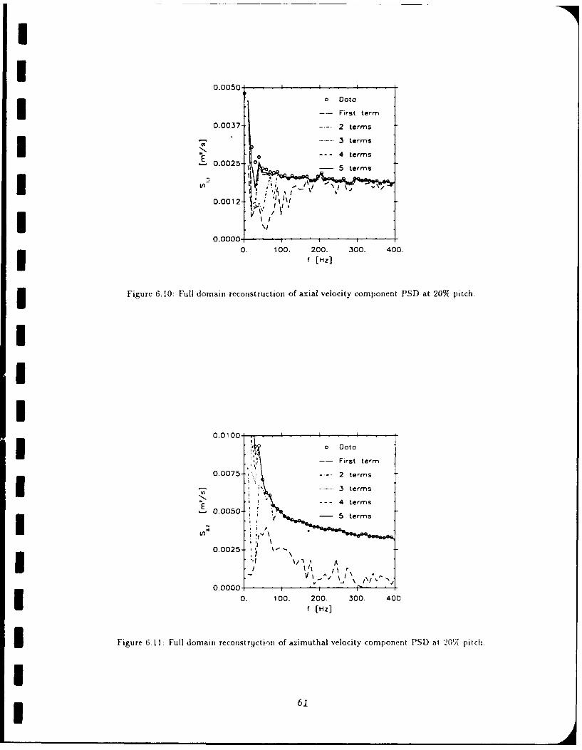
I

0.0050 - I i

o Doto

-- First term

0.0037- -.- 2 terms

3 terms@1IN --- 4 terms

00025- '1° _ 0- 5 terms

0.0012- 1i;I I

0.0000.

0. 100. 200. 300. 400.f [Hz]

Figure 6.10: Full domain reconstruction of axial velocity component PSD at 20% pitch.

iII

0.0100'

o Doto

-- First term

0.0075- 2 terms

3 termsr, i "L --- 4 terms •

"E0.0050- 5 terms

0.0000 1-0. 100. 200. 300, 400.

f [Hz]

I Figure 6.11: Full domain reconstryction of azimuthal velocity component PSD at 20'( pitch.

I

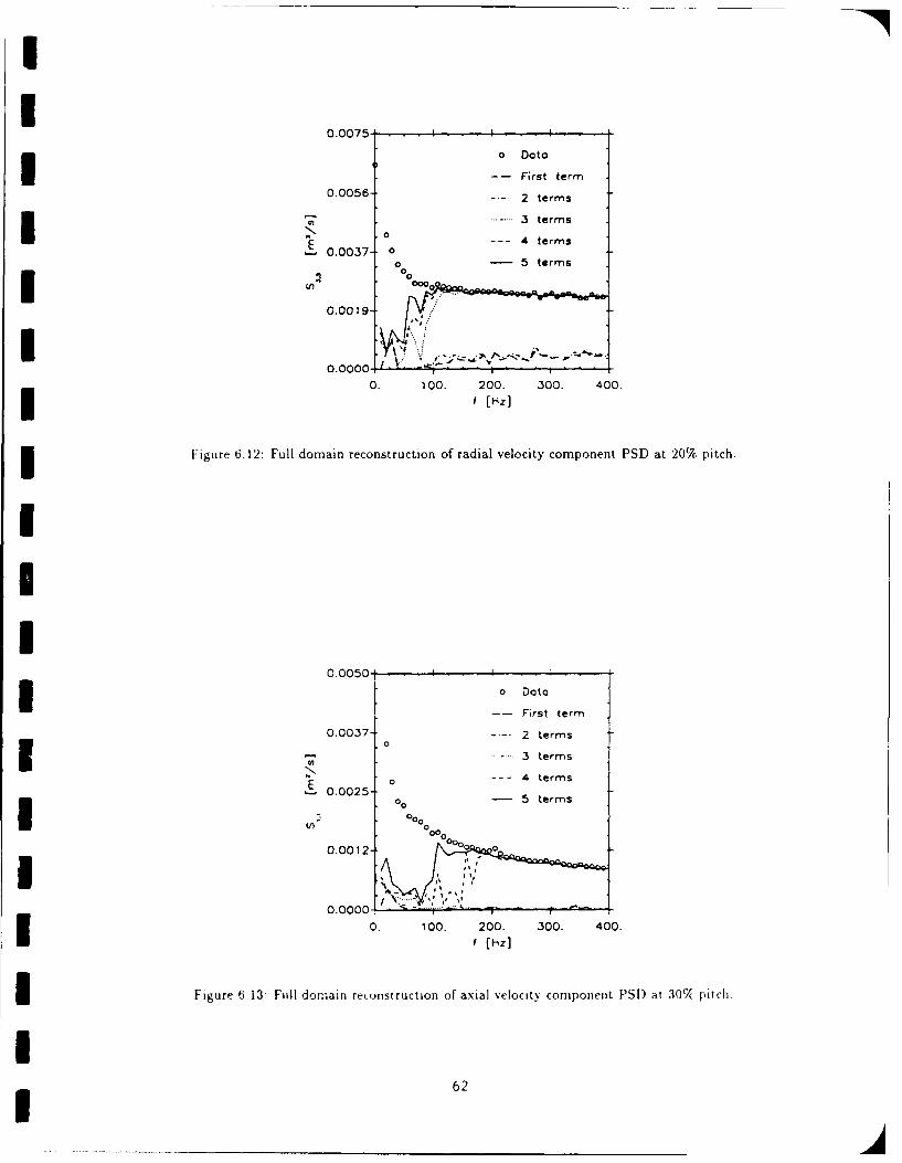
0.0075- I I

0 Data

-- First term

0.0056-- - 2 terms

3 terms

0 -- 4 te m

E0.00300/ '--

0. 100. 200. 300 400.f [Hz]

Figure 6.12: Full domain reconstruction of radial velocity component PSD at 20%, pitch.

0.0050

* Data

-- First term

0.0037-- 2 terms0

- - 3 terms

E0.0025- 00 - terms

0.0000 ,0. 100. 200. 300. 400.

f [Hz]

I Figure 6.13 FiilI domnain re~ulistruction of axial velocity component PSO at 30% pitch,

62

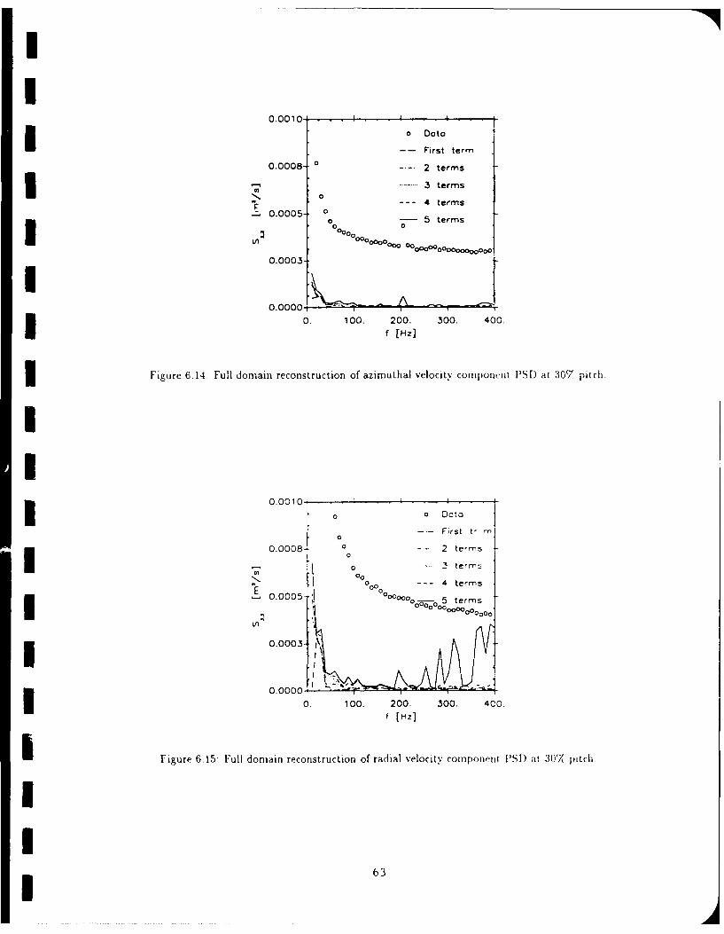
I

0.0010 I I .

0 Dato

-- First term

0.0008- 0 2 terms

I..3 terms

S--4 terms0.0005- 05 terms

Ln 3 0 000 0000 00 000000"000"0.

0.0003-

0.0000,0 0. 100. 200. 300. 400.

f [Hz]

3Figure 6.14: Full domain reconstruction of azimuthal velocity componcnt PSD at 307 pitch.

I

i ~ ~~~~~~~0.00101 -0 o D0ta

0 --- First t- ry

00.0008- 0- 2 terms

,- o .... 3 term :,

000 --- 4 terms

E 00.00 5e0.0005 0 5 terms

000000000000

~~0.0003- (

I0.00001-7-

0. 100. 200. 300. 4C0.

f [Hz]

i Figure 6.15: Full domain reconstruction of radial velocity component PSD at 30'7 pitch

II 63

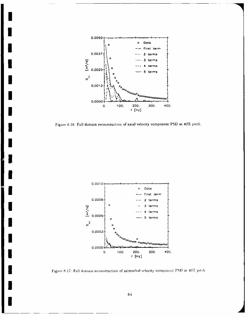
I

0.0050 .

0 Doto*0-- First term

0.0037- --. 2 terms0 3 terms

S

E --- 4 terms0.0025"- 5 terms

Si 0

Lfl ?' 0o0

0.0012 k. 0' i -0

0.0000 0

0. 100. 200. 300. 400.

f [Hz]

Figure 6.16: Full domain reconstruction of axial velocity component PSD at 40% pitch.

I

I0.0010 i

3 o Data

-- First term

0.0008 .. . 2 term s

0 3 terms

--- 4 termsE-.0.0005- 5 termsI°

00

0.0003- 000

00 000 / oooo0o0ooooooo00

o0o0000 o

0. 100. 200. 300. 400.f [Hz]

Figure 6 17: Full domain reconstruction of azimuthal velocity component PSD at 40V pitch

164I

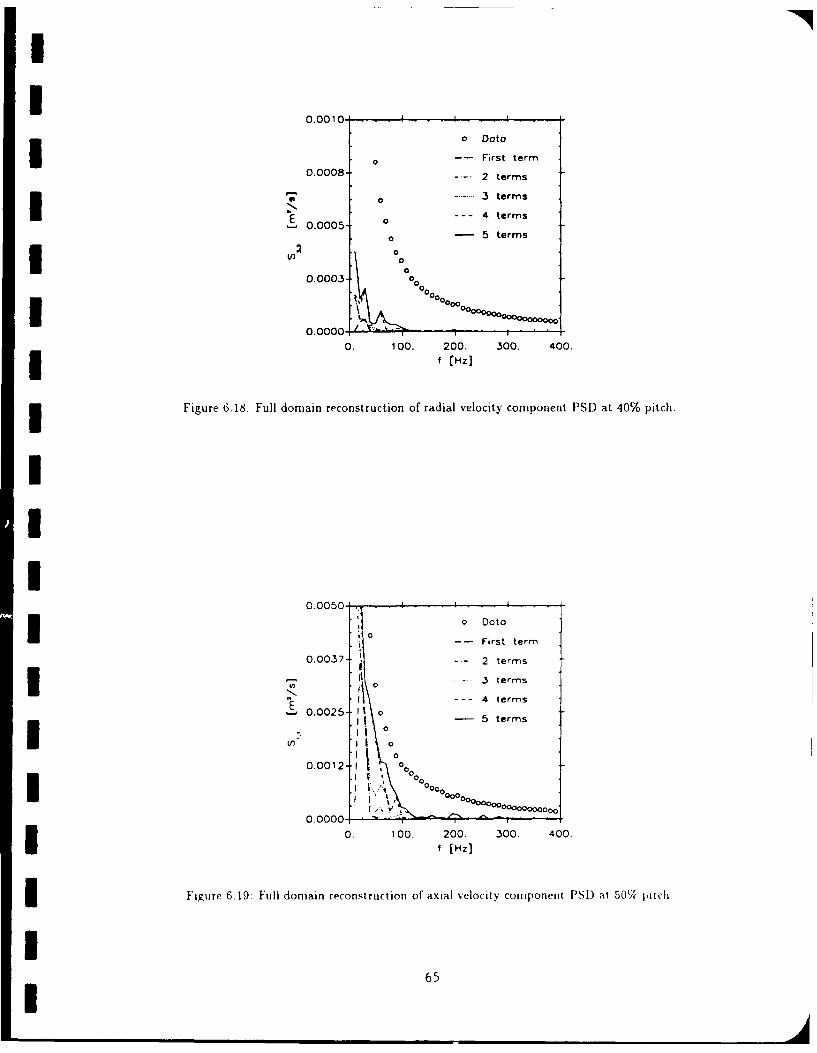
0.0010 I

0 Data1 0-- First term

0.0008-- 2 terms

0... -3terms

-- 4 terms

0

000 0.0005

0.00 1 0 ,000. 100 20 30. 4.

f [Hz]

U Figure 6.18: Full domain reconstruction of radial velocity component PSD at 40% pitch.

0.0050-0 Dcta

.0 -- First termU 0.0037-- 2 terms

-3 termsI 0- Ii - -- 4 terms

L 0.0025- o 5 terms

ii0U1 0I 00.00121 0)

**.*1 0000I ,' j..0. 0000 00000000000000000

0.0000-0. 10. 200. 300. 400.If [Hz]

Figure 6.19: Full domain reconstruction of axial velocity component PSI) at 50'7 pitch,

65

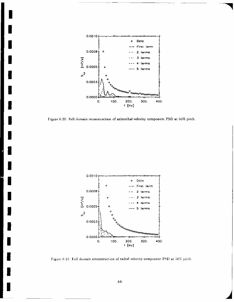
I0.0010 .

0 Doto

--- First term

0.0008- 0 2 terms

........ 3 terms

-- - 4 terms0.0005- 5 terms

0.0003- 00I 00000000000000000000000

0.0000- 1 . 1

0. 100. 200. 300. 400.If [Hz]

Figure 6.20: Full domain reconstruction of azimuthal velocity component PSD at 50% pitch.

I

I0.0010 . ,

0 Dato

0 -- First term

0.0008- -- 2 terms

71-0 3 termsS0.0 0 0 5 .te rm s

.

--- 4 terms

0.0005-- 5 terms

0I0.0003- 00

•

000

0. 100. 200. 300. 400.

Hz]

IFigure 6 21 Full domain reconstruction of radial velocity component PSI) at .507( pitch

66

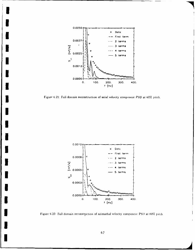
I

0.0050 "

0 Doto33 -- First term

0.0037 i. 2 terms

3 terms

.002 0 --- 4 terms

0.0 -55 termsI

ID

0.0012 0

0.0008- - 2tem

S0000000000000..01..

0.0000- o

0.000 100. 200. 300. 400.

3 Figure 6.22: Full domain reconstruction of axial velocity component PSD at 60'7(, pitch.

0. 00 10

0 Data-- First term

II 0.000 - o 2 terms

0 00 004

0 0 O O O o o O0

0.00 . t - ,. 100. 200. 300. 400.

f [Hz]

3 Figure 6.23: Full domain reconstruction of azimuthal velocity component PSD at 607( pitch

I67U

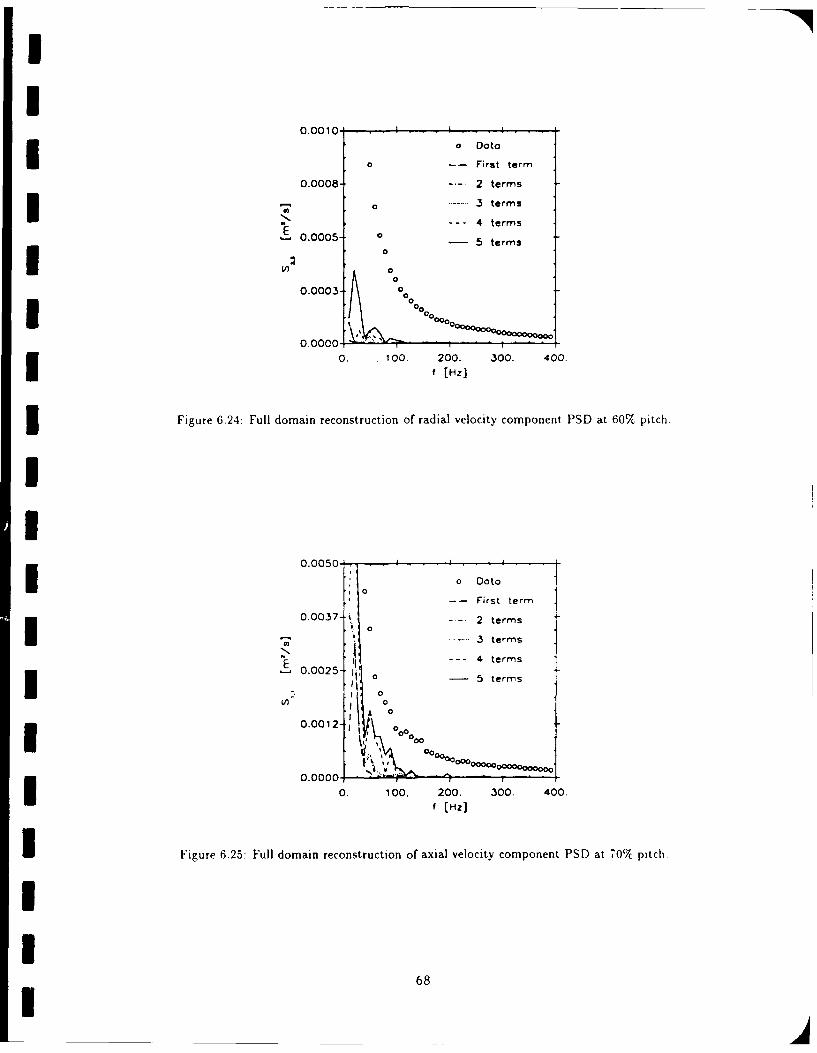
I'U

0.00100 Doto

0 -- First term

0.0008- 2 terms

.- 0 3 terms

4 terms

__ 0.0005- 0 5 terms0

I o t00

0.0003- 000

0000

0.0000 - '0. 100. 200. 300. 400.

f [Hz]

3 Figure 6.24: Full domain reconstruction of radial velocity component PSD at 607, pitch.

I

0.0050 . . . . . . . .

o Doto0 -- First term

i 0.0037- 0 2 terms

I3 terms

4terms0.0025- o - 5 terms

S terms

I 0.0012- 000 0 0

• ! '.0 0 0 0 0000 0 0 ̂ -

i .0000+ 000 ,

0. 100. 200. 300. 400.f [Hz]

I Figure 6.25: Full domain reconstruction of axial velocity component PSD at 707c pitch.

II

68I

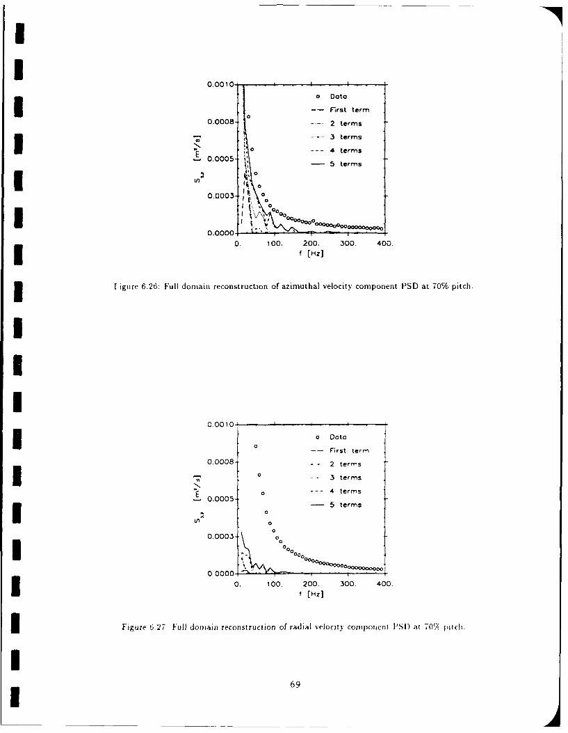
I

0.0010- I I

o Data

.--- First term0.0008-1 ] .. 2 terms

-...3 terms

S0.0005 04 terms.005 i,0

-- 5 terms

0

0.0003

~00

I m

I oo000

0.0000-0. 100. 200. 300. 400.

f [Hz]

3 I igure 6.26: Full domain reconstruction of azimuthal velocity component PSD at 70% pitch.

III

0 .0 0 1 0D a t aI0 Data-- First term

0.0008- -- 2 terms

.0 3 term s

0 0 -- - 4 termsI .00 0 5 terms

~00.0003- 0 -~o

0 0000

- %~~~00ooo00 ooo0o0

0. 100. 200. 300. 400,

f (Hz]

I Figure 6.27 Full domain reconstruction of radial velocity component PSD at 70'7 pitch.

II 69

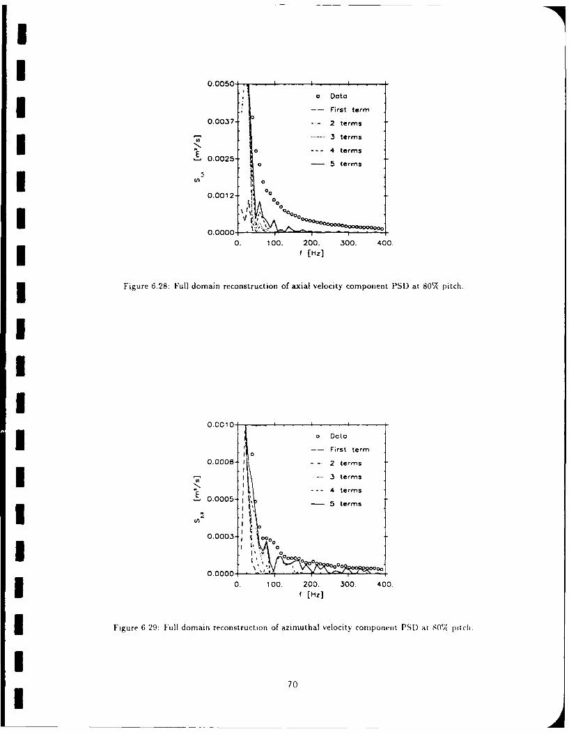
I

0.0050 - I

a Data

-- First term

0.0037- .. 2 terms

3 terms

0.0 0 --- 4 terms0 =0 5 terms

W 00.0012- 00

00.0000,

0. 100. 200. 300. 400.

f [Hz]

Figure 6.28: Full domain reconstruction of axial velocity component PSD at 80%A pitch.

III

0.0010-

0 Dota

-- First term

0.0008- t 2 terms

3 terms

-4 terms0.0005- 5 termsI- 5- terms! I

0-0003 ~ 00 4000

0 0

0.00O. 100. 200. 300. 400.

f [Hz]

~Figure 6.29: Full domain reconstruction of azimuthal velocity component PSD at S0V( pitch

70

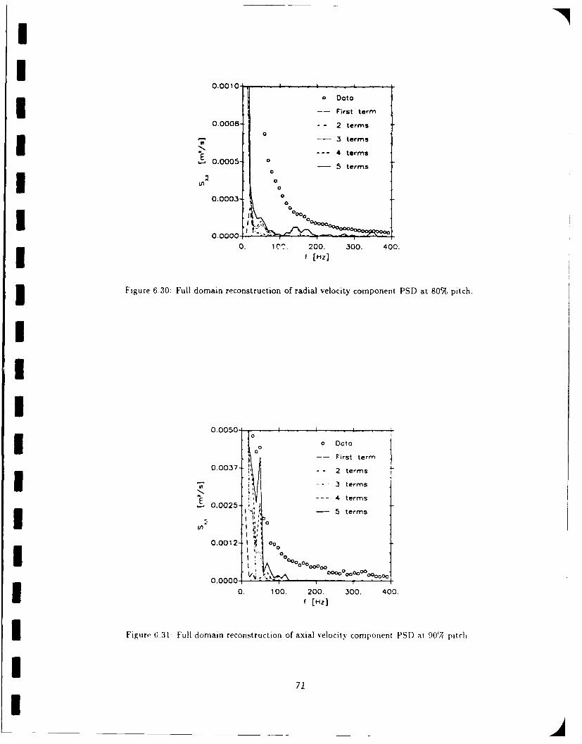
I -

0.0010 I I

I o Data

-- First term

0.0008- 2 termsS3 terms

> 4 terms0.0005-

- 5 terms

0

0.0003- 00II

0.0000 -.

0. 1Cr. 200. 300. 400.

f [Hz]

3 Figure 6.30: Full domain reconstruction of radial velocity component PSD at 80% pitch.

I,I

I0.0050- I . I

0So0 Dato

0

: .:: -- First term

- termsE i.~t - 4 terms

0,0025- .I5 terms

0,0012- 1 0

S(l %0000 o00

0. 100. 200. 300. 400.f [Hz]

3 Figure 6.31. Full domain reconstruction of axial velocity component PSD at 90'7 pitch.

I72

I

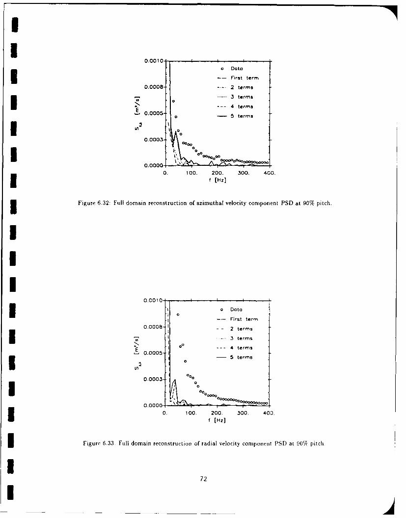
I

0.0010 I I ia Data

-- First term

0.0008- . . 2 terms

1 3 terms

-- - 4 terms0.0005.

E0.00053 0 - 5 terms

0.0003 00000

0. 100. 200. 300. 400.

I Figure 6.32: Full domain reconstruction of azimuthal velocity component PSD at 90% pitch.

II

0 .0 0 10 t .. . .

0 DataI 0-- First term

0.0008 " o 2 terms

.. 3 terms

I 0- 4 termsE 0.0005- 1-5 terms

o 0oo , o0.0003- 00000

0 .0 0 0 00 0 0 0

0. 100. 200. 300. 400.f [Hz]

Figure 6.33: Full domain reconstruction of radial velocity component PSD at 90'/( pitch.

I772

If

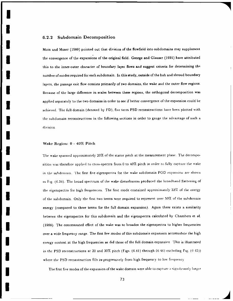
Iii

6.2.2 Subdomain Decomposition

Moin and Moser (1989) pointed out that division of the flowfield into subdomains may supplement

the convergence of the expansions of the original field. George and Glauser (1991) have attributed

this to the inner-outer character of boundary layer flows and suggest criteria for determining the

number of modes required for each subdomain. In this study, outside of the hub and shroud boundary

layers, the passage exit flow consists primarily of two domains, the wake and the outer flow regions.

I Because of the large difference in scales between these regions, the orthogonal decomposition was

3 applied separately to the two domains in order to see if better convergence of the expansion could be

achieved. The full domain (denoted by FD), five term PSD reconstructions have been plotted with

the subdomain reconstructions in the following sections in order to gauge the advantage of such a

division.IWake Region: 0 - 40% Pitch

The wake spanned approximately 207 of the stator pitch at the measurement plane. The decompo-

sition was therefore applied to cross-spectra from 0 to 40% pitch in order to fully capture the wake

in the subdomain. The first five eigenspectra for the wake subdomain POD expansion are shown

in Fig. (6.34). The broad spectrum of the wake disturbances produced the broadband flattening of

the eigenspectra for high frequencies. The first mode contained approximately 33% of the energy

I of the subdomain. Only the first two terms were required to represent over 507 of the subdomain

I energy (compared to three terms for the full domain expansion). Again there exists a similarity

between the eigenspectra for this subdomain and the eigenspectra calculated by Chambers et al.

3 (1988). The concentrated effect of the wake was to broaden the eigenspectra to higher frequencies

over a wide frequency range. The first few modes of this subdomain expansion accomodate the high

3 energy content at the high frequencies as did those of the full domain expansion. This is illustrated

in the PSD reconstructions at 20 and 30'/ pitch (Figs. (6.41) through (6.46) excluding Fig. (6.45))

I where the PSD reconstruction fills in' progressively from high frequency to low frequency

3 The first five modes of the expansion of the wake domain were able tocapure a significantly larger

73I

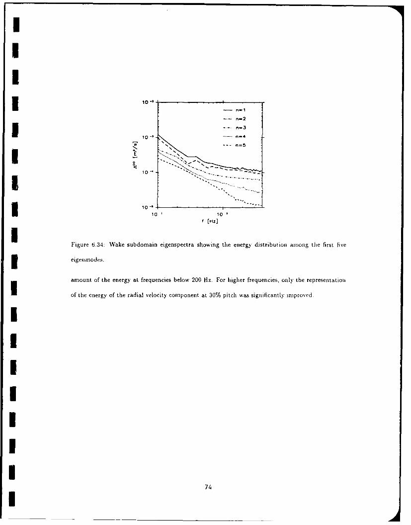
U10-2- In-2

n-3

I 10-3' n. n-4

N -- - n=5

10 -* ------__ _ __ _ __ _ __ _ _110' 10 2f(Hz]

I Figure 6.34: Wake subdomain elgenspectra showing the energy distribution among the first five

3 eigenmodes.

amount of the energy at frequencies below 200 Hz. For higher frequencies, only the representation

I of the energy of the radial velocity component at 30% pitch was significantly improved.

I7

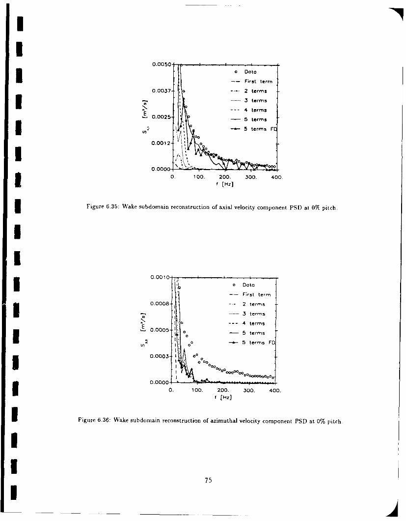
0.0050 -

0DataI a First term

0.0037- 0 - 2 terms

__

terms

---

4terms

0.002 - 5terms

00 -~-5 termsF0.00125 50em

'4 000

0.0000 000-I0. 10 0. 200. 300. 400f[Hz]

Figure 6.35: Wvake subdomain reconstruction of axial velocity component PSD at 0% pitch.

0.00 10-* a Data

-- First term

0.0008-- 2 terms

3 terms

0 00--- terms

E .005 0 -5 terms

00*' 5 terms FD

I0.0 0 0 3 - 1 000 , 00

0.0 00 0 000o0

0. 100. 200. 300. 400.

I Figure 6.36: Wake subdomain reconstruction of azimuthal velocity component PSD at 0% pitch.

7 5

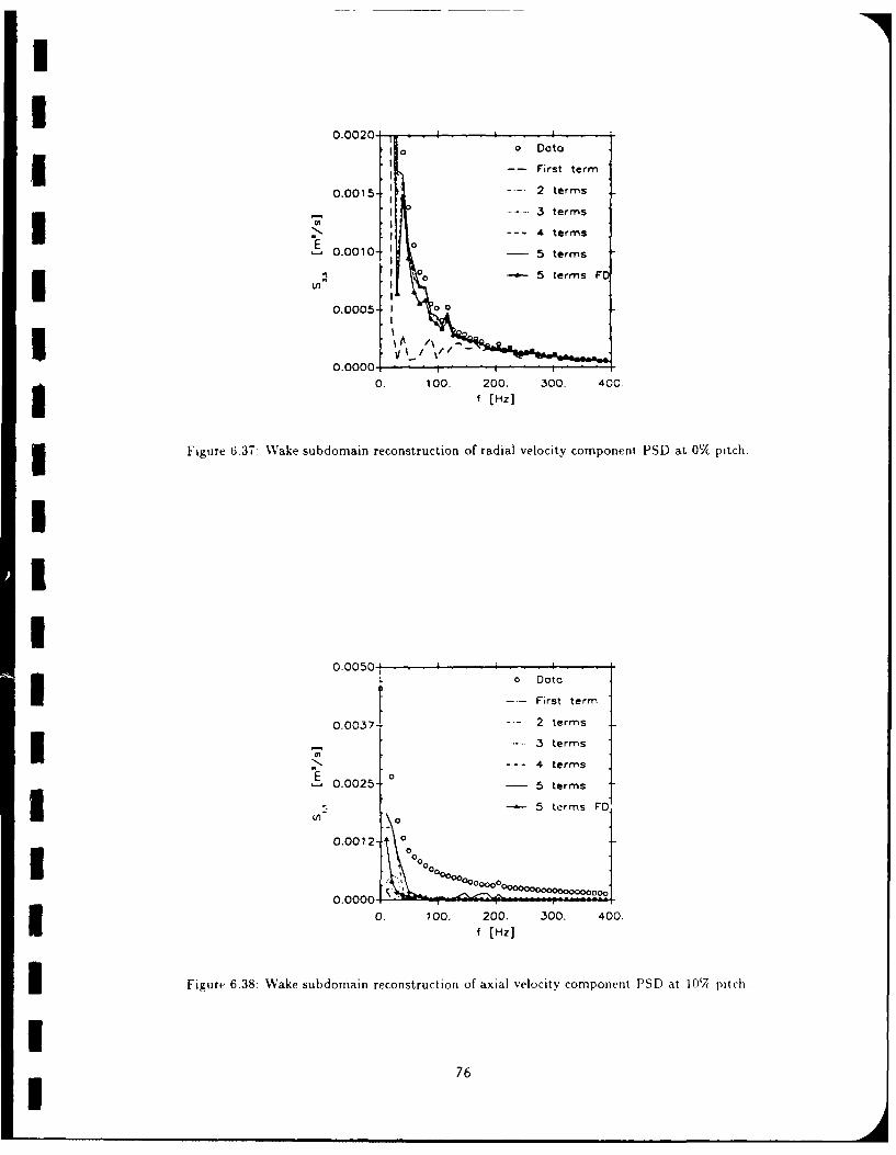
I

0.0020-- rI

l o 0 D a ta

-- First te rm

0.0015- - 2 terms

--- 3 terms

I -- 44terms

- 0.0010-

5- terms" 5 terms

1I 0 5 terms FPI/

0. 0005- 1 o

II/ F0.0000 -

0. 100. 200. 300. 400.

[Hz]

3 Figure 6.37: Wake subdomain reconstruction of radial velocity component PSD at 0% pitch.

[

I0.0050Dat

a Data

-- First term

0.0037- - 2 terms

-3 terms

--- 4 termsE o0.0025- - 5 terms

- -- 5 terms FO

0.0012- 0

00 0o

0.0000 "

0. 100, 200. 300. 400.

f [Hz]

Figure 6.38: Wake subdomain reconstruction of axial velocity component PSD at 10'7 pitch,

I76I

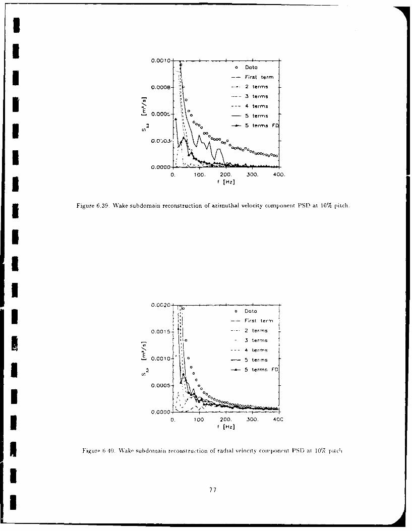
0.0010 ----.- j

0 Data

-- First term

I 0.0008-. 2 terms

0 3 terms

E - - -4 terms

0 .00i 5tem

0. 100. 200 00. 40

3 Figure 6.39. Wake subdomain reconstruction of azimuthal velocity component PSD at 10%/C pitch.

0 Doto

-- Frst term

0.00154 2 Ijfj rms1 -s--- 5 terms F

0.0010 5 em

f iur 64 W Ir 0 5 te00s FD0. 4 C s~ a 10 1

sibdrninreon! uc in f adalveoct

0 .0 5 -0770I0

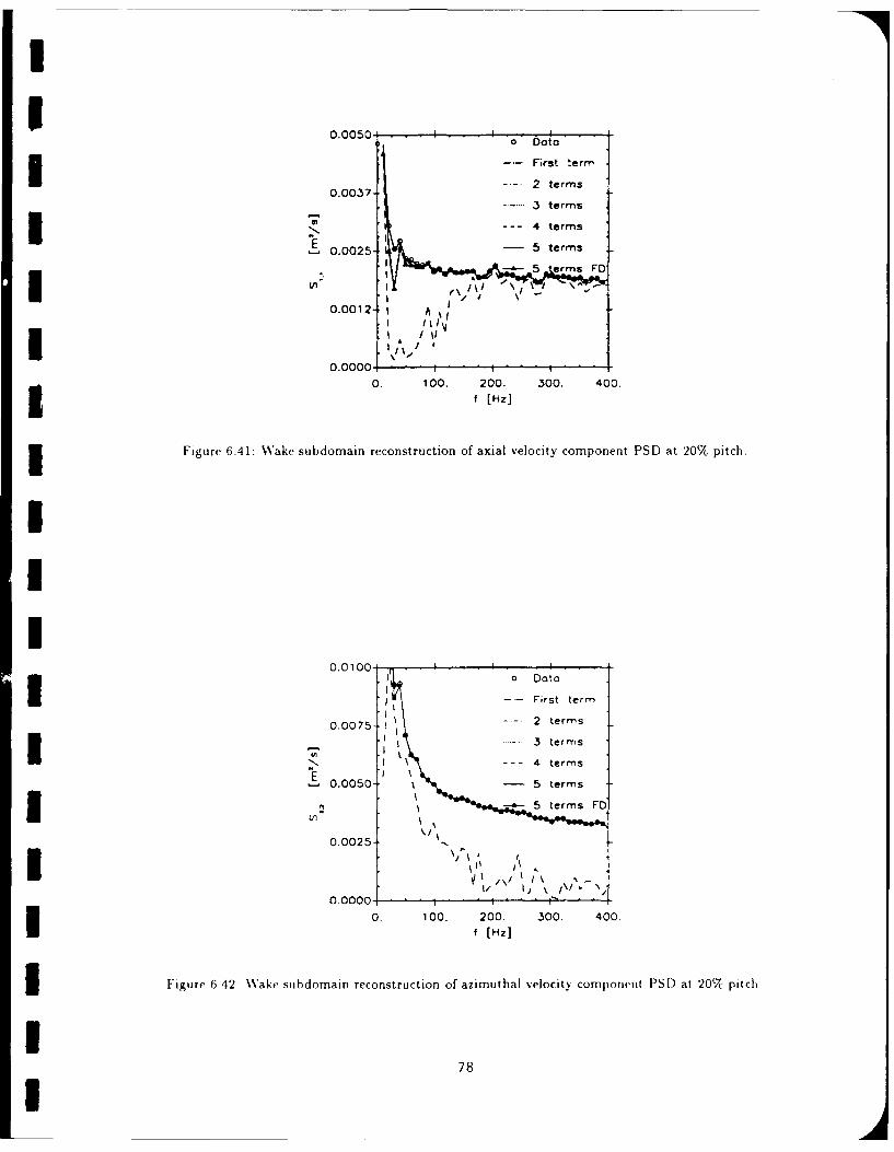
10.0050- 0 Data

-- First lerry'

- 2 terms0.0037 3tem

N -- 34terms

E0.0025- em

* - IY

0 . 1 0 . 0 0 3 L0 4 0 0

Figure 6.41: Wake subdomain reconstruction of axial velocity component PSD at 20%/( pitch.

0.0 100-aDt

-First term

0.075 2terms

I3 te rms

0.0000- 0.~ ~ ~~ 10. 20. 30. 40[Hter]

3 Figure 6.42 Wak subdomaip reconsruction of azimutaoctcmpetPS)a20pihI em,n 4 te78EI

1 0.00750 Data

-- First term

0.0056- 2 terms

- 3 terms

0.0000 . 200 300. 400

0.0050 I1

0 DataI-- First term

0.0037- 2 terms

*3 terms

I 4 terms

0.000. 20.100240

f [Hz]

Figure 6.44: Wake subdomnain reconstruction of axial velocity component PSD at 30% Pitch

79

I

0.0010 - o0 Data

-- First term

0.0008- 0 2 terms

o -- 3 terms0 4 terms

E 0.0005- 0 - 5 termsI o00 0

in -'- 5 terms FD

u00000-o.oooo

0.0003-

I ~0.0000Je 1h. ._ , -

0. 100. 200. 300. 400.

f [Hz]

3 Figure 6.45: Wake subdomain reconstruction of azimuthal velocity component PSD at 30% pitch.

0.0015- oo Data

0 -- First term

0.0011 - - 2 terms

S... 3 terms

0 - -- 4 terms- 0.0008- 0o o - 5 terms

0 0o00o,. 5 terms FO

5 0. 100. 200. 300. 400.I (Hz]

IFigure 6.46: Wake subdomain reconstruction of radial velocity component PSD at. 30% pitch.

II

1 80

It

3 ~ ~~0.0050 aDtatr

0 0.0Firs2 trm

--- terms

IE0.0025- 0 -5 terms

0 - 5 terms FO'

0.00 12-~

0.0000-0. 100. 200. 300. 400.3 f [Hz]

3 Figure 6.47: Wake subdomain reconstruction of axial velocity component PSD at 4UtXc pitch.

0O0010 I0 Data

-- First term

0 0008 - 2 terms

0 3 termsI --> 4 terms0.0005 - 5 terms

0

-~-5 terms FOIn 000.0003 - 0 0

0.0000-

0. 100. 200. 300. 400.

f[Hz]

Figure 6.48: Wake subdomain reconstruction of azimuthal velocity component PSD at 407c pitch.

81

II '

II,I'I

0.0010 0 t , a . . .

-- First terma

0.0008 . 2 terms

£~ ~ terms- 4 terms

- 0.0005- - 5 terms

00-o - 5 terms FD

S0.0003- aa0

0.0000 -- 00 0OC 0000 0 000aa

0. 100. 200. 300. 400.f [z]

Figure 6.49: Wake subdomain reconstruction of radial velocity component PSD at 40'7 pitch.

II

III

82U

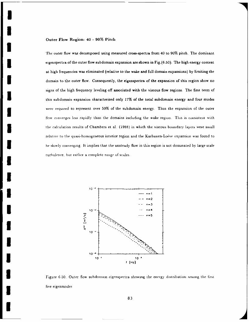
II

Outer Flow Region: 40 - 90% PitchIThe outer flow was decomposed using measured cross-spectra from 40 to 90% pitch. The dominant

eigenspectra of the outer flow subdomain expansion are shown in Fig.(6.50). The high energy content

at high frequencies was eliminated (relative to the wake and full domain expansions) by limiting the

3 domain to the outer flow. Consequently, the eigenspectra of the expansion of this region show no

signs of the high frequency leveling off associated with the viscous flow regions. The first term of

this subdomain expansion characterized only 17% of the total subdomain energy and four modes

3 were required to represent over 50% of the subdomain energy. Thus the expansion of the outer

flow converges less rapidly than the domains including the wake region. This is consistent with

the calculation results of Chambers et al. (1988) in which the viscous boundary layers were small

relative to the quasi-homogeneous interior region and the Karhunen-Lodve expansion was found to

3be slowly converging. It implies that the unsteady flow in this region is not dominated by large scale

turbulence, but rather a complete range of scales.

I3 10 -' - r=1

-- n-2

10- n-4

10 -i

1 10 -. ... -

I =

10-'10 ' 10'

•I 0f [Hz]

I Figure 6.50: Outer flow subdomain eigenspectra showing the energy distribution among the first

I five eigenmodes.

83

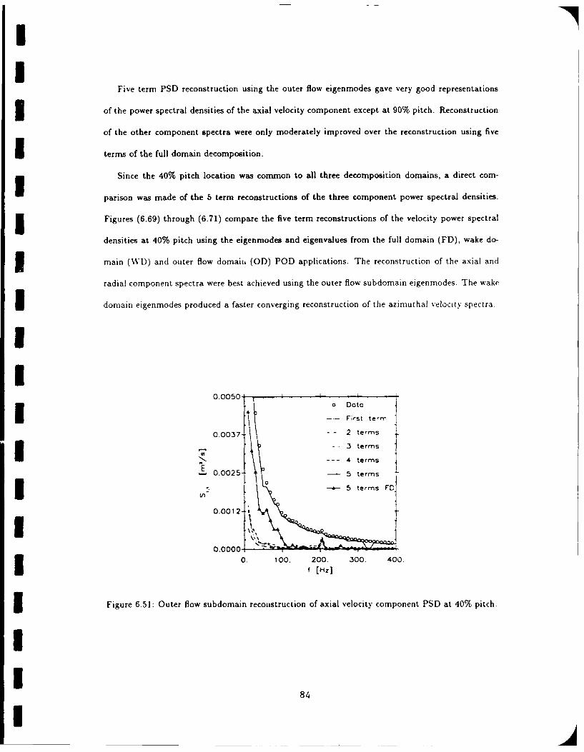
II

Five term PSD reconstruction using the outer flow eigenmodes gave very good representations

3 of the power spectral densities of the axial velocity component except at 90% pitch. Reconstruction

of the other component spectra were only moderately improved over the reconstruction using five

I terms of the full domain decomposition.

Since the 40% pitch location was common to all three decomposition domains, a direct com-

parison was made of the 5 term reconstructions of the three component power spectral densities.

3 Figures (6.69) through (6.71) compare the five term reconstructions of the velocity power spectral

densities at 40% pitch using the eigenmodes and eigenvalues from the full domain (FD), wake do-

3 main (WD) and outer flow domaiin (OD) POD applications. The reconstruction of the axial and

radial component spectra were best achieved using the outer flow subdomain eigenmodes. The wake

3 domain eigenmodes produced a faster converging reconstruction of the azimuthal velocity spectra.

II

0.0050-o DOtW

First term0.0037- -- 2 terms

I .... . ems

- 3 terms

- 0.0025 5 terms'0-- 5 terms FD

0.0000 0 . 10 0. 200. 300. 400

f IHz]

3 Figure 6.51: Outer flow subdomain reconstruction of axial velocity component PSD at 40% pitch.

II 84

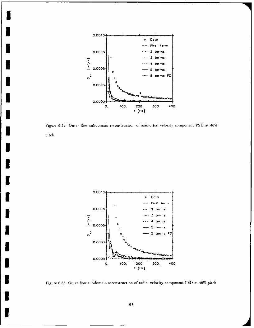
I

1 0.0010 0 Date0 Data

-- First term

0.0008 . 2 terms

S...3 terms9,

--- 4 terms

0.0005- - 5 terms0

- 5 terms FD

0.0003- 00o 00

00C-- O 000000O0000 oooooIooooooooooo

0 . 100. 200. 300. 400.If [Hz]

Figure 6.52: Outer flow subdomain reconstruction of azimuthal velocity component PSD at 40%

pitch.

III

0.0010-D t

0 Data-- First term

00.0008- -- 2 terms

.. 3 terms

--- 4 terms

0.0005 00 5 terms

on 00 5 terms FDo0

I 0.0003 00000I

0000 00000000000

0. 100. 200. 300. 400.

f [Hz]

I Figure 6.53: Outer flow subdomain reconstruction of radial velocity component PSD at 407 pitch.

885U

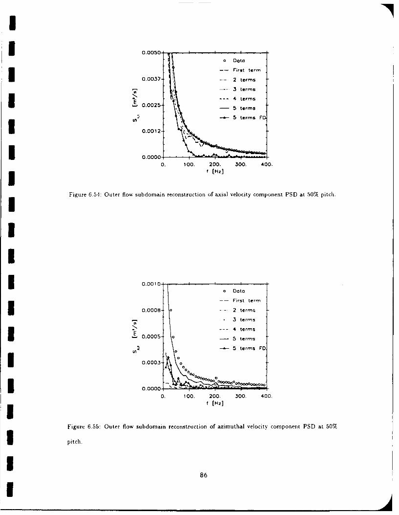
1 0.00500 Data

-- First term

0.0037-- - 2 terms

- 3 terms

* --- 4 terms

IE1 0.0000-

0. 100. 200. 300. 400.3 f [Hz]

Figure 6.54: Outer flow subdomain reconstruction of a-xial velocity component PSD at 50% pitch.

I 0.00 10-0 Dato

-- First termI 0.0008- 0 -- 2 terms- - 3 terms

-- 4 termsIE0.0005- 0 5 terms-- 5 terms FD

(A 00

0

0.0003

0.0000,

Figure 6.55: Outer flow subdomain reconstruction of azimuthal velocity component PSO at 50%

I pitch.

86

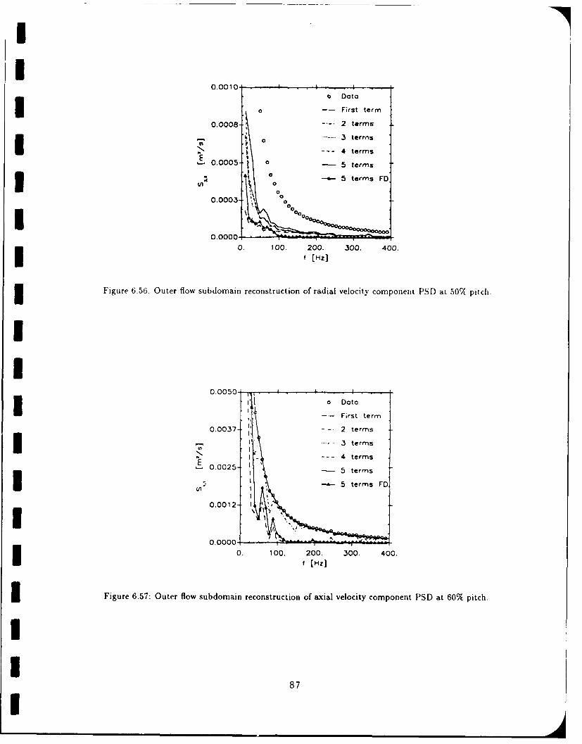
0.0010o DataU 0- First term

0.0008 - 2 terms-

2 terms- - - 4termsE 0.005' 0 -5 terms

- -.- 4 terms F0

0

0.0003 a~** (z

0. 10. 200. 300. 400.

Figure 6.56: Outer flow subdomain reconstruction of radial velocity component PSD at 50%, pitch.

0.0050o Data

-- First term

0.0037- - 2 terms

cn F -... 3terms

N. ----

4terms

0.0000

5 te m

0.010020030040

f[Hz]

Figure 6.57: Outer flow subdomain reconstruction of axial velocity component PSD at 60% pitch.

87

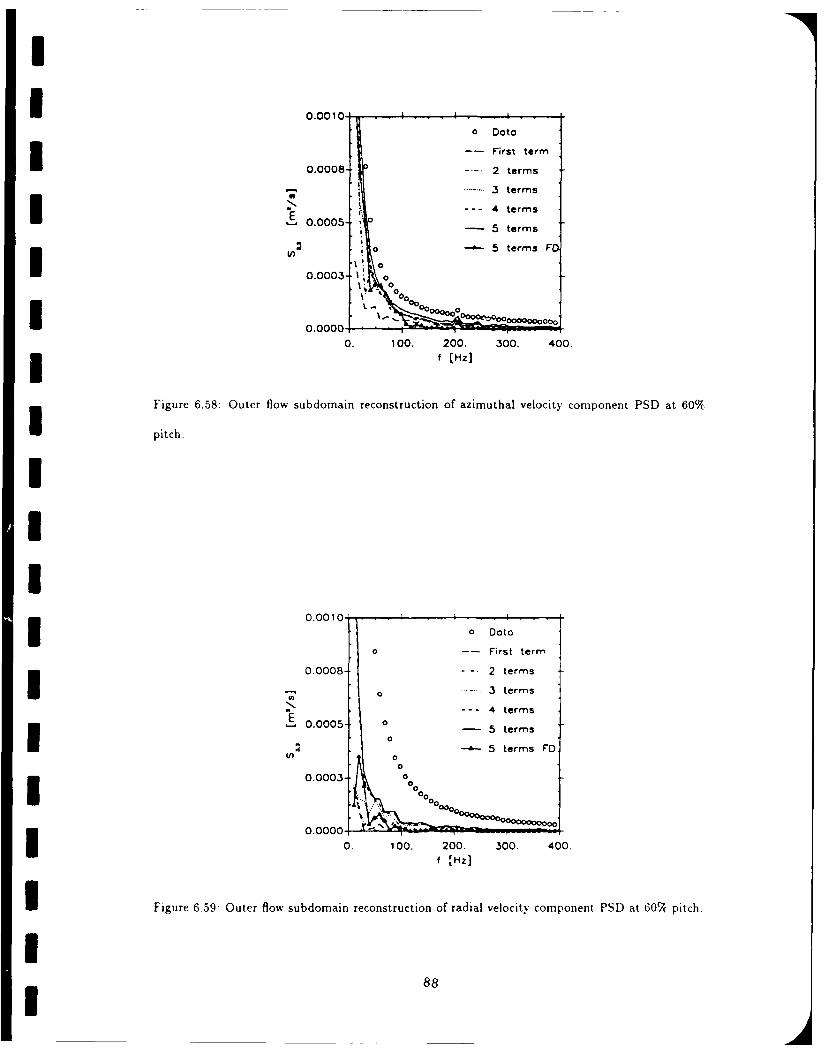
I

I 0.0010 , . 0 Dat .0 Data

-- First term

0.0008 . 2 terms

3 terms

0 0- - 4 terms*E 2 i0) 5 terms FD.

0.00031 00 -0

0 . 100. 200. 300. 400.f [Hz]

Figure 6.58: Outer flow subdomain reconstruction of azimuthal velocity component PSD at 60%

pitch.

I

0.00 10-

0 Data0 -- First term

0.0008 - - 2 terms

o -3 terms

4 terms

0.0005- 0 5 terms5 terms FD01 0

00.0003- 0

- 0O.000 100. 200. 300. 400.

[Hz

I Figure 6.59: Outer flow subdomain reconstruction of radial velocity component PSD at 60%, pitch.

8

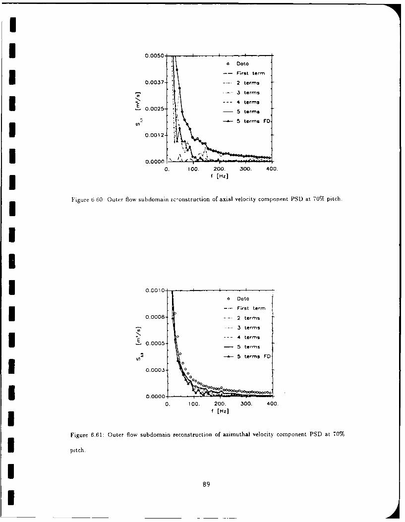
I ~ ~0.0050 I I

0 Data3-- First term0.0037-- 2 terms

3 terms4terms

E4I 0.0025- em

0. 100. 200. 300. 400.3 f [Hz]

Figure 6-60: Outer flow subdomain rc-onstruction of axial velocity component PSD at 707c pitch.

1 0.0010-o Dato

-- First term

0 4 terEsIs 0.00085. 2 terms

0t e 000.003 0em

0.0005- 50000m

-~ 000000 000..0I0.0000- 00. 0. 20 0. 403 f (Hz

Fiur 661 Ote lo sbdman eontrctonofazmthl elciy opoen PD t00I pitch

I089 .0U0000

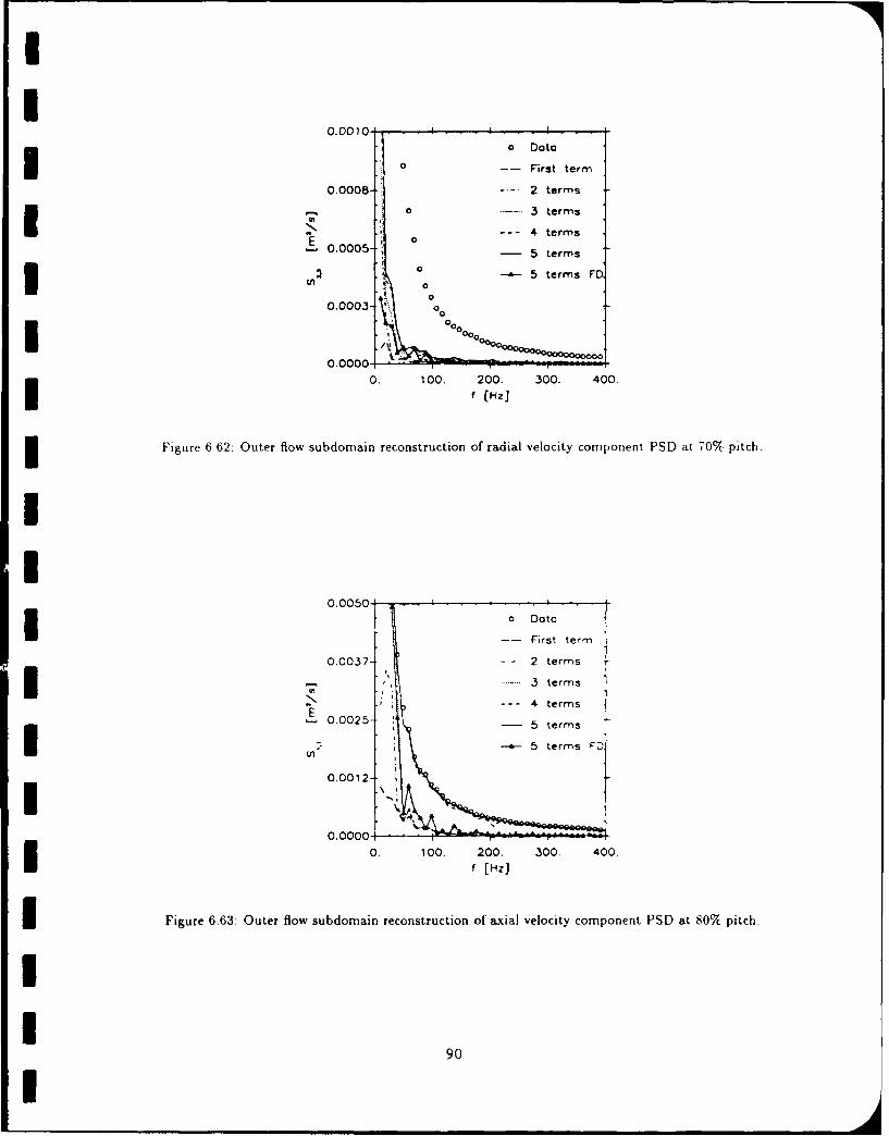
0 .0 0 1 0 -0 D t3 a - First term

0.0008-- 2 terms

0 3 terms

- - - -4 terms

0.0005-- 5 terms

0-'5 terms FOLA0

00

0

0 .0 0 . 1 0 0 . 2 0 0 . 3 0 0 . 4 0 0

Figure 6.62: Outer flow subdomain reconstruction of radial velocity component PSD at 70% pitch.

0.0050 oDato

-- First term

0.0037-- 2 terms

I"'3 terms'N.

-- - 4termsE 0 .0 0 2 5 -

e m

000 0. 100. 200. 300. 400.

IFigure 6.63: Outer flow subdomain reconstruction of axial velocity component PSD at 80% pitch.

90

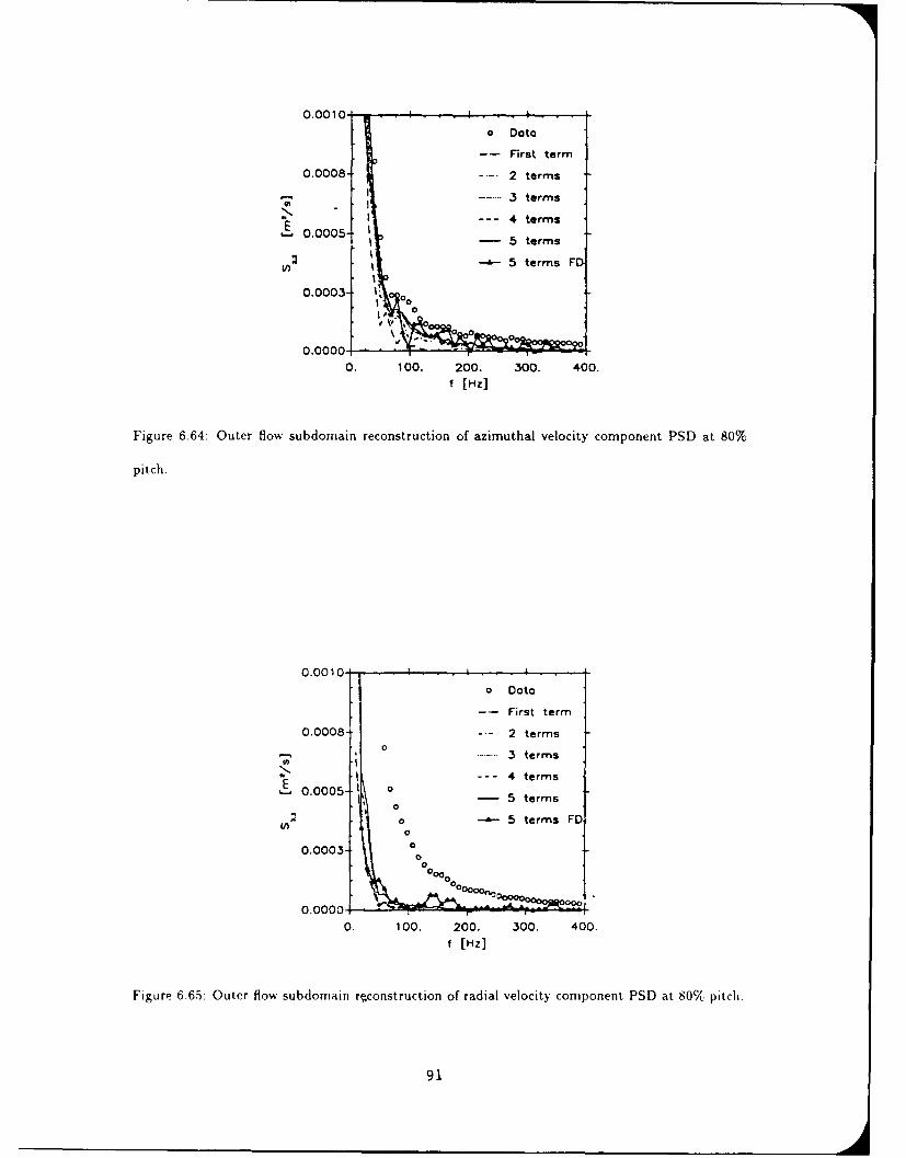
0.00 10- o Data

-- First term

0.0008-- 2 terms

3r terms

4 terms-5te

rms-- 5te rmsF

0.0005- 5 ter00

00

0.00000. 1 00. 20 30. 4.

0.00100 I

0.0008-- 2 terms

- *.*-0* 3 termsI 4 terms

E 0.0005- 0 -5 terms

11 0

w" 0 5 terms FD

0.0003- 0

0

0.0000- *'=M000

0. 100. 200. 300. 400.( Hz]

Figure 6.65: Outer flow subdomaiti reconstruction of radial velocity conmponent PSD at 807( pitch.

91

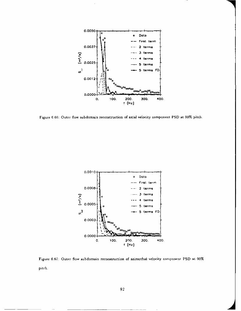
0.00500

o Data0

0 -- First term

0.0037-- 2 terms

- 3 terms

-- 4 termsE*0.0025-- 5 terms

0 -~5 terms FDWf

0.0012 00* 00

51 0000,000 I 0000

0000. 100. 200. 300. 400.f(HZ]

Figure 6.66: Outer flow subdomain reconstruction of axial velocity component PSD at 90% pitch.

0.0010-0 Data

-- First term

0.0008-- 2 terms

-3 terms

--- 4 termsE0.0005- 0 5 terms

1-'5-terms FD

0.0 0 3 0 0 ,0 0 0

0.000010. 100. 200. 300. 400.

f[Hz]

Figure 6.67: Outer flow subdomain reconstruction of azimuthal velocity component PSD at 90%X

pitch.

92

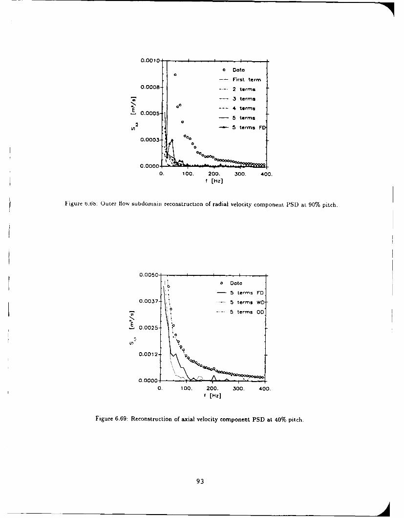
0.0010* 1o Data

0-- First term

0.0008- -- 2 terms

S...3 terms

000.0005

--- 4 terms

0005 terms

E--- 5 terms FD

0.0003- co0

0

o 00oo 0000

0.0000-'0. 100. 200. 300. 400.

f [Hz]

Figure b.66: Outer flow subdornain reconstruction of radial velocity component PSD at 90% pitch.

0,0050 _. I I I

0 Data

- 5 terms FD

0.0037- - 5 terms WD

- .. 5 terms O0

Ea 0.0025-

0.0012--

0. 100. 200. 300. 400.

f [Hz]

Figure 6.69: Reconstruction of axial velocity component PSD at 40% pitch.

93

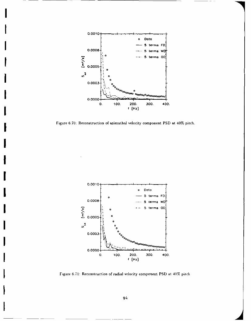
I

I 0.00 10 .- - -. .a Doto

I - 5 terms FD

0.0008 - 5 terms Wt"

.0 --. 5 terms 00m

E 0.0005-

0I 0.0003 ! 0

00

0.0000.

0 . 100. 200. 300. 400.i f [Hz]

Figure 6.70: Reconstruction of azimuthal velocity component PSD at 40% pitch.

0.0010 . I

o DOta

- 5 terms FD0.0008- • 5 terms WOI

.... 5 terms 00

,.0.0005-

LA 00.0003- 0

0 00000 0010.0000 ; -.- ... .. -

0. 100. 200. 300. 400.

f [Hz]

Figure 6.71: Reconstruction of radial velocity component PSD at 40% pitch

94

7 Conclusions and Recommendations

A more complete understanding of complex turbine flowfields is needed in order to improve on

the performance of mean-flow based turbine designs. To understand what is happening in the

turbine flowfield, it is essential to know how the turbulence is generated, how it propagates and

how it modifies the flow. While identifying turbulence contributions to signals, standard averaging

techniques (such as phase locked averaging) leave unanswered questions regarding the spatial and

temporal character of the turbulence itself. It was hypothesized at the beginning of this investigation

that there exist typical wake and passage flows which possess characteristics important to the rotor

dynamics. An investigation of the behavior and content of the hypothesized coherent structures

comprising the turbulence contribution to the turbine flowfield was therefore undertaken in this

study.

The proper orthogonal decomposition (POD), a technique proposed by Lumley (1967) for the

eduction of coherent structures, was selected for t',is study. The coherent structures are identified by

the POD as the set of orthonormal functions (modes) for which the mean square projection on the

flowfield is maximized. This method of structure identification was chosen because the dynamical

I evolution of the modes can be examined and calculated (v. George 1988 and r ft-rences therein).

The POD was applied to three component triple-wire probe spectral tensor n .asurements of a large-

scale annular stator model exit flowfield. This study represents the first application of the orthogonal

decomposition to directly measured three component data, and one of the first application to an

applied engineering flow.

The original research proposed to use cross-wire pro-s and measure the entire field in a plane at

the stator exit. However, since the radial flow component was not negligible or uniform, especially

in the wake region, it was decided to use trir!e-wire probes and directly measure all three velocity

components. This decision was not withr-t cost however, as long delays in the experimental program

were a consequence. As a result of these delays, together with the expiration of funding, the multi-

point triple-wire probe mea.s'jrements had to be limited to a midspan traverse of two probes across

95

one stator pitch at one axial location 10% axial chord downstream of the stator trailing edge

The POD was applied first to the entire set of 1089 cross-spectral estimates representing the

passage exit midspan. Reconstructions of the power spectral densities were examined to gauge

the merit of the POD modes to characterize the energy of the flowfield. Only a few POD modes

were required to represent a significant amount of the energy of the field (3 terms for over 50%

energy representation). Low frequency (below 200 Hz) spikes were found in the eigenmodes at

various frequencies aid were attributed to either inlet flow disturbances or meandering of coherent

structures generated by the blade row. Decomposition of other transverse measurement sets would

have assisted in identifying the origin of such spikes. Outside of the wake region, the modes typically

represent the energy at progressively higher frequencies and thus capture tile large scale structures

in the lowest modes. Within the wake however, the POD modes very effectively captured the high

frequency, high energy content. The eigenspectra for the full domain decomposition indicate that

the first four mode, essentially accomodated completely the high energy associated with the wake.

Moin and Moser (1989) and George and Glauser (1991) suggested applying the POD to subdo-

mains with inherently different flow regimes in order to increase the convergence rate of the energy

representation by the modes. This premise was based on Lumley's (1967) argument that the conver-

gence of the expansion in terms of energy is a function of the spatial extent divided by the integral

scale. In this study, outside of the hub and shroud boundary layers, the passage exit flow consists

primarily of two domains, the wake and the outer flow regions. Because of the large difference in

scales between these regions, the orthogonal decomposition was applied separately to the two do-

mains in order to see if better convergence of the expansion could be achieved. Convergence of the

POD was found to be affected by the flow regime contained in the domain. The eigenspectra and

eigenmodes of the subdomain which included the wake region had a similar character to those of the

full domain POD although their convergence was significantly better (2 terms for over 50% energy

representation). By applying the POD to a subdomain which excluded the wake, the convergence of

the subdomain energy representation was indicative of the expansion of a quasi-homogeneous field

(v. Chambers et al. 1988). The first mode represented only 17% of the domain energy and four

96

modes were required to provide over 50% energy reconstruction.

Since the POD eigenmodes have been shown to characterize a significant portion of the stator exit

flowfield energy (for the measurements of this study), it would be useful to determine the dynamics

of the structures which should relate to the downstream blade row dynamics. The dynamics of a

flowfield could be examined by reconstructing the instantaneous flowfield in terms of the POD modes

(Eq. (2.7)) and tracking the transfer of energy among the eigenmodes (v. George 1988 and George

and Glauser 1991). The data necessary for such a calculation using one dimensional flowfield cuts

would have to be taken with rakes of subminiature probes. An alternative approach would be the

application of the orthogonal decomposition to numerically simulated data.

The use of dynamical systems theory in conjunction with Galerkin projection of experimentally

determined modes on the Navier Stokes equations has been shown (v. Sirovich 1987, Aubrey et al.

1988 and Glauser et al. 1989) to be an effective means for investigating the dynamics of the flowfield

coherent structures. This method reduces the problem of finding the complex coefficients for the

velocity reconstruction (Eq. (2.7)) from a set of linear ordinary differential equations. To apply

this analysis, it is useful to apply the decomposition to the cross-spectral tensor defined in terms of

the cross-correlation tensor (mean in) as opposed to the covariance tensor (fluctuations only). In

this study the decomposition was applied only to the fluctuating field since solving the eigensystem

problem can easily be repeated with the entire flowfield at a later time.

To summarize, additional data is needed to ascertain the origin of coherent flowfield structures

in the stator exit flowfield and to determine their subsequent dynamics. With the increased compu-

tational capability, a combined experimental and computational effort is most likely to achieve the

desired objective of not only identifying proper orthogonal decomposition eigenfunctions but also

their dynamics and effects on downstream blade row dynamics.

97

II

-- 8 Publications

3 8.1 Directly Related to Work

George, W.K., P.D. Beuther and A. Shabbir (1989) "Polynomial Calibrations for Hot-Wires in

Thermally Varying Flows", J. of Exp. Thermal and Fluid Science 2:230-235.

3- George, W.K., H.J. Hussein and S.H. Woodward (1989)"An Evaluation of the Effect of a Fluctuating

Convection Velocity on the Validity of Taylor's Hypothesis", Australasian Fluid Mechanics Conf.

3U. of Melbourne, Australia, Dec. 11-15.

LeBoeuf, R.L. and \V.K. George (1990) "The Calibration and Use of Non- Orthogonal Cross-Wire3 Probes", ASME FED-Vol. 97. The Heuristics of Thermal Anemometry, Eds. D.E. Stock, S.A.

Sherif and A.J. Smits.

3LeBoeuf, R.L. and W.K. George (1990) "A New Approach to the Calibration of Non-Orthogonal

Triple-Wire Probes", Bulletin of the American Physical Society, V. 35, No. 10, 2274.

George, W.K. and M.N. Glauser (1991) "Multi-Point Measurements in Turbulence", to be published

in Proc. of 2nd World Congress on Heat Transfer, Fluid Mechanics and Thermodynamics, Elsevier.

N.Y.

8.2 Other Papers Published by Principals Bearing Some

Relation to Work

Rae, W.J., D.B. Taulbee, K.C. Civinskis and M.G. Dunn (1988) "Turbine Stage Heat Transfer: Coin-

parison of Short-Duration Measurements with State-of-the-Art Predictions", Journal of Propulsion

and Power. V.4, 541-548.

Taulbee, D.B. (1988) "Engineering Turbulence Models", Recent Advances in Turbulent Flows. eds.

W.K. George and R. Arndt, Hemisphere, pp. 75-125.

Taulbee, D.B. and L. Tran (1988) "Stagnation Streamline Turbulence", AIAA Journal, pp. 1011-

1013.

Taulbee, D.B., L. 'ran and M.G. Dunn (1988) "Stagnation Point and Surface Heat Transfer for

a Turbine Stage: Prediction and Comparison with Data", ASME International Gas Turbine and

Aeroengine Congress, Amsterdam, The Netherlands.

98

George, W.K. (1989) "A New Heat Transfer Law for Turbulent Natural Convection Between Heated1 Horizontal Surfaces of Large Extent", 26th ASME Nat. Heat Trans. Conf. and Exhib., Phil. Pa.

Aug. 6-9. (ASME 1989 HTD), 107, pp, 51-61.

IHussein, H. J. and W.K. George (1989) "Measurements of Small Scale Turbulence in an Axisym-

metric Jet Using Moving Hot Wires", Proc. of 7th Turbulent Shear Flow Conf., Stanford Univ.,3 Palo Alto, CA pp. 30.2.1 - 30.2.6.

George, W.K. and M.M. Gibson (1989) "Theory for Self-Preserving Homogeneous Turbulent Shear

Flow." Proc. of 7th Turbulent Shear Flow Conf., Stanford Univ. Palo Alto, CA pp. 27.1.1 - 27.1.6.

Han, Y. Oun and W.K. George (1989) "Turbulence Energy Budgets Through a Contraction", Proc.

u of Fluid Mech. Seminar, Korea-U.S. Progress, Taejon, Korea, Hemisphere. NY.

Lasher. W.C. and D.B. Taulbee (1989) "The Effect of the Near-Wall Treatment on the Behavior

of Reynolds Stress Turbulence Models for Reattaching Flows", 7th Symposium on Turbulent Shear

Flows, Stanford, CA.

Taulbee, D. B., L. Tran and M.G. Dunn (1989) "Stagnation Point and Surface Heat Transfer for a

Turbine Stage, Prediction and Comparison with Data", J. of Turbomachinery, V. 111, pp. 29-35.

Taulbee, D.B. and L. Tran (1989) "Prediction of Unsteady Rotor - Surface Heat Transfer from Wake

Passings", AISS 24th Thermophysics Conf., Buffalo, NY.

Tran L. and D.B. Taulbee (1989) "Prediction of Stagnation Point Heat Transfer with Free Stream

Turbulence", 1989 National Heat Transfer Conference, Phila. PA.

Glauser, M.N., X. Zheng and W.K. George (1990) "The Streamwise Evolution of Coherent Structures

in the Axisymmetric Jet Mixing Layer", The Lumley Symposium, Newport News, VA. Nov. 11-13,

Ed. Springer-Verlag.

George, W.K. and D.B. Taulbee (1990) "Designing Experiments to Test Closure Hypotheses," Pro-

ceedings of the International Symposium on Engineering Turbulence Modelling and Measurements,

Dubrovnik, Yugoslavia, Sept. 24-28, ed. W. Rodi and E.N. Ganic, Elsevier Publishing Co., New

York, pp. 383-397.

George, W.K. (1990) "Graduate Education in Turbulence: An Opinion" , AFOSR Symposium on

Turbulence in the 90's. Princeton University, Sept. 1990.

99

II

Appendix A

U POD Formulation

The extremization of A in Eq. (2.3) can be found by considering a function in the neighborhood of

3 the maximizing function 0,(.)

)= ',() + f(-) (A.1)

I where ( is an infinitesimal parameter and q?(.) is well behaved with appropriate boundary conditions.

3 With substitution of Eq. (A.1) with the appropriate conjugation and independent variable into

Eq. (2.3), the extremum can be found using the usual method of differential calculus, ie. by setting

I k dE(_d =0. (A.2)

I Evaluation of Eq. (A.2) for A given by Eq. (2.3) yields

J [+()+(.') +0,.')?7(.))d.- .')=(.)d(.') -0A-f,( .) +,. ) =o. (A.3)

Substitution of (7) = (.) and (:') = (.1) followed by the substitutions '-) = (.) and (-') = ()

3effectively switches the independent variable in an expression. Applying these substitutions and

using the identity

R j7(", -) = n ,.j(., . (A.4)

for the first term only in Eq. (A.3) yields

J {[k(.')ri(.)R .(..') + 6i()O'(.Rij(., ')]d(.')-A[fr(.)"(.) + ((.)]}d(.)=O. (A.5)

Since the integral over (.) is for arbitrary bounds, the integrand is itself zero. Factoring rt(.) and

5 r17(.) out of the resulting equation yields

n( )I 0 (.')R ij(., .')d(.') - AO;(.)] + A' . ¢ ( ) A ,.) (-' .A)] = 0 (A .6)

3 which is the sum of complex conjugates. Since the auxiliary function 17(.) is well behaved and non-

zero, the bracketed terms must themselves be identically zero. Further manipulation of either term

i100

I

II

yields the integral equation

I f R~(., .')4 3(.')d(.') = A~,(.) (Al)

which can be solved for the deterministic, but randomly distributed candidate functions ~i.

UUIIIIIIIIIIII 101

I

Bibliography

Adrian, R.J., 1979, "Conditional Eddies in Isotropic Turbulence," Physics of Fluids, Vol. 22, pp.

2065-2070.

3 Andreopoulos, ., 1983, "Improvements of the Performance of Triple Hot Wire Probes," Rev. Sci.

Instrum., Vol. 54(6), pp. 733-740.

3 Andreopoulos, J., 1983, "Statistical Errors Associated with Probe Geometry and Turbulence Inten-

sity in Triple Hot-Wire Anemometry," J. Phys. E: Sci. Instrum., Vol. 16, pp. 1264-1271.

i Antonia, R.A., 1981, "Conditional Sampling in Turbulence Measurement," Ann. Rev. Fluid Niech.,

Vol. 13, pp. 131-156.

U Aubry, N., Holmes, P., Lumley, J.L. and Stone, E., 1988, "The Dynamics of Coherent Structures in

the Wall Region of a Turbulent Boundary Layer," J. Fluid Mechanics, Vol. 192, pp. 115-173.

Bailey, D.A., 1979, "Study of Mean- and Turbulent- Velocity Fields in a Large-Scale Turbine-Vane

3 Passage," NASA Contractor Report 3076.

Baker, C.T.H., 1977, The Numerical Treatment of Integral Equations, Clarendon Press, Oxford.

I Bakewell. H.P., and Lumley. J.L.. 1967, "Viscous Sublayer and Adjacent Wall Region in Turbulent

Pipe Flow," The Physics of Fluids, Vol. 10, No. 9, pp. 1880-1889.

I Beuther, P.D., 1980, Experimental Invesligation of the Axzisymmetric Turbulent Buoyant Plume,

Ph.D. Dissertation, SUNY at Buffalo.

Beuther, P.D., Shabbir, A. and George, W.K., 1987, "X-Wire Response in Turbulent Flows of High-3Intensity Turbulence and Low Mean Velocities," ASME Symposium on Thermal Anemometry - FED

- Vol. 53, Ed. D.E. Stock.

Blair, M.F., Dring, R.P. and Joslyn, H.D., 1989a, "The Effects of Turbulence a:,d Stator/Rotor Inter-

actions on Turbine Heat Transfer: Part -Design Operating Conditions," ASME J. Turbomachinery,

Vol. 111, pp. 87-96.

Blair, M.F., Dring, R.P. and Joslyn, H.D., 1989b, "The Effects of Turbulence and Stator/Rotor

Interactions on Turbine Heat Transfer: Part II-Effects of Reynolds Number and Incidence," ASME

J. Turbomachinery, Vol. 111, pp. 97-103.

102

Bruun, H.H., 1979, "Interpretation of Hot-Wire Probe Signals in Subsonic Airflows," J. Phys. E:

Sci. Instrum., Vol. 12, pp. 1116-1128.

Butler,T.L. and Wagner, JW., 1983, "Application of a Three-Sensor Hot-Wire Probe for Incom-

pressible Flow," AIAA Journal, Vol. 21, No. 5, pp. 726-732.

Chambers, D.H., Adrian, R.J., Moin, P., Stewart, D.S. and Sung, H.J., 1988, "Karhunen-Lo6ve

Expansion of Burgers' Model of Turbulence," Phys. Fluids, Vol. 31 (9), pp. 2573-2582.

Champagne, F.H., Sleicher, C.A. and Wehrmann, O.H., 1967, "Turbulence Measurements with

Inclined Hot-Wire, Part 1. Heat Transfer Experiments with Inclined Hot-Wire," J. Fluid Mech. 28

Part 1, pp. 153-175.

Dring. R.P., Joslyn, H.D. and Blair, M.F., 1987, "The Effects of Inlet Turbulence and Rotor/Stator

Interactions on the Aerodynamics and Heat Transfer of a Large-Scale Rotating Turbine Model;

IV-Aerodynamic Data Tabulation," NASA Contractors Report 179469.

Dring, R.P., Joslyn, H.D., Hardin, L.W. and Wagner, J.H., 1982, "Turbine Rotor-Stator Interaction,"

ASME J. Engineering for Power, Vol. 107, pp. 729-742.

Dring, R.P., Blair, M., Joslyn, H.D., Power, G.D. and Verdon, J.M., 1986, "The Effects of Inlet

Turbulence and Rotor/Stator Interactions on the Aerodynamics and Heat Transfer of a Large-Scale

Rotating Turbine Model; I-Final Report," NASA Contractor Report 4079.

Dunn, M.G., 1986, "Heat-Flux Measurements for the Rotor of a Full-Stage Turbine: Part I-Time-

Averaged Results," ASME Paper No. 86-GT-77.

Dunn, M.G., George, W.K., Rae, W.J., Woodward, S.H., Moller, J.C. and Seymour, P.J., 1986,

"Heat Flux Measurements for the Rotor of a Full-Stage Turbine: Part ll-Description of Analysis

Technique and Tynical Time-Resolved Measurements," ASME Paper No. 86-GT-78.

Dunn, M.G., Bennett, W., DeLaney, R. and Rao, 1990, "Investigation of Unsteady Flow Through

a Transonic Turbine Stage, Parts II and III: Comparison of Time-Averaged and Phase Resolved

Heat-Flux Data on Blade and Vane with Predictions," AIAA Paper No. 90-2409 and 90-2410.

Evans, R.L., 1975, "Turbulence and Unsteadiness Measurements Downstream of a Moving Blade

Row," ASME J. Engineering for Power, pp. 131-139.

Fabris, G., 1978, "Probe and Method for Simultaneous Measurement of "True" Instantaneous Tem-

perature and Three Velocity Components in Turbulent Flow," Rev. Sci. Instrum., Vol. 49, No. 5.

103

George, W.K., 1988, "Insight into the Dynamics of Coherent Structures from a Proper Orthogonal

Decomposition," Proceedings Symposium on Near Wall Turbulence, Dubrovnic, Yugoslavia, May

16-20.

George, W.K., Beuther, P.D. and Lumley, J.L., 1978, "Processing of Random Signals," Proceedings

of the Dynamic Flow Conference.

George, W.K., Beuther, P.D. and Shabbir, A., 1987, "Polynomial Calibrations for Hot Wires in

Thermally-Varying Flows," ASME Symposium on Thermal Anemometry - FED - Vol. 53, pp. 1-6.

George, W.K. and Glauser, M.N., 1991, "Flow Structure Identification From Multi-Point Measure-

ments," 2nd World Conference on Heat Transfer, Fluid Mechanics and Thermodynamics, Dubrovnic,

Yugoslavia, June.

Glauser, M.N., 1987, Coherent Structures in the Aznsymmetric Turbulent Jet Mixing Layer, Ph.D.

Dissertation, SUNY at Buffalo

Glauser, NI., Zheng, X. and Doering, C.R., 1989, Turbulence and Coherent Structures, Kluwer

Academic Publishers.

Gorton, C.A. and Lakshminarayana, B., 1976, "A Method of Measuring the Three-Dimensional

Mean Flow and Turbulence Quantities Inside a Rotating Turbo-Machinery Passage." ASME J.

Engineering for Power, pp. 137-146.

Graham, R.W., 1980, "Fundamental Mechanisms That Influence the Estimate of Heat Transfer to

Gas Turbine Blades," Heat Transfer Engineering, Vol. 2, No. 1, pp. 39-47.

Graziani, R.A., Blair, M.F., Taylor, J.R. and Mayle, R.E., 1980, "An Experimental Study of Endwall

and Airfoil Surface Heat Transfer in a Large Scale Turbine Blade Cascade," ASME J. Engineering

for Power, Vol. 102, pp. 257-267.

Gregory-Smith, D.G. and Graves, C.P., 1983, "Secondary Flows and Losses in a Turbine Cascade,"

Viscous Effects in Turbomachines, AGARD CP 351.

Guenette, G.R., Epstein, A.H., Giles, M.B., Haimes, R. and Norton, R.J.G., 1989, "Fully Scaled

Transonic Turbine Rotor Heat Transfer Measurements," ASME J. Turbomachinery, Vol. 111, pp. 1-

7.

Herzog, S., 1986, The Large Scale Structure in the Near- Wall Region of Turbulent Pipe Flow, Ph.D.

Dissertation, Cornell University.

Hinze, J.O., 1959, Turbulence, McGraw-Hill, New York.

104

Hodson, H.P., 1985, "Measurements of Wake Generated Unsteadiness in the Rotor Passages of Axial

Flow Turbines," ASME J. Engineering for Gas Turbines and Power, Vol. 107, pp. 467-476.

Jorgenson, F.E., 1971, "Directional Sensitivity of Wire and Fiber-film Probes," DISA Information,

No. 11, pp. 31-37.

Junkins, J.L., 1978, An Introduction to Optimal Estimation of Dynamical Systems, Sijthoff and

Noordhoff, Alphen aan den Rijn, The Netherlands.

Ketter, R.L. and Prawel, S.P., 1969, Modern Methods of Engineering Computation, McGraw-Hill

Book Co., New York.

King, L.V., 1914, "On the Convection of Heat From Small Cylinders in a Stream of Fluid: De-

termination of the Convection Constants of Small Platinum Wires with Applications to Hot-Wire

Anemometry," Phil. Soc. A., 214, pp. 373-432.

LeBoeuf, R.L., 1990, "A New Approach to the Calibration of Non-Orthogonal Triple-Wire Probes,"

Presented at American Physical Society, Forty-Third Annual Meeting of the Division of Fluid Dy-

namics, Cornell University.

LeBoeuf, R.L. and George, W.K., 1990, "The Calibration and Use of Non-Orthogonal Cross-Wire

Probes," ASME FED-Vol. 97, The Heuristics of Thermal Anemometry. Eds. D.E. Stock, S.A. Sherif

and A.J. Smits, pp. 59-63.

Lekakis, I.C., Adrian, R.J. and Jones, B.G., 1989, "Measurement of Velocity Vectors With Orthog-

onal and Non-Orthogonal Triple-Sensor Probes," Experiments in Fluids, Vol. 7, pp. 228-240.

Lo6ve, M., 1955, Probability Theory, Van Nostrand, New York.

Lovitt, W.V., 1950, Linear Integral Equations, Dover Publications Inc., New York.

Lumley, J.L., 1967, "The Structure of Inhomogeneous Turbulent Flows," Atmospheric Turbulence

and Radio Wave Propagation, Nauka, Moscow.

Lumley, J.L., 1970, Stochastic Tools in Turbulence, Academic Press Inc., New York.

Mayle, R.E., 1991, "The Role of Laminar-Turbulent Transition in Gas Turbine Engines," ASME

Paper No. 91-GT-261, Presented at the International Gas Turbine and Aeroengine Congress and

Exposition, Orlando, Florida, June 3-6.

Moin, P. and Moser, R.D., 1989, "Characteristic-Eddy Decomposition of Turbulence in a Channel,"

J. Fluid Mech., Vol. 200, pp. 471-509.

105I

Moore, J. and Adhye, R.Y., 1985, "Secondary Flows and Losses Downstream of a Turbine Cascade,"

ASME J. Engineering for Gas Turbines and Power, Vol. 107, pp. 961-968.

Moustapha, S.H., Paron, G.J. and Wade, J.H.T., 1985, "Secondary Flows in Cascades of Highly

Loaded Turbine Blades," ASME J. Engineering for Gas Turbines and Power, Vol. 107, pp. 1031-

1038.

Oppenheim, A.V. and Willsky, A.S., 1983, Signals and Systems, Prentice-Hall, Englewood Cliffs,

New Jersey.

Raj, R. and Lakshminarayana, B., 1973, "Characteristics of the Wake Behind a Cascade of Airfoils,"

J. Fluid Mechanics, Vol. 61, Part 4, pp. 707-730.

Sharma, O.P., Butler, T.L., Joslyn, H.D. and Dring, R.P., 1985, "Three-Dimensional Unsteady Flow

in an Axial Flow Turbine," AIAA 3. Propulsion and Power, Vol. 1, No. 1, pp. 29-38.

Sidall, R.G. and Davies, T.W., 1972, "An Improved Response Equation for Hot-Wire Anemometry,"

Int. J. Heat Mass Trans., 15, pp. 367-368.

Sieverding, C.H., 1985, "Recent Progress in the Understanding of Basic Aspects of Secondary Flows

in Turbine Blade Passages," ASME J. Engineering for Gas Turbines and Power, Vol. 107, pp.

248-257.

Sieverding, C.H., Van Hove, W. and Boletis, E., 1984, "Experimental Study of the Three-Dimensional

Flow Field in an Annular Turbine Nozzle Guidevane," ASME J. Engineering for Gas Turbines and

Power, Vol. 106, pp. 437-444.

Sirovich, L., Maxey, M and Tarman, H., 1987, "Analysis of Turbulent Thermal Convection," 6th

Symposium on Turbulent Shear Flows.

Smith, B.T., Boyle, 3.M., Dongarra, J.J., Garbow, B.S., Klema, V.C. and Moler, C.B., 1976, Afaruz

Eigensystem Routines - EISPACK Guide, Springer-Verlag, New York.

Swaminathan, M.K., Rankin, G.W. and Sridhar, K., 1984, "Some Studies on Hot-Wire Calibration

Using Monte Carlo Technique," J. Phys. E: Sci. Instrum., 17, pp. 1148-1151.

Tan-atichat, J. and George, W.K., 1985, "Use of Computer for Data Aquisition and Processing,"

Handbook of Fluids and Fluid Machinery, John Wiley & Sons, Inc., Allen E. Fuhs, ed.

Tennekes, H. and Lumley, J.L., 1972, A First Course in Turbulence, The MIT Press, Cambridge,

Massachussettes.

Touloukian, Y.S., Saxena, S.C. and Hestermans, P., 1975, Viscosity, IFI/Plenum, New York.

106

I!

ITouloukian, Y.S., Liley, P.E. and Saxena, S.C., 1970, Thermal Conductivity: Nonmetallic Liquids

and Gases, IFI/Plenum, New York.

Treaster, A.L. and Houtz., H.E., 1986, "Fabricating and Calibrating Five-Hole Probes," presented at

the AIAA/ASME 4th Fluid Mechanics, Plasma Dynamics, and Lasers Conference, Atlanta, Georgia,

May 11-14.

I Treaster, A.L. and Yocum, A.M., 1979, "The Calibration and Application of Five-Hole Probes," ISA

Transactions, Vol. 18, No. 3.

I Ukeiley, L., Varghese, M., Glauser, M. and Valentine, D., 1991, "An Examination of Coherent

Structures in a Lobed Mixer Using Multifractal Measures in Conjunction with the Orthogonal De-

composition," AIAA Paper 91-0521.

Ukeiley, L., Wick, D. and Glauser, M., 1990, "A Novel Hot-Wire Rake Design," ASME FED-Vol.

97, The Heuristics of Thermal Anemometry, Eds. D.E. Stock, S.A. Sherif and A.J. Smits, pp. 87-92.

Webster, C.A.G., 1962, "A Note on the Sensitivity to Yaw of a Hot-Wire Anemometer," J. Fluid

Mech., 13, pp. 307-312.

Welz, J.P., 1986, "An Algorithm for Using the Five-Hole Probe in the Nonnulled Mode," presented at

the AIAA/ASME 4th Fluid Mechanics, Plasma Dynamics, and Lasers Conference, Atlanta, Georgia,

May 11-14.

107

I!