Advanced Modeling 2

Katja Buhler, Andrej Varchola, Eduard Groller

March 24, 2014

1 Parametric Representations

A parametric curve in E3 is given by

c : c(t) =

x(t)y(t)z(t)

; t ∈ I = [a, b] ⊂ R

where x(t), y(t) and z(t) are differentiable functions in t. The vector c iscalled tangent vector. A curve point c(t0), t0 ∈ I is called regular if c(t0) 6= o.

A parametrization is called regular, if c(t) 6= o for all t ∈ I. Any dif-ferentable change of the parameter τ = τ(t) does not change the curve.Moreover, if τ 6= 0 in I then d(t) = c(τ(t)) is also a regular parametrization.A curve which admits a regular parametrization is called regular.

A parametric surface is given by

s : s(u, v) =

x(u, v)y(u, v)z(u, v)

, (u, v) ∈ [a, b]× [c, d] = I × J ⊂ R2

where x(u, v), y(u, v) and z(u, v) are differentiable functions of the parame-ters u and v.

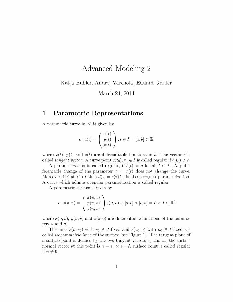
The lines s(u, v0) with v0 ∈ J fixed and s(u0, v) with u0 ∈ I fixed arecalled isoparametric lines of the surface (see Figure 1). The tangent plane ofa surface point is defined by the two tangent vectors su and sv, the surfacenormal vector at this point is n = su × sv. A surface point is called regularif n 6= 0.

1

For a good introduction to differential geometry see e.g. the book byAumann and Spitzmueller [1]. A detailed discussion of the following topicscan be found in the literature listed at the end of this summary. Almost allpictures are generated with the help of a collection of CAGD-Java appletswritten by the Geometric Design Group at the University of Karlsruhe:

http ://i33www.ira.uka.de/applets/mocca/html/noplugin/inhalt.html

Figure 1: Surface with Isolines

2 Bezier Curves

2.1 The Constructive Approach: The de Casteljau Al-gorithm

First described by de Casteljau it is probably the most fundamental algorithmin the field of curve and surface design, not least because it is so easy tounderstand. ”Its main attraction is the beautiful interplay between geometryand algebra: a very intuitive geometric construction leads to a powerfultheory”[2].

The AlgorithmGiven n+ 1 points b0, ..., bn ∈ E3 and an arbitrary t ∈ R. Then

bri = (1− t)br−1i + tbr−1

i+1 , r = 1, ..., n; i = 0, ..., n− r (1)

2

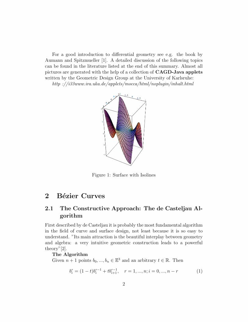
and b0i = bi, defines the point bn0 with parameter value t on the so calledBezier curve b(t). The points bi are called Bezier points.

Equation 1 describes a repeated linear interpolation whose intermediatecoefficients can be written into the triangular de Casteljau scheme (see Figure2):

b00b10

b01 b20b11 b30

b02 b21b12

b03

Figure 2: De Casteljau scheme

2.2 The Analytical Approach: Bezier Curves and Bern-stein Polynomials

The de Casteljau algorithm gives a recursive definition of Bezier curves interms of an algorithm. For further theoretical development it is also necessaryto have an explicit parametric representation for them. Based on the de

3

Casteljau recursion it can be shown by mathematical induction, that a Beziercurve b(t) with respect to the Bezier points bi, i = 0, ..., n is given by

b(t) =n∑

i=1

biBni (t)

where Bni (t) =

(ni

)(1 − t)n−iti are the Bernstein Polynomials of n-th degree

with the following important properties

� partition of unity:∑n

i=0Bni (t) ≡ 1

� positivity: Bni (t) > 0

� recursion: Bni (t) = (1− t)Bn−1

i (t) + tBn−1i+1 (t)

2.3 Some Properties of Bezier Curves

� Affine invariance: An affine transformation of the Bezier points is equiv-alent to an affine transformation of the whole curve.

� Convex hull property: A Bezier curve lies inside the convex hull of itsBezier points.

� Endpoint interpolation: The first and last Bezier points lie on the curve.

� Linear precision: If all Bezier points lie on a straight line, the corre-sponding Bezier curve is identical to this line.

� Variation diminishing property: A Bezier curve has no more intersec-tions with a plane than its Bezier polygon.

Disadvantage of Bezier curves:

� Pseudo local control: changing one of the control points changes theshape of the whole curve, although, if for instance bi is changed, it ismostly affected around the point corresponding to the parameter valuei/n, if n denotes the algebraic degree of the parametrization.

� The degree of a Bezier curve depends directly on the number of controlpoints. Thus, higher flexibility through more control points is equiva-lent to a higher degree of the curve, which means higher computationalcost and less control on the behavior of the curve.

4

2.4 Derivatives

It can be easily shown, that

� the lines b0b1 and bn−1bn are the tangent lines at the curve points b0and bn

� the intermediate points bn−10 and bn−1

1 of the de Casteljau algorithmdetermine the tangent line at the position bn0 (t).

2.5 Important Algorithms

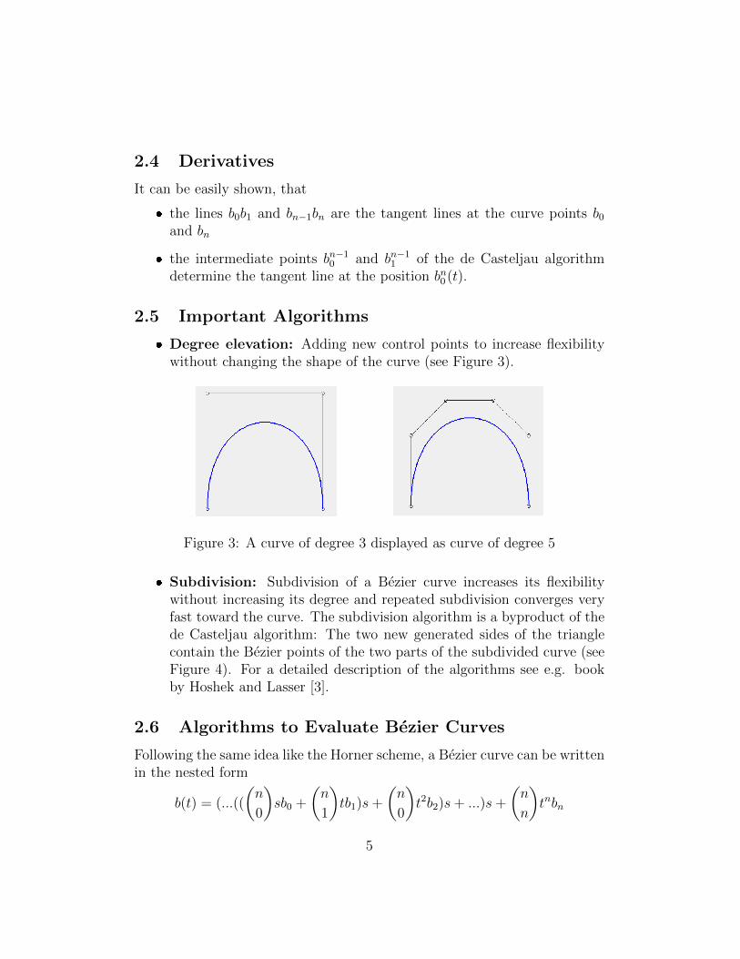
� Degree elevation: Adding new control points to increase flexibilitywithout changing the shape of the curve (see Figure 3).

Figure 3: A curve of degree 3 displayed as curve of degree 5

� Subdivision: Subdivision of a Bezier curve increases its flexibilitywithout increasing its degree and repeated subdivision converges veryfast toward the curve. The subdivision algorithm is a byproduct of thede Casteljau algorithm: The two new generated sides of the trianglecontain the Bezier points of the two parts of the subdivided curve (seeFigure 4). For a detailed description of the algorithms see e.g. bookby Hoshek and Lasser [3].

2.6 Algorithms to Evaluate Bezier Curves

Following the same idea like the Horner scheme, a Bezier curve can be writtenin the nested form

b(t) = (...((

(n

0

)sb0 +

(n

1

)tb1)s+

(n

0

)t2b2)s+ ...)s+

(n

n

)tnbn

5

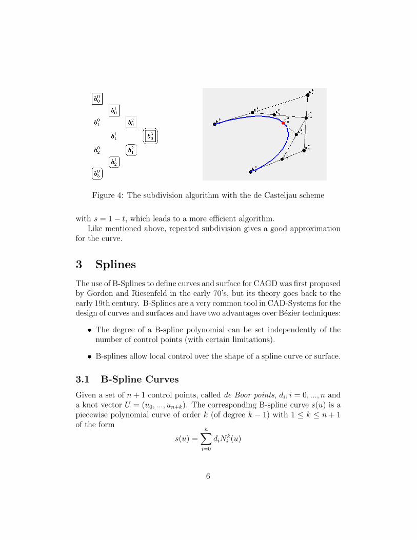
Figure 4: The subdivision algorithm with the de Casteljau scheme

with s = 1− t, which leads to a more efficient algorithm.Like mentioned above, repeated subdivision gives a good approximation

for the curve.

3 Splines

The use of B-Splines to define curves and surface for CAGD was first proposedby Gordon and Riesenfeld in the early 70’s, but its theory goes back to theearly 19th century. B-Splines are a very common tool in CAD-Systems for thedesign of curves and surfaces and have two advantages over Bezier techniques:

� The degree of a B-spline polynomial can be set independently of thenumber of control points (with certain limitations).

� B-splines allow local control over the shape of a spline curve or surface.

3.1 B-Spline Curves

Given a set of n+ 1 control points, called de Boor points, di, i = 0, ..., n anda knot vector U = (u0, ..., un+k). The corresponding B-spline curve s(u) is apiecewise polynomial curve of order k (of degree k − 1) with 1 ≤ k ≤ n+ 1of the form

s(u) =n∑

i=0

diNki (u)

6

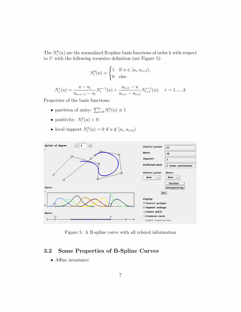
The Nki (u) are the normalized B-spline basis functions of order k with respect

to U with the following recursive definition (see Figure 5):

N0i (u) =

{1 if u ∈ [ui, ui+1),

0 else.

N ri (u) =

u− uiui+r−1 − ui

N r−1i (u) +

ui+r − uui+r − ui+1

N r−1i+1 (u); r = 1, ..., k

Properties of the basis functions:

� partition of unity:∑n

i=0Nki (u) ≡ 1

� positivity: Nki (u) > 0

� local support Nki (u) = 0 if u /∈ [ui, ui+k)

Figure 5: A B-spline curve with all related information

3.2 Some Properties of B-Spline Curves

� Affine invariance

7

� Strong convex hull property: The curve segment corresponding to theparameter values [ui;ui+1) lies inside the convex hull of the controlpoints di−k, ..., di.

� Variation diminishing property.

� Local support: Moving di changes s(u) only in the parameter interval[ui;ui+1).

� Multiple knot points ui = ... = ui+s are possible. If s ≥ k the curvegoes through the control point di. Furthermore if n = k − 1 andU = (u0, ..., u0, u1, ..., u1) then s(u) is a Bezier curve.

� Differentiability: s(u) is k− l− 1 times differentiable at a knot ui, if uiis of multiplicity l ≥ 1.

3.3 Some Special Types of B-Spline Curves

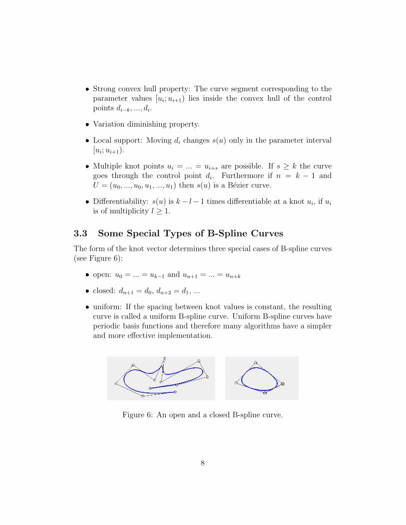
The form of the knot vector determines three special cases of B-spline curves(see Figure 6):

� open: u0 = ... = uk−1 and un+1 = ... = un+k

� closed: dn+1 = d0, dn+2 = d1, ...

� uniform: If the spacing between knot values is constant, the resultingcurve is called a uniform B-spline curve. Uniform B-spline curves haveperiodic basis functions and therefore many algorithms have a simplerand more effective implementation.

Figure 6: An open and a closed B-spline curve.

8

3.4 Evaluating B-Spline Curves

3.4.1 The de Boor algorithm

The de Boor algorithm is a generalized de Casteljau algorithm and worksfollowing the same principles as linear interpolation. To evaluate s(u) atu = u, u ∈ [ul;ul+1) the following recursion has to be done:

dri = (1− αri )d

r−1i−1 + αr

idr−1i , i = l − k + 1, ..., l; r = 0, ..., k − 1

with

αri =

u− uiui+k−r − ui

where d0i = di and s(u) = dk−1l . The de Boor scheme has the same form

like the de Casteljau scheme. The de Boor algorithm allows the evaluationof the curve, without any knowledge of the basis functions and proposes aneffective method.

3.4.2 The direct evaluation

A second possibility to evaluate a B-Spline function for a parameter value uis given by the following algorithm.

1. Find the knot span [ui, ui+1) in which u lies.

2. Compute the non zero basis functions.

3. Multiply the values of the nonzero basis functions with the correspond-ing control points.

3.5 Algorithms

Knot insertion and knot refinementThe knot insertion algorithm inserts a knot one or multiple times into the

knot vector (see Figure 7). Knot insertion does not change the shape of thecurve, but refines its segmentation. This algorithm is used to increase theflexibility of a curve, to compute derivatives, to split curves and to evaluatea curve for a certain parameter value: The de Boor algorithm is a repeatedknot insertion algorithm that inserts this parameter value k + 1 times intothe knot vector. There exist special algorithms that insert several differentknots simultaneously (knot refinement).

9

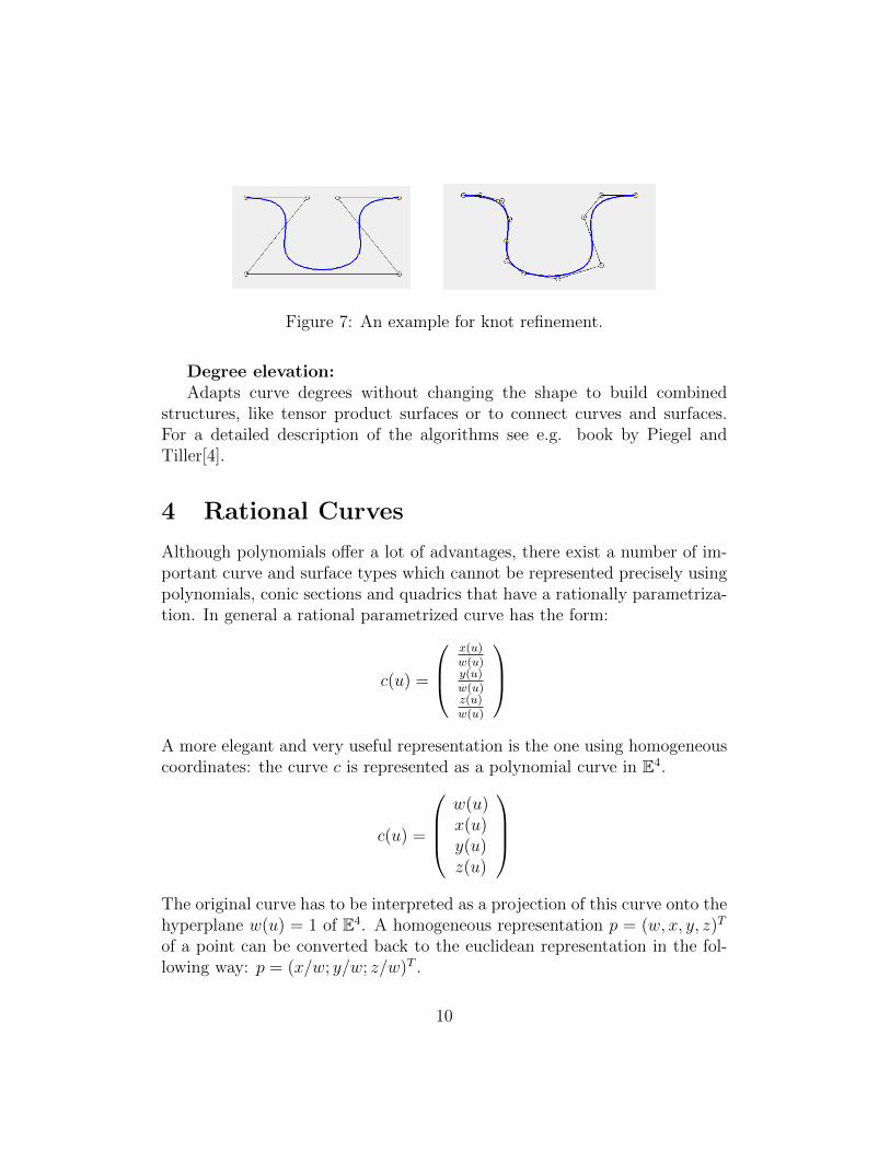
Figure 7: An example for knot refinement.

Degree elevation:Adapts curve degrees without changing the shape to build combined

structures, like tensor product surfaces or to connect curves and surfaces.For a detailed description of the algorithms see e.g. book by Piegel andTiller[4].

4 Rational Curves

Although polynomials offer a lot of advantages, there exist a number of im-portant curve and surface types which cannot be represented precisely usingpolynomials, conic sections and quadrics that have a rationally parametriza-tion. In general a rational parametrized curve has the form:

c(u) =

x(u)w(u)y(u)w(u)z(u)w(u)

A more elegant and very useful representation is the one using homogeneouscoordinates: the curve c is represented as a polynomial curve in E4.

c(u) =

w(u)x(u)y(u)z(u)

The original curve has to be interpreted as a projection of this curve onto thehyperplane w(u) = 1 of E4. A homogeneous representation p = (w, x, y, z)T

of a point can be converted back to the euclidean representation in the fol-lowing way: p = (x/w; y/w; z/w)T .

10

4.1 Rational Bezier Curves

A rational Bezier curve is defined as

b(u) =

∑ni=0wibiB

ni (u)∑n

i=0wiBni (u)

The wi, i = 0, ..., n are called weights and are assumed to be positive. If allwi = 1, b(u) denotes a polynomial Bezier curve. Writing b(u) in terms ofhomogeneous coordinates yields the following representation:

b(u) =n∑

i=0

biBni (u)

with the homogeneous Bezier points bi = (wi, wibTi )T .

Properties Rational Bezier curves have the same properties as non-rational ones, but they

� are even projective invariant,

� do not lie inside the control polygon if negative weights are allowed,and

� have the weights as additional design parameter: increasing the weightwi causes an attraction of the curve towards the Bezier point bi.

Algorithms All algorithms for polynomial Bezier curves can be appliedin the same way to the homogeneous representation of a rational Bezier curve.

4.2 Non Uniform Rational B-Spline Curves (NURBS)

NURBS are the most important and flexible design elements provided inCAD systems. Polynomial and rational Bezier curves and B-spline curvesare subsets of NURBS. A NURBS with respect to the control points d0, .., dnand the knot vector U = (u0, ..., un+k) is defined as

n(u) =

∑ni=0widiN

ni (u)∑n

i=0wiNni (u)

The wi, i = 0, ..., n are called weights and are assumed to be positive. If allwi = 1, n(u) denotes a polynomial B-Spline curve. Writing n(u) in terms of

11

homogeneous coordinates yields the following representation:

n(u) =n∑

i=0

diNki (u)

with the homogeneous control points di = (wi, winTi )T .

Properties: NURBS have the same properties as polynomial B-splinecurves, but they

� are even projective invariant

� do not lie inside the control polygon if negative weights are allowed and

� have the weights as additional design parameter: changing the weightwi affects only the curve in the interval [ui, ui+k)

Algorithms All algorithms for polynomial Bezier curves can be appliedwithout any change to the homogeneous representation of a NURBS curve.

5 Surfaces

5.1 Tensor Product Surfaces

A surface is the locus of a curve that is moving through space and therebychanging its shape. Let

f(u) =n∑

i=0

ciFi(u)

be a curve in E3 with Fi(u), i = 0, ..., n as basis functions (e.g., Bernsteinpolynomials or B-spline basis functions). Moving f through space whiledeforming it, is equivalent to continuously changing the control points ciwhich can be described by

ci(v) =m∑j=0

aijGj(v)

where the Gj(v), j = 0, ...,m are basis functions too. Combining both equa-tions yields the definition of a tensor product surface:

s(u, v) =n∑

i=0

m∑j=0

aijFi(u)Gj(v).

12

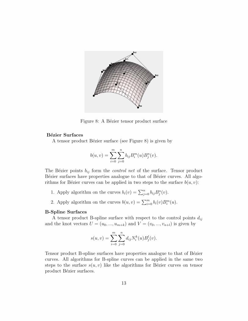
Figure 8: A Bezier tensor product surface

Bezier SurfacesA tensor product Bezier surface (see Figure 8) is given by

b(u, v) =m∑i=0

n∑j=0

bijBmi (u)Bn

j (v).

The Bezier points bij form the control net of the surface. Tensor productBezier surfaces have properties analogue to that of Bezier curves. All algo-rithms for Bezier curves can be applied in two steps to the surface b(u, v):

1. Apply algorithm on the curves bi(v) =∑n

j=0 bijBnj (v).

2. Apply algorithm on the curves b(u, v) =∑m

i=0 bi(v)Bmi (u).

B-Spline SurfacesA tensor product B-spline surface with respect to the control points dij

and the knot vectors U = (u0, ..., um+k) and V = (v0, ..., vn+l) is given by

s(u, v) =m∑i=0

n∑j=0

dijNki (u)Bl

j(v).

Tensor product B-spline surfaces have properties analogue to that of Beziercurves. All algorithms for B-spline curves can be applied in the same twosteps to the surface s(u, v) like the algorithms for Bezier curves on tensorproduct Bezier surfaces.

13

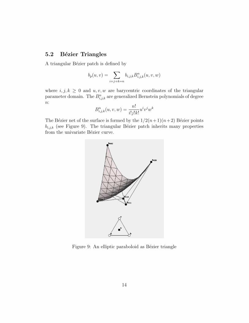
5.2 Bezier Triangles

A triangular Bezier patch is defined by

bp(u, v) =∑

i+j+k=n

bi,j,kBni,j,k(u, v, w)

where i, j, k ≥ 0 and u, v, w are barycentric coordinates of the triangularparameter domain. The Bn

i,j,k are generalized Bernstein polynomials of degreen:

Bni,j,k(u, v, w) =

n!

i!j!k!uivjwk

The Bezier net of the surface is formed by the 1/2(n+1)(n+2) Bezier pointsbi,j,k (see Figure 9). The triangular Bezier patch inherits many propertiesfrom the univariate Bezier curve.

Figure 9: An elliptic paraboloid as Bezier triangle

14

5.3 Algorithms

� The de Casteljau algorithm for triangular patches produces a tetrahe-dral scheme. The recursion formula for the computation is:

blijk = ubl−1i−1jk + vbl−1

ij−1k + wbl−1ijk−1

where i + j + k = n− l, (i, j, k ≥ 0) and b0ijk = bijk. It is easy to showthat bp(u, v, w) = bn000.

� Degree elevation

� Subdivision: the subdivision of the patch into three subpatches can bederived from the de Casteljau algorithm, like in the univariate case.

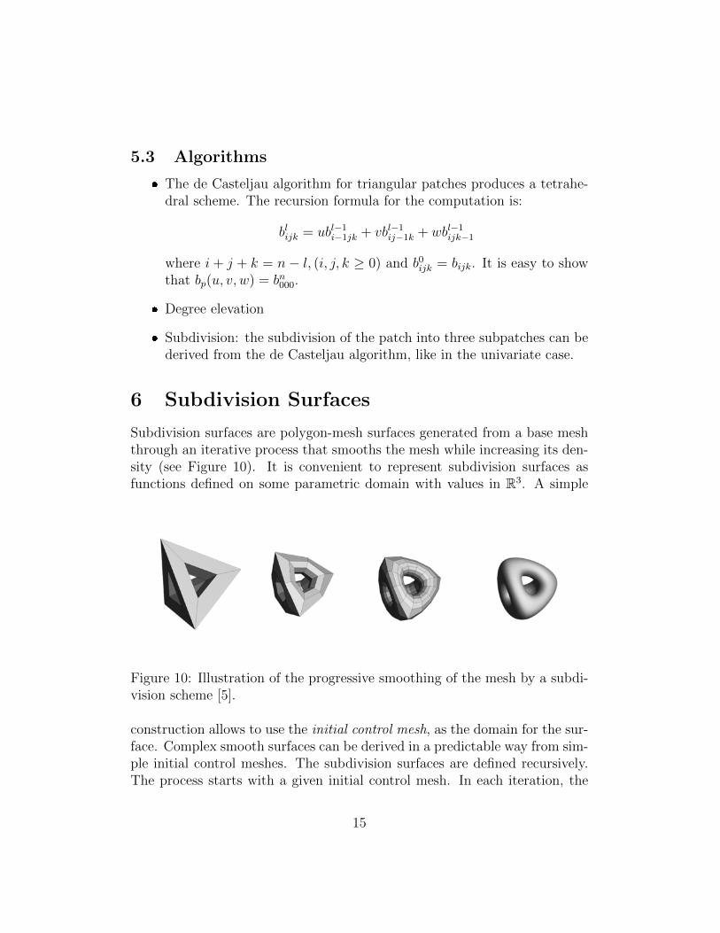
6 Subdivision Surfaces

Subdivision surfaces are polygon-mesh surfaces generated from a base meshthrough an iterative process that smooths the mesh while increasing its den-sity (see Figure 10). It is convenient to represent subdivision surfaces asfunctions defined on some parametric domain with values in R3. A simple

Figure 10: Illustration of the progressive smoothing of the mesh by a subdi-vision scheme [5].

construction allows to use the initial control mesh, as the domain for the sur-face. Complex smooth surfaces can be derived in a predictable way from sim-ple initial control meshes. The subdivision surfaces are defined recursively.The process starts with a given initial control mesh. In each iteration, the

15

subdivision process produces a increasing number of polygons [6]. The meshvertices converge to a limit surface through iteration step. Every subdivisionalgorithm has rules to calculate the locations of new vertices. Subdivisionrepresentations are suitable for many numerical simulation tasks which areof importance in engineering and computer animation.

A vertex v is a 3D position which describes the corners or intersectionsof geometric shapes. For example a triangle has three vertices. An edgeis a one-dimensional line segment connecting two adjacent zero-dimensionalvertices in a polygon. A planar closed sequence of edges forms a polygon(face). A polyhedron is a geometric solid in three dimensions with flat facesand straight edges. The valence of a vertex is the number of edges at thevertex. Subdivision rules are often specified by providing a mask. The maskis a visual scheme showing which vertices and weights are used to computea new vertex.

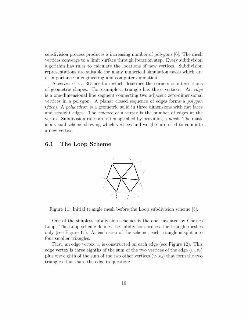
6.1 The Loop Scheme

Figure 11: Initial triangle mesh before the Loop subdivision scheme [5].

One of the simplest subdivision schemes is the one, invented by CharlesLoop. The Loop scheme defines the subdivision process for triangle meshesonly (see Figure 11). At each step of the scheme, each triangle is split intofour smaller triangles.

First, an edge vertex ve is constructed on each edge (see Figure 12). Thisedge vertex is three eighths of the sum of the two vertices of the edge (v1,v2)plus one eighth of the sum of the two other vertices (v3,v4) that form the twotriangles that share the edge in question:

16

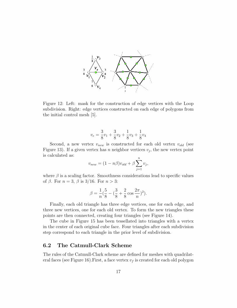
Figure 12: Left: mask for the construction of edge vertices with the Loopsubdivision. Right: edge vertices constructed on each edge of polygons fromthe initial control mesh [5].

ve =3

8v1 +

3

8v2 +

1

8v3 +

1

8v4

Second, a new vertex vnew is constructed for each old vertex vold (seeFigure 13). If a given vertex has n neighbor vertices vj, the new vertex pointis calculated as:

vnew = (1− nβ)vold + βn∑

j=1

vj,

where β is a scaling factor. Smoothness considerations lead to specific valuesof β. For n = 3, β is 3/16. For n > 3:

β =1

n(5

8− (

3

8+

2

8cos

2π

n)2).

Finally, each old triangle has three edge vertices, one for each edge, andthree new vertices, one for each old vertex. To form the new triangles thesepoints are then connected, creating four triangles (see Figure 14).

The cube in Figure 15 has been tessellated into triangles with a vertexin the center of each original cube face. Four triangles after each subdivisionstep correspond to each triangle in the prior level of subdivision.

6.2 The Catmull-Clark Scheme

The rules of the Catmull-Clark scheme are defined for meshes with quadrilat-eral faces (see Figure 16).First, a face vertex vf is created for each old polygon

17

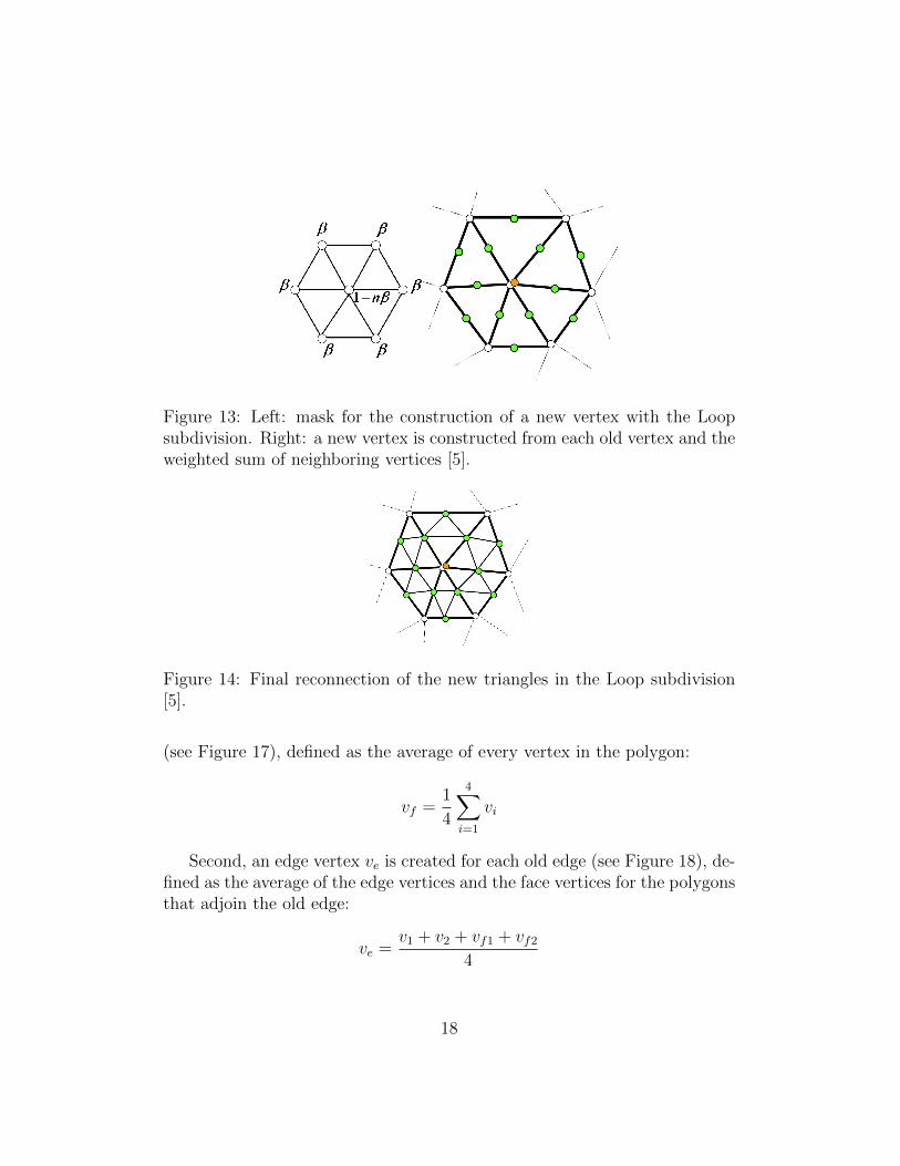
Figure 13: Left: mask for the construction of a new vertex with the Loopsubdivision. Right: a new vertex is constructed from each old vertex and theweighted sum of neighboring vertices [5].

Figure 14: Final reconnection of the new triangles in the Loop subdivision[5].

(see Figure 17), defined as the average of every vertex in the polygon:

vf =1

4

4∑i=1

vi

Second, an edge vertex ve is created for each old edge (see Figure 18), de-fined as the average of the edge vertices and the face vertices for the polygonsthat adjoin the old edge:

ve =v1 + v2 + vf1 + vf2

4

18

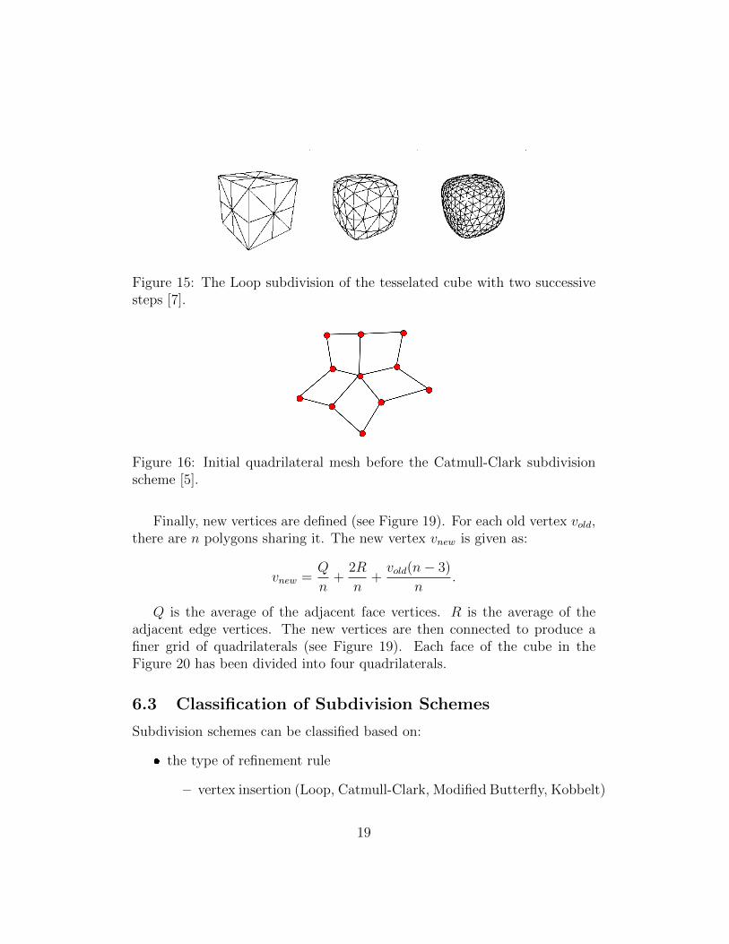
Figure 15: The Loop subdivision of the tesselated cube with two successivesteps [7].

Figure 16: Initial quadrilateral mesh before the Catmull-Clark subdivisionscheme [5].

Finally, new vertices are defined (see Figure 19). For each old vertex vold,there are n polygons sharing it. The new vertex vnew is given as:

vnew =Q

n+

2R

n+vold(n− 3)

n.

Q is the average of the adjacent face vertices. R is the average of theadjacent edge vertices. The new vertices are then connected to produce afiner grid of quadrilaterals (see Figure 19). Each face of the cube in theFigure 20 has been divided into four quadrilaterals.

6.3 Classification of Subdivision Schemes

Subdivision schemes can be classified based on:

� the type of refinement rule

– vertex insertion (Loop, Catmull-Clark, Modified Butterfly, Kobbelt)

19

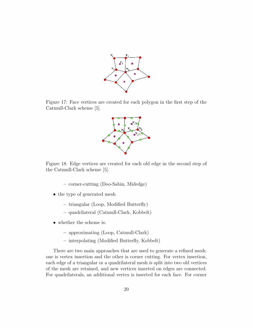
Figure 17: Face vertices are created for each polygon in the first step of theCatmull-Clark scheme [5].

Figure 18: Edge vertices are created for each old edge in the second step ofthe Catmull-Clark scheme [5].

– corner-cutting (Doo-Sabin, Midedge)

� the type of generated mesh

– triangular (Loop, Modified Butterfly)

– quadrilateral (Catmull-Clark, Kobbelt)

� whether the scheme is:

– approximating (Loop, Catmull-Clark)

– interpolating (Modified Butterfly, Kobbelt)

There are two main approaches that are used to generate a refined mesh:one is vertex insertion and the other is corner cutting. For vertex insertion,each edge of a triangular or a quadrilateral mesh is split into two old verticesof the mesh are retained, and new vertices inserted on edges are connected.For quadrilaterals, an additional vertex is inserted for each face. For corner

20

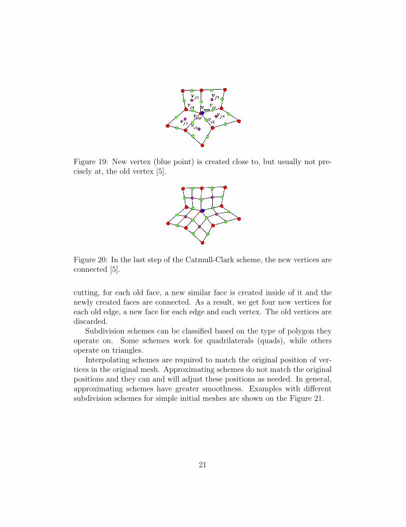
Figure 19: New vertex (blue point) is created close to, but usually not pre-cisely at, the old vertex [5].

Figure 20: In the last step of the Catmull-Clark scheme, the new vertices areconnected [5].

cutting, for each old face, a new similar face is created inside of it and thenewly created faces are connected. As a result, we get four new vertices foreach old edge, a new face for each edge and each vertex. The old vertices arediscarded.

Subdivision schemes can be classified based on the type of polygon theyoperate on. Some schemes work for quadrilaterals (quads), while othersoperate on triangles.

Interpolating schemes are required to match the original position of ver-tices in the original mesh. Approximating schemes do not match the originalpositions and they can and will adjust these positions as needed. In general,approximating schemes have greater smoothness. Examples with differentsubdivision schemes for simple initial meshes are shown on the Figure 21.

21

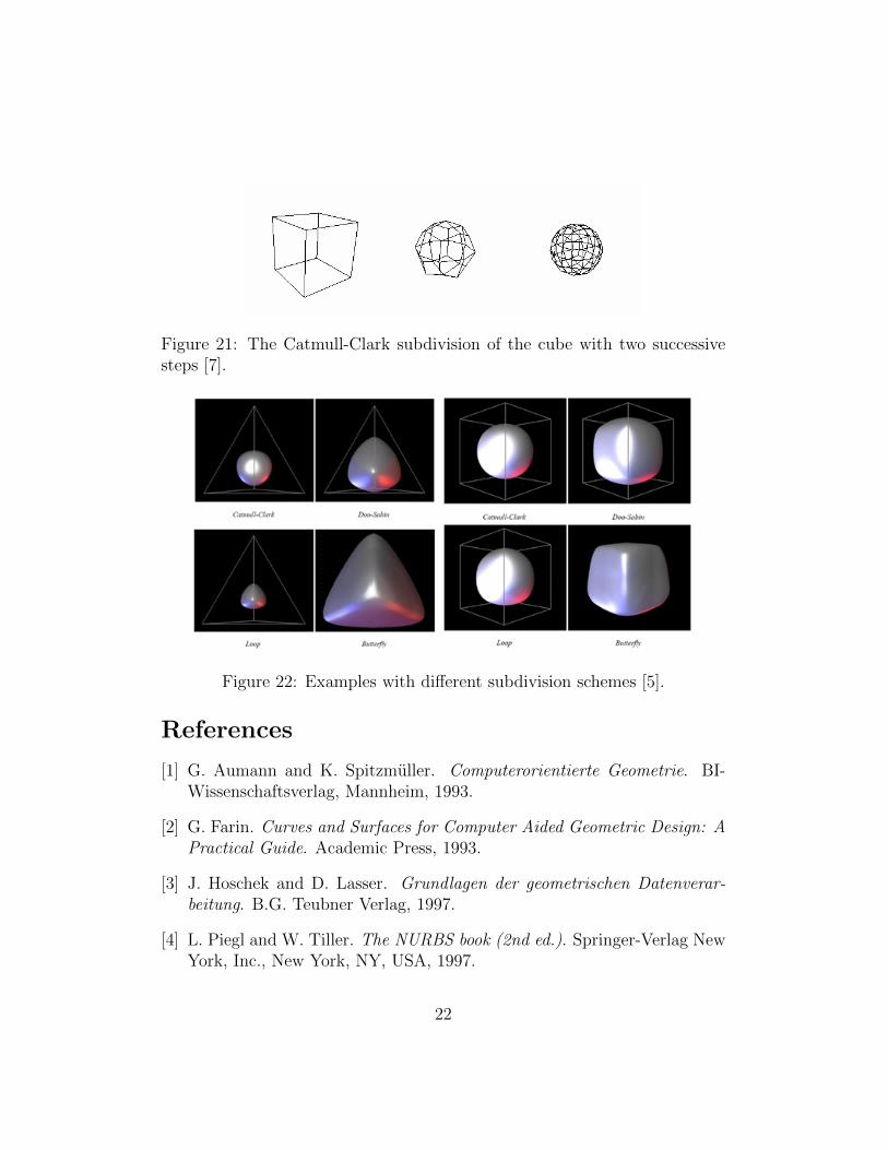
Figure 21: The Catmull-Clark subdivision of the cube with two successivesteps [7].

Figure 22: Examples with different subdivision schemes [5].

References

[1] G. Aumann and K. Spitzmuller. Computerorientierte Geometrie. BI-Wissenschaftsverlag, Mannheim, 1993.

[2] G. Farin. Curves and Surfaces for Computer Aided Geometric Design: APractical Guide. Academic Press, 1993.

[3] J. Hoschek and D. Lasser. Grundlagen der geometrischen Datenverar-beitung. B.G. Teubner Verlag, 1997.

[4] L. Piegl and W. Tiller. The NURBS book (2nd ed.). Springer-Verlag NewYork, Inc., New York, NY, USA, 1997.

22

[5] O. Weber. Subdivision Surfaces. http://www.cs.technion.ac.il/

~cs236716/, 2011. [Online; accessed 04-March-2011].

[6] D. Zorin, P. Schroder, T. Derose, L. Kobbelt, A. Levin, and W. Sweldens.Subdivision for Modeling and Animation. In SIGGRAPH Course Notes,New York, 2000. ACM.

[7] R. Holmes. A Quick Introduction to Subdivision Surfaces. http://

www.holmes3d.net/graphics/subdivision/, 2011. [Online; accessed04-March-2011].

23