Advances in the geotechnical characterization of Mexico City basin subsoil Juárez Moisés, Auvinet Gabriel & Méndez Edgar, Instituto de Ingeniería, UNAM, Mexico, D.F., Mexico Rodríguez Martha & Barranco Alejandro Instituto de Ingeniería, UNAM, Mexico, D.F., Mexico ABSTRACT This paper presents recent advances in the geotechnical characterization of Mexico City subsoil based on a Geographic Information System for Geotechnical Borings (GIS-GB) that includes more than 7,000 soil profiles. Geostatistical techniques were used to define 2D and 3D models of the subsoil. Contours map of layers thickness, as well as index (water content) and mechanical (CPT point resistance) properties in the area were also obtained. The maps that have been established have been used in order to update the geotechnical zoning presented in Mexico City Building Code. RESUMEN En este trabajo se presenta una contribución a la caracterización del subsuelo de origen lacustre de la zona norte de la cuenca de México, a partir de los resultados de exploraciones geotécnicas. Se emplea la Geoestadística como herramienta para definir modelos 2D y 3D del subsuelo. Se han obtenido mapas de isovalores de espesores de estratos y de propiedades índice (contenido de agua) y mecánicas (resistencia de punta en pruebas de cono) para el área de estudio. Los mapas que se han construido se han usado para actualizar la zonificación geotécnica del Reglamento de Construcciones de la Ciudad de México. 1 INTRODUCTION The numerous geotechnical borings performed in the urban area of Mexico City can be used to obtain a better knowledge of the subsoil and improve the accuracy of geotechnical zoning maps for regulatory purposes of construction (GDF, 2004).

To take advantage of the new available information, it has been considered as necessary to use computational and informatics tools, such as Geographical Information Systems as well as powerful mathematical tools based on Geostatistics.

Geographic Information Systems help to organize geotechnical information for fast and easy review. On the other hand, Geostatistics, defined as the application of random functions theory to the description of the spatial distribution of properties of geological materials, provides valuable tools for estimating data such as thickness of a specific stratum, or value of a certain soil property at a given point where no information is available, taking into account the correlation structure of the medium. Additionally, uncertainty associated to these estimations can be quantified.

Fundamentals of Geostatistics applied to Geotechnics have been presented in detail in some previous publications and contributions to different conferences (Auvinet, 2002; Juárez and Auvinet, 2002). This paper illustrates the direct application of geostatistical methods to the assessment of spatial variations of soil properties (water content and CPT point resistance) and geometric configuration of layers (depth and thickness) in the lacustrine zone of Mexico City.

In previous papers the geotechnical characterization subsoil for some areas of Mexico City has been presented. In 2009, the west zone and downtown area were described (Auvinet, 2009). This paper deals with the subsoil geotechnical characterization of the east and south zones of Mexico City. 2 LOCATION OF STUDY AREA The study area is located to the east of Mexico City. It includes parts of municipalities of Tlalnepantla, Texcoco and Nezahualcoyotl in the State of Mexico and the area named “Federal zone of Texcoco Lake” (Figure 1).

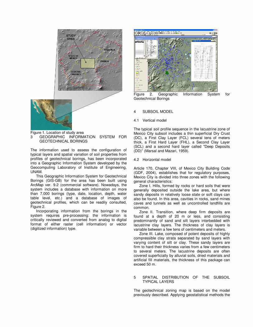
Figure 1. Location of study area 3 GEOGRAPHIC INFORMATION SYSTEM FOR

GEOTECHNICAL BORINGS The information used to assess the configuration of typical layers and spatial variation of soil properties from profiles of geotechnical borings, has been incorporated into a Geographic Information System developed by the Geocomputing Laboratory of Institute of Engineering, UNAM.

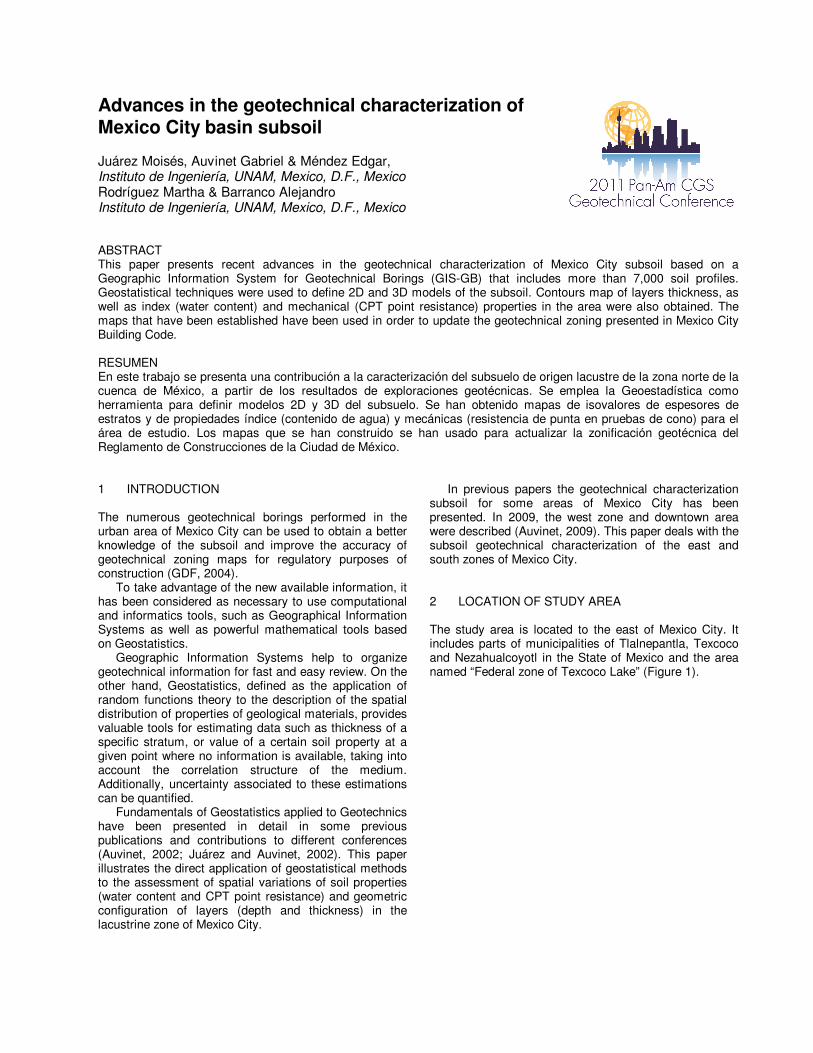
This Geographic Information System for Geotechnical Borings (GIS-GB) for the area has been built using ArcMap ver. 9.2 (commercial software). Nowadays, the system includes a database with information on more than 7,000 borings (type, date, location, depth, water table level, etc.) and a database of images of geotechnical profiles, which can be readily consulted, Figure 2.

Incorporating information from the borings in the system requires pre-processing: the information is critically reviewed and converted from analog to digital format of either raster (cell information) or vector (digitized information) type.

Figure 2. Geographic Information System for Geotechnical Borings 4 SUBSOIL MODEL 4.1 Vertical model The typical soil profile sequence in the lacustrine zone of Mexico City subsoil includes a thin superficial Dry Crust (DC), a First Clay Layer (FCL) several tens of meters thick, a First Hard Layer (FHL), a Second Clay Layer (SCL) and a second hard layer called "Deep Deposits (DD)” (Marsal and Mazari, 1959). 4.2 Horizontal model Article 170, Chapter VIII, of Mexico City Building Code (GDF, 2004), establishes that for regulatory purposes, Mexico City is divided into three zones with the following general characteristics:

Zone I. Hills, formed by rocks or hard soils that were generally deposited outside the lake area, but where sandy deposits in relatively loose state or soft clays can also be found. In this area, cavities in rocks, sand mines caves and tunnels as well as uncontrolled landfills are common.

Zone II. Transition, where deep firm deposits are found at a depth of 20 m or less, and consisting predominantly of sand and silt layers interbedded with lacustrine clay layers. The thickness of clay layers is variable between a few tens of centimeters and meters.

Zone III. Lake, composed of potent deposits of highly compressible clay strata separated by sand layers with varying content of silt or clay. These sandy layers are firm to hard their thickness varies from a few centimeters to several meters. The lacustrine deposits are often covered superficially by alluvial soils, dried materials and artificial fill materials, the thickness of this package can exceed 50 m. 5 SPATIAL DISTRIBUTION OF THE SUBSOIL

TYPICAL LAYERS

The geotechnical zoning map is based on the model previously described. Applying geostatistical methods the

depth of deep deposits (FCL) is considered as a random field V(X), distributed within an R

P domain, with p = 2 (area). The set of measured values within the RP domain is a sample of this random field. After removing a linear trend, a structural analysis was performed to obtain experimental correlograms (Figure 3) and to asess correlation distances (δ0°= 450m and (δ90°= 430m). The theoretical correlograms were fitted to an exponential equation taking into account the corresponding correlation distances (Figure 3).

-0.4

-0.2

0

0.2

0.4

0.6

0.8

1

0 500 1000 1500 2000 2500 3000 3500Cor

rela

tion

coe

ffic

ient

, ρ

Distance, h(m)

Experimental correlogram

Exponential correlogram

a) Correlogram for direction Az =0°

-0.6

-0.4

-0.2

0

0.2

0.4

0.6

0.8

1

0 500 1000 1500 2000 2500 3000 3500

Co

rrel

atio

n c

oeff

icie

nt,

ρ

Distance, h(m)

Experimental correlogram

Exponential correlogram

b) Correlogram for direction Az =90°

Figure 3. Directional correlograms for FCL depth From the data set without trend (residual field) and

using the results of structural analysis, the expected value and standard deviation of the depth of the FCL were obtained for all nodes of a regular grid conveniently defined, using the technique of Ordinary Kriging (Journel & Deutch 1992). The final estimate of the field was obtained reinstating the trend into the results. A contour map could then be drawn, Figure 4.

CHICOLOAPAN

BOSQUE

SAN JUAN

AV. EDUARDO M

OLINA

COATLINCHAN

NEZAHUALCOYOTL

TEZOYUCA

CHICONCUACPAPALOTLA

ECATEPEC DE MORELOS

SANTACLARA

SAN MIGUEL

TOCUILA

A MEXICO

AV. CENTRAL

VASO DEL LAGO DE TEXCOCO

C. CHIMALHUACAN

DE ARAGON

Laguna

flacultativa

Lago Nabor

Carrillo

Lago

Churubusco

Lago

regulación

horaria

Laguna

Casa

Colorada

TEXCOCO

TLALNEPANTLA

CHIAUTLA

SAN SALVADOR

ATENCO

CIUDAD

AZTECA

MONTECILLO

SIERRA NEVADA

LAS AMERICAS

SIERRA DE GUADALUPE

-0.5

-1.5

-1.0

- 2.0

-2.5

-3.0

-3. 5

-4.0

-4.5

-2.5

-2.5

-0

.5

-1.0

-1.5

-4.0-3.5

-2.0

-2.0

-2.5

-3.0

- 4.0

-1.0

-1.0

-1.5

-1 .0

-3.5

- 0.5

-2.5

-3.5

- 3.0

-1.5-0.5

- 2.0

-2.5

-3.0

-0.5

-0.5

-3.5

-1.5

-1.0

-2.5

-1.0

-0.5

-3.5

-0.5

-3.0

-1.0

-3.0

-2.0

-3.5

- 1.5

-2.0

-0.5

-4 .5-2 .0

-1. 0

-2.0

-2.5

-1.0

-1.0

-2.5

-2.5

-1.0

-2.0

-2 .5

-2.0

-2.5

-2.5

-3.5-3 .5

488305 494120 499935 505750 511565 517380

214

497

521

505

102

156

045

2161

580

8A

1'

2'

3'

4'

5'

B C D

A' B' C' D'

1

2

3

4

5

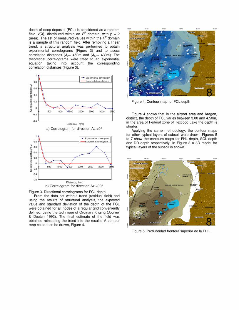
Figure 4. Contour map for FCL depth Figure 4 shows that in the airport area and Aragon,

district, the depth of FCL varies between 3.00 and 4.50m, in the area of Federal zone of Texcoco Lake the depth is shorter.

Applying the same methodology, the contour maps for other typical layers of subsoil were drawn. Figures 5 to 7 show the contours maps for FHL depth, SCL depth and DD depth respectively. In Figure 8 a 3D model for typical layers of the subsoil is shown.

CHICOLOAPAN

BOSQUE

SAN JUAN

AV. EDUARDO M

OLINA

COATLINCHAN

NEZAHUALCOYOTL

TEZOYUCA

CHICONCUACPAPALOTLA

ECATEPEC DE MORELOS

SANTA

CLARA

SAN MIGUEL

TOCUILA

A MEXICO

AV. CENTRAL

VASO DEL LAGO DE TEXCOCO

C. CHIMALHUACAN

DE ARAGON

Laguna

flacultativa

Lago Nabor

Carrillo

Lago

Churubusco

Lago

regulación

horaria

Laguna

Casa

Colorada

TEXCOCO

TLALNEPANTLA

CHIAUTLA

SAN SALVADOR

ATENCO

CIUDAD

AZTECA

MONTECILLO

SIERRA NEVADA

LAS AMERICAS

SIERRA DE GUADALUPE

- 20.

0

-25.0

-35.0

-30.0

-40.

0

-45.0

-25.

0

-20.

0

-25.0

-20.0

-20.0

-30.0

-30. 0

488305 494120 499935 505750 511565 517380

214

497

52

150

510

215

604

52

161

580

8A

1'

2'

3'

4'

5'

B C D

A' B' C' D'

1

2

3

4

5

Figure 5. Profundidad frontera superior de la FHL

CHICOLOAPAN

BOSQUE

SAN JUAN

AV. EDUARDO M

OLINA

COATLINCHAN

NEZAHUALCOYOTL

TEZOYUCA

CHICONCUACPAPALOTLA

ECATEPEC DE MORELOS

SANTA

CLARA

SAN MIGUEL

TOCUILA

A MEXICO

AV. CENTRAL

VASO DEL LAGO DE TEXCOCO

C. CHIMALHUACAN

DE ARAGON

Laguna

flacultativa

Lago Nabor

Carrillo

Lago

Churubusco

Lago

regulación

horaria

Laguna

Casa

Colorada

TEXCOCO

TLALNEPANTLA

CHIAUTLA

SAN SALVADOR

ATENCO

CIUDAD

AZTECA

MONTECILLO

SIERRA NEVADA

LAS AMERICAS

SIERRA DE GUADALUPE

-20 .

0

-25.0

-35.0

-40.0

-30.0

-20.

0

- 25. 0

-25.0

-20.0

-35.

0

-20.0

-30

.0

-30.0

488305 494120 499935 505750 511565 5173802

144

975

215

051

021

560

45

216

158

0

8A

1'

2'

3'

4'

5'

B C D

A' B' C' D'

1

2

3

4

5

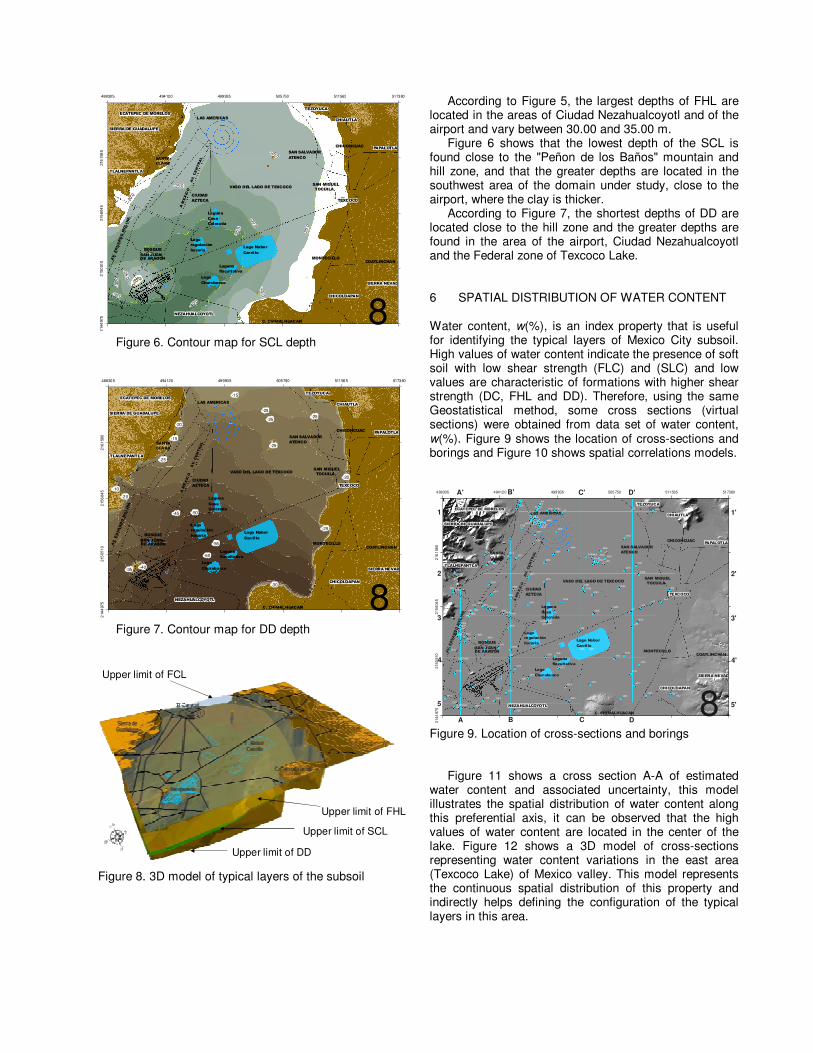
Figure 6. Contour map for SCL depth

CHICOLOAPAN

BOSQUE

SAN JUAN

AV. EDUARDO M

OLINA

COATLINCHAN

NEZAHUALCOYOTL

TEZOYUCA

CHICONCUACPAPALOTLA

ECATEPEC DE MORELOS

SANTA

CLARA

SAN MIGUEL

TOCUILA

A MEXICO

AV. CENTRAL

VASO DEL LAGO DE TEXCOCO

C. CHIMALHUACAN

DE ARAGON

Laguna

flacultativa

Lago Nabor

Carrillo

Lago

Churubusco

Lago

regulación

horaria

Laguna

Casa

Colorada

TEXCOCO

TLALNEPANTLA

CHIAUTLA

SAN SALVADOR

ATENCO

CIUDAD

AZTECA

MONTECILLO

SIERRA NEVADA

LAS AMERICAS

SIERRA DE GUADALUPE

-45

-40-35

-50

-55

-60

-25

-20

-15

-10

-30

-25-25

-25

-20

-20

-25

-25

-15

488305 494120 499935 505750 511565 517380

214

497

521

505

102

156

045

2161

580

8A

1'

2'

3'

4'

5'

B C D

A' B' C' D'

1

2

3

4

5

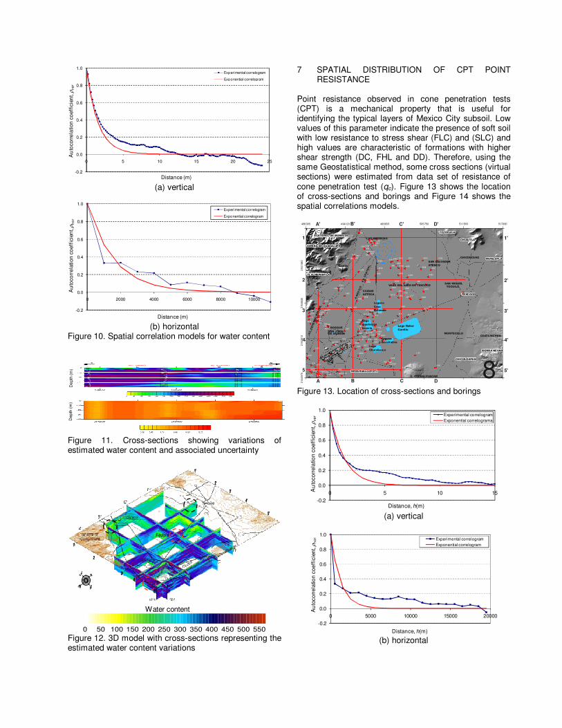
Figure 7. Contour map for DD depth

Upper limit of FCL

Upper limit of FHL

Upper limit of SCL

Upper limit of DD

Figure 8. 3D model of typical layers of the subsoil

According to Figure 5, the largest depths of FHL are located in the areas of Ciudad Nezahualcoyotl and of the airport and vary between 30.00 and 35.00 m.

Figure 6 shows that the lowest depth of the SCL is found close to the "Peñon de los Baños" mountain and hill zone, and that the greater depths are located in the southwest area of the domain under study, close to the airport, where the clay is thicker.

According to Figure 7, the shortest depths of DD are located close to the hill zone and the greater depths are found in the area of the airport, Ciudad Nezahualcoyotl and the Federal zone of Texcoco Lake. 6 SPATIAL DISTRIBUTION OF WATER CONTENT Water content, w(%), is an index property that is useful for identifying the typical layers of Mexico City subsoil. High values of water content indicate the presence of soft soil with low shear strength (FLC) and (SLC) and low values are characteristic of formations with higher shear strength (DC, FHL and DD). Therefore, using the same Geostatistical method, some cross sections (virtual sections) were obtained from data set of water content, w(%). Figure 9 shows the location of cross-sections and borings and Figure 10 shows spatial correlations models.

CHICOLOAPAN

BOSQUE

SAN JUAN

AV. EDUARDO M

OLINA

COATLINCHAN

NEZAHUALCOYOTL

TEZOYUCA

CHICONCUACPAPALOTLA

ECATEPEC DE MORELOS

SANTA

CLARA

SAN MIGUEL

TOCUILA

A MEXICO

AV. CENTRAL

VASO DEL LAGO DE TEXCOCO

C. CHIMALHUACAN

DE ARAGON

Laguna

flacultativa

Lago Nabor

Carrillo

Lago

Churubusco

Lago

regulación

horaria

Laguna

Casa

Colorada

TEXCOCO

TLALNEPANTLA

CHIAUTLA

SAN SALVADOR

ATENCO

CIUDAD

AZTECA

MONTECILLO

SIERRA NEVADA

LAS AMERICAS

SIERRA DE GUADALUPE

321

474645

4443

4241

39

38

3736

3532

3130

28

2120

1917

13

924

541

415

414

413

408

401

135

5066

5060

50595058

5057

50195017

4498

4496

4495

4494

4493

44924491

44904489

4485

4470

4469

4468

4460

4447

4446

4445

4443

4442

44414440

4439

44384437

44364435

44344433

44324431

4430

4429

4428

42134137

41104101

4097

4094

4090

4089

4086

4085

4084 4077

4076

4075

40744073

4071

4070

4068

4065

4064

4063

4062

4059

4054

4053

4052

4038 4035

3905

3881

3810

3657

3639

3597

3571

3563

3562

3545

3535

3521

3518

3514

3512

3490

3489

3480

3474

3456

3454

3452

3451

3446

3445

3441

34383437

3436

3431

3430

3429

239223912370

2367 2365

2195

2193

1963

1961

1935

1855

17831782

16321626

488305 494120 499935 505750 511565 517380

2144

975

2150

510

215

6045

216

1580

8A B C D

A' B' C' D'

5

4

3

2

1

5'

4'

3'

2'

1'

Figure 9. Location of cross-sections and borings

Figure 11 shows a cross section A-A of estimated water content and associated uncertainty, this model illustrates the spatial distribution of water content along this preferential axis, it can be observed that the high values of water content are located in the center of the lake. Figure 12 shows a 3D model of cross-sections representing water content variations in the east area (Texcoco Lake) of Mexico valley. This model represents the continuous spatial distribution of this property and indirectly helps defining the configuration of the typical layers in this area.

-0.2

0.0

0.2

0.4

0.6

0.8

1.0

0 5 10 15 20 25

Au

toco

rre

latio

n c

oef

ficie

nt,

ρver

Distance (m)

Experimental correlogram

Exponential correlogram

(a) vertical

-0.2

0.0

0.2

0.4

0.6

0.8

1.0

0 2000 4000 6000 8000 10000

Au

toco

rrel

atio

n c

oeff

icie

nt,ρ

ho

r

Distance (m)

Experimental correlogram

Exponential correlogram

(b) horizontal

Figure 10. Spatial correlation models for water content

De

pth

(m)

De

pth

(m)

Figure 11. Cross-sections showing variations of estimated water content and associated uncertainty

0 50 100 150 200 250 300 350 400 450 500 550 Figure 12. 3D model with cross-sections representing the estimated water content variations

7 SPATIAL DISTRIBUTION OF CPT POINT RESISTANCE

Point resistance observed in cone penetration tests (CPT) is a mechanical property that is useful for identifying the typical layers of Mexico City subsoil. Low values of this parameter indicate the presence of soft soil with low resistance to stress shear (FLC) and (SLC) and high values are characteristic of formations with higher shear strength (DC, FHL and DD). Therefore, using the same Geostatistical method, some cross sections (virtual sections) were estimated from data set of resistance of cone penetration test (qc). Figure 13 shows the location of cross-sections and borings and Figure 14 shows the spatial correlations models.

CHICOLOAPAN

BOSQUE

SAN JUAN

AV. EDUARDO M

OLINA

COATLINCHAN

NEZAHUALCOYOTL

TEZOYUCA

CHICONCUACPAPALOTLA

ECATEPEC DE MORELOS

SANTACLARA

SAN MIGUELTOCUILA

A MEXICO

AV. CENTRAL

VASO DEL LAGO DE TEXCOCO

C. CHIMALHUACAN

DE ARAGON

Laguna

flacultativa

Lago Nabor

Carrillo

Lago

Churubusco

Lago

regulación

horar ia

Laguna

Casa

Colorada

TEXCOCO

TLALNEPANTLA

CHIAUTLA

SAN SALVADOR

ATENCO

CIUDAD

AZTECA

MONTECILLO

SIERRA NEVADA

LAS AMERICAS

SIERRA DE GUADALUPE

321

3332

922921920

916

686

685

644

641640

610

60 2

540

530529

502501500

420

41 9

418

417

412

410409

407406

404402

360359239238

188187

114113

5061

5040

500250015000

4503

4502 4501 4500 4499

4497

4488

448744 8644854484

448344824481

44644463

44624461

44594452

4451

44274406

4223

4210

42 09

41 61

3990

3949

3948

3931

39253924

3825

365636553654

3653

3650

2579

2374

20232012

2003

1962

1936

1934

1930

1929192819271926

1925

19231917

16671666

16641663

16 56

1651

1650

1649

1643

1642

1640

1639

1638

16211619

1618

1616

1615

1614

1611

1608

1607

1606

16051604

1603

1602

1599

1598

1597

1595 1592

15911590

1587

1583

1582

1581

1580

15 791575

1465

1454

138313821381

13 80 13721368

118911 88

1187

1181

10501049

488305 494120 499935 505750 511565 517380

2144

975

215

0510

215

6045

2161

580

8A B C D

A' B' C' D'

5

4

3

2

1

5'

4'

3'

2'

1'

Figure 13. Location of cross-sections and borings

-0.2

0.0

0.2

0.4

0.6

0.8

1.0

0 5 10 15Au

toco

rrel

atio

n c

oeff

icie

nt,ρ

ve

r

Distance, h(m)

Experimental correlogramExponential correlograma

(a) vertical

-0.2

0.0

0.2

0.4

0.6

0.8

1.0

0 5000 10000 15000 20000

Au

toco

rrel

atio

n c

oeff

icie

nt,ρ

ho

r

Distance, h(m)

Experimental correlogramExponential correlogram

(b) horizontal

Water content

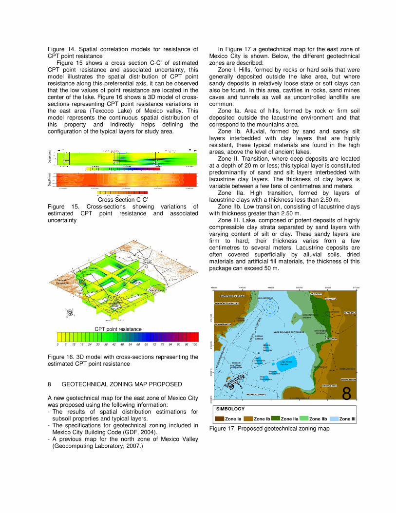
Figure 14. Spatial correlation models for resistance of CPT point resistance

Figure 15 shows a cross section C-C’ of estimated CPT point resistance and associated uncertainty, this model illustrates the spatial distribution of CPT point resistance along this preferential axis, it can be observed that the low values of point resistance are located in the center of the lake. Figure 16 shows a 3D model of cross-sections representing CPT point resistance variations in the east area (Texcoco Lake) of Mexico valley. This model represents the continuous spatial distribution of this property and indirectly helps defining the configuration of the typical layers for study area.

Dep

th(m

)

2146000 2151000 2156000 2161000 2166000

-40

-30

-20

-10

0

De

pth

(m)

Cross Section C-C’

Figure 15. Cross-sections showing variations of estimated CPT point resistance and associated uncertainty

0 6 12 18 24 30 36 42 48 54 60 66 72 78 84 90 96 100

Figure 16. 3D model with cross-sections representing the estimated CPT point resistance 8 GEOTECHNICAL ZONING MAP PROPOSED A new geotechnical map for the east zone of Mexico City was proposed using the following information: - The results of spatial distribution estimations for

subsoil properties and typical layers. - The specifications for geotechnical zoning included in

Mexico City Building Code (GDF, 2004). - A previous map for the north zone of Mexico Valley

(Geocomputing Laboratory, 2007.)

In Figure 17 a geotechnical map for the east zone of Mexico City is shown. Below, the different geotechnical zones are described:

Zone I. Hills, formed by rocks or hard soils that were generally deposited outside the lake area, but where sandy deposits in relatively loose state or soft clays can also be found. In this area, cavities in rocks, sand mines caves and tunnels as well as uncontrolled landfills are common.

Zone Ia. Area of hills, formed by rock or firm soil deposited outside the lacustrine environment and that correspond to the mountains area.

Zone Ib. Alluvial, formed by sand and sandy silt layers interbedded with clay layers that are highly resistant, these typical materials are found in the high areas, above the level of ancient lakes.

Zone II. Transition, where deep deposits are located at a depth of 20 m or less; this typical layer is constituted predominantly of sand and silt layers interbedded with lacustrine clay layers. The thickness of clay layers is variable between a few tens of centimetres and meters.

Zone IIa. High transition, formed by layers of lacustrine clays with a thickness less than 2.50 m.

Zone IIb. Low transition, consisting of lacustrine clays with thickness greater than 2.50 m.

Zone III. Lake, composed of potent deposits of highly compressible clay strata separated by sand layers with varying content of silt or clay. These sandy layers are firm to hard; their thickness varies from a few centimetres to several meters. Lacustrine deposits are often covered superficially by alluvial soils, dried materials and artificial fill materials, the thickness of this package can exceed 50 m.

CHICOLOAPAN

BOSQUE

SAN JUAN

AV. EDUARDO MOLINA

COATLINCHAN

NEZAHUALCOYOTL

TEZOYUCA

CHICONCUACPAPALOTLA

ECATEPEC DE MORELOS

SANTA

CLARA

SAN MIGUEL

TOCUILA

A MEXICO

AV. CENTRAL

VASO DEL LAGO DE TEXCOCO

C. CHIMALHUACAN

DE ARAGON

Laguna

flacultativa

Lago Nabor

Carrillo

Lago

Churubusco

Lago

regulación

horaria

Laguna

Casa

Colorada

TEXCOCO

TLALNEPANTLA

CHIAUTLA

SAN SALVADOR

ATENCO

CIUDAD

AZTECA

MONTECILLO

SIERRA NEVADA

LAS AMERICAS

SIERRA DE GUADALUPE

488305 494120 499935 505750 511565 517380

2144

975

2150

510

2156

045

2161

580

8

SIMBOLOGY

Zone Ia Zone Ib Zone IIa Zone IIb Zone III

Figure 17. Proposed geotechnical zoning map

CPT point resistance

9 APPLICATION TO A NEW LINEAR INFRASTRUCTURE WORK OF THE TRANSPORT SYSTEM

To illustrate the applicability of the results of this research, the analyses for the water content and CPT point resistance of the subsoil along the proposed route to be followed by a new linear infrastructure work of the transport system are presented.

The new linear infrastructure work is located south of Mexico City, it is approximately 25 km long. The axis of the project crosses several political precincts: Benito Juárez, Álvaro Obregón, Coyoacán, Iztapalapa y Tláhuac (Figure 18).

Project axis

Figure 18. Location of a new linear infrastructure work

Most of the project is located in lacustrine soil but

several other types of geological materials are found (Figure 19).

Project axis

Figure 19. Geology (Mooser, 1996)

The geotechnical characterization of subsoil along the

project axis was made applying the previously exposed geostatistical method.

Figure 20 shows the location of borings used for the geostatistics analysis for water content w(%) and Figure 21 shows the location of borings used for the geostatistics analysis for CPT point resistance.

Project axis

Figure 20. Location of borings used for geostatistical analysis for water content, w(%)

Project axis

Figure 21. Location of borings used for geostatistical analysis for CPT point resistance

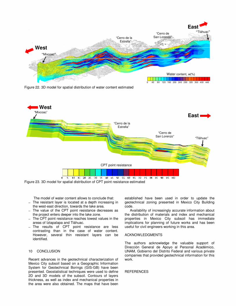
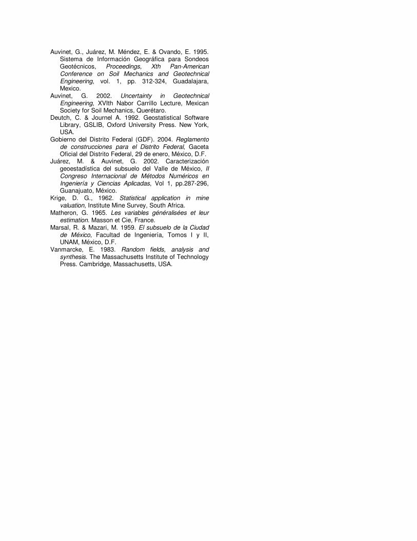
In Figures 22 and 23, a 3D model for the water content and CPT point resistance are shown respectively, these models can be updated easily when additional information becomes available.

The water content model permits to observe that: − To the west, the low water content corresponds to the

hill zone. − The highest water contents are found in the lake zone.

Within the clay formation, some substrates with different water content can be observed whose configuration is random but presents some degree of horizontal continuity.

− Close to “Cerro de la Estrella” and “Cerro de San Lorenzo” the water content decreases.

− The water content is more uniform in the areas of Chalco and Tláhuac lakes.

Water content, w(%)

“Cerro de la Estrella”

“Cerro de San Lorenzo”

West

East

“Mixcoac”

“Tláhuac”

Figure 22. 3D model for spatial distribution of water content estimated

CPT point resistance

“Cerro de la Estrella”

“Cerro de San Lorenzo”

West

East“Mixcoac”

“Tláhuac”

Figure 23. 3D model for spatial distribution of CPT point resistance estimated

The model of water content allows to conclude that: − The resistant layer is located at a depth increasing in

the west-east direction, towards the lake area. − The value of the CPT point resistance decreases as

the project enters deeper into the lake zone. − The CPT point resistance reaches lowest values in the

areas of Iztapalapa and Tláhuac. − The results of CPT point resistance are less

contrasting than in the case of water content. However, several thin resistant layers can be identified.

10 CONCLUSION Recent advances in the geotechnical characterization of Mexico City subsoil based on a Geographic Information System for Geotechnical Borings (GIS-GB) have been presented. Geostatistical techniques were used to define 2D and 3D models of the subsoil. Contours of layers thickness, as well as index and mechanical properties in the area were also obtained. The maps that have been

established have been used in order to update the geotechnical zoning presented in Mexico City Building code.

Availability of increasingly accurate information about the distribution of materials and index and mechanical properties in Mexico City subsoil has immediate implications for planning of future works and has been useful for civil engineers working in this area. ACKNOWLEDGMENTS The authors acknowledge the valuable support of Dirección General de Apoyo al Personal Académico, UNAM, Gobierno del Distrito Federal and various private companies that provided geotechnical information for this work. REFERENCES

Auvinet, G., Juárez, M. Méndez, E. & Ovando, E. 1995. Sistema de Información Geográfica para Sondeos Geotécnicos, Proceedings, Xth Pan-American Conference on Soil Mechanics and Geotechnical Engineering, vol. 1, pp. 312-324, Guadalajara, Mexico.

Auvinet, G. 2002. Uncertainty in Geotechnical Engineering, XVIth Nabor Carrillo Lecture, Mexican Society for Soil Mechanics, Querétaro.

Deutch, C. & Journel A. 1992. Geostatistical Software Library, GSLIB, Oxford University Press. New York, USA.

Gobierno del Distrito Federal (GDF). 2004. Reglamento de construcciones para el Distrito Federal, Gaceta Oficial del Distrito Federal, 29 de enero, México, D.F.

Juárez, M. & Auvinet, G. 2002. Caracterización geoestadística del subsuelo del Valle de México, II Congreso Internacional de Métodos Numéricos en Ingeniería y Ciencias Aplicadas, Vol 1, pp.287-296, Guanajuato, México.

Krige, D. G., 1962. Statistical application in mine valuation, Institute Mine Survey, South Africa.

Matheron, G. 1965. Les variables généralisées et leur estimation. Masson et Cie, France.

Marsal, R. & Mazari, M. 1959. El subsuelo de la Ciudad de México, Facultad de Ingeniería, Tomos I y II, UNAM, México, D.F.

Vanmarcke, E. 1983. Random fields, analysis and synthesis. The Massachusetts Institute of Technology Press. Cambridge, Massachusetts, USA.