Embed Size (px)
Citation preview

* Corresponding Author
Received: 08 April 2017 Accepted: 06 June 2017
Adıyaman University Journal of Science
dergipark.gov.tr/adyusci
ADYUSCI
7 (1) (2017) 60-88
Interval Linear Programming And Fuzzy DEA-BCC Models With Ranking Of
DMU New Approach
Oday JARJIES1,*, Hasan BAL2
1Mosul University, Faculty of Computer Science and Mathematics, Department of Operations Research
and Technology Intelligence, Mosul, Iraq, [email protected]
2Gazi University, Faculty of Sciences, Department of Statistics, 06500 Ankara, Türkiye,
Abstract
In this paper, a new approach for obtaining Ranking efficiency with the fuzzy
data numbers are being considered. Most Fuzzy DEA models are introduced in the
literatary words which are parametric models structured on alpha cuts. yet , the model
is introduced in this study is parametric and is used trapezoidal fuzzy number. From the
theotrical perspective, the objective of this study is to develop a simple and effective
Fuzzy DEA-BCC model. The most and maximum possible efficiency scores of each
DMU are estimated a few α-level, this model can be applied to determine many issues
are associated with qualitative factors. It is checked by applying the proposed method
in two numerical examples are compared with the results of eight current models of
fuzzy DEA.
Keywords: Fuzzy DEA, Efficiency Measurement, Ranking Model, α-Level,
Decision Making Unit.

61
Aralıklı Lineer Programlama ve Bulanık VZA-BCC Modelleri ile KVB
Sıralamalı Yeni Yaklaşım
Özet
Bu yazıda, bulanık veri sayıları ile Sıralamada etkinlik elde etmek için yeni bir
yaklaşım ele alınmaktadır.Literatürde sunulan bulanık KVB modellerinin çoğu, alfa kesimler
üzerinde yapılandırılmış parametrik modellerdir.Ancak bu çalışmada tanıtılan model
parametriktir ve trapezoid bulanık sayı kullanmaktadır. Teori perspektifinden, bu çalışmanın
amacı, basit ve etkili bir Bulanık KVB-BCC modeli geliştirmektir. Her bir KVB'nun mümkün
olan en fazla ve en fazla verim puanının birkaç α seviyesinde olduğu tahmin edilmektedir, bu
model, nitel faktörlerle ilişkili birçok sorunu belirlemek için uygulanabilir.İki sayısal örnekte
önerilen yöntemi uygulayarak bulanık KVB'nın sekiz güncel modelinin sonuçları ile
karşılaştırılmıştır.
Anahtar Kelimeler: Bulanık KVB, Etkinlik Ölçümü, Sıralama Modeli, α-Düzeyi,
Karar Verme Birimi.
1. Introduction and DEA Preliminaries
Data envelopment analysis (DEA) is a linear programming method (LP), which
measures the relative efficiency of the associated with the decision-making units
(DMUs)When multiple inputs and outputs are present. To examine the radial technical
efficiency of a given DMUp, Charnes et al. [6] proposed the constant RTS model (CRS or
CCR). Assume that there are n DMUs to be evaluated, where every DMUj (j = 1, 2, . . . , n),
produces s outputs, yrj (r = 1, 2, . . . , s), using m inputs, xij (i = 1, 2, . . . ,m). The CCR model
is proposed to evaluate the efficiency of a specific DMUp [6]. And to see the other basic
models of DEA,the defendant is able see [3,7]. The Advanced DEA models divided DMUs
into two efficient and inefficient groups while in practice. So, there are variety of researches
classified ranking methods and Fuzzy Data envelopment analysis FDEA are presented in the
DEA literature [1,21]. This method removes the unit under the assessment from a group of
DMUs, andmeasures the distance of DMU from the new efficient frontier. The α-level
approach is the most popular fuzzy DEA models. Many articles are published about this
method in the literatary DEN search.

62
From this approach, the key two ideas are to transform the fuzzy CCR model in some
parametric programs in order to find the lower and upper limits or intervel of the α-level
membership functions of the efficiency scores. And find the fuzzy efficiency scores of the
DMUs using fuzzy linear programs which require ranking fuzzy sets. It iscreated by the
membership function for spaces of input and output on the most basis of the interpretation of
the tolerance limits.
Kao and Liu [36] followed up on the basic idea of transforming a fuzzy DEAmodel to a
family of conventional crisp DEA models and developed a solution procedure to measure the
efficiencies of the DMUs with fuzzy observations in the BCC model. Kao and Liu [36]
proposed a pair of two-level mathematical models to calculate the lower bound and upper
bound of the fuzzy efficiency score for a specific α-level and used the ranking fuzzy numbers
method of Chen and Klein to rank the obtained fuzzy efficiencies [8,9]. Saati et al. [52]
suggested a fuzzy CCR model as a possibilistic programming problem and transformed it into
an interval programming problem using α-level based approach. The resulting interval
programming problem could be solved as a crisp LP model for a given a with some variable
substitutions, use triangular fuzzy inputs and the triangular fuzzy outputs, and x′ij and y′rj
are the decision variables obtained from variable substitutions used to transform the original
fuzzy model proposed into a parametric LP model with α∈[0,1]. Saati and Memariani [54]
suggested a procedure for determining a common set of weights in fuzzy DEA based on the α
-level method proposed by Saati et al. [52] with triangular fuzzy data. In this method, the
upper bounds of the input and output weights were determined by solving some fuzzy LP
models and then a common set of weights were obtained by solving another fuzzy LP model.
Hatami-Marbini and Saati [20] developed a fuzzy BCC model which considered fuzziness in
the input and output data as well as the 𝑢0 variable. Consequently, they obtained the stability
of the fuzzy 𝑢0 as an interval by means of the method proposed by Saati et al. [52]. Hatami-
Marbini et al. [16] used the method of Saati et al. [52] and proposed a four-phase fuzzy DEA
framework based on the theory of displaced ideal. Liu et al. [43] developed a modified fuzzy
DEA model to handle fuzzy and incomplete information on weight indices in product design
evaluation transformed fuzzy information into trapezoidal fuzzy numbers and considered
incomplete information on indices weights as constraints. They used an α-level approach to
convert their fuzzy DEA model into a family of conventional crisp DEA models.
63
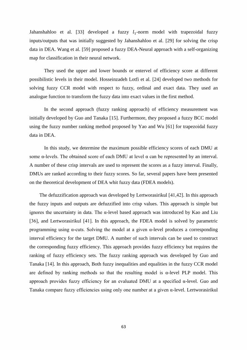
Jahanshahloo et al. [33] developed a fuzzy 𝑙1-norm model with trapezoidal fuzzy
inputs/outputs that was initially suggested by Jahanshahloo et al. [29] for solving the crisp
data in DEA. Wang et al. [59] proposed a fuzzy DEA-Neural approach with a self-organizing
map for classification in their neural network.
They used the upper and lower bounds or entervel of efficiency score at different
possibilistic levels in their model. Hosseinzadeh Lotfi et al. [24] developed two methods for
solving fuzzy CCR model with respect to fuzzy, ordinal and exact data. They used an
analogue function to transform the fuzzy data into exact values in the first method.
In the second approach (fuzzy ranking approach) of efficiency measurement was
initially developed by Guo and Tanaka [15]. Furthermore, they proposed a fuzzy BCC model
using the fuzzy number ranking method proposed by Yao and Wu [61] for trapezoidal fuzzy
data in DEA.
In this study, we determine the maximum possible efficiency scores of each DMU at
some α-levels. The obtained score of each DMU at level α can be represented by an interval.
A number of these crisp intervals are used to represent the scores as a fuzzy interval. Finally,
DMUs are ranked according to their fuzzy scores. So far, several papers have been presented
on the theoretical development of DEA whit fuzzy data (FDEA models).
The defuzzification approach was developed by Lertworasirikul [4 241, ]. In this approach
the fuzzy inputs and outputs are defuzzified into crisp values. This approach is simple but
ignores the uncertainty in data. The α-level based approach was introduced by Kao and Liu
[36], and Lertworasirikul [41]. In this approach, the FDEA model is solved by parametric
programming using α-cuts. Solving the model at a given α-level produces a corresponding
interval efficiency for the target DMU. A number of such intervals can be used to construct
the corresponding fuzzy efficiency. This approach provides fuzzy efficiency but requires the
ranking of fuzzy efficiency sets. The fuzzy ranking approach was developed by Guo and
Tanaka [14]. In this approach, Both fuzzy inequalities and equalities in the fuzzy CCR model
are defined by ranking methods so that the resulting model is α-level PLP model. This
approach provides fuzzy efficiency for an evaluated DMU at a specified α-level. Guo and
Tanaka compare fuzzy efficiencies using only one number at a given α-level. Lertworasirikul
64
et al. [4 241, ] show that for the special case, in which fuzzy membership functions of fuzzy
data are trapezoidal types.
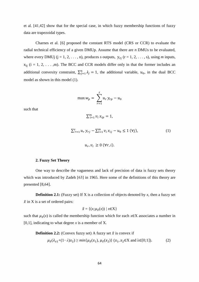
Charnes et al. [6] proposed the constant RTS model (CRS or CCR) to evaluate the
radial technical efficiency of a given DMUp. Assume that there are n DMUs to be evaluated,
where every DMUj (j = 1, 2, . . . , n), produces s outputs, yrj (r = 1, 2, . . . , s), using m inputs,
xij (i = 1, 2, . . . ,m). The BCC and CCR models differ only in that the former includes an
additional convexity constraint, ∑ 𝜆𝑗 = 1𝑛𝑗=1 , the additional variable, 𝑢0, in the dual BCC
model as shown in this model (1).
max𝑤𝑝 = ∑𝑢𝑟
𝑠
𝑟=1
𝑦𝑟𝑝 − 𝑢0
such that
∑ 𝑣𝑖𝑚 𝑖=1 𝑥𝑖𝑝 = 1,
∑ 𝑢𝑟𝑠 𝑟=1 𝑦𝑟𝑗 − ∑ 𝑣𝑖
𝑚𝑖=1 𝑥𝑖𝑗 − 𝑢0 ≤ 1 (∀𝑗), (1)
𝑢𝑟 , 𝑣𝑖 ≥ 0 (∀𝑟, 𝑖).
2. Fuzzy Set Theory
One way to describe the vagueness and lack of precision of data is fuzzy sets theory
which was introduced by Zadeh [63] in 1965. Here some of the definitions of this theory are
presented [8,64].
Definition 2.1: (Fuzzy set) If X is a collection of objects denoted by x, then a fuzzy set
�� in X is a set of ordered pairs:
�� = {(x;𝜇��(x)) | x∈X}
such that 𝜇��(x) is called the membership function which for each x∈X associates a number in
[0,1], indicating to what degree x is a member of X.
Definition 2.2: (Convex fuzzy set) A fuzzy set �� is convex if
𝜇��(𝜆𝑥1+(1−λ)𝑥2) ≥ min{𝜇��(𝑥1), 𝜇��(𝑥2)} (𝑥1, 𝑥2∈X and λ∈[0;1]). (2)

65
Definition 2.3: (Normal fuzzy set) A fuzzy set �� in X is said to be normal if there
exist x∈X such that 𝜇��(x) =1.
Definition 2.4: (Fuzzy number) A fuzzy number �� is a convex normalized fuzzy set ��
of the real line such that
1. There exist exactly one 𝑥0∈ with 𝜇��(𝑥0) = 1 (unimodal).
2. 𝜇��(x) is piecewise continuous.
Definition 2.5: (Positive fuzzy number) A fuzzy number �� is called positive
(negative), denoted by ��>0 (��<0), if its membership function, 𝜇��(x) satisfies, 𝜇��(x) = 0, x <0
(x >0).
Definition 2.6: (LR fuzzy number) A fuzzy number �� is said to be LR if
𝜇��(𝑥) =
{
𝐿 (𝑎−𝑥
𝜎) 𝑥 < 𝑎, 𝜎 > 0
𝑅 (𝑥−𝑏
𝛽) 𝑥 > 𝑏, 𝛽 > 0
, (3)
where σ and β are left and right spreads, respectively, and a function L(.) is the left shape
function satisfying:
1. L(x)=L(−x),
2. L(0)=1 and L(1)=0,
3. L(x) is non-decreasing on [0,∞).
Naturally, a right shape function R(.) is similarly defined as L(.).
Definition 2.7: (LR fuzzy interval) A fuzzy set �� is said to be an LR fuzzy interval if
𝜇��(𝑥) =
{
𝐿 (𝑎−𝑥
𝜎) 𝑥 < 𝑎, 𝜎 > 0
1 𝑎 ≤ 𝑥 ≤ 𝑏
𝑅 (𝑥−𝑏
𝛽) 𝑥 > 𝑏, 𝛽 > 0
, (4)
where [a,b] is the peak or core of 𝑥 and a and b are left and right spreads, respectively, and the
functions L(.) and R(.) are the same as the functions of LR fuzzy number.

66
Definition 2.8: (Triangular fuzzy number) A LR fuzzy number �� is said to be
triangular if L(.) and R(.) be linear functions.
Remark: A membership function of triangular fuzzy number �� = (L;M;R) (L ≤ M ≤ R)
is as follows:
𝜇��(𝑥) = {
(𝑥−𝐿
𝑀−𝐿) 𝐿 ≤ 𝑥 < 𝑀
1 𝑥 = 𝑀
(𝑥−𝑅
𝑀−𝑅) 𝑀 < 𝑥 ≤ 𝑅
. (5)
Definition 2.9: (Trapezoidal fuzzy number) �� = (𝑥0 , 𝑦0 , 𝜎 , 𝛽) with two defuzzifier
𝑥0 , 𝑦0 and left fuzziness σ>0 and right fuzziness β>0 is a fuzzy set where the membership
function is as:
𝜇��(𝑥) =
{
1
𝜎(𝑥 − 𝑥0 + 𝜎) 𝑥0 − 𝜎 ≤ 𝑥 ≤ 𝑥0
1 𝑥 ∈ [𝑥0, 𝑦0]1
𝛽(𝑦0 − 𝑥 + 𝛽) 𝑦0 ≤ 𝑥 ≤ 𝑦0 + 𝛽
0 𝑜𝑡ℎ𝑒𝑟𝑤𝑖𝑠𝑒
. (6)
4. Introduction to Theory
In this section, we review some basic definitions of fuzzy sets [11,35,65].
Definition 3.1: A fuzzy number �� in parametric form is a pair (��𝑖 , ��𝑑 ) of functions
��𝑖 (𝑟), ��𝑑 (𝑟), 0 ≤ 𝑟 ≤ 1, which satisfy the following requirements:
1. ��𝑖 is a bounded monotonic increasing left continuous function,
2. ��𝑑 is a bounded monotonic decreasing left continuous function,
3. ��𝑖 ≤ ��𝑑 , 0 ≤ 𝑟 ≤ 1
and its parametric form is
��𝑖 (𝑟) = (𝑥0 − 𝜎 + 𝜎𝑟), ��𝑑 (𝑟) = (𝑦0 + 𝛽 − 𝛽𝑟).
Provided that, 𝑥0 =𝑦0 then �� is a triangular fuzzy number, and we write �� = (𝑥0 , 𝜎 , 𝛽).
Definition 3.2: The support of fuzzy number �� is defined as follows:
Supp(��)={𝑥 𝜇��(𝑥) > 0} ,
where {𝑥 𝜇��(𝑥) > 0} is closure of set {𝑥 𝜇��(𝑥) > 0}.

67
Definition 3.3: The addition and scalar multiplication of fuzzy numbers are defined by
the extension principle and can be equivalently represented in [8,62,65] as follows. For
arbitrary �� = (��𝑖 , ��𝑑 ), �� =(��𝑖 , ��𝑑 ) we define addition �� + �� and multiplication by scalar k >
0 as:
(��𝑖 + ��𝑖 )(𝑟) = ��𝑖 (𝑟) + ��𝑖 (𝑟) , (��𝑑 + ��𝑑 )(𝑟) = ��𝑑 (𝑟) + ��𝑑 (𝑟) ,
(𝑘�� )𝑖(𝑟) = 𝑘��𝑖 (𝑟) , (𝑘�� )
𝑑(𝑟) = 𝑘��𝑑 (𝑟) , (7)
(𝑘�� )𝑖(𝑟) = 𝑘��𝑖 (𝑟), (𝑘�� )
𝑑(𝑟) = 𝑘��𝑑 (𝑟).
To emphasis the collection of all fuzzy numbers with addition and multiplication as
defined by (7) is denoted by E, which is a convex cone. The image (opposite) of �� =
(𝑥0 , 𝑦0 , 𝜎 , 𝛽) can be defined by − �� =(−𝑥0 , −𝑦0 , 𝛽, 𝜎), see [26,65].
Definition 3.4: (α-cut of fuzzy set) A α-cut of fuzzy set �� is α crisp subset of X which,
denoted by:
��𝛼 = {x∈X|𝜇��(x) ≥ α} = [𝑥𝛼𝐿;𝑥𝛼𝑈] = [𝑋𝑚𝑖𝑛{x∈X|𝜇��(x) ≥α}
;𝑋𝑚𝑎𝑥{x∈X|𝜇��(x) ≥α}] (8)
The α-cuts of �� and �� are defined as:
��𝛼 = {x∈X|𝜇��(x) ≥ α} = [𝑥𝛼𝐿;𝑥𝛼𝑈], (9)
and
��𝛼={x∈X|𝜇��(x) ≥ α} = [𝑦𝛼𝐿;𝑦𝛼𝑈] (10)
We can draw a membership function of triangular fuzzy number with concept of local
α-cut .
Definition 3.5: The trapezoidal fuzzy number �� = (𝑥0 , 𝑦0 , 𝜎 , 𝛽) is reduced to a real
number �� 𝑖𝑓 𝑥0 = 𝑦0 = 𝜎 = 𝛽 . Conversely, a real number u can be written as a trapezoidal
fuzzy number �� = (𝑥, 𝑥, 𝑥, 𝑥). Similarly, the α-level �� = (𝑥0 , 𝑦0 , 𝜎 , 𝛽) can easily be
determined as:
[��]𝛼 = [𝛼𝑥0 + (1 − 𝛼)𝜎, 𝛼𝑦0 + (1 − 𝛼)𝛽] , (11)

68
where 𝛼 ∈ [0,1]. If x = 𝑥0 = 𝑦0, then �� = (𝑥0 , 𝜎 , 𝛽) is called a triangular fuzzy number.
Definition 3.6: x real fuzzy number �� denoted by �� = (𝑥0 , 𝑦0 , 𝜎 , 𝛽, 𝑤) is described as
any fuzzy subset of the real line with a membership function 𝜇��, which satisfies the
following properties:
𝜇�� is a semicontinuous mapping from to the closed interval [0,w] (0 ≤ w ≤1),
𝜇��(x) = 0 for all x ∈ [-∞,σ],
𝜇�� is increasing on [σ,𝑥0],
𝜇��(x) = w for all x ∈ [𝑥0,𝑦0], where w is a constant and 0 < w ≤ 1,
𝜇�� is decreasing on [𝑦0,β],
𝜇��(x) = 0 for all x ∈ [β,∞],
where 𝑥0, 𝑦0, 𝜎 and 𝛽 are real numbers.
Unless elsewhere specified, it is assumed that �� is convex and bounded, i.e., −∞ < σ,
β < ∞. If w = 1, �� is a normal fuzzy number, and if 0 < w < 1, �� is a nonnormal fuzzy number.
Definition 3.7: Suppose that we have two positive trapezoidal fuzzy numbers �� =
(𝑥𝑎, 𝑦𝑎, 𝜎𝑎, 𝛽𝑎) and �� = (𝑥𝑏 , 𝑦𝑏 , 𝜎𝑏 , 𝛽𝑏), then the arithmetic operations of these two
trapezoidal fuzzy numbers are defined as follows:
��(+)�� = (𝑥𝑎 + 𝑥𝑏 , 𝑦𝑎+𝑦𝑏 , 𝜎𝑎 + 𝜎𝑏 , 𝛽𝑎 + 𝛽𝑏 ),
��(−)�� = (𝑥𝑎 − 𝑥𝑏 , 𝑦𝑎−𝑦𝑏 , 𝜎𝑎 − 𝜎𝑏 , 𝛽𝑎 − 𝛽𝑏 ),
��(×)�� = (𝑥𝑎𝑥𝑏 , 𝑦𝑎𝑦𝑏 , 𝜎𝑎𝜎𝑏𝐴 , 𝛽𝑎𝛽𝑏 ),
𝑘�� = (𝑘𝑥𝑎 , 𝑘𝑦𝑎, 𝑘𝜎𝑎, 𝑘𝛽𝑎) (∀ 𝑘 ∈ +),
𝑘�� = (𝑘𝑥𝑏 , 𝑘𝑦𝑏 , 𝑘𝜎𝑏 , 𝑘𝛽𝑏) (∀ 𝑘 ∈ +),
(��)−1 = (1
𝑦𝑎,1
𝑥𝑎,1
𝛽𝑎,1
𝜎𝑎), (��)−1 = (
1
𝑦𝑏,1
𝑥𝑏,1
𝛽𝑏,1
𝜎𝑏),
��(÷)�� = ��(×)��−1 = (𝑥𝑎
𝑦𝑏,𝑦𝑎
𝑥𝑏,𝜎𝑎
𝛽𝑏,𝛽𝑎
𝜎𝑏).
Definition 3.8: An alternative way of fuzzy arithmetic can be defined based on the
interval of the arithmetic of α-level intervals. The interval arithmetic If �� and �� be two fuzzy
numbers with α-level intervals ��𝛼 = [��𝛼𝐿 , ��𝛼𝑈] and ��𝛼 = [��𝛼𝐿 , ��𝛼𝑈] then the Definition 3.7
can be achieved as follows:
��𝛼(+)��𝛼=[��𝛼𝐿 + ��𝛼𝐿 , ��𝛼𝑈 + ��𝛼𝑈],
��𝛼(−)��𝛼=[��𝛼𝐿 − ��𝛼𝐿 , ��𝛼𝑈 − ��𝛼𝑈],
69
��𝛼(×)��𝛼=[𝑚𝑖𝑛{��𝛼𝐿��𝛼𝐿 , ��𝛼𝐿��𝛼𝑈, ��𝛼𝑈��𝛼𝐿 , ��𝛼𝑈��𝛼𝑈},
𝑚𝑎𝑥{��𝛼𝐿��𝛼𝐿 , ��𝛼𝐿��𝛼𝑈, ��𝛼𝑈��𝛼𝐿 , ��𝛼𝑈��𝛼𝑈}],
(��𝛼)−1=[1
��𝛼𝐿,1
��𝛼𝑈], (��𝛼)−1=[
1
��𝛼𝐿,1
��𝛼𝑈],
��𝛼(÷)��𝛼 = ��(×)��−1 = ��𝛼(×)1
��𝛼 .
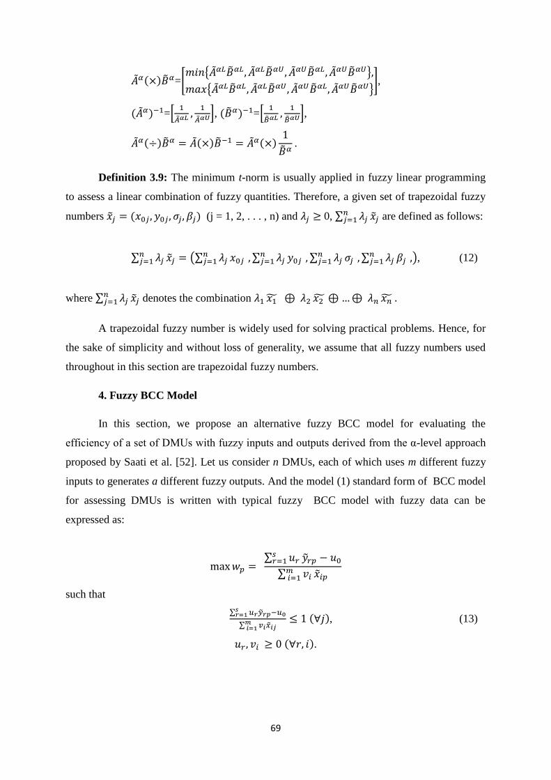
Definition 3.9: The minimum t-norm is usually applied in fuzzy linear programming
to assess a linear combination of fuzzy quantities. Therefore, a given set of trapezoidal fuzzy
numbers ��𝑗 = (𝑥0𝑗 , 𝑦0𝑗, 𝜎𝑗, 𝛽𝑗) (j = 1, 2, . . . , n) and 𝜆𝑗 ≥ 0, ∑ 𝜆𝑗 ��𝑗𝑛𝑗=1 are defined as follows:
∑ 𝜆𝑗 ��𝑗𝑛𝑗=1 = (∑ 𝜆𝑗 𝑥0𝑗 ,
𝑛𝑗=1 ∑ 𝜆𝑗 𝑦0𝑗 ,
𝑛𝑗=1 ∑ 𝜆𝑗 𝜎𝑗 ,
𝑛𝑗=1 ∑ 𝜆𝑗 𝛽𝑗 ,
𝑛𝑗=1 ), (12)
where ∑ 𝜆𝑗 ��𝑗𝑛𝑗=1 denotes the combination 𝜆1 𝑥1 ⊕ 𝜆2 𝑥2 ⊕ …⊕ 𝜆𝑛 𝑥�� .
A trapezoidal fuzzy number is widely used for solving practical problems. Hence, for
the sake of simplicity and without loss of generality, we assume that all fuzzy numbers used
throughout in this section are trapezoidal fuzzy numbers.
4. Fuzzy BCC Model
In this section, we propose an alternative fuzzy BCC model for evaluating the
efficiency of a set of DMUs with fuzzy inputs and outputs derived from the α-level approach
proposed by Saati et al. [52]. Let us consider n DMUs, each of which uses m different fuzzy
inputs to generates a different fuzzy outputs. And the model (1) standard form of BCC model
for assessing DMUs is written with typical fuzzy BCC model with fuzzy data can be
expressed as:
max𝑤𝑝 = ∑ 𝑢𝑟𝑠𝑟=1 ��𝑟𝑝 − 𝑢0∑ 𝑣𝑖𝑚 𝑖=1 ��𝑖𝑝
such that
∑ 𝑢𝑟𝑠𝑟=1 ��𝑟𝑝−𝑢0
∑ 𝑣𝑖𝑚 𝑖=1 ��𝑖𝑗
≤ 1 (∀𝑗), (13)
𝑢𝑟 , 𝑣𝑖 ≥ 0 (∀𝑟, 𝑖).
70
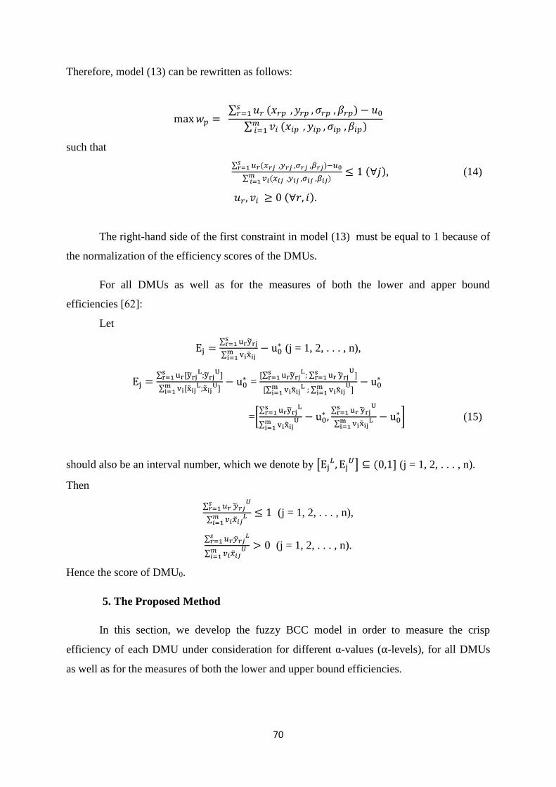
Therefore, model (13) can be rewritten as follows:
max𝑤𝑝 = ∑ 𝑢𝑟𝑠𝑟=1 (𝑥𝑟𝑝 , 𝑦𝑟𝑝 , 𝜎𝑟𝑝 , 𝛽𝑟𝑝) − 𝑢0∑ 𝑣𝑖𝑚 𝑖=1 (𝑥𝑖𝑝 , 𝑦𝑖𝑝 , 𝜎𝑖𝑝 , 𝛽𝑖𝑝)
such that
∑ 𝑢𝑟𝑠𝑟=1 (𝑥𝑟𝑗 ,𝑦𝑟𝑗 ,𝜎𝑟𝑗 ,𝛽𝑟𝑗)−𝑢0
∑ 𝑣𝑖𝑚 𝑖=1 (𝑥𝑖𝑗 ,𝑦𝑖𝑗 ,𝜎𝑖𝑗 ,𝛽𝑖𝑗)
≤ 1 (∀𝑗), (14)
𝑢𝑟 , 𝑣𝑖 ≥ 0 (∀𝑟, 𝑖).
The right-hand side of the first constraint in model (13) must be equal to 1 because of
the normalization of the efficiency scores of the DMUs.
For all DMUs as well as for the measures of both the lower and apper bound
efficiencies [62]:
Let
Ej =∑ uryrjsr=1
∑ vimi=1 xij
− u0∗ (j = 1, 2, . . . , n),
Ej =∑ ur[sr=1 yrj
L;yrjU]
∑ vimi=1 [xij
L;xijU]− u0
∗ = [∑ ur
sr=1 yrj
L; ∑ ursr=1 yrj
U]
[∑ vimi=1 xij
L ; ∑ vimi=1 xij
U]− u0
∗
=[∑ ursr=1 yrj
L
∑ vimi=1 xij
U − u0∗ ,∑ ursr=1 yrj
U
∑ vimi=1 xij
L − u0∗] (15)
should also be an interval number, which we denote by [Ej𝐿 , Ej
𝑈] ⊆ (0,1] (j = 1, 2, . . . , n).
Then
∑ 𝑢𝑟𝑠𝑟=1 ��𝑟𝑗
𝑈
∑ 𝑣𝑖𝑚𝑖=1 ��𝑖𝑗
𝐿 ≤ 1 (j = 1, 2, . . . , n),
∑ 𝑢𝑟𝑠𝑟=1 ��𝑟𝑗
𝐿
∑ 𝑣𝑖𝑚𝑖=1 ��𝑖𝑗
𝑈 > 0 (j = 1, 2, . . . , n).
Hence the score of DMU0.
5. The Proposed Method
In this section, we develop the fuzzy BCC model in order to measure the crisp
efficiency of each DMU under consideration for different α-values (α-levels), for all DMUs
as well as for the measures of both the lower and upper bound efficiencies.
71
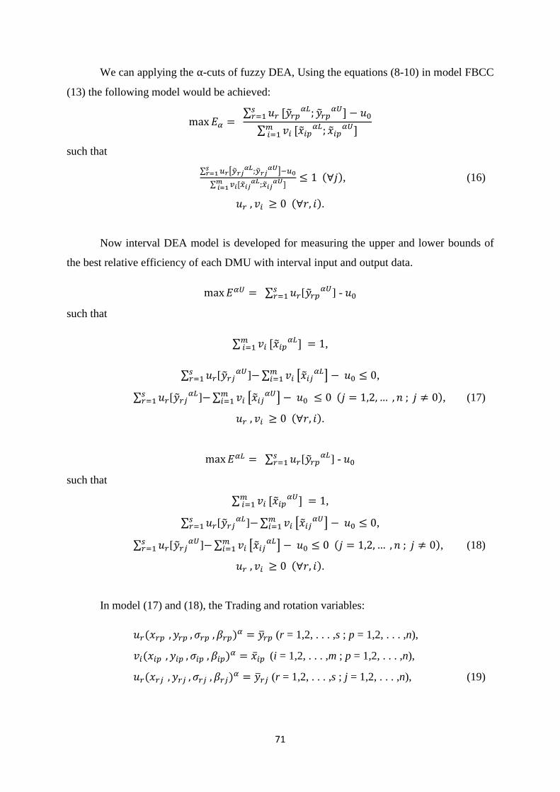
We can applying the α-cuts of fuzzy DEA, Using the equations (8-10) in model FBCC
(13) the following model would be achieved:
max𝐸𝛼 = ∑ 𝑢𝑟𝑠𝑟=1 [��𝑟𝑝
𝛼𝐿; ��𝑟𝑝𝛼𝑈] − 𝑢0
∑ 𝑣𝑖𝑚 𝑖=1 [��𝑖𝑝
𝛼𝐿; ��𝑖𝑝𝛼𝑈]
such that
∑ 𝑢𝑟[��𝑟𝑗𝛼𝐿;��𝑟𝑗
𝛼𝑈]𝑠𝑟=1 −𝑢0
∑ 𝑣𝑖𝑚 𝑖=1 [��𝑖𝑗
𝛼𝐿;��𝑖𝑗𝛼𝑈]
≤ 1 (∀𝑗), (16)
𝑢𝑟 , 𝑣𝑖 ≥ 0 (∀𝑟, 𝑖).
Now interval DEA model is developed for measuring the upper and lower bounds of
the best relative efficiency of each DMU with interval input and output data.
max𝐸𝛼𝑈 = ∑ 𝑢𝑟𝑠𝑟=1 [��𝑟𝑝
𝛼𝑈] - 𝑢0
such that
∑ 𝑣𝑖𝑚 𝑖=1 [��𝑖𝑝
𝛼𝐿] = 1,
∑ 𝑢𝑟𝑠𝑟=1 [��𝑟𝑗
𝛼𝑈]−∑ 𝑣𝑖𝑚𝑖=1 [��𝑖𝑗
𝛼𝐿] − 𝑢0 ≤ 0,
∑ 𝑢𝑟𝑠𝑟=1 [��𝑟𝑗
𝛼𝐿]−∑ 𝑣𝑖𝑚𝑖=1 [��𝑖𝑗
𝛼𝑈] − 𝑢0 ≤ 0 (𝑗 = 1,2, … , 𝑛 ; 𝑗 ≠ 0), (17)
𝑢𝑟 , 𝑣𝑖 ≥ 0 (∀𝑟, 𝑖).
max𝐸𝛼𝐿 = ∑ 𝑢𝑟𝑠𝑟=1 [��𝑟𝑝
𝛼𝐿] - 𝑢0
such that
∑ 𝑣𝑖𝑚 𝑖=1 [��𝑖𝑝
𝛼𝑈] = 1,
∑ 𝑢𝑟𝑠𝑟=1 [��𝑟𝑗
𝛼𝐿]−∑ 𝑣𝑖𝑚𝑖=1 [��𝑖𝑗
𝛼𝑈] − 𝑢0 ≤ 0,
∑ 𝑢𝑟𝑠𝑟=1 [��𝑟𝑗
𝛼𝑈]−∑ 𝑣𝑖𝑚𝑖=1 [��𝑖𝑗
𝛼𝐿] − 𝑢0 ≤ 0 (𝑗 = 1,2, … , 𝑛 ; 𝑗 ≠ 0), (18)
𝑢𝑟 , 𝑣𝑖 ≥ 0 (∀𝑟, 𝑖).
In model (17) and (18), the Trading and rotation variables:
𝑢𝑟(𝑥𝑟𝑝 , 𝑦𝑟𝑝 , 𝜎𝑟𝑝 , 𝛽𝑟𝑝)𝛼 = ��𝑟𝑝 (r = 1,2, . . . ,s ; p = 1,2, . . . ,n),
𝑣𝑖(𝑥𝑖𝑝 , 𝑦𝑖𝑝 , 𝜎𝑖𝑝 , 𝛽𝑖𝑝)𝛼 = ��𝑖𝑝 (i = 1,2, . . . ,m ; p = 1,2, . . . ,n),
𝑢𝑟(𝑥𝑟𝑗 , 𝑦𝑟𝑗 , 𝜎𝑟𝑗 , 𝛽𝑟𝑗)𝛼 = ��𝑟𝑗 (r = 1,2, . . . ,s ; j = 1,2, . . . ,n), (19)

72
𝑣i(xij , yij , σij , βij)α = xij (i = 1,2, . . . ,m ; j = 1,2, . . . ,n)
are introduced to receive the following program:
maxEαU = ∑ yrpUs
r=1 - u0
such that
∑ xip Lm
i=1 = 1,
∑ yrjUs
r=1 − ∑ xijL − u0
mi=1 ≤ 0,
∑ yrjLs
r=1 − ∑ xijU − u0
mi=1 ≤ 0 (𝑗 = 1,2, … , 𝑛 ; 𝑗 ≠ 0) (20)
ur , 𝑣i ≥ 0 (∀r, i) , u0 uncertain.
maxEαL = ∑ yrpLs
r=1 - u0
such that
∑ xip Um
i=1 = 1,
∑ yrjLs
r=1 − ∑ xijUm
i=1 − u0 ≤ 0,
∑ yrjUs
r=1 − ∑ xijLm
i=1 − u0 ≤ 0 (𝑗 = 1,2, … , 𝑛 ; 𝑗 ≠ 0) (21)
ur , 𝑣i ≥ 0 (∀r, i) , u0 uncertain.
The fuzzy linear programming problem given by (20) and (21) is equivalent to a crisp
parametric linear programming problem. Using the optimal value, we can determine the
situation for returns to scale RTS when a DMUp is efficient. Similar to the conventional DEA
model of Banker and Thrall [3].
From (15) the lower and upper bounds of the efficiency score for a given α can be
reduced as:
𝐸𝑗=[∑ 𝑢𝑟
∗𝑠𝑟=1 [𝛼𝑥𝑟𝑝 +(1−𝛼)𝜎𝑟𝑝 ]
∑ 𝑣𝑖∗𝑚
𝑖=1 [𝛼𝑦𝑖𝑝 +(1−𝛼)𝛽𝑖𝑝 ]− 𝑢0
∗ ,∑ 𝑢𝑟
∗𝑠𝑟=1 [𝛼𝑦𝑟𝑝 +(1−𝛼)𝛽𝑟𝑝]
∑ 𝑣𝑖∗𝑚
𝑖=1 [𝛼𝑥𝑖𝑝 +(1−𝛼)𝜎𝑖𝑝 ]− 𝑢0
∗].
We can applying the α-level of fuzzy DEA. Using the equations (11) in model FBCC
(13) the following model would be achieved:

73
max𝑤𝑝 = ∑ 𝑢𝑟𝑠𝑟=1 [αxrp + (1 − α)σrp , αyrp + (1 − α)βrp] − 𝑢0
∑ 𝑣𝑖𝑚 𝑖=1 [αxip + (1 − α)σip , αyip + (1 − α)βip]
such that
∑ 𝑢𝑟𝑠𝑟=1 [𝛼𝑥𝑟𝑗 +(1−𝛼)𝜎𝑟𝑗 ,𝛼𝑦𝑟𝑗 +(1−𝛼)𝛽𝑟𝑗]−𝑢0
∑ 𝑣𝑖𝑚 𝑖=1 [𝛼𝑥𝑖𝑗 + (1−𝛼)𝜎𝑖𝑗 ,𝛼𝑦𝑖𝑗 +(1−𝛼)𝛽𝑖𝑗]
≤ 1 (∀𝑗), (22)
ur , 𝑣i ≥ 0 (∀r, i) , u0 uncertain,
where ��𝑟𝑗 = (𝑥𝑟𝑗 , 𝑦𝑟𝑗 , 𝜎𝑟𝑗 , 𝛽𝑟𝑗) and ��𝑖𝑗 = (𝑥𝑖𝑗 , 𝑦𝑖𝑗 , 𝜎𝑖𝑗 , 𝛽𝑖𝑗) are the rth fuzzy output and ith
fuzzy input values of the jth DMU, respectively, are characterized as trapezoidal fuzzy
numbers.
Model (22) is an interval programming model that can be solved by standard
optimization methods. Hence, we transform the interval model (22) into a programming
model using the following interval alteration variables:
[αxrp + (1 − α)σrp , αyrp + (1 − α)βrp]=yrp (∀r , p)
[αxip + (1 − α)σip , αyip + (1 − α)βip ]=xip (∀i , p)
[αxrj + (1 − α)σrj , αyrj + (1 − α)βrj] = yrj (∀r , j) (23)
[αxij + (1 − α)σij , αyij + (1 − α)βij] = xij (∀i , j) .
The substitutions of the above interval alteration variables in model (22) will result in
the following programming model:
max𝑤𝑝 = ∑ 𝑢𝑟𝑠𝑟=1 yrp − 𝑢0∑ 𝑣𝑖𝑚 𝑖=1 xip
such that
∑ 𝑢𝑟yrj𝑠𝑟=1 −𝑢0
∑ 𝑣𝑖𝑚 𝑖=1 xij
≤ 1 (∀𝑗), (24)
𝑢𝑟 , 𝑣𝑖 ≥ 0 (∀𝑟 , 𝑖).
In model (24), the alternation variables as:
𝑢𝑟yrp = ��𝑟𝑝(r = 1, 2, . . . , s, p = 1, 2, . . . , n),
𝑣𝑖xip = ��𝑖𝑝 (i = 1, 2, . . . , m, p = 1, 2, . . . , n),
𝑢ryrj = ��𝑟𝑗(r = 1, 2, . . . , s, j = 1, 2, . . . , n), (25)

74
𝑣𝑖xij = ��𝑖𝑗 (𝑖 = 1, 2, . . . , 𝑚 ; j = 1, 2, . . . , 𝑛)
are introduced to receive the following program:
max∑��𝑟𝑝
s
r=1
− 𝑢0
such that
∑ ��𝑖𝑝m i=1 = 1,
∑ ��𝑟𝑗sr=1 − ∑ ��𝑖𝑗
mi=1 − 𝑢0 ≤ 0 (𝑗 ≠ 𝑝), (26)
𝑢𝑟(αxrj + (1 − α)σrj) ≤ ��𝑟𝑗 ≤ 𝑢𝑟(αyrj + (1 − α)βrj) (∀r , j),
𝑣𝑖(αxij + (1 − α)σij) ≤ ��𝑖𝑗 ≤ 𝑣𝑖(αyij + (1 − α)βij) (∀i , j),
ur , vi ≥ 0 (∀r , i) , u0 uncertain.
Model (26) is equivalent to a intervel programming model with α ∈ [0,1]. Therefore,
analyzing the efficiency of DMUs with the proposed method, for a set of n different values of
α, e.g. αi (i = 1,2, ... ,n). Therefore, it will be necessary to obtain an integrated efficiency score
for DMUs to rank them. The fuzzy linear programming problem given by (26) is equivalent to
a crisp intervel linear programming problem. Using the optimal value, we can determine the
situation for returns to scale RTS for BCC and CCR when a DMUp is efficient. Similar to the
conventional DEA model of Banker and Thrall [3].
From (15) the intervel of the efficiency score for a given α can be reduced as:
Ej=[
∑ ur∗s
r=1 [αxrj +(1−α)σrj]
∑ vi∗m
i=1 [αyij + (1−α)βij]− u0
∗ ,∑ ur
∗sr=1 [αxrj +(1−α)σrj]
∑ vi∗m
i=1 [αxij +(1−α)σij]− u0
∗
,∑ ur
∗sr=1 [αyrj +(1−α)βrj]
∑ vi∗m
i=1 [αyij + (1−α)βij]− u0
∗ ,∑ ur
∗sr=1 [αyrj +(1−α)βrj]
∑ vi∗m
i=1 [αxij +(1−α)σij]− u0
∗].
6. Numerical Examples
In this section, we use two numerical examples, Saati et. al. [53] and Guo and Tanaka
[15] are solved by the proposed method and the results are compared with previously
presented methods.
Example 1. Consider 4 DMUs with inputs and outputs which are presented in Table 1,
this problem results are compared with two previously presented Kao and Liu [36] and
Razavi, et. al. [51].

75
Table 1: Inputs and outputs of 4 DMUs.
DMU Input α-cut Output α-cut
A (11,12,14) [11+ α,14-2 α] 10 [10,10]
B 30 [30,30] (12,13,14,16) [12+ α,16-2 α]
C 40 [40,40] 11 [11,11]
D (45,47,52,55) [45+2 α,55-3 α] (12,15,19,22) [12+3 α,22-3 α]
Considering the DMU D, by FBCC models (20,21) for upper and lower objective
models are solved:
max𝐸𝛼𝑈(𝐷) = 𝑚𝑎𝑥 (22 − 3α) 𝑢1 − 𝑢0
such that
(45 + 2α)𝑣1 = 1
10𝑢1 − (11 + α)𝑣1 − 𝑢0 ≤ 0
(16 − 2α)𝑢1 − 30𝑣1 − 𝑢0 ≤ 0
11𝑢1 − 40 𝑣1 − 𝑢0 ≤ 0
(22 − 3α)𝑢1 − (45 + 2α)𝑣1 − 𝑢0 ≤ 0
10𝑢1 − (14 − 2𝛼)𝑣1 − 𝑢0 ≤ 0
(12 + α)𝑢1 − 30𝑣1 − 𝑢0 ≤ 0
11𝑢1 − 40 𝑣1 − 𝑢0 ≤ 0
(22 − 3α)𝑢1 − (55 + 3α)𝑣1 − 𝑢0 ≤ 0
𝑢1 , 𝑣1 ≥ 0 , 𝑢0 ∶ 𝑢𝑛𝑟𝑒𝑠𝑡𝑟𝑖𝑐𝑡𝑒𝑑 .
max𝐸𝛼𝐿(𝐷) = 𝑚𝑎𝑥 (12 + 3α) 𝑢1 − 𝑢0
such that
(55 + 3α)𝑣1 = 1
10𝑢1 − (14 − 2𝛼)𝑣1 − 𝑢0 ≤ 0
(12 + α)𝑢1 − 30𝑣1 − 𝑢0 ≤ 0
11𝑢1 − 40 𝑣1 − 𝑢0 ≤ 0
(22 − 3α)𝑢1 − (55 + 3α)𝑣1 − 𝑢0 ≤ 0
10𝑢1 − (11 + α)𝑣1 − 𝑢0 ≤ 0
(16 − 2α)𝑢1 − 30𝑣1 − 𝑢0 ≤ 0

76
11𝑢1 − 40 𝑣1 − 𝑢0 ≤ 0
(22 − 3α)𝑢1 − (45 + 2α)𝑣1 − 𝑢0 ≤ 0
𝑢1 , 𝑣1 ≥ 0 , 𝑢0 ∶ 𝑢𝑛𝑟𝑒𝑠𝑡𝑟𝑖𝑐𝑡𝑒𝑑 .
The results for these models are solved for different α-values in Table 2.
Table 2: The α-cuts of the efficiency at four α-values on the proposed method and two previously presented.
A[EαL, EαU] B[EαL, EαU]
Α Proposed
BCC Kao and Liu Razavi et.al.
Proposed
BCC Kao and Liu
Razavi and
et.al.
0.0 [0.98,1.0] [1.0,1.0] 0.9497 [0.72,1.0] [0.71,1.0] [0.71,0.95]
0.5 [0.98,1.0] [1.0,1.0] 0.9725 [0.80,1.0] [0.79,1.0] [0.79,0.95]
0.75 [0.98,1.0] [1.0,1.0] 0.9873 [0.82,1.0] [0.83,1.0] [0.83,0.95]
1.0 [0.98,1.0] [1.0,1.0] 1.0 [0.90,1.0] [0.88,1.0] [0.88,0.95]
C[EαL, EαU] D[EαL, EαU]
Α Proposed
BCC Kao and Liu
Razavi and
et.al.
Proposed
BCC Kao and Liu
Razavi and
et.al.
0.0 [0.58,1.0] [0.54,0.91] 0.5436 [0.72,1.0] [0.74,1.0] [0.54,1.0]
0.5 [0.61,1.0] [0.58,0.85] 0.5890 [0.79,1.0] [0.89,1.0] [0.65,1.0]
0.75 [0.64,1.0] [0.60,0.82] 0.6086 [0.91,1.0] [0.96,1.0] [0.70,1.0]
1.0 [0.70,1.0] [0.63,0.79] 0.6395 [0.96,1.0] [1.0,1.0] [0.78,1.0]
Table 3: The results for model (20,21) and the ranking of each DMU for different α-levels.
Interval Score
α = 0 Rank α = 0.5 Rank α = 0.75 Rank α = 1.0 Rank
A [0.98,1.0] 1 [0.98,1.0] 1 [0.98,1.0] 1 [0.98,1.0] 1
B [0.72,1.0] 2 [0.80,1.0] 2 [0.82,1.0] 3 [0.90,1.0] 3
C [0.58,1.0] 4 [0.61,1.0] 4 [0.64,1.0] 4 [0.70,1.0] 4
D [0.72,1.0] 3 [0.79,1.0] 3 [0.91,1.0] 2 [0.96,1.0] 2

77
Example 2. Consider 5 DMUs with 2 inputs and 2 outputs which are presented in
Table 4, this problem results are compared with six previously presented Guo and Tanaka
[15], Lertworasirikul et al. [41,42], Saati et al. [52] and Majid et. al. [45].
Table 4: 2 Inputs and 2 outputs of 5 DMUs.
DMU Input 1 Input 2 Output 1 Output 2
A (3.5,4,4.5) (1.9,2.1,2.3) (2.4,2.6,2.8) (3.8,4.1,4.4)
B (2.9,2.9,2.9) (1.4,1.5,1.6) (2.2,2.2,2.2) (3.3,3.5,3.7)
C (4.4,4.9,5.4) (2.2,2.6,3.2) (2.7,3.2,3.7) (4.3,5.1,5.9)
D (3.4,4.1,4.8) (2.2,2.3,2.4) (2.5,2.9,3.3) (5.5,5.7,5.9)
E (5.9,6.5,7.1) (3.6,4.1,4.6) (4.4,5.1,5.8) (6.5,7.4,8.3)
Considering the DMU D, by FBCC model (26) for intervel of the objective models are
solved:
max𝐸𝛼(𝐴) = 𝑚𝑎𝑥 (��11 + ��21) − 𝑢0
such that
��11 + ��21 = 1
(��11 + ��21) − (��11 + ��21 ) − 𝑢0 ≤ 0
(��12 + ��22) − (��12 + ��22 ) − 𝑢0 ≤ 0
(��13 + ��23) − (��13 + ��23 ) − 𝑢0 ≤ 0
(��14 + ��24) − (��14 + ��24 ) − 𝑢0 ≤ 0
(��15 + ��25) − (��15 + ��25 ) − 𝑢0 ≤ 0
𝑢1(α(2.4) + (1 − α)2.6) ≤ ��11 ≤ 𝑢1(α(2.4) + (1 − α)2.8)
𝑢1(α(2.2) + (1 − α)2.2) ≤ ��12 ≤ 𝑢1(α(2.2) + (1 − α)2.2)
𝑢1(α(2.7) + (1 − α)3.2) ≤ ��13 ≤ 𝑢1(α(2.7) + (1 − α)3.7)
𝑢1(α(2.5) + (1 − α)2.9) ≤ ��14 ≤ 𝑢1(α(2.5) + (1 − α)3.3)
𝑢1(α(4.4) + (1 − α)5.1) ≤ ��15 ≤ 𝑢1(α(4.4) + (1 − α)5.8)

78
𝑢2(α(3.8) + (1 − α)4.1) ≤ ��11 ≤ 𝑢2(α(3.8) + (1 − α)4.4)
𝑢2(α(3.3) + (1 − α)3.5. ) ≤ ��12 ≤ 𝑢2(α(3.3) + (1 − α)3.7)
𝑢2(α(4.3) + (1 − α)5.1) ≤ ��13 ≤ 𝑢2(α(4.3) + (1 − α)5.9)
𝑢2(α(5.5) + (1 − α)5.7) ≤ ��14 ≤ 𝑢2(α(5.5) + (1 − α)5.9)
𝑢2(α(6.5) + (1 − α)7.4) ≤ ��15 ≤ 𝑢2(α(6.5) + (1 − α)8.3)
𝑣1(α(3.5) + (1 − α)4.0 ≤ ��11 ≤ 𝑣1(α(3.5) + (1 − α)4.5)
𝑣1(α(2.9) + (1 − α)2.9 ≤ ��12 ≤ 𝑣1(α(2.9) + (1 − α)2.9)
𝑣1(α(4.4) + (1 − α)4.9 ≤ ��13 ≤ 𝑣1(α(4.4) + (1 − α)5.4)
𝑣1(α(3.4) + (1 − α)4.1 ≤ ��14 ≤ 𝑣1(α(3.4) + (1 − α)4.8)
𝑣1(α(5.9) + (1 − α)6.5 ≤ ��15 ≤ 𝑣1(α(5.9) + (1 − α)7.1)
𝑣2(α(1.9) + (1 − α)2.1 ≤ ��11 ≤ 𝑣2(α(1.9) + (1 − α)2.3)
𝑣2(α(1.4) + (1 − α)1.5 ≤ ��12 ≤ 𝑣2(α(1.4) + (1 − α)1.6)
𝑣2(α(2.2) + (1 − α)2.6 ≤ ��13 ≤ 𝑣2(α(2.2) + (1 − α)3.0)
𝑣2(α(2.2) + (1 − α)2.3 ≤ ��14 ≤ 𝑣2(α(2.2) + (1 − α)2.4)
𝑣2(α(3.6) + (1 − α)4.1 ≤ ��15 ≤ 𝑣2(α(3.6) + (1 − α)4.6)
𝑢1 , 𝑣1 , 𝑢2 , 𝑣2 ≥ 0 , 𝑢0 ∶ 𝑢𝑛𝑟𝑒𝑠𝑡𝑟𝑖𝑐𝑡𝑒𝑑 .
max𝐸𝛼(𝐵) = 𝑚𝑎𝑥 (��12 + ��22) − 𝑢0
such that
��12 + ��22 = 1
(��11 + ��21) − (��11 + ��21 ) − 𝑢0 ≤ 0
(��12 + ��22) − (��12 + ��22 ) − 𝑢0 ≤ 0
(��13 + ��23) − (��13 + ��23 ) − 𝑢0 ≤ 0
(��14 + ��24) − (��14 + ��24 ) − 𝑢0 ≤ 0
(��15 + ��25) − (��15 + ��25 ) − 𝑢0 ≤ 0

79
𝑢1(α(2.4) + (1 − α)2.6) ≤ ��11 ≤ 𝑢1(α(2.4) + (1 − α)2.8)
𝑢1(α(2.2) + (1 − α)2.2) ≤ ��12 ≤ 𝑢1(α(2.2) + (1 − α)2.2)
𝑢1(α(2.7) + (1 − α)3.2) ≤ ��13 ≤ 𝑢1(α(2.7) + (1 − α)3.7)
𝑢1(α(2.5) + (1 − α)2.9) ≤ ��14 ≤ 𝑢1(α(2.5) + (1 − α)3.3)
𝑢1(α(4.4) + (1 − α)5.1) ≤ ��15 ≤ 𝑢1(α(4.4) + (1 − α)5.8)
𝑢2(α(3.8) + (1 − α)4.1) ≤ ��11 ≤ 𝑢2(α(3.8) + (1 − α)4.4)
𝑢2(α(3.3) + (1 − α)3.5. ) ≤ ��12 ≤ 𝑢2(α(3.3) + (1 − α)3.7)
𝑢2(α(4.3) + (1 − α)5.1) ≤ ��13 ≤ 𝑢2(α(4.3) + (1 − α)5.9)
𝑢2(α(5.5) + (1 − α)5.7) ≤ ��14 ≤ 𝑢2(α(5.5) + (1 − α)5.9)
𝑢2(α(6.5) + (1 − α)7.4) ≤ ��15 ≤ 𝑢2(α(6.5) + (1 − α)8.3)
𝑣1(α(3.5) + (1 − α)4.0 ≤ ��11 ≤ 𝑣1(α(3.5) + (1 − α)4.5)
𝑣1(α(2.9) + (1 − α)2.9 ≤ ��12 ≤ 𝑣1(α(2.9) + (1 − α)2.9)
𝑣1(α(4.4) + (1 − α)4.9 ≤ ��13 ≤ 𝑣1(α(4.4) + (1 − α)5.4)
𝑣1(α(3.4) + (1 − α)4.1 ≤ ��14 ≤ 𝑣1(α(3.4) + (1 − α)4.8)
𝑣1(α(5.9) + (1 − α)6.5 ≤ ��15 ≤ 𝑣1(α(5.9) + (1 − α)7.1)
𝑣2(α(1.9) + (1 − α)2.1 ≤ ��11 ≤ 𝑣2(α(1.9) + (1 − α)2.3)
𝑣2(α(1.4) + (1 − α)1.5 ≤ ��12 ≤ 𝑣2(α(1.4) + (1 − α)1.6)
𝑣2(α(2.2) + (1 − α)2.6 ≤ ��13 ≤ 𝑣2(α(2.2) + (1 − α)3.0)
𝑣2(α(2.2) + (1 − α)2.3 ≤ ��14 ≤ 𝑣2(α(2.2) + (1 − α)2.4)
𝑣2(α(3.6) + (1 − α)4.1 ≤ ��15 ≤ 𝑣2(α(3.6) + (1 − α)4.6)
𝑢1 , 𝑣1 , 𝑢2 , 𝑣2 ≥ 0 , 𝑢0 ∶ 𝑢𝑛𝑟𝑒𝑠𝑡𝑟𝑖𝑐𝑡𝑒𝑑 .
The results for these model are solved for the different α-value in Table 5.

80
Table 5: The efficiency at four α-values on the proposed method and six previously presented.
Method α-level DMUs
A B C D E
Guo and Tanaka
(2001)
CCR model
0.00 (0.66,0.81,0.99) (0.88,0.98,1.09) (0.60,0.82,1.12) (0.71,0.3,1.25) (0.61,0.79,1.02)
0.50 (0.75,0.83,0.92) (0.94,0.97,1.00) (0.12,0.83,0.14) (0.85,0.97,1.12) (0.72,0.82,0.93)
0.75 (0.77,0.81,0.99) (0.80,0.98,1.09) (0.22,0.82,0.30) (0.71,0.93,1.25) (0.61,0.79,1.02)
1.00 (0.85,0.85,0.94) (1.00,1.00,1.00) (0.86,0.86,0.86) (1.00,1.00,1.00) (1.00,1.00,1.00)
Lertworasirikul
et.al. (2003a)CCR
model
0.00 1.107 1.238 1.276 1.520 1.296
0.50 0.963 1.112 1.035 1.258 1.159
0.75 0.904 1.055 0.932 1.131 1.095
1.00 1.000 0.855 1.000 0.861 1.000
Saati et al. (2002)
CCR model
0.00 1.000 1.000 1.000 1.000 1.000
0.50 0.954 1.000 1.000 1.000 1.000
0.75 0.901 1.000 0.929 1.000 1.000
1.00 0.855 1.000 0.862 1.000 1.000
Lertworasirikul et
al.
(2003b)
BCC model
0.00 1.299 1.247 1.699 1.692 ∞
0.50 1.062 1.119 1.243 1.300 ∞
0.75 0.969 1.059 1.074 1.142 ∞
1.00 0.889 1.000 0.935 1.000 1.000
Majid et.al.
(2011)CCR model
0.00 0.915 1.000 0.948 1.000 0.991
0.50 0.909 1.000 0.945 1.000 0.991
0.75 0.903 1.000 0.941 1.000 0.840
1.00 1.000 1.000 1.000 1.000 1.000
Marbini et.al
(2012)BCC model
0.00 1.000 1.000 1.000 1.000 1.000
0.50 1.000 1.000 1.000 1.000 1.000
0.75 0.982 1.000 1.000 1.000 1.000
1.00 0.918 1.000 0.960 1.000 1.000
Proposed
0.00 (0.71,0.85,0.99) 1.000 (0.60,0.80,1.00) (0.70,0.85,1.00) 1.000
0.50 (0.76,0.86,0.96) 1.000 (0.62,0.83,0.94) (0.85,0.97,1.12) 1.000
0.75 (0.76,0.87,0.98) 1.000 (0.62,0.85,0.98) (0.71,0.93,1.25) 1.000
1.00 (0.83,0.89,0.95) 1.000 (0.86,0.86,0.86) (1.00,1.00,1.00) 1.000
81
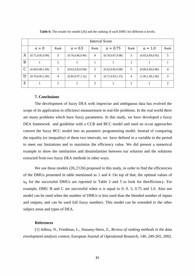
Table 6: The results for model (26) and the ranking of each DMU for different α levels.
Interval Score
α = 0 Rank α = 0.5 Rank α = 0.75 Rank α = 1.0 Rank
A (0.71,0.85,0.99) 3 (0.76,0.86,0.96) 4 (0.76,0.87,0.98) 3 (0.83,0.89,0.95) 5
B 1 1 1 1 1 1 1 1
C (0.60,0.80,1.00) 5 (0.62,0.83,0.94) 5 (0.62,0.85,0.98) 5 (0.86,0.86,0.86) 4
D (0.70,0.85,1.00) 4 (0.85,0.97,1.12) 3 (0.71,0.93,1.25) 4 (1.00,1.00,1.00) 3
E 1 2 1 2 1 2 1 2
7. Conclusions
The development of fuzzy DEA with imprecise and ambiguous data has evolved the
scope of its application to efficienct measurement in real-life problems. In the real world there
are many problems which have fuzzy parameters. In this study, we have developed a fuzzy
DEA framework and guideline with a CCR and BCC model and used an α-cut approachto
convert the fuzzy BCC model into an paramtric programming model. Instead of comparing
the equality (or inequality) of these two intervals, we have defined in a variable in the period
to meet our limitations and to maximize the efficiency value. We did present a numerical
example to show the similarities and dissimilarities between our solution and the solutions
extracted from two fuzzy DEA methods in other ways.
We use these models (20, 21, 26) proposed in this study, in order to find the efficiencies
of the DMUs presented in table mentioned as 1 and 4. On top of that, the optimal values of
u0 for the successful DMUs are reported in Table 2 and 5 to look for theefficiency. For
example, DMU B and C are successful when α is equal to 0, 0. 5, 0.75 and 1.0. Also our
model can be used when the number of DMUs is less used than the blended number of inputs
and outputs, and can be used full fuzzy numbers. This model can be extended to the other
subject areas and types of DEA.
References
[1] Adlera, N., Friedman, L., Sinuany-Stern, Z., Review of ranking methods in the data
envelopment analysis context, European Journal of Operational Research, 140, 249-265, 2002.
82
[2] Bagherzadeh Valami, H., Cost efficiency with triangular fuzzy number input
prices: An application of DEA, Chaos, Solitons and Fractals, 42, 1631-1637, 2009.
[3] Banker, R. D., Thrall, R. M., Estimation of returns to scale using Data
Envelopment Analysis, European Journal of Operational Research, 62, 74-84, 1992.
[4] Bellman, R. E., Zadeh, L. A., Decision-making in a fuzzy environment,
Management Science, 17, 141-164, 1970.
[5] Budak, H., Erpolat, S., Interval data envelopment analysis and an applıcation in
turkish banking sector, European Scientific Journal May, 9(13), 36-50, 2013.
[6] Charnes, A., Clark, T., Cooper, W. W., & Rhodes, E., Measuring the efficiency of
decision-making units, European Journal of Operational Research, 2, 429-444, 1978.
[7] Charnes, A., Cooper, W. W., Golany, B., Seiford, L., Stutz, V. A., Foundations of
data envelopment analysis for Pareto-Koopman efficient empirical production frontiers,
Journal of Econometrics, 30, 91-107, 1985.
[8] Chen, C. B., Klein, C. M., An efficient approach to solving fuzzy MADM problems,
Fuzzy Sets and Systems, 88, 51-67, 1997a.
[9] Chen, C. B., Klein, C. M., A simple approach to ranking a group of aggregated
fuzzy utilities, IEEE Transactions on Systems, Man, and Cybernetics – Part B: Cybernetics,
27, 26-35, 1997b.
[10] Dia, M., A model of fuzzy data envelopment analysis, INFOR, 42(4), 267-279,
2004.
[11] Dubois, D., Prade H., Fuzzy Sets and System: Theory and Application, Academic
Press, New York, 1980.
[12] Goetschel, R., Voxman, W., Elementary Fuzzy calculus, Fuzzy Sets and Systems
18, 31-43, 1986.
[13] Guo, P., Fuzzy data envelopment analysis and its application to locatio
problems, Information Sciences, 179(6), 820-829, 2009.
83
[14] Guo P., Tanaka H., Decision making based on fuzzy data envelopment analysis,
to appear in Intelligent Decision and Policy Making Support Systems (Ruan D. and K. Meer,
Eds.) Springer Berlin / Heidelberg, 39-54, 2008.
[15] Guo, P., Tanaka H., Fuzzy DEA: A perceptual evaluation method, Fuzzy Sets and
Systems, 119(1), 149-160, 2001.
[16] Hatami-Marbini, A., Saati, S., Tavana, M., An ideal-seeking fuzzy data
envelopment analysis framework, Applied Soft Computing, 10(4), 1062-1070, 2010a.
[17] Hatami-Marbini, A., Saati, S., Makui, A., Ideal and anti-Ideal decision making
units: A fuzzy DEA approach, Journal of Industrial Engineering International, 6(10), 31-41,
2010b.
[18] Hatami-Marbini, A., Saati, S., Tavana, M., Data envelopment analysis with fuzzy
parameters: An interactive approach, International Journal of Operations Research and
Information Systems, 2(3), 39-53, 2011.
[19] Hatami-Marbini, A., Tavana, M., Ebrahimi, A., A fully fuzzified data envelopment
analysis model, International Journal of Information and Decision Sciences, 3(3), 252-264,
2011.
[20] Hatami-Marbini, A., Saati, S., Stability of RTS of efficient DMUs in DEA with
fuzzy under fuzzy data, Applied Mathematical Sciences, 3(44), 2157-2166, 2009.
[21] Hatami-Marbini, A., Emrouznejad, A., Tavana, M., A Taxonomy and Review of
the Fuzzy Data Envelopment Analysis Literature: Two Decades in the Making, European
Journal of Operational Research, 214(3), 457-472, 2011.
[22] Hosseinzadeh Lotfi, F., Jahanshahloo, G. R., Alimardani, M., A new approach
for efficiency measures by fuzzy linear programming and Application in Insurance
Organization, Applied Mathematical Sciences, 1(14), 647-663, 2007b.
[23] Hosseinzadeh Lotfi, F., Mansouri, B., The extended data envelopment
analysis/Discriminant analysis approach of fuzzy models, Applied Mathematical
Sciences, 2(30), 1465-1477, 2008.
84
[24] Hosseinzadeh Lotfi, F., Adabitabar Firozja, M., Erfani, V., Efficiency measures
in data envelopment analysis with fuzzy and ordinal data, International Mathematical Forum,
4(20), 995-1006, 2009a.
[25] Hosseinzadeh Lotfi, F., Allahviranloo T., Mozaffari M. R., Gerami J., Basic DEA
models in the full fuzzy position, International Mathematical Forum, 4(20), 983-993, 2009b.
[26] Hosseinzadeh Lotfi, F., Jahanshahloo G. R., Vahidi A. R., Dalirian A., Efficiency
and effectiveness in multi-activity network DEA model with fuzzy data, Applied Mathematical
Sciences, 3(52), 2603-2618, 2009c.
[27] Jahanshahloo, G. R., Soleimani-Damaneh, M., Nasrabadi, E., Measure of
efficiency in DEA with fuzzy input-output levels: A methodology for assessing, ranking and
imposing of weights restrictions, Applied Mathematics and Computation, 156(1), 175-187,
2004a.
[28] Jahanshahloo, G. R., Hosseienzadeh Lotfi, F., Shoja, N., Sanei, M., An alternative
approach for equitable allocation of shared costs by using DEA, Applied Mathematics and
computation, 153(1), 267-274, 2004b.
[29] Jahanshahloo, G. R., Hosseinzade Lotfi, F., Shoja, N., Tohidi, G., Razavian, S.,
Ranking by 𝑙1norm in data envelopment analaysis, Applied Mathematics and Computation,
153(1), 215-224, 2004c.
[30] Jahanshahloo, G. R., Hosseinzadeh Lotfi, F., Shahverdi, R., Adabitabar M.,
Rostam Malkhalifeh M., Sohraiee S., Ranking DMUs by DEA, Chaos, Solitons and Fractals,
39, 2294-2302, 2009b.
[31] Jahanshahloo G. R., Hosseinzadeh Lotfi F., Alimardani Jondabeh M.,
Banihashemi Sh., Lakz aie L., Cost efficiency measurement with certain price on fuzzy data
and application in insurance organization, Applied Mathematical Sciences, 2(1), 1-18, 2008.
[32] Jahanshahloo, G. R., Hosseinzadeh Lotfi, F., Nikoomaram, H., Alimardani, M.,
Using a certain linear ranking function to measure the Malmquist productivity index with
fuzzy data and application in insurance organization, Applied Mathematical Sciences, 1(14),
665-680, 2007a.

85
[33] Jahanshahloo, G. R., Hosseinzadeh Lotfi, F., Adabitabar Firozja, M.,
Allahviranloo, T., Ranking DMUs with Fuzzy Data in DEA, International Journal
Contemporary Mathematical Sciences, 2(5), 203-211, 2007b.
[34] Juan, Y. K., A hybrid approach using data envelopment analysis and case-based
reasoning for housing refurbishment contractors selection and performance improvement,
Expert Systems with Applications, 36(3), 5702-5710, 2009.
[35] Kauffman, A., Gupta, M. M., Introduction to Fuzzy Arithmetic: Theory and
Application, Van Nostrand Reinhold, New York, 1991.
[36] Kao, C., Liu, S. T., Fuzzy efficiency measures in data envelopment analysis,
Fuzzy Set System, 113(3), 427-437, 2000.
[37] Kao, C., Liu, S. T., A mathematical programming approach to fuzzy efficiency
ranking, International Journal of Production Economics, 86, 145-154, 2003.
[38] Lee, H. S., A fuzzy data envelopment analysis model based on dual program,
Conference Proceedings-27th edition of the Annual German Conference on Artificial
Intelligence, 31-39, 2004.
[39] Lee, H. S., Shen, P. D., Chyr, W. L., A fuzzy method for measuring efficiency
under fuzzy environment. Lecture Notes in Computer Science (including subseries Lecture
Notes in Artificial Intelligence and Lecture Notes in Bioinformatics), Melbourne, Australia,
Springer Verlag, Heidelberg, D-69121, Germany, 3682, 343-349, 2005.
[40] Leon, T., Liern, V., Ruiz, J. L., Sirvent, I., A fuzzy mathematical programming
approach to the assessment of efficiency with DEA models, Fuzzy Sets and Systems, 139(2),
407-419, 2003.
[41] Lertworasirikul, S., Fang, S. C., Joines, J. A., Nuttle, H. L. W., Fuzzy data
envelopment analysis (DEA): a possibility approach, Fuzzy Set System, 139(2), 379-394,
2003.
86
[42] Lertworasirikul, S., Fang, S. C., Nuttle, H. L. W., Joines, J. A., Fuzzy BCC model
for data envelopment analysis, Fuzzy Optimization and Decision Making, 2(4), 337-358,
2003.
[43] Liu, Y. P., Gao, X. L., Shen, Z. Y., Product design schemes evaluation based
on fuzzy DEA, Computer Integrated Manufacturing Systems, 13(11), 2099-2104, 2007.
[44] Ma, M., Friedman, M., Kandel, A., A new fuzzy arithmetic, Fuzzy Sets and
Systems, 108, 83-90, 1999.
[45] Majid Zerafat Angiz, L., Mustafa, A., Emrouznejad, A., Ranking efficient
decision-making units in data envelopment analysis using fuzzy concept, Computers &
Industrial Engineering, 8(59), 712-719, 2010.
[46] Moore, R. E., Kearfott, R. B., Cloud, M. J., Introduction to interval analysis,
SIAM, Philadelphia, 2009.
[47] Molavi, F., Aryanezhad, M. B., Shah Alizade, M., An efficiency measurement
model in fuzzy environment, using data envelopment analysis, Journal of Industrial
Engineering International, 1(1), 50-58, 2005.
[48] Noora, A. A., Karami, P., Ranking functions and its application to fuzzy DEA,
International Mathematical Forum, 3(30), 1469-1480, 2008.
[49] Oruç, K. O., Güngör, D., Comparıson of Fuzzy Data Envelopment Analysis
Models: For Interval Data, Journal of Faculty of Economics and Administrative Sciences,
15(2), 417-442, 2010.
[50] Pal, R., Mitra, J., Pal, M. N., Evaluation of relative performance of product
designs: a fuzzy DEA approach to quality function deployment, Journal of the Operations
Research Society of India, 44(4), 322-336, 2007.
[51] Razavi, S. H., Amoozad, H., Zavadskas, E. K., Hashemi, S. S., A Fuzzy Data
Envelopment Analysis Approach based on Parametric Programming, Int. J. Comput.
Commun., 8(4), 594-607, 2013.

87
[52] Saati, S., Memariani, A., Jahanshahloo, G. R., Efficiency analysis and ranking
of DMUs with fuzzy data, Fuzzy Optimization and Decision Making, 1, 255-267, 2002.
[53] Saati, S., Memariani, A., A note on "Measure of efficiency in DEA with fuzzy
input- output levels: A methodology for assessing, ranking and imposing of weights
restrictions" by Jahanshahloo et al, Journal of Science, Islamic Azad University, 16(58/2),
15-18, 2006.
[54] Saati, S., Memariani, A., Reducing weight flexibility in fuzzy DEA, Applied
Mathematics and Computation, 161(2), 611-622, 2005.
[55] Saati, S., Memariani, A., SBM model with fuzzy input-output levels in DEA,
Australian Journal of Basic and Applied Sciences, 3(2), 352-357, 2009.
[56] Sanei, M., Noori, N., Saleh, H., Sensitivity analysis with fuzzy Data in DEA,
Applied Mathematical Sciences, 3(25), 1235-1241, 2009.
[57] Soleimani-Damaneh, M., Fuzzy upper bounds and their applications, Chaos,
Solitons and Fractals, 36, 217-225, 2008.
[58] Soleimani-Damaneh, M., Jahanshahloo, G. R., Abbasbandy, S., Computational
and theoretical pitfalls in some current performance measurement techniques and a new
approach, Applied Mathematics and Computation, 181(2), 1199-1207, 2006.
[59] Wang, C. H., Chuang, C. C, Tsai, C. C., A fuzzy DEA–Neural approach to
measuring design service performance in PCM projects, Automation in Construction, 18,
702-713, 2009b.
[60] Wang X., Kerre, E. E., Reasonable properties for the ordering of fuzzy quantities
(I), Fuzzy Sets and Systems, 118, 375-385, 2001.
[61] Yao, J., Wu, K., Ranking fuzzy numbers based on decomposition principle and
signed distance, Fuzzy Sets and Systems, 116, 275-288, 2000.
[62] Ying-Ming, W., Richard, G., Jian-Bo, Y., Interval efficiency using data
envelopment analysis, Fuzzy Sets and Systems, 153, 347-370, 2005.

88
[63] Zadeh, L. A., Fuzzy sets, Information and Control, 8, 338-353, 1965.
[64] Zhou, S. J., Zhang, Z. D., Li, Y. C., Research of real estate investment risk
evaluation based on fuzzy data envelopment analysis method, Proceedings of the
International Conference on Risk Management and Engineering Management, 444-448, 2008.
[65] Zimmermann, H. J., Fuzzy Set Theory and Its Applications Kluwer, Dordrecht,
1991.