1

AGC 2

1.0 Introduction In the last set of notes, we developed a model of the speed governing mechanism, which is given below:

)ˆ1ˆ(1

ˆ ωΔ−Δ+

=ΔR

PsT

Kx CG

GE (1)

In these notes, we want to extend this model so that it relates the actual mechanical power into the machine (instead of ΔxE), so that we can then examine the relation between the mechanical power into the machine and frequency deviation. What lies between ΔxE, which represents the steam valve, and ΔPM, which is the mechanical power into the synchronous machine? 2.0 Extended model The mechanical power is provided by the prime-mover, otherwise known as the turbine. For

2

nuclear, coal, gas, and combined cycle units, the prime-mover is a steam/gas turbine, and the mechanical power is controlled by a valve. For hydroelectric machines, the prime mover is a hydro-turbine, and the mechanical power is controlled by the water gate. We desire a turbine model which relates the mechanical power control (e.g.: steam valve or water gate) to the mechanical power provided by the turbine. We will be able to illustrate the basic attributes of AGC by using the model for the simplest steam turbine system, the non-reheat turbine,

which responds much like the speed governing system (a single time-constant system). Being a single time-constant system implies that there is only one pole (the characteristic equation has only one root). Thinking in terms of inverse LaPlace transforms, this means that the response to a step-change in valve opening will be exponential (as opposed to oscillatory).

3

Analytically, this means that the relation between the change in valve opening ΔxE and the change in mechanical power into the generator ΔPM is given by:

ET

TM x

sTKP ˆ

1ˆ Δ

+=Δ (2)

Substituting (1) into (2) results in

⎥⎦

⎤⎢⎣

⎡Δ−Δ

++=Δ )ˆ1ˆ(

11ˆ ω

RP

sTK

sTKP C

G

G

T

TM (3)

which is

( )( ) ⎥⎦

⎤⎢⎣

⎡ Δ−Δ++

=Δ ω̂1ˆ

11ˆ

RP

sTsTKKP C

GT

GTM (4)

Let’s assume that KT is chosen so that KTKG=1, then eq. (4) becomes:

( )( ) ⎥⎦

⎤⎢⎣

⎡ Δ−Δ++

=Δ ω̂1ˆ

111ˆ

RP

sTsTP C

GTM (5)

A block diagram representing eq. (5) is given in Fig. 1.

4

R1

Σ ( )( )sTsT GT ++ 11

1

-

+

ΔPC

Δω

ΔPM

Fig. 1

3.0 Mechanical power and frequency Let’s expand (5) so that

( )( ) ( )( ) RsTsTsTsTPP

GTGT

CM

ω̂111

11

ˆˆ Δ++

−++

Δ=Δ (6)

Consider a step-change in power of ΔPC and in frequency of Δω, which in the LaPlace domain is:

sω

ωΔ

=Δ ˆ (7a)

sPP C

CΔ

=Δ ˆ (7b) Substitution of (7a) and (7b) into (6) results in:

5

( )( ) ( )( ) RsTsTssTsTsPP

GTGT

CM

11111

ˆ++

Δ−

++Δ

=Δω

(8) One easy way to examine eq. (8) is to consider ΔPM(t) for very large values of t, i.e., for steady-state. To do this, consider that the variable ΔPM in eq. (8) is a LaPlace variable. To consider the corresponding time-domain variable under the steady-state, we may employ the final value theorem, which is:

)(ˆlim)(lim0

sfstfst →∞→

= (9) Applying eq. (9) to eq. (8), we get:

( )( ) ( )( )

( )( ) ( )( )

RP

RsTsTsTsTP

RsTsTss

sTsTsPs

PstPP

C

GTGT

Cs

GTGT

Cs

MsMtM

ω

ω

ω

Δ−Δ=

⎭⎬⎫

⎩⎨⎧

++Δ

−++

Δ=

⎭⎬⎫

⎩⎨⎧

++Δ

−++

Δ=

Δ=Δ=Δ

→

→

→∞→

11111

lim

11111

lim

ˆlim)(lim

0

0

0

(10)

6

Therefore,

RPP CM

ωΔ−Δ=Δ (11)

Make sure that you understand that in eq. (11), ΔPM, ΔPC, and Δω are • Time-domain variables (not LaPlace variables) • Steady-state values of the time-domain variables (the values after you wait along time)

Because we developed eq. (11) assuming a step-change in frequency, you might be misled into thinking that the frequency change is the initiating change that causes the change in mechanical power ΔPM. However, recall Fig. 3 of AGC1 notes, repeated below for convenience as Fig. 2 in these notes.

7

Fig. 2

The frequency change expressed by Δω in eq. (11) is the frequency deviation at the end of the simulation. The ΔPM in eq. (11), associated with Fig. 2, is • not the amount of generation that was outaged, • but rather the amount of generation increased at a certain generator in response to the generation outage.

So ΔPM and Δω are the conditions that can be observed at the end of a transient initiated by a load-generation imbalance. They are not

8

conditions inherent to the synchronous generator, but rather conditions that result from the action of the primary governing control. In other words, the primary governing control will operate (in response to some frequency deviation caused by a load-generation imbalance) to change the generation level by ΔPM and leave a steady-state frequency deviation of Δω. To obtain a plot of PM vs. ω for a certain setting of PC=PC1, we assume that the local behavior as characterized by eq. (11) can be extrapolated to a larger domain:

RPP CM

01

ωω −−=−

Such a plot appears in Fig. 3.

9

PM

ω

RPM

ωΔ−=Δ

Slope=-1/R

PC1

ω0

Δω

ΔPM

Fig. 3

The plot, therefore, provides an indication of what happens to the mechanical power PM, and the frequency ω, following a disturbance from this pre-disturbance condition for which PM=PC1 and ω= ω0. If we were to change the generation set point to PC=PC2, then the entire characteristic moves to the right, as shown in Fig. 4.

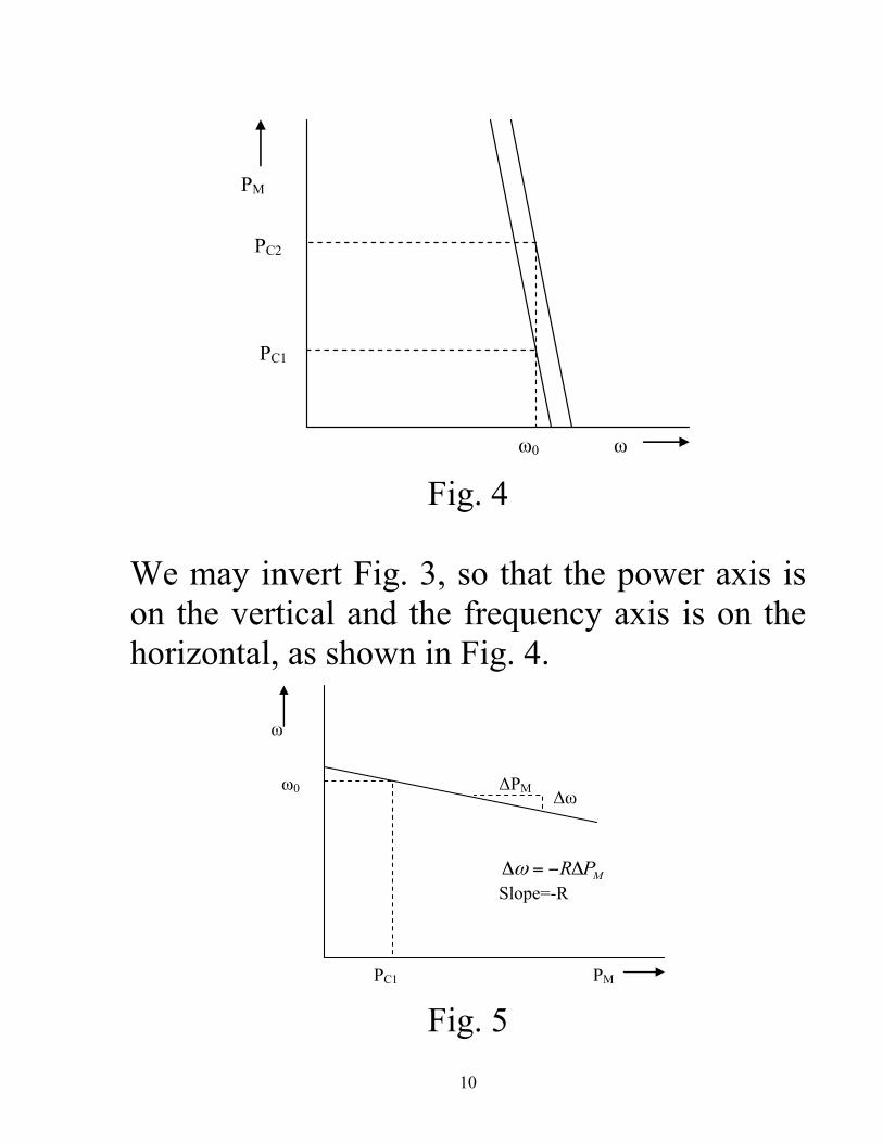
10

PM

ω

PC1

ω0

PC2

Fig. 4

We may invert Fig. 3, so that the power axis is on the vertical and the frequency axis is on the horizontal, as shown in Fig. 4.

PM

ω

MPRΔ−=ΔωSlope=-R

PC1

ω0 Δω ΔPM

Fig. 5

11

Fig. 6 illustrates what happens when we change the generation set point from PC=PC1 to PC=PC2.

PM

ω

PC1

ω0

PC2 Fig. 6

It is conventional to illustrate the relationship of frequency ω and mechanical power PM as in Figs. 5 and 6, rather than Figs. 3 and 4. From Figs. 5 and 6, we obtain the terminology “droop,” in that the primary control system acts in such a way so that the resulting frequency “droops” with increasing mechanical power. The R constant, previously called the regulation constant, is also referred to as the droop setting.

12

4.0 Units Recall eq. (11), repeated here for convenience.

RPP CM

ωΔ−Δ=Δ (11)

With no change to the generation set point, i.e., ΔPC=0, then

RPM

ωΔ−=Δ (12)

where we see that

MPR

ΔΔ

−=ω

(13) We see then that the units of R must be (rad/sec)/MW. A more common way of specifying R is in per-unit; we convert to per-unit the top and bottom of eq. (13), so that:

Mpu

pu

rMpu PSPR

Δ

Δ−=

ΔΔ

−=ωωω

// 0

(14) where ω0=377 and Sr is the three-phase MVA rating of the machine. When specified this way, R relates fractional changes in ω to fractional changes in PM.

13

It is also useful to note that

pupu fff

ff

Δ=Δ

=Δ

=Δ

=Δ000 2

2ππ

ωω

ω (15) Thus, we see that per-unit frequency is the same independent of whether it is computed using rad/sec or Hz, as long as the proper base is used. Therefore, eq. (14) can be expressed as

Mpu

pu

Mpu

pupu P

fP

RΔ

Δ−=

Δ

Δ−=

ω (16)

5.0 Example Consider a 2-unit system, with data as follows:

Gen A: SRA=100 MVA, RpuA=0.05 Gen B: SRB=200 MVA, RpuB=0.05

The load increases, with appropriate primary speed control (but no secondary control) so that the steady-state frequency deviation is 0.01 Hz. What are ΔPA and ΔPB?

14

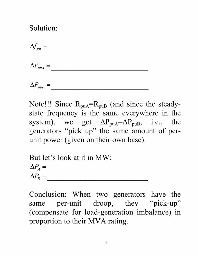
Solution:

=Δ puf __________________________

=Δ puAP _________________________

=Δ puBP _________________________ Note!!! Since RpuA=RpuB (and since the steady-state frequency is the same everywhere in the system), we get ΔPpuA=ΔPpuB, i.e., the generators “pick up” the same amount of per-unit power (given on their own base). But let’s look at it in MW:

=Δ AP __________________________ =Δ BP __________________________

Conclusion: When two generators have the same per-unit droop, they “pick-up” (compensate for load-generation imbalance) in proportion to their MVA rating.

15

In North America, droop constants for most units are set at about 0.05 (5%). 6.0 Multi-machine case Now let’s consider a general multi-machine system having K generators. From eq. (16), for a load change of ΔP MW, the ith generator will respond according to:

60/60/ f

RSP

SPfR

pui

RiMi

RiMipui

Δ−=Δ⇒

ΔΔ

−= (17) The total change in generation will equal ΔP, so:

60...

1

1 fRS

RS

PKpu

RK

pu

R Δ

⎥⎥⎦

⎤

⎢⎢⎣

⎡++−=Δ (18)

Solving for Δf results in

⎥⎥⎦

⎤

⎢⎢⎣

⎡++

Δ−=

Δ

Kpu

RK

pu

R

RS

RS

Pf

...60

1

1 (19)

16

Substitute eq. (19) back into eq. (17) to get:

⎥⎥⎦

⎤

⎢⎢⎣

⎡++

Δ=

Δ−=Δ

Kpu

RK

pu

Rpui

Ri

pui

RiMi

RS

RS

PRSf

RSP

...60

1

1 (20)

If all units have the same per-unit droop constant, i.e., Rpui=R1pu=…=RKpu, then eq. (20) becomes:

[ ]RKR

Ri

pui

RiMi SS

PSfRSP

++Δ

=Δ−

=Δ...60 1

(21) which generalizes our earlier conclusion for the two-machine system that units “pick up” in proportion to their MVA ratings. This conclusion should drive the way an engineer performs contingency analysis of generator outages, i.e., one should redistribute the lost generation to the remaining generators in proportion to their MVA rating, as given by eq. (21).