Agenda

Review Exam ISampling

Start Probabilities

Exam I

• Ex1 Written + Ex1 MC = raw score• (Raw score / 86) = raw percent• Raw percent + 6 = final recorded = Exam1%

• Distribution 5 F, 5D, 6C, 8B, 3A• Mean = 76, Median = 78

Distribution of Exam 1 Scores

Short Essay questions

• Pillars + Study• Nominal vs. Operational definition • Validity vs. Reliability• Anonymity vs. Confidentiality

Why Draw A Sample?

• Why not just the get the whole enchilada? – Pragmatic reasons– The true population is typically “unknowable”

• When done right, a small proportion of the population works just fine…

Types of Sampling

• Probability Sampling– Based on the principles of probability theory– Elements of the population have some known

probability (typically equal odds) of selection• Non-probability sampling

– Elements in the population have unknown odds of selection

• Make it very difficult to generalize findings back to the population of interest

Non-Probability Sampling

• Reliance on available subjects• Purposive/judgmental sampling• Snowball sampling• Quota sampling • Informants

Probability Sampling

• Terminology– Element – Population– Sample– Sampling Frame– Parameter vs. Statistic

Probability Sampling

• Advantages– Avoids both conscious and unconscious bias– By using probability theory, we can judge the

accuracy of our findings• There is ALWAYS ERROR in any sample• No sample perfectly reflects the entire population • Key issue = How much error is likely in our specific

sample?

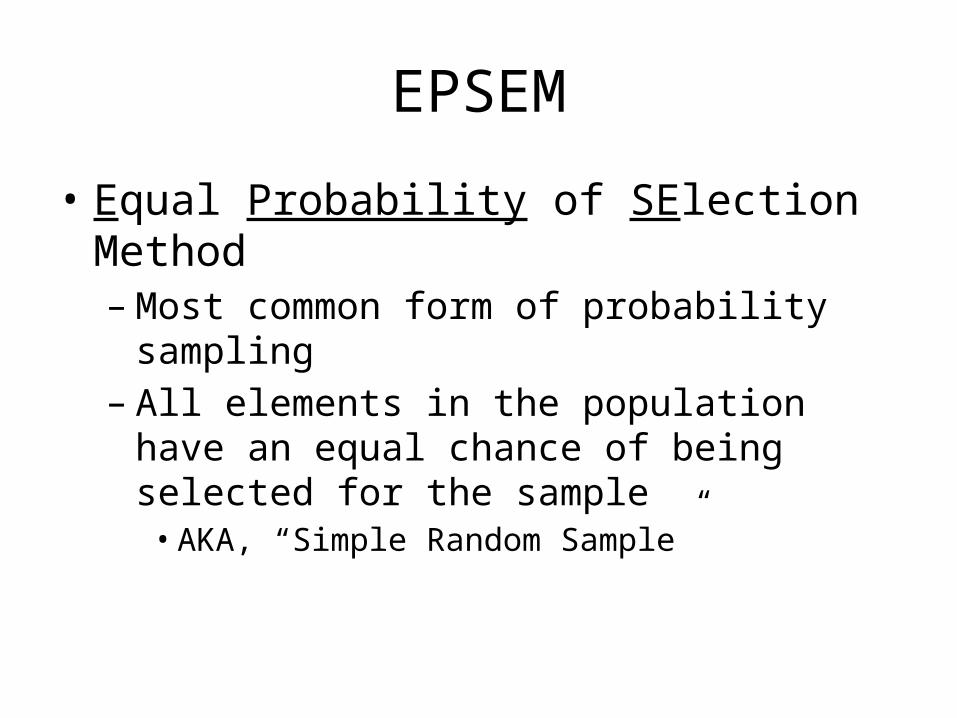
EPSEM

• Equal Probability of SElection Method– Most common form of probability sampling– All elements in the population have an equal

chance of being selected for the sample• AKA, “Simple Random Sample”

Probability Theory

• A branch of mathematics that allows us to gauge how well our sample statistics reflect the true population parameters.

• Based on HYPOTHETICAL distributions – What would happen if we took an infinite number

of unbiased (EPSEM) samples from a population and plotted the results?

• Some “weird” findings just by chance (large errors)• Findings closer to the true parameter more likely (small

errors)

Probability Theory II

• Hypothetical distributions are called:– Sampling distributions– Probability distributions

• Sampling/probability distributions exist for any kind of sample outcome you can imagine– Percent, mean, mean difference… – ALL OF THEM PRODUCE “KNOWN” ESTIMATES OF

ERROR • How sample outcomes will be distributed around the true

population parameter

Probability Theory III

• Standard deviation = how far a case typically falls from the mean of a distribution – Measure of dispersion

• Standard error– The standard deviation of a sampling/probability distribution

• KEY POINT: standard deviations of a sampling distribution always contain the same percent of sample outcomes

– +/-1 Standard Error contains 68% of outcomes– +/- 1.96 Standard Errors contains 95% of outcomes– +/- 2.58 Standard Errors contains 99% of outcomes

Probability Theory IV

• The sampling distribution therefore tells us generally how sampling error is distributed around a population parameter– 68% of sample outcomes will be within one standard error of

the true population parameterOR– There a 68% chance that a particular sample outcome falls

within one standard error of the population parameter– There a 95% chance that a particular sample outcome falls

within two standard errors (1.96) of the population parameter

• This logic is what we use to calculate our specific error

.95 means that this window contains 95% of all

sample outcomes—OR, there is a 95% chance of getting an outcome in this window

0.95

-1.96 1.96

.025 .025

Standard Errors

Sampling Distribution

Getting estimates of error for a specific sample outcome

• The error for a particular sample depends upon…• Sample Size larger samples = less error• Dispersion/homogeneity in the sample greater

homogeneity = less error

Estimation

• Point Estimate: Value of a sample statistic used to estimate a

population parameter• Confidence Interval: A range of values around the point

estimate

Confidence IntervalPoint Estimate

Confidence Limit (Lower)

Confidence Limit (Upper)

.58.546 .614

Confidence Intervals

– We can calculate a “confidence interval” around a sample finding

• We can be 95%, 99% (or whatever) certain that some sample finding is within +/- points/units

– We are 99% confident that 77%, +/- 4 %, of UMD students would car splash professor Maahs with a puddle if they drove by and had the opportunity

» OR, We are 99% sure that between 73% and 81% of UMD students….

– Based on our sample findings, we are 95% confident that average age of Duluth homeowners is between 36.5 and 41.5 years old

» Or, 39 years old, +/- 2.5 years

Calculating a confidence interval

• Step 1: Choose a confidence level:– 95% confident means going out +/- 1.96 standard errors– 99% confident means going out +/- 2.58 standard errors – How many standard errors would you have to go out to

be 68% confident?

• KEY: Extend logic from what would happen with infinite number of samples to “odds of obtaining a sample finding within 1, 1.96, or 2.58 standard errors of population parameter”

Calculating a confidence interval

• Step 2: figuring out what a standard error is “worth” for your situation – Sample size (N)– Some estimate of dispersion – There are formulas for every situation

• Babbie The “Binomial” – Used for agree/disagree survey questions (%

agree)

Example

• CNN Poll (CNN.com; Feb 20, 2009): Slight majority thinks stimulus package will improve economy

• “The White House's economic stimulus plan isn't a surefire winner with the American public, but a majority does think the recovery plan will help. According to a new poll, fifty-three percent said the plan will improve economic conditions, while 44 percent said it won't stimulate the economy.”

• “On an individual level, there was less hope for improvement. According to the poll, 67 percent said it would not help them personally.”

• “The Poll was conducted Wednesday and Thursday (Feb 18-19, 2009), with 1,046 people questioned by telephone. The survey's sampling error is plus or minus 3 percentage points.”

Estimation– POINT ESTIMATES

• (another way of saying sample statistics)

– CONFIDENCE INTERVAL• a.k.a. “MARGIN OF ERROR”• Indicates that over the long run,

95 percent of the time, the true pop. value will fall within a range of +/- 3

“…but a majority does think the recovery plan will help, according to a new poll. Fifty-three percent said the plan will improve economic conditions, while 44 percent said it won't stimulate the economy.

…. The Poll was conducted Wednesday and Thursday (Feb 18-19, 2009), with 1,046 people questioned by telephone. The survey's sampling error is plus or minus 3 percentage points.

Confidence Intervals for Proportions

• Sample point estimate (convert % to a proportion): – “Fifty-three percent said the plan will improve economic

conditions…”– 0.53

• Sample size (N) = 1,046• Formula in Babbie (p.217)

– Numerator = (your proportion) (1- proportion)– 95% confidence level (replicating results from article)

Example 1: Estimate for the economic recovery poll

• p = .53 (53% think it will help)• 95% confidence interval = 1.96 standard errors• N = 1046 (sample size) • What happens when we…

– Recalculate for N = 10,000– Back to original, but change confidence level to 99%