Carnegie Mellon UniversityResearch Showcase @ CMU

Department of Chemical Engineering Carnegie Institute of Technology

11-2014

Air Separation with Cryogenic Energy Storage:Optimal Scheduling Considering Electric Energyand Reserve MarketsQi ZhangCarnegie Mellon University

Clara F. HeubergerAachen University of Technology

Ignacio E. GrossmannCarnegie Mellon University, grossmann@cmu.edu

Arul SundaramoorthyPraxair

Jose M. PintoPraxair

Follow this and additional works at: http://repository.cmu.edu/cheme

Part of the Chemical Engineering Commons

This Conference Proceeding is brought to you for free and open access by the Carnegie Institute of Technology at Research Showcase @ CMU. It hasbeen accepted for inclusion in Department of Chemical Engineering by an authorized administrator of Research Showcase @ CMU. For moreinformation, please contact research-showcase@andrew.cmu.edu.

Air Separation with Cryogenic Energy Storage: Optimal SchedulingConsidering Electric Energy and Reserve Markets

Qi Zhanga, Clara F. Heubergerb, Ignacio E. Grossmanna,∗, Arul Sundaramoorthyc, Jose M. Pintod

aCenter for Advanced Process Decision-making, Department of Chemical Engineering, Carnegie Mellon University,Pittsburgh, PA 15213, USA

bFaculty of Mechanical Engineering, RWTH Aachen University, 52056 Aachen, GermanycPraxair, Inc., Business and Supply Chain Optimization R&D, Tonawanda, NY 14150, USAdPraxair, Inc., Business and Supply Chain Optimization R&D, Danbury, CT 06810, USA

Abstract

The concept of cryogenic energy storage (CES) is to store energy in the form of liquid gas and vaporize

it when needed to drive a turbine. Although CES on an industrial scale is a relatively new approach,

the technology is well-known and essentially part of any air separation unit (ASU) that utilizes cryogenic

separation. In this work, we assess the operational benefits of adding CES to an existing air separation plant.

We investigate three new potential opportunities: (1) increasing the plant’s flexibility for load shifting, (2)

storing purchased energy and selling it back to the market during higher-price periods, (3) creating additional

revenue by providing operating reserve capacity. We develop a mixed-integer linear programming (MILP)

scheduling model and apply a robust optimization approach to model the uncertainty in reserve demand.

The proposed model is applied to an industrial case study, which shows significant potential economic

benefits.

Keywords: Air separation, cryogenic energy storage, production scheduling, electricity markets,

mixed-integer linear programming, robust optimization

Introduction

In light of high fluctuations in electricity demand and increasing penetration of intermittent renewable

energy into the electricity supply mix, energy storage is considered a key element in enhancing the efficiency

∗Corresponding authorEmail address: grossmann@cmu.edu (Ignacio E. Grossmann)

and reliability of the power grid [1, 2]. By storing energy during off-peak and releasing it during on-

peak hours, the need for further peak generation capacity is reduced, which averts additional capital and

operating costs. Properly located storage can reduce congestion in the transmission network; moreover, it is

well-suited for providing ancillary services to offset real-time differences between supply and demand. From

an electricity consumer’s point of view, energy storage can be effectively used for Demand Side Management

purposes, e.g. reducing costs by shifting load from high-price to low-price periods [3].

The concept of cryogenic energy storage (CES) is to store energy in the form of liquefied gas. When

energy is needed at a later time, the liquid gas is pumped to high pressure and vaporized, e.g. by using

low-grade heat; the high-pressure gas can then be used to drive a turbine to generate electricity. The

CES technology is being pioneered in the UK [4, 5] where the company Highview Power Storage has been

running a liquid air energy storage (LAES) pilot plant since 2011 and is currently building a higher-capacity

pre-commercial demonstration plant, which is planned to go online in 2015 (www.highview-power.com).

Different applications of CES have been proposed, e.g. integrating it with oxy-fuel combustion and carbon

capture [6]. However, studies of CES systems at an operational level are scarce, although essential since the

true benefit of CES can only be assessed by accounting for electricity market dynamics.

Interestingly, although CES on an industrial scale is a relatively new approach, the technology used for

CES is well-known and essentially part of every air separation unit (ASU) that utilizes cryogenic separation.

In cryogenic air separation, air is separated into its individual components at low temperatures, and typically,

large amounts of oxygen and nitrogen are liquefied to be transported to customers via tanker trucks. Before

being picked up by the trucks, the liquid products are stored in large tanks. Hence, by simply adding a few

pieces of equipment, namely pump, heat exchanger, and turbine, one would be able to vaporize the stored

liquid products and generate electricity, which by definition makes it a CES system.

The question that we raise and try to answer in this work is what are the potential operational benefits

of an air separation plant with added CES capability. Here, we see three immediate opportunities for such

an integrated ASU-CES system: (1) In general, an ASU has a limited range of oxygen to nitrogen ratio

at which it can efficiently operate. This often leads to overproduction of one product, which is typically

2

vented and therefore wasted. With CES, instead of venting overproduced products, we can store them

and recover energy from them to increase the plant’s flexibility for load shifting. (2) Power generated from

the CES system can be sold to the electricity market. This may be an important new source of revenue,

especially in times when the demand for LO2 and LN2 is low and the air separation plant is therefore

underutilized. (3) Similarly, the plant can also participate in the ancillary services market by providing

operating reserve capacities which can be dispatched upon request. Operating reserves are required when

the real-time electricity demand in the grid is higher than the supply, e.g. due to unexpected load increase

or generator failures.

Load shifting is a typical Demand Response (DR) activity, which generally refers to electricity consumers

intentionally modifying their power consumption profiles [7, 8] in order to take advantage of time-sensitive

electricity prices and other market incentives. This does not only benefit the electricity consumers but

also helps balancing supply and demand in the grid. Overviews of existing DR strategies as well as the

corresponding benefits and challenges are provided in various review and perspective papers [9, 10, 11]. The

high potential impact of large industrial electricity consumers, such as air separation plants, participating

in DR is widely acknowledged [12, 13, 14] and has been the focus of increased research and development

efforts in recent years. One of the most prominent success stories in industrial DR is the one by Alcoa, which

uses the operational flexibility of its aluminum smelting facilities to provide ancillary services through which

the company is achieving large economic benefits [15]. Systematic optimization approaches for DR have

been proposed for various other industrial power-intensive processes such as steelmaking [16, 17], cement

production [18, 19], and electrolysis [20]. In particular, to a certain extent, this work is motivated by previous

works [21, 22, 23] that have shown the large potential benefits of DR for air separation plants.

With its energy storage capability, an ASU-CES system does not only consume but can also generate

electricity. As such, it has the opportunity to gain additional benefits by participating as a supplier in

electricity markets. Just like consumers, suppliers as well are exposed to volatility in electricity price. The

scheduling of power producers’ operations in the short-term electricity market is a classic problem and has

been widely addressed by the power systems engineering community, in particular for hydro [24, 25] and

3

thermal [26, 27, 28] power producers. Similarly, Mitra et al. [29] optimize the scheduling of a combined heat

and power plant that interacts with the electricity market as well as a chemical plant to which it supplies

electricity and steam.

In general, there are two different forms in which electricity can be traded in modern electricity markets:

energy and ancillary services [30]. Energy is simply what we know as electric energy or power, whereas

ancillary services are backup capacities that are called upon when real-time electricity supply and demand in

the grid do not match, e.g. due to equipment failures or sudden load changes. Ancillary services are therefore

crucial for the stability of the power grid, and depending on how fast these capacities can be dispatched,

they are categorized as operating reserve (response within minutes) or regulation (within seconds) service.

Since power drawn from a CES is generated via a gas turbine, the system can react within minutes and is

thus capable of providing operating reserve. Previous works have focused on the problem of deciding how

much reserve is required in the grid [31, 32, 33]. There are very few references in the literature that address

the problem from a reserve provider’s standpoint, who has to decide on the optimal amount of reserve

capacity to sell. The main challenge here lies in the uncertain nature of the reserve demand. Since demand

for operating reserve occurs due to unexpected events, the reserve provider does not know in advance what

amount and, above all, when reserve service has to be dispatched. Vujanic et al. [34] address this issue with

a robust optimization approach which has been applied to a cement plant that provides reserve by shifting

load. Here, the uncertainty lies in the time of required reserve dispatch and is assumed to affect the start

times of the scheduled tasks.

The objective of this work is to investigate at an operational level whether adding CES capability to an

existing air separation plant can be beneficial. This can be seen as an initial economic assessment of a new

technology, and to the best of our knowledge, the problem as such has not been addressed in the literature

before. The main contributions of this work are the following:

� We develop a mixed-integer linear programming (MILP) model for the scheduling of an integrated

ASU-CES plant.

� To account for the uncertainty in reserve demand, we apply a robust optimization approach that yields

4

solutions that guarantee feasibility for any realization of the uncertainty within the uncertainty set.

At the same time, the form of the uncertainty set provides the flexibility of adjusting the level of

conservatism in the problem.

� We apply the proposed model to a real-world industrial case study provided by Praxair. The corre-

sponding sensitivity analysis shows the potential benefit as a function of plant utilization and CES

efficiency.

The remainder of this paper is organized as follows. In the next section, the problem statement is

presented. We then develop the MILP scheduling model for the integrated ASU-CES plant, and derive the

robust model that allows the optimization of selling reserve capacities. The results of the industrial case

study are shown before we close with a summary of the main results and some concluding remarks.

Problem Statement

Consider that to an existing air separation plant that consumes air and electricity to produce gaseous

oxygen (GO2), gaseous nitrogen (GN2) as well as liquid oxygen (LO2), liquid nitrogen (LN2), and liquid

argon (LAr), a CES system is added that can generate electricity by vaporizing LO2 or LN2. LAr will not

be used for CES because it is produced in much lower quantities and has a considerably higher market value

than LO2 and LN2; thus, it can be assumed to be always more profitable to sell all LAr that is produced.

The power drawn from the CES can be used internally to make more products, or it can be sold to the

electric energy market. Furthermore, operating reserve capacity can be provided and sold to the reserve

market.

The plant has to satisfy product demand, which can be specified on an hourly basis. Gaseous product

customers are connected to the plant via pipelines. We assume that there is no capacity for storing GO2 and

GN2. However, there is the possibility of vaporizing LO2 and LN2 to feed the pipelines in case GO2 and GN2

production from the ASU alone is too low to satisfy the demand; in the air separation industry, this process

is referred to as driox. LO2 and LN2 are stored in inventory tanks and distributed to the customers when

5

required. The liquid product demand is considered to be the amount needed to be drawn from the tanks

and shipped to the customers. Alternatively, liquid products can be purchased from third-party suppliers.

We assume that a forecast for the electricity and reserve prices is available on an hourly basis, and that

the scheduling decisions do not influence those prices. The demand for operating reserve is not known in

advance; however, the requested amount of power to be dispatched cannot exceed the committed reserve

capacity.

The objective is to find a schedule for the integrated ASU-CES plant over a given scheduling horizon

(typically a week) that minimizes the total operating cost minus the revenue from selling power and reserve

capacity. The problem is to determine for every hour of the scheduling horizon:

� the mode of operation for the ASU,

� the production level of each product,

� the amount of liquid products stored,

� the amount of liquid products used for driox,

� the amount of liquid products purchased,

� the amount of power purchased from the electricity market,

� the amount of power sold to the electricity market,

� and the reserve capacity provided.

Integrated ASU-CES Model

The scheduling problem stated in the previous section can be formulated as an MILP. In the following,

the mathematical formulation of the MILP model is presented. Note that all continuous variables in this

model are constrained to be nonnegative. A list of indices, sets, parameters, and variables is given in the

Nomenclature section.

6

We apply a discrete-time framework in which the time horizon is divided into time periods of equal

length, ∆t. The notation for the time discretization is such that time period t starts at time point t− 1 and

ends at time point t. The scheduling horizon is defined by the set of time periods T = {1,2, . . . , tf}. T is a

subset of T = {−θu + 1,−θu + 2, . . . ,0,1, . . . , tf} which also includes time periods in the past that are used in

some constraints involving multiple time periods. The common-grid representation is illustrated in Figure

1.

Figure 2 depicts the mass and power flows in an integrated ASU-CES system interacting with gas and

liquid customers as well as electricity markets. Note that reserve market participation is not considered in

the model described in this section but will be addressed in detail in the next section. In the following, we

first present the mass and energy balance constraints before elaborating on how the air separation process

is modeled.

Mass Balances

The ASU produces liquid and gaseous products, which are defined by the product sets I and I, respec-

tively, i.e. I = {LO2, LN2, LAr} and I = {GO2,GN2}. I = {LO2, LN2} is the set of liquid products that

can be stored for CES. Eqs. (1)–(3) state the mass balance equations for the liquid products, whereas mass

balances for the gaseous products are given in Eq. (4).

Eq. (1a) states that the LO2 and LN2 produced in the ASU in each time period, denoted by PDit, are

either stored as liquid product inventory or CES inventory. As expressed in Eq. (1b), for liquid products

not used for CES, which in this case is only LAr, there is no flow into the CES tank.

PDit = FLit + FLit ∀ i ∈ I , t ∈ T (1a)

PDit = FLit ∀ i ∈ I ∖ I , t ∈ T (1b)

As stated in Eq. (2a), the liquid product inventory level at time t is the inventory level at time t−1 plus

the flow into the inventory tank during time period t, FLit, minus the amount drawn from the tank and

shipped out, SLit, and the amount consumed by the driox process, V Pit, during time period t. Eq. (2b)

7

sets lower and upper bounds on the inventory levels while Eq. (2c) states that the liquid demand, Dit, has

to be satisfied by the sum of the amount drawn from the inventory tank and the amount purchased, PCit.

IVit = IVi,t−1 + FLit − SLit − V Pit ∀ i ∈ I , t ∈ T (2a)

IV li ≤ IVit ≤ IVui ∀ i ∈ I , t ∈ T (2b)

SLit + PCit =Dit ∀ i ∈ I , t ∈ T (2c)

Change in the CES inventory level, IV t, over time is described by the following constraints:

FLag

t =∑i∈IFLit ∀ t ∈ T (3a)

IV t = IV t−1 + FLag

t −EDt

η∀ t ∈ T (3b)

IVl≤ IV t ≤ IV

u∀ t ∈ T (3c)

where we aggregate the flows into the CES tank, FLit, assuming that LO2 and LN2 will yield the same

amount of energy when vaporized and sent through a turbine. This is a fairly reasonable assumption since

the two gases have similar heat capacities and heats of vaporization. As given by Eq. (3b), the resulting

aggregate flow, FLag

t , minus the amount of liquid used for electricity generation, EDt/η, constitute the

change in the CES inventory level over time period t. Here, EDt denotes the electricity discharged in time

period t, and η is the power generation efficiency given in units of power per mass. Eq. (3c) sets bounds for

the CES inventory level.

The following equation states the mass balance for the gaseous products:

PDit + ρi′V Pi′t =Dit + V Tit ∀ i ∈ I , i′ = fV P (i), t ∈ T (4)

where V Tit is the gas vented due to overproduction. With the variable V Pit, we account for the liquid

products sent to driox to be vaporized. Here, fV P ∶ I → I denotes the unique mapping of gaseous to liquid

8

products, e.g. fV P (GO2) = LO2.

Energy Balances

As stated in Eq. (5a), the amount of power discharged from the CES in time period t, EDt, can be used

internally in the ASU (EDint ) or sold to the electric energy market (EDen

t ). Again, note that operating

reserve (EDret ) is not considered at this point. EDt is limited by an upper bound, EDu, given in Eq.

(5b), which in practice depends on the size of the turbine. In Eq. (5c), ECt denotes the amount of power

consumed by the ASU in time period t, which consists of EDint and EPt, the amount of power purchased

from the energy market.

EDt = EDint +EDen

t ∀ t ∈ T (5a)

EDt ≤ EDu

∀ t ∈ T (5b)

ECt = EDint +EPt ∀ t ∈ T (5c)

ASU Model

Cryogenic air separation is a highly integrated process; thus, detailed models of ASUs are extremely

complex. In order to retain computational tractability when solving the scheduling problem, we use a

surrogate model to represent the ASU. As proposed by Mitra et al. [23], we assume that the ASU can

operate in different operating modes. Each mode corresponds to a particular configuration or state of the

plant, e.g. “off”, “start-up”, or “production”. In the proposed model, each mode is defined by a Convex

Region Surrogate (CRS) model [35], in which the feasible region is approximated by a union of convex

subregions in the form of polytopes with a linear power consumption correlation for each subregion. Figure

3 shows an illustrative example with two CRS models in a two-dimensional product space. This can be

interpreted as the feasible product region of an ASU that can operate in two modes. The feasible region

corresponding to Mode 1 is represented by one single convex region, whereas the Mode 2 surrogate model

consists of two convex subregions, 2a and 2b.

9

Physically, at any point in time, the ASU can only run in one operating mode. In an operating mode,

the operating point has to lie in either one of the convex regions. Any point in a convex region can be

represented as a convex combination of the vertices of the polytope. These relationships can be expressed

by the following nested disjunction:

⋁m∈M

⎡⎢⎢⎢⎢⎢⎢⎢⎢⎢⎢⎢⎢⎢⎢⎢⎢⎢⎢⎢⎢⎢⎢⎢⎢⎢⎢⎢⎢⎢⎢⎣

⋁r∈Rm

Ymt

⎛⎜⎜⎜⎜⎜⎜⎜⎜⎜⎜⎜⎜⎜⎜⎜⎜⎜⎜⎜⎜⎜⎝

Y mrt

PDit = ∑j∈Jmr

λmrjt vmrji ∀ i

∑j∈Jmr

λmrjt = 1

0 ≤ λmrjt ≤ 1 ∀ j ∈ Jmr

ECt = δmr +∑iγmri PDit

⎞⎟⎟⎟⎟⎟⎟⎟⎟⎟⎟⎟⎟⎟⎟⎟⎟⎟⎟⎟⎟⎟⎠

⎤⎥⎥⎥⎥⎥⎥⎥⎥⎥⎥⎥⎥⎥⎥⎥⎥⎥⎥⎥⎥⎥⎥⎥⎥⎥⎥⎥⎥⎥⎥⎦

∀ t ∈ T

∨

m∈MYmt ∀ t ∈ T

Ymt⇔ ∨r∈Rm

Y mrt ∀m ∈M, t ∈ T

Ymt ∈ {true, false} ∀m ∈M, t ∈ T

Y mrt ∈ {true, false} ∀m ∈M, r ∈ Rm, t ∈ T

(6)

where M is the set of all operating modes, Rm is the set of convex regions associated with mode m, and

Jmr is the set of vertices of region r ∈ Rm. Ymt and Y mrt are boolean variables. Ymt is true if mode m is

selected in time period t, whereas Y mrt is true if region r ∈ Rm is selected in time period t. The amount of

product i produced, PDit, is expressed as a convex combination of the corresponding vertices, vmrji, while

the amount of power consumed, ECt, is a linear function of PDit with a constant δmr and coefficients γmri

specific to the selected region.

By applying the hull reformulation [36], the disjunction given by Eq. (6) can be transformed into the

10

following MILP constraints:

PDit =∑m

∑r∈Rm

PDmrit ∀ i, t ∈ T (7a)

PDmrit = ∑j∈Jmr

λmrjt vmrji ∀m, r ∈ Rm, i, t ∈ T (7b)

∑j∈Jmr

λmrjt = ymrt ∀m, r ∈ Rm, t ∈ T (7c)

ECt =∑m

∑r∈Rm

(δmr ymrt +∑i

γmri PDmrit) ∀ t ∈ T (7d)

ymt = ∑r∈Rm

ymrt ∀m, t ∈ T (7e)

∑m

ymt = 1 ∀ t ∈ T (7f)

where ymt and ymrt are binary variables, and PDmrit are disaggregated variables of which only one is

nonzero for each time period t.

Transition Constraints

A transition occurs when the system changes from one operating point to another. We assume that

the transition between different operating points in the same mode can be completed within a time frame

much shorter than one time period. Hence, the model allows transitions from any operating point in one

time period to any other operating point in the same mode in the immediate next time period. However,

constraints have to be imposed on transitions between different modes.

Eqs. (8)–(10), which model the transition constraints, are adopted from Mitra et al. [23, 29]. Here,

zmm′t is a binary variable which is 1 if and only if the plant switches from mode m to mode m′ at time t,

which is enforced by the following constraint:

∑

m′∈TRfm

zm′m,t−1 − ∑m′∈TRt

m

zmm′,t−1 = ymt − ym,t−1 ∀m, t ∈ T (8)

where TRfm = {m′ ∶ (m′,m) ∈ TR} and TRtm = {m′ ∶ (m,m′) ∈ TR} with TR being the set of all possible

11

mode-to-mode transitions.

The restriction that the plant has to stay in a certain mode for a minimum amount of time after a

transition is expressed in the following constraint:

ym′t ≥θmm′

∑k=1

zmm′,t−k ∀ (m,m′) ∈ TR, t ∈ T (9)

with θmm′ being the minimum stay time in mode m′ after switching to it from mode m.

For predefined sequences, each defined as a fixed chain of transitions from mode m to mode m′ to mode

m′′, we can specify a fixed stay time in mode m′ by imposing the following constraint:

zmm′,t−θmm′m′′= zm′m′′t ∀ (m,m′,m′′

) ∈ SQ, t ∈ T (10)

where SQ is the set of predefined sequences and θmm′m′′ is the fixed stay time in modem′ in the corresponding

sequence.

Boundary Conditions

We solve the scheduling problem for a given time horizon. For the problem to be well-defined, boundary

conditions are required. The initial conditions and terminal constraints are given in Eqs. (11) and (12),

respectively.

The following initial conditions set the initial inventory levels, the initial operating mode, and the mode

switching history:

IVi,0 = IVii ∀ i ∈ I

IV 0 = IVi

(11a)

ym,0 = yim ∀m (11b)

zmm′t = zimm′t ∀ (m,m′

) ∈ TR, −θu + 1 ≤ t ≤ −1 (11c)

12

with θu = max( max(m,m′)∈TR

{θmm′}, max(m,m′,m′′)∈SQ

{θmm′m′′}), which defines for how far back in the past the

mode switching information has to be provided.

In the following terminal constraints, we simply set lower bounds on the final inventory levels:

IVi,tf ≥ IV fi ∀ i ∈ I (12a)

IV tf ≥ IVf

(12b)

Objective Function

The objective is to minimize the total net operating cost TC. As expressed in Eq. (13), TC is defined as

the sum of the electricity cost, the product purchase cost, and the driox cost minus the revenue from selling

power to the energy market over the entire scheduling horizon.

TC = ∑

t∈T

⎡⎢⎢⎢⎣αEPt EPt +∑

i∈IαPCit PCit +∑

i∈IαV Pi V Pit − µα

EPt EDen

t

⎤⎥⎥⎥⎦

(13)

In Eq. (13), µ is a parameter between 0 and 1. It is assumed that selling power to the grid comes with

a small additional cost, e.g. transaction cost, such that the sales price is slightly lower than the price at

which we buy power from the market.

Robust Model with Reserve Market Participation

As mentioned, the model presented in the previous section does not consider the potential interaction

with the operating reserve market. In this section, we develop a model that allows the participation of

an ASU-CES plant in the reserve market by applying a robust optimization approach to account for the

uncertainty in reserve demand.

In general, one distinguishes between spinning and non-spinning reserves. Generation resources providing

spinning reserve have to be already online, i.e. synchronized with the system, when reserve is requested. Non-

spinning reserve can be provided by generators not synchronized with the grid, but capable of starting up and

13

serving demand within a given time frame. In the electricity market operated by PJM Interconnection LLC

(PJM), which is the one considered in the industrial case study, the required response time is ten minutes

[37]. An ASU-CES plant is capable of providing both spinning and non-spinning reserve. However, since

the reward for providing spinning reserve is typically significantly higher than for providing non-spinning

reserve [38], we consider the former in this model.

Selling reserve capacity is attractive because the reserve provider is rewarded even when no actual

generation of power is required. Whenever reserve service is actually dispatched, a payment is made to

the provider in addition to the reward for its committed reserve capacity. This market incentive reflects

the value of flexible generation resources that can react quickly to unexpected changes in the power grid.

However, there is an inherent risk associated with providing reserve service because one does not know in

advance when reserve will be needed. Since noncompliance would result in extremely high penalties, reserve

providers have to operate in a way such that dispatch of the committed reserve capacities can be guaranteed.

In principle, we can incorporate participation in the reserve market by extending the model presented

in the previous section to the following formulation:

min TC −∑

t∈Tαret ED

ret −∑

t∈TαRCt RCt (14a)

s.t. Eqs. (1), (2), (3a), (4), (5c), (7)–(11), (12a)

EDt = EDint +EDen

t +EDret ∀ t ∈ T (14b)

EDt ≤ EDu

∀ t ∈ T (14c)

IV t = IV t−1 + FLag

t −EDt

η∀ t ∈ T (14d)

IVl≤ IV t ≤ IV

u∀ t ∈ T (14e)

RClxt ≤ RCt ≤ EDuxt ∀ t ∈ T (14f)

EDt ≥ EDlxt ∀ t ∈ T (14g)

EDt−1 ≥ EDlxt ∀ t ∈ T (14h)

14

where EDret is the amount of power dispatched as reserve and RCt is the reserve capacity provided in

time period t. αret and αRCt are the corresponding unit prices. As shown in Eq. (14b), part of the power

discharged from the CES is EDret . The binary variable xt in Eq. (14f) is 1 if reserve capacity is provided

in time period t. RCl is the minimum amount of reserve capacity to be provided in order to take part in

the reserve market. The upper bound for RCt is given by the physical capacity of the discharging system,

EDu. In order to be able to respond to a spinning reserve request at any time within a time period, the

generator has to be online during that time period as well as the previous time period. These constraints

are stated in Eqs. (14g) and (14h).

Here, EDret , the reserve demand, is the uncertain parameter, which not only is unknown a priori but

the range of values it can take is bounded above by RCt, i.e. the uncertainty depends on how much reserve

capacity we decide to provide. In robust optimization, the uncertainty is specified in terms of an uncertainty

set from which any point is a possible realization of the uncertainty. The goal is to find a solution that

is feasible for all possible realizations of the uncertainty while minimizing (or maximizing) the objective

function. For further reading on robust optimization theory and its applications, we refer to comprehensive

reviews in the literature [39, 40, 41]. In the following, we construct the appropriate uncertainty set for our

problem and derive the corresponding robust model.

Uncertainty Set

Given a committed reserve capacity in time period t, RCt, EDret can take any values between zero and

RCt. Hence, the uncertainty set can simply be formulated as

U(RC) = {EDre∶ 0 ≤ EDre

t ≤ RCt ∀ t ∈ T } (15)

where RC = [RC1,RC2, . . . ,RCtf ]T and EDre = [EDre

1 ,EDre2 , . . . ,ED

retf ]

T. U(RC) indicates that the

uncertainty set is a function of RC.

Optimization considering box uncertainty sets such as the one given in Eq. (15) has been considered in

the early works of Soyster [42] and of Friedman and Reklaitis [43]. However, considering such an uncertainty

15

set is often too conservative. In our particular case, we would solve the model for the worst case in which

the maximum amount of reserve is requested in every time period, i.e. EDret = RCt ∀ t ∈ T . According to

EnerNOC [44], reserve dispatch is requested from an individual reserve provider 5 to 25 times a year. The

worst case described above is therefore highly unlikely.

To reduce the level of conservatism, we adopt the “budget of uncertainty” approach introduced by

Bertsimas et al. [45, 46]. By defining the normalized reserve demand wt = EDret /RCt, we can restrict the

size of the uncertainty set by defining it as follows:

U(RC) =

⎧⎪⎪⎨⎪⎪⎩

w ∶ EDret = RCtwt, 0 ≤ wt ≤ 1 ∀ t ∈ T , ∑

t∈Twt ≤ Γ

⎫⎪⎪⎬⎪⎪⎭

(16)

where w = [w1,w2, . . . ,wtf ]T. The idea is to set a limit on the total reserve demand in any realization of

the uncertainty. The size of the uncertainty set and therefore the level of conservatism increase with Γ, and

for Γ = ∣T ∣, the uncertainty sets given in Eqs. (16) and (15) are equivalent.

By changing Γ, we can adjust the level of conservatism. Yet this uncertainty set formulation is still too

conservative because it puts too much emphasis on the first time periods. We illustrate this point with

the following example: Say we have 9 time periods and we decide to provide the same amount of reserve

capacity in every time period. With Γ set to 3, we effectively restrict the number of time periods in which

the maximum amount of reserve may be dispatched to 3. As illustrated in Figure 4, one of the possible

realizations is the maximum reserve dispatch in time periods 1 to 3, which is usually the worst-case scenario.

However, this case again is not realistic and would lead to an unnecessarily conservative solution.

As opposed to occurring consecutively at the beginning of the time horizon, it is more realistic that reserve

events are spread out over the entire time horizon. We propose to incorporate this insight by expressing the

uncertainty set as follows:

U(RC) = {w ∶ EDret = RCtwt, 0 ≤ wk ≤ 1 ∀k ≥ 1,

t

∑k=1

wk ≤ Γt ∀ t ∈ T } (17)

where a budget parameter, Γt, is defined for each t and applied to time periods k = 1,2, . . . , t. For this

16

uncertainty set to have the desired effect, Γt has to be monotonically increasing with t. We illustrate this

by applying it to the same example as before: Again, we have 9 time periods and provide the same amount

of reserve capacity in all time periods. Now we set Γ = [1,1,1,2,2,2,3,3,3]T, which means that maximum

reserve request can occur once in any of the first 3 time periods, twice in the first 6 time periods, and three

times in the entire 9-period horizon. A possible realization is shown in Figure 5, which is more realistic

compared to the case depicted in Figure 4.

Robust Counterpart

Based on the chosen uncertainty set defined in Eq. (17), we derive the robust model, which in the robust

optimization literature is referred to as the robust counterpart. First, we express the CES inventory level

in closed form:

IV t = IV 0 +t

∑k=1

[FLag

k −1

η(EDin

k +EDenk +EDre

k )]

= IV 0 +t

∑k=1

[FLag

k −1

η(EDin

k +EDenk )] −

1

η

t

∑k=1

EDrek

(18)

In this way, the uncertain parameter EDrek appears in a summation from k = 1 to k = t for each t, as in the

formulation of the uncertainty set.

By considering the proposed uncertainty set and applying the worst-case approach to each constraint,

we arrive at the following formulation:

min TC − minw∈U(RC)

⎧⎪⎪⎨⎪⎪⎩

∑

t∈Tαret RCtwt

⎫⎪⎪⎬⎪⎪⎭

−∑

t∈TαRCt RCt (19a)

s.t. Eqs. (1), (2), (3a), (4), (5c), (7)–(11), (12a)

EDint +EDen

t + maxw∈U(RC)

{RCtwt} ≤ EDu

∀ t ∈ T (19b)

IV 0 +t

∑k=1

uk −1

ηmin

w∈U(RC){

t

∑k=1

RCk wk} ≤ IVu

∀ t ∈ T (19c)

− IV 0 −t

∑k=1

uk +1

ηmax

w∈U(RC){

t

∑k=1

RCk wk} ≤ −IVl

∀ t ∈ T (19d)

RClxt ≤ RCt ≤ EDuxt ∀ t ∈ T (19e)

17

EDint +EDen

t + minw∈U(RC)

{RCtwt} ≥ EDlxt ∀ t ∈ T (19f)

EDint−1 +ED

ent−1 + min

w∈U(RC){RCt−1wt−1} ≥ ED

lxt ∀ t ∈ T (19g)

which can be interpreted as a bilevel problem. The lower-level problems in Eqs. (19a), (19b), (19c), (19f),

and (19g) are trivially solved. Given RC, the solutions to minw∈U(RC)

{∑t∈T

αret RCtwt}, minw∈U(RC)

{t

∑k=1

RCk wk},

and minw∈U(RC)

{RCtwt} are simply zero, while the solution to maxw∈U(RC)

{RCtwt} is RCt. The lower-level

problem in Eq. (19d), however, requires special treatment.

To reformulate Eq. (19d), we formulate the following auxiliary problem for each t ∈ T :

maxt

∑k=1

RCk wk (20a)

s.t.t

∑k=1

wk ≤ Γt (20b)

0 ≤ wk ≤ 1 ∀k ≤ t (20c)

The dual of the auxiliary problem is:

min Γt qt +t

∑k=1

stk (21a)

s.t. qt + stk ≥ RCk ∀k ≤ t (21b)

qt ≥ 0 (21c)

stk ≥ 0 ∀k ≤ t (21d)

By strong duality, since Problem (20) is feasible and bounded for all Γt ∈ [0, t], the dual problem (21)

is also feasible and bounded, and moreover, (20) and (21) have the same optimal objective function value.

Since Problem (21) is a minimization problem and every feasible solution will yield an objective function

value equal to or greater than the minimum, we can substitute (21) for (20) in the robust counterpart

formulation. The optimization will automatically drive the objective function value of (21) to its minimum,

18

which coincides with the solution to Problem (20).

By replacing the lower-level problems with their respective solutions, the robust counterpart in (19) can

be reformulated into the following MILP:

min TC −∑

t∈TαRCt RCt (22a)

s.t. Eqs. (1), (2), (3a), (4), (5c), (7)–(11), (12a)

EDint +EDen

t +RCt ≤ EDu

∀ t ∈ T (22b)

IV 0 +t

∑k=1

uk ≤ IVu

∀ t ∈ T (22c)

− IV 0 −t

∑k=1

uk +1

η(Γt qt +

t

∑k=1

stk) ≤ −IVl

∀ t ∈ T (22d)

qt + stk ≥ RCk ∀ t ∈ T , k ≤ t (22e)

qt ≥ 0, stk ≥ 0 ∀ t ∈ T , k ≤ t (22f)

RClxt ≤ RCt ≤ EDuxt ∀ t ∈ T (22g)

EDint +EDen

t ≥ EDlxt ∀ t ∈ T (22h)

EDint−1 +ED

ent−1 ≥ ED

lxt ∀ t ∈ T (22i)

Note that the variable RCt, which affects the uncertainty set, appears linearly in the robust counterpart

formulation.

Case Study

We now apply the proposed model to a real-world industrial case study for which the data are provided

by Praxair. Given is an existing air separation plant that only produces liquid products and has to satisfy

LO2 and LN2 demand. The scheduling horizon is one week to which we apply an hourly time discretization

resulting in 168 time periods. Please note that due to confidentiality reasons, we cannot disclose information

about the plant specifications as well as the actual product demand. Therefore, all results presented for the

case study are given without units and rescaled if necessary. However, this does not distort the analysis and

19

interpretation of the results in any way.

For our analysis, we choose a benchmark case in which the plant utilization is about 60 %. Here, plant

utilization is defined as the ratio between the liquid product demand and the maximum amount of liquid

products that the plant is able to produce over the given scheduling horizon. The PJM electricity market is

considered, and the hourly day-ahead energy and spinning reserve prices are taken from the week of June

23 to 29, 2014 [38, 47].

To set a baseline, we first determine the optimal production schedule for the existing ASU, without

considering a CES add-on. The solution is shown in Figure 6 in the form of the power consumption profile

over the entire week. By examining it in conjunction with the electricity price profile, one can clearly see

the trend of operating the plant at a higher production level when electricity price is low and at a lower level

when electricity price is high. The solution even suggests shutting down the plant for 54 hours in the middle

of the week when the peak electricity price is the highest. During this period of time, product demand is

satisfied by drawing from the inventory.

In the following, we investigate the impact of an added CES system to the optimal production schedule.

We first consider the case of an integrated ASU-CES plant that only participates in the energy market. Here,

all information is assumed to be deterministic. Afterwards, we consider the case in which the ASU-CES plant

also participates in the reserve market, which requires accounting for the uncertainty in reserve demand.

We show the additional benefit of providing reserve capacity and examine the impact of the specified level

of conservatism. Finally, we perform a sensitivity analysis, in which we observe the change in economic

performance with different CES efficiencies and different levels of plant utilization.

ASU-CES with Energy Market Participation

To the existing ASU, we add a CES system with the following specifications:

� 70 % overall efficiency

� 10 MW maximum power output

� 750,000 kg CES inventory capacity

20

It should be noted that these numbers are chosen rather conservatively. 70 % efficiency is below the 80 %

that, according to Chen et al. [4], could be reached by integrating waste heat. This efficiency factor should

not be mistaken for the parameter η in the model formulation. Rather, η = ηCESηASU , where ηCES is the

overall efficiency factor referred to in the CES specifications, and ηASU is given in kWh/kg and reflects the

efficiency of the ASU. 10 MW for maximum power output is also reasonable considering that the company

Highview Power Storage claims to be able to design CES plants with more than 50 MW output. Finally,

750,000 kg only constitute about 10–20 % of the inventory capacity of a typical industrial-scale cryogenic

air separation plant. In fact, it turns out that in this case, the CES inventory capacity does not have a

big impact on the solution. Except in the extreme case in which there is no liquid product demand (c.f.

sensitivity analysis), the maximum CES capacity is never reached.

We apply the deterministic ASU-CES model, which considers generating electricity for internal use or

for being sold to the energy market, and obtain an optimal solution that yields a total operating cost that is

2.1 % less than in the case of only operating the ASU. Figure 7 shows the power consumption profile, which

indicates that the ASU-CES plant operates 20 hours longer compared to the ASU-only case. Evidently, the

plant is utilizing more of its production capacity to benefit from the added CES capability. Figure 7 also

shows that most of the energy consumed by the ASU is purchased from the market; however, in some time

periods, in which the electricity prices are very high, the plant runs completely on power recovered from the

CES.

Figure 8 shows the LO2 and LN2 inventory profiles as well as the flows into the product inventory tanks

and the demands, which match the flows out of the tanks. Here, the general trend is that the plant produces

liquid products to build up inventory to prepare for the plant shutdown. When the ASU is shut down,

products are drawn from the inventory tanks to satisfy demand until the safety stock level is reached and

the plant starts producing again.

Figure 9 shows the change in CES inventory level as well as the flows into and out of the CES tank. One

can observe that the stored energy is released during high-price hours to either power the ASU or be sold

to the energy market.

21

ASU-CES with Energy and Reserve Market Participation

We now apply the robust model to consider reserve market in addition to energy market participation.

Moreover, we explore the flexibility of adjusting the level of conservatism by setting the budget parameters

Γt. We consider the following three cases:

� Case 1: Γt = 1 ∀ t ∈ T , i.e. reserve is requested at most once during the week.

� Case 2: Γt = 1 for t = 1, . . . ,48, Γt = 2 for t = 49, . . . ,96, Γt = 3 for t = 97, . . . ,168, i.e. reserve can be

requested once during the first 2 days, twice during the first 4 days, and three times during the entire

week.

� Case 3: Γt increases every 24 time periods by 1, i.e. reserve could be requested once every day.

In Case 1, a realistic assumption on the uncertainty is made but may be considered slightly risky. Case 2 is

already very conservative by assuming that reserve could be requested up to three times during one week.

The uncertainty assumption in Case 3 is even more conservative.

Solving the model for Case 1 yields the power consumption profile shown in Figure 10. Comparing this

diagram to the one in Figure 7, we can see that the total power consumption is similar; however, more power

is recovered from CES for internal use. This stems from the requirement of running the CES discharging

system at a minimum level whenever spinning reserve is provided. Thus, the amount of power recovered

from CES now does not only depend on the energy but also the reserve price. This effect can be observed

in Figure 11, which shows that whenever reserve capacity is provided, power is discharged from the CES.

Figure 11 shows the CES inventory profile resulting from the scenario in which no reserve power is

dispatched. In each time period in which reserve capacity is provided, the CES inventory level ensures that

the maximum amount of reserve can be dispatched. As a result, the final CES inventory level depicted

here is not zero but has the value of the highest reserve capacity provided during any hour of the week.

Figure 11 also shows the spinning reserve price so that we can see that reserve is provided during high-price

hours. The optimal solution of Case 1 results in a total operating cost that corresponds to another 9.1 %

22

reduction compared to the case in which only participation in the energy market is possible. Compared to

the ASU-only case, this constitutes a quite significant cost reduction of 11.0 %

Figure 12 shows the CES inventory profiles and the flows into and out of the CES tank for Case 2 and

Case 3. It is remarkable that the solutions suggest to provide almost the same amount of reserve capacity

as in Case 1 although the uncertainty assumptions are much more conservative. However, more inventory

has to be kept in the CES tank in order to guarantee feasible reserve dispatch, which is indicated by the

final CES inventory levels. In Case 2, the final inventory level is three times as high as in Case 1, while in

Case 3, it is seven times as high as in Case 1. As a result, the cost savings are less; however, we still achieve

7.0 % and 2.8 % cost reduction in Case 2 and Case 3, respectively, compared to the case with no reserve

market participation.

Sensitivity Analysis

In the benchmark case, assuming the Case 2 level of conservatism, a total operating cost reduction of

8.9 % has been achieved by adding CES capability to the existing ASU and participating in the energy

market as well as the reserve market. This number can vary considerably under different conditions. In this

respect, the two main parameters are CES efficiency and plant utilization. We perform a sensitivity analysis

by varying these parameters and determining the cost benefit of an integrated ASU-CES plant compared to

an ASU-only plant for each case. The results are presented in Figure 13, which shows for different overall

efficiency and utilization factors the relative cost savings over the given time horizon of a week.

One can see that the cost savings increase with increasing overall efficiency and decreasing plant utiliza-

tion. Here, plant utilization can be seen as a measure for available flexibility. The lower the utilization is,

the more flexible the plant is in its operations, which allows it to take more advantage of the added CES

capability. For instance, for an overall efficiency of 80 %, we achieve a cost reduction of 12.1 % and 22.6 %

per week for a plant utilization of 60 % and 40 %, respectively. Essentially, these results imply that investing

in a CES system may be especially worthwhile for an air separation plant that is often underutilized. Note

that the case of zero utilization corresponds to operating a stand-alone CES plant for the sole purpose of

selling energy and operating reserve.

23

Computational Results

All models are implemented in GAMS 24.2.3 [48], and the commercial solver CPLEX 12.5 has been

applied to solve the MILPs. The largest model solved has 69,311 continuous variables, 4,296 binary variables,

and 30,597 constraints. All models have been solved to zero integrality gap in less than 60 seconds on an

Intel® CoreTM i5-2520M machine at 2.50 GHz with four processors and 4 GB RAM running Windows 7

Professional.

Conclusions

This work has assessed at an operational level the economic benefits of adding a CES system to an existing

cryogenic air separation plant. We have developed an MILP scheduling model for an integrated ASU-CES

plant that incorporates the possibility of recovering energy from CES for internal use or for being sold to

the electric energy market. Using a robust optimization approach, this model has been further extended

to consider uncertainty in operating reserve demand. This allows the model to consider reserve market

participation and yield solutions that guarantee reserve dispatch feasibility under the committed reserve

capacity. Furthermore, budget parameters are used to adjust the level of conservatism in the solution.

The proposed model has been applied to a real-world industrial case study. The results exhibit typical

relative cost savings of approximately 10 % under relatively conservative efficiency and uncertainty assump-

tions. A sensitivity analysis shows that besides the CES efficiency, economic benefits strongly depend on the

level of plant utilization. If the level of utilization is low, which allows high flexibility for load shifting, cost

reduction up to over 20 % (for 40 % utilization) can be achieved. This suggests that an added CES system

may be an especially good option for underutilized air separation plants.

This work has provided an initial economic assessment of an integrated ASU-CES system. Further

investigations are necessary, especially on capital costs, in order to determine the economic feasibility of this

approach. We have considered the CES as an add-on to an already existing ASU. However, a more efficient

integration of ASU and CES may require a complete redesign of the air separation plant. For example,

the efficiency may be increased by storing liquid air as energy, as opposed to LO2 and LN2. Therefore, we

24

recommend further research efforts on the design as well.

Acknowledgment

The authors gratefully acknowledge the financial support from the National Science Foundation under

Grant No. 1159443 and from Praxair.

Nomenclature

Indices

i, i′ products

j vertices

m,m′,m′′ operating modes

r operating (convex) regions

t time periods

Sets

I products

I liquid products

I gaseous products

I liquid products stored for CES

Jmr vertices of region r in mode m

M operating modes

Rm operating regions in mode m

SQ predefined sequences of mode transitions

T time periods

T time periods in the scheduling horizon

TR possible mode-to-mode transitions

25

TRfm modes from which mode m can be directly reached

TRtm modes which can be directly reached from mode m

Parameters

Dit demand for product i in time period t [kg]

EDl minimum power output for the generator if running for one full time period [kWh]

EDret reserve demand in time period t [kWh]

EDu maximum amount of power that can be discharged in one time period [kWh]

IV fi minimum final inventory level for product i [kg]

IV ii initial inventory level for product i [kg]

IV li minimum inventory level for product i [kg]

IV ui maximum inventory level for product i [kg]

IVf

minimum final CES inventory level [kg]

IVi

initial CES inventory level [kg]

IVl

minimum CES inventory level [kg]

IVu

maximum CES inventory level [kg]

RCl minimum amount of reserve capacity to be provided in one time period [kWh]

tf final time period

vmrji amount of product i produced in one time period at vertex j of region r in mode m [kg]

yi 1 if plant was operating in mode m in time period 0

zimm′t 1 if operation switched from mode m to mode m′ at time t before time 0

αEPt unit electricity price for purchasing power from the energy market in time period t [$/kWh]

αPCit unit cost for purchasing product i in time period t [$/kg]

αRCt unit price for provided reserve capacity in time period t [$/kWh]

αret unit price for dispatched reserve power in time period t [$/kWh]

αV Pi unit cost for converting liquid product i into the corresponding gaseous product [$/kg]

26

δmr fixed power consumption if plant operates in region r of mode m [kWh]

γmri unit power consumption corresponding to product i if plant operates in region r of mode m [kWh/kg]

Γt budget parameter for time period t

η CES discharge efficiency factor [kWh/kg]

ηASU ASU production efficiency factor [kWh/kg]

ηCES overall efficiency factor for integrated ASU-CES plant

θmm′ minimum stay time in mode m′ after switching from mode m to m′ [∆t]

θmm′m′′ fixed stay time in mode m′ of the predefined sequence (m,m′,m′′) [∆t]

ρi conversion factor for converting liquid product i into the corresponding gaseous product

Continuous Variables

ECt electricity consumed by ASU in time period t [kWh]

EDt amount of power discharged in time period t [kWh]

EDent amount of power sold to the energy market in time period t [kWh]

EDint amount of power generated for internal use in time period t [kWh]

EPt amount of power purchased from the energy market in time period t [kWh]

FLit amount of product i stored as product inventory in time period t [kg]

FLit amount of product i stored as CES inventory in time period t [kg]

FLag

t amount of liquid stored as CES inventory in time period t [kg]

IVit inventory of product i at time t [kg]

IV t CES inventory at time t [kg]

PCit amount of product i purchased in time period t [kg]

PDit amount of product i produced in time period t [kg]

PDmrit amount of product i produced in region r of mode m in time period t [kg]

qt dual variable for time period t [kWh]

RCt reserve capacity provided in time period t [kWh]

27

stk dual variable for time period t and k ≤ t [kWh]

SLit amount of product i shipped out in time period t [kg]

V Pit amount of liquid product i converted into the corresponding

gaseous product in time period t [kg]

V Tit amount of gaseous product i vented in time period t [kg]

λmrjt coefficient for vertex j of region r in mode m in time period t

Binary Variables

xt 1 if reserve capacity is provided in time period t

yt 1 if plant operates in mode m in time period t

yt 1 if plant operates in region r of mode m in time period t

zmm′t 1 if plant operation switches from mode m to mode m′ at time t

References

[1] Denholm P, Jorgenson J, Hummon M, Jenkin T, Palchak D, Kirby B, Ma O, O’Malley M. The Value of Energy Storage

for Grid Applications. Tech. Rep. May, National Renewable Energy Laboratory. 2013.

[2] Eyer J, Corey G. Energy Storage for the Electricity Grid: Benefits and Market Potential Assessment Guide. Tech. Rep.

February, Sandia National Laboratories. 2010.

[3] Arteconi A, Hewitt NJ, Polonara F. State of the art of thermal storage for demand-side management. Applied Energy.

2012;93:371–389.

[4] Chen H, Ding Y, Peters T, Berger F. A method of storing energy and a cryogenic energy storage system. 2008.

[5] Harrabin R. Liquid air ’offers energy storage hope’. 2012.

URL http://www.bbc.com/news/science-environment-19785689

[6] Pacheco KA, Li Y, Wang M. Study of Integration of Cryogenic Air Energy Storage and Coal Oxy-fuel Combustion through

Modelling and Simulation. In: Proceedings of the 24th European Symposium on Computer Aided Process Engineering,

edited by Klemes JJ, Varbanov PS, Liew PY. Budapest: Elsevier B.V. 2014; .

[7] Charles River Assosicates. Primer on Demand-Side Management. Tech. Rep. February, The World Bank. 2005.

[8] IEA. The Power to Choose: Demand Response in Liberalised Electricity Markets. Tech. rep., International Energy Agency,

Paris. 2003.

28

[9] Albadi MH, El-Saadany EF. A summary of demand response in electricity markets. Electric Power Systems Research.

2008;78(11):1989–1996.

[10] Strbac G. Demand side management: Benefits and challenges. Energy Policy. 2008;36(12):4419–4426.

[11] Palensky P, Dietrich D. Demand Side Management: Demand Response, Intelligent Energy Systems, and Smart Loads.

IEEE Transactions on Industrial Informatics. 2011;7(3):381–388.

[12] Merkert L, Harjunkoski I, Isaksson A, Saynevirta S, Saarela A, Sand G. Scheduling and energy – Industrial challenges

and opportunities. Computers & Chemical Engineering. 2014;72:183–198.

[13] Paulus M, Borggrefe F. The potential of demand-side management in energy-intensive industries for electricity markets

in Germany. Applied Energy. 2011;88(2):432–441.

[14] Samad T, Kiliccote S. Smart grid technologies and applications for the industrial sector. Computers & Chemical Engi-

neering. 2012;47:76–84.

[15] Todd D, Helms B, Caufield M, Starke M, Kirby B, Kueck J. Providing Reliability Services through Demand Response: A

Preliminary Evaluation of the Demand Response Capabilities of Alcoa Inc. Tech. rep., Alcoa. 2009.

[16] Ashok S. Peak-load management in steel plants. Applied Energy. 2006;83(5):413–424.

[17] Castro PM, Sun L, Harjunkoski I. Resource-Task Network Formulations for Industrial Demand Side Management of a

Steel Plant. Industrial & Engineering Chemistry Research. 2013;52:13046–13058.

[18] Castro PM, Harjunkoski I, Grossmann IE. New Continuous-Time Scheduling Formulation for Continuous Plants under

Variable Electricity Cost. Industrial & Engineering Chemistry Research. 2009;48(14):6701–6714.

[19] Castro PM, Harjunkoski I, Grossmann IE. Optimal scheduling of continuous plants with energy constraints. Computers

& Chemical Engineering. 2011;35(2):372–387.

[20] Babu C, Ashok S. Peak Load Management in Electrolytic Process Industries. IEEE Transactions on Power Systems.

2008;23(2):399–405.

[21] Ierapetritou MG, Wu D, Vin J, Sweeney P, Chigirinskiy M. Cost Minimization in an Energy-Intensive Plant Using

Mathematical Programming Approaches. Industrial & Engineering Chemistry Research. 2002;41(21):5262–5277.

[22] Karwan MH, Keblis MF. Operations planning with real time pricing of a primary input. Computers & Operations

Research. 2007;34(3):848–867.

[23] Mitra S, Grossmann IE, Pinto JM, Arora N. Optimal production planning under time-sensitive electricity prices for

continuous power-intensive processes. Computers & Chemical Engineering. 2012;38:171–184.

[24] Conejo AJ, Arroyo JM, Contreras J, Villamor FA. Self-Scheduling of a Hydro Producer in a Pool-Based Electricity Market.

IEEE Transactions on Power Systems. 2002;17(4):1265–1272.

[25] Lima RM, Marcovecchio MG, Novais AQ, Grossmann IE. On the Computational Studies of Deterministic Global Opti-

mization of Head Dependent Short-Term Hydro Scheduling. IEEE Transactions on Power Systems. 2013;28(4):4336–4347.

[26] Arroyo JM, Conejo AJ. Optimal Response of a Thermal Unit to an Electricity Spot Market. IEEE Transactions on Power

29

Systems. 2000;15(3):1098–1104.

[27] Conejo AJ, Nogales FJ, Arroyo JM, Garcıa-Bertrand R. Risk-Constrained Self-Scheduling of a Thermal Power Producer.

IEEE Transactions on Power Systems. 2004;19(3):1569–1574.

[28] Simoglou CK, Biskas PN, Bakirtzis AG. Optimal Self-Scheduling of a Thermal Producer in Short-Term Electricity Markets

by MILP. IEEE Transactions on Power Systems. 2010;25(4):1965–1977.

[29] Mitra S, Sun L, Grossmann IE. Optimal scheduling of industrial combined heat and power plants under time-sensitive

electricity prices. Energy. 2013;54:194–211.

[30] Kirschen D, Strbac G. Fundamentals of Power System Economics. Chicester: John Wiley & Sons Inc. 2004.

[31] Wang J, Wang X, Wu Y. Operating Reserve Model in the Power Market. IEEE Transactions on Power Systems. 2005;

20(1):223–229.

[32] Morales JM, Conejo AJ, Perez-Ruiz J. Economic Valuation of Reserves in Power Systems With High Penetration of Wind

Power. IEEE Transactions on Power Systems. 2009;24(2):900–910.

[33] Xiao J, Hodge BMS, Pekny JF, Reklaitis GV. Operating reserve policies with high wind power penetration. Computers

& Chemical Engineering. 2011;35(9):1876–1885.

[34] Vujanic R, Mariethos S, Goulart P, Morari M. Robust Integer Optimization and Scheduling Problems for Large Electricity

Consumers. In: 2012 American Control Conference. 2012; pp. 3108–3113.

[35] Zhang Q, Grossmann IE, Sundaramoorthy A, Pinto JM. Data-driven construction of Convex Region Surrogate models

(submitted for publication). 2014.

[36] Grossmann IE, Trespalacios F. Systematic Modeling of Discrete-Continuous Optimization Models through Generalized

Disjunctive Programming. AIChE Journal. 2013;59(9):3276–3295.

[37] PJM Interconnection LLC. PJM Manual 11: Energy & Ancillary Services Market Operations. Tech. rep. 2014.

[38] PJM Interconnection LLC. Preliminary Billing Reports - Ancillary Services Market Data. 2013.

URL http://www.pjm.com/markets-and-operations/market-settlements/preliminary-billing-reports.aspx

[39] Ben-Tal A, El Ghaoui L, Nemirovski A. Robust Optimization. New Jersey: Princeton University Press. 2009.

[40] Bertsimas D, Brown DB, Caramanis C. Theory and Applications of Robust Optimization. SIAM Review. 2011;53(3):464–

501.

[41] Gabrel V, Murat C, Thiele A. Recent advances in robust optimization: An overview. European Journal of Operational

Research. 2014;235(3):471–483.

[42] Soyster AL. Convex Programming with Set-Inclusive Constraints and Applications to Inexact Linear Programming.

Operations Research. 1973;21(5):1154–1157.

[43] Friedman Y, Reklaitis GV. Flexible Solutions to Linear Programs under Uncertainty: Inequality Constraints. AIChE

Journal. 1975;21(1):77–83.

[44] EnerNOC. PJM’s Synchronized Reserve Market. 2014.

30

URL http://www.enernoc.com/our-resources/brochures-faq

[45] Bertsimas D, Sim M. The Price of Robustness. Operations Research. 2004;52(1):35–53.

[46] Bertsimas D, Thiele A. A Robust Optimization Approach to Inventory Theory. Operations Research. 2006;54(1):150–168.

[47] PJM Interconnection LLC. Day-Ahead LMP Data. 2013.

URL http://www.pjm.com/markets-and-operations/energy/day-ahead/lmpda.aspx

[48] GAMS Development Corporation. General Algebraic Modeling System (GAMS) version 24.2.3. 2014.

31

Figure 1: The proposed model applies a common-grid time representation with a time period length of ∆tand the present time point defined as time point 0.

32

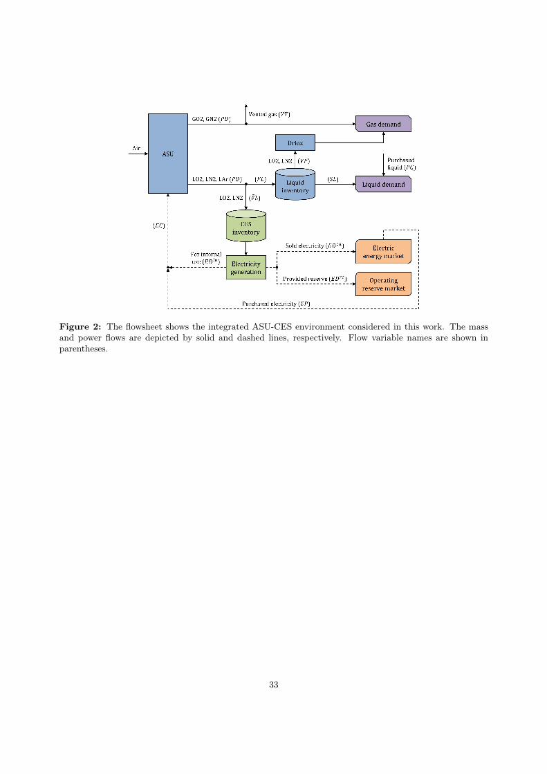
Figure 2: The flowsheet shows the integrated ASU-CES environment considered in this work. The massand power flows are depicted by solid and dashed lines, respectively. Flow variable names are shown inparentheses.

33

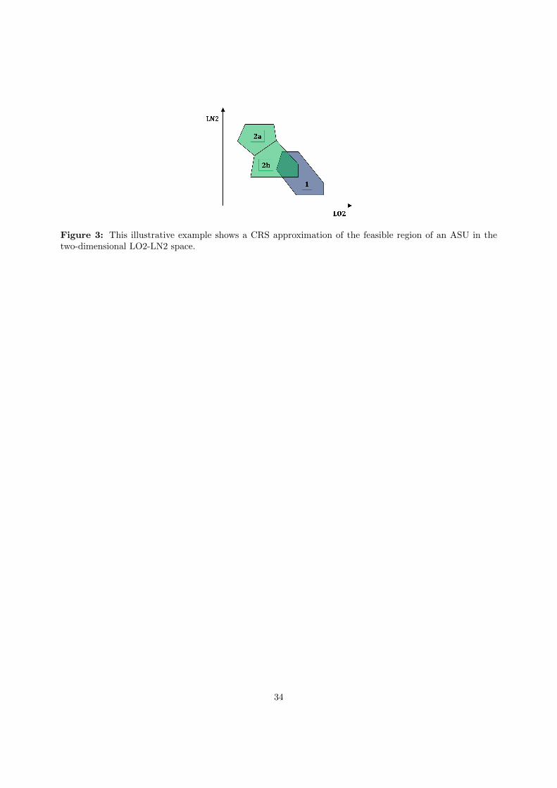
Figure 3: This illustrative example shows a CRS approximation of the feasible region of an ASU in thetwo-dimensional LO2-LN2 space.

34

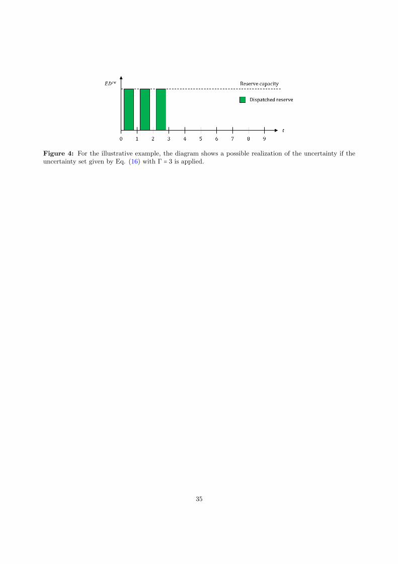
Figure 4: For the illustrative example, the diagram shows a possible realization of the uncertainty if theuncertainty set given by Eq. (16) with Γ = 3 is applied.

35

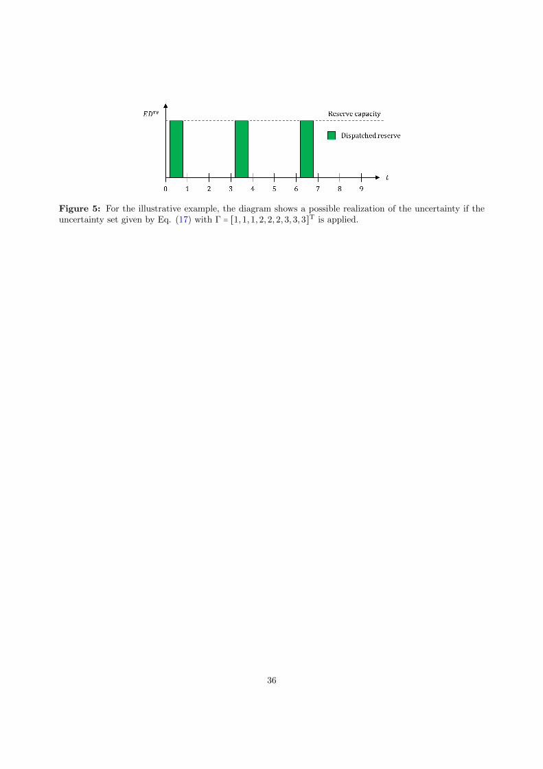
Figure 5: For the illustrative example, the diagram shows a possible realization of the uncertainty if theuncertainty set given by Eq. (17) with Γ = [1,1,1,2,2,2,3,3,3]T is applied.

36

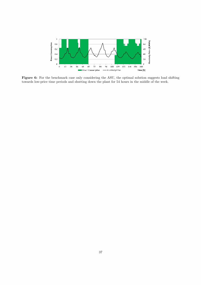
Figure 6: For the benchmark case only considering the ASU, the optimal solution suggests load shiftingtowards low-price time periods and shutting down the plant for 54 hours in the middle of the week.

37

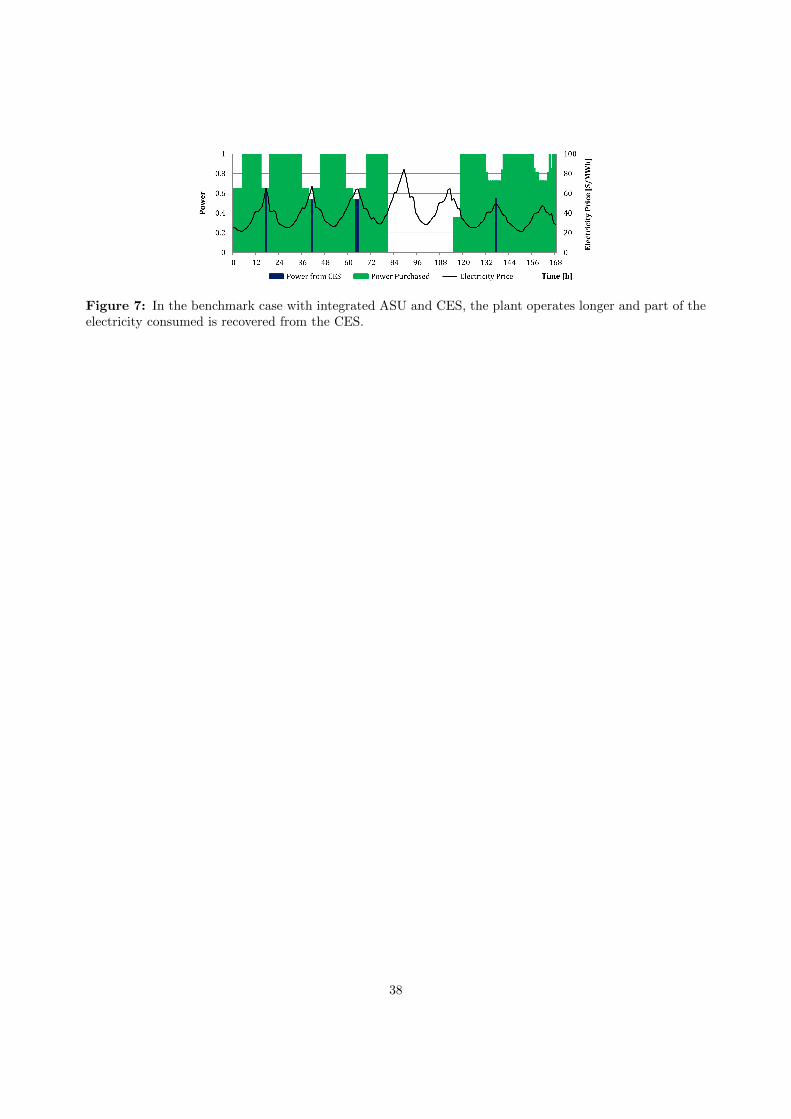
Figure 7: In the benchmark case with integrated ASU and CES, the plant operates longer and part of theelectricity consumed is recovered from the CES.

38

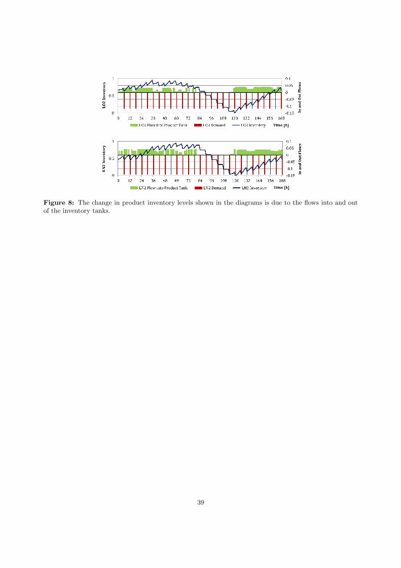
Figure 8: The change in product inventory levels shown in the diagrams is due to the flows into and outof the inventory tanks.

39

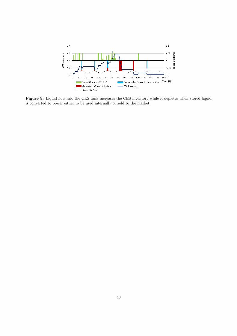
Figure 9: Liquid flow into the CES tank increases the CES inventory while it depletes when stored liquidis converted to power either to be used internally or sold to the market.

40

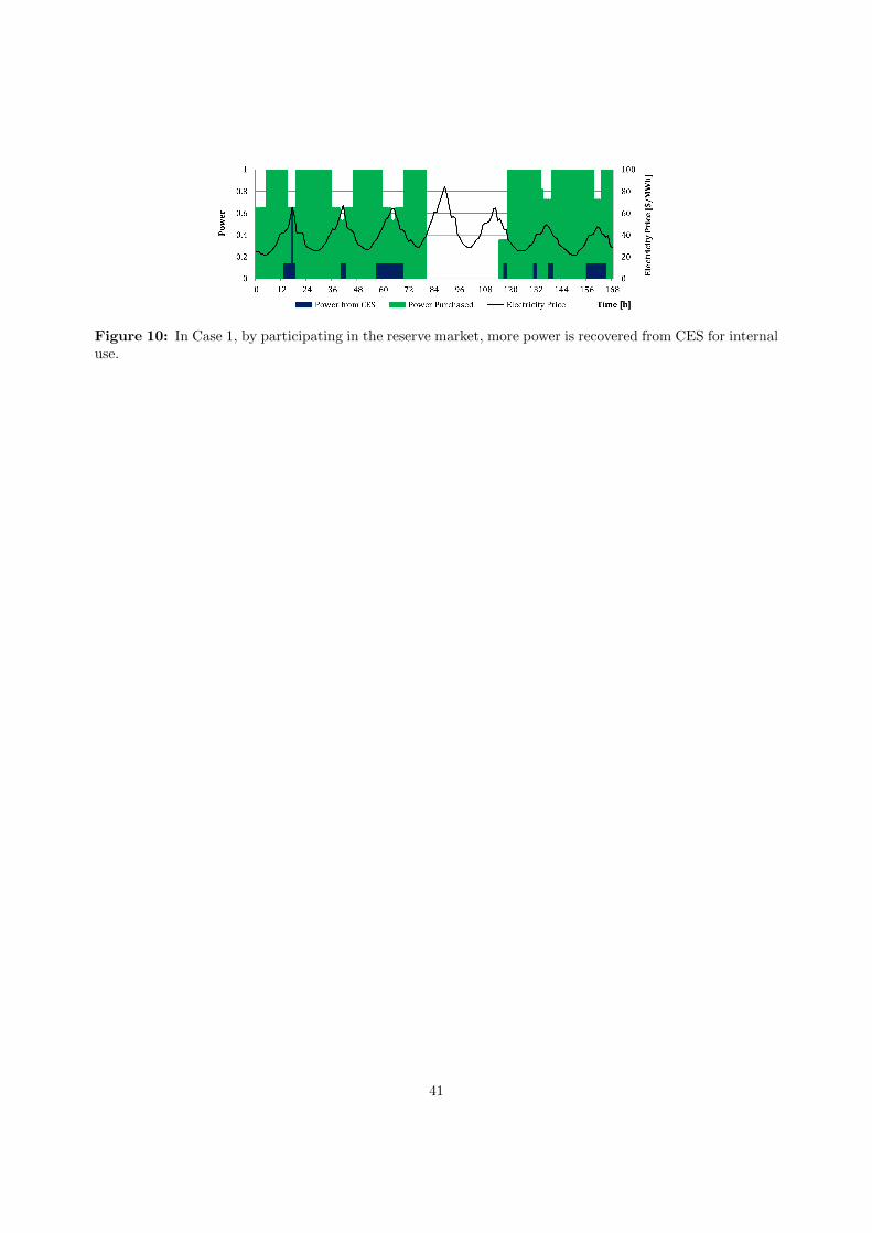
Figure 10: In Case 1, by participating in the reserve market, more power is recovered from CES for internaluse.

41

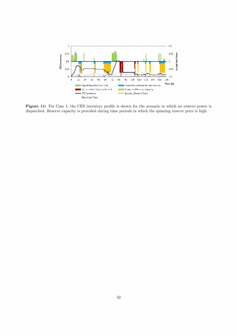
Figure 11: For Case 1, the CES inventory profile is shown for the scenario in which no reserve power isdispatched. Reserve capacity is provided during time periods in which the spinning reserve price is high.

42

Figure 12: The plot shows the CES inventory levels for Case 2 (top diagram) and Case 3 (bottom diagram).

43

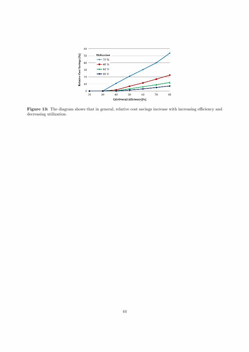
Figure 13: The diagram shows that in general, relative cost savings increase with increasing efficiency anddecreasing utilization.

44

List of Figure Captions

� Figure 1: The proposed model applies a common-grid time representation with a time period length

of ∆t and the present time point defined as time point 0.

� Figure 2: The flowsheet shows the integrated ASU-CES environment considered in this work. The

mass and power flows are depicted by solid and dashed lines, respectively. Flow variable names are

shown in parentheses.

� Figure 3: This illustrative example shows a CRS approximation of the feasible region of an ASU in

the two-dimensional LO2-LN2 space.

� Figure 4: For the illustrative example, the diagram shows a possible realization of the uncertainty if

the uncertainty set given by Eq. (16) with Γ = 3 is applied.

� Figure 5: For the illustrative example, the diagram shows a possible realization of the uncertainty if

the uncertainty set given by Eq. (17) with Γ = [1,1,1,2,2,2,3,3,3]T is applied.

� Figure 6: For the benchmark case only considering the ASU, the optimal solution suggests load

shifting towards low-price time periods and shutting down the plant for 54 hours in the middle of the

week.

� Figure 7: In the benchmark case with integrated ASU and CES, the plant operates longer and part

of the electricity consumed is recovered from the CES.

� Figure 8: The change in product inventory levels shown in the diagrams is due to the flows into and

out of the inventory tanks.

� Figure 9: Liquid flow into the CES tank increases the CES inventory while it depletes when stored

liquid is converted to power either to be used internally or sold to the market.

� Figure 10: In Case 1, by participating in the reserve market, more power is recovered from CES for

internal use.

45

� Figure 11: For Case 1, the CES inventory profile is shown for the scenario in which no reserve power

is dispatched. Reserve capacity is provided during time periods in which the spinning reserve price is

high.

� Figure 12: The plot shows the CES inventory levels for Case 2 (top diagram) and Case 3 (bottom

diagram).

� Figure 13: The diagram shows that in general, relative cost savings increase with increasing efficiency

and decreasing utilization.

46