Embed Size (px)
Citation preview
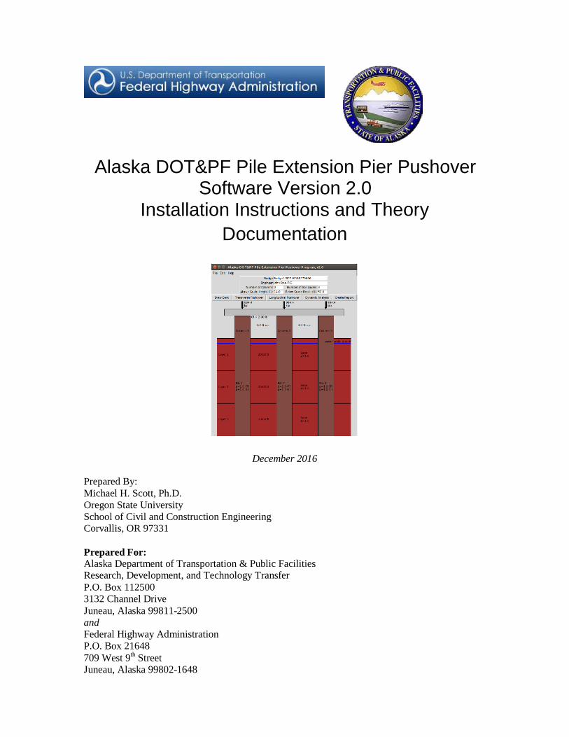
Alaska DOT&PF Pile Extension Pier Pushover Software Version 2.0
Installation Instructions and Documentation
Theory
December 2016
Prepared By: Michael H. Scott, Ph.D. Oregon State University School of Civil and Construction Engineering Corvallis, OR 97331
Prepared For: Alaska Department of Transportation & Public Facilities Research, Development, and Technology Transfer P.O. Box 112500 3132 Channel Drive Juneau, Alaska 99811-2500 and Federal Highway Administration P.O. Box 21648 709 West 9th Street Juneau, Alaska 99802-1648

IRIS # Z762870000
NSN 7540-01-280-5500 STANDARD FORM 298 (Rev. 2-98) Prescribed by ANSI Std. 239-18 298-102
REPORT DOCUMENTATION PAGE
Form approved OMB No.
Public reporting for this collection of information is estimated to average 1 hour per response, including the time for reviewing instructions, searching existing data sources, gathering and maintaining the data needed, and completing and reviewing the collection of information. Send comments regarding this burden estimate or any other aspect of this collection of information, including suggestion for reducing this burden to Washington Headquarters Services, Directorate for Information Operations and Reports, 1215 Jefferson Davis Highway, Suite 1204, Arlington, VA 22202-4302, and to the Office of Management and Budget, Paperwork Reduction Project (0704-1833), Washington, DC 20503 1. AGENCY USE ONLY (LEAVE BLANK)
4000(152)
2. REPORT DATE
December 31, 2016
3. REPORT TYPE AND DATES COVERED
FINAL, August 2015 – December 2016
4. TITLE AND SUBTITLE Alaska DOT&PF Pile Extension Pier Pushover Software Version 2.0 Installation Instructions and Theory Documentation
5. FUNDING NUMBERS
Federal # 4000(152)
6. AUTHOR(S) Michael H. Scott, Ph.D.
7. PERFORMING ORGANIZATION NAME(S) AND ADDRESS(ES) Oregon State University School of Civil and Construction Engineering Corvallis, OR 97331
8. PERFORMING ORGANIZATION REPORT NUMBER
4000(152)
9. SPONSORING/MONITORING AGENCY NAME(S) AND ADDRESS(ES)
Alaska Department of Transportation and Public Facilities Research, Development &Technology Transfer 3132 Channel Drive Juneau, Alaska 99811-2500
10. SPONSORING/MONITORING AGENCY REPORT NUMBER
4000(152)
11. SUPPLEMENTARY NOTES
12a. DISTRIBUTION / AVAILABILITY STATEMENT
Copies available online at http://www.dot.alaska.gov/stwddes/research/search_lib.shtml
12b. DISTRIBUTION CODE
13. ABSTRACT (Maximum 200 words)
The updated pushover software accommodates conventional reinforced concrete columns and drilled shafts and allows for changes in cross-sections so that other systems (e.g., enlarged drilled shaft supporting smaller diameter concrete column) can be modeled. Additional soil spring modifies have been added as well as cap beam forces, zero deflection points and longitudinal analysis options.
14. KEYWORDS : pushover software, pile design, seismic, bridge design, transverse pushover
15. NUMBER OF PAGES 52
16. PRICE CODE N/A
17. SECURITY CLASSIFICATION OF REPORT Unclassified
18. SECURITY CLASSIFICATION OF THIS PAGE Unclassified
19. SECURITY CLASSIFICATION OF ABSTRACT Unclassified
20. LIMITATION OF ABSTRACT
None

Notice This document is disseminated under the sponsorship of the U.S. Department of Transportation in the interest of information exchange. The U.S. Government assumes no liability for the use of the information contained in this document.
The U.S. Government does not endorse products or manufacturers. Trademarks or manufacturers’ names appear in this report only because they are considered essential to the objective of the document.
Quality Assurance Statement
The Federal Highway Administration (FHWA) provides high-quality information to serve Government, industry, and the public in a manner that promotes public understanding. Standards and policies are used to ensure and maximize the quality, objectivity, utility, and integrity of its information. FHWA periodically reviews quality issues and adjusts its programs and processes to ensure continuous quality improvement.
Author’s Disclaimer
Opinions and conclusions expressed or implied in the report are those of the author. They are not necessarily those of the Alaska DOT&PF or funding agencies.
in2 mm2
square inches 645.2 square millimeters
oF oC Fahrenheit 5 (F-32)/9 Celsius
candela/m2 cd/m2
fl foot-Lamberts 3.426
mm2
m2
in2
yd2
square millimeters 0.0016 square inches
square meters 1.195 square yards
oC oF Celsius 1.8C+32 Fahrenheit
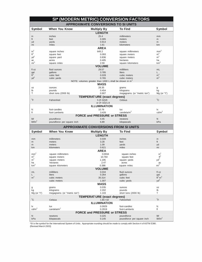
*SI is the symbol for the International System of Units. Appropriate rounding should be made to comply with Section 4 of ASTM E380. (Revised March 2003)
SI* (MODERN METRIC) CONVERSION FACTORS APPROXIMATE CONV ERSIONS TO SI UNITS
Symbol When You Know Multiply By To Find Symbol LENGTH
in inches 25.4 millimeters mm ft feet 0.305 meters m yd yards 0.914 meters m mi miles 1.61 kilometers km
AREA
ft2 square feet 0.093 square meters m2
yd2 square yard 0.836 square meters m2
ac acres 0.405 hectares ha mi2 square miles 2.59 square kilometers km2
VOLUME fl oz fluid ounces 29.57 milliliters mL gal gallons 3.785 liters L ft3 cubic feet 0.028 cubic meters m3
yd3 cubic yards 0.765 cubic meters m3
NOTE: volumes greater than 1000 L shall be shown in m3
MASS oz ounces 28.35 grams g lb pounds 0.454 kilograms kg T short tons (2000 lb) 0.907 megagrams (or "metric ton") Mg (or "t")
TEMPERAT URE (exact degrees)
or (F-32)/1.8 ILLUMINATI ON
fc foot-candles 10.76 lux lx
FORCE and PRESSURE or STRESS lbf poundforce 4.45 newtons N lbf/in2 poundforce per square inch 6.89 kilopascals kPa
APPROXIMATE CONV ERSIONS FROM SI UNITS Symbol When You Know Multiply By To Find Symbol
LENGTH mm millimeters 0.039 inches in m meters 3.28 feet ft m meters 1.09 yards yd km kilometers 0.621 miles mi
AREA
m2 square meters 10.764 square feet ft2
ha hectares 2.47 acres ac km2 square kilometers 0.386 square miles mi2
VOLUME mL milliliters 0.034 fluid ounces fl oz L liters 0.264 gallons gal m3 cubic meters 35.314 cubic feet ft3 m3
cubic meters 1.307 cubic yards yd3
MASS g grams 0.035 ounces oz kg kilograms 2.202 pounds lb Mg (or "t") megagrams (or "metric ton") 1.103 short tons (2000 lb) T
TEMPERAT URE (exact degrees)
ILLUMINATI ON lx lux 0.0929 foot-candles fc cd/m2 candela/m2 0.2919 foot-Lamberts fl
FORCE and PRESSURE or STRESS N newtons 0.225 poundforce lbf kPa kilopascals 0.145 poundforce per square inch lbf/in2

Alaska DOT&PF Pile Extension Pier Pushover Software Version 2.0
Installation Instructions and Theory Documentation
December 2016
Prepared for: Alaska Department of Transportation and Public Facilities
3132 Channel Drive Juneau, AK 99811
Prepared by: Michael H. Scott
Oregon State University School of Civil and Construction Engineering
Corvallis, OR 97331
1
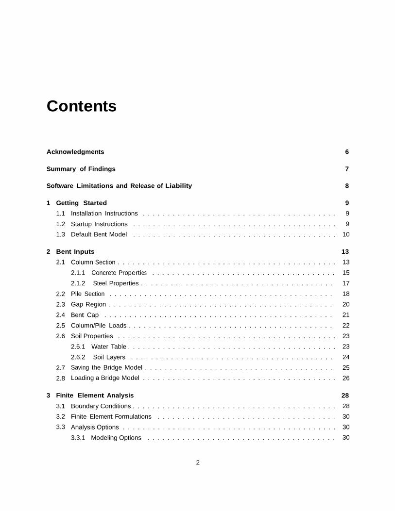
Contents
Acknowledgments 6
Summary of Findings 7
Software Limitations and Release of Liability 8
1 Getting Started 9 9 9
10
1.1 1.2 1.3
Installation Instructions . . . . . . . . . . . . . . . . . . . . . . . . . . . . . . . . . . . . . . . Startup Instructions Default Bent Model
. . . . . . . . . . . . . . . . . . . . . . . . . . . . . . . . . . . . . . . . .
. . . . . . . . . . . . . . . . . . . . . . . . . . . . . . . . . . . . . . . . .
2 Bent Inputs 13 13 15 17 18 20 21 22 23 23 24 25 26
2.1 Column Section . . . . . . . . . . . . . . . . . . . . . . . . . . . . . . . . . . . . . . . . . . . . 2.1.1 Concrete Properties . . . . . . . . . . . . . . . . . . . . . . . . . . . . . . . . . . . . . 2.1.2 Steel Properties . . . . . . . . . . . . . . . . . . . . . . . . . . . . . . . . . . . . . . . Pile Section . . . . . . . . . . . . . . . . . . . . . . . . . . . . . . . . . . . . . . . . . . . . . . Gap Region . . . . . . . . . . . . . . . . . . . . . . . . . . . . . . . . . . . . . . . . . . . . . . Bent Cap . . . . . . . . . . . . . . . . . . . . . . . . . . . . . . . . . . . . . . . . . . . . . . . Column/Pile Loads . . . . . . . . . . . . . . . . . . . . . . . . . . . . . . . . . . . . . . . . . . Soil Properties . . . . . . . . . . . . . . . . . . . . . . . . . . . . . . . . . . . . . . . . . . . . 2.6.1 Water Table . . . . . . . . . . . . . . . . . . . . . . . . . . . . . . . . . . . . . . . . . . 2.6.2 Soil Layers . . . . . . . . . . . . . . . . . . . . . . . . . . . . . . . . . . . . . . . . . Saving the Bridge Model . . . . . . . . . . . . . . . . . . . . . . . . . . . . . . . . . . . . . . Loading a Bridge Model . . . . . . . . . . . . . . . . . . . . . . . . . . . . . . . . . . . . . . .
2.2 2.3 2.4 2.5 2.6
2.7 2.8
3 Finite Element Analysis 28 28 30 30 30
3.1 3.2 3.3
Boundary Conditions . . . . . . . . . . . . . . . . . . . . . . . . . . . . . . . . . . . . . . . . . Finite Element Formulations . . . . . . . . . . . . . . . . . . . . . . . . . . . . . . . . . . . . Analysis Options . . . . . . . . . . . . . . . . . . . . . . . . . . . . . . . . . . . . . . . . . . . 3.3.1 Modeling Options . . . . . . . . . . . . . . . . . . . . . . . . . . . . . . . . . . . . . .
2
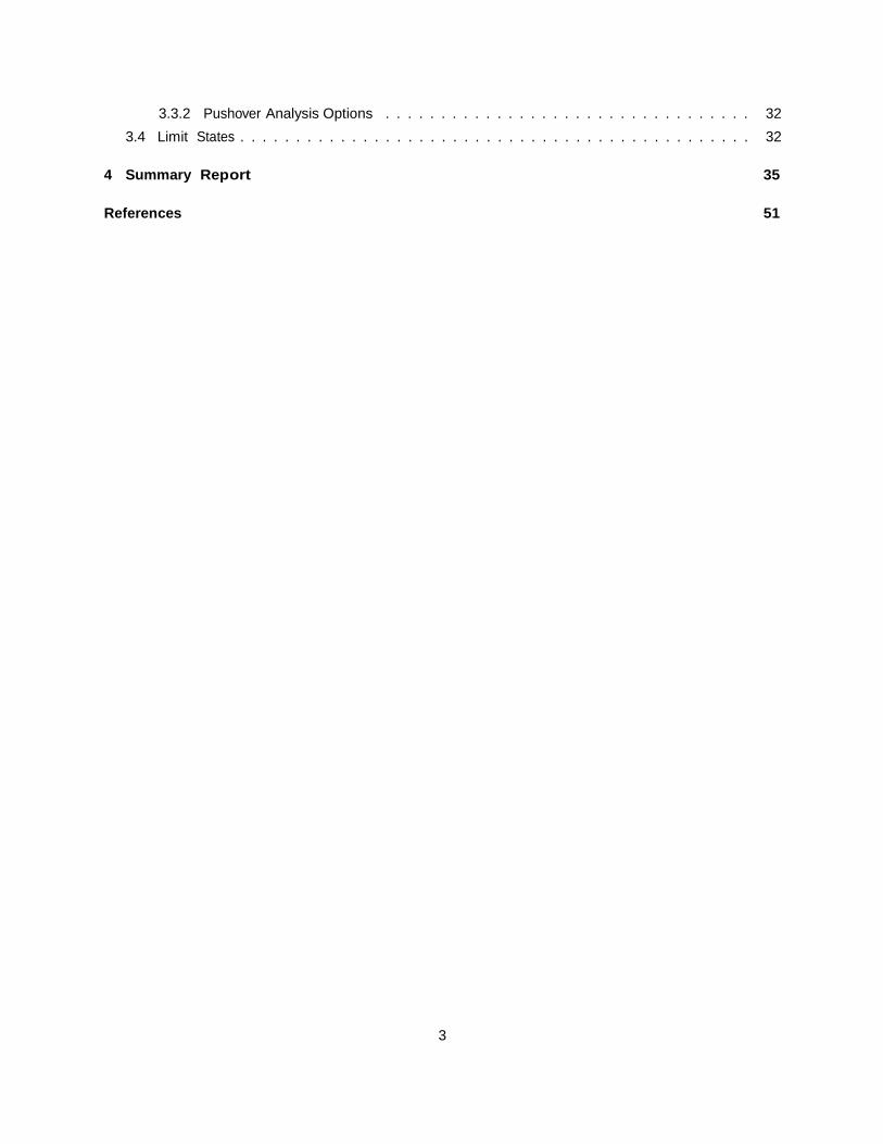
3.3.2 Pushover Analysis Options . . . . . . . . . . . . . . . . . . . . . . . . . . . . . . . . . 3.4 Limit States . . . . . . . . . . . . . . . . . . . . . . . . . . . . . . . . . . . . . . . . . . . . . .
32 32
4 Summary Report 35
References 51
3
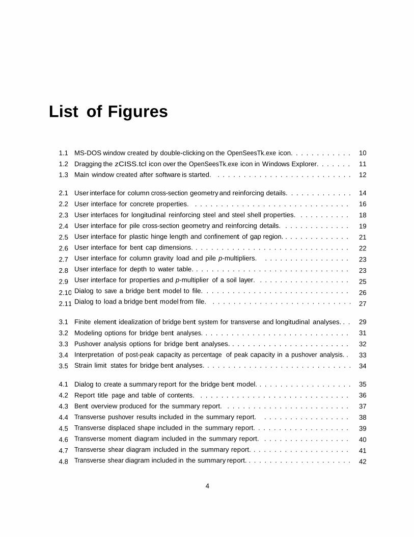
List of Figures
1.1 1.2 1.3
MS-DOS window created by double-clicking on the OpenSeesTk.exe icon. . . . . . . . . . . . Dragging the zCISS.tcl icon over the OpenSeesTk.exe icon in Windows Explorer. . . . . . . Main window created after software is started. . . . . . . . . . . . . . . . . . . . . . . . . . .
10 11 12
2.1 2.2 2.3 2.4 2.5 2.6 2.7 2.8 2.9 2.10 2.11
User interface for column cross-section geometry and reinforcing details. . . . . . . . . . . . . User interface for concrete properties. . . . . . . . . . . . . . . . . . . . . . . . . . . . . . . . User interfaces for longitudinal reinforcing steel and steel shell properties. . . . . . . . . . . . User interface for pile cross-section geometry and reinforcing details. . . . . . . . . . . . . . . User interface for plastic hinge length and confinement of gap region. . . . . . . . . . . . . . . User interface for bent cap dimensions. . . . . . . . . . . . . . . . . . . . . . . . . . . . . . . . User interface for column gravity load and pile p-multipliers. . . . . . . . . . . . . . . . . . . User interface for depth to water table. . . . . . . . . . . . . . . . . . . . . . . . . . . . . . . . User interface for properties and p-multiplier of a soil layer. . . . . . . . . . . . . . . . . . . . Dialog to save a bridge bent model to file. . . . . . . . . . . . . . . . . . . . . . . . . . . . . . Dialog to load a bridge bent model from file. . . . . . . . . . . . . . . . . . . . . . . . . . . .
14 16 18 19 21 22 23 23 25 26 27
3.1 3.2 3.3 3.4 3.5
Finite element idealization of bridge bent system for transverse and longitudinal analyses. . . Modeling options for bridge bent analyses. . . . . . . . . . . . . . . . . . . . . . . . . . . . . Pushover analysis options for bridge bent analyses. . . . . . . . . . . . . . . . . . . . . . . . Interpretation of post-peak capacity as percentage of peak capacity in a pushover analysis. . Strain limit states for bridge bent analyses. . . . . . . . . . . . . . . . . . . . . . . . . . . . .
29 31 32 33 34
4.1 4.2 4.3 4.4 4.5 4.6 4.7 4.8
Dialog to create a summary report for the bridge bent model. . . . . . . . . . . . . . . . . . . Report title page and table of contents. . . . . . . . . . . . . . . . . . . . . . . . . . . . . . Bent overview produced for the summary report. . . . . . . . . . . . . . . . . . . . . . . . . Transverse pushover results included in the summary report. . . . . . . . . . . . . . . . . . Transverse displaced shape included in the summary report. . . . . . . . . . . . . . . . . . . Transverse moment diagram included in the summary report. . . . . . . . . . . . . . . . . . Transverse shear diagram included in the summary report. . . . . . . . . . . . . . . . . . . . Transverse shear diagram included in the summary report. . . . . . . . . . . . . . . . . . . . .
35 36 37 38 39 40 41 42
4
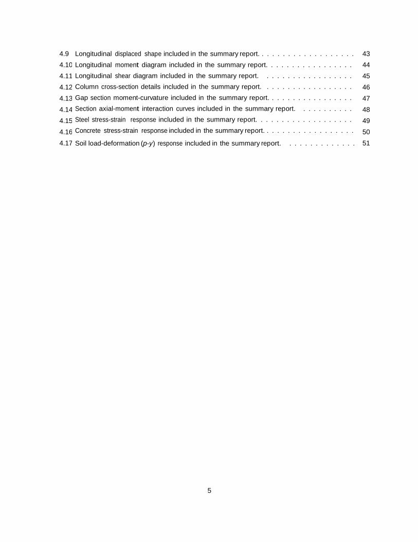
4.9 4.10 4.11 4.12 4.13 4.14 4.15 4.16 4.17
Longitudinal displaced shape included in the summary report. . . . . . . . . . . . . . . . . . . Longitudinal moment diagram included in the summary report. . . . . . . . . . . . . . . . . Longitudinal shear diagram included in the summary report. . . . . . . . . . . . . . . . . . Column cross-section details included in the summary report. . . . . . . . . . . . . . . . . . Gap section moment-curvature included in the summary report. . . . . . . . . . . . . . . . . Section axial-moment interaction curves included in the summary report. . . . . . . . . . . . Steel stress-strain response included in the summary report. . . . . . . . . . . . . . . . . . . Concrete stress-strain response included in the summary report. . . . . . . . . . . . . . . . . .
43 44 45 46 47 48 49 50 51 Soil load-deformation (p-y) response included in the summary report. . . . . . . . . . . . . .
5

Acknowledgments
This work has been supported by the Alaska Department of Transportation and Public Facilities (AK- DOT&PF). Any opinions expressed in this work are those of the author and do not necessarily reflect the views of the funding agency.
6
Summary of Findings
The software described herein is built around free components, namely Tcl/Tk, a string-based scripting lan- guage with widgets for developing graphical user interfaces (GUIs), and OpenSees, an open source nonlinear finite element analysis software framework. This combination of Tcl/Tk and OpenSees allowed for rapid prototyping of GUIs that interact with state-of-the-art element and constitutive models for the analysis of cast-in-steel shell (CISS) bents. From a computational point-of-view, very little “from-scratch” coding was required as modules available in OpenSees were repackaged to meet AKDOT&PF’s needs. This development approach will be fruitful for future AKDOT&PF software projects and potentially for commercialization and technology transfer. Based on collaboration and feedback from Mr. Elmer Marx, the software was found to be generally easy to use for analyzing a wide range of CISS bents in the AKDOT&PF inventory and more efficient compared to the variety of separate software previously used for such analyses.
7
Software Limitations and Release of
Liability
The Alaska DOT&PF Pile Extension Pier Pushover Software is a powerful tool that includes geometric and material nonlinearities, both structural material and soil, in determining the lateral load-deflection response of bridge piers. The results of any analysis are sensitive to the input parameters. The engineer must be fully aware of the assumptions and limitations described in this document, as well as those that are part of the greater body of engineering knowledge, when using the software. As with all engineering software, the results should be verified by a professionally licensed engineer.
The user agrees to indemnify and hold the States of Alaska and Oregon harmless from any claim or demand, including attorneys’ fees, made by any third party as a result of using the software.
8
Chapter 1
Getting Started
The zCISS software is developed using the Tcl/Tk scripting language for model generation and graphical user interfaces in conjunction with OpenSees as its computational engine for nonlinear finite element analysis. The combined use of OpenSees and Tcl/Tk makes zCISS platform-independent, with only aesthetic differences in the GUI. The installation and startup instructions described in this chapter are based on the Windows operating system.
1.1 Installation Instructions
The user is required to install Tcl/Tk (64-bit) version 8.6 or later, which is available free of charge at
http://www.activestate.com/activetcl
In addition, the user must have the Tk-version (64-bit) of OpenSees (OpenSeesTk.exe) installed, which can also be downloaded for free at
http://opensees.berkeley.edu
1.2 Startup Instructions
With OpenSeesTk.exe and zCISS.tcl installed in the same directory, there are two options to start the software under the Windows operating system.
1. Double-click on the OpenSeesTk.exe icon. An MS-DOS window will then appear showing OpenSees copyright information along with an interactive prompt. In addition, there will be a plain grey window titled openSeesTk, as shown in Figure 1.1. At the prompt in the MS-DOS window, type source zCISS.tcl (also shown in the figure). This will cause the plain grey window to change to the zCISS startup window shown in Figure 1.3.
9
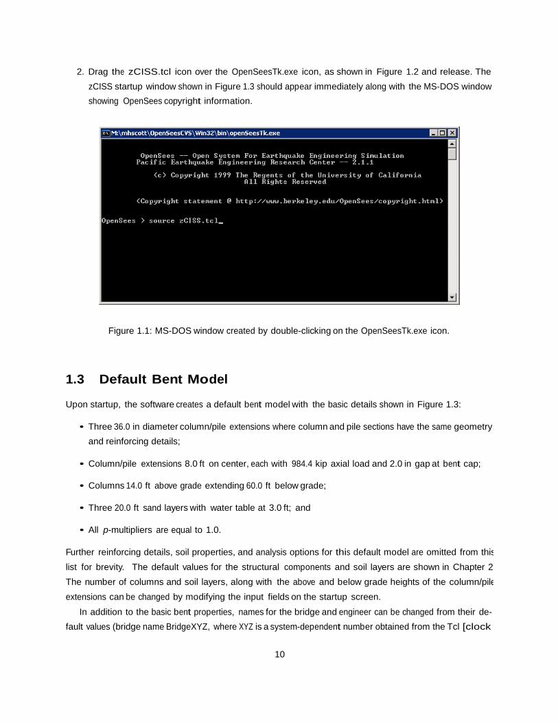
2. Drag the zCISS.tcl icon over the OpenSeesTk.exe icon, as shown in Figure 1.2 and release. The zCISS startup window shown in Figure 1.3 should appear immediately along with the MS-DOS window showing OpenSees copyright information.
Figure 1.1: MS-DOS window created by double-clicking on the OpenSeesTk.exe icon.
1.3 Default Bent Model
Upon startup, the software creates a default bent model with the basic details shown in Figure 1.3:
• Three 36.0 in diameter column/pile extensions where column and pile sections have the same geometry and reinforcing details;
• Column/pile extensions 8.0 ft on center, each with 984.4 kip axial load and 2.0 in gap at bent cap;
• Columns 14.0 ft above grade extending 60.0 ft below grade;
• Three 20.0 ft sand layers with water table at 3.0 ft; and
• All p-multipliers are equal to 1.0. Further reinforcing details, soil properties, and analysis options for this default model are omitted from this list for brevity. The default values for the structural components and soil layers are shown in Chapter 2. The number of columns and soil layers, along with the above and below grade heights of the column/pile extensions can be changed by modifying the input fields on the startup screen.
In addition to the basic bent properties, names for the bridge and engineer can be changed from their de- fault values (bridge name BridgeXYZ, where XYZ is a system-dependent number obtained from the Tcl [clock
10
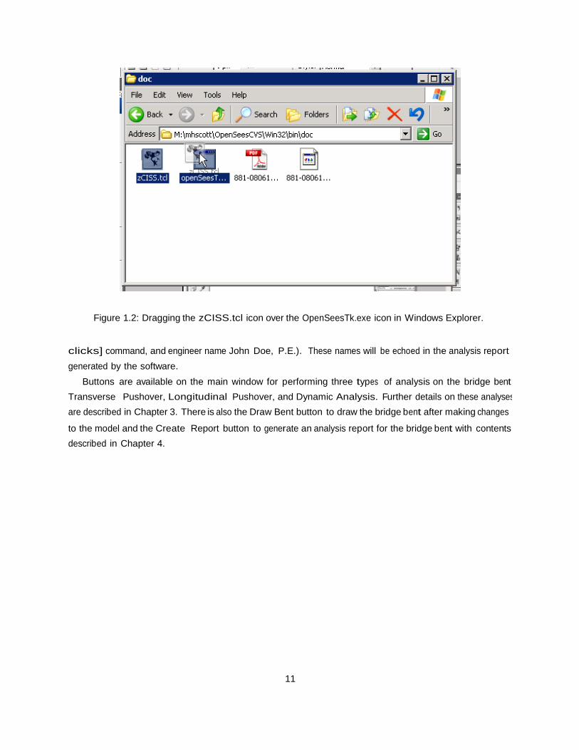
Figure 1.2: Dragging the zCISS.tcl icon over the OpenSeesTk.exe icon in Windows Explorer.
clicks] command, and engineer name John Doe, P.E.). These names will be echoed in the analysis report generated by the software.
Buttons are available on the main window for performing three types of analysis on the bridge bent: Transverse Pushover, Longitudinal Pushover, and Dynamic Analysis. Further details on these analyses are described in Chapter 3. There is also the Draw Bent button to draw the bridge bent after making changes
to the model and the Create described in Chapter 4.
Report button to generate an analysis report for the bridge bent with contents
11
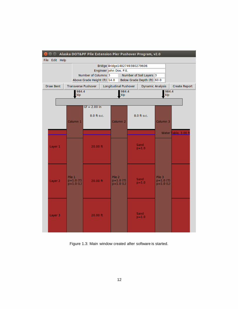
Figure 1.3: Main window created after software is started.
12
Chapter 2
Bent Inputs
Inputs for the column/pile extensions, bentcap, and soil are described in this chapter along with details on saving the bent model to a file and loading previously saved models.
2.1 Column Section
The geometry and reinforcing details are assumed to be the same for each column in the bridge bent. Use one of the following two methods to view and edit the column cross-section:
• Double-click on a column in the main window (Figure 1.3); or
• Select Edit -> Section -> Column from the main menu.
After using one of these methods to access the column cross-section, the user interface shown in Figure 2.1 appears. Properties for the Steel Shell, Longitudinal Reinforcement, and Transverse Reinforcement can be modified through this interface.
Steel Shell
• Diameter – outer diameter of the steel shell
Units: in, Default: 36.0 in
• Thickness – thickness of the steel shell
Units: in, Default: 0.75 in
Note: set this value to zero in order to remove the steel shell
Longitudinal Reinforcement
• Clear Cover – distance from outer face of spiral transverse reinforcement to inside of steel shell
Units: in, Default: 2.0
13
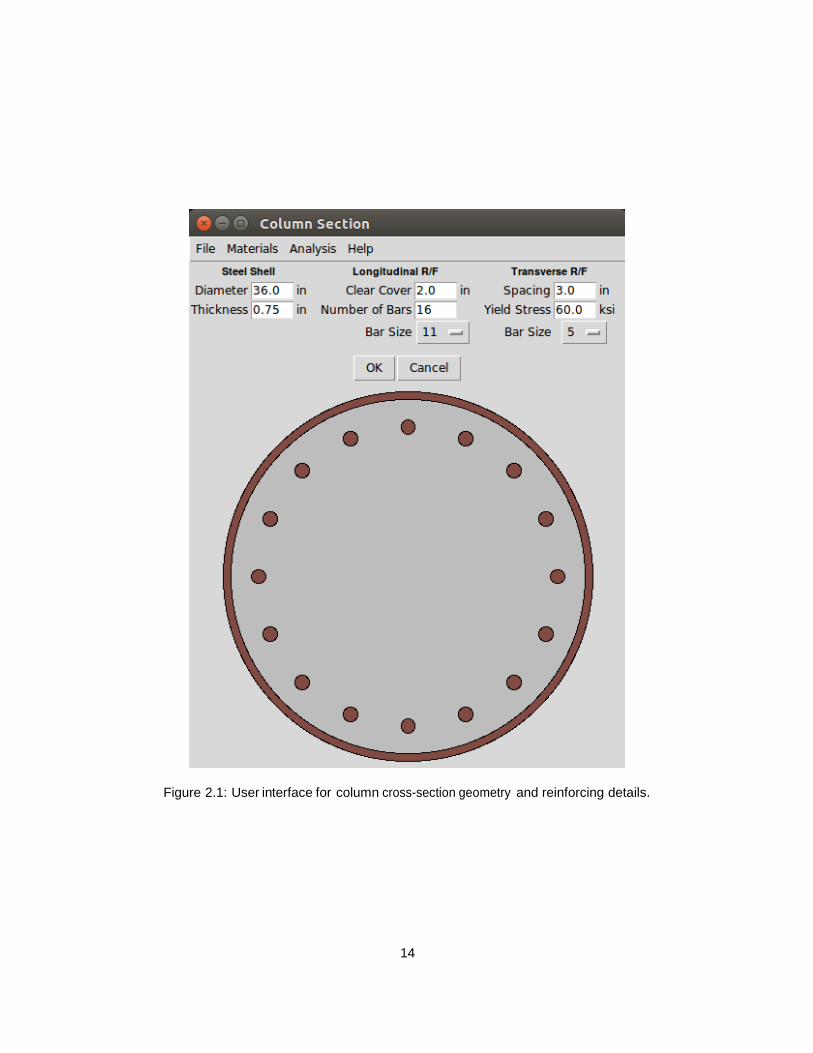
Figure 2.1: User interface for column cross-section geometry and reinforcing details.
14
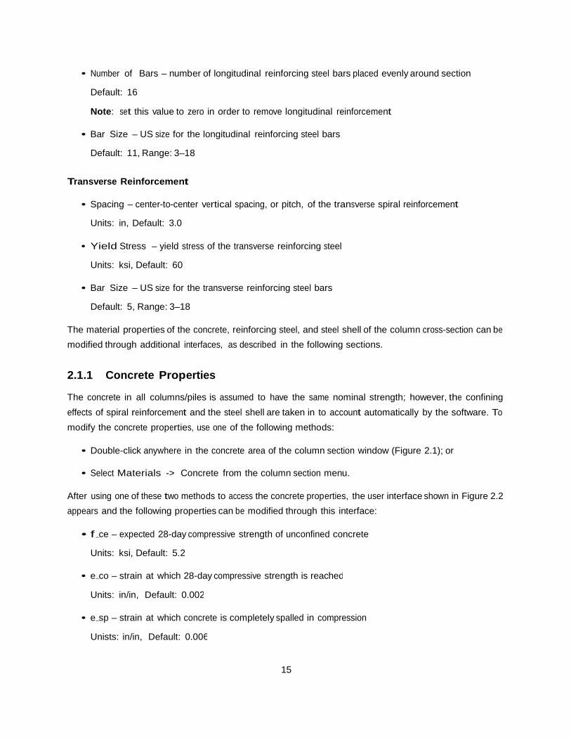
• Number of Bars – number of longitudinal reinforcing steel bars placed evenly around section
Default: 16
Note: set this value to zero in order to remove longitudinal reinforcement
• Bar Size – US size for the longitudinal reinforcing steel bars
Default: 11, Range: 3–18
Transverse Reinforcement
• Spacing – center-to-center vertical spacing, or pitch, of the transverse spiral reinforcement
Units: in, Default: 3.0
• Yield Stress – yield stress of the transverse reinforcing steel
Units: ksi, Default: 60
• Bar Size – US size for the transverse reinforcing steel bars
Default: 5, Range: 3–18
The material properties of the concrete, reinforcing steel, and steel shell of the column cross-section can be modified through additional interfaces, as described in the following sections.
2.1.1 Concrete Properties
The concrete in all columns/piles is assumed to have the same nominal strength; however, the confining effects of spiral reinforcement and the steel shell are taken in to account automatically by the software. To modify the concrete properties, use one of the following methods:
• Double-click anywhere in the concrete area of the column section window (Figure 2.1); or
• Select Materials -> Concrete from the column section menu.
After using one of these two methods to access the concrete properties, the user interface shown in Figure 2.2 appears and the following properties can be modified through this interface:
• f ce – expected 28-day compressive strength of unconfined concrete
Units: ksi, Default: 5.2
• e co – strain at which 28-day compressive strength is reached
Units: in/in, Default: 0.002
• e sp – strain at which concrete is completely spalled in compression
Unists: in/in, Default: 0.006
15
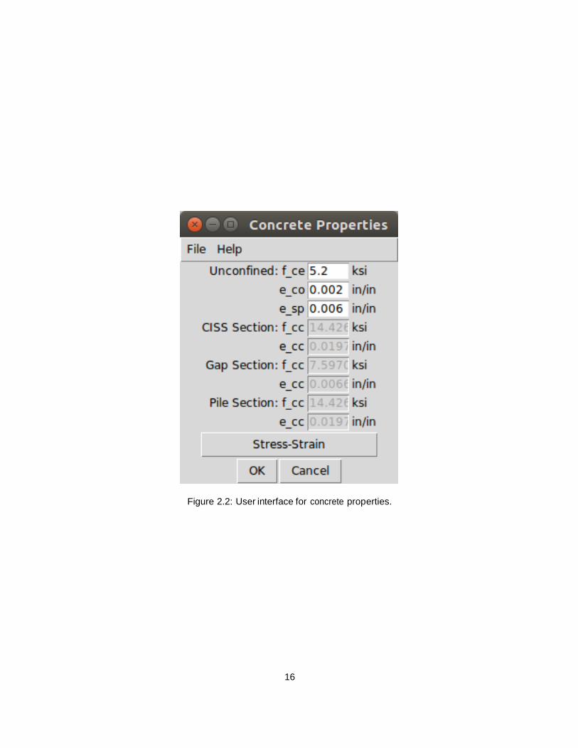
Figure 2.2: User interface for concrete properties.
16
Using the unconfined concrete properties, the software computes automatically the compressive strength, fcc, and corresponding strain, ecc, for the gap section, steel shell column section, and steel shell pile section. Concrete confinement in the gap section is based on the model proposed by Mander [4] while confinement for the column and pile sections wrapped in a steel shell is based on the model proposed by Chai et al [1]. The confined concrete properties based on these models is shown in Figure 2.2 for the default values of unconfined concrete strength. The unconfined concrete behavior is based on the model proposed by Kent et al [3]. There is also a button, Stress-Strain, to generate and view the stress-strain curves for each concrete model. This information is also echoed in the report generated by the software, as described in Chapter 4, and will not be described here.
2.1.2 Steel Properties
Similar to the concrete, the steel properties are assumed to be the same in all columns/piles of the bridge bent model; however, the longitudinal reinforcing steel and steel shell may have different properties. To modify the reinforcing steel properties, use one of the following methods:
• Double-click on one of the reinforcing bars in the column section window (Figure 2.1); or
• Select Materials -> Reinforcing Steel from the column section menu.
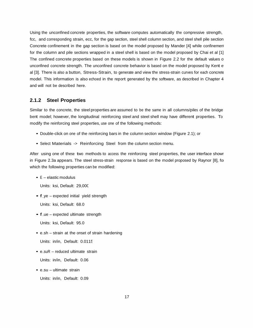
After using one of these two methods to access the reinforcing steel properties, the user interface shown in Figure 2.3a appears. The steel stress-strain response is based on the model proposed by Raynor [8], for which the following properties can be modified:
• E – elastic modulus
Units: ksi, Default: 29,000
• f ye – expected initial yield strength
Units: ksi, Default: 68.0
• f ue – expected ultimate strength
Units: ksi, Default: 95.0
• e sh – strain at the onset of strain hardening
Units: in/in, Default: 0.0115
• e suR – reduced ultimate strain
Units: in/in, Default: 0.06
• e su – ultimate strain
Units: in/in, Default: 0.09
17
• C1 – power curve parameter
Default: 1.5
(a) Reinforcing steel. (b) Steel shell.
Figure 2.3: User interfaces for longitudinal reinforcing steel and steel shell properties.
There is also a button, Stress-Strain, to generate and view the stress-strain curves for the reinforcing steel. This information is also echoed in the report generated by the software, as described in Chapter 4, and will not be described here. The stress-strain behavior of the steel shell follows the same Raynor model as that used for the reinforcing steel; however, the default values differ, as shown in Figure 2.3b. To modify the steel shell properties, use one of the following methods:
• Double-click on the steel shell in the column section window (Figure 2.1); or
• Select Materials -> Steel Shell from the column section menu. After using one of these two methods to access the reinforcing steel properties, the user interface shown in Figure 2.3b appears.
2.2 Pile Section
Like the columns, the geometry and reinforcing details are assumed to be the same for each pile in the bridge bent. Use one of the two following methods to view and edit the pile cross-section:
18
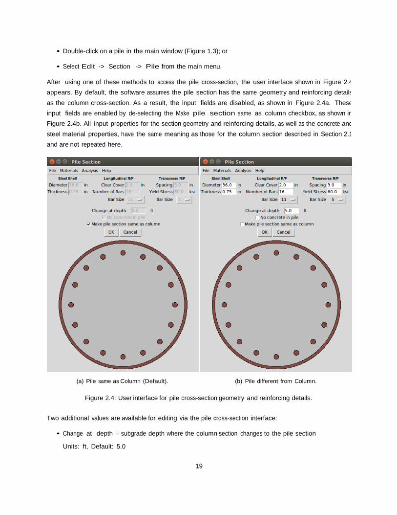
• Double-click on a pile in the main window (Figure 1.3); or
• Select Edit -> Section -> Pile from the main menu.
After using one of these methods to access the pile cross-section, the user interface shown in Figure 2.4 appears. By default, the software assumes the pile section has the same geometry and reinforcing details as the column cross-section. As a result, the input fields are disabled, as shown in Figure 2.4a. These input fields are enabled by de-selecting the Make pile section same as column checkbox, as shown in Figure 2.4b. All input properties for the section geometry and reinforcing details, as well as the concrete and steel material properties, have the same meaning as those for the column section described in Section 2.1 and are not repeated here.
(a) Pile same as Column (Default). (b) Pile different from Column.
Figure 2.4: User interface for pile cross-section geometry and reinforcing details.
Two additional values are available for editing via the pile cross-section interface:
• Change at depth – subgrade depth where the column section changes to the pile section
Units: ft, Default: 5.0
19
• No concrete in pile – option to remove concrete and reinforcing steel, making the pile section a hollow steel shell
Default: False
2.3 Gap Region
The length of the gap between the steel shell at the column to bent cap connection, along with the plastic hinge length and concrete confinement in the gap region can be accessed and edited using one of the following methods:
• Double-click on the Gf=XX in text in the main window (Figure 1.3); or
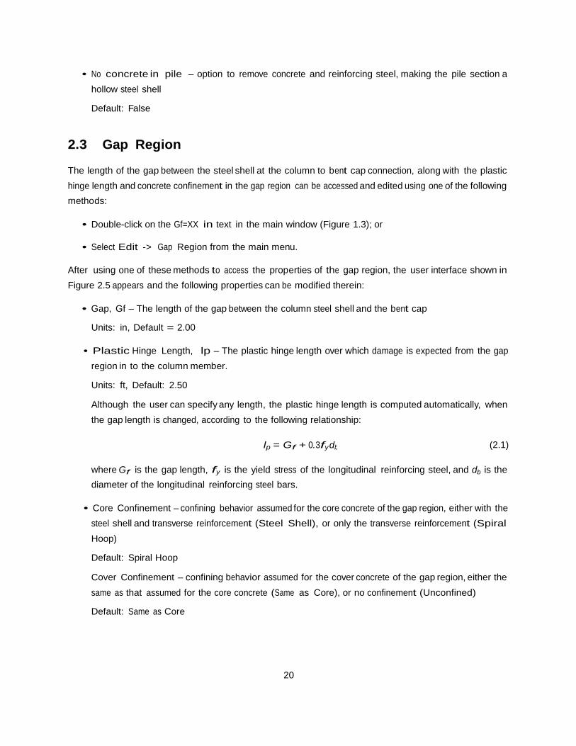
• Select Edit -> Gap Region from the main menu. After using one of these methods to access the properties of the gap region, the user interface shown in Figure 2.5 appears and the following properties can be modified therein:
• Gap, Gf – The length of the gap between the column steel shell and the bent cap
Units: in, Default = 2.00
• Plastic Hinge Length, lp – The plastic hinge length over which damage is expected from the gap region in to the column member.
Units: ft, Default: 2.50
Although the user can specify any length, the plastic hinge length is computed automatically, when the gap length is changed, according to the following relationship:
lp = Gf + 0.3fy db (2.1)
where Gf is the gap length, fy is the yield stress of the longitudinal reinforcing steel, and db is the diameter of the longitudinal reinforcing steel bars.
• Core Confinement – confining behavior assumed for the core concrete of the gap region, either with the steel shell and transverse reinforcement (Steel Shell), or only the transverse reinforcement (Spiral Hoop)
Default: Spiral Hoop
Cover Confinement – confining behavior assumed for the cover concrete of the gap region, either the same as that assumed for the core concrete (Same as Core), or no confinement (Unconfined) Default: Same as Core
20
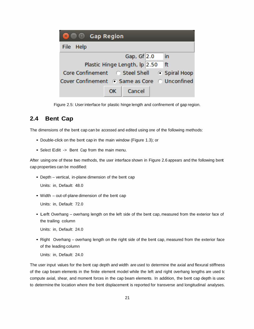
Figure 2.5: User interface for plastic hinge length and confinement of gap region.
2.4 Bent Cap
The dimensions of the bent cap can be accessed and edited using one of the following methods:
• Double-click on the bent cap in the main window (Figure 1.3); or
• Select Edit -> Bent Cap from the main menu.
After using one of these two methods, the user interface shown in Figure 2.6 appears and the following bent cap properties can be modified:
• Depth – vertical, in-plane dimension of the bent cap
Units: in, Default: 48.0
• Width – out-of-plane dimension of the bent cap
Units: in, Default: 72.0
• Left Overhang – overhang length on the left side of the bent cap, measured from the exterior face of the trailing column
Units: in, Default: 24.0
• Right Overhang – overhang length on the right side of the bent cap, measured from the exterior face of the leading column
Units: in, Default: 24.0
The user input values for the bent cap depth and width are used to determine the axial and flexural stiffness of the cap beam elements in the finite element model while the left and right overhang lengths are used to compute axial, shear, and moment forces in the cap beam elements. In addition, the bent cap depth is used to determine the location where the bent displacement is reported for transverse and longitudinal analyses.
21

Figure 2.6: User interface for bent cap dimensions.
2.5 Column/Pile Loads
Although the cross-section details are the same for each column and pile, the gravity load and p-multipliers can be different for each column/pile. The gravity load applied to each column and the p-multipliers applied to each pile can be accessed and edited through one of the following methods:
• Double-click on a gravity load arrow in the main window (Figure 1.3); or
• Select Edit -> Column/Pile Loads -> Column/Pile X from the main menu, where X is the col- umn/pile number.
After using one of these two methods, the user interface shown in Figure 2.7 appears and the following load values can be modified:
• Gravity Load – gravity, or dead, load applied to the selected column
Units: kip, Default: 984.4 (10% of gross column capacity)
• p-Multiplier Transverse – p-multiplier applied to the selected pile for loading of the bridge bent in the transverse direction
Default: 1.0
• p-Multiplier Longitudinal – p-multiplier applied to the selected pile for loading of the bridge bent in the longitudinal direction
Default: 1.0
• Apply to all – checkbox to apply the gravity load and p-multipliers for the selected column/pile to all columns/piles
Default: False
22
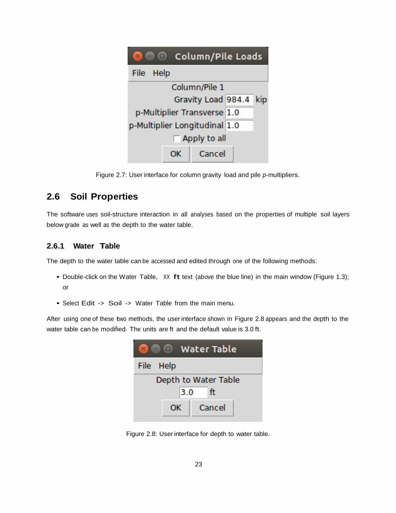
Figure 2.7: User interface for column gravity load and pile p-multipliers.
2.6 Soil Properties
The software uses soil-structure interaction in all analyses based on the properties of multiple soil layers below grade as well as the depth to the water table.
2.6.1 Water Table
The depth to the water table can be accessed and edited through one of the following methods:
• Double-click on the Water Table, XX ft text (above the blue line) in the main window (Figure 1.3); or
• Select Edit -> Soil -> Water Table from the main menu.
After using one of these two methods, the user interface shown in Figure 2.8 appears and the depth to the water table can be modified. The units are ft and the default value is 3.0 ft.
Figure 2.8: User interface for depth to water table.
23
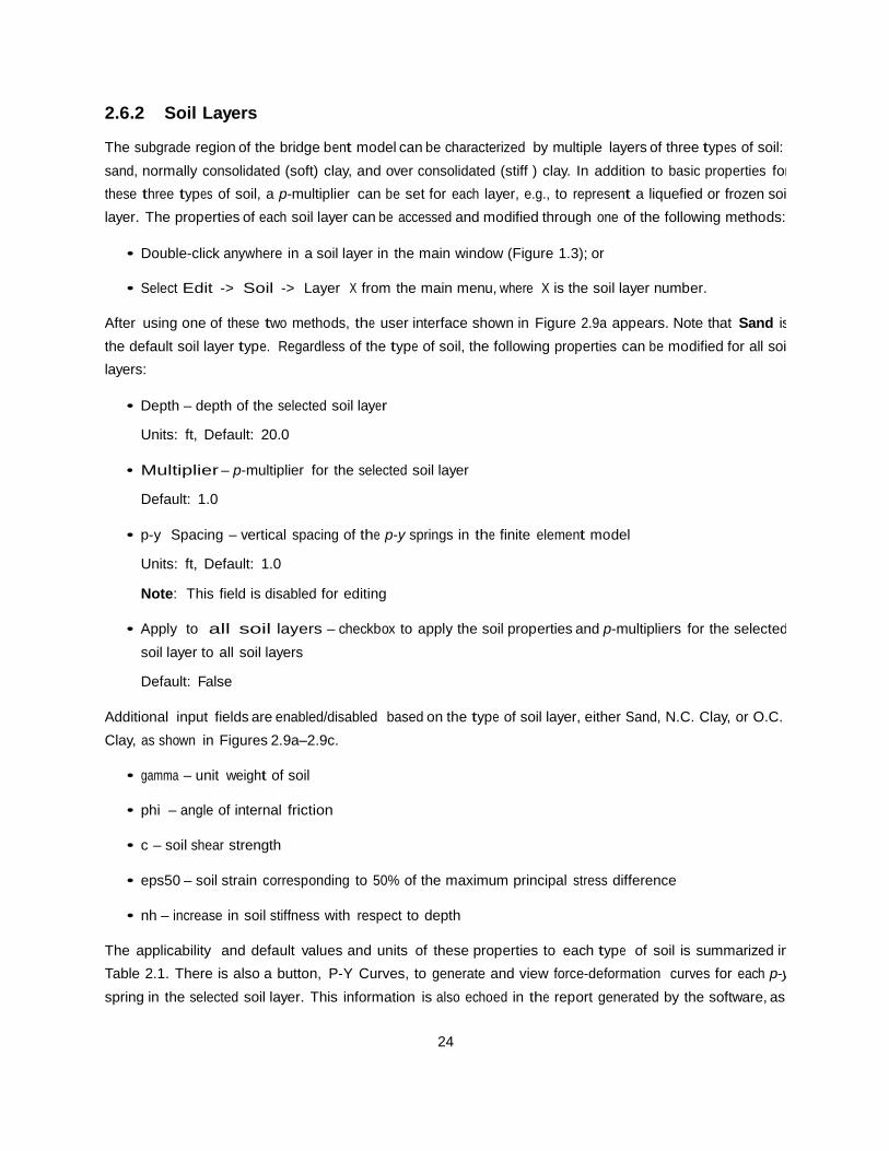
2.6.2 Soil Layers
The subgrade region of the bridge bent model can be characterized by multiple layers of three types of soil: sand, normally consolidated (soft) clay, and over consolidated (stiff ) clay. In addition to basic properties for these three types of soil, a p-multiplier can be set for each layer, e.g., to represent a liquefied or frozen soi layer. The properties of each soil layer can be accessed and modified through one of the following methods:
• Double-click anywhere in a soil layer in the main window (Figure 1.3); or
• Select Edit -> Soil -> Layer X from the main menu, where X is the soil layer number.
After using one of these two methods, the user interface shown in Figure 2.9a appears. Note that Sand is the default soil layer type. Regardless of the type of soil, the following properties can be modified for all soi layers:
• Depth – depth of the selected soil layer
Units: ft, Default: 20.0
• Multiplier – p-multiplier for the selected soil layer
Default: 1.0
• p-y Spacing – vertical spacing of the p-y springs in the finite element model
Units: ft, Default: 1.0
Note: This field is disabled for editing
• Apply to all soil layers – checkbox to apply the soil properties and p-multipliers for the selected soil layer to all soil layers
Default: False
Additional input fields are enabled/disabled based on the type of soil layer, either Sand, N.C. Clay, or O.C. Clay, as shown in Figures 2.9a–2.9c.
• gamma – unit weight of soil
• phi – angle of internal friction
• c – soil shear strength
• eps50 – soil strain corresponding to 50% of the maximum principal stress difference
• nh – increase in soil stiffness with respect to depth
The applicability and default values and units of these properties to each type of soil is summarized in Table 2.1. There is also a button, P-Y Curves, to generate and view force-deformation curves for each p-y spring in the selected soil layer. This information is also echoed in the report generated by the software, as
24
(a) Sand (Default). (b) Normally consolidated clay. (c) Over consolidated clay.
Figure 2.9: User interface for properties and p-multiplier of a soil layer.
described in Chapter 4, and will not be described here. The implementation of each of p-y soil model follows the procedures described in [12], with formulations developed by [10], [5], and [9] for O.C. clay, N.C. clay, and sand, respectively.
Table 2.1: Applicability of soil properties to sand, N.C. clay, and O.C. clay.
2.7 Saving the Bridge Model
The current properties of the bridge bent model can be saved to file by via one of the following approach:
• Type Ctrl + S in the main window (Figure 1.3)
25
Property Units Default Sand N.C. Clay O.C. Clay gamma pcf 125.0
phi deg 28.0 c psi 2.5
eps50 in/in 0.02 nh pci 50.0
X X X X
X X X X
X X
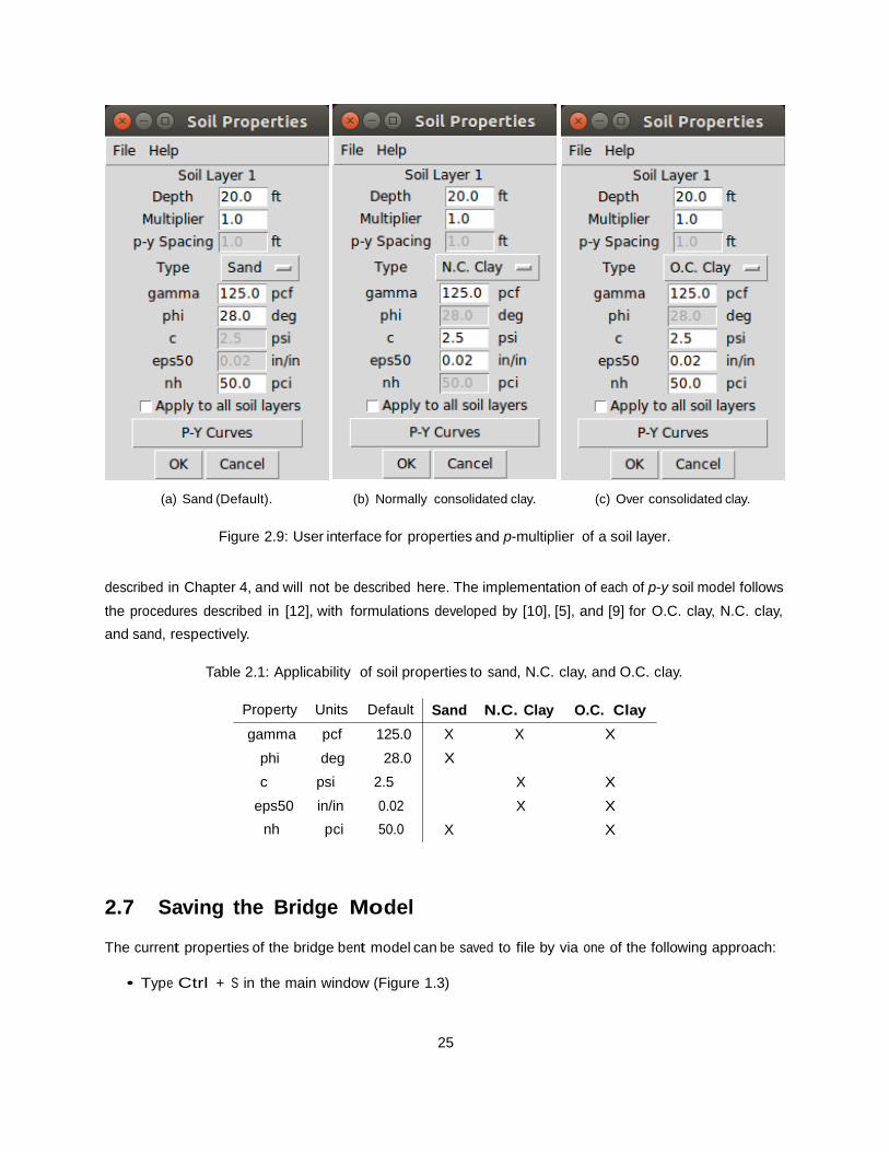
• Select File -> Save from the main menu
This will bring the dialog shown in Figure 2.10. The file extension for files saved by the software is .cis and the default file name for the bridge model is the bridge name.
Figure 2.10: Dialog to save a bridge bent model to file.
2.8 Loading a Bridge Model
A previously analyzed bridge bent model can be opened from file by via one of the following approach:
• Type Ctrl + O in the main window (Figure 1.3)
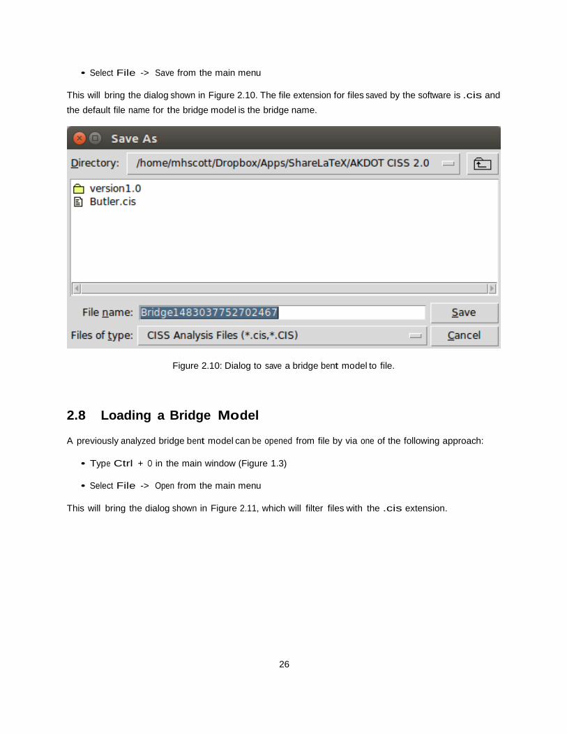
• Select File -> Open from the main menu This will bring the dialog shown in Figure 2.11, which will filter files with the .cis extension.
26
Figure 2.11: Dialog to load a bridge bent model from file.
27
Chapter 3
Finite Element Analysis
Using the bridge bent inputs for structural and soil properties described in Chapter 2, the software creates a two-dimensional (2D) nonlinear finite element model from modules available in OpenSees [6]. The model consists of frame (beam-column) and spring elements as described herein.
3.1 Boundary Conditions
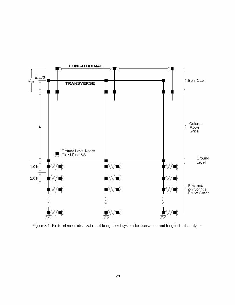
The element connectivity and boundary conditions of the bridge bent model are shown in Figure 3.1. The same model is used for transverse and longitudinal analyses with only one difference in the bent cap model For the transverse model, vertical bent cap elements extend from the top of the column to the mid-depth of the bent cap (dcap /2) with horizontal elastic frame elements connecting each column line, allowing for frame
action. For the longitudinal model, the vertical bent cap elements extend over the entire bent cap depth, dcap , with horizontal elastic truss elements (moment releases at each end) connecting each column line. This
removes frame action for the longitudinal analyses. Although longitudinal analyses can be accomplished with only one line of column/pile elements and no horizontal bent cap elements, this approach reduces programming complexity as essentially the same model is used for transverse and longitudinal analyses. The additional computational expense encumbered by this approach is minimal as this is a 2D finite element model with a relatively small number of nodes and elements.
At the base of each pile extension, a roller support prevents vertical displacement but allows rotation and horizontal displacement. The soil p-y springs provide the reaction forces that prevent rigid body dis- placement. If soil-structure interaction (SSI) effects are disabled in the analysis, the ground level nodes at the base of each column are completely fixed and will develop reaction forces. If SSI is disabled, the pile and p-y spring elements are not generated.
28
LONGITUDINAL
dcap Cap
Column ove de
Fixed if no SSI Ground Level
and Springs w Grade
Figure 3.1: Finite element idealization of bridge bent system for transverse and longitudinal analyses.
29
dcap/2
Bent TRANSVERSE
L
Ab Gra
Ground Level Nodes
1.0 ft 1.0 ft
Piles p-y Belo
3.2 Finite Element Formulations
The finite element formulations utilized in the 2D model shown in Figure 3.1 are as follows, along with the associated OpenSees element commands:
• Bent Cap – linear-elastic, small displacement elastic beam-column elements utilizing the Euler- Bernoulli beam theory
element forceBeamColumn with section Elastic at two Gauss-Legendre integration points and geom- Transf Linear geometric transformation; for a longitudinal analysis, element truss is used for the horizontal elements in the bent cap region
• Columns Above Grade – material nonlinear, large displacement beam-column elements utilizing the Euler-Bernoulli beam theory
element forceBeamColumn [7] with the HingeRadau integration rule [11] with fiber-discretized section Fiber cross-sections and geomTransf Corotational geometric transformation [2] (geomTransf Linear if the user does not select P -∆ effects); the gap section is used for the integration point at the top of the column while the steel shell section is used at all other integration points along the column height; the plastic hinge length at the top of the column is equal to that input by the user (see section 2.3)
• Piles Below Grade – material nonlinear, small displacement beam-column elements utilizing the Euler-Bernoulli beam theory
element dispBeamColumn with fiber-discretized section Fiber cross-sections at two Gauss-Legendre integration points and geomTransf Linear geometric transformation; the steel shell column cross-section is used for pile elements above the column/pile transition depth while the pile cross-section is used below this depth
• Soil Springs Below Grade – zero length p-y spring elements with one-dimensional (uniaxial) force- deformation response
element zeroLength with uniaxialMaterial response based on which of the three soil types the user selected for each layer; allowances for the buoyant weight of soil below the water table are also made if the user has selected this option
3.3 Analysis Options
The software offers the user control over some of the aforementioned analysis options through two interfaces.
3.3.1 Modeling Options
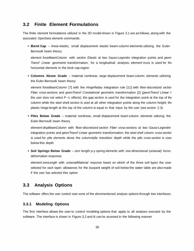
The first interface allows the user to control modeling options that apply to all analyses executed by the software. The interface is shown in Figure 3.2 and it can be accessed in the following manner
30
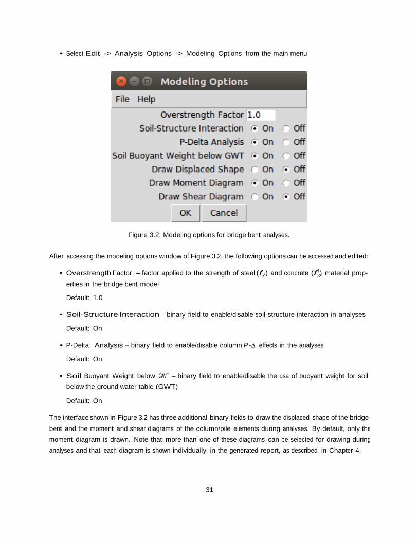
• Select Edit -> Analysis Options -> Modeling Options from the main menu
Figure 3.2: Modeling options for bridge bent analyses.
After accessing the modeling options window of Figure 3.2, the following options can be accessed and edited:
• Overstrength Factor – factor applied to the strength of steel (fy ) and concrete (f 1 ) material prop- c
erties in the bridge bent model Default: 1.0
• Soil-Structure Interaction – binary field to enable/disable soil-structure interaction in analyses
Default: On
• P-Delta Analysis – binary field to enable/disable column P -∆ effects in the analyses
Default: On
• Soil Buoyant Weight below GWT – binary field to enable/disable the use of buoyant weight for soil below the ground water table (GWT)
Default: On
The interface shown in Figure 3.2 has three additional binary fields to draw the displaced shape of the bridge bent and the moment and shear diagrams of the column/pile elements during analyses. By default, only the moment diagram is drawn. Note that more than one of these diagrams can be selected for drawing during analyses and that each diagram is shown individually in the generated report, as described in Chapter 4.
31
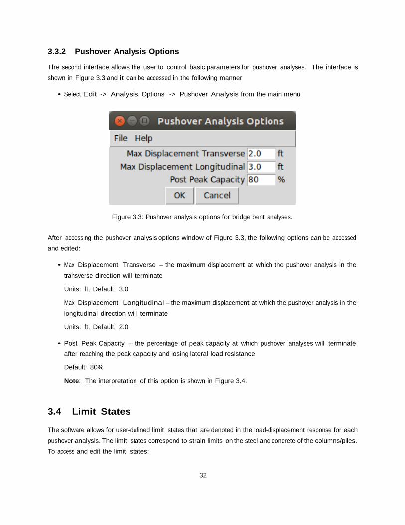
3.3.2 Pushover Analysis Options
The second interface allows the user to control basic parameters for pushover analyses. shown in Figure 3.3 and it can be accessed in the following manner
The interface is
• Select Edit -> Analysis Options -> Pushover Analysis from the main menu
Figure 3.3: Pushover analysis options for bridge bent analyses.
After accessing the pushover analysis options window of Figure 3.3, the following options can be accessed and edited:
• Max Displacement Transverse – the maximum displacement at which the pushover analysis in the transverse direction will terminate
Units: ft, Default: 3.0
Max Displacement Longitudinal – the maximum displacement at which the pushover analysis in the longitudinal direction will terminate
Units: ft, Default: 2.0
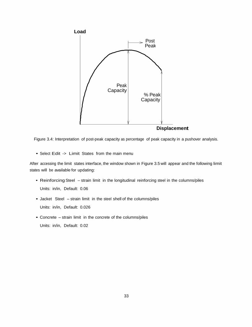
• Post Peak Capacity – the percentage of peak capacity at which pushover analyses will terminate after reaching the peak capacity and losing lateral load resistance
Default: 80%
Note: The interpretation of this option is shown in Figure 3.4.
3.4 Limit States
The software allows for user-defined limit states that are denoted in the load-displacement response for each pushover analysis. The limit states correspond to strain limits on the steel and concrete of the columns/piles. To access and edit the limit states:
32
Load
Peak
Capacity
Capacity
Displacement
Figure 3.4: Interpretation of post-peak capacity as percentage of peak capacity in a pushover analysis.
• Select Edit -> Limit States from the main menu
After accessing the limit states interface, the window shown in Figure 3.5 will appear and the following limit states will be available for updating:
• Reinforcing Steel – strain limit in the longitudinal reinforcing steel in the columns/piles
Units: in/in, Default: 0.06
• Jacket Steel – strain limit in the steel shell of the columns/piles
Units: in/in, Default: 0.026
• Concrete – strain limit in the concrete of the columns/piles
Units: in/in, Default: 0.02
33
Post
Peak
% Peak
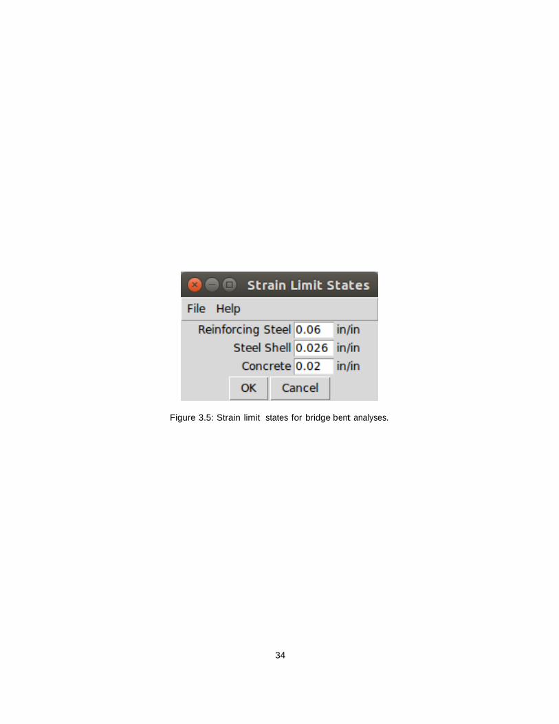
Figure 3.5: Strain limit states for bridge bent analyses.
34
Chapter 4
Summary Report
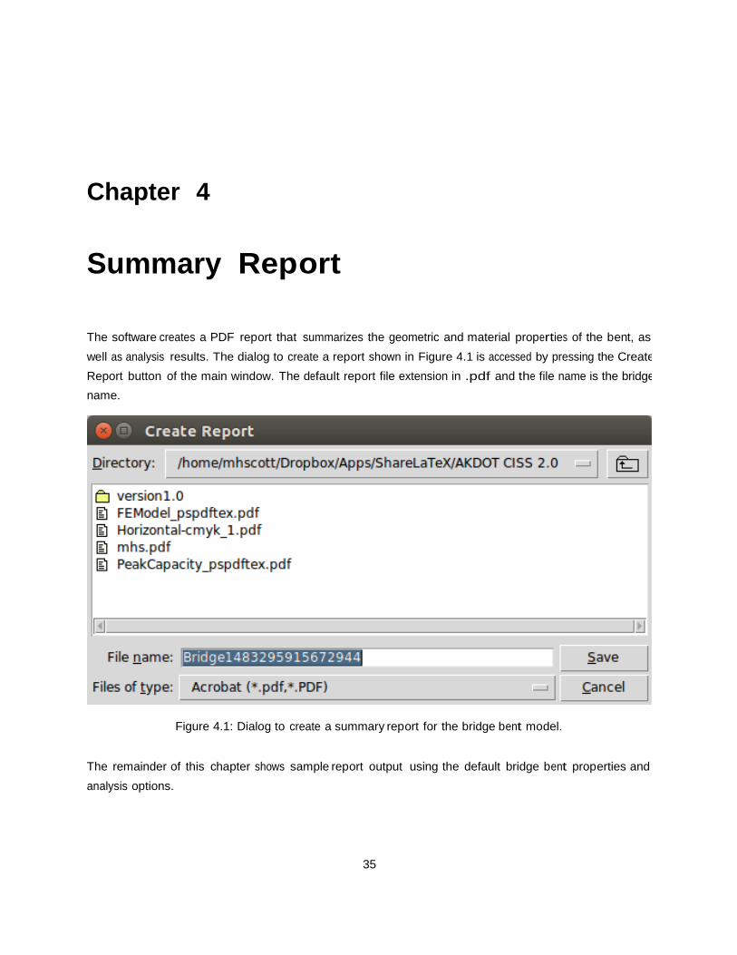
The software creates a PDF report that summarizes the geometric and material properties of the bent, as well as analysis results. The dialog to create a report shown in Figure 4.1 is accessed by pressing the Create Report button of the main window. The default report file extension in .pdf and the file name is the bridge name.
Figure 4.1: Dialog to create a summary report for the bridge bent model.
The remainder of this chapter shows sample report output using the default bridge bent properties and analysis options.
35
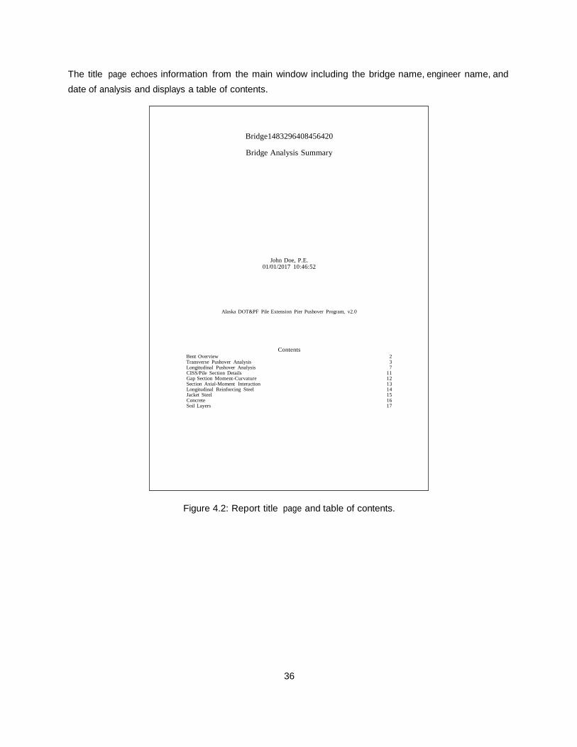
The title page echoes information from the main window including the bridge name, engineer name, and date of analysis and displays a table of contents.
Figure 4.2: Report title page and table of contents.
36
Bridge1483296408456420
Bridge Analysis Summary
John Doe, P.E. 01/01/2017 10:46:52
Alaska DOT&PF Pile Extension Pier Pushover Program, v2.0
Contents Bent Overview 2 Transverse Pushover Analysis 3 Longitudinal Pushover Analysis 7 CISS/Pile Section Details 11 Gap Section Moment-Curvature 12 Section Axial-Moment Interaction 13 Longitudinal Reinforcing Steel 14 Jacket Steel 15 Concrete 16 Soil Layers 17
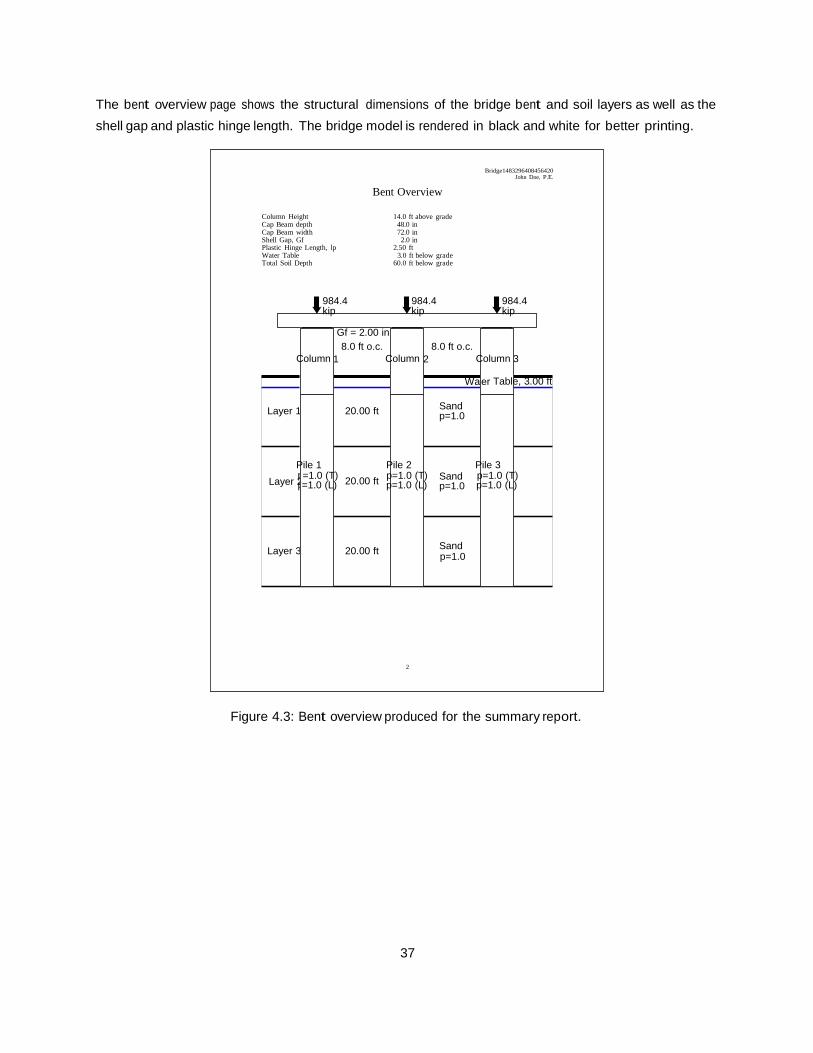
The bent overview page shows the structural dimensions of the bridge bent and soil layers as well as the shell gap and plastic hinge length. The bridge model is rendered in black and white for better printing.
Sand 20.00 ft =1.0 (L) p=1.0 (L) p=1.0 (L)
Figure 4.3: Bent overview produced for the summary report.
37
Bridge1483296408456420
John Doe, P.E.
Bent Overview
Column Height 14.0 ft above grade Cap Beam depth 48.0 in Cap Beam width 72.0 in Shell Gap, Gf 2.0 in Plastic Hinge Length, lp 2.50 ft Water Table 3.0 ft below grade Total Soil Depth 60.0 ft below grade
984.4 984.4 984.4 kip kip kip
Column Column Column
Table, 3.00 ft
p=1.0
Pile 1 Pile 2 Pile 3
=1.0 (T) p=1.0 (T) p=1.0 (T)
p=1.0
2
Gf = 2.00 in
8.0 ft o.c. 1
8.0 ft o.c.
2
3
Wat er
Layer 1
20.00 ft
Sand
p Layer 2p
p=1.0
Layer 3
20.00 ft
Sand
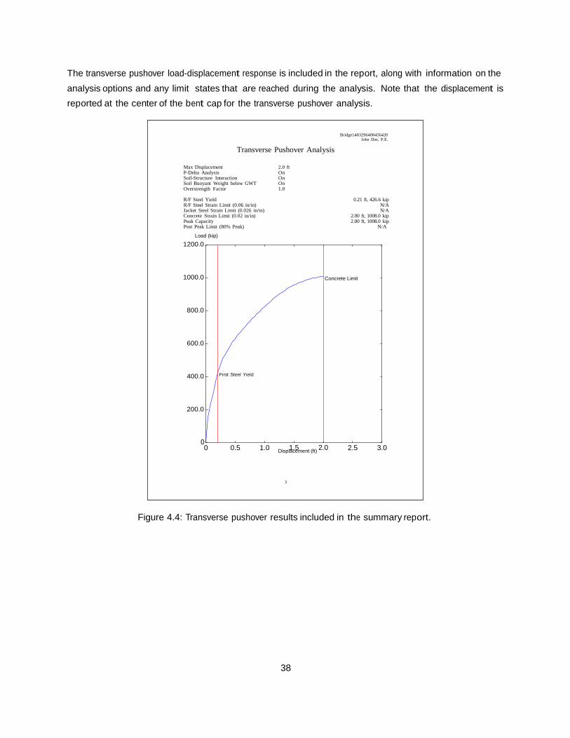
The transverse pushover load-displacement response is included in the report, along with information on the analysis options and any limit states that are reached during the analysis. reported at the center of the bent cap for the transverse pushover analysis.
Note that the displacement is
0 0.5 1.0 Displ1ac.5ement (ft) 2.0 2.5 3.0
Figure 4.4: Transverse pushover results included in the summary report.
38
Bridge1483296408456420
John Doe, P.E.
Transverse Pushover Analysis
Max Displacement 2.0 ft P-Delta Analysis On Soil-Structure Interaction On Soil Buoyant Weight below GWT On Overstrength Factor 1.0
R/F Steel Yield 0.21 ft, 426.6 kip R/F Steel Strain Limit (0.06 in/in) N/A Jacket Steel Strain Limit (0.026 in/in) N/A Concrete Strain Limit (0.02 in/in) 2.00 ft, 1008.0 kip Peak Capacity 2.00 ft, 1008.0 kip Post Peak Limit (80% Peak) N/A
Load (kip)
1200.0
1000.0
800.0
600.0
400.0
200.0
0
3
First Steel Yield
Concrete Limit
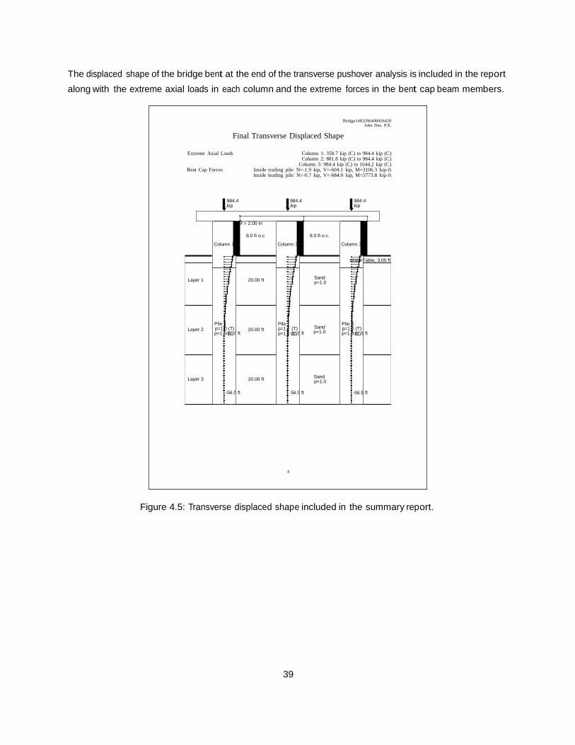
The displaced shape of the bridge bent at the end of the transverse pushover analysis is included in the report along with the extreme axial loads in each column and the extreme forces in the bent cap beam members.
kip kip kip
p=1.0 ft
Figure 4.5: Transverse displaced shape included in the summary report.
39
Bridge1483296408456420
John Doe, P.E.
Final Transverse Displaced Shape
Extreme Axial Loads Column 1: 358.7 kip (C) to 984.4 kip (C) Column 2: 881.8 kip (C) to 984.4 kip (C)
Column 3: 984.4 kip (C) to 1644.2 kip (C) Bent Cap Forces Inside trailing pile: N=-1.9 kip, V=-604.1 kip, M=3106.3 kip-ft
Inside leading pile: N=-0.7 kip, V=-684.0 kip, M=3773.8 kip-ft
984.4 984.4 984.4
Water
p=1.0
p=1.0 (T) p=1.0 (T)
p=1.0
4
Column 1
Gf = 2.00 in
8.0 ft o.c.
Column 2
8.0 ft o.c.
Column 3
Table, 3.00 ft
Layer 1
20.00 ft
Sand
Pile p=1.0 p=1.0
(T)
-3(L2).5 56.5
Pile
p=1.
1
0-3(L2).5 -56.5
Pile
p=1.
3
0-3(L2).5 -56.5
Layer 2
20.00 ft ft
ft
Sand
Layer 3
20.00 ft
ft
ft
Sand
ft
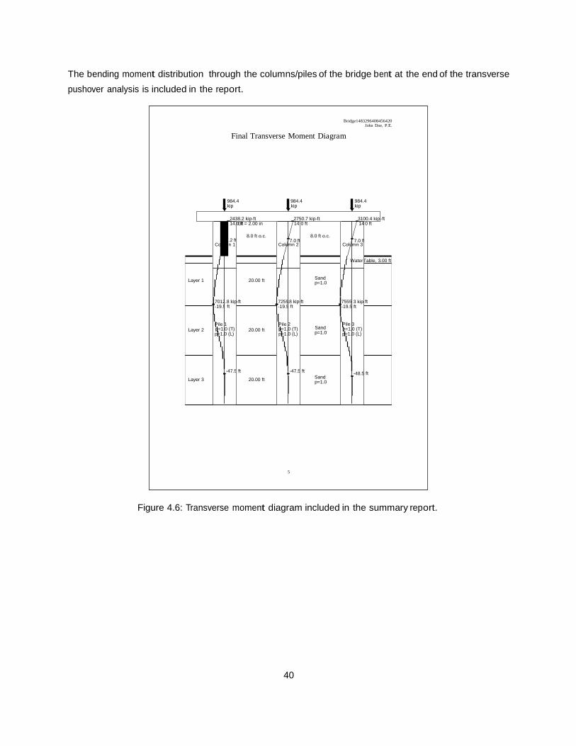
The bending moment distribution through the columns/piles of the bridge bent at the end of the transverse pushover analysis is included in the report.
kip kip kip
ft ft
p=1.0 (L) p=1.0 (L) p=1.0 (L)
Figure 4.6: Transverse moment diagram included in the summary report.
40
Bridge1483296408456420
John Doe, P.E.
Final Transverse Moment Diagram
984.4 984.4 984.4
Column 1 Column 2 Column 3
Water
p=1.0
.8 kip-ft .8 kip-ft ft
p=1.0 (T) p=1.0 (T) p=1.0 (T)
Sand
5
2438.2 kip-ft 2750.7 kip-ft 3100.4 kip -ft
14.
7.2 ft
0Gfft = 2.00 in
8.0 ft o.c.
14.
7.0 ft
0 ft
8.0 ft o.c.
14
7.0 ft
0 ft
Table, 3.00 ft
Layer 1
20.00 ft
Sand
1
-47.5
2
-47.5
7555 -19.5
Pile
3 kip- ft
3 -48.5
7012 -19.5
Pile
7259 -19.5
Pile
Layer 2
20.00 ft
Sand p=1.0
Layer 3
ft
20.00 ft
ft
ft
p=1.0
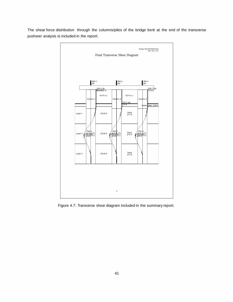
The shear force distribution through the columns/piles of the bridge bent at the end of the transverse pushover analysis is included in the report.
kip kip kip
p=1.0 1p.5=1ft.0 (L) 1p.5=1ft.0 (L) .0 (L) -3
Figure 4.7: Transverse shear diagram included in the summary report.
41
Bridge1483296408456420
John Doe, P.E.
Final Transverse Shear Diagram
984.4 984.4 984.4
Column 1 Column 2 Column 3
Water
p=1.0
419p.=21k. 428p.=81k.0 0p.=21k.i
p=1.0
6
334.1 kip 336.7 kip
G1f4=.02f.t00 in
8.0 ft o.c.
8.0 ft o.c.
337.2 kip
14.0 ft
0.0 ft Table, 3.00 ft
Layer 1
20.00 ft
Sand
Pile
1 0ip(T)
Pile
2 ip(T)
Pile
1p.5=1ft
3 0p (T)
Layer 2
-3
20.00 ft -3
Sand 44
Layer 3
20.00 ft
Sand
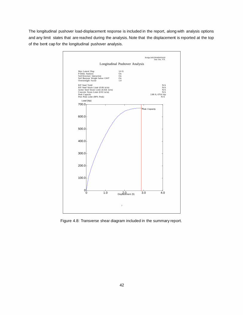
The longitudinal pushover load-displacement response is included in the report, along with analysis options and any limit states that are reached during the analysis. Note that the displacement is reported at the top of the bent cap for the longitudinal pushover analysis.
0 1.0 Displ2ac.0ement (ft) 3.0 4.0
Figure 4.8: Transverse shear diagram included in the summary report.
42
Bridge1483296408456420
John Doe, P.E.
Longitudinal Pushover Analysis
Max Lateral Disp 3.0 ft P-Delta Analysis On Soil-Structure Interaction On Soil Buoyant Weight below GWT On Overstrength Factor 1.0
R/F Steel Yield N/A R/F Steel Strain Limit (0.06 in/in) N/A Jacket Steel Strain Limit (0.026 in/in) N/A Concrete Strain Limit (0.02 in/in) N/A Peak Capacity 2.88 ft, 670.6 kip Post Peak Limit (80% Peak) N/A
Load (kip)
700.0
600.0
500.0
400.0
300.0
200.0
100.0
0
7
Peak Capacity
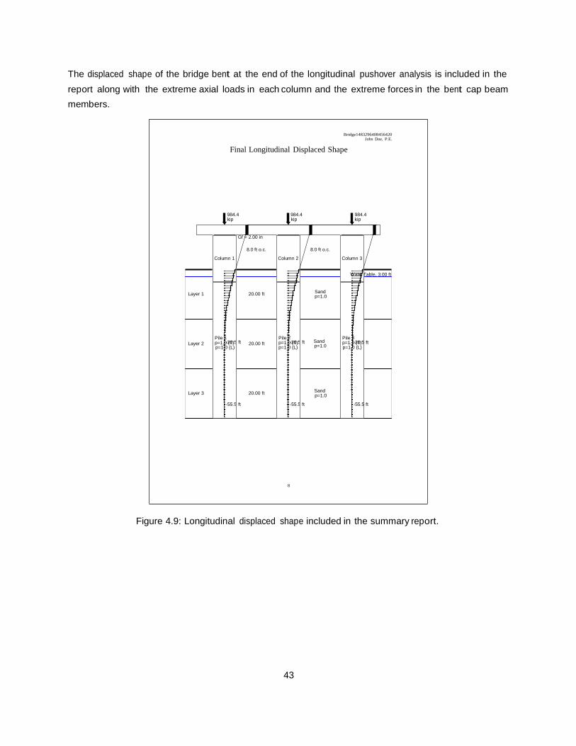
The displaced shape of the bridge bent at the end of the longitudinal pushover analysis is included in the report along with the extreme axial loads in each column and the extreme forces in the bent cap beam members.
kip kip kip
Figure 4.9: Longitudinal displaced shape included in the summary report.
43
Bridge1483296408456420
John Doe, P.E.
Final Longitudinal Displaced Shape
984.4 984.4 984.4
Water
p=1.0
p=1.0 (L) p=1.0 (L) p=1.0 p=1.0 (L)
p=1.0
8
Column 1
Gf = 2.00 in
8.0 ft o.c.
Column 2
8.0 ft o.c.
Column 3
Table, 3.00 ft
Layer 1
20.00 ft
Sand
Pile p=1.
1 0-3(T0).5
-55.5
Pile p=1.
2 0-3(T0).5
-55.5
Pile p=1.
3 0-3(T0).5
-55.5
Layer 2
ft 20.00 ft
ft
ft Sand
Layer 3
20.00 ft
ft
ft
Sand
ft

The bending moment distribution through the columns/piles of the bridge bent at the end of the longitudinal pushover analysis is included in the report.
kip kip kip
ft
p=1.0 (L) p=1.0 (L) p=1.0 (L)
Figure 4.10: Longitudinal moment diagram included in the summary report.
44
Bridge1483296408456420
John Doe, P.E.
Final Longitudinal Moment Diagram
984.4 984.4 984.4
lumn 1 lumn 2 lumn 3
Water
p=1.0
ft ft ft
p=1.0 (T) p=1.0 (T) p=1.0 (T)
176.8 kip-f2t 0.00 ft 176.8 kip-ft Sand 176.8 kip-ft
9
Co
Gf = 2.00 in
8.0 ft o.c.
Co
8.0 ft o.c.
Co
Table, 3.00 ft
Layer 1
20.00 ft
Sand
7687. -16.5
Pile
6 kip- ft
1 -50.5
7687. 16.5
Pile
6 kip- ft
2 -50.5
7687. -16.5
Pile
6 kip- 3 -50.5
Layer 2
20.00 ft
Sand p=1.0
Layer 3
ft
ft
ft p=1.0
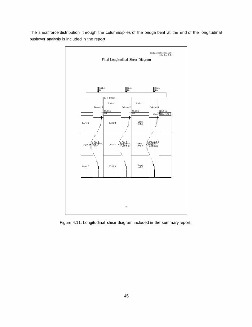
The shear force distribution through the columns/piles of the bridge bent at the end of the longitudinal pushover analysis is included in the report.
kip kip kip
0.0 ft Water
Sand 9p.5=1ft.0 (T) 9p.5=1ft.0 (T) -29p.5=1ft.0 (T)
Figure 4.11: Longitudinal shear diagram included in the summary report.
45
Bridge1483296408456420
John Doe, P.E.
Final Longitudinal Shear Diagram
984.4 984.4 984.4
Column 1 Column 2 Column 3
223.5 kip
p=1.0
6P.2ilek1 6P.2ilek2 6P.2ilek3 p=1.0
(L) p=1.0 (L) p=1.0 (L)
p=1.0
10
2
Gf = 2.00 in
8.0 ft o.c.
23.5 kip
2
8.0 ft o.c.
23.5 kip
0 .0 ft 0 .0 ft Table, 3.00 ft
Layer 1
20.00 ft
Sand
ip
ip
ip
43 Layer 2 -2
43 20.00 ft -2
43 p=1.0
Layer 3
20.00 ft
Sand
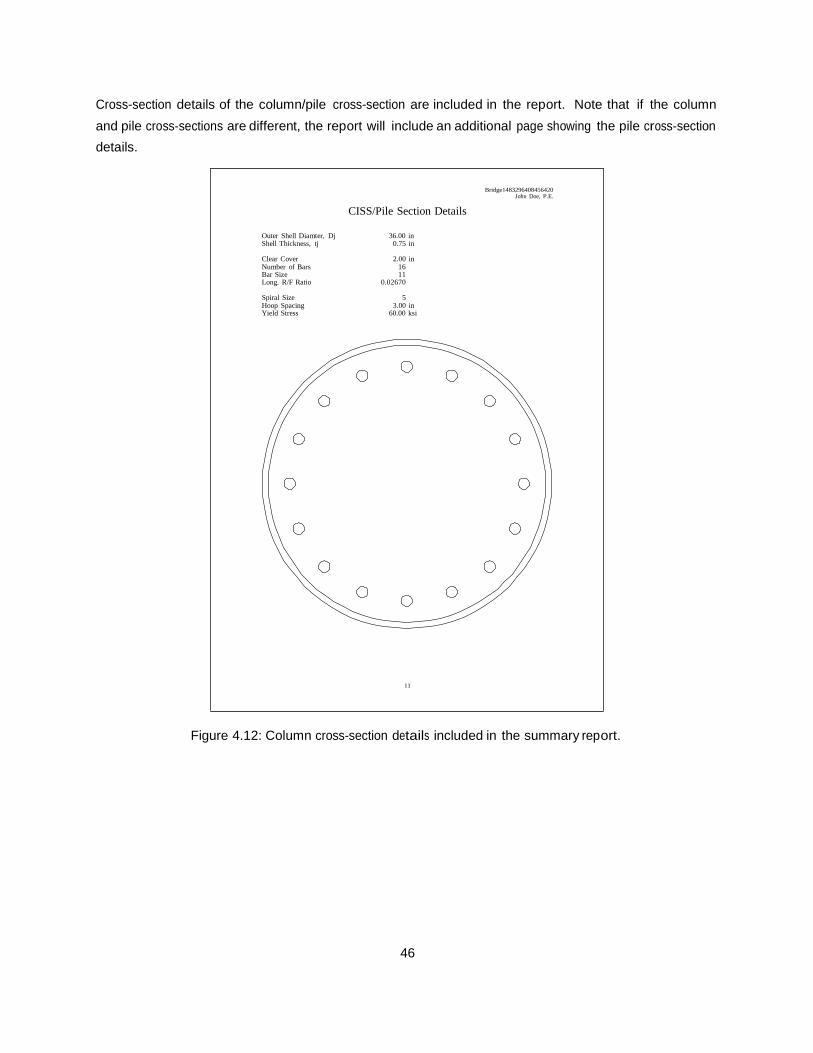
Cross-section details of the column/pile cross-section are included in the report. Note that if the column and pile cross-sections are different, the report will include an additional page showing the pile cross-section details.
Figure 4.12: Column cross-section details included in the summary report.
46
Bridge1483296408456420
John Doe, P.E.
CISS/Pile Section Details
Outer Shell Diamter, Dj 36.00 in Shell Thickness, tj 0.75 in
Clear Cover 2.00 in Number of Bars 16 Bar Size 11 Long. R/F Ratio 0.02670
Spiral Size 5 Hoop Spacing 3.00 in Yield Stress 60.00 ksi
11
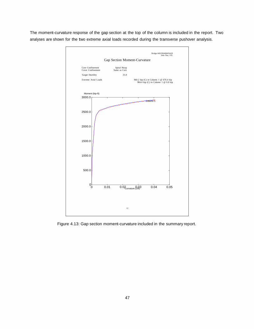
The moment-curvature response of the gap section at the top of the column is included in the report. Two analyses are shown for the two extreme axial loads recorded during the transverse pushover analysis.
0 0.01 0.02Curvature (01./f0t)3 0.04 0.05
Figure 4.13: Gap section moment-curvature included in the summary report.
47
Bridge1483296408456420
John Doe, P.E.
Gap Section Moment-Curvature
Core Confinement Spiral Hoop Cover Confinement Same as Core
Target Ductility 25.0
Extreme Axial Loads 960.2 kip (C) in Column 1 @ 670.4 kip
984.4 kip (C) in Column 1 @ 0.0 kip
Moment (kip-ft)
3000.0
2500.0
2000.0
1500.0
1000.0
500.0
0
12
Column 1
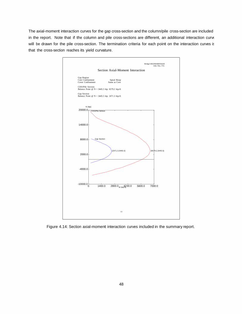
The axial-moment interaction curves for the gap cross-section and the column/pile cross-section are included in the report. Note that if the column and pile cross-sections are different, an additional interaction curve will be drawn for the pile cross-section. The termination criteria for each point on the interaction curves is that the cross-section reaches its yield curvature.
0 1400.0 2800.0 M (kip4-f2t) 00.0 5600.0 7000.0
Figure 4.14: Section axial-moment interaction curves included in the summary report.
48
Bridge1483296408456420
John Doe, P.E.
Section Axial-Moment Interaction
Gap Region Core Confinement Spiral Hoop Cover Confinement Same as Core
CISS/Pile Section Balance Point @ N = 3445.5 kip 6579.2 kip-ft
Gap Section Balance Point @ N = 3445.5 kip 2471.3 kip-ft
N (kip)
20000.0
14000.0
8000.0
(6579.2,3445.5)
2000.0
-4000.0
-10000.0
13
CISS/Pile Section
Gap Section
(2471.3,3445.5)

The stress-strain response curves of the longitudinal reinforcing steel and the steel shell are included in the report along with the material properties.
John Doe, P.E.
Yield Stress, fye
Strain-Hardening Onset, epssh
Rupture Strain, epssuR
60.0 ksi
0.0115 in/in
0.04 in/in
0 0.02 0.04 0.06 0.08 0.1
(a) Reinforcing steel. (b) Steel shell.
Figure 4.15: Steel stress-strain response included in the summary report.
49
Bridge1483296408456420
John Doe, P.E.
Longitudinal Reinforcing Steel
Elastic Modulus, E 29000.0 ksi Yield Stress, fye 68.0 ksi Ultimate Stress, fue 95.0 ksi Strain-Hardening Onset, epssh 0.0115 in/in Strain-Hardening Coefficient, C1 1.5 Rupture Strain, epssuR 0.06 in/in Ultimate Strain, epssu 0.09 in/in
Stress (ksi)
100.0
80.0
60.0
40.0
20.0
0 0 0.02 0.04 Strain (in/0in.)06 0.08 0.1
14
Bridge1483296408456420
Jacket Steel
Elastic Modulus, E 29000.0 ksi
Ultimate Stress, fue 78.0 ksi
Strain-Hardening Coefficient, C1 1.5
Ultimate Strain, epssu 0.06 in/in
Stress (ksi)
80.0
60.0
40.0
20.0
0 Strain (in/in)
15
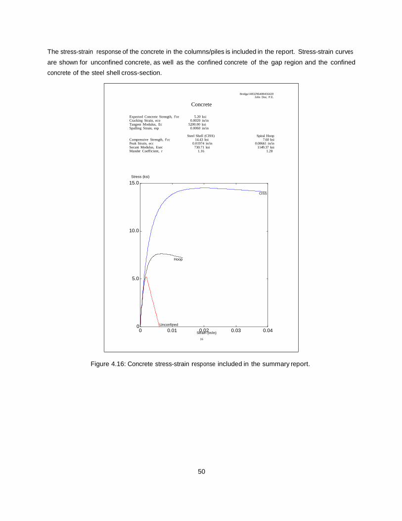
The stress-strain response of the concrete in the columns/piles is included in the report. Stress-strain curves are shown for unconfined concrete, as well as the confined concrete of the gap region and the confined concrete of the steel shell cross-section.
0 0.01 S0tra.0in2(in/in) 0.03 0.04
Figure 4.16: Concrete stress-strain response included in the summary report.
50
Bridge1483296408456420
John Doe, P.E.
Concrete
Expected Concrete Strength, f'ce 5.20 ksi Cracking Strain, eco 0.0020 in/in Tangent Modulus, Ec 5200.00 ksi Spalling Strain, esp 0.0060 in/in
Steel Shell (CISS) Spiral Hoop
Compressive Strength, f'cc 14.43 ksi 7.60 ksi Peak Strain, ecc 0.01974 in/in 0.00661 in/in Secant Modulus, Esec 730.71 ksi 1149.37 ksi Mander Coefficient, r 1.16 1.28
Stress (ksi)
15.0
10.0
5.0
0
16
CISS
Hoop
Unconfined
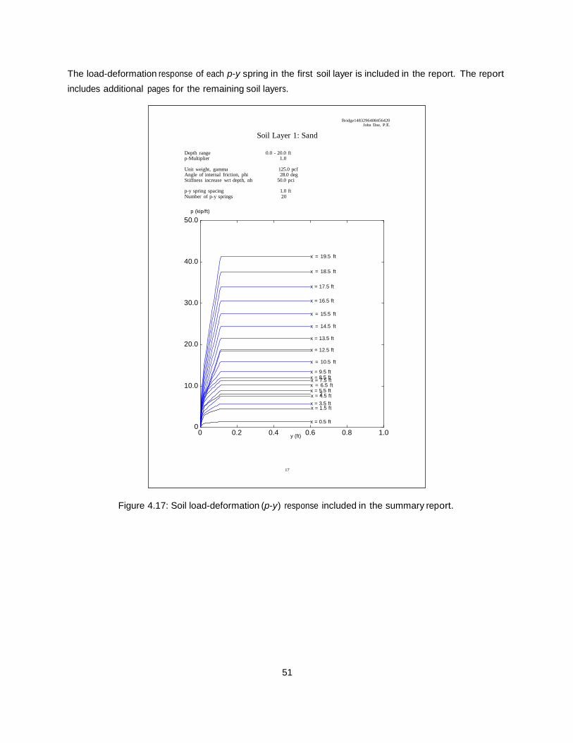
The load-deformation response of each p-y spring in the first soil layer is included in the report. The report includes additional pages for the remaining soil layers.
10.0
0 0.2 0.4 y (ft) 0.6 0.8 1.0
Figure 4.17: Soil load-deformation (p-y) response included in the summary report.
51
Bridge1483296408456420
John Doe, P.E.
Soil Layer 1: Sand
Depth range 0.0 - 20.0 ft p-Multiplier 1.0
Unit weight, gamma 125.0 pcf Angle of internal friction, phi 28.0 deg Stiffness increase wrt depth, nh 50.0 pci
p-y spring spacing 1.0 ft Number of p-y springs 20
p (kip/ft)
50.0
40.0
30.0
20.0
x = 7.5 ft
x = 24.5 ft
x = 1.5 ft
0
17
x = 19.5 ft
x = 18.5 ft
x = 17.5 ft
x = 16.5 ft
x = 15.5 ft
x = 14.5 ft
x = 13.5 ft
x = 12.5 ft
x = 10.5 ft
x = 9.5 ft x = 8.5 ft x = 6.5 ft x = 5.5 ft
x = 3.5 ft
x = 0.5 ft
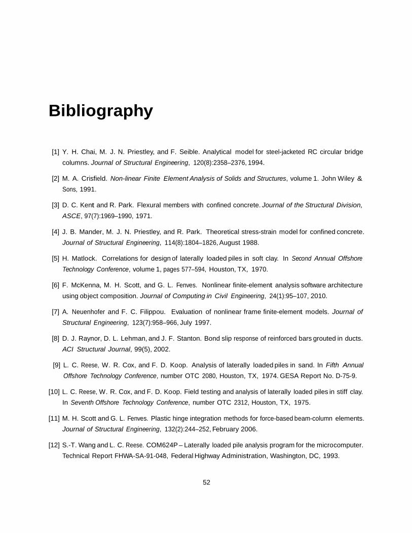
Bibliography
[1] Y. H. Chai, M. J. N. Priestley, and F. Seible. Analytical model for steel-jacketed RC circular bridge columns. Journal of Structural Engineering, 120(8):2358–2376, 1994.
[2] M. A. Crisfield. Non-linear Finite Element Analysis of Solids and Structures, volume 1. John Wiley & Sons, 1991.
[3] D. C. Kent and R. Park. Flexural members with confined concrete. Journal of the Structural Division, ASCE, 97(7):1969–1990, 1971.
[4] J. B. Mander, M. J. N. Priestley, and R. Park. Theoretical stress-strain model for confined concrete. Journal of Structural Engineering, 114(8):1804–1826, August 1988.
[5] H. Matlock. Correlations for design of laterally loaded piles in soft clay. In Second Annual Offshore Technology Conference, volume 1, pages 577–594, Houston, TX, 1970.
[6] F. McKenna, M. H. Scott, and G. L. Fenves. Nonlinear finite-element analysis software architecture using object composition. Journal of Computing in Civil Engineering, 24(1):95–107, 2010.
[7] A. Neuenhofer and F. C. Filippou. Evaluation of nonlinear frame finite-element models. Journal of Structural Engineering, 123(7):958–966, July 1997.
[8] D. J. Raynor, D. L. Lehman, and J. F. Stanton. Bond slip response of reinforced bars grouted in ducts. ACI Structural Journal, 99(5), 2002.
[9] L. C. Reese, W. R. Cox, and F. D. Koop. Analysis of laterally loaded piles in sand. In Fifth Annual Offshore Technology Conference, number OTC 2080, Houston, TX, 1974. GESA Report No. D-75-9.
[10] L. C. Reese, W. R. Cox, and F. D. Koop. Field testing and analysis of laterally loaded piles in stiff clay. In Seventh Offshore Technology Conference, number OTC 2312, Houston, TX, 1975.
[11] M. H. Scott and G. L. Fenves. Plastic hinge integration methods for force-based beam-column elements. Journal of Structural Engineering, 132(2):244–252, February 2006.
[12] S.-T. Wang and L. C. Reese. COM624P – Laterally loaded pile analysis program for the microcomputer. Technical Report FHWA-SA-91-048, Federal Highway Administration, Washington, DC, 1993.
52