An Adaptive Simplex Cut-Cell Method for Discontinuous ...kfid/pubs/Fidkowski_Darmofal_2007.pdfAn Adaptive Simplex Cut-Cell Method for Discontinuous Galerkin Discretizations of the

An Adaptive Simplex Cut-Cell Method for

Discontinuous Galerkin Discretizations of the

Navier-Stokes Equations

Krzysztof J. Fidkowski ∗

David L. Darmofal †

Massachusetts Institute of Technology, Cambridge, MA 02139

A cut-cell adaptive method is presented for high-order discontinuous Galerkin discretizations in

two and three dimensions. The computational mesh is constructed by cutting a curved geometry out

of a simplex background mesh that does not conform to the geometry boundary. The geometry is

represented with cubic splines in two dimensions and with a tesselation of quadratic patches in three

dimensions. High-order integration rules are derived for the arbitrarily-shaped areas and volumes

that result from the cutting. These rules take the form of quadrature-like points and weights that

are calculated in a pre-processing step. Accuracy of the cut-cell method is verified in both two and

three dimensions by comparison to boundary-conforming cases. The cut-cell method is also tested

in the context of output-based adaptation, in which an adjoint problem is solved to estimate the

error in an engineering output. Two-dimensional adaptive results for the compressible Navier-Stokes

equations illustrate automated anisotropic adaptation made possible by triangular cut-cell meshing.

In three dimensions, adaptive results for the compressible Euler equations using isotropic refinement

demonstrate the feasibility of automated meshing with tetrahedral cut cells and a curved geometry

representation. In addition, both the two and three-dimensional results indicate that, for the cases

tested, p = 2 and p = 3 solution approximation achieves the user-prescribed error tolerance more

efficiently compared to p = 1 and p = 0.

I. Introduction

Computational Fluid Dynamics (CFD) is used regularly in industry to reduce design cycle costs andto improve product design. The accessibility, relatively fast turnaround time, and almost arbitrary testconditions offered by CFD make it an attractive tool, especially for sensitivity studies, optimization, andpreliminary vehicle design. Although the use of CFD is prevalent, recent evidence suggests that it is not yet afully-mature field. In the most recent AIAA Drag Prediction Workshop (DPW), the spread in the on-designdrag values computed by some of the current state-of-the-art CFD codes was over 30 counts [1, 2]. Giventhat 1 drag count translates to several passengers for a typical long-range jet, such a spread is unacceptablefor engineering analysis and design.

The recent DPW results demonstrate that the risk of unacceptably large errors is high for current CFDpractices. Typically, such risks are managed by practitioners who are knowledgeable about the assumptionsand limitations of the models. However, even very experienced users cannot quantify the error in a discreteapproximation of a complex flowfield. As a result, current CFD practices are not robust across the widevariety of existing applications, including ones such as the DPW case, for which many of the codes are tuned.

Lack of automation is another key problem that plagues CFD analysis and design. Current industrypractices require heavy “person-in-the-loop” involvement, especially during mesh generation, which maytake days or weeks of user involvement and is often the bottleneck in CFD analysis. This meshing bottlenecknot only extends the design cycle time but also hinders the application of mesh adaptation methods anddesign optimization. Removing the user completely out of the design loop is neither possible nor advisable;

∗Research Assistant, Department of Aerospace Engineering, Building 37, Room 442. Student Member AIAA.†Associate Professor, Department of Aerospace Engineering, Building 37, Room 401. Senior Member AIAA.

1American Institute of Aeronautics and Astronautics

however, improving automation in areas such as meshing is expected to reduce design cycle time and toallow for techniques such as solution-based adaptation and optimization.

In an effort to improve the automation and robustness of CFD, this paper proposes a novel adaptive cut-cell method that uses a simplex (triangular/tetrahedral) background mesh and a high-order finite elementdiscretization. The motivation for cut cells is to remove the meshing bottleneck common to boundary-conforming methods: mesh generation is greatly simplified when the boundary of a complex geometry doesnot need to be taken into account. Removing this bottleneck then makes an automated adaptive solutionmethod possible.

The idea of using cut cells to automate meshing has been used successfully for finite volume discretizationson lattice-bound meshes [3–7]. These “Cartesian methods” differ from the present work in two ways. First,the present cut-cell method is applied to a high-order discontinuous Galerkin (DG) finite element method inwhich accurate volume as well as surface integrals need to be computed on irregularly-shaped regions. Theneed for high-order accuracy is motivated in previous works [8–10] in the interest of practical high-fidelityengineering calculations. Second, the use of simplex background mesh elements in the present work allowsfor anisotropic adaptation in general directions. Lack of such capability has been a roadblock in applyingCartesian methods to the Navier-Stokes equations.

The present work extends the two-dimensional cut-cell method presented in Ref. [11] into three dimen-sions, where the intersection and integration problems are of increased complexity. As this work is an initialproof-of-concept study, adaptation in three dimensions is performed with isotropic elements. Anisotropicresults are therefore only shown in two dimensions. The outline for the remainder of this paper is as follows.Section II describes the mechanics of intersecting a curved surface representation with a simplex backgroundmesh and the generation of high-order integration rules on the resulting irregular areas and volumes. SectionIII outlines the error estimation and mesh adaptation procedure. Section IV presents adaptive results in twoand three dimensions. Finally, Section V discusses conclusions and ongoing work.

II. Cut-cell Mesh Generation

A. Geometry Definition

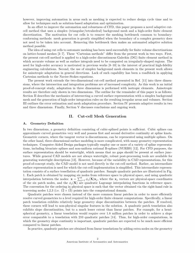
In two dimensions, a geometry definition consisting of cubic-splined points is sufficient. Cubic splines canapproximate curved geometries very well and possess first and second derivative continuity at spline knots.Geometric corners, where the tangent vector is discontinuous, can be represented using multiple splines. Onthe other hand, three-dimensional surface modeling is more complicated, with many geometry representationtechniques. Computer-Aided Design packages typically employ one or more of a variety of spline representa-tions, including bivariate splines and non-uniform rational B-splines (NURBS) [12]. For CFD purposes, thesurface representation should be watertight, which means that no gaps should be present at surface junc-tures. While general CAD models are not always watertight, robust post-processing tools are available forgenerating watertight descriptions [13]. However, because of the variability in CAD representations, for thisproof-of-concept study, the CAD model is not used directly in the cut-cell method. Rather, an intermediatesurface representation is used for which the cut-cell implementation is simplified. This intermediate represen-tation consists of a surface tessellation of quadratic patches. Sample quadratic patches are illustrated in Fig.1. Each patch is obtained by mapping six nodes from reference space to physical space, and using quadraticinterpolation between the nodes: x =

∑6

j=1 φj(X)xj , where the xj vectors are physical-space coordinatesof the six patch nodes, and the φj(X) are quadratic Lagrange interpolating functions in reference space.The convention for the ordering in physical space is such that the vector obtained via the right-hand rule intraversing nodes 1,2,3 (i.e. ~12 × ~13) points into the computational domain.

Quadratic patches were chosen instead of the more common linear patches in order to more efficientlyresolve curved geometries to a level required for high-order finite element computations. Specifically, a linearpatch tesselation exhibits relatively large geometry slope discontinuities between the patches. If resolved,these corners will lead to non-physical singular features in the solution. A quadratic patch tesselation alsoexhibits slope discontinuities, but to a much lesser extent than linear patches. For example, for a hemi-spherical geometry, a linear tesselation would require over 1.8 million patches in order to achieve a slopeerror comparable to a tesselation with 210 quadratic patches [14]. Thus, for high-order computations, inwhich the geometry slope continuity is important, quadratic patches are expected to be much more efficientcompared to linear patches.

In practice, quadratic patches are obtained from linear tesselations by adding extra nodes on the geometry


1

6

2

5

43

x

y

z

Figure 1. Two adjacent quadratic patches; the local node numbering for one of the patches is shown.

at the midpoints of the surface triangle edges. They are watertight because the interpolation of an edgedepends only on the locations of the three nodes on that edge, so that the surface interpolations from twoadjacent patches always match. While the nodes of the patches can be chosen to lie exactly on the geometry,the quadratically-interpolated coordinates of the patch interior and edges in general will not coincide with thegeometry. Thus, quadratic patches serve only as an approximation to the true geometry. A more accurate oreven exact geometry representation with tractable cut-cell intersection and integration algorithms is expectedto perform better and is an area of possible future work.

B. Cutting Algorithm

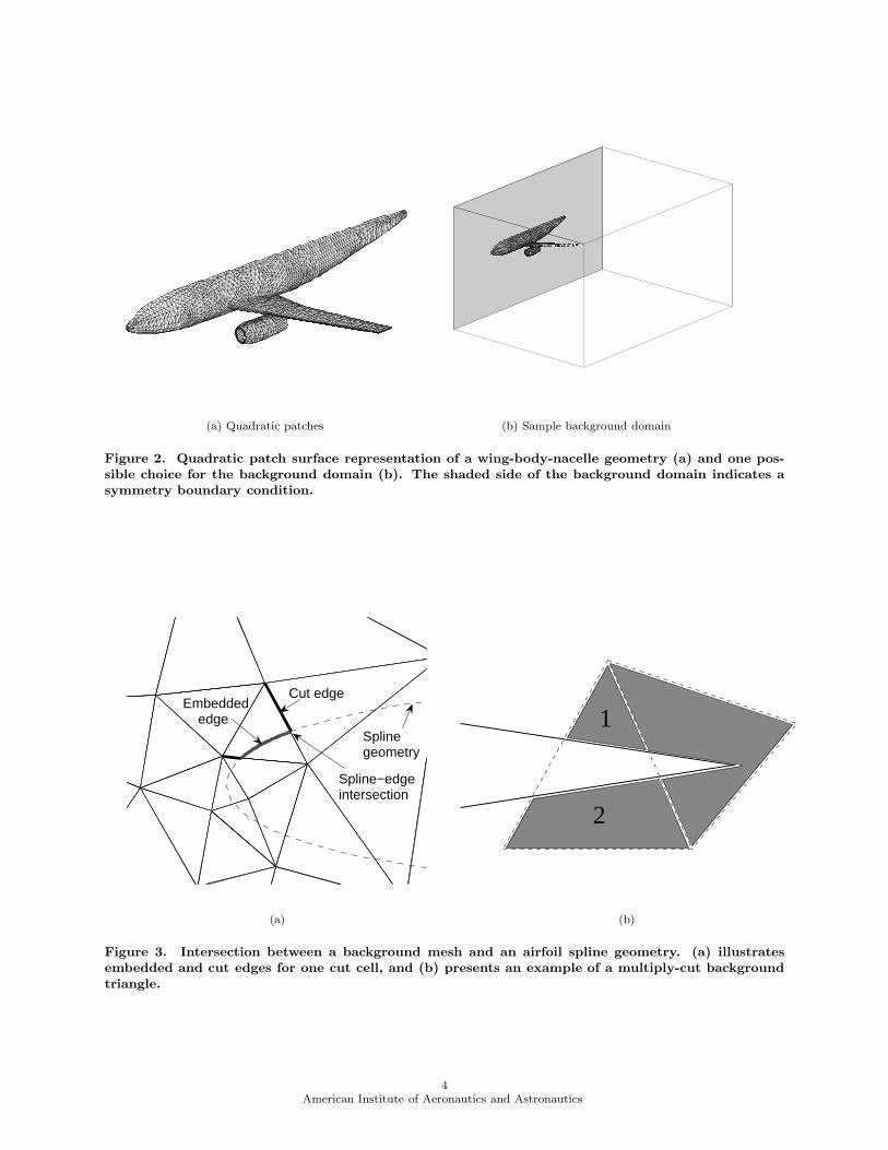
The cutting algorithm takes as input a spline or quadratic-patch surface representation of the geometry ofinterest and a linear area/volume mesh of the background domain. An example of a quadratic-patch surfacerepresentation of a wing-body-nacelle geometry is shown in Fig. 2a. Due to symmetry, only half of thegeometry is modeled. Shown in Fig. 2b is one possible choice for the background domain. In this case,it is a box; on five sides of the box, farfield boundary conditions are imposed, and the remaining side is asymmetry plane.

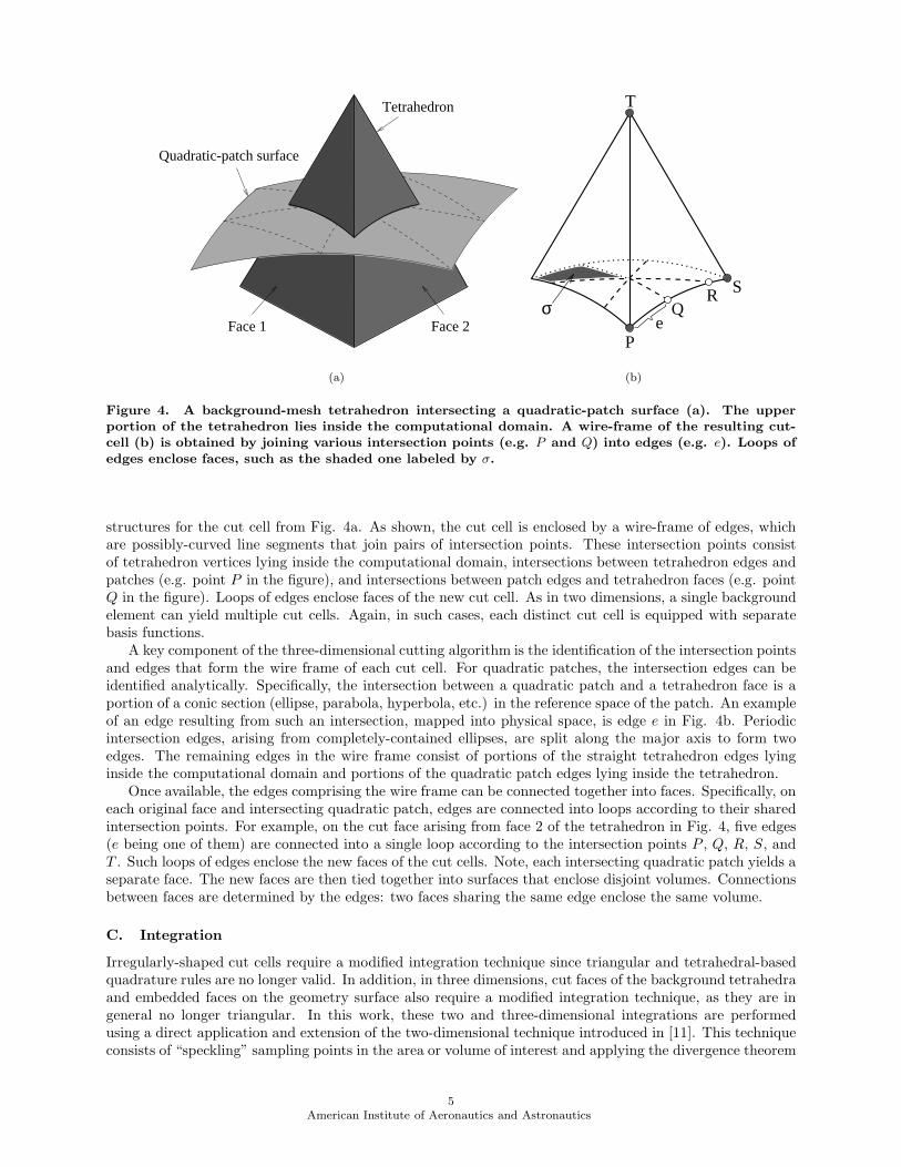
The output of the cutting algorithm is a cut-cell mesh of the computational domain obtained from theoriginal background mesh by removing elements completely contained in the geometry and by appropriatelycutting elements that intersect the geometry. The resulting cut cells are portions of the original trian-gles/tetrahedra that lie inside the computational domain. Fig. 3a illustrates a two-dimensional example inwhich a background mesh of triangles is cut by an airfoil spline geometry. An embedded edge and two cutedges are identified for one resulting cut cell. Embedded edges consist of contiguous portions of the splinegeometry inside the background mesh triangles, whereas cut edges consist of portions of background triangleedges inside the computational domain. Fig. 4a shows a three-dimensional example: an intersection betweena background-mesh tetrahedron and a quadratic patch surface. The upper portion of the tetrahedron liesinside the computational domain and forms a cut cell. Ultimately, for use in the solver, integration rules arerequired on the interior and on the boundary of each cut cell. However, generating these rules first requiresidentification and description of the intersections that produce the cut cells.

In two dimensions, the relevant intersections are between the cubic splines and the edges of the backgroundtriangles. These intersections are identified analytically by solving cubic equations. Each background trianglethus yields a set of embedded and cut edges that form the boundaries of the cut cells. Edges sharing commonintersections are joined into loops that enclose disjoint cut cells. Note, multiple cut cells arising from a singlebackground triangle are certainly possible, as shown in Fig. 3b for a triangle straddling an airfoil trailingedge. In such cases, each disjoint area is associated with a distinct cut cell equipped with separate sets ofpolynomial basis functions.

In three dimensions, the intersection problem is more complex. Figure 4b illustrates the basic intersection


(a) Quadratic patches (b) Sample background domain

Figure 2. Quadratic patch surface representation of a wing-body-nacelle geometry (a) and one pos-sible choice for the background domain (b). The shaded side of the background domain indicates asymmetry boundary condition.

Spline−edgeintersection

Splinegeometry

Cut edgeEmbedded edge

(a)

1

2

(b)

Figure 3. Intersection between a background mesh and an airfoil spline geometry. (a) illustratesembedded and cut edges for one cut cell, and (b) presents an example of a multiply-cut backgroundtriangle.


Face 2Face 1

Tetrahedron

Quadratic-patch surface

(a)

eP

σ QR S

T

(b)

Figure 4. A background-mesh tetrahedron intersecting a quadratic-patch surface (a). The upperportion of the tetrahedron lies inside the computational domain. A wire-frame of the resulting cut-cell (b) is obtained by joining various intersection points (e.g. P and Q) into edges (e.g. e). Loops ofedges enclose faces, such as the shaded one labeled by σ.

structures for the cut cell from Fig. 4a. As shown, the cut cell is enclosed by a wire-frame of edges, whichare possibly-curved line segments that join pairs of intersection points. These intersection points consistof tetrahedron vertices lying inside the computational domain, intersections between tetrahedron edges andpatches (e.g. point P in the figure), and intersections between patch edges and tetrahedron faces (e.g. pointQ in the figure). Loops of edges enclose faces of the new cut cell. As in two dimensions, a single backgroundelement can yield multiple cut cells. Again, in such cases, each distinct cut cell is equipped with separatebasis functions.

A key component of the three-dimensional cutting algorithm is the identification of the intersection pointsand edges that form the wire frame of each cut cell. For quadratic patches, the intersection edges can beidentified analytically. Specifically, the intersection between a quadratic patch and a tetrahedron face is aportion of a conic section (ellipse, parabola, hyperbola, etc.) in the reference space of the patch. An exampleof an edge resulting from such an intersection, mapped into physical space, is edge e in Fig. 4b. Periodicintersection edges, arising from completely-contained ellipses, are split along the major axis to form twoedges. The remaining edges in the wire frame consist of portions of the straight tetrahedron edges lyinginside the computational domain and portions of the quadratic patch edges lying inside the tetrahedron.

Once available, the edges comprising the wire frame can be connected together into faces. Specifically, oneach original face and intersecting quadratic patch, edges are connected into loops according to their sharedintersection points. For example, on the cut face arising from face 2 of the tetrahedron in Fig. 4, five edges(e being one of them) are connected into a single loop according to the intersection points P , Q, R, S, andT . Such loops of edges enclose the new faces of the cut cells. Note, each intersecting quadratic patch yields aseparate face. The new faces are then tied together into surfaces that enclose disjoint volumes. Connectionsbetween faces are determined by the edges: two faces sharing the same edge enclose the same volume.

C. Integration

Irregularly-shaped cut cells require a modified integration technique since triangular and tetrahedral-basedquadrature rules are no longer valid. In addition, in three dimensions, cut faces of the background tetrahedraand embedded faces on the geometry surface also require a modified integration technique, as they are ingeneral no longer triangular. In this work, these two and three-dimensional integrations are performedusing a direct application and extension of the two-dimensional technique introduced in [11]. This techniqueconsists of “speckling” sampling points in the area or volume of interest and applying the divergence theorem


��

��

��

��

��

��

��

��

��

��

��

��

��

��

��

��

Φ

x

x

(x )φ

φ

Bounding Box

(x , x )

(x )

1

1

0

0

1

0

(a) Tensor-product Lagrange functions, Φi(x)

Ray

Samplingpoint

��

��

��

��

��

��

��

��

��

��

��

��

��

��

��

��

��

��

��

��

��

��

��

��

Point offirst exit

(b) Sampling point selection

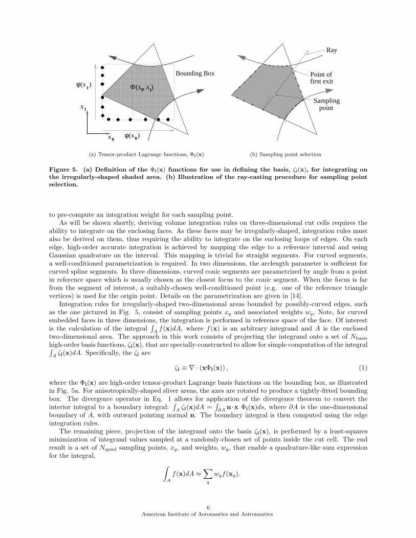
Figure 5. (a) Definition of the Φi(x) functions for use in defining the basis, ζi(x), for integrating onthe irregularly-shaped shaded area. (b) Illustration of the ray-casting procedure for sampling pointselection.

to pre-compute an integration weight for each sampling point.As will be shown shortly, deriving volume integration rules on three-dimensional cut cells requires the

ability to integrate on the enclosing faces. As these faces may be irregularly-shaped, integration rules mustalso be derived on them, thus requiring the ability to integrate on the enclosing loops of edges. On eachedge, high-order accurate integration is achieved by mapping the edge to a reference interval and usingGaussian quadrature on the interval. This mapping is trivial for straight segments. For curved segments,a well-conditioned parametrization is required. In two dimensions, the arclength parameter is sufficient forcurved spline segments. In three dimensions, curved conic segments are parametrized by angle from a pointin reference space which is usually chosen as the closest focus to the conic segment. When the focus is farfrom the segment of interest, a suitably-chosen well-conditioned point (e.g. one of the reference trianglevertices) is used for the origin point. Details on the parametrization are given in [14].

Integration rules for irregularly-shaped two-dimensional areas bounded by possibly-curved edges, suchas the one pictured in Fig. 5, consist of sampling points xq and associated weights wq, Note, for curvedembedded faces in three dimensions, the integration is performed in reference space of the face. Of interestis the calculation of the integral

∫

Af(x)dA, where f(x) is an arbitrary integrand and A is the enclosed

two-dimensional area. The approach in this work consists of projecting the integrand onto a set of Nbasis

high-order basis functions, ζi(x), that are specially-constructed to allow for simple computation of the integral∫

Aζi(x)dA. Specifically, the ζi are

ζi ≡ ∇ · (xΦi(x)) , (1)

where the Φi(x) are high-order tensor-product Lagrange basis functions on the bounding box, as illustratedin Fig. 5a. For anisotropically-shaped sliver areas, the axes are rotated to produce a tightly-fitted boundingbox. The divergence operator in Eq. 1 allows for application of the divergence theorem to convert theinterior integral to a boundary integral:

∫

Aζi(x)dA =

∫

∂An ·x Φi(x)ds, where ∂A is the one-dimensional

boundary of A, with outward pointing normal n. The boundary integral is then computed using the edgeintegration rules.

The remaining piece, projection of the integrand onto the basis ζi(x), is performed by a least-squaresminimization of integrand values sampled at a randomly-chosen set of points inside the cut cell. The endresult is a set of Nquad sampling points, xq, and weights, wq, that enable a quadrature-like sum expressionfor the integral,

∫

A

f(x)dA ≈∑

q

wqf(xq).


The weights are given by

wq = Qqj(R−T )ji

∫

A

ζi(x)dA, (2)

where ζi(xq) = QqjRji is a QR factorization and summation is implied on repeated indices. Since theexpression for wq does not involve the integrand, f(x), the weights can be calculated in a pre-processingstep and stored. The random sampling points, xq are determined by casting interior-bound rays from theenclosing edges and randomly chosing a point between the ray origin and the point of first exit. Thisprocedure is illustrated in Fig. 5b. To minimize the probability of an ill-conditioned set of sampling points,oversampling is used in which Nquad is set to 4Nbasis.

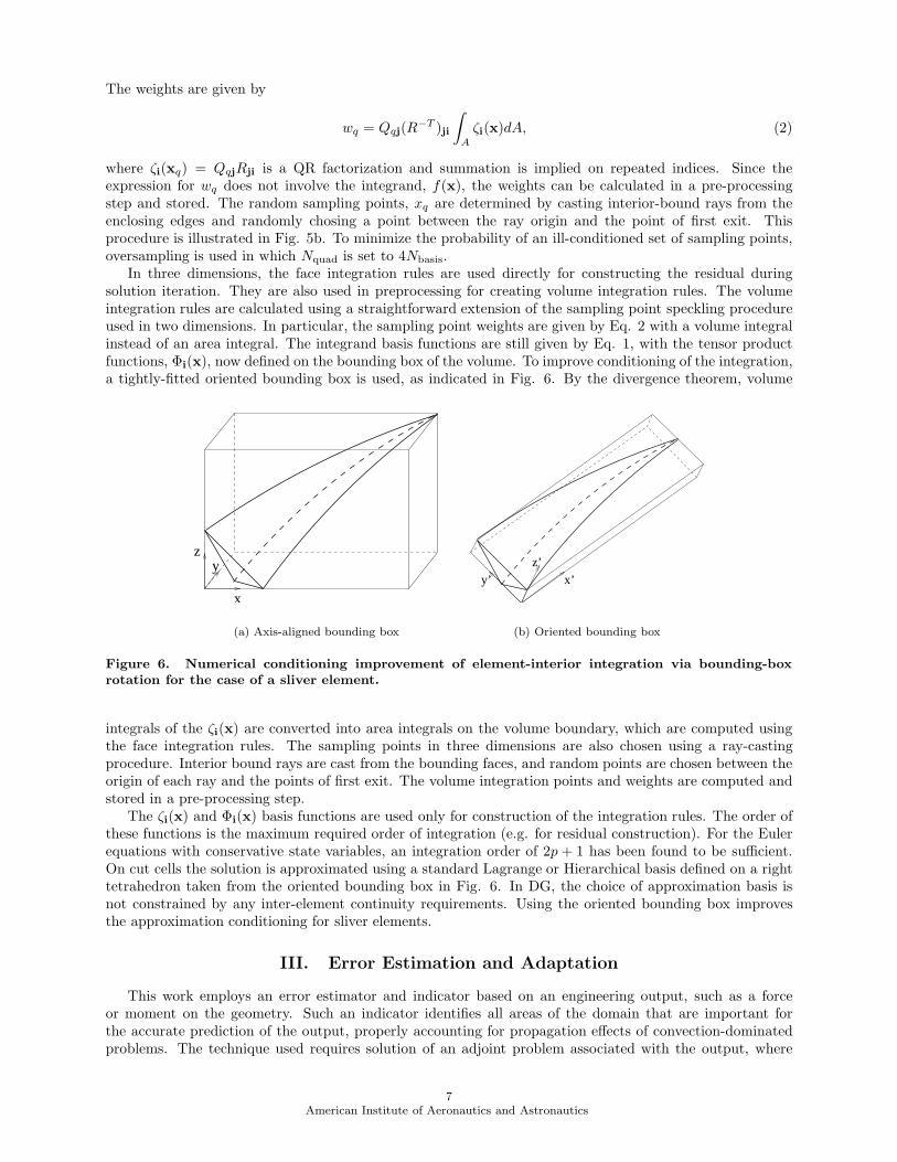
In three dimensions, the face integration rules are used directly for constructing the residual duringsolution iteration. They are also used in preprocessing for creating volume integration rules. The volumeintegration rules are calculated using a straightforward extension of the sampling point speckling procedureused in two dimensions. In particular, the sampling point weights are given by Eq. 2 with a volume integralinstead of an area integral. The integrand basis functions are still given by Eq. 1, with the tensor productfunctions, Φi(x), now defined on the bounding box of the volume. To improve conditioning of the integration,a tightly-fitted oriented bounding box is used, as indicated in Fig. 6. By the divergence theorem, volume

yz

x

(a) Axis-aligned bounding box

x’y’

z’

(b) Oriented bounding box

Figure 6. Numerical conditioning improvement of element-interior integration via bounding-boxrotation for the case of a sliver element.

integrals of the ζi(x) are converted into area integrals on the volume boundary, which are computed usingthe face integration rules. The sampling points in three dimensions are also chosen using a ray-castingprocedure. Interior bound rays are cast from the bounding faces, and random points are chosen between theorigin of each ray and the points of first exit. The volume integration points and weights are computed andstored in a pre-processing step.

The ζi(x) and Φi(x) basis functions are used only for construction of the integration rules. The order ofthese functions is the maximum required order of integration (e.g. for residual construction). For the Eulerequations with conservative state variables, an integration order of 2p + 1 has been found to be sufficient.On cut cells the solution is approximated using a standard Lagrange or Hierarchical basis defined on a righttetrahedron taken from the oriented bounding box in Fig. 6. In DG, the choice of approximation basis isnot constrained by any inter-element continuity requirements. Using the oriented bounding box improvesthe approximation conditioning for sliver elements.

III. Error Estimation and Adaptation

This work employs an error estimator and indicator based on an engineering output, such as a forceor moment on the geometry. Such an indicator identifies all areas of the domain that are important forthe accurate prediction of the output, properly accounting for propagation effects of convection-dominatedproblems. The technique used requires solution of an adjoint problem associated with the output, where


the adjoint links local residuals to the output error. This approach has been studied extensively in theliterature [15–21]. In particular, the error estimate used in this work is nearly identical to that used byHartmann and Houston and by Lu. On each element κ, the local error indicator is given by

ǫκ =1

2

∣

∣Rh(uH , (ψh −ψH)|κ)∣

∣ +1

2

∣

∣Rψh (uH ; (uh − uH)|κ,ψH)

∣

∣.

In the above expression, uH and ψH are the flow and adjoint solutions, and uh and ψh are higher-orderapproximations obtained via a patch-reconstruction of uH and ψH on an enriched, order p + 1 space. Rh

and Rψh are the flow and adjoint residuals evaluated on the enriched space, and |κ denotes restriction to

element κ. The global output error estimate, ǫ =∑

κ ǫκ, is not a bound on the actual error in the output;however, its validity is expected to increase as uH and ψH approach the exact solutions u and ψ.

Given a localized error estimate, an adaptive method modifies the computational mesh in an attemptto decrease and equidistribute the error. The adaptation strategy chosen for this work is h-adaptation at aconstant p. This strategy does not take advantage of the cost savings offered by hp-adaptation but avoids theadditional complexity involved in making the regularity estimation decision. This simplification also allowsfor a straightforward comparison of the adaptive performance at different interpolation orders. However,extension to hp-adaptation is one of the areas of possible future work.

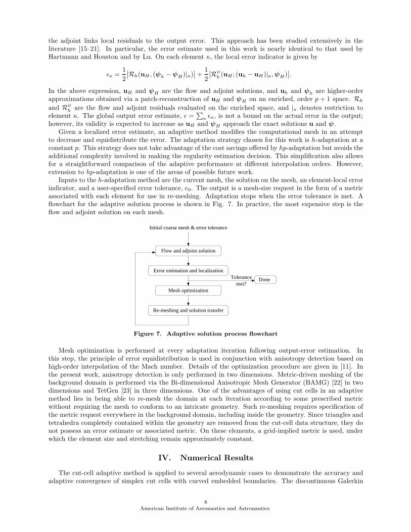
Inputs to the h-adaptation method are the current mesh, the solution on the mesh, an element-local errorindicator, and a user-specified error tolerance, e0. The output is a mesh-size request in the form of a metricassociated with each element for use in re-meshing. Adaptation stops when the error tolerance is met. Aflowchart for the adaptive solution process is shown in Fig. 7. In practice, the most expensive step is theflow and adjoint solution on each mesh.

Flow and adjoint solution

Initial coarse mesh & error tolerance

Error estimation and localization

Mesh optimization

Re-meshing and solution transfer

Tolerancemet?

Done

Figure 7. Adaptive solution process flowchart

Mesh optimization is performed at every adaptation iteration following output-error estimation. Inthis step, the principle of error equidistribution is used in conjunction with anisotropy detection based onhigh-order interpolation of the Mach number. Details of the optimization procedure are given in [11]. Inthe present work, anisotropy detection is only performed in two dimensions. Metric-driven meshing of thebackground domain is performed via the Bi-dimensional Anisotropic Mesh Generator (BAMG) [22] in twodimensions and TetGen [23] in three dimensions. One of the advantages of using cut cells in an adaptivemethod lies in being able to re-mesh the domain at each iteration according to some prescribed metricwithout requiring the mesh to conform to an intricate geometry. Such re-meshing requires specification ofthe metric request everywhere in the background domain, including inside the geometry. Since triangles andtetrahedra completely contained within the geometry are removed from the cut-cell data structure, they donot possess an error estimate or associated metric. On these elements, a grid-implied metric is used, underwhich the element size and stretching remain approximately constant.

IV. Numerical Results

The cut-cell adaptive method is applied to several aerodynamic cases to demonstrate the accuracy andadaptive convergence of simplex cut cells with curved embedded boundaries. The discontinuous Galerkin


discretization is applied to the compressible Navier-Stokes equations in two dimensions and to the Eulerequations in three dimensions. The Roe-averaged flux [24] is used for the inviscid term, and the second formof Bassi and Rebay [25] is used for the viscous term. The resulting non-linear system of equations is solvedvia a preconditioned Newton-GMRES technique [26].

Comparisons of the adapted meshes and the error convergence histories are given in terms of degrees offreedom (DOF) using interpolation orders p = 0 to p = 3 (p = 2 for three dimensions). The DOF countdoes not include the equation-specific multiplier, which is 4 in two dimensions and 5 in three dimensions. Inaddition, computational work estimates are given with the DOF results. The work estimate is of the formW ∼ Ne(n(p))a = DOF(n(p))a−1, where Ne is the number of elements, n(p) =

∏d

i=1(1 + p/i) is the DOFcount per element, and a is a measure of the computational complexity. From observations in practice, thework is assumed to be dominated by matrix-vector products, so that a ∼ 2.

A. Viscous flow over a NACA 0012 airfoil

In this case, a Navier-Stokes solution is computed around a NACA 0012 in a freestream Mach number of 0.5,Reynolds number of 5000, and angle of attack of 2o. The initial boundary-conforming and cut-cell meshesare isotropic and adapted to the geometry with roughly 250 elements. The farfield is a square, 100 chordlengths away from the airfoil. Mesh optimization is performed with anisotropic elements to efficiently resolvethe boundary layer and wake.

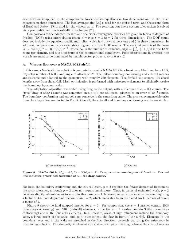
The adaptation algorithm was tested using drag as the output, with a tolerance of e0 = 0.1 counts. The“true” drag of 568.84 counts was computed on a p = 3 cut-cell mesh, adapted to an error of 10−3 counts.The boundary-conforming and cut-cell runs converge to the same drag value. The error convergence historiesfrom the adaptation are plotted in Fig. 8. Overall, the cut-cell and boundary-conforming results are similar.

103

104

105

10−2

10−1

100

101

102

103

DOF

Dra

g co

effic

ient

err

or, c

ount

s p = 1p = 2p = 3

(a) Boundary-conforming

103

104

105

10−2

10−1

100

101

102

103

DOF

Dra

g co

effic

ient

err

or, c

ount

s p = 1p = 2p = 3

(b) Cut-cell

Figure 8. NACA 0012: M∞ = 0.5, Re = 5000, α = 2o. Drag error versus degrees of freedom. Dashedline indicates prescribed tolerance of e0 = 0.1 drag counts.

For both the boundary-conforming and the cut-cell cases, p = 3 requires the fewest degrees of freedom atthe error tolerance, although p = 2 does not require much more. Thus, in terms of estimated work, p = 2becomes slightly advantageous to p = 3 in this case. p = 1, however, remains the most expensive, requiringa factor of 4-5 more degrees of freedom than p = 2, which translates to an estimated work increase of abouta factor of 2.

Figure 9 shows the final adapted meshes for p = 3. For comparison, the p = 2 meshes contain 4068(boundary-conforming) and 3403 (cut-cell) elements, while the p = 1 meshes contain 98808 (boundary-conforming) and 61163 (cut-cell) elements. In all meshes, areas of high refinement include the boundarylayer, a large extent of the wake, and, to a lesser extent, the flow in front of the airfoil. Elements in theboundary layer and in the wake are stretched in the flow direction, correctly capturing the anisotropy inthis viscous solution. The similarity in element size and anisotropic stretching between the cut-cell meshes


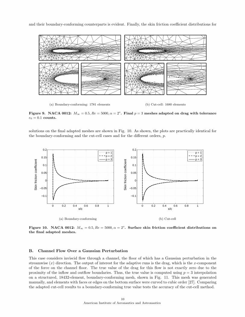
and their boundary-conforming counterparts is evident. Finally, the skin friction coefficient distributions for

(a) Boundary-conforming: 1781 elements (b) Cut-cell: 1680 elements

Figure 9. NACA 0012: M∞ = 0.5, Re = 5000, α = 2o. Final p = 3 meshes adapted on drag with tolerancee0 = 0.1 counts.

solutions on the final adapted meshes are shown in Fig. 10. As shown, the plots are practically identical forthe boundary-conforming and the cut-cell cases and for the different orders, p.

0 0.2 0.4 0.6 0.8 1

−0.1

−0.05

0

0.05

0.1

0.15

0.2

x/c

Ski

n fr

ictio

n co

effic

ient

p = 1p = 2p = 3

(a) Boundary-conforming

0 0.2 0.4 0.6 0.8 1

−0.1

−0.05

0

0.05

0.1

0.15

0.2

x/c

Ski

n fr

ictio

n co

effic

ient

p = 1p = 2p = 3

(b) Cut-cell

Figure 10. NACA 0012: M∞ = 0.5, Re = 5000, α = 2o. Surface skin friction coefficient distributions onthe final adapted meshes.

B. Channel Flow Over a Gaussian Perturbation

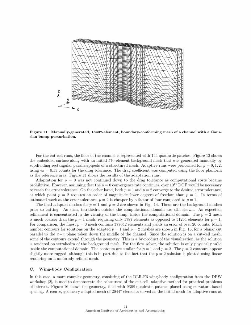
This case considers inviscid flow through a channel, the floor of which has a Gaussian perturbation in thestreamwise (x) direction. The output of interest for the adaptive runs is the drag, which is the x-componentof the force on the channel floor. The true value of the drag for this flow is not exactly zero due to theproximity of the inflow and outflow boundaries. Thus, the true value is computed using p = 3 interpolationon a structured, 18432-element, boundary-conforming mesh, shown in Fig. 11. This mesh was generatedmanually, and elements with faces or edges on the bottom surface were curved to cubic order [27]. Comparingthe adapted cut-cell results to a boundary-conforming true value tests the accuracy of the cut-cell method.


x

y

z

Figure 11. Manually-generated, 18432-element, boundary-conforming mesh of a channel with a Gaus-sian bump perturbation.

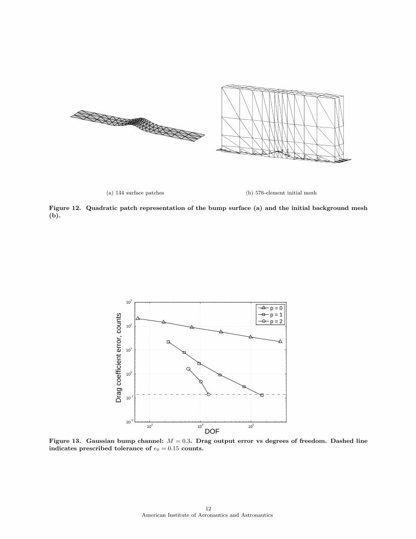
For the cut-cell runs, the floor of the channel is represented with 144 quadratic patches. Figure 12 showsthe embedded surface along with an initial 576-element background mesh that was generated manually bysubdividing rectangular parallelepipeds of a structured mesh. Adaptive runs were performed for p = 0, 1, 2,using e0 = 0.15 counts for the drag tolerance. The drag coefficient was computed using the floor planformas the reference area. Figure 13 shows the results of the adaptation runs.

Adaptation for p = 0 was not continued down to the drag tolerance as computational costs becameprohibitive. However, assuming that the p = 0 convergence rate continues, over 1010 DOF would be necessaryto reach the error tolerance. On the other hand, both p = 1 and p = 2 converge to the desired error tolerance,at which point p = 2 requires an order of magnitude fewer degrees of freedom than p = 1. In terms ofestimated work at the error tolerance, p = 2 is cheaper by a factor of four compared to p = 1.

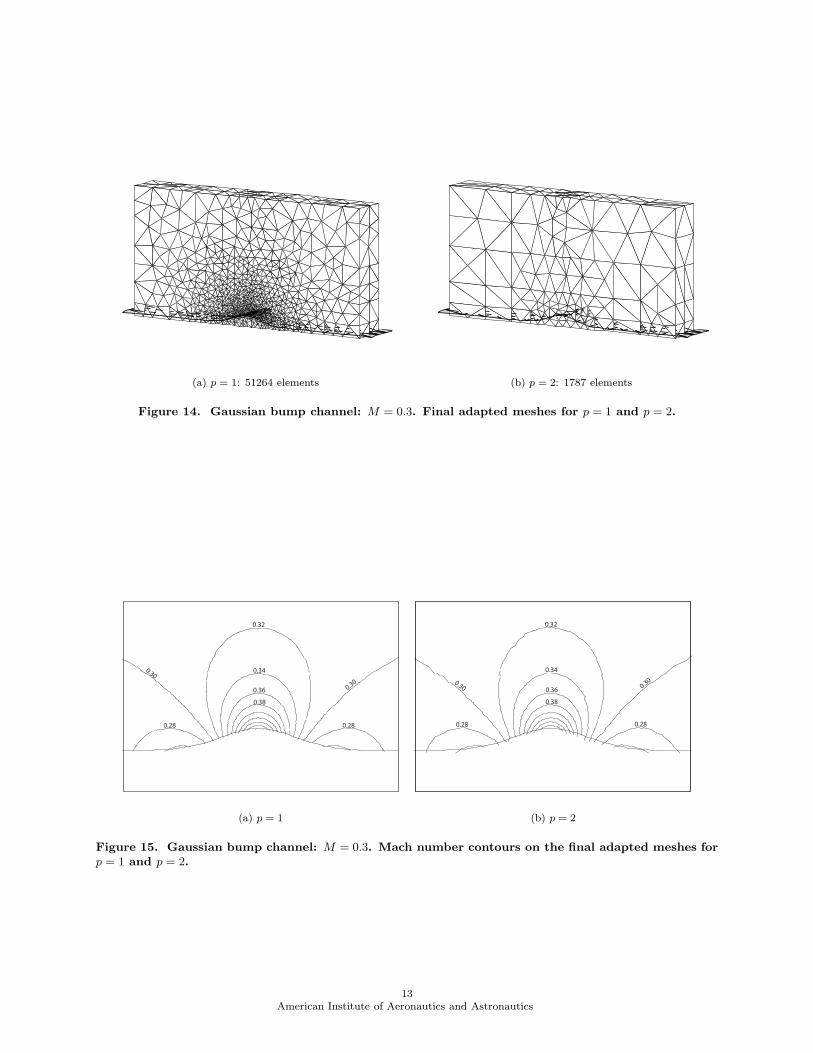
The final adapted meshes for p = 1 and p = 2 are shown in Fig. 14. These are the background meshesprior to cutting. As such, tetrahedra outside the computational domain are still shown. As expected,refinement is concentrated in the vicinity of the bump, inside the computational domain. The p = 2 meshis much coarser than the p = 1 mesh, requiring only 1787 elements as opposed to 51264 elements for p = 1.For comparison, the finest p = 0 mesh contains 377042 elements and yields an error of over 20 counts. Machnumber contours for solutions on the adapted p = 1 and p = 2 meshes are shown in Fig. 15, for a planar cutparallel to the x−z plane taken down the middle of the channel. Since the solution is on a cut-cell mesh,some of the contours extend through the geometry. This is a by-product of the visualization, as the solutionis rendered on tetrahedra of the background mesh. For the flow solver, the solution is only physically validinside the computational domain. The contours are similar for p = 1 and p = 2. The p = 2 contours appearslightly more rugged, although this is in part due to the fact that the p = 2 solution is plotted using linearrendering on a uniformly-refined mesh.

C. Wing-body Configuration

In this case, a more complex geometry, consisting of the DLR-F6 wing-body configuration from the DPWworkshop [2], is used to demonstrate the robustness of the cut-cell, adaptive method for practical problemsof interest. Figure 16 shows the geometry, tiled with 9368 quadratic patches placed using curvature-basedspacing. A coarse, geometry-adapted mesh of 20447 elements served as the initial mesh for adaptive runs at


(a) 144 surface patches (b) 576-element initial mesh

Figure 12. Quadratic patch representation of the bump surface (a) and the initial background mesh(b).

103

104

105

10−2

10−1

100

101

102

103

DOF

Dra

g co

effic

ient

err

or, c

ount

s

p = 0p = 1p = 2

Figure 13. Gaussian bump channel: M = 0.3. Drag output error vs degrees of freedom. Dashed lineindicates prescribed tolerance of e0 = 0.15 counts.


(a) p = 1: 51264 elements (b) p = 2: 1787 elements

Figure 14. Gaussian bump channel: M = 0.3. Final adapted meshes for p = 1 and p = 2.

0.32

0.300.34

0.36

0.38

0.28 0.28

0.30

(a) p = 1

0.32

0.34

0.36

0.38

0.28 0.28

0.30 0.30

(b) p = 2

Figure 15. Gaussian bump channel: M = 0.3. Mach number contours on the final adapted meshes forp = 1 and p = 2.


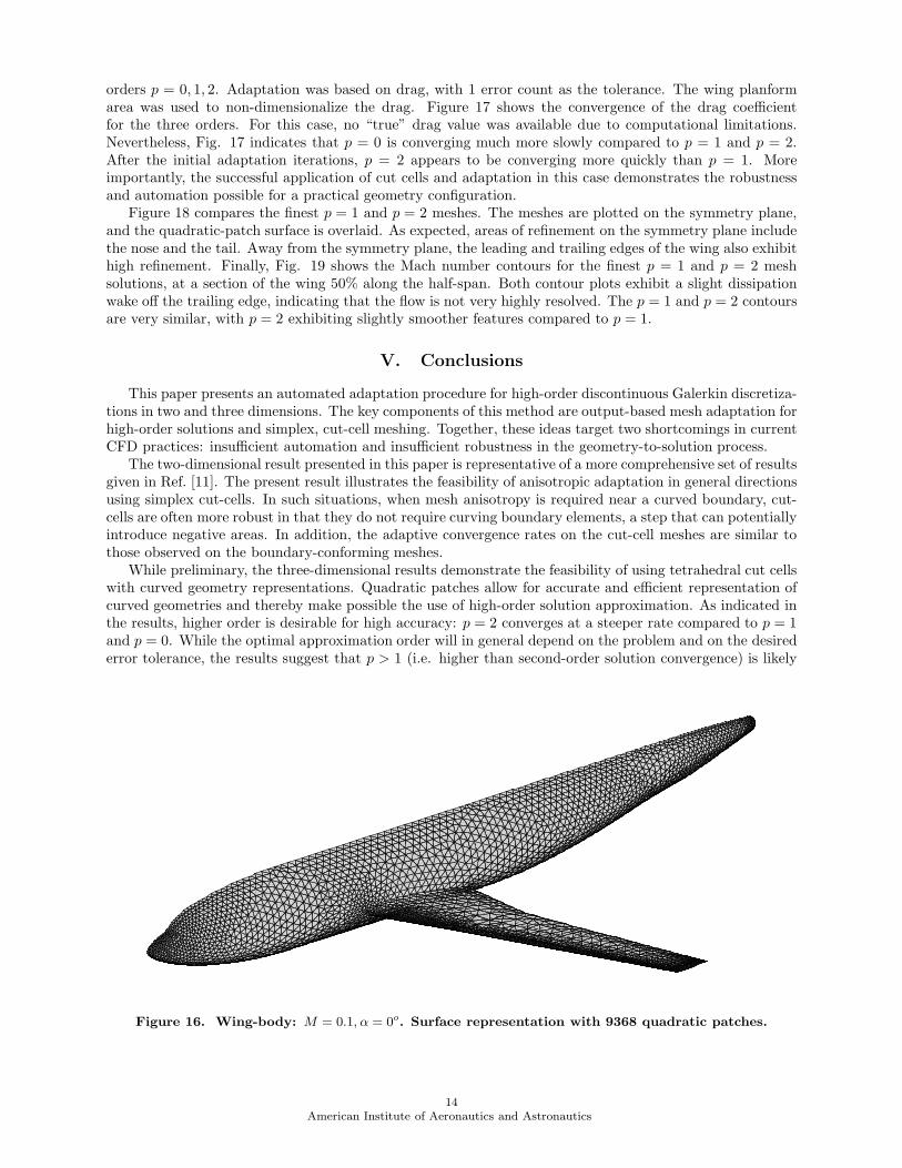
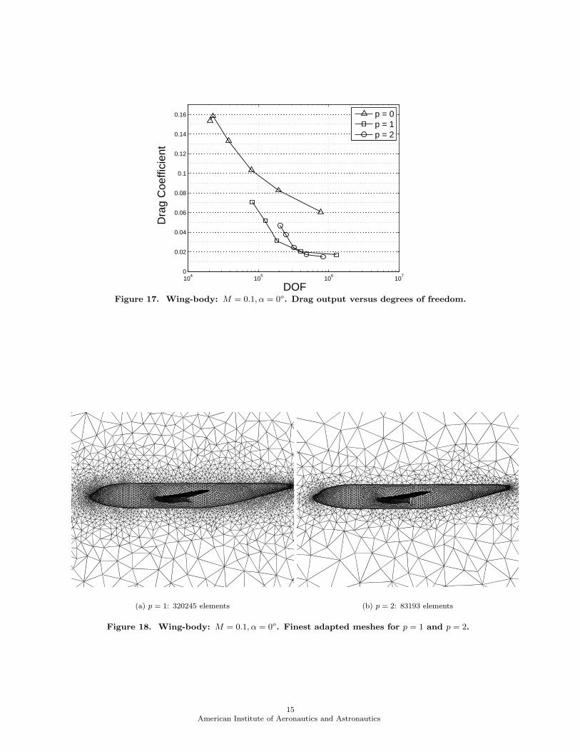
orders p = 0, 1, 2. Adaptation was based on drag, with 1 error count as the tolerance. The wing planformarea was used to non-dimensionalize the drag. Figure 17 shows the convergence of the drag coefficientfor the three orders. For this case, no “true” drag value was available due to computational limitations.Nevertheless, Fig. 17 indicates that p = 0 is converging much more slowly compared to p = 1 and p = 2.After the initial adaptation iterations, p = 2 appears to be converging more quickly than p = 1. Moreimportantly, the successful application of cut cells and adaptation in this case demonstrates the robustnessand automation possible for a practical geometry configuration.

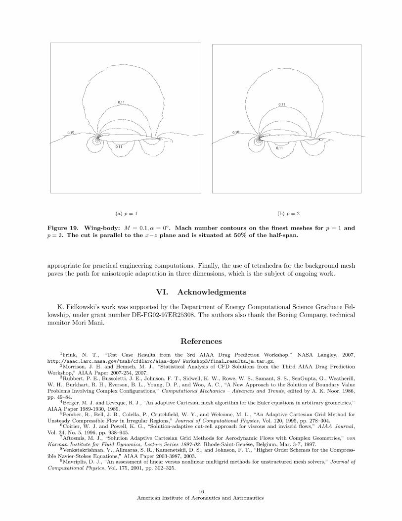
Figure 18 compares the finest p = 1 and p = 2 meshes. The meshes are plotted on the symmetry plane,and the quadratic-patch surface is overlaid. As expected, areas of refinement on the symmetry plane includethe nose and the tail. Away from the symmetry plane, the leading and trailing edges of the wing also exhibithigh refinement. Finally, Fig. 19 shows the Mach number contours for the finest p = 1 and p = 2 meshsolutions, at a section of the wing 50% along the half-span. Both contour plots exhibit a slight dissipationwake off the trailing edge, indicating that the flow is not very highly resolved. The p = 1 and p = 2 contoursare very similar, with p = 2 exhibiting slightly smoother features compared to p = 1.

V. Conclusions

This paper presents an automated adaptation procedure for high-order discontinuous Galerkin discretiza-tions in two and three dimensions. The key components of this method are output-based mesh adaptation forhigh-order solutions and simplex, cut-cell meshing. Together, these ideas target two shortcomings in currentCFD practices: insufficient automation and insufficient robustness in the geometry-to-solution process.

The two-dimensional result presented in this paper is representative of a more comprehensive set of resultsgiven in Ref. [11]. The present result illustrates the feasibility of anisotropic adaptation in general directionsusing simplex cut-cells. In such situations, when mesh anisotropy is required near a curved boundary, cut-cells are often more robust in that they do not require curving boundary elements, a step that can potentiallyintroduce negative areas. In addition, the adaptive convergence rates on the cut-cell meshes are similar tothose observed on the boundary-conforming meshes.

While preliminary, the three-dimensional results demonstrate the feasibility of using tetrahedral cut cellswith curved geometry representations. Quadratic patches allow for accurate and efficient representation ofcurved geometries and thereby make possible the use of high-order solution approximation. As indicated inthe results, higher order is desirable for high accuracy: p = 2 converges at a steeper rate compared to p = 1and p = 0. While the optimal approximation order will in general depend on the problem and on the desirederror tolerance, the results suggest that p > 1 (i.e. higher than second-order solution convergence) is likely

Figure 16. Wing-body: M = 0.1, α = 0o. Surface representation with 9368 quadratic patches.


104

105

106

107

0

0.02

0.04

0.06

0.08

0.1

0.12

0.14

0.16

DOF

Dra

g C

oeffi

cien

t

p = 0p = 1p = 2

Figure 17. Wing-body: M = 0.1, α = 0o. Drag output versus degrees of freedom.

(a) p = 1: 320245 elements (b) p = 2: 83193 elements

Figure 18. Wing-body: M = 0.1, α = 0o. Finest adapted meshes for p = 1 and p = 2.


0.10

0.11

0.11

(a) p = 1

0.11

0.11

0.10

(b) p = 2

Figure 19. Wing-body: M = 0.1, α = 0o. Mach number contours on the finest meshes for p = 1 andp = 2. The cut is parallel to the x−z plane and is situated at 50% of the half-span.

appropriate for practical engineering computations. Finally, the use of tetrahedra for the background meshpaves the path for anisotropic adaptation in three dimensions, which is the subject of ongoing work.

VI. Acknowledgments

K. Fidkowski’s work was supported by the Department of Energy Computational Science Graduate Fel-lowship, under grant number DE-FG02-97ER25308. The authors also thank the Boeing Company, technicalmonitor Mori Mani.

References

1Frink, N. T., “Test Case Results from the 3rd AIAA Drag Prediction Workshop,” NASA Langley, 2007,http://aaac.larc.nasa.gov/tsab/cfdlarc/aiaa-dpw/ Workshop3/final results jm.tar.gz.

2Morrison, J. H. and Hemsch, M. J., “Statistical Analysis of CFD Solutions from the Third AIAA Drag PredictionWorkshop,” AIAA Paper 2007-254, 2007.

3Rubbert, P. E., Bussoletti, J. E., Johnson, F. T., Sidwell, K. W., Rowe, W. S., Samant, S. S., SenGupta, G., Weatherill,W. H., Burkhart, R. H., Everson, B. L., Young, D. P., and Woo, A. C., “A New Approach to the Solution of Boundary ValueProblems Involving Complex Configurations,” Computational Mechanics – Advances and Trends, edited by A. K. Noor, 1986,pp. 49–84.

4Berger, M. J. and Leveque, R. J., “An adaptive Cartesian mesh algorithm for the Euler equations in arbitrary geometries,”AIAA Paper 1989-1930, 1989.

5Pember, R., Bell, J. B., Colella, P., Crutchfield, W. Y., and Welcome, M. L., “An Adaptive Cartesian Grid Method forUnsteady Compressible Flow in Irregular Regions,” Journal of Computational Physics, Vol. 120, 1995, pp. 278–304.

6Coirier, W. J. and Powell, K. G., “Solution-adaptive cut-cell approach for viscous and inviscid flows,” AIAA Journal ,Vol. 34, No. 5, 1996, pp. 938–945.

7Aftosmis, M. J., “Solution Adaptive Cartesian Grid Methods for Aerodynamic Flows with Complex Geometries,” von

Karman Institute for Fluid Dynamics, Lecture Series 1997-02 , Rhode-Saint-Genese, Belgium, Mar. 3-7, 1997.8Venkatakrishnan, V., Allmaras, S. R., Kamenetskii, D. S., and Johnson, F. T., “Higher Order Schemes for the Compress-

ible Navier-Stokes Equations,” AIAA Paper 2003-3987, 2003.9Mavriplis, D. J., “An assessment of linear versus nonlinear multigrid methods for unstructured mesh solvers,” Journal of

Computational Physics, Vol. 175, 2001, pp. 302–325.


10Fidkowski, K. J., Oliver, T. A., Lu, J., and Darmofal, D. L., “p-Multigrid solution of high-order discontinuous Galerkindiscretizations of the compressible Navier-Stokes equations,” Journal of Computational Physics, Vol. 207, 2005, pp. 92–113.

11Fidkowski, K. J. and Darmofal, D. L., “A Triangular Cut-Cell Adaptive Method for High-Order Discretizations of theCompressible Navier-Stokes Equations,” Journal of Computational Physics, 2007, doi:10.1016/j.jcp.2007.02.007.

12Dawes, W. N., Dhanasekaran, P. C., Demargne, A. A. J., Kellar, W. P., and Savill, A. M., “Reducing Bottlenecks in theCAD-to-Mesh-to-Solution Cycle Time to Allow CFD to Participate in Design,” Journal of Turbomachinery , Vol. 123, No. 11,2001, pp. 552–557.

13Haimes, R., “CAPRI: Computational Analysis Programming Interface, a Solid Modeling Based Infra-structure for Engi-neering Analysis and Design.” CAPRI user’s guide, MIT, Revision 1.00, 2000.

14Fidkowski, K. J., A Simplex Cut-Cell Adaptive Method for High-Order Discretizations of the Compressible Navier-Stokes

Equations, Ph.D. thesis, M.I.T., Department of Aeronautics and Astronautics, June 2007.15Pierce, N. A. and Giles, M. B., “Adjoint recovery of superconvergent functionals from PDE approximations,” SIAM

Review , Vol. 42, No. 2, 2000, pp. 247–264.16Becker, R. and Rannacher, R., “An optimal control approach to a posteriori error estimation in finite element methods,”

Acta Numerica, edited by A. Iserles, Cambridge University Press, 2001.17Hartmann, R. and Houston, P., “Adaptive discontinuous Galerkin finite element methods for the compressible Euler

equations,” Journal of Computational Physics, Vol. 183, No. 2, 2002, pp. 508–532.18Barth, T. and Larson, M., “A posteriori error estimates for higher order Godunov finite volume methods on unstructured

meshes,” Finite Volumes for Complex Applications III , edited by R. Herban and D. Kroner, Hermes Penton, London, 2002.19Formaggia, L., Micheletti, S., and Perotto, S., “Anisotropic mesh adaptation with applications to CFD problems,” Fifth

World Congress on Computational Mechanics, edited by H. A. Mang, F. G. Rammerstorfer, and J. Eberhardsteiner, Vienna,Austria, July 7-12 2002.

20Venditti, D. A. and Darmofal, D. L., “Anisotropic grid adaptation for functional outputs: application to two-dimensionalviscous flows,” Journal of Computational Physics, Vol. 187, No. 1, 2003, pp. 22–46.

21Lu, J., An a Posteriori Error Control Framework for Adaptive Precision Optimization Using Discontinuous Galerkin

Finite Element Method , Ph.D. thesis, Massachusetts Institute of Technology, Cambridge, Massachusetts, 2005.22Borouchaki, H., George, P., Hecht, F., Laug, P., and Saltel, E., “Mailleur bidimensionnel de Delaunay gouverne par une

carte de metriques. Partie I: Algorithmes,” INRIA-Rocquencourt, France. Tech Report No. 2741, 1995.23Si, H., “TetGen: A Quality Tetrahedral Mesh Generator and Three-Dimensional Delaunay Triangulator,” Weierstrass

Institute for Applied Analysis and Stochastics, 2005, http://tetgen.berlios.de.24Roe, P. L., “Approximate Riemann solvers, parametric vectors, and difference schemes,” Journal of Computational

Physics, Vol. 43, 1981, pp. 357–372.25Bassi, F. and Rebay, S., “GMRES discontinuous Galerkin solution of the compressible Navier-Stokes equations,” Discon-

tinuous Galerkin Methods: Theory, Computation and Applications, edited by K. Cockburn and Shu, Springer, Berlin, 2000,pp. 197–208.

26Diosady, L. and Darmofal., D., “Discontinuous Galerkin Solutions of the Navier-Stokes Equations using Linear MultigridPreconditioning,” AIAA Paper 2007-3942, 2007.

27Fidkowski, K. J., A High-Order Discontinuous Galerkin Multigrid Solver for Aerodynamic Applications, MS thesis,M.I.T., Department of Aeronautics and Astronautics, June 2004.


Documents

An Adaptive Simplex Cut-Cell Method for Discontinuous ...kfid/pubs/Fidkowski_Darmofal_2007.pdfAn Adaptive Simplex Cut-Cell Method for Discontinuous Galerkin Discretizations of the