Embed Size (px)
Citation preview

An Approximate Dynamic Programming Algorithm forthe Allocation of High-Voltage Transformer Spares in the
Electric Grid
Johannes EndersDepartment of Operations Research and Financial Engineering
Princeton University
Warren B. PowellDepartment of Operations Research and Financial Engineering
Princeton University
David EganPJM Interconnection
May 25, 2009

Abstract
This paper addresses the problem of allocating high-voltage transformer spares throughout
the electric grid to mitigate the risk of random transformer failures. With this application
we investigate the use of approximate dynamic programming (ADP) for solving large scale
stochastic facility location problems. The ADP algorithms that we develop consistently obtain
near optimal solutions for problems where the optimum is computable and outperform a
standard heuristic on more complex problems. Our computational results show that the
ADP methodology can be applied to large scale problems that cannot be solved with exact
algorithms.

1 Introduction
High-voltage transformers are an integral part of the electric transmission system. A catas-
trophic transformer failure constitutes the most severe failure event and usually requires the
replacement of the transformer. Catastrophic failures can be extremely costly if they require
more expensive generation to be brought online in order to relieve system congestion. We refer
to the additional costs that are due to a transformer failure as congestion costs. As many of
the high-voltage transformers in the U.S. have been installed in the 1960s and 70s, transmis-
sion owners and operators have become increasingly concerned with the growing failure risk
of these older transformers.
We study the system of 500kV to 230kV transformers that are operated by PJM Intercon-
nection (PJM). PJM operates the electric grid in all or parts of Delaware, Illinois, Indiana,
Kentucky, Maryland, Michigan, New Jersey, North Carolina, Ohio, Pennsylvania, Tennessee,
Virginia, West Virginia, and the District of Columbia. This service area has a population of
about 51 million. The approximately 200 500/230kV transformers in this area are owned by
11 different transmission owners (TOs).
We address the problem of planning spare transformers to respond to random failures.
Spares are crucial because the lead time to obtain a new transformer to replace a failed one can
be 12 to 18 months or longer depending on the order books of transformer manufacturers. For
high-voltage transformers the issue of where to locate transformer spares in the transmission
network is of particular importance. These transformers weigh up to 200 metric tons and as a
result the cost and time involved in moving them are significant. Their transportation needs
special permits, and may require the reinforcement of bridges and the restoration of rail access
to a transformer substation. Considerable congestion costs may be incurred during the time it
takes to transfer a spare to a failure site. Hence, moving spares quickly is an important task.
In this paper we consider the problem of placing a given number of spares in the network
such that the expected costs associated with random transformer failures are minimized. By
running our model repeatedly for different numbers of spares we can also address the issue of
spare quantity which is of considerable practical importance.
1

The problem of planning spare transformers can be formulated as a multistage stochastic,
dynamic program of a very large size. A growing body of research in approximate dynamic
programming has demonstrated that these techniques scale to very large problems, with a
virtually unlimited ability to handle complex operational details (see, for example, Bertsekas
& Tsitsiklis (1996), Powell et al. (2005), Topaloglu & Powell (2006)). The basic strategy in
ADP is to simulate forward in time, iteratively updating estimates of value functions that
approximate the value of being in a state. As with many stochastic optimization algorithms,
multistage problems are reduced to sequences of two-stage problems. In our setting, this
two-stage problem consists of allocating transformers to different locations, followed by a
random realization of failures around the network. If our technique is going to be successful
for multistage problems, it has to be able to provide good solutions to the two-stage problem.
In this paper, we consider only the two-stage problem, but we use techniques that generalize
easily to multistage problems, where we will be interested in 50 year horizons.
The two-stage allocation problem has the behavior of a two-stage stochastic facility location
problem where we allocate the spares to locations, then observe random failures after which we
have to move the spares to the locations where the failures occurred. The framework of two-
stage stochastic programming is presented in Birge & Louveaux (1997) and Kall & Wallace
(1994). The allocation problem we present here is integer in nature and thus the stochastic
integer programming literature is relevant. Sen (2005) provides a comprehensive overview of
the state of the art in stochastic integer programming. Stochastic facility location problems
(Louveaux & Peeters (1992), Laporte et al. (1994), Ntaimo & Sen (2005)) are among the
many applications of stochastic integer programming. In that context the problem is to open
a number of facilities that can be used to satisfy random client demand. This corresponds
to allocating spare transformers that can be used to respond to random transformer failures.
Our problem instances are far larger than what appears to be solvable exactly with current
technology, where problem size is measured by the number of possible facility locations. For
example, the largest instances solved in Ntaimo & Sen (2005) have 10 and 15 possible facility
locations whereas we solve instances with up to 71 candidate locations. Our problem becomes
much larger when we add dimensions such as transformer type (e.g. one-phase vs. three-
phase), time of arrival (relevant to multistage applications) and other features (e.g. self-
2

monitoring maintenance). It is clear from the CPU times reported in Ntaimo & Sen (2005)
that the number of possible facility locations has a decisive impact on run times. These
findings are consistent with the results reported in Powell et al. (2004) (see also Topaloglu
(2001)) which show that Benders decomposition becomes quite slow as the dimensionality of
the second stage resource vector grows.
If we assume that there can be at most one failure and that we always meet that failure
with a spare then our problem is equivalent to a generalization of the classic deterministic
p-median problem given by Mirchandani (1990) and Labbe et al. (1995). This equivalence
breaks down as soon as we allow more than one failure or if we allow that a failure is left
unmet because the transfer cost is higher than the avoided congestion cost. Nevertheless we
will make extensive use of the p-median model as a benchmark for our algorithms.
Several papers in the electric power literature (Chowdhury & Koval (2005), Li et al. (1999),
Kogan et al. (1996)) present techniques to determine the number of transformer spares to be
held. None of these papers considers the issue of spare location which is central to our
approach.
Prior research in stochastic resource allocation problems has shown that separable, piece-
wise linear function approximations work extremely well for two-stage resource allocation
problems (see Godfrey & Powell (2002), Powell et al. (2004), Topaloglu & Powell (2006)),
providing near-optimal results while scaling easily to very large scale, multistage applications
(see Powell & Topaloglu (2004)). This work suggests that this strategy might be very practical
for the problem of managing spare transformers. However, all of this work was in the con-
text of managing large fleets of vehicles which exhibits very different problem characteristics.
The problem of allocating spare transformers, where there may be a half dozen spares spread
among 70 locations, is quite different and it was not clear that the same strategies would work
(our experiments confirmed this).
Our paper makes three contributions. 1) We present an approximate dynamic program-
ming algorithm that provides very good solutions to realistic instances of the two-stage spare
transformer allocation problem. 2) In the context of approximate dynamic programming, we
illustrate the shortcomings of standard linear value function approximations when the true
3

value function is not separable. We introduce new value function approximations that take
into account this nonseparability. 3) We contribute insights into spare transformer allocation
issues of practical interest. The location and number of spares for the PJM system are impor-
tant questions as are the value of sharing spares among TOs, the role of ordering lead times,
and the influence of transformer transportation costs.
Section 2 contains the basic notation and the model formulation of the spare transformer
allocation problem. Section 3 introduces the algorithmic framework that we adopt to solve the
problem. The main ingredients of our approach are suitable value function approximations
which we present in section 4. We validate our algorithmic approach and apply it to PJM’s
system performing a series of computational experiments which are described in section 5.
The results of the experiments are presented in section 6. We state conclusions and directions
for further research in section 7.
2 Model Formulation
Each transformer that is in operation in the electric grid belongs to a transformer bank. A
bank is a set of transformers that together handle all three power phases. Each bank consists
of either a single three-phase transformer, or three single phase transformers. Failures are
modeled at the level of banks since if a single-phase transformer fails, the entire bank has to
be shut down. Once the failed transformer is replaced the bank is brought back online.
If a bank fails, then electricity has to be routed through other transformers. However,
there is a limit to how much electricity can be routed along specific links in the network. As
a result, if a bank fails, then it may be necessary to obtain power from a utility that may be
more expensive, but whose location allows electricity to be routed through paths that have
available capacity. The additional cost of acquiring power from a more expensive utility due
to capacity constraints (resulting from a failed transformer) is referred to as congestion costs.
The goal of our problem is to minimize the total expected cost incurred as a result of bank
failures.
Transformers and banks share the same attribute space A. For the purposes of this paper
4

an element a ∈ A is a three-dimensional vector indicating a bank identifier, the location, and
the transmission owner. An example for an element a ∈ A is
a =
a1
a2
a3
=
1Branchburg
PSEG
.
In this example PSEG is the transmission owner. The Branchburg substation belongs to
PSEG’s service area and 1 identifies the bank within the Branchburg substation. There are 71
500/230kV banks in PJM’s system and that is the largest attribute space we consider in our
numerical work. The notation and our model are completely general and equipped to include
other transformer attributes. We are not using any technical transformer attributes as part of
our attribute vector because we assume a universal type of transformer spare - one that from
a technical standpoint can be used to replace any failed transformer anywhere in the system.
However, our methodology can be naturally extended to handle these additional attributes.
The state of the system is defined as
Rta = number of spares with attribute a at time t ∈ 0, 1 after
the time t decisions are made.
Rt = (Rta)a∈A
= resource state vector.
We denote a decision by d ∈ D where D is the set of decisions that can be used to act on
a transformer. The set D contains three decision types, i.e. D = Dbuy ∪Dmove ∪ d∅ where the
subsets are defined as follows:
Dbuy = decision to buy a spare transformer. There is one element
in this set for every possible purchasing source, i.e. manu-
facturer or manufacturing facility.
Dmove = decisions to move a spare to a particular failure site and
use it to meet the failure. There is one decision for every
possible failure site, i.e. for every element of A.
5

d∅ = decision to hold a transformer (do nothing).
Using the set notation introduced above we define the generic decision variables xt =
(xtad)a∈A,d∈D where
xtad = the number of transformers with attribute a acted on with
decision d at time t and
ctad = the cost parameter associated with xtad.
The parameter B specifies the number of spares that we want to maintain, which we
assume is determined by a policy decision made by management. In our model we fix the
number of spares and concentrate on the location decisions. However, in our numerical work
we run the model for different values of B and can thereby gain insight into the optimal
number of spares as well.
Randomness is introduced in our model via the 0/1 random variables W1 = (W1a)a∈A
where W1a indicates if transformer bank a failed in time period 1. The model underlying
W1 is the finite probability space (Ω,F ,P) where Ω is the set of all possible failure scenarios,
ω, F is the discrete σ-algebra on Ω, and P is the probability measure that assigns a given
probability to each element ω ∈ Ω.
V0(R0) is the value function, which is the expectation of the second stage costs as a function
of the information of the first stage. We can now present the optimization model. The problem
is to find
minx0
∑a∈A
∑d∈Dbuy
c0adx0ad + V0(R0)
(1)
where
V0(R0) = E
minx1
[∑a∈A
( ∑d∈Dmove
c1adx1ad + c1ad∅x1ad∅
)]|R0
(2)
6

subject to:
∑a∈A
∑d∈Dbuy
x0ad = B ∀ a (3)∑d∈Dbuy
x0ad −R0a = 0 ∀ a (4)
x0ad ∈ 0, 1 ∀ a, d ∈ Dbuy (5)∑d∈Dmove∪d∅
x1ad(ω)−R0a = 0 ∀ a, ω (6)
x1ad(ω) ≤ W1a(ω) ∀ a, d ∈ Dmove, ω (7)
x1ad(ω) ∈ 0, 1 ∀ a, d ∈ Dmove ∪ d∅, ω. (8)
In this model formulation a movement decision implies a) that the spare is moved to
a failure site and b) that the spare is used at the destination location to replace a failed
transformer. Therefore, the coefficients c1ad for d ∈ Dmove contain two components: the cost
associated with the movement, which we call transfer cost, and the avoided congestion costs
due to the replacement of the failed transformer. Thus, this model minimizes the sum of
transformer purchase costs, transfer costs, avoided congestion costs, and inventory holding
costs of spares.
Equation (3) is the budget constraint that fixes the number of spares to be acquired.
Equation (4) defines the resource state. The acquisition variables are binary as expressed in
equation (5). Equation (6) ensures flow conservation in the first stage. Equation (7) states
that a spare can only be used to meet a failure if in fact a failure occurred.
3 Basic Algorithm
Solving model (1)-(8) directly is computationally infeasible for problems of realistic size. The
experimental evidence in Louveaux & Peeters (1992), Laporte et al. (1994), and Ntaimo &
Sen (2005) shows this for integer stochastic programming based algorithms. Interestingly, the
results in Ntaimo & Sen (2005) suggest that computational difficulties do not necessarily arise
with a large sample space but with a high dimensional first-stage decision vector x0 = (x0a)a∈A.
7

Classic stochastic dynamic programming (Puterman (1994)) is also out of the question as a
solution approach as it suffers from the well-known “curse of dimensionality” (Powell (2007))
caused by a large action space (x0), a large state space (R0), and a large sample space (Ω).
In order to address these computational problems we turn to approximate dynamic pro-
gramming (ADP). This set of techniques has recently proven useful in finding very good
approximate solutions for large-scale multi-period resource allocation problems (Powell et al.
(2002), Topaloglu & Powell (2006)). Powell & Van Roy (2004) give an introduction to ADP
in the context of resource allocation problems.
The central idea in ADP is to replace the value function V (R0) with an approximation
V (R0) that depends only on R0 - the information known at time zero. In order to illustrate
the main idea let us for the moment assume a linear value function approximation
V0(R0) =∑a∈A
vaR0a (9)
where the va are estimates of the unknown parameters va which - in this case - can be
interpreted as the marginal value of a resource with attribute a.
Using this approximation, the model becomes:
minx0
∑a∈A
∑d∈Dbuy
c0adx0ad +∑a∈A
vaR0a
(10)
subject to:
∑a∈A
∑d∈Dbuy
x0ad = B ∀ a (11)∑d∈Dbuy
x0ad −R0a = 0 ∀ a (12)
0 ≤ x0ad ≤ 1 ∀ a, d ∈ Dbuy (13)
As we can see the model is now radically simplified. The random variable W1, the expec-
tation with respect to W1, and the random recourse decisions x1 have been eliminated from
the model as the entire second stage has been replaced by an approximation. The resulting
8

approximate model can be easily solved using commercially available optimization software
such as CPLEX.
Using a value function approximation (VFA) comes at a price. Once a particular functional
form of the approximation is chosen the challenge lies in the estimation of the parameters va.
In this sense we have replaced an optimization problem with an estimation problem.
In the following we give a high level description of an ADP algorithm that uses stochastic
gradients to perform this estimation. For illustrative purposes we continue to use the linear
VFA of equation (9). Detailed algorithms using different value function approximations are
given in section 4.
The core of the algorithm has three steps that are iterated N times. In our notation index n
denotes the iteration. The first step consists of solving the approximate problem (10)-(13). In
the second step the algorithm takes a failure sample W1(ωn) and determines sample gradients
of the true value function with respect to the Rn0a. These sample gradients are used to obtain
a sample realization vna of the parameter value. Sampling failures and solving the second stage
problem for that sample realization prepares the ground for the gradient calculation. Let
m(d) = the attribute resulting from modifying a resource with de-
cision d.
The second stage problem is to find
F(Rn
0 , W1(ωn))
= minx1
∑a∈A
( ∑d∈Dmove
cadx1ad + cad∅x1ad∅
)(14)
subject to:
∑d∈Dmove∪d∅
x1ad = Rn0a ∀ a (15)∑
a′∈A
x1a′d ≤ W1,m(d)(ωn) ∀ d ∈ Dmove (16)
0 ≤ x1ad ≤ 1 ∀ a, d ∈ Dmove ∪ d∅ (17)
9

Note that in this model Rn0 is determined by xn
0 , the solution to the first-stage problem. F
is also a function of the failure sample W1(ωn). For the sake of notational simplicity we will
omit W1(ωn) as an argument of F henceforth. Suppose now that Rn0a is 1 for a particular a.
Then the sample gradient of the true value function with respect Rn0a is a left gradient of the
form:
vna = F (Rn
0 )− F (Rn0 − ea). (18)
where ea is a vector of zeros with a one at element a.
In the third step of the algorithm we use the newly obtained sample realization vna to
update our estimate vna . The updating follows the general formula
vna = (1− αn−1)vn−1
a + αn−1vna , (19)
where αn−1 is the step size in iteration n.
Step 0: Initialize V 00 and set n = 1.
Step 1: Solve the approximate problem to get xn0 and Rn
0 . If n = N + 1 stop. xN+10 is the solution.
Step 2: Sample W1(ωn) and determine sample realizations of VFA parameters using sample gradients.
Step 3: Update VFA parameter estimates as in equation (19).Increment n and go to Step 1.
Figure 1: General ADP algorithm for the spare allocation problem
Figure 1 lists the steps of the ADP algorithm. The more detailed algorithms of section 4
are variations of this general approach. Using this algorithmic approach successfully hinges
on finding good value function approximations. This means finding appropriate functional
forms that can be estimated with a reasonable amount of effort. This is the task of the next
section.
10

4 Value Function Approximations
In this section we present different value function approximations. We start with the linear
VFA as a natural starting point and progress to somewhat more sophisticated approximations
that address the limitations of the linear approach.
4.1 Linear Approximation
We have used a linear value function approximation as an example before and repeat the
definition here for convenience. The linear approximation has the following form:
V0(R0) =∑a∈A
vaR0a. (20)
A linear VFA has been shown to be effective in the context of certain types of resource
allocation problems (see Powell et al. (2002)). It also has a very intuitive interpretation: va is
the estimate of the value of a transformer with attributes a. It is intuitively clear that spares
can have different values. For example, a spare in a central network location might have a
higher value than a spare in a remote network location.
The use of this approximation leads to the approximate problem (10)-(13). If Rn0a is 1 then
the sample gradient of the true value function with respect Rn0a is a left gradient of the form:
vleft,na = F (Rn
0 )− F (Rn0 − ea). (21)
If Rn0a is 0 then the sample gradient is a right gradient. The right gradients require special
consideration. If we just added a spare a to calculate F (Rn0 + ea) then we would have B + 1
spares in the system. The right gradient F (Rn0 + ea) − F (Rn
0 ) would be the marginal value
of spare a if it was the B + 1st spare. Clearly, this gradient is not the best choice if we
are restricted to placing B spares. The gradient is influenced by two effects, namely by the
attributes of the spare (location effect) and by the fact that we have B + 1 spares (quantity
effect). But if we are placing B transformers we are only interested in the location effect.
11

To address this we calculate the right gradients as
vright,na = F (Rn
0 − ea∗ + ea)− F (Rn0 − ea∗) (22)
where a∗ is the marginal spare, i.e. the least valuable of all the B selected spares. Now the
right gradients have the same interpretation as do left gradients. They measure the marginal
value of a as the Bth spare.
The updating equations for the parameter estimates are
vna =
(1− αn−1)vn−1
a + αn−1vright,na if Rn
0a = 0,
(1− αn−1)vn−1a + αn−1v
left,na if Rn
0a = 1.(23)
Figure 2 gives a step by step view of the ADP algorithm using a linear VFA.
Step 0: Initialize V 00 and set n = 1.
Step 1: Solve (10)-(13) to get xn0 and Rn
0 . If n = N + 1 stop. xN+10 is the solution.
Step 2: Sample W1(ωn) and determine gradients vna ∀ a ∈ A as in (21) and (22).
Step 3: Calculate vna ∀ a ∈ A as in (23).
Increment n and go to Step 1.
Figure 2: Spare allocation algorithm with linear VFA
Our numerical experiments will provide detailed insight into the solution quality obtained
using a linear VFA. We expose its main limitation here to motivate the presentation of our
other approximations. Using the linear VFA the ADP algorithm produces solutions as shown
in figure 3, which depicts part of PJM’s service area. Shown is the spare allocation for part
of PJM’s service area. Overlapping circles indicate substation locations with multiple spares.
The algorithm correctly identifies good spare locations, but when a location has multiple
banks, it often allocates multiple spares leading to bunching.
The reason for this behavior is the separability of the linear VFA with respect to the ele-
ments of R0. Separability means that the value of a spare transformer with certain attributes
is assumed to be independent of the spare allocation in the rest of the network. This is cer-
tainly not true. For example, the value of the first spare in a location is very different from
12

Figure 3: Partial solution obtained using a linear VFA. The small spots are bank locationswhich are slightly perturbed to show multiple banks in the same location. Transformer spares- indicated by circles - are bunched in “good” locations with multiple banks.
the value of the second or the third. Clearly, the true value function has non-separable effects
with respect to the elements of R0. In the following we present two approximation strategies
that incorporate this non-separability.
4.2 Quadratic Approximation
We wish to find VFAs that allow us to make the contribution of a spare dependent on the
remaining spare allocation. One way to introduce such dependence is by considering pairs
a, a′ of spare attributes. Let us define the relevant set of such pairs as
P = set of unordered attribute pairs a, a′|a ∈ A, a′ ∈ A, a 6= a′.
We assume the following model based on attribute pairs:
F (R0) =∑
a,a′∈P
β00aa′1
00aa′ + β10
aa′110aa′ + β01
aa′101aa′ + β11
aa′111aa′ + ε (24)
13

where we write 100aa′ for 1R0a=0,R0a′=0 and where ε stands for i.i.d. error terms with expectation
zero. Note that in this model every pair of attributes a, a′ contributes to the value of the
allocation with one β that depends on the values of R0a and R0a′ . This is fundamentally
different from the linear approximation where the value of an allocation is determined by
looking at single attributes rather than attribute pairs. By replacing the indicator functions
in equation (24) we obtain
F (R0) =∑a,a′∈P
β00aa′(1−R0a)(1−R0a′) + β10
aa′R0a(1−R0a′) + β01aa′(1−R0a)R0a′ + β11
aa′R0aR0a′ + ε
Multiplying out and collecting terms results in:
F (R0) = K +∑a∈A
θaR0a +∑
a,a′∈P
θaa′R0aR0a′ + ε (25)
where
K =∑
a,a′∈P
β00aa′
θa =∑a′ 6=a
β10aa′ − β00
aa′
θaa′ = β00aa′ − β10
aa′ − β01aa′ + β11
aa′
This model gives rise to the value function approximation
V0(R0) = K +∑a∈A
θaR0a +∑
a,a′∈P
θaa′R0aR0a′ . (26)
We see that our assumption leads to a quadratic non-separable value function approximation.
The θa can not be interpreted as the value of spare a because the value of spare a depends on
other allocations across the network. However, the θaa′ have an intuitive interpretation. θaa′
is a penalty for allocating spares to a and a′ simultaneously. The higher θaa′ the less desirable
it is to have a spare in both places.
14

We now have to show that we can solve the resulting approximate problem and that we
can estimate the parameters of equation (26). We first show how to solve the approximate
problem, which is to find
minx0
∑a∈A
∑d∈Dbuy
c0adx0ad +∑a∈A
θaR0a +∑
a,a′∈P
θaa′R0aR0a′
(27)
subject to:
∑a∈A
∑d∈Dbuy
x0ad = B ∀ a (28)∑d∈Dbuy
x0ad −R0a = 0 ∀ a (29)
x0ad ∈ 0, 1 ∀ a, d ∈ Dbuy. (30)
Note that we omit the constant K in the objective function because it does not affect the
solution. This model is a quadratic mixed 0-1 program which is much harder to solve than
the linear model (10)-(13). In order to facilitate the computational treatment of (27)-(30)
we linearize it to obtain an equivalent linear mixed 0-1 program (see Helmberg (2000)). We
define yaa′ = R0aR0a′ . The linearized approximate problem then is to find
minx0
∑a∈A
∑d∈Dbuy
c0adx0ad +∑a∈A
θaR0a +∑
a,a′∈P
θaa′yaa′
(31)
subject to:
R0a +R0a′ − yaa′ ≤ 1 ∀ a, a′ ∈ P (32)
yaa′ ≤ R0a ∀ a, a′ ∈ P (33)
yaa′ ≤ R0a′ ∀ a, a′ ∈ P (34)
yaa′ ≥ 0 ∀ a, a′ ∈ P (35)
x0 ∈ X0 (36)
where the last constraint expresses equations (28)-(30) from before. Note that only the x0ab
need a binary constraint; the yaa′ do not.
15
We now turn to the issue of estimating the parameters of the quadratic approximation.
Below we show how to obtain sample realizations of the parameters θa and θaa′ . In these
computations we use second stage objective function values F , where the resource state vector
is perturbed around the initial solution R0. Let, for example, R0a = 0 and R0a′ = 0 be part
of the initial solution. Then
F (R0) = F (R0a(1) , R0a(2) , ..., R0a, ..., R0a′ , ..., R0a|A|)
= F (R0a(1) , R0a(2) , ..., 0, ..., 0, ..., R0a|A|).
We define
F 11aa′ = F (R0a(1) , R0a(2) , ..., 1, ..., 1, ..., R0a|A|).
For the example case R0a = 0 and R0a′ = 0 this corresponds to the perturbation
F 11aa′ = F (R0 + ea + ea′).
F 10aa′ , F
01aa′ , and F 00
aa′ are defined analogously. Let A1 = a′′ ∈ A \ a|R0a′′ = 1 which is the set
of all transformer banks that are different from a and have a spare. We define
θa =
∑
a′′∈A1(F 10
aa′′ − F 00aa′′)− (|A1| − 1)
(F (R0 + ea)− F (R0)
), for R0a = 0,∑
a′′∈A1(F 10
aa′′ − F 00aa′′)− (|A1| − 1)
(F (R0)− F (R0 − ea)
), for R0a = 1,
(37)
θaa′ = F 11aa′ − F 10
aa′ − F 01aa′ + F 00
aa′ . (38)
In iteration n the θna and θn
aa′ are calculated and smoothed into the current estimates in
the standard way:
θna = (1− αn−1)θn−1
a + αn−1θna , (39)
θnaa′ = (1− αn−1)θn−1
aa′ + αn−1θnaa′ . (40)
16

Step 0: Initialize V0 to V 00 . Choose a steps size rule αn such that α0 = 1 and 0 ≤ αn ≤ 1 for n = 1, ..., N .
Set n = 1.
Step 1: Solve (31)-(36) to get xn0 and Rn
0 . If n = N + 1 stop. xN+10 is the solution.
Step 2: Sample W1(ωn) and determine sample realizations θna ∀ a ∈ A and θn
aa′ ∀ a, a′ ∈ P as in (38)and (37).
Step 3: Calculate θna ∀ a ∈ A and θn
aa′ ∀ a, a′ ∈ P as in equations (39) and (40).Increment n and go to step 1.
Figure 4: Spare allocation algorithm with quadratic VFA
The complete ADP algorithm using the quadratic value function approximation is given
in figure 4.
With the formulas for θa and θaa′ we can correctly separate the effect of the variable R0a
from the effects of the cross terms R0aR0a′ . The following proposition makes this statement
precise.
Proposition. Assume the model of equation (25) and let θa and θaa′ be estimated with the
procedure in figure 4. Then θna and θn
aa′ are unbiased estimators of θa and θaa′ respectively for
all a ∈ A, a, a′ ∈ P and n = 1, ..., N.
Proof: We start by showing that θa is an unbiased estimator of θa for all values of R0.
We use equation (37) to calculate θa and show the proof for R0a = 0. The case R0a = 1 follows
the same arguments. Pick a′′ ∈ A1.
F 10aa′′ − F 00
aa′′ = F (R0 + ea − ea′′)− F (R0 − ea′′)
= θa +∑
a∗∈A1\a′θaa∗ + ε∗
where ε∗ is a linear combination of error terms. Summing over all such a′′ gives:
∑a′′∈A1
(F (R0 + ea − ea′′)− F (R0 − ea′′)
)= |A1|θa + (|A1| − 1)
∑a∗∈A1
θaa∗ + ε∗. (41)
Furthermore,
F (R0 + ea)− F (R0) = θa +∑
a∗∈A1
θaa∗ + ε∗. (42)
17

Inserting (41) and (42) into equation (37) and canceling terms gives
θa = θa + ε∗. (43)
Note that according to (43) θa is not a function of R0. Hence we can take expectations on
both sides to get
E[θa
]= θa. (44)
Having shown unbiasedness of θa we proceed by induction. Let n = 1. Since α0 = 1 we
have by (39)
θ1a = θ1
a,
and the unbiasedness of θ1a follows from the unbiasedness of θ1
a. Assume θna is unbiased for
n = k − 1 and let n = k. We have by (39)
θka = (1− αk−1)θk−1
a + αk−1θka.
Since θk−1a is unbiased by assumption and θk
a is unbiased by (44) we obtain
E[θk
a
]= (1− αk−1)θa + αk−1θa = θa.
To show unbiasedness of θnaa′ we start by showing that θaa′ is an unbiased estimator of θaa′
for all values of R0. We use equation (38) to calculate θaa′ and show the proof for the case where
R0a = 1 and R0a′ = 0 . The other three cases, i.e. R0a, R0a′ = 1, 1, R0a, R0a′ = 0, 1,
and R0a, R0a′ = 0, 0 follow the same arguments. Let R0a = 1 and R0a′ = 0. By equation
(38)
θaa′ = F (R0 + ea′)− F (R0)− F (R0 − ea + ea′) + F (R0 − ea)
= θa′ +∑
a′′∈A1∪a
θa′′a′ − θa′ −∑
a′′∈A1
θa′′a′ + ε∗
= θaa′ + ε∗ (45)
18

where ε∗ is a linear combination of error terms. Equation (45) shows that θaa′ is not a function
of R0. Thus, taking expectations on both sides gives
E[θaa′
]= θaa′ .
Unbiasedness of θnaa′ follows by induction.
4.3 Piecewise Linear Approximation and Aggregation
Another tool to incorporate non-separable effects in the VFA is aggregation. Aggregation
means that the set A is partitioned into groups A1,A2, ...,AK and that these groups are used
in the VFA in a useful way. It is important to make clear that aggregation applies only to the
VFA. We do not aggregate data elements such as failure probabilities or congestion costs, and
we also do not aggregate purchasing decisions. The simulation of the system does not change
and the optimization is affected only in so far as the VFA now has a different form.
Using the partition ofA we define the aggregate resource state variableRg0 = (Rg
0k)k=1,2,...,K ,
where Rg0k denotes the number of spares in group k. Formally, we have
Rg0k =
∑a∈Ak
R0a. (46)
Using the aggregate resource state variable we introduce the aggregate VFA component
V g0 (Rg
0). The key advantage of aggregation is that V g0 (Rg
0) can consist of nonlinear functions
which allow us to capture the declining marginal value of spares in a group. If, for example,
a group corresponds to a location then the aggregate VFA component can capture the fact
that the first spare in a location is worth more than the second one which is worth more than
the third and so forth.
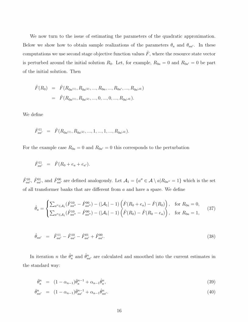
We use piecewise linear, convex functions to approximate value functions of spares at an
aggregated level. The usefulness of piecewise linear functions in VFAs was first documented
in Godfrey & Powell (2001) and Godfrey & Powell (2002). Figure 5 illustrates the VFA with
piecewise linear components. Note that the VFA contains both linear terms on the disaggre-
gate level (i.e. the bank level) and aggregate piecewise linear terms. The existence of aggregate
19
01 0( )gR x
01gV
01R
01δ
02 0( )gR x
02gV
02R
02δ
03R
03δ
04R
04δ
05R
05δ
Figure 5: VFA with nonlinear components. The arcs on the left represent the purchasingdecisions. The arcs in the middle are linear value function terms on the disaggregate level; onthe right are piecewise linear aggregate VFA terms for every group.
and disaggregate VFA components comes from the fact that under the aggregation paradigm
we look at the marginal value of a spare transformer, va, as containing two components. We
can write for a ∈ Ak: va = vgk + δa. One value component, vg
k, is derived from the group level
and the other, δa, is a correction term that differentiates spares in a group. Of course, none
of these values is known, so we set out to describe how they can be estimated.
We define
ykr = the flow on the rth segment of the piecewise linear function
of group k,
vgkr = estimate of the slope of the rth segment of the piecewise
linear function of group k,
δa = slope of the disaggregate VFA term a.
The approximate problem is to find
minx0
∑a∈A
∑d∈Dbuy
c0adx0ad +∑a∈A
δaR0a +K∑
k=1
|Ak|−1∑r=0
vgkrykr
(47)
20

subject to:
∑a∈Ak
R0a −|Ak|−1∑
r=0
ykr = 0 ∀ k (48)
0 ≤ ykr ≤ 1 ∀ r,k (49)
x0 ∈ X ′0 (50)
where X ′0 is the feasible region defined by (11)-(13). Note that the double sum in (47) is the
aggregate VFA component V g0 (Rg
0) and that (48) ensures flow conservation in the aggregate
nodes.
The raw materials for the estimation of VFA slopes are the left and right sample gradients
as defined in equations (21) and (22). The right gradient can be calculated if Rn0a is 0, the left
gradient if Rn0a is 1. We define the sample gradient on the group level as:
vg,right,nk = min
a∈A,Rn0a=0
vright,na (51)
vg,left,nk = min
a∈A,Rn0a=1
vleft,na . (52)
The aggregate gradients are the minimum of the left and right gradients in the group. We
find that using the minimum function to aggregate sample gradients produces much better
solutions than using simple averages. Now we can calculate the sample correction terms δna as
the difference between the disaggregate sample gradient and the aggregate sample gradient:
δna =
vright,n
a − vg,right,nk , if a ∈ Ak and Rn
0a = 0
vleft,na − vg,left,n
k , if a ∈ Ak and Rn0a = 1.
(53)
It remains to be shown how to use vg,right,nk , vg,left,n
k , and δna to update their respective VFA
terms. The update of δn−1a follows the usual scheme
δna = (1− αn−1)δn−1
a + αn−1δna . (54)
Updating the piecewise linear VFA components V g0k(Rg
0k) requires a more involved proce-
dure. Godfrey & Powell (2001), Topaloglu & Powell (2003), and Powell et al. (2004) propose
21

different methods. Common to all methods is a preliminary step where vg,left,nk is used to
update the slope to the left of Rgn0k and vg,right,n
k is used to update the slope to the right of
Rgn0k . The formula for this preliminary step is
unkr =
(1− αn−1)vg,n−1
kr + αn−1vg,right,nk if r = Rgn
0k ,
(1− αn−1)vg,n−1kr + αn−1v
g,left,nk if r = Rgn
0k − 1,
vg,n−1kr otherwise.
(55)
Now we would be done except that the updated estimate might not be convex and a
procedure to restore convexity is needed. We follow the SPAR algorithm of Powell et al. (2004)
for concave functions and apply it to our convex case. This method restores convexity by
projecting the updated estimate of the slopes onto the space of monotone increasing functions.
The projection operation is an optimization problem of the form
minvgn
k
‖ vgnk − u
nk ‖2 (56)
subject to:
vgnk,r+1 − v
gnkr ≥ 0 (57)
which is easily solved since it involves simply averaging slopes around Rgn0k .
0 321
, 11g nkv
−
, 10g nkv
−
, 12g nkv
−
, 13g nkv
−
r0 321
r 0gnkR
0 321
1 2,gn gnk kv v
0gnkv
3gnkv
r 0gnkR
1nku
0nku2nku
3nku
Figure 6: Illustration of SPAR with a convexity violation to the left of Rgn0k = 3. The original
VFA is on the left, the intermediate update in the middle, and the result of the projection onthe right. The functions represent the slopes of the piecewise linear VFA term of group k.
22

Step 0 Initialize V 00 and set n = 1.
Step 1 Solve (47)-(50). If n = N + 1 stop. xN+10 is the solution.
Step 2a Sample W1(ωn) and determine gradients:
vright,n = (vright,na )a∈A,Rn
0a=0
vleft,n = (vleft,na )a∈A,Rn
0a=1
as defined in (21) and (22)
Step 2b Determine:
vg,right,n = (vg,right,nk )k=1,2,..,K,Rgn
0k <|Ak|
vg,left,n = (vg,left,nk )k=1,2,...,K,Rgn
0k >0
δn = (δna )a∈A
as defined in (51), (52), and (53) respectively.
Step 3a For every k = 1, 2, ...,K calculate vector unk = (un
kr)r<|Ak| as in (55).
Step 3b For every k project unk onto the space of monotone functions to get vgn
k = (vgnkr )r<|Ak| using (56)-(57).
Step 3c Calculate δn = (δna )a∈A as in (54).
Set n = n+ 1 and go to Step 1.
Figure 7: ADP algorithm for the spare allocation problem with aggregation.
Figure 6 shows the steps of the SPAR algorithm for a convexity violation to the left
of Rgn0k = 3. Figure 7 shows the steps of the ADP algorithm with piecewise linear VFA
components and aggregation.
5 Experimental Design
This section describes the setup of the numerical experiments that we perform to evaluate
the presented ADP algorithms and to analyze the PJM system. We are interested in the
solution quality produced by four different value function approximations. We study the
linear approximation of section 4.1 (abbreviated LINEAR), the quadratic approximation of
section 4.2 (QUAD) and the piecewise linear approximation of section 4.3 with two different
aggregations. We choose to aggregate by transmission owner (PLTO) and by location (PLLO).
These are the two most natural aggregations and they differ in a key point. The aggregation
by transmission owner requires a mechanism to allocate spares within each group. When
23
aggregating by location the allocation within a group is not important because transfer costs
to and from all the banks in a location are identical.
5.1 The p-Median Problem as Reference Solution
How to measure solution quality is a subtle and interesting point in this research. There is
a classic deterministic discrete location problem - the p-median problem - that serves very
well as a standard to compare against. In fact, with some restrictions our problem reduces
to a generalized p-median problem. Since p-median problems of the size encountered in this
research can be easily solved using commercial optimization software we are able to find
the optimal solution for these simplified problem instances. In these cases the goal for our
algorithms is to come close to optimal. In the cases where a problem instance violates p-
median assumptions we would expect to outperform the reference solution in some systematic
way or at least in most cases.
We refer the reader to Mirchandani (1990) and Labbe et al. (1995) for a detailed presen-
tation of the p-median problem. It aims to optimally locate p facilities among a discrete set
of possible locations. The facilities are used to satisfy demand in a discrete set of demand
locations. The objective is to minimize the total sum of transportation costs between facilities
and demand locations. At first sight the p-median problem looks very similar to the spare
transformer problem. A closer look reveals the differences.
The facilities in the p-median problem are assumed to have infinite capacity and therefore
demand is always satisfied and it is always satisfied from the “closest” facility (i.e. the one
with the lowest transportation costs).
This is clearly not the case in our problem. If there is a failure and the closest spare is
otherwise in use our model attempts to get the next closest spare. If there are more failures
than spares then failures are left unmet. If there is a spare available to meet a failure but
the transfer is not economical the failure is also left unmet. These are the three most obvious
differences to the p-median problem.
We can convert our problem to a p-median problem by assuming there is at most one
24

failure and the congestion costs at a failure location always outweigh the transfer costs of a
spare to that location. Making these assumptions puts us in the position to obtain optimal
solutions for interesting instances of our problem.
5.2 Test Data Sets
Table 1 describes all the data sets used in the experiments. The data sets are meant to
comprise an interesting mix of data characteristics. Data sets with the prefix MU include all
71 of PJM’s transformer banks in 42 substation locations. That means there are locations with
multiple banks. Data sets with the prefix SI include 42 banks in 42 locations. All locations
have a single bank.
Data sets MU1, MU2, SI1, SI2, and SI3 are used for testing the solution quality. The
others are used in the study of section 6.3. Among the five data sets used for testing MU1,
SI1 and SI2 assume a single transformer failure and our model is in this case equivalent to
the corresponding p-median problem. Data sets MU2 and SI3 allow for multiple independent
failures and we would expect to outperform the reference solutions in these cases. In all
five data sets we use hazard rate functions estimated by PJM (Chen & Egan (2006)) to
determine transformer failure probabilities. The failure probability of a transformer depends
on its age and its maintenance status which can be “good”, “average”, or “watch”. We obtain
bank failure probabilities from individual transformer failure probabilities by calculating the
probability of the event that “at least one transformer in the bank fails” over the period of
one year.
For the experiments, the inventory holding cost is 0. We also assume a single transformer
manufacturer and a fixed transformer purchase price of $5 million. This leaves the parameter
c1ad for d ∈ Dmove to be considered. The corresponding decision x1ad for d ∈ Dmove implies that
a spare is moved to a failure site and used to cover a failure. Thus, the cost parameter for that
decision is the transfer cost minus the one-year congestion cost. The former is incurred due
to the movement of the spare. The latter represents the benefit of avoided system congestion.
25

NameNo.
BanksNo.Loc.
SharedSpares
FailureGener.
Exp.No.
Failures
Transp.Cost
(millions)
TransferTime
(years)
Cong.Cost
Model
Cong.Cost(107)
min: 0.16MU1* 71 42 Yes Single 1 n.a. med: 0.26 n.a. med: 22.24
max: 0.43min: 0.01 Uniform
MU2 71 42 Yes Indep. 5.2 n.a. med: 0.24 between 12 med: 24.49max: 0.63 and 32
min: 0.23 min: 0.16MU3 71 42 Yes Indep. 2.7 med: 1.69 med: 0.26 n.a. med: 22.24
max: 3.45 max: 0.43min: 0.23 min: 0.16
MU4 71 42 No Indep. 2.7 med: 1.03 med: 0.26 n.a. med: 22.24max: 2.15 max: 0.43min: 0.23 min: 0.16
MU5 71 42 Yes Indep. 4.1 med: 1.69 med: 0.26 n.a. med: 33.36max: 3.45 max: 0.43min: 0.23 min: 0.09
MU6 71 42 Yes Indep. 2.7 med: 1.69 med: 0.19 n.a. med: 22.24max: 3.45 max: 0.36
min: 0.01SI1* 42 42 Yes Single 1 n.a. med: 0.37 n.a. med: 22.1
max: 0.98min: 0.25
SI2* 42 42 Yes Single 1 n.a. med: 0.25 n.a. med: 22.1max: 0.25min: 0.01 Uniform
SI3 42 42 Yes Indep. 2.6 n.a. med: 0.24 between 12 med: 23.76max: 0.63 and 32
Table 1: Data sets used for solution quality assessment.* Equivalent to the corresponding p-median problem.
We use two different scenarios for the congestion cost. One scenario consists of congestion
costs provided by PJM. In these cases we do not need a congestion cost model (denoted by n.a.
in Table 1). Of course we wish to show that our methods work for more than one congestion
cost scenario. The second scenario uses randomly generated congestion costs. The median
congestion cost of the two scenarios are very close. But otherwise the two scenarios are very
different. The real data has high variance and is skewed with a number of outliers that have
very high congestion cost. The randomly generated data - coming from a uniform distribution
- is much smoother.
The transfer cost contains two components, a) a transportation cost which is the cost to
effect the physical movement of the spare and b) a congestion cost component that accounts
for the system congestion while the spare is being transferred. The transfer time represents
26

the time it takes to organize and execute the spare movement. During the transfer time the
failure that initiated the spare movement is left unmet. If the transfer time is, for example,
three months then the transfer cost would include one quarter of the one-year congestion cost
at the destination location.
In reality little more than anecdotal evidence on actual transfer times is available. This is
why we need a model to generate artificial transfer times. We use different models. Sometimes
transfer times are multiples of the distance between locations, sometimes they are fixed, and
sometimes they have a fixed component and a linear variable component in the distance.
The location of the spares becomes more important as the variability in the transfer times
increases. Thus the purely variable case makes for good test cases for our algorithms.
The data sets that are used for the solution quality assessment are set up such that a
failure is always met with a spare if a spare is available. In this case the avoided congestion
cost is constant for a given sample realization and number of spares. It is therefore legiti-
mate to remove the avoided congestion costs from the objective function when evaluating two
competing solutions. By evaluating only the transfer cost we can get a sharper picture of the
relative solution quality than by looking at the entire objective function that includes large
constant avoided congestion cost terms.
5.3 Algorithm Tuning
ADP algorithms would not work well without parameters that ensure a good learning behavior.
The step sizes, αn−1, and the number of training iterations, N , are the most important
parameters.
Figure 8 shows how the average solution quality changes with the number of training
iterations for different problem instances using the PLLO algorithm. To obtain the graph we
ran the algorithm for each instance and periodically evaluated the solution of the approximate
problem. The evaluation of a solution is performed in slightly different ways. If the sample
space is easily enumerable (as in our single failure experiments) then the evaluation uses
all the scenarios and their probabilities to calculate the expectation of the relevant second
27

0 500 1000 1500 2000 2500 30000.85
0.9
0.95
1
1.05
1.1
1.15
1.2
iterations
cost
rat
io
Influence of Training Period on Solution Quality
SI3 - 12 SparesSI3 - 4 SparesSI1 - 8 SparesMU2 - 12 SparesMU2 - 8 SparesMU2 - 4 Spares
Figure 8: Average solution quality as a function of the number of training iterations fordifferent problem instances using the PLLO algorithm. Each line is an average of 5 differentsample paths where each sample path (ω1, ω2, ..., ω3000) contains one sample for each iteration.The expected transfer cost is evaluated in increments of 50 iterations and divided by theexpected transfer cost of the corresponding p-median solution to obtain the cost ratio.
stage costs. If the sample space is not enumerable we use 3000 randomly drawn, and equally
weighted failure scenarios to approximate the expectation. The graphs in figure 8 show the
cost ratio which is the quality of the PLLO solution divided by the quality of the corresponding
p-median solution.
We see that the convergence behavior varies considerably across instances. For data set
SI3 with four spares (SI3 - 4 Spares), for example, the solution quality improves and stabilizes
within about 500 iterations. SI1 - 8 Spares on the other hand has much slower improvement
and the solution quality also varies considerably until around iteration 2700. Given the vari-
ation in convergence behavior it is appropriate to customize the number of training iterations
to each problem instance. In order to do so we run PLLO for each problem instance for
multiples of 500 iterations and pick N for which the average solution quality is best. Tables
3 in section 6.1 and 5 in section 6.2 show the results of this analysis.
28

0 200 400 600 800 1000 1200 1400 1600 1800 2000-1.07
-1.065
-1.06
-1.055
-1.05
-1.045
-1.04
-1.035
-1.03
-1.025
-1.02x 10
4
iterations
exp.
obj
ectiv
e fu
nctio
n va
lue
PLLO and QUAD Convergence Behavior
PLLOQUAD
Figure 9: An example of the convergence behavior of QUAD and PLLO (data set MU3, 10spares).
Run time considerations prevent us from using more than 600 iterations for QUAD which
is adequate according to our empirical tests.
Since convergence is key in ADP algorithms we have chosen the step size rules with great
care based on extensive experimental testing. For QUAD we use the quickly decreasing step
sizes αn−1 = 1n
and for LINEAR, PLTO, and PLLO we choose αn−1 = 54+n
which produces
step sizes that decline more slowly.
As figure 8 suggests ADP algorithms do not continuously improve over the training period.
For PLLO this characteristic is manageable and obtaining a very good solution is typical. This
is not the case for QUAD. Figure 9 shows by example that PLLO converges more uniformly
than QUAD. In the example QUAD finds a reasonable solution right around iteration 600
but does not systematically converge to it. This issue needs to be addressed in order to
ensure satisfactory solution quality. We employ the simplest possible fix: QUAD periodically
evaluates the solution of the approximate problem and remembers the best solution over the
course of the algorithm.
29

QUAD can suffer from excessive run times if the first stage MIP happens to be a difficult
problem instance. To address this we cannot rely on MIP warm starts as they are not nearly
as effective as LP warm starts. Instead we set a time limit of 17 seconds for the first stage
MIP. Every 50 iterations we increase the limit to 60 seconds for one iteration to increase the
chances of getting an optimal solution. Fortunately, the run time limit on the first stage MIP
does not appear to lead to a deterioration of the solution quality.
6 Numerical Results
This section presents the results of three different types of experiments. In section 6.1 we
carefully study the solution quality of different VFAs for data sets where the p-median solution
is optimal (MU1, SI1, SI2). The goal is to show that our algorithms provide consistently
near-optimal solutions. Section 6.2 contains results for more realistic data sets where the p-
median solution is not necessarily optimal (MU2, SI3). We wish to show that our algorithms
outperforms the reference solution when it is not optimal. Section 6.3 investigates spare
transformer allocation issues of practical interest using data sets MU3 - MU6.
6.1 Solution Quality when the Optimal Solution Is Known
Table 2 shows the experimental results for problem instances where p-median is optimal. We
ran each algorithm for each data set varying the number of transformer spares. The solutions
are evaluated as described in section 5.3. r is the cost ratio which is defined as
r =expected transfer cost of ADP solution
expected transfer cost of p-median solution.
N gives the number of training iterations and s the average run time in seconds. The entries
in the r and s columns are averages over five different sample paths (ω1, ω2, ..., ωN).
LINEAR works very well in cases with one bank per location. Its bad performance for
cases with multiple banks reflects the bunching issue analyzed in section 4.1. PLTO does
address the bunching problem to a degree but shows sometimes poor performance when the
number of spares is large.
30

LINEAR PLTO QUAD PLLODataSet
No.Spares r N s r N s r N s r N s
MU1 1 1.00 500 271 1.00 500 168 1.00 100 1041 1.00 500 1684 1.30 2000 646 1.05 2000 632 1.02 400 4195 1.00 1500 4868 1.76 2000 645 1.15 2000 634 1.04 400 4473 1.00 2000 651
SI1 1 1.00 500 42 1.00 500 41 1.00 100 166 1.00 500 424 1.02 2000 161 1.07 2000 158 1.08 600 1121 1.02 1000 828 1.04 2000 159 1.42 2000 159 1.14 600 2055 1.01 3000 242
SI2 1 1.01 500 40 1.01 500 158 1.01 100 161 1.01 500 414 1.01 2000 161 1.04 2000 158 1.01 400 654 1.00 1500 1218 1.02 2000 160 1.16 2000 158 1.02 400 651 1.00 3000 241
Table 2: Solution quality and computational effort for instances where p-median is optimal.r is the ratio of the transfer cost of the ADP solution to the transfer cost of the p-mediansolution, N is the number of iterations, and s is the elapsed time in seconds. r and s areaverages with sample size 5. Runs are measured on a single processor (Intel P4), 3.06 GHzmachine.
QUAD on the other hand produces generally good solutions even though the run times
for the larger instances (MU1) are fairly high. PLLO provides excellent solutions and shows
good run-time behavior. The cost ratio is always within 2% of the optimal and the largest
instance solves in less than 11minutes.
Iterations Run TimeDataSet
No.Spares 500 1000 1500 2000 2500 3000 s/500it
MU1 1 1.00 1.00 1.00 1.00 1.00 1.00 1664 1.03 1.01 1.00 1.00 1.00 1.01 1648 1.06 1.04 1.03 1.00 1.01 1.01 161
SI1 1 1.00 1.00 1.00 1.00 1.00 1.00 414 1.04 1.02 1.03 1.02 1.02 1.02 408 1.09 1.06 1.03 1.04 1.04 1.01 40
SI2 1 1.01 1.01 1.01 1.01 1.01 1.01 404 1.02 1.02 1.00 1.01 1.00 1.01 408 1.07 1.04 1.02 1.02 1.02 1.00 40
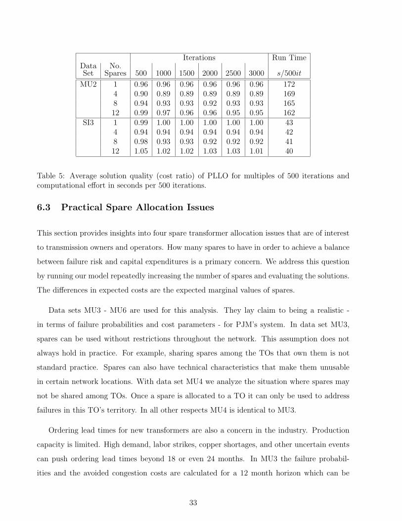
Table 3: Average solution quality (cost ratio) of PLLO for multiples of 500 iterations andcomputational effort in seconds per 500 iterations.
Table 3 quantifies the trade off between run time and solution quality for PLLO. We also
use these results to pick the best number of training iterations for PLLO as described in
31

section 5.3. This table shows the run times per 500 iterations. Technically, this is an average
run time but for each problem instance the run times per 500 iterations is nearly constant. We
see that 500 iterations are always enough to bring the solution quality within 10 percentage
points of the best achievable value. The rest of the iterations is spent closing this gap.
6.2 Solution Quality when the Optimal Solution Is Unknown
Table 4 shows the experimental results for problem instances where p-median is not necessarily
optimal.
LINEAR PLTO QUAD PLLODataSet
No.Spares r N s r N s r N s r N s
MU2 1 0.96 500 173 0.96 500 171 0.96 100 1283 0.96 500 2034 0.91 2000 686 0.90 2000 669 0.89 400 13322 0.89 1000 3718 1.11 2000 661 0.94 2000 663 0.98 400 12690 0.93 2000 68812 1.50 2000 664 1.10 2000 653 1.04 600 19571 0.96 2500 854
SI3 1 1.00 500 43 1.00 500 42 1.00 100 287 0.99 500 604 0.94 2000 167 0.98 2000 161 0.99 400 1872 0.94 500 608 0.92 2000 168 1.11 2000 161 1.01 400 1781 0.92 2000 17912 1.03 2000 164 1.51 2000 160 1.10 400 2699 1.01 3000 260
Table 4: Solution quality and computational effort for instances where p-median is not optimal.r is the cost ratio, N is the number of iterations, and s is the elapsed time in seconds. r ands are averages with sample size 5.
This table documents the problem with QUAD which are the excessive run times for most
runs with data set MU2. PLLO is again the best algorithm, outperforming the p-median
solution almost always and by as much as 11%. PLLO solves instance SI3 - 12 Spares in
less than 5 minutes and MU2 - 12 Spares in less than 15 minutes which indicates that the
algorithm could also handle problems with more locations.
Table 5 shows the results of the convergence analysis. We see that 500 iterations are
enough to bring the solution quality within 4 percentage points of the best achievable value.
32
Iterations Run TimeDataSet
No.Spares 500 1000 1500 2000 2500 3000 s/500it
MU2 1 0.96 0.96 0.96 0.96 0.96 0.96 1724 0.90 0.89 0.89 0.89 0.89 0.89 1698 0.94 0.93 0.93 0.92 0.93 0.93 16512 0.99 0.97 0.96 0.96 0.95 0.95 162
SI3 1 0.99 1.00 1.00 1.00 1.00 1.00 434 0.94 0.94 0.94 0.94 0.94 0.94 428 0.98 0.93 0.93 0.92 0.92 0.92 4112 1.05 1.02 1.02 1.03 1.03 1.01 40
Table 5: Average solution quality (cost ratio) of PLLO for multiples of 500 iterations andcomputational effort in seconds per 500 iterations.
6.3 Practical Spare Allocation Issues
This section provides insights into four spare transformer allocation issues that are of interest
to transmission owners and operators. How many spares to have in order to achieve a balance
between failure risk and capital expenditures is a primary concern. We address this question
by running our model repeatedly increasing the number of spares and evaluating the solutions.
The differences in expected costs are the expected marginal values of spares.
Data sets MU3 - MU6 are used for this analysis. They lay claim to being a realistic -
in terms of failure probabilities and cost parameters - for PJM’s system. In data set MU3,
spares can be used without restrictions throughout the network. This assumption does not
always hold in practice. For example, sharing spares among the TOs that own them is not
standard practice. Spares can also have technical characteristics that make them unusable
in certain network locations. With data set MU4 we analyze the situation where spares may
not be shared among TOs. Once a spare is allocated to a TO it can only be used to address
failures in this TO’s territory. In all other respects MU4 is identical to MU3.
Ordering lead times for new transformers are also a concern in the industry. Production
capacity is limited. High demand, labor strikes, copper shortages, and other uncertain events
can push ordering lead times beyond 18 or even 24 months. In MU3 the failure probabil-
ities and the avoided congestion costs are calculated for a 12 month horizon which can be
33

Expected Marginal Values of Transformer Spares
0
0.5
1
1.5
2
2.5
3
3.5
4
4.5
1 2 3 4 5 6 7 8 9 10 11 12 13 14 15 16 17 18 19 20 21 22 23 24
Number of Spares
$ m
illio
nMU3 MU4 MU5 MU6
Figure 10: Expected marginal values of transformer spares as a function of the number ofspares. Each data point is an average over five sample paths (ω1, ω1, ..., ωN) where N = 2000.
interpreted as a 12 month ordering lead time. MU5 uses an 18 month horizon instead.
Finally, it is of interest to explore the effect of switchable spares. Any spare can be pre-
prepared for service at the substation where it is stored. Turning on such a switchable spare
is a matter of a few days. If a spare is not switchable positioning within the substation and
putting it in service can take up to one month. Data set MU3 assumes switchable spares that
take 5 days to put into service. MU6 assumes non-switchable spares which require 30 days
of preparation. It is important to stress that this distinction is only relevant for substations
with an on-site spare.
Figure 10 shows the results of the marginal value analysis. In order to determine the
optimal number of spares one looks for the point where the marginal value hits the marginal
cost of a spare. The cost of a spare has to be prorated to match the one year time horizon of
the model.
As would be expected, the sharing of spares (MU3 vs. MU4) has a strong impact on the
34

optimal number. Assuming a marginal cost of $1 million the optimal number is 8 with sharing
and between 14 and 15 without. If the marginal cost is $500, 000 the numbers are 14 and
18 respectively. The relative effect of transformer sharing decreases as the marginal cost go
down.
Comparing MU3 with MU5 we see that the effect of the ordering lead time on the optimal
number is relatively small and also shrinks as the marginal cost decreases. If the marginal
cost is $1 million/$1.5 million for MU3/MU5 the optimal number is 8 for MU3 and between
9 and 10 for MU5. If the marginal cost is $500, 000/$750, 000 then the optimal number is
approximately 14 for MU3 and 15 for MU5.
The curve for MU3 dominates the curve for MU6. That means that if spares are switchable
the optimal number increases. The intuitive interpretation of this behavior is that with
switchable spares it is very desirable to have an on-site spare as opposed to bringing in an off-
site spare. With additional spares the model can potentially grab more of the on-site/off-site
transfer cost difference. Since this difference is big if spares are switchable it can justify more
spares.
7 Conclusions and Further Research
In this paper we have introduced a two-stage spare transformer allocation model. Current
technology is far from being able to solve large realistic instances of this problem exactly. We
use an ADP approach to solve the model approximately and observe that VFAs are needed that
can take into account the non-separable behavior of the true value function. We introduce
two such VFAs and test the obtainable solution quality. PLLO is the best algorithm. It
consistently produces very good solutions and solves very efficiently. We show that the model
can be used to answer spare transformer allocation questions of practical interest.
A useful extension of this research is the introduction of multi-period models that reflect
the true dynamic nature of high-voltage transformer management. They could be used to
model the transformer population and the electric grid as they change over time and answer
questions about the timing of transformer purchases and replacements, spare deployment
35

policies, and many others. The performance characteristics of the algorithm used in this
paper are so good that it would be a suitable algorithmic starting point for the richer and
larger multi-period transformer management models.
36
References
Bertsekas, D. & Tsitsiklis, J. (1996), Neuro-Dynamic Programming, Athena Scientific, Bel-mont, MA. 2
Birge, J. & Louveaux, F. (1997), Introduction to Stochastic Programming, Springer-Verlag,New York. 2
Chen, Q. M. & Egan, D. M. (2006), ‘A bayesian method for transformer life estimation usingperks’ hazard function’, IEEE Transactions on Power Systems 21(4), 1954–1965. 25
Chowdhury, A. A. & Koval, D. O. (2005), ‘Development of probabilistic models for com-puting optimal distribution substation spare transformers’, IEEE Transactions on IndustryApplications 41(6), 1493–1498. 3
Godfrey, G. & Powell, W. B. (2002), ‘An adaptive, dynamic programming algorithm forstochastic resource allocation problems I: Single period travel times’, Transportation Science36(1), 21–39. 3, 19
Godfrey, G. A. & Powell, W. B. (2001), ‘An adaptive, distribution-free approximation for thenewsvendor problem with censored demands, with applications to inventory and distributionproblems’, Management Science 47(8), 1101–1112. 19, 21
Helmberg, C. (2000), Semidefinite programming for combinatorial optimization, Technicalreport, Konrad-Zuse-Zentrum fuer Informationstechnik Berlin, Berlin. 15
Kall, P. & Wallace, S. (1994), Stochastic Programming, John Wiley & Sons, New York. 2
Kogan, V. I., Roeger, C. J. & Tipton, D. E. (1996), ‘Substation distribution transformersfailures and spares’, IEEE Transactions on Power Systems 11(4), 1905–1912. 3
Labbe, M., Peeters, D. & Thisse, J.-F. (1995), Location on networks, in M. Ball, T. L.Magnanti, C. L. Monma & G. L. Nemhauser, eds, ‘Handbooks in Operations research andManagement Science: Network Routing’, Elsevier, Amsterdam. 3, 24
Laporte, G., Louveaux, F. V. & van Hamme, L. (1994), ‘Excact solution to a location problemwith stochastic demands’, Transportation Science 28(2), 95–103. 2, 7
Li, W., Vaahedi, E. & Mansour, Y. (1999), ‘Determining number and timing of substationspare transformers using a probabilistic cost analysis approach’, IEEE Transactions onPower Delivery 14(3), 934–939. 3
Louveaux, F. V. & Peeters, D. (1992), ‘A dual-based procedure for stochastic facility location’,Operations Research 40(3), 564–573. 2, 7
Mirchandani, P. B. (1990), The p-median problem and generalizations, in P. B. Mirchandani& R. L. Francis, eds, ‘Discrete Location Theory’, Wiley, New York. 3, 24
Ntaimo, L. & Sen, S. (2005), ‘The million-variable ”march” for stochastic combinatorial opti-mization’, Journal of Global Optimization 32, 385–400. 2, 3, 7
Powell, W. B. (2007), Approximate Dynamic Programming: Solving the curses of dimension-ality, John Wiley and Sons, New York. 8
37

Powell, W. B. & Topaloglu, H. (2004), Fleet management, in S. Wallace & W. Ziemba, eds,‘Applications of Stochastic Programming’, Math Programming Society - SIAM Series inOptimization, Philadelphia. 3
Powell, W. B. & Van Roy, B. (2004), Approximate dynamic programming for high dimensionalresource allocation problems, in J. Si, A. G. Barto, W. B. Powell & D. W. II, eds, ‘Handbookof Learning and Approximate Dynamic Programming’, IEEE Press, New York. 8
Powell, W. B., George, A., Bouzaiene-Ayari, B. & Simao, H. (2005), Approximate dynamicprogramming for high dimensional resource allocation problems, in ‘Proceedings of theIJCNN’, IEEE Press, New York. 2
Powell, W. B., Ruszczynski, A. & Topaloglu, H. (2004), ‘Learning algorithms for separableapproximations of stochastic optimization problems’, Mathematics of Operations Research29(4), 814–836. 3, 21, 22
Powell, W. B., Shapiro, J. A. & Simao, H. P. (2002), ‘An adaptive dynamic program-ming algorithm for the heterogeneous resource allocation problem’, Transportation Science36(2), 231–249. 8, 11
Puterman, M. L. (1994), Markov Decision Processes, John Wiley & Sons, New York. 8
Sen, S. (2005), Algorithms for stochastic mixed-integer programming models, in K. Aardal,G. L. Nemhauser & R. Weismantel, eds, ‘Handbooks in Operations Research and Manage-ment Science: Discrete Optimization’, North Holland, Amsterdam. 2
Topaloglu, H. (2001), Dynamic programming approximations for dynamic programming prob-lems, Ph.d. dissertation, Department of Operations Research and Financial Engineering,Princeton University. 3
Topaloglu, H. & Powell, W. B. (2003), ‘An algorithm for approximating piecewise linearconcave functions from sample gradients’, Operations Research Letters 31(1), 66–76. 21
Topaloglu, H. & Powell, W. B. (2006), ‘Dynamic programming approximations for stochas-tic, time-staged integer multicommodity flow problems’, Informs Journal on Computing18(1), 31–42. 2, 3, 8
38