An Integrated Decomposition and Approximate Dynamic

1

An Integrated Decomposition and ApproximateDynamic Programming Approach for On-demand

Ride PoolingXian Yu* and Siqian Shen*

Abstract—Through smartphone apps, drivers and passengerscan dynamically enter and leave ride-hailing platforms. Asa result, ride-pooling is challenging due to complex systemdynamics and different objectives of multiple stakeholders. In thispaper, we study ride-pooling with no more than two passengergroups who can share rides in the same vehicle. We dynamicallymatch available drivers to randomly arriving passengers and alsodecide pick-up and drop-off routes. The goal is to minimize aweighted sum of passengers’ waiting time and trip delay time. Aspatial-and-temporal decomposition heuristic is applied and eachsubproblem is solved using Approximate Dynamic Programming(ADP), for which we show properties of the approximated valuefunction at each stage. Our model is benchmarked with the onethat optimizes vehicle dispatch without ride-pooling and the onethat matches current drivers and passengers without demandforecasting. Using test instances generated based on the New YorkCity taxi data during one peak hour, we conduct computationalstudies and sensitivity analysis to show (i) empirical convergenceof ADP, (ii) benefit of ride-pooling, and (iii) value of futuresupply-demand information.

Index Terms—Mobility on Demand (MoD), supply-demanduncertainty, ride-pooling, spatial-temporal decomposition, ap-proximate dynamic programming

I. INTRODUCTION

Increasing population and environmental issues have ledto various shared-mobility forms, including carsharing andride-hailing services whose demand drastically increased inthe past decade (see [1]). Ref. [2] thoroughly reviewed theliterature related to ride-hailing including vehicle dispatching,scheduling, routing, and solution methods mainly based onoptimization and heuristics. In this paper, we study an on-demand ride-pooling problem over a finite time horizon, andthe decisions include matching drivers with passengers, as wellas finding optimal routes for drivers to pick up and drop offmatched passengers. We focus on the case where no morethan two groups of passengers may share rides at the sametime in one vehicle, and prove value function properties ofthe dynamic problem characterized by an ADP approach.

To show the benefit and feasibility of pooling rides in prac-tice, [3] considered the minimum fleet problem and conductedlarge-scale simulation to show that by pooling rides, the taxifleet size in the Manhattan area of the New York City canbe reduced by 40% without delaying existing trips. Ref. [4]studied ride-pooling effects under different pricing schemes

*Xian Yu and Siqian Shen are with Department of Industrial and Op-erations Engineering at the University of Michigan in Ann Arbor, [email protected], [email protected]

and demonstrated the importance of pooling rides for revenuemaximization. Reported in [5], UberPOOL has saved $4.5million worth in fuel costs in India since launch. Large-scaleoperations of ride-pooling were considered in [6]–[10] withthe deployment of simulation, parallel computing, machinelearning, stochastic control, and combinatorial optimizationtechniques. Their studies demonstrated the possibility and ef-fectiveness of implementing on-demand ride-sharing at scale.

In this paper, we model the ride pooling problem as a mul-tistage stochastic program and incorporate different objectivesof individual passenger groups and drivers, measured basedon waiting time and trip delay. If directly using dynamicprogramming, the number of states will grow exponentiallyas the number of drivers and passengers grows, resultingin the “curse of dimensionality” issue. We employ ADP[11] for the tractability of modeling system dynamics. Whiledynamic programming calculates value functions exactly, ADPexploits an approximation of the value function at each stage[12]. Furthermore, by examining spatial-temporal structuresof supply-demand data, we propose a heuristic decompositionscheme and only apply ADP to each subproblem to achievebetter computational performance. Our goal is to show theconvergence of ADP, benefit of pooling rides, and value ofsupply-demand information via testing real-world instancesusing different parameters.

A. Literature Review

Ride-hailing operations are closely related to several fun-damental mathematical problems including matching, vehiclerouting, service scheduling, and queueing networks. Differentfrom the traditional static settings in these problems wheredemands and supplies are pre-given, the drivers (supply) andpassengers (demand) randomly arrive in on-demand ride-hailing systems, urging the use of stochastic and dynamicmethods to ensure solution quality. Ref. [13] deployed arolling horizon approach and matched drivers with randompassenger arrivals in each horizon without optimizing detailedroutes. Refs. [14] and [15] considered algorithms for onlinematching and the latter specifically focused on the ride-sharingapplication. Ref. [16] utilized queueing networks to developa continuous linear program that accounted for the time-varying property of arrival rates of passengers and drivers indifferent locations. In addition to matching and routing, pricingand vehicle rebalancing are two other important issues thatcan significantly affect operational efficiency and ride-hailing

2

revenue, and they were studied in [16]–[22] and in [23]–[28],respectively.

Incorporating ride-pooling into ride-sharing can increasemodeling and computational complexity, but its benefit hasbeen justified in the previously mentioned work, such as [3]–[5]. The study of pooling rides among deterministic sets ofdrivers and passengers dates back to [29], who used spatial-temporal networks for pooling taxi rides. Ref. [30] appliedheuristics to develop routing strategies in taxi-pooling. Ref.[31] assumed that all the trips are known in advance, andintroduced a “shareability” network and a graph-based modelto quantify the benefits of ride pooling.

In practice, mobility-on-demand (MoD) or autonomousmobility-on-demand (AMoD) systems ubiquitously involveinformation uncertainty. Refs. [8], [10], [23], [26], [28] em-ployed queueing theories, machine learning, and/or stochas-tic control to predictively position vehicles under randomspatial-temporal distributions of demand and supply. Ref. [32]proposed a dynamic request-vehicle assignment heuristic anda rebalancing policy for AMoD systems, and evaluated thevalue of demand information through simulation. On the otherhand, the design and operations of MoD/AMoD systems needto account for diverse objectives of drivers, passengers andsystem operators, whose benefits may be conflicting. Ref. [31]optimized ride-pooling by considering the maximum numberof trips that can be shared and the maximum delay customerscan tolerate. Ref. [33] characterized quality of service in ride-sharing through potential trip delay probability. They proposeda predictive positioning method to improve quality of service.Under demand uncertainties, [27], [34] proposed data-drivendistributionally robust optimization schemes to ensure servicefairness.

The difficulty of involving uncertainty in MoD- or AMoD-related system optimization including ride-pooling optimiza-tion, is to design scalable solution approaches. When consid-ering vehicle routing in ride-pooling, the problem is closelyrelated to the Vehicle Routing Problem (VRP) [35], Dial-a-Ride [36] and Pickup and Delivery problems [37], [38],which are NP-hard in general. To implement on-demand ride-pooling strategies, [6], [7], [9], [10], [39] avoided explicitlymodeling road networks and routing decisions, and deployedsimulation, local search, reinforcement learning, parallel com-puting to handle real-world large-scale data. Specifically, [40]aimed to dynamically assign passenger requests and exploitedhybrid simulated annealing to obtain quick solutions. Ref. [7]presented a heuristic approach for real-time high-capacity ride-hailing that dynamically produced routes given randomly ar-riving demand requests and uncertain vehicle distribution. Ref.[6] proposed a real-time online simulation and parallelizationframework to study taxi ride-pooling at scale. Refs. [41] and[42] developed a taxi-sharing system to handle passengers’real-time requests.

B. Purposes of the Paper

This paper models dynamic ride-pooling as a multistagestochastic program and uses ADP ( [11], [43]) for solvingthe problem through a heuristic decomposition scheme. Refs.

[44]–[46] are representative literature of applying ADP forsolving stochastic VRP and other transportation problems. Weincorporate multiple objectives including minimizing the totalpassengers’ waiting time, trips’ delay time, and unsatisfied triprequests, to improve quality of service. Note that although thedrivers’ profit is not specified in the objective function, thepassenger-oriented objective can potentially increase drivers’profit when more passengers’ requests are satisfied. In thenumerical studies, a reward formula is built to calculate andreflect drivers’ benefits based on the results of passengers’reward. Moreover, this paper only focuses on how to dynami-cally match and route drivers and passengers while assuminggiven fixed prices.

The main objective is to study the structure of valuefunctions in ADP. Specifically, we explore the linkage betweenvalue functions in different states and prove the monotonicityresult. We also heuristically decompose time horizon andservice region into sub-periods and sub-regions to allow moreefficient implementation. We conduct numerical studies oninstances generated from real-world data, and consider twobenchmark approaches: (i) myopic, which solves a determin-istic linear program in each stage and implements the solutionsin a rolling horizon way and (ii) NotPool, which does not allowride pooling.

C. Structure of the Paper

The remaining of this paper is organized as follows. InSection II, problem settings and a deterministic formulationare introduced. In Section III, we develop the ADP algorithmfor on-demand ride-pooling with no more than two passengergroups in any shared ride. In Section IV, a spatial-temporaldecomposition heuristic is described for implementing ADP.In Section V, we test a diverse set of instances and presentcomputational results. We conclude the paper and state futureresearch directions in Section VI.

II. PROBLEM DESCRIPTION AND FORMULATIONS

A. Assumptions and Notation

The paper has the following assumptions: (i) the capacityof each vehicle is fixed and pre-given (which we set as 4 seatsexcluding the driver seat in our later computational studies);(ii) every vehicle can be shared by at most two passengergroups; (iii) at the end of each time stage, passengers withno matches quit the system. Assumptions (i) and (iii) can bejustified by practical implementation and customer behavior,respectively. Assumption (ii) is a limitation and it is mainlymade for modeling simplicity. In practice, UberPool and LyftLine Apps can allow more than two passenger groups to sharerides at the same time. When the number of ride-sharinggroups increases from 2 to 3, combinations of pickup anddrop-off sequences increase drastically, while the trip delaytime and customer waiting time can be longer. On the otherhand, pooling more rides can potentially increase revenue andwe will explore the more general case without Assumption (ii)in our future research.

3

In our problem, for every driver, an attribute vector acorresponds to a state such that:

a = (oa,La, Na),

where oa denotes the current location of the driver, La is anordered list containing all the places that the driver will visit,and Na is the number of passengers that are currently assignedto the driver. Note that |La| is 0 at minimum (when a vehicleis empty) and 3 at maximum (when a vehicle is occupiedby a passenger group and needs to pick up another passengergroup). Let Ait be the set of all possible driver attribute vectorsa, whose |La| = i in stage t, for i = 0, 1, 2, 3. We denoteAt = A0

t ∪ A1t ∪ A2

t ∪ A3t for each stage t ∈ {1, . . . , T}.

For every passenger request, an attribute vector b alsocorresponds to a state following:

b = (ob,db, Nb),

where ob denotes the origin of passenger(s), db denotes thedestination of passenger(s), and Nb denotes the number ofpassengers in the request. Let Bt be the set of all possiblepassenger attribute vectors b in stage t, Rta be the number ofdrivers with attribute vector a in stage t, and Rt = (Rta)a∈At

be the resource state vector in stage t. Similarly, let Dtb bethe number of passengers with attribute b in stage t, and Dt =(Dtb)b∈Bt be the demand state vector in stage t.

Define variable xtab as the number of drivers with attribute aassigned to passengers with attribute b in stage t, and variablexta∅ as the number of drivers with attribute a not assigned toany passengers in stage t. Let d ∈ D represent a decision indexreferring to either assigning a driver to pick up a particulargroup of passengers or instructing that driver to wait at thecurrent position, i.e., D = Bt ∪ {∅}. Note that there maybe other actions such as vehicle rebalancing and empty-carrerouting, which are not considered in this paper. Variablext = (xtad)a∈At,d∈D denotes the overall decision vector instage t.

B. Objective Function

Our objective function accounts for passengers’ waitingtime and trip delay time, described in detail as follows.

1) Passengers’ Waiting time: Passengers’ waiting time ismeasured using the distance that the assigned driver movesfrom his/her current location to the passengers’ origin. Forevery pair of driver with attribute a = (oa,La, Na) andpassenger group with attribute b = (ob,db, Nb), the waitingtime is:

wab =‖ oa − ob ‖, (1)

where oa,ob denote the driver’s and passenger’s current loca-tions, respectively. The norm ‖ · ‖ measures the travel distance(or time) from oa to ob.

2) Passengers’ Delay time: Passengers’ delay time wouldonly occur when they start to share rides with other passengers.The distance of detour is used to measure the delay time (i.e.,the difference between the original individual travel time andthe total travel time if they share rides). For each pair ofpassenger groups to be dropped off by the same driver, wedenote the driver’s current location by o1, the first group of

passengers’ destination by d1, the second group of passengers’origin and destination by o2 and d2, respectively. Whichpassenger group to drop off first is decided based on respectiveshortest paths. Specifically, when ‖ d2 − o2 ‖≤‖ d1 − o2 ‖,the driver will first drop off the second group of passengers.In this case, only the first group of passengers is delayed, andthe delay time is

dab =‖ o2− o1 ‖ + ‖ d2− o2 ‖ + ‖ d1− d2 ‖ − ‖ d1− o1 ‖ .(2)

When ‖ d2 − o2 ‖>‖ d1 − o2 ‖, the driver will first dropoff the first group of passengers. In this case, the total delaytime of both groups of passengers is

dab = ‖ o2 − o1 ‖ + ‖ d1 − o2 ‖ − ‖ d1 − o1 ‖+ ‖ d1 − o2 ‖ + ‖ d1 − d2 ‖ − ‖ d2 − o2 ‖ . (3)

The above prepossessing procedures are detailed in Algo-rithm 1.

Algorithm 1 Preprocessing1: For each pair of driver a = (oa,La, Na) and passenger b = (ob,db, Nb)2: Use Google map API to calculate travel time and waiting time wab following Eq.

(1).3: if ‖ d2 − o2 ‖≤‖ d1 − o2 ‖ then4: Calculate delay time dab following Eq. (2);5: else6: Calculate delay time dab following Eq. (3).7: end if

C. Current-stage-based Deterministic Formulation

In each stage t, using current drivers and passengers, onecan solve the following linear program to myopically matchdrivers with passenger groups and determine pick-up and drop-off routes, where set S = {(a, b) ∈ At × Bt | Na +Nb ≤ c1}is defined as the set of all possible driver-passenger assign-ments constrained by vehicle capacities.

min λ1∑

a∈A0t∪A1

t(a,b)∈S

xtabwab + λ2∑

a∈A1t

(a,b)∈S

xtabdab +M∑

a6∈A0t∪A1

tb∈Bt

xtab

+N∑

a∈A0t∪A1

t(a,b)6∈S

xtab + P∑b∈Bt

Dtb −∑

a∈A0t∪A1

t

xtab

(4)

s.t.∑d∈Bt

xtab + xta∅ = Rta, ∀a ∈ At (5)

∑a∈At

xtab ≤ Dtb, ∀b ∈ Bt (6)

xtad ≥ 0, ∀a ∈ At, d ∈ D. (7)

In the objective function (4), the first two terms are a weightedsum of passengers’ total waiting time and trip delay timewhere λ1 + λ2 = 1, λ1, λ2 ≥ 0, and the last three termsdenote the penalty costs associated with assigning unavailabledrivers, exceeding vehicle capacities, and unsatisfied passen-gers’ demand, respectively. Constraint (5) is flow conservationfor drivers, i.e., the total number of drivers is capacitated.Constraint (6) is flow conservation for passengers, i.e., thenumber of drivers assigned to passengers with certain attributeis no more than the total number of passengers with that

4

attribute. Since the constraint matrix composed by (5) and (6)is totally unimodular, integral solutions can be attained at allextreme points of the above linear program (4)–(7) (see [47]).Therefore, constraint (7) only requires that all the decisionvariables are non-negative, yielding a linear program to solvefor each stage t, given updated Rta and Dtb at the beginningof the stage.

III. APPROXIMATE DYNAMIC PROGRAMMING

The traditional dynamic programming algorithm approxi-mates value functions around pre-decision states, and thereforeit requires the calculation of expectation over future informa-tion. We propose an ADP variant (see [12]) to approximatevalue functions around post-decision states.

A. Dynamic Process

Denote the state of the system in stage t as St = (Rt, Dt),called the pre-decision state, meaning that St is measured be-fore making a decision in stage t. The exogenous informationis denoted as Wt = Dtb, where Dtb is the number of newpassengers with attribute b known between stages t− 1 and t.The dynamic process in which the system evolves is

(S0,x0, Sx0 ,W1, S1,x1, S

x1 ,W2, S2, . . . , St,xt, S

xt , . . . , ST ).

Here Sxt represents the state after taking decision xt, knownas the post-decision state (see [12]). Denote Sxt = (Rxt , D

xt )

where Rxt = (Rxta)a∈At,x and Dxt = (Dx

tb)b∈Bt , which rep-resent the “post-decision” values of Rt and Dt, respectively.Next, we describe how to construct post-decision states ofresource Rxt and demand Dx

t .1) Post-decision State: For each pre-decision state St =

(Rt, Dt), define a transition function aM that acts decision xton the attribute vector a ∈ At and let a′ = aM (a,xt), ∀a ∈At. Define set At,x with a′ = (o′a,L′a, N ′a) ∈ At,x.

In each stage t, consider all pairs (a, b) ∈ At × Btthat have xtab > 0. Recall that b = (ob,db, Nb), and seto′a = oa, L′a = La ∪ {ob,db}, N ′a = Na + Nb. If |L′a| = 3,the route is determined using the shortest-path strategy inSection II-B2, and the driver is not available until the currenttrip is completed. To better represent post-decision states,consider an indicator function:

δa(a,xt) =

{1, if aM (a,xt) = a

0, otherwise.

Then, the post-decision resource state Rxt = (Rxta)a∈At,xis

updated using

Rxta′ =∑a∈At

∑d∈D

δa′(a,xt)xtad, ∀a′ ∈ At,x. (8)

The post-decision demand state Dxt = (Dx

tb)b∈Bt,xis updated

usingDxtb = Dtb −

∑a∈At

xtab, ∀b ∈ Bt. (9)

The state transition function SM,x follows SM,x(St,xt) =Sxt = (Rxt , D

xt ) where the post-decision resource and demand

state Rxt , Dxt follow (8) and (9), respectively.

2) Pre-decision State: For a post-decision state Sxt =(Rxt , D

xt ), we gather the exogenous information Wt+1 from

stages t to t+ 1. To determine the pre-decision state St+1 =(Rt+1, Dt+1), define a transition function aM,W that cap-tures the physical movement of vehicles with attribute a =(oa,La, Na) from t to t + 1. That is, a′ = aM,W (a), ∀a ∈At,x, where a′ = (o′a,L′a, N ′a) ∈ At+1.

When La is nonempty, let l1 be the first element in La (i.e.,the first location that driver is going to visit). After findingthe shortest path from oa to l1, let o′a be where the driverarrives if he/she moves one stage from oa to l1 followingthe shortest path. Let L′a = La − {l1} if o′a = l1. Also, letN ′a = Na − Nb if the driver drops off a passenger groupwith attribute b = (ob,db, Nb). Similarly, consider an indicatorfunction:

δa(a) =

{1, if aM,W (a) = a

0, otherwise.

Then the pre-decision resource state Rt+1 = (Rt+1,a)a∈At+1

is updated using

Rt+1,a′ =∑

a∈At,x

δa′(a)Rxta, ∀a′ ∈ At+1. (10)

Because unsatisfied demand is immediately lost in every stage(i.e., Assumption (iii)), the pre-decision demand state Dt+1 =(Dt+1,b)b∈Bt+1 can be updated as

Dt+1,b = Wt+1, ∀b ∈ Bt+1. (11)

The state transition function SM,W is SM,W (Sxt ,Wt+1) =St+1 = (Rt+1, Dt+1), where the pre-decision resource anddemand state Rt+1, Dt+1 follow (10) and (11), respectively.

B. Dynamic Programming Equation

The objective function in problem (4)–(7) is denoted byCt(St,xt). Then the Bellman equation is conventionally givenby:

Vt(St) = minxt∈Xt

{Ct(St,xt) + γE[Vt+1(St+1)|St]} ,(12)

where γ is the discount factor, E[Vt+1(St+1)|St] denotes theconditional expectation of objective value at time t+ 1 giventhe current state St, and the feasible region Xt consists ofconstraints (5)–(7).

Using the post-decision state, Eq. (12) can be decomposedinto two steps:

Vt(St) = minxt∈Xt

{Ct(St,xt) + γV xt (Sxt )} , (13)

V xt (Sxt ) = E[Vt+1(St+1)|Sxt ]. (14)

Next, we configure an approximation function Vt(Sxt ) for

value function V xt (Sxt ) around post-decision state Sxt , whichyields the following optimization problem:

Ft(St) = minxt∈Xt

{Ct(St,xt) + γVt(S

xt )}. (15)

The basic algorithmic strategy is as follows: At iteration n, asample path ωn is randomly chosen, and then the following

5

optimization problem for every time stage t = 0, 1, . . . , T issolved under the current approximation:

Ft(Snt ) = min

xt∈Xt

{Ct(S

nt ,xt) + γV n−1

t (SM,x(Snt ,xt))}.

(16)After obtaining the optimal solution xnt , compute the post-decision state Sx,nt = SM,x(Snt ,xt) and the next pre-decisionstate Snt+1 = SM,W (Sx,nt ,Wt(ω

n)). Then, solve the optimiza-tion problem (16) again to continue the process from stage tto stage t+1 until reaching stage T . After that, advance to thenext iteration n+ 1. The algorithm is terminated if it reachesa given maximum number of iterations (denoted by N ) andalso the objective function becomes stable.

To efficiently computing (16), consider an approximationfunction that is linear in Rta, given by:

Vtn−1

(Sxt ) = Vtn−1

(Rxt ) =∑a′

vta′Rxta′

=∑a′

vta′∑a

∑d

δa′(a,xt)xtad

=∑a

∑d

vn−1t,aM (a,xt)

xtad.

Then the optimization problem (16) becomes

Ft(Snt ) = min

xt∈Xt

{Ct(S

nt ,xt) + γ

∑a

∑d

vn−1t,aM (a,xt)

xtad

}.

(17)What is left now is how to update the coefficient vn−1

ta in thelinear approximation function. Note that vn−1

ta is the slope ofFt(S

nt ) with respect to Rxta, which can be computed using:

vnt−1,a =∂F (St)

∂Rxt−1,a

=∑a′∈At

∂F (St)

∂Rta′

∂Rta′

∂Rxt−1,a

,

where ∂F (St)/∂Rta′ are the dual variables associated withconstraints (5) in model (17), denoted by νnta′ . We have

∂Rta′

∂Rxt−1,a

=

{1, if a′ = aM,W (axt−1)

0, otherwise.

This means that if from stage t− 1 to stage t, attribute axt−1

evolves to a′ = aM,W (axt−1), then we only need to optimizeover variable νnta′ , and update vnt−1,a′ = νnta′ . After obtainingvnt−1,a′ , the coefficient can be updated using

vnt−1,at−1= (1− αn−1)vn−1

t−1,at−1+ αn−1v

nt−1,a′ , (18)

where αn−1 is a stepsize in iteration n. The above steps ofADP are summarized in Algorithm 2.

C. Value Function Properties

Suppose that the state space is equipped with a partial order�, then a value function is monotone if it satisfies

St � S′t ⇒ Vt(St) ≤ Vt(S′t), ∀t ≤ T. (19)

A common example of � is the generalized component-wiseinequality. In the ADP approach, our state can be decomposedinto St = (Rt, Dt). For any two states St = (Rt, Dt), S

′t =

Algorithm 2 ADP1: Initialize value functions V 0

t , t = 0, 1, . . . , T and state S10 . Set n = 1.

2: while n < N do3: Randomly pick a sample path ωn.4: for t = 0, 1, . . . , T do5: Gather all drivers’ state At and passengers’ requests Bt. For each pair

of a ∈ At and b ∈ Bt, implement Algorithm 1 to obtain parameterswab, dab.

6: Solve the optimization problem (16). Let xnt be the optimal solution, and

νta′ be the dual associated with the resource constraint.7: Update the value function using (18).8: Update the state:

Sx,nt = SM,x(Sn

t ,xt), Snt+1 = SM,W (Sx,n

t ,Wt(ωn)).

9: end for10: n := n+ 111: end while

(R′t, D′t), we have

St � S′t ⇐⇒ Rt ≤ R′t, Dt = D′t. (20)

The monotonicity of the value function indicates that we havemore resource in stage t+ 1 if starting with more resource instage t, regardless of the outcome of the random informationWt+1.

Theorem 1. Let � be the generalized component-wise in-equality over all dimensions of the state space. The optimalvalue function is monotone based on (19) and (20).

The detailed proof of Theorem 1 is provided in the onlinee-companion.

We continue exploring quantitative properties of ADP valuefunctions. The linear program in each time t is:

min∑a∈Atd∈D

(ctad + γvnt,aM (a,d))xtad

s.t. (5)–(7),

where ctad is the cost related to each action xtad, andvnt,aM (a,d) is the approximate value function. (We abbreviatevnt,aM (a,d) as vnad in our later discussion.) Using specific costterms in the objective function (4), the dual of the above linearprogram is

max∑

a∈At

νaRta +∑b∈Bt

µbDtb (21)

s.t. νa + µb ≤ λ1wab − P + γvnab, ∀a ∈ A0t , (a, b) ∈ S (22)

νa + µb ≤ λ1wab + λ2dab − P + γvnab, ∀a ∈ A1t , (a, b) ∈ S

(23)

νa + µb ≤ N + γvnab, ∀a ∈ A0t ∪ A1

t , (a, b) 6∈ S (24)

νa + µb ≤M + γvnab, ∀a 6∈ A0t ∪ A1

t , b ∈ Bt (25)νa ≤ γvna∅, ∀a ∈ At (26)

µb ≤ 0, ∀b ∈ Bt, (27)

where νa is the Lagrangian multiplier (dual variable) associ-ated with constraint (5), and µb is the dual variable associatedwith constraint (6).

Based on strong duality and complementary slackness, thefollowing result reveals the relationship between dual variablesand value functions.

Lemma 1. 1) If a 6∈ A0t ∪ A1

t or a ∈ A0t ∪ A1

t , (a, b) 6∈S, ∀b ∈ Bt, then νa = γvna∅.

2) If a ∈ A0t , then

νa ≥ minb:(a,b)∈S {λ1wab − P + γvnab};

6

3) if a ∈ A1t , then

νa ≥ minb:(a,b)∈S {λ1wab + λ2dab − P + γvnab}.

Please refer to the online e-companion for the detailed proofof Lemma 1.

IV. TEMPORAL AND SPATIAL DECOMPOSITION

Two decomposition schemes based on time and location areproposed to improve the solution time of the ADP approach.

A. Temporal Decomposition

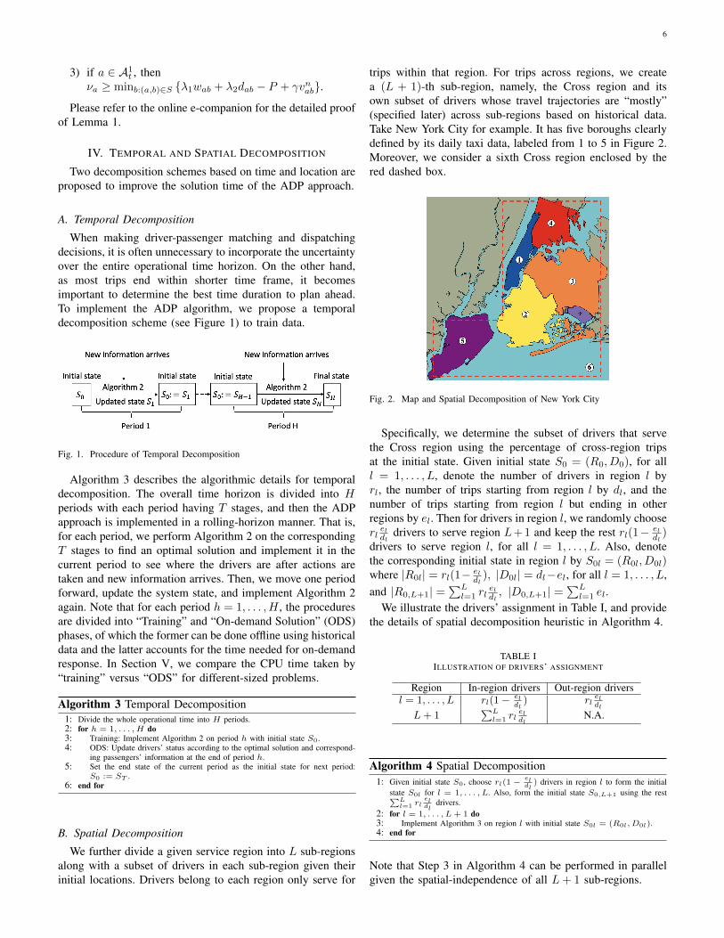
When making driver-passenger matching and dispatchingdecisions, it is often unnecessary to incorporate the uncertaintyover the entire operational time horizon. On the other hand,as most trips end within shorter time frame, it becomesimportant to determine the best time duration to plan ahead.To implement the ADP algorithm, we propose a temporaldecomposition scheme (see Figure 1) to train data.

Fig. 1. Procedure of Temporal Decomposition

Algorithm 3 describes the algorithmic details for temporaldecomposition. The overall time horizon is divided into Hperiods with each period having T stages, and then the ADPapproach is implemented in a rolling-horizon manner. That is,for each period, we perform Algorithm 2 on the correspondingT stages to find an optimal solution and implement it in thecurrent period to see where the drivers are after actions aretaken and new information arrives. Then, we move one periodforward, update the system state, and implement Algorithm 2again. Note that for each period h = 1, . . . ,H , the proceduresare divided into “Training” and “On-demand Solution” (ODS)phases, of which the former can be done offline using historicaldata and the latter accounts for the time needed for on-demandresponse. In Section V, we compare the CPU time taken by“training” versus “ODS” for different-sized problems.

Algorithm 3 Temporal Decomposition1: Divide the whole operational time into H periods.2: for h = 1, . . . , H do3: Training: Implement Algorithm 2 on period h with initial state S0.4: ODS: Update drivers’ status according to the optimal solution and correspond-

ing passengers’ information at the end of period h.5: Set the end state of the current period as the initial state for next period:

S0 := ST .6: end for

B. Spatial Decomposition

We further divide a given service region into L sub-regionsalong with a subset of drivers in each sub-region given theirinitial locations. Drivers belong to each region only serve for

trips within that region. For trips across regions, we createa (L + 1)-th sub-region, namely, the Cross region and itsown subset of drivers whose travel trajectories are “mostly”(specified later) across sub-regions based on historical data.Take New York City for example. It has five boroughs clearlydefined by its daily taxi data, labeled from 1 to 5 in Figure 2.Moreover, we consider a sixth Cross region enclosed by thered dashed box.

Fig. 2. Map and Spatial Decomposition of New York City

Specifically, we determine the subset of drivers that servethe Cross region using the percentage of cross-region tripsat the initial state. Given initial state S0 = (R0, D0), for alll = 1, . . . , L, denote the number of drivers in region l byrl, the number of trips starting from region l by dl, and thenumber of trips starting from region l but ending in otherregions by el. Then for drivers in region l, we randomly chooserleldl

drivers to serve region L+ 1 and keep the rest rl(1− eldl

)drivers to serve region l, for all l = 1, . . . , L. Also, denotethe corresponding initial state in region l by S0l = (R0l, D0l)where |R0l| = rl(1− el

dl), |D0l| = dl−el, for all l = 1, . . . , L,

and |R0,L+1| =∑Ll=1 rl

eldl, |D0,L+1| =

∑Ll=1 el.

We illustrate the drivers’ assignment in Table I, and providethe details of spatial decomposition heuristic in Algorithm 4.

TABLE IILLUSTRATION OF DRIVERS’ ASSIGNMENT

Region In-region drivers Out-region driversl = 1, . . . , L rl(1− el

dl) rl

eldl

L+ 1∑L

l=1 rleldl

N.A.

Algorithm 4 Spatial Decomposition1: Given initial state S0, choose rl(1 −

eldl

) drivers in region l to form the initialstate S0l for l = 1, . . . , L. Also, form the initial state S0,L+1 using the rest∑L

l=1 rleldl

drivers.2: for l = 1, . . . , L+ 1 do3: Implement Algorithm 3 on region l with initial state S0l = (R0l, D0l).4: end for

Note that Step 3 in Algorithm 4 can be performed in parallelgiven the spatial-independence of all L+ 1 sub-regions.

7

V. NUMERICAL RESULTS

We first test randomly generated small instances to con-figure parameter for implementing ADP (see the online e-companion), and then use instances generated based on real-world data collected from New York City taxi daily operationsto perform numerical tests. We use the New York City data forone peak-hour operations (from 8am to 9am). Two benchmarkpolicies are described below.

• Benchmark 1 (B1): Solve the linear program (4)–(7) forthe current stage given information of existing drivers andpassengers. Repeat the process for each stage in a rollinghorizon way.

• Benchmark 2 (B2): Apply decomposition-based ADPwithout ride-pooling.

A. Experimental Setup

According to the parameter configuration results, we setM = 1000, N = 1000, P = 500, weight λ = (0.2, 0.8), andstepsize αn = 1/n in each iteration n of the ADP algorithm.Our test instances are based on data from the New York CityTaxi and Limousine Commission (TLC) (see [48]). The taxitrip records include pick-up and drop-off dates/times, loca-tions, trip distances, itemized fares, rate types, payment types,and driver-reported passenger counts. There are 265 differentlocations among all five boroughs (i.e., Manhattan, Bronx,Brooklyn, Queens and Staten). In Table II, we summarizethe total number of trips in one month within each borough(see Row ‘In’), going out of each borough (see Row ‘Out’),and their approximate ratios. Note that the number of tripswithin Cross region is the sum of out-region trips in all thefive boroughs. Staten has much fewer trips compared to other

TABLE IITRIPS DISTRIBUTION AMONG BOROUGHS

Manhattan Bronx Brooklyn Queens Staten CrossIn 301618 30833 296324 271349 123 162155

Out 35639 9747 84577 32158 34 N.A.Ratio 1 0.1 1 1 N.A. 0.5

boroughs, and thus we eliminate this borough in our tests. Theratio of trips among all remaining five sub-regions is roughly1:0.1:1:1:0.5, which is used to generate their associated driversin the initial state.

We first test a finite horizon with each stage length being 5minutes. The data from 1/1/17 to 6/30/17 (181 days) duringthe rush hour 8am-9am, and is divided into 12 stages. Foreach stage and each location, we fit the historical data into thenegative binomial distribution, and then generate test instances.The average trip duration of all the data is 14.7 minutes witha standard deviation 1 minute and 42 seconds, and the averagenumber of trips per hour is 1523. Drivers’ profits are calculatedusing a base fee $2.5 plus $2 per mile similar to New YorkCity Taxi fares. Let |A| and |B| be the total number of driversand passengers in all five regions, respectively. We vary theirvalues to change instance sizes in our later analysis.

B. In-sample Tests and Results of Smaller Instances

First, we focus on time period 8:00am-8:25am and Manhat-tan borough with 69 nodes. Let T = 5, |A| = 10, 20. In TableIII, we display waiting time (WT) and delay time (DT) perpassenger per stage, profits per driver per stage and proportionof unsatisfied demand (UD) per stage.

TABLE IIICOMPARISON OF THE RESULTS OF ADP, B1, AND B2

|A| |B| Metrics ADP B1 B2

10 54

WT (min.) 4.33 4.11 4.29DT (min.) 1.54 1.28 0.00Profits ($) 9.72 9.67 4.34

UD (%) 18.77% 19.82% 33.25%

10 72


UD (%) 18.14% 19.46% 31.57%

20 56


UD (%) 0.68% 1.01% 6.62%

20 73


UD (%) 0.81% 1.27% 7.76%

In Table III, when the number of drivers increases from10 to 20, the proportion of unsatisfied demand for ADP dropsfrom above 18% to below 1%, showing much better quality ofservice. Comparing ADP, B1 and B2, we observe that ADPalways yields the lowest unsatisfied demand rate, while B2always has the highest rate. However, ADP may result inlonger waiting time than B1 because the drivers pick up morepassengers. Although B2 always has zero delay time (since itdoes not allow for pooling), it performs badly in waiting time,drivers’ profits and unsatisfied demand. When we increase |B|while keeping |A| unchanged, almost all the above results inTable III increase slightly.

In summary, having more drivers can lead to better perfor-mance in waiting time, delay time and proportion of unsatisfieddemand, although profits per driver could become slightly less.

C. Results of Larger Instances

We then test the decomposition-based ADP for all five sub-regions of New York City for 1-hour ride-pooling operations.Let T = 4, H = 3 (and thus 12 stages in total with each stagebeing 5 minutes). In Table IV, the results in each region areaggregated by a weighted sum where the weight is the ratioof drivers in each region.

We focus on the case where |A| = 108, |B| = 393 anduse bar charts to illustrate the overall performance in TableIV as well as the performance in each region separately. InFigure 3, x-axis denotes different approaches. From TableIV, when the driver-passenger ratio is approximately 1:4, theproportion of unsatisfied demand is around 6%, producedby ADP, whereas it drops to below 0.3% when the driver-passenger ratio becomes 1:2. This result can provide guidelinesfor ridesharing operators to control driver-passenger balance

8

TABLE IVRESULTS OF ADP, B1, B2 WHEN T = 4, H = 3 FOR ONE-HOUR TAXI

OPERATIONS IN NEW YORK CITY

|A| |B| Metrics ADP B1 B2

108 286


UD (%) 0.28% 0.34% 2.40%

108 393


UD (%) 6.05% 6.17% 11.92%

180 283


UD (%) 0.00% 0.00% 0.02%

180 389


UD (%) 0.15% 0.16% 0.40%

with desired quality-of-service levels. From Figure 3, in all fiveregions, ADP yields the lowest unsatisfied demand rate, whereB2 always gains the longest waiting time and the highestunsatisfied demand. On the other hand, across different re-gions, Brooklyn has the best results with the lowest unsatisfieddemand rate and shortest delay time, while Cross region yieldsthe longest waiting and delay time because the related tripsusually have longer travel distances.

D. Value of Uncertainty

Now consider Manhattan borough and uncertain demandover twelve time stages with each stage being 5-minute long(i.e., 60 minutes). We first solve the problem containing thefirst six stages (i.e., 30 minutes), update the state of the system,and solve the problem for the later six stages. Alternatively,we repeatedly solve the problem for every four/three/twostages (i.e., 20/15/10 minutes) to further reduce the problemdimension and the number of stages we “look ahead.” We use|A| = 30, |B| = 120 and present the results of T = 6, T =4, T = 3, T = 2 in Table V. The cases with T = 4 andT = 3 perform relatively better overall. Both cases with T = 6and T = 2 have worse unsatisfied demand, and the latteris much worse than the other three in all three approaches.However, T = 2 has slightly better waiting time, trip delaytime, and profit. These results agree on that it may not benecessary to take into account the information 20 minutesfrom now since the average trip duration is 14.7 minutes withstandard deviation being roughly 1 minute. However, if thedispatcher only forecasts one or two stages’ future demand,the unsatisfied demand rate is intolerably high, indicating theimportance of looking-ahead, stochastic policies.

We further test the model with each stage being one minuteto examine result sensitivity dependent on the granularity ofdata. We consider demand during 8am to 8:30am (i.e., 30stages) and look ahead 5-minute demand uncertainty each

(a) Overall (b) Manhattan

(c) Bronx (d) Brooklyn

(e) Queens (f) Cross

Fig. 3. Performance overall and in different regions

TABLE VVALUE OF UNCERTAINTY RESULTS BY VARYING T AND H

T H Metrics ADP B1 B2

6 2

WT (min.) 3.94 3.54 4.47DT (min.) 0.77 0.62 0.00Profits ($) 7.49 7.34 4.10UD (%) 2.90% 2.71% 15.67%

4 3


3 4


2 6


time, resulting in parameter setting T = 6, H = 5. Wecompare the solutions with the ones in the previous casehaving each stage being five minutes and use parameter settingT = 2, H = 3 so that we also look ahead five minuteseach time. The corresponding results are displayed in TableVI. We observe that cases with 1-minute stage length haveshorter waiting and delay time, but they have much higher andunacceptable unsatisfied demand rates due to Assumption (i).

9

TABLE VIVALUE OF UNCERTAINTY RESULTS BY VARYING TIME UNIT

T H Metrics ADP B1 B2

6 5


2 3


E. Computational TimeWe end this section by showing the computational time for

different instances. First, in Table VII we report the CPU timefor solving instances having each stage being five minutes withT = 4, H = 3. As the decomposed ADP can be implementedfor each region in parallel, we record the maximum timeused by each of the five regions. Moreover, the training timefor each period is recorded separately in Columns “h = 1”,“h = 2” and “h = 3”, and the on-demand solution time ispresented in Column ”ODS”. All the training steps can beperformed offline while the on-demand implementation justextracts the updated value functions to solve a linear programin each stage, which only takes no more than 90 seconds forthe largest instance and it is almost linearly dependent on thenumber of drivers and passengers. All times that exceed 3600-second CPU time limit are labeled by N.A.

TABLE VIITRAINING TIME AND ON-DEMAND SOLUTION (ODS) TIME (IN SECONDS)

|A| |B| h = 1 h = 2 h = 3 ODS

108285 83.62 83.85 82.03 12.26390 149.51 149.63 148.85 11.58498 354.58 351.82 350.93 24.56

180285 145.47 143.7 143.2 10.09390 402.18 400.9 403.48 22.14498 861.76 825.43 817.29 45.08

360285 517.86 519.14 518.78 82.21390 1354.97 1291.5 1290.5 90.01498 N.A. N.A. N.A. N.A.

Second, we compare the CPU time taken by the two settingsused in Section V-D. Specifically, when letting each stagebeing five minutes (with T = 2 and H = 3), on averagethe instances take 20.34 seconds, 18.28 seconds, and 22.37seconds for training data in periods h = 1, 2, 3, respectively,and the on-demand computation only requires 2.01 seconds.However, when each stage is one minute (with T = 6, H = 5),based on the same 30-minute data, the ADP approach takesaround 2400 seconds for training in each period, and the ODSphase requires 275.5 seconds. This also justifies our choice ofletting each stage being five minutes.

VI. CONCLUSIONS

We considered ride-pooling problem with no more than twopassenger groups sharing rides at the same time. We employed

the ADP approach to solve the problem dynamically and ex-ploited properties of value functions. A decomposition heuris-tic was developed to divide the whole space and operationtime into sub-regions and several periods. Numerical resultsshowed quick convergence and result stability of using ADP.We compared ADP with two benchmarks, and demonstratedthat it can serve the most passengers among all, showing theimportance of including future demand uncertainty into ride-pooling decision making. Also, ADP led to shorter waitingtime per passenger as compared to the benchmark with noride-pooling, showing the importance of pooling rides in ride-hailing systems.

For future research, we plan to investigate ride poolingproblems allowing more than two passenger groups in thesame vehicle. One can also incorporate pricing and vehiclerelocation into the current operational model, to investigatehow they affect ride pooling strategies.

ACKNOWLEDGMENT

We thank the Associate Editor and four anonymous review-ers for their detailed comments and constructive feedback. Theauthors are grateful for the support of the NSF grant CMMI-1727618.

REFERENCES

[1] S. Wallsten, “The competitive effects of the sharing economy: How isUber changing taxis,” Technology Policy Institute, vol. 22, 2015.

[2] N. Agatz, A. Erera, M. Savelsbergh, and X. Wang, “Optimization fordynamic ride-sharing: A review,” European Journal of OperationalResearch, vol. 223, no. 2, pp. 295–303, 2012.

[3] M. Vazifeh, P. Santi, G. Resta, S. Strogatz, and C. Ratti, “Addressingthe minimum fleet problem in on-demand urban mobility,” Nature, vol.557, no. 7706, p. 534, 2018.

[4] J. Jacob and R. Roet-Green, “Ride solo or pool: The impactof sharing on optimal pricing of ride-sharing services,”Available at SSRN: https://ssrn.com/abstract=3008136 orhttp://dx.doi.org/10.2139/ssrn.3008136, 2017.

[5] S. Agarwal, “Uberpool has saved $4.5 million worthin fuel import costs in india since launch,” https://economictimes.indiatimes.com/small-biz/startups/newsbuzz/uberpool-has-saved-4-5-million-worth-in-fuel-import-costs-in-india-since-launch/articleshow/64455325.cms, 2018.

[6] M. Ota, H. Vo, C. Silva, and J. Freire, “STaRS: Simulating taxi ridesharing at scale,” IEEE Transactions on Big Data, vol. 3, no. 3, pp.349–361, 2017.

[7] J. Alonso-Mora, S. Samaranayake, A. Wallar, E. Frazzoli, and D. Rus,“On-demand high-capacity ride-sharing via dynamic trip-vehicle assign-ment,” Proceedings of the National Academy of Sciences, vol. 114, no. 3,pp. 462–467, 2017.

[8] J. Alonso-Mora, A. Wallar, and D. Rus, “Predictive routing for au-tonomous mobility-on-demand systems with ride-sharing,” in 2017IEEE/RSJ International Conference on Intelligent Robots and Systems(IROS). IEEE, 2017, pp. 3583–3590.

[9] M. Zhu, X.-Y. Liu, and X. Wang, “An online ride-sharing path-planningstrategy for public vehicle systems,” IEEE Transactions on IntelligentTransportation Systems, vol. 20, no. 2, pp. 616–627, 2018.

[10] Z. Xu, Z. Li, Q. Guan, D. Zhang, Q. Li, J. Nan, C. Liu, W. Bian, andJ. Ye, “Large-scale order dispatch in on-demand ride-hailing platforms:A learning and planning approach,” in The 24th ACM SIGKDD Inter-national Conference on Knowledge Discovery & Data Mining. ACM,2018, pp. 905–913.

[11] D. P. Bertsekas, Dynamic programming and optimal control. AthenaScientific Belmont, MA, 1995, vol. 1, no. 2.

[12] W. B. Powell, Approximate Dynamic Programming: Solving the Cursesof Dimensionality. John Wiley & Sons, 2007, vol. 703.

[13] N. Agatz, A. L. Erera, M. W. Savelsbergh, and X. Wang, “Dynamicride-sharing: A simulation study in metro Atlanta,” Procedia-Social andBehavioral Sciences, vol. 17, pp. 532–550, 2011.

10

[14] M. Lowalekar, P. Varakantham, and P. Jaillet, “Online spatio-temporalmatching in stochastic and dynamic domains,” Artificial Intelligence,vol. 261, pp. 71–112, 2018.

[15] C. Dutta and C. Sholley, “Online matching in a ride-sharing platform,”arXiv preprint arXiv:1806.10327, 2018.

[16] E. Ozkan and A. R. Ward, “Dynamic matching for real-time rideshar-ing,” Available at SSRN: https://ssrn.com/abstract=2844451, 2016.

[17] S. Banerjee, D. Freund, and T. Lykouris, “Pricing and optimization inshared vehicle systems: An approximation framework,” arXiv preprintarXiv:1608.06819, 2016.

[18] L. Zha, Y. Yin, and Z. Xu, “Geometric matching and spatial pricingin ride-sourcing markets,” Transportation Research Part C: EmergingTechnologies, vol. 92, pp. 58–75, 2018.

[19] A. Fiat, Y. Mansour, and L. Shultz, “Flow equilibria via online surgepricing,” arXiv preprint arXiv:1804.09672, 2018.

[20] M. Chen, W. Shen, P. Tang, and S. Zuo, “Optimal vehicle dispatchingfor ride-sharing platforms via dynamic pricing,” in Companion of theThe Web Conference 2018. International World Wide Web ConferencesSteering Committee, 2018, pp. 51–52.

[21] V. Kamble, “On optimal pricing of services in on-demand labor plat-forms,” arXiv preprint arXiv:1803.06797, 2018.

[22] A. Gupta, B. Saha, and P. Banerjee, “Pricing decisions of car aggregationplatforms in sharing economy: A developing economy perspective,”Journal of Revenue and Pricing Management, pp. 1–15, 2018.

[23] R. Iglesias, F. Rossi, K. Wang, D. Hallac, J. Leskovec, and M. Pavone,“Data-driven model predictive control of autonomous mobility-on-demand systems,” in 2018 IEEE International Conference on Roboticsand Automation (ICRA). IEEE, 2018, pp. 1–7.

[24] K. Spieser, S. Samaranayake, W. Gruel, and E. Frazzoli, “Shared-vehiclemobility-on-demand systems: A fleet operator’s guide to rebalancingempty vehicles,” in Transportation Research Board 95th Annual Meet-ing, no. 16-5987. Transportation Research Board, 2016.

[25] H. R. Sayarshad and J. Y. Chow, “Non-myopic relocation of idlemobility-on-demand vehicles as a dynamic location-allocation-queueingproblem,” Transportation Research Part E: Logistics and TransportationReview, vol. 106, pp. 60–77, 2017.

[26] A. Braverman, J. G. Dai, X. Liu, and L. Ying, “Empty-car routing inridesharing systems,” arXiv preprint arXiv:1609.07219, 2016.

[27] F. Miao, S. Han, A. M. Hendawi, M. E. Khalefa, J. A. Stankovic,and G. J. Pappas, “Data-driven distributionally robust vehicle balancingusing dynamic region partitions,” in The 8th International Conferenceon Cyber-Physical Systems. ACM, 2017, pp. 261–271.

[28] R. Zhang and M. Pavone, “Control of robotic mobility-on-demandsystems: A queueing-theoretical perspective,” The International Journalof Robotics Research, vol. 35, no. 1-3, pp. 186–203, 2016.

[29] S. Yan, C.-Y. Chen, and C.-C. Wu, “Solution methods for the taxipooling problem,” Transportation, vol. 39, no. 3, pp. 723–748, 2012.

[30] X. Wei, “Routing for taxi-pooling problem based on ant colony opti-mization algorithm,” Revista de la Facultad de Ingenierıa, vol. 31, no. 7,2016.

[31] P. Santi, G. Resta, M. Szell, S. Sobolevsky, S. H. Strogatz, and C. Ratti,“Quantifying the benefits of vehicle pooling with shareability networks,”Proceedings of the National Academy of Sciences, vol. 111, no. 37, pp.13 290–13 294, 2014.

[32] J. Wen, N. Nassir, and J. Zhao, “Value of demand information in au-tonomous mobility-on-demand systems,” Transportation Research PartA: Policy and Practice, vol. 121, pp. 346–359, 2019.

[33] J. Miller and J. P. How, “Predictive positioning and quality of serviceridesharing for campus mobility on demand systems,” in 2017 IEEEInternational Conference on Robotics and Automation (ICRA). IEEE,2017, pp. 1402–1408.

[34] F. Miao, S. Han, S. Lin, Q. Wang, J. A. Stankovic, A. Hendawi,D. Zhang, T. He, and G. J. Pappas, “Data-driven robust taxi dispatchunder demand uncertainties,” IEEE Transactions on Control SystemsTechnology, vol. 27, no. 1, pp. 175–191, 2017.

[35] G. Laporte, “What you should know about the vehicle routing problem,”Naval Research Logistics, vol. 54, no. 8, pp. 811–819, 2007.

[36] J.-F. Cordeau and G. Laporte, “The dial-a-ride problem: Models andalgorithms,” Annals of Operations Research, vol. 153, no. 1, p. 29, 2007.

[37] M. W. Savelsbergh and M. Sol, “The general pickup and deliveryproblem,” Transportation Science, vol. 29, no. 1, pp. 17–29, 1995.

[38] G. Berbeglia, J.-F. Cordeau, and G. Laporte, “Dynamic pickup anddelivery problems,” European Journal of Operational Research, vol.202, no. 1, pp. 8–15, 2010.

[39] D. Bertsimas, P. Jaillet, and S. Martin, “Online vehicle routing: Theedge of optimization in large-scale applications,” Operations Research,vol. 67, no. 1, pp. 143–162, 2019.

[40] J. Jung, R. Jayakrishnan, and J. Y. Park, “Dynamic shared-taxi dispatchalgorithm with hybrid-simulated annealing,” Computer-Aided Civil andInfrastructure Engineering, vol. 31, no. 4, pp. 275–291, 2016.

[41] S. Ma, Y. Zheng, O. Wolfson et al., “Real-time city-scale taxi rideshar-ing.” IEEE Transactions on Knowledge and Data Engineering, vol. 27,no. 7, pp. 1782–1795, 2015.

[42] S. Ma, Y. Zheng, and O. Wolfson, “T-share: A large-scale dynamictaxi ridesharing service,” in Data Engineering (ICDE), 2013 IEEE 29thInternational Conference on. IEEE, 2013, pp. 410–421.

[43] D. P. Bertsekas and J. N. Tsitsiklis, “Neuro-dynamic programming: Anoverview,” in The 34th IEEE Conference on Decision and Control, vol. 1.IEEE, 1995, pp. 560–564.

[44] C. Novoa and R. Storer, “An approximate dynamic programmingapproach for the vehicle routing problem with stochastic demands,”European Journal of Operational Research, vol. 196, no. 2, pp. 509–515,2009.

[45] V. Schmid, “Solving the dynamic ambulance relocation and dispatchingproblem using approximate dynamic programming,” European Journalof Operational Research, vol. 219, no. 3, pp. 611–621, 2012.

[46] A. J. Kleywegt, V. S. Nori, and M. W. Savelsbergh, “Dynamic pro-gramming approximations for a stochastic inventory routing problem,”Transportation Science, vol. 38, no. 1, pp. 42–70, 2004.

[47] G. L. Nemhauser and L. A. Wolsey, Integer and Combinatorial Opti-mization. New York, NY: Wiley-Interscience, 1999.

[48] N. Taxi and L. Commission, “New York City’s taxi trip data,” http://www.nyc.gov/html/tlc/html/about/trip record data.shtml/, 2018, [On-line; accessed 19-March-2018].

Xian Yu Xian Yu received the B.S. degree from the Honors Science Programin Mathematics in Xi’an Jiaotong University, Xi’an, China, in 2017. She iscurrently a PhD candidate in the Department of Industrial and OperationsEngineering at the University of Michigan, Ann Arbor. Her research interestsinclude stochastic integer programming with applications in transportation andlogistics.

Siqian Shen Siqian Shen received the B.S. degree in Industrial Engineeringfrom Tsinghua University, China, in 2007, and the M.S. and Ph.D. degrees inIndustrial and Systems Engineering from the University of Florida, USA, in2009 and 2011, respectively. She is an Associate Professor in the Departmentof Industrial and Operations Engineering, University of Michigan at AnnArbor, and also an Associate Director for the Michigan Institute for Com-putational Discovery & Engineering (MICDE). Her research interests includestochastic programming, network optimization, and integer programming.Applications of her work include transportation and energy.

Documents

An Integrated Decomposition and Approximate Dynamic