APPROXIMATE DYNAMIC PROGRAMMING

LECTURE 2

LECTURE OUTLINE

• Review of discounted problem theory

• Review of shorthand notation

• Algorithms for discounted DP

• Value iteration

• Policy iteration

• Optimistic policy iteration

• Q-factors and Q-learning

• A more abstract view of DP

• Extensions of discounted DP

• Value and policy iteration

• Asynchronous algorithms

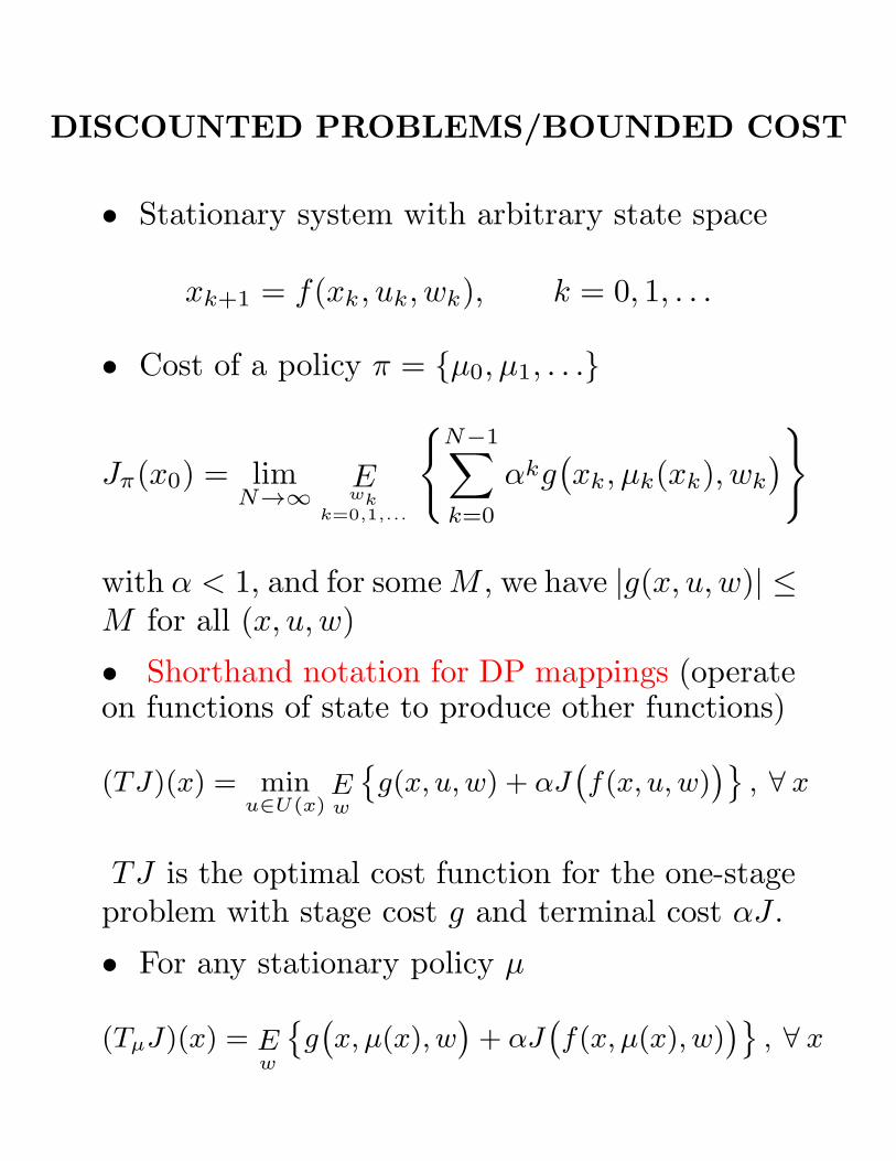
DISCOUNTED PROBLEMS/BOUNDED COST

• Stationary system with arbitrary state space

xk+1 = f(xk, uk, wk), k = 0, 1, . . .

• Cost of a policy π = {µ0, µ1, . . .}

Jπ(x0) = limN→∞

Ewk

k=0,1,...

{

N−1∑

k=0

αkg(

xk, µk(xk), wk

)

}

with α < 1, and for someM , we have |g(x, u, w)| ≤M for all (x, u, w)

• Shorthand notation for DP mappings (operateon functions of state to produce other functions)

(TJ)(x) = minu∈U(x)

Ew

{

g(x, u, w) + αJ(

f(x, u, w))}

, ∀ x

TJ is the optimal cost function for the one-stageproblem with stage cost g and terminal cost αJ .

• For any stationary policy µ

(TµJ)(x) = Ew

{

g(

x, µ(x), w)

+ αJ(

f(x, µ(x), w))}

, ∀ x

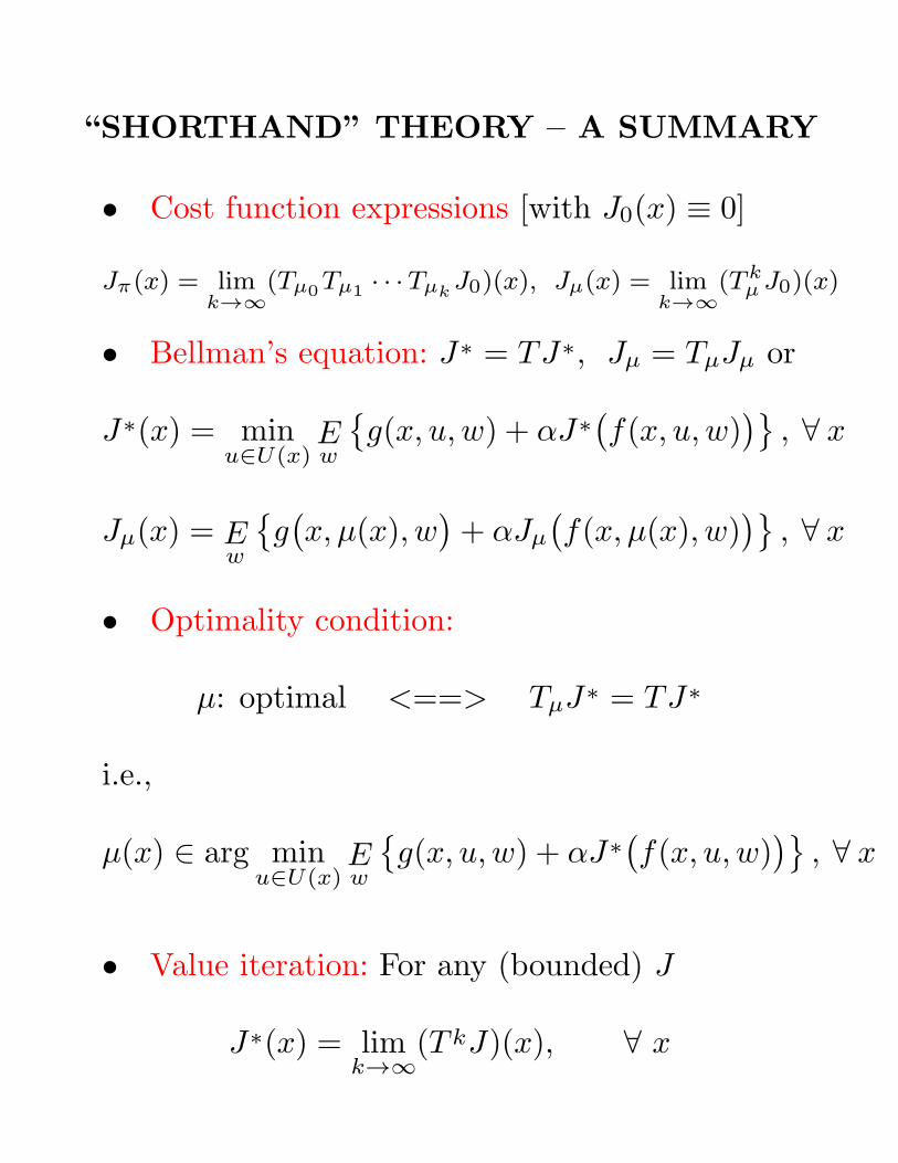
“SHORTHAND” THEORY – A SUMMARY

• Cost function expressions [with J0(x) ≡ 0]

Jπ(x) = limk→∞

(Tµ0Tµ1

· · ·TµkJ0)(x), Jµ(x) = lim

k→∞

(TkµJ0)(x)

• Bellman’s equation: J∗ = TJ∗, Jµ = TµJµ or

J∗(x) = minu∈U(x)

Ew

{

g(x, u, w) + αJ∗(

f(x, u, w))}

, ∀ x

Jµ(x) = Ew

{

g(

x, µ(x), w)

+ αJµ(

f(x, µ(x), w))}

, ∀ x

• Optimality condition:

µ: optimal <==> TµJ∗ = TJ∗

i.e.,

µ(x) ∈ arg minu∈U(x)

Ew

{

g(x, u, w) + αJ∗(

f(x, u, w))}

, ∀ x

• Value iteration: For any (bounded) J

J∗(x) = limk→∞

(T kJ)(x), ∀ x

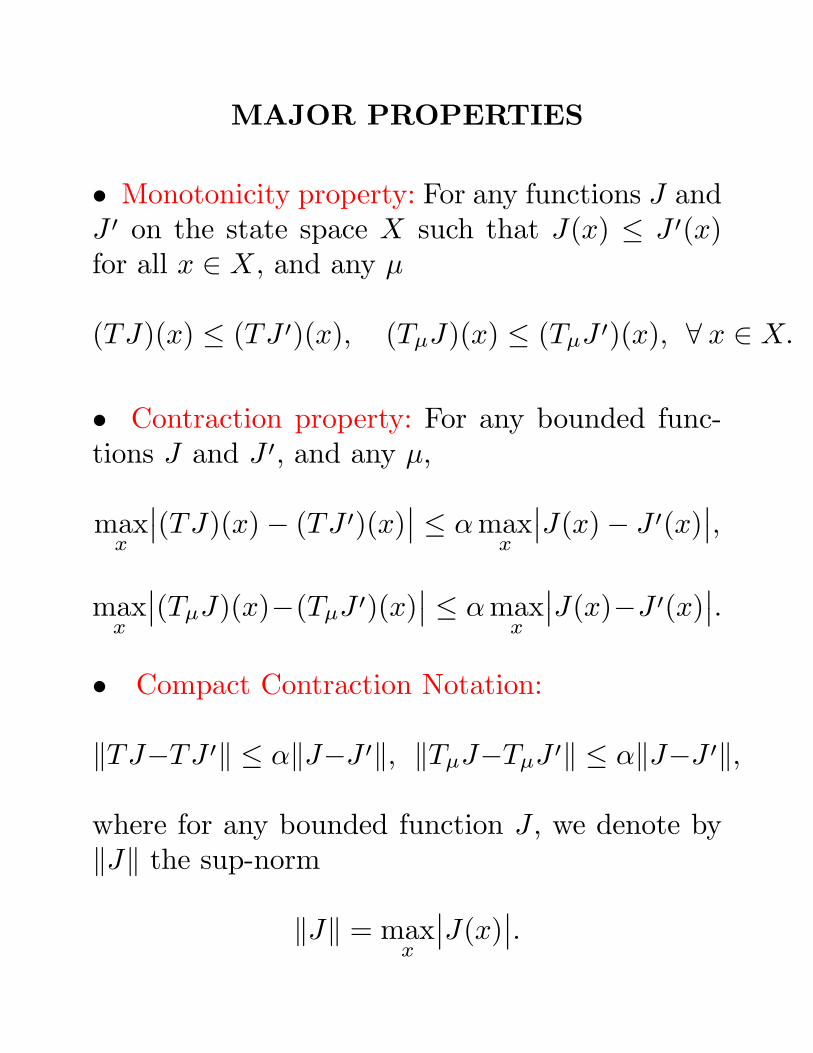
MAJOR PROPERTIES

• Monotonicity property: For any functions J andJ ′ on the state space X such that J(x) ≤ J ′(x)for all x ∈ X, and any µ

(TJ)(x) ≤ (TJ ′)(x), (TµJ)(x) ≤ (TµJ ′)(x), ∀ x ∈ X.

• Contraction property: For any bounded func-tions J and J ′, and any µ,

maxx

∣

∣(TJ)(x)− (TJ ′)(x)∣

∣ ≤ αmaxx

∣

∣J(x)− J ′(x)∣

∣,

maxx

∣

∣(TµJ)(x)−(TµJ ′)(x)∣

∣ ≤ αmaxx

∣

∣J(x)−J ′(x)∣

∣.

• Compact Contraction Notation:

‖TJ−TJ ′‖ ≤ α‖J−J ′‖, ‖TµJ−TµJ ′‖ ≤ α‖J−J ′‖,

where for any bounded function J , we denote by‖J‖ the sup-norm

‖J‖ = maxx

∣

∣J(x)∣

∣.

THE TWO MAIN ALGORITHMS: VI AND PI

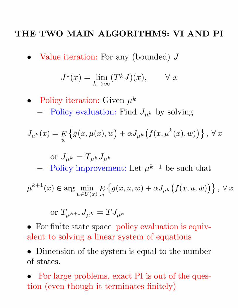
• Value iteration: For any (bounded) J

J∗(x) = limk→∞

(T kJ)(x), ∀ x

• Policy iteration: Given µk

− Policy evaluation: Find Jµk by solving

Jµk (x) = Ew

{

g(

x, µ(x), w)

+ αJµk

(

f(x, µk(x), w))}

, ∀ x

or Jµk = TµkJµk

− Policy improvement: Let µk+1 be such that

µk+1(x) ∈ arg min

u∈U(x)Ew

{

g(x, u, w) + αJµk

(

f(x, u, w))}

, ∀ x

or Tµk+1Jµk = TJµk

• For finite state space policy evaluation is equiv-alent to solving a linear system of equations

• Dimension of the system is equal to the numberof states.

• For large problems, exact PI is out of the ques-tion (even though it terminates finitely)

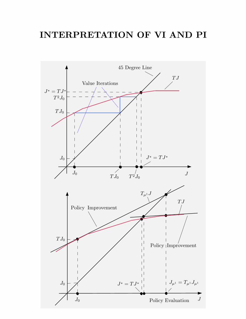
INTERPRETATION OF VI AND PI

J J∗ = TJ∗

0 Prob. = 1

J J∗ = TJ∗

0 Prob. = 1

∗ TJ

Prob. = 1 Prob. =

∗ TJ

Prob. = 1 Prob. =

1 J J

TJ 45 Degree Line

Prob. = 1 Prob. =

J J∗ = TJ∗

0 Prob. = 1

1 J J

J Jµ1 = Tµ1Jµ1

Policy Improvement Exact Policy Evaluation Approximate Policy

Evaluation

Policy Improvement Exact Policy Evaluation Approximate Policy

Evaluation

TJ Tµ1J J

Policy Improvement Exact Policy Evaluation (Exact if

J0

J0

J0

J0

= TJ0

= TJ0

= TJ0

Do not Replace Set S

= T 2J0

Do not Replace Set S

= T 2J0

n Value Iterations

JUSTIFICATION OF POLICY ITERATION

• We can show that Jµk+1 ≤ Jµk for all k

• Proof: For given k, we have

Tµk+1Jµk = TJµk ≤ TµkJµk = Jµk

Using the monotonicity property of DP,

Jµk ≥ Tµk+1Jµk ≥ T 2µk+1Jµk ≥ · · · ≥ lim

N→∞TNµk+1Jµk

• Sincelim

N→∞TNµk+1Jµk = Jµk+1

we have Jµk ≥ Jµk+1 .

• If Jµk = Jµk+1 , all above inequalities holdas equations, so Jµk solves Bellman’s equation.Hence Jµk = J∗

• Thus at iteration k either the algorithm gen-erates a strictly improved policy or it finds an op-timal policy

• For a finite spaces MDP, there are finitely manystationary policies, so the algorithm terminateswith an optimal policy

APPROXIMATE PI

• Suppose that the policy evaluation is approxi-mate,

‖Jk − Jµk‖ ≤ δ, k = 0, 1, . . .

and policy improvement is approximate,

‖Tµk+1Jk − TJk‖ ≤ ǫ, k = 0, 1, . . .

where δ and ǫ are some positive scalars.

• Error Bound I: The sequence {µk} generatedby approximate policy iteration satisfies

lim supk→∞

‖Jµk − J∗‖ ≤ǫ+ 2αδ

(1− α)2

• Typical practical behavior: The method makessteady progress up to a point and then the iteratesJµk oscillate within a neighborhood of J∗.

• Error Bound II: If in addition the sequence {µk}“terminates” at µ (i.e., keeps generating µ)

‖Jµ − J∗‖ ≤ǫ+ 2αδ

1− α

OPTIMISTIC POLICY ITERATION

• Optimistic PI (more efficient): This is PI, wherepolicy evaluation is done approximately, with afinite number of VI

• So we approximate the policy evaluation

Jµ ≈ Tmµ J

for some number m ∈ [1,∞) and initial J

• Shorthand definition: For some integers mk

TµkJk = TJk, Jk+1 = Tmk

µk Jk, k = 0, 1, . . .

• If mk ≡ 1 it becomes VI

• If mk = ∞ it becomes PI

• Can be shown to converge (in an infinite numberof iterations)

• Typically works faster than VI and PI (forlarge problems)

Q-LEARNING I

• We can write Bellman’s equation as

J∗(x) = minu∈U(x)

Q∗(x, u), ∀ x,

where Q∗ is the unique solution of

Q∗(x, u) = E

{

g(x, u, w) + α minv∈U(x)

Q∗(x, v)

}

with x = f(x, u, w)

• Q∗(x, u) is called the optimal Q-factor of (x, u)

• We can equivalently write the VI method as

Jk+1(x) = minu∈U(x)

Qk+1(x, u), ∀ x,

where Qk+1 is generated by

Qk+1(x, u) = E

{

g(x, u, w) + α minv∈U(x)

Qk(x, v)

}

with x = f(x, u, w)

Q-LEARNING II

• Q-factors are no different than costs

• They satisfy a Bellman equation Q = FQ where

(FQ)(x, u) = E

{

g(x, u, w) + α minv∈U(x)

Q(x, v)

}

where x = f(x, u, w)

• VI and PI for Q-factors are mathematicallyequivalent to VI and PI for costs

• They require equal amount of computation ...they just need more storage

• Having optimal Q-factors is convenient whenimplementing an optimal policy on-line by

µ∗(x) = minu∈U(x)

Q∗(x, u)

• Once Q∗(x, u) are known, the model [g andE{·}] is not needed. Model-free operation.

• Later we will see how stochastic/sampling meth-ods can be used to calculate (approximations of)Q∗(x, u) using a simulator of the system (no modelneeded)

A MORE GENERAL/ABSTRACT VIEW OF DP

• Let Y be a real vector space with a norm ‖ · ‖

• A function F : Y 7→ Y is said to be a contrac-tion mapping if for some ρ ∈ (0, 1), we have

‖Fy − Fz‖ ≤ ρ‖y − z‖, for all y, z ∈ Y.

ρ is called the modulus of contraction of F .

• Important example: Let X be a set (e.g., statespace in DP), v : X 7→ ℜ be a positive-valuedfunction. Let B(X) be the set of all functionsJ : X 7→ ℜ such that J(x)/v(x) is bounded overx.

• We define a norm on B(X), called the weightedsup-norm, by

‖J‖ = maxx∈X

|J(x)|

v(x).

• Important special case: The discounted prob-lem mappings T and Tµ [for v(x) ≡ 1, ρ = α].

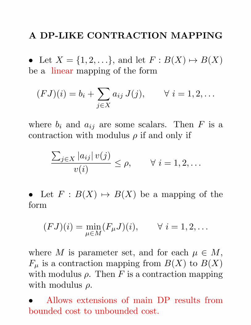
A DP-LIKE CONTRACTION MAPPING

• Let X = {1, 2, . . .}, and let F : B(X) 7→ B(X)be a linear mapping of the form

(FJ)(i) = bi +∑

j∈X

aij J(j), ∀ i = 1, 2, . . .

where bi and aij are some scalars. Then F is acontraction with modulus ρ if and only if

∑

j∈X |aij | v(j)

v(i)≤ ρ, ∀ i = 1, 2, . . .

• Let F : B(X) 7→ B(X) be a mapping of theform

(FJ)(i) = minµ∈M

(FµJ)(i), ∀ i = 1, 2, . . .

where M is parameter set, and for each µ ∈ M ,Fµ is a contraction mapping from B(X) to B(X)with modulus ρ. Then F is a contraction mappingwith modulus ρ.

• Allows extensions of main DP results frombounded cost to unbounded cost.

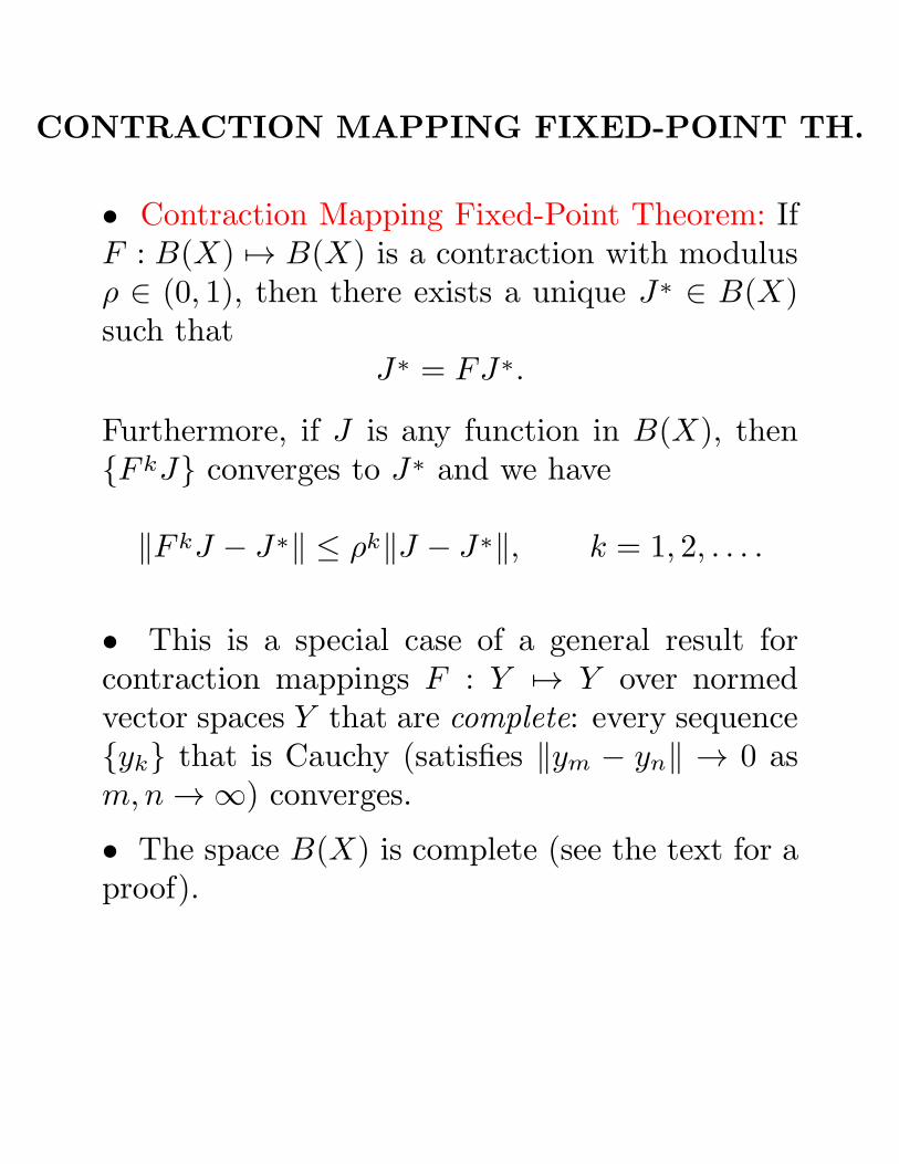
CONTRACTION MAPPING FIXED-POINT TH.

• Contraction Mapping Fixed-Point Theorem: IfF : B(X) 7→ B(X) is a contraction with modulusρ ∈ (0, 1), then there exists a unique J∗ ∈ B(X)such that

J∗ = FJ∗.

Furthermore, if J is any function in B(X), then{F kJ} converges to J∗ and we have

‖F kJ − J∗‖ ≤ ρk‖J − J∗‖, k = 1, 2, . . . .

• This is a special case of a general result forcontraction mappings F : Y 7→ Y over normedvector spaces Y that are complete: every sequence{yk} that is Cauchy (satisfies ‖ym − yn‖ → 0 asm,n → ∞) converges.

• The space B(X) is complete (see the text for aproof).

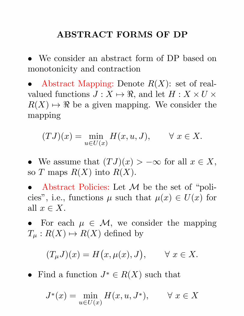
ABSTRACT FORMS OF DP

• We consider an abstract form of DP based onmonotonicity and contraction

• Abstract Mapping: Denote R(X): set of real-valued functions J : X 7→ ℜ, and let H : X ×U ×R(X) 7→ ℜ be a given mapping. We consider themapping

(TJ)(x) = minu∈U(x)

H(x, u, J), ∀ x ∈ X.

• We assume that (TJ)(x) > −∞ for all x ∈ X,so T maps R(X) into R(X).

• Abstract Policies: Let M be the set of “poli-cies”, i.e., functions µ such that µ(x) ∈ U(x) forall x ∈ X.

• For each µ ∈ M, we consider the mappingTµ : R(X) 7→ R(X) defined by

(TµJ)(x) = H(

x, µ(x), J)

, ∀ x ∈ X.

• Find a function J∗ ∈ R(X) such that

J∗(x) = minu∈U(x)

H(x, u, J∗), ∀ x ∈ X

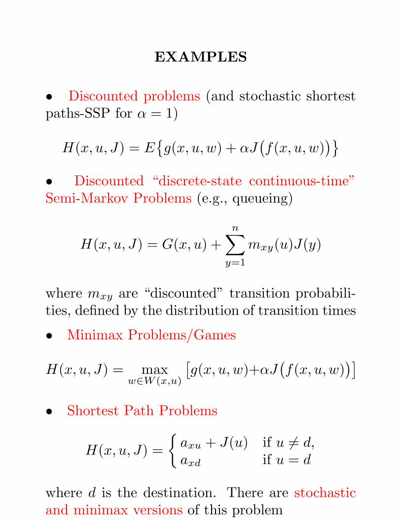
EXAMPLES

• Discounted problems (and stochastic shortestpaths-SSP for α = 1)

H(x, u, J) = E{

g(x, u, w) + αJ(

f(x, u, w))}

• Discounted “discrete-state continuous-time”Semi-Markov Problems (e.g., queueing)

H(x, u, J) = G(x, u) +n∑

y=1

mxy(u)J(y)

where mxy are “discounted” transition probabili-ties, defined by the distribution of transition times

• Minimax Problems/Games

H(x, u, J) = maxw∈W (x,u)

[

g(x, u, w)+αJ(

f(x, u, w))]

• Shortest Path Problems

H(x, u, J) =

{

axu + J(u) if u 6= d,axd if u = d

where d is the destination. There are stochasticand minimax versions of this problem

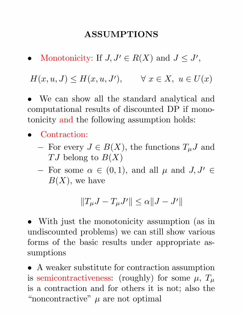
ASSUMPTIONS

• Monotonicity: If J, J ′ ∈ R(X) and J ≤ J ′,

H(x, u, J) ≤ H(x, u, J ′), ∀ x ∈ X, u ∈ U(x)

• We can show all the standard analytical andcomputational results of discounted DP if mono-tonicity and the following assumption holds:

• Contraction:

− For every J ∈ B(X), the functions TµJ andTJ belong to B(X)

− For some α ∈ (0, 1), and all µ and J, J ′ ∈B(X), we have

‖TµJ − TµJ ′‖ ≤ α‖J − J ′‖

• With just the monotonicity assumption (as inundiscounted problems) we can still show variousforms of the basic results under appropriate as-sumptions

• A weaker substitute for contraction assumptionis semicontractiveness: (roughly) for some µ, Tµ

is a contraction and for others it is not; also the“noncontractive” µ are not optimal

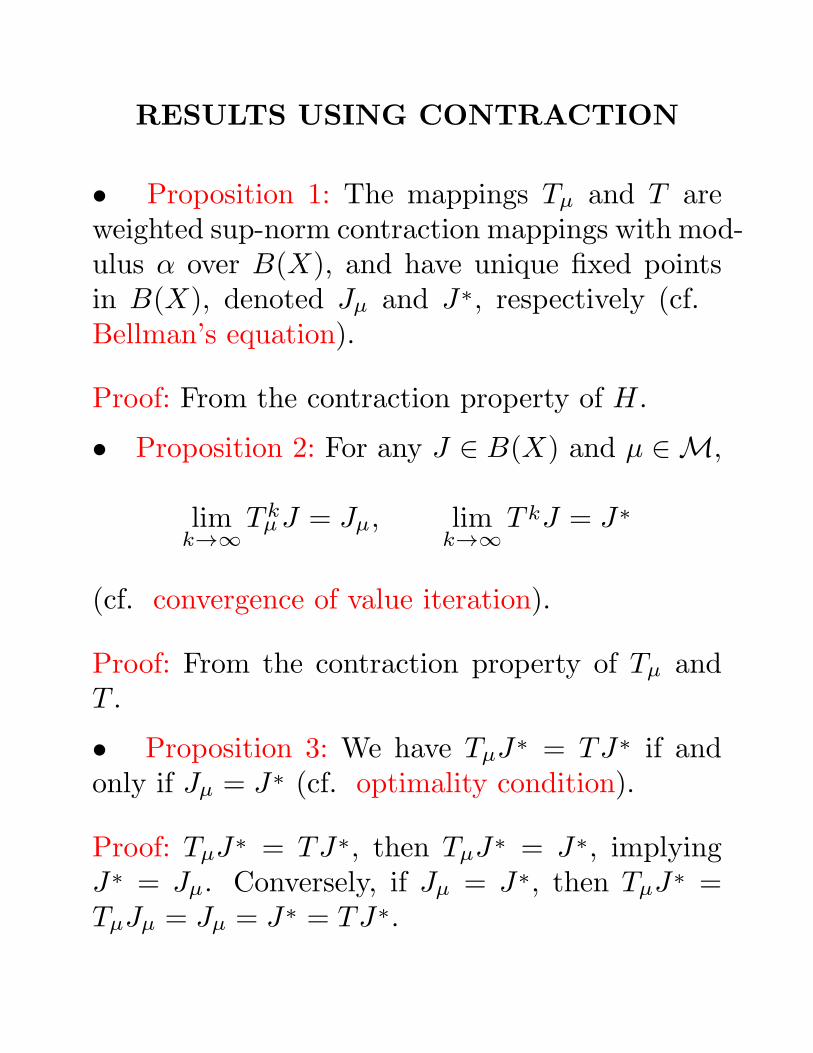
RESULTS USING CONTRACTION

• Proposition 1: The mappings Tµ and T areweighted sup-norm contraction mappings with mod-ulus α over B(X), and have unique fixed pointsin B(X), denoted Jµ and J∗, respectively (cf.Bellman’s equation).

Proof: From the contraction property of H .

• Proposition 2: For any J ∈ B(X) and µ ∈ M,

limk→∞

T kµJ = Jµ, lim

k→∞T kJ = J∗

(cf. convergence of value iteration).

Proof: From the contraction property of Tµ andT .

• Proposition 3: We have TµJ∗ = TJ∗ if andonly if Jµ = J∗ (cf. optimality condition).

Proof: TµJ∗ = TJ∗, then TµJ∗ = J∗, implyingJ∗ = Jµ. Conversely, if Jµ = J∗, then TµJ∗ =TµJµ = Jµ = J∗ = TJ∗.

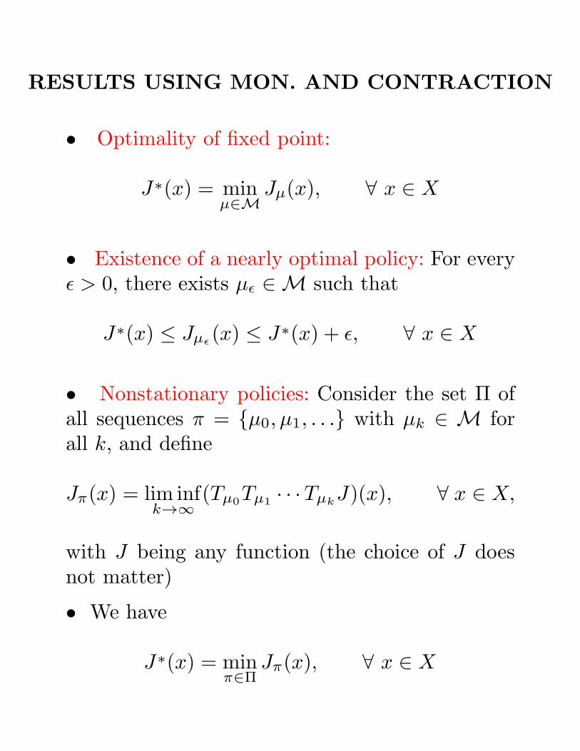
RESULTS USING MON. AND CONTRACTION

• Optimality of fixed point:

J∗(x) = minµ∈M

Jµ(x), ∀ x ∈ X

• Existence of a nearly optimal policy: For everyǫ > 0, there exists µǫ ∈ M such that

J∗(x) ≤ Jµǫ(x) ≤ J∗(x) + ǫ, ∀ x ∈ X

• Nonstationary policies: Consider the set Π ofall sequences π = {µ0, µ1, . . .} with µk ∈ M forall k, and define

Jπ(x) = lim infk→∞

(Tµ0Tµ1

· · ·TµkJ)(x), ∀ x ∈ X,

with J being any function (the choice of J doesnot matter)

• We have

J∗(x) = minπ∈Π

Jπ(x), ∀ x ∈ X

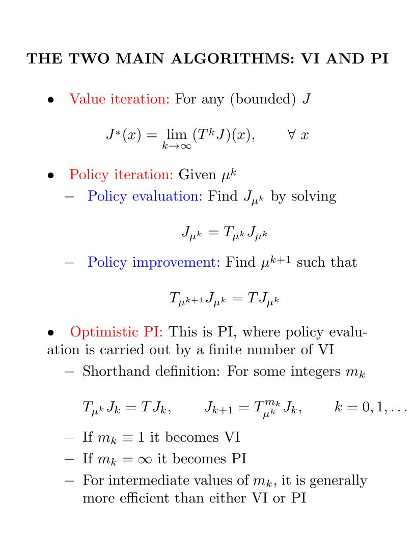
THE TWO MAIN ALGORITHMS: VI AND PI

• Value iteration: For any (bounded) J

J∗(x) = limk→∞

(T kJ)(x), ∀ x

• Policy iteration: Given µk

− Policy evaluation: Find Jµk by solving

Jµk = TµkJµk

− Policy improvement: Find µk+1 such that

Tµk+1Jµk = TJµk

• Optimistic PI: This is PI, where policy evalu-ation is carried out by a finite number of VI

− Shorthand definition: For some integers mk

TµkJk = TJk, Jk+1 = Tmk

µk Jk, k = 0, 1, . . .

− If mk ≡ 1 it becomes VI

− If mk = ∞ it becomes PI

− For intermediate values of mk, it is generallymore efficient than either VI or PI

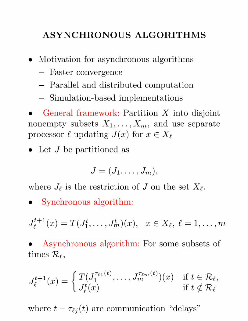
ASYNCHRONOUS ALGORITHMS

• Motivation for asynchronous algorithms

− Faster convergence

− Parallel and distributed computation

− Simulation-based implementations

• General framework: Partition X into disjointnonempty subsets X1, . . . , Xm, and use separateprocessor ℓ updating J(x) for x ∈ Xℓ

• Let J be partitioned as

J = (J1, . . . , Jm),

where Jℓ is the restriction of J on the set Xℓ.

• Synchronous algorithm:

J t+1ℓ (x) = T (J t

1, . . . , Jtm)(x), x ∈ Xℓ, ℓ = 1, . . . ,m

• Asynchronous algorithm: For some subsets oftimes Rℓ,

J t+1ℓ (x) =

{

T (Jτℓ1(t)1 , . . . , J

τℓm(t)m )(x) if t ∈ Rℓ,

J tℓ(x) if t /∈ Rℓ

where t− τℓj(t) are communication “delays”

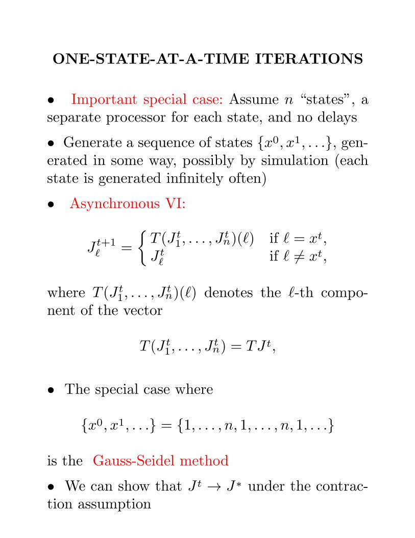
ONE-STATE-AT-A-TIME ITERATIONS

• Important special case: Assume n “states”, aseparate processor for each state, and no delays

• Generate a sequence of states {x0, x1, . . .}, gen-erated in some way, possibly by simulation (eachstate is generated infinitely often)

• Asynchronous VI:

J t+1ℓ =

{

T (J t1, . . . , J

tn)(ℓ) if ℓ = xt,

J tℓ if ℓ 6= xt,

where T (J t1, . . . , J

tn)(ℓ) denotes the ℓ-th compo-

nent of the vector

T (J t1, . . . , J

tn) = TJ t,

• The special case where

{x0, x1, . . .} = {1, . . . , n, 1, . . . , n, 1, . . .}

is the Gauss-Seidel method

• We can show that J t → J∗ under the contrac-tion assumption

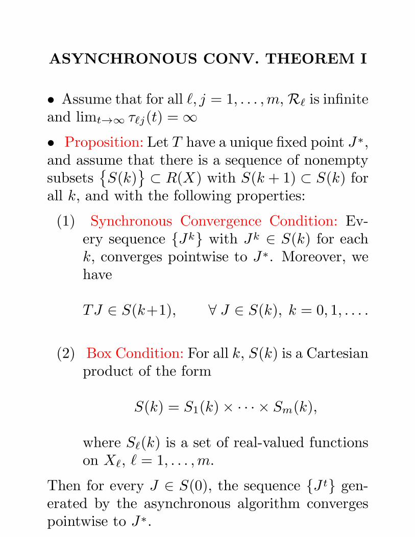
ASYNCHRONOUS CONV. THEOREM I

• Assume that for all ℓ, j = 1, . . . ,m, Rℓ is infiniteand limt→∞ τℓj(t) = ∞

• Proposition: Let T have a unique fixed point J∗,and assume that there is a sequence of nonemptysubsets

{

S(k)}

⊂ R(X) with S(k + 1) ⊂ S(k) forall k, and with the following properties:

(1) Synchronous Convergence Condition: Ev-ery sequence {Jk} with Jk ∈ S(k) for eachk, converges pointwise to J∗. Moreover, wehave

TJ ∈ S(k+1), ∀ J ∈ S(k), k = 0, 1, . . . .

(2) Box Condition: For all k, S(k) is a Cartesianproduct of the form

S(k) = S1(k)× · · · × Sm(k),

where Sℓ(k) is a set of real-valued functionson Xℓ, ℓ = 1, . . . ,m.

Then for every J ∈ S(0), the sequence {J t} gen-erated by the asynchronous algorithm convergespointwise to J∗.

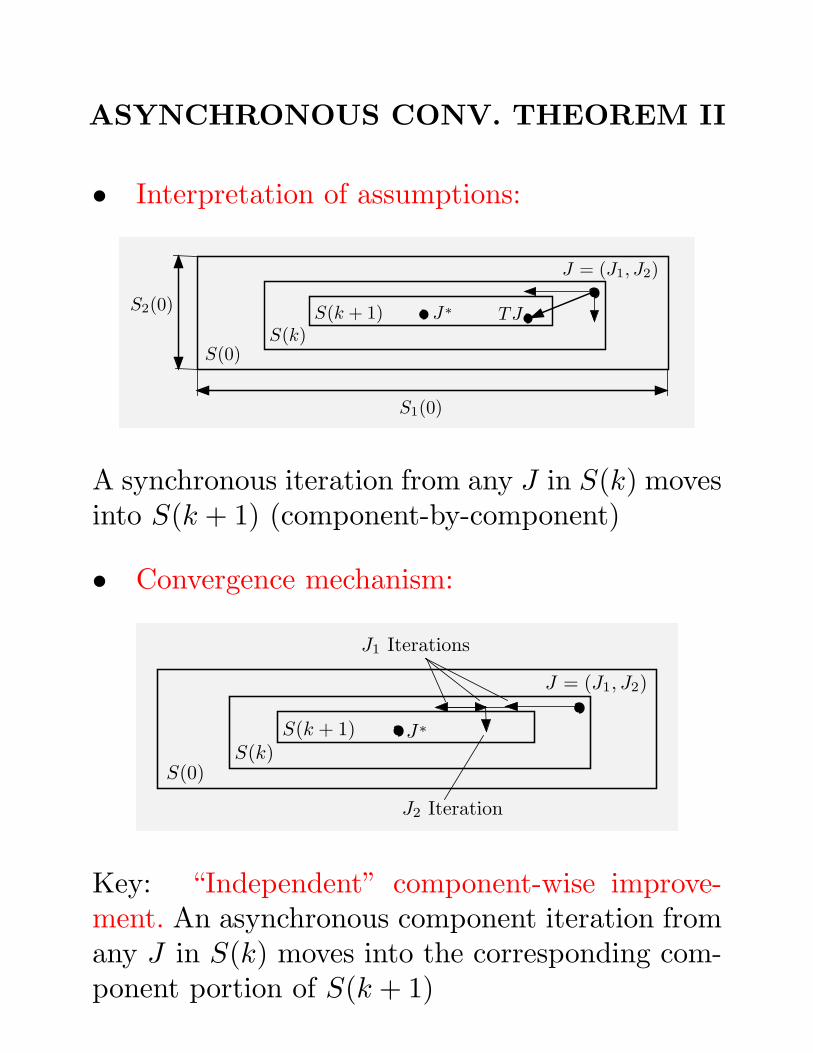
ASYNCHRONOUS CONV. THEOREM II

• Interpretation of assumptions:

S(0)(0) S(k)

) S(k + 1) + 1) J∗

∗ J = (J1, J2)

S1(0)

(0) S2(0)TJ

A synchronous iteration from any J in S(k) movesinto S(k + 1) (component-by-component)

• Convergence mechanism:

S(0)(0) S(k)

) S(k + 1) + 1) J∗

∗ J = (J1, J2)

J1 Iterations

Iterations J2 Iteration

Key: “Independent” component-wise improve-ment. An asynchronous component iteration fromany J in S(k) moves into the corresponding com-ponent portion of S(k + 1)