Embed Size (px)
Citation preview

1
An Automated Method for Depicting 1
Mesocyclone Paths and Intensities 2
3
4
Madison L. Miller1 5
6
Cooperative Institute of Mesoscale Meteorological Studies, University of 7
Oklahoma and National Severe Storms Laboratory, Norman, Oklahoma 8
9
Valliappa Lakshmanan 10
11
Cooperative Institute of Mesoscale Meteorological Studies, University of 12
Oklahoma and National Severe Storms Laboratory, Norman, Oklahoma 13
14
Travis M. Smith 15
16
Cooperative Institute of Mesoscale Meteorological Studies, University of 17
Oklahoma and National Severe Storms Laboratory, Norman, Oklahoma 18
19
20
21
22
23
24
25
Accepted by Weather and Forecasting, Nov. 2012 26
27
28
29
30
31
32
33
34
35 1Corresponding author address: Madison L. Miller, School of Meteorology, University of Oklahoma, 120 36
David L. Boren Blvd., Norman, OK 73072. 37 E-mail: [email protected] 38
39

2
Abstract 40
41
The location and intensity of mesocyclone circulations can be tracked in real-time by 42
accumulating azimuthal shear values over time at every location of a uniform spatial grid. 43
Azimuthal shear at low (0-3 km AGL) and mid levels (3-6 km AGL) of the atmosphere is 44
computed in a noise-tolerant manner by fitting the Doppler velocity observations in the 45
neighborhood of a pulse volume to a plane and finding the slope of that plane. Rotation 46
tracks created in this manner are contaminated by non-meteorological signatures caused 47
by poor velocity dealiasing, ground clutter, radar test patterns and spurious shear values. 48
In order to improve the quality of these fields for real-time use and for an accumulated 49
multi-year climatology, new dealiasing strategies, data thresholding, and Multiple 50
Hypothesis Tracking (MHT) techniques have been implemented. These techniques 51
remove nearly all non-meteorological contaminants resulting in much clearer rotation 52
tracks that appear to match mesocyclone paths and intensities closely. 53

3
1. Introduction 54
a. Motivation 55
To depict the paths and intensities of mesocyclone circulations as seen by radar, 56
the National Severe Storms Laboratory (NSSL) creates products called “rotation tracks”. 57
These rotation track fields are created by calculating the azimuthal shear fields (the 58
azimuthal derivative of radial velocity) for each radar, merging the azimuthal shear data 59
from multiple radars onto Cartesian grids and then accumulating the maximum values in 60
those gridded fields over time onto one accumulated grid. An example is shown in Figure 61
1. 62
These tracks can help alleviate some of the difficulty in interpreting and analyzing 63
velocity fields. They can provide information about the spatial extent and strength of 64
mesocyclone signatures over time and can be quite useful for conducting poststorm 65
damage surveys. The American Red Cross of Central Oklahoma uses NSSL rotation 66
track products plotted on maps to determine where to deliver assistance after tornado 67
events and the best routes to get there. After the 24 May 2011 tornado outbreak in Central 68
Oklahoma, the use of rotation tracks helped to significantly reduce the disaster 69
assessment time (NOAA/NSSL 2011). These fields are also useful in real-time as 70
guidance for forecasters and have enormous data mining potential. However, they are 71
plagued by non-meteorological signatures caused by poor velocity dealiasing, ground 72
clutter, radar test patterns, and spurious shear values. As seen in Figure 2, these artifacts 73
can make the tracks difficult, if not impossible, to interpret meaningfully. 74
One of the goals of the Multi-Year Reanalysis of Remotely Sensed Storms 75
(MYRORSS) project, a cooperative effort between National Oceanic and Atmospheric 76
4
Administration’s (NOAA) NSSL and the National Climatic Data Center (NCDC), is to 77
create a CONUS-wide climatology of low and mid level rotation track fields for the 78
lifetime of the Weather Surveillance Radar 1988-Doppler (WSR-88D) network. 79
Cintineo et al. (2011) developed an automated system to process Level-II radar 80
data (Crum and Alberty 1993) at NSSL using a multiple-machine framework and the 81
Warning Decision Support System – Integrated Information (WDSS-II; Lakshmanan et 82
al. 2007b) suite of programs to process and quality control the data. A preliminary hail 83
climatology using Maximum Estimated Size of Hail (MESH) grids was also created. 84
Here, we extend the processing to velocity-based products, specifically to azimuthal 85
shear accumulations. 86
The CONUS-wide rotation track climatology will provide an incredibly rich 87
dataset with numerous potential climatological and severe weather applications. Track 88
lengths, intensities, and other characteristics could be analyzed by geographical region 89
and time of year. Potential relationships could also be discovered between rotation tracks 90
and environmental parameters like convective available potential energy (CAPE) and 91
storm-relative helicity (SRH). After correlating maximum azimuthal shear and maximum 92
updraft helicity, rotation tracks could also be used as verification for high-resolution 93
model-simulated maximum updraft helicity tracks like the ones discussed by Kain et al. 94
(2010) and Clark et al. (2012). 95
The purpose of this paper is to discuss the special velocity dealiasing techniques, 96
data thresholds, and Multiple Hypothesis Tracking (MHT) techniques developed to 97
isolate the rotation tracks in real-time and for the MYRORSS climatology. Detailed 98

5
explanations of each quality control effort will be given and the specific impacts of each 99
step will be shown in example cases. 100
b. Background 101
Modern Doppler radars have the ability to provide high resolution space and time 102
measurements of storms that allow for the detection of mesocyclone-scale circulations. 103
Couplets in radial velocity fields as well as hook echo signatures in reflectivity fields 104
have been used to identify these circulations in the past, but methods of identifying 105
mesocyclone or tornado circulations reliant solely on hook echo signatures have proven 106
unreliable (Forbes 1981; Mitchell et al. 1998). Methods using radial velocity signatures 107
such as the Tornado Detection Algorithm (TDA; Mitchell et. al 1998) and the NSSL 108
Mesocyclone Detection Algorithm (MDA; Stumpf et. al 1998) have been more 109
successful. 110
The TDA currently used with the WSR-88D system relies on high “gate-to-gate 111
velocity difference” values to identify potentially tornadic circulations (Mitchell et al. 112
1998). Although termed a tornado detector, the algorithm identifies tornadic vortex 113
signatures (which may or may not be associated with tornadoes) that are typically larger 114
than a tornado owing to radar sampling resolution (e.g., Brown et al. 1978). The gate-to-115
gate difference represents the difference between velocity values at constant range from 116
the radar between adjacent azimuths. These values can be affected adversely by the 117
azimuthal offset of the radar beam center from the vortex, noisy data, and velocity 118
aliasing (Wood and Brown 1997). Additionally, because the radar beam is much broader 119
at far ranges than when near the radar, observed velocity peaks within vortices decrease 120
in magnitude, allowing some vortices to be overlooked by the algorithm. 121

6
Liu et al. (2007) proposed a wavelet analysis technique to help mitigate these 122
issues. The method examines region-to-region radial wind shears at a number of different 123
spatial scales to more accurately determine the amount of shear present, reducing the 124
number of false tornado detections. 125
Rather than using the gate-to-gate velocity difference, “peak-to-peak” methods of 126
calculating rotational shear from Doppler radial velocity data or the wavelet analysis 127
technique to detect a vortex, a two-dimensional, local, linear least squares derivatives 128
(LLSD) method can be used to reduce the impact of noise. Elmore et al. (1994) proposed 129
this method of estimating the derivatives of radial velocity values by fitting a plane to the 130
velocity field and finding its slope. The vertical vorticity field is estimated by the 131
azimuthal derivative of the radial velocity field and is given by 132
∑
∑( )
(1)
where is the radial velocity, is the coordinate in the azimuthal direction, is the arc 133
length from the center point of the calculation to the point ( ) is the radial velocity 134
at point ( ), and is the beam width at a given range. is a positive weight 135
function that we set to 1 after determining that Cressman weight functions, among others, 136
generated very little differences. The coordinate is in the radial direction and is in the 137
azimuthal direction. The summation is performed over range gates in the neighborhood 138
of the starting point of the calculation. This calculation of azimuthal shear is, here on, 139
referred to as the LLSD method. 140
Smith and Elmore (2004) applied the LLSD calculation to simulated and observed 141
circulations by first passing the velocity data through a 3x3 median filter (Lakshmanan 142

7
2012) to reduce speckle noise and then applying Eq.1 to the filtered velocity data to 143
estimate the azimuthal shear. The physical size of the neighborhood used in the 144
calculation is held constant such that fewer radials are used in the calculation at far 145
ranges from the radar. Typical sizes of radial and azimuthal neighborhoods are 750 m and 146
2500 m, respectively. 147
The LLSD calculation helps to remove some of the dependence on radar location 148
involved in rotation detection and also allows circulation signatures to be viewed in 149
three-dimensional space or as input to multi-sensor applications. It was shown by Smith 150
and Elmore (2004) that LLSD shear values were reasonable estimations of actual shear 151
values in simulated Rankine vortices when sampled by a theoretical WSR-88D radar 152
(Brown et al. 2002) out to a range of ~140 km. The variance of these values was also 153
much smaller compared to peak-to-peak shear. 154
The use of the median filter in the LLSD shear technique can be a disadvantage, 155
however. Whereas areas with large velocity gradients are preserved, this filter can also 156
smooth out peaks in the velocity field. Although the median filter is beneficial when 157
these peaks are associated with noisy data, the filter decreases the magnitude of peak 158
velocities in mesocyclone signatures and completely eliminates tornado signatures in 159
nearly all cases. For this reason, LLSD shear values may underestimate the actual 160
azimuthal shear of circulations, especially for small circulations (Mitchell and Elmore 161
1998). 162
Defining a neighborhood size in the LLSD technique also forces a trade-off 163
between spatial resolution and noise resistance. Smaller neighborhoods are more strongly 164
affected by noise, whereas larger neighborhoods tend to underestimate actual shear 165

8
values of circulations. The spatial scale of the LLSD calculation makes it most useful for 166
detecting large mesocyclone-scale circulations, however, the increased noise resistance 167
makes identification of small circulations more difficult. 168
Rotation tracks help to visualize the movement of mesocyclone circulations (or 169
occasionally circulations associated with nearby large tornadoes) over time as seen by 170
radar. To produce these tracks, radial velocity data are first dealiased using the default 171
WSR-88D dealiasing algorithm (Eilts and Smith 1990). Next, a quality control neural 172
network (Lakshmanan et al. 2007a) is used to remove echoes in the reflectivity field 173
produced by biological targets, anomalous propagation, ground clutter, and test or 174
interference patterns. The algorithm successfully removes nearly all non-meteorological 175
signatures from the Reflectivity fields examined. 176
This quality controlled reflectivity field, hereafter ReflectivityQC, and the radial 177
velocity field are then employed by the shear estimation algorithm of Smith and Elmore 178
(2004) to compute the azimuthal shear (see Fig. 3). Two-dimensional maximum 179
azimuthal shear fields within low (0-3 km) and mid (3-6 km) level layers above ground 180
level (AGL) are also calculated using digital elevation model (DEM) data to determine 181
the height of each point above the ground. 182
These single-radar 2-D maximum azimuthal shear fields are then merged into a 183
Cartesian multi-radar grid using the intelligent agent formulation of Lakshmanan et al. 184
(2006), accounting for varying radar beam geometry with range, vertical gaps between 185
radar scans, and other issues. The maximum value of each pixel in the merged multi-186
radar grid over a time interval (typically 60 -120 minutes) is then used to produce the 187
swaths of merged maximum azimuthal shear known as rotation tracks. Missing data in 188

9
the rotation track fields (denoted by “MD” in the color bar) corresponds to any data 189
below the signal to noise threshold for the radar. Ideally, this should be shown as zero 190
shear, not missing data. Figure 4 provides a flow chart showing the algorithms and fields 191
used to create rotation tracks. 192
2. Methods 193
a. Two-dimensional velocity dealiasing 194
Due to the relationship between radar wave length ( ) and the pulse repetition 195
frequency ( ), a radar correctly measures the radial velocity given that it is in the range 196
of , where 197
(2)
Here, is the Nyquist velocity and the true velocity is 198
(3)
where is the measured velocity, is an unknown integer including zero, and must 199
satisfy . Velocity dealiasing is the process of determining the correct 200
value of n to successfully recover . In the cases when cannot be successfully 201
recovered, the velocity is still aliased and can usually be identified in radial velocity 202
fields by abrupt changes in values between neighboring measurements. Most first 203
generation dealiasing algorithms (e.g. Ray and Ziegler 1977, Bargen and Brown 1980) 204
were one-dimensional and detected abrupt changes between single radials. For this 205
reason, they were quite sensitive to noisy, incorrect data. Strong shear zones in these 206
radial velocity fields sometimes cannot be dealiased without data from multiple 207
10
dimensions. Merritt (1984), Boren et al. (1986), and Bergen and Albers (1988) took more 208
sophisticated approaches and used velocity data in two dimensions to dealias. These 209
methods were costly in terms of computation time, however. 210
The local environment dealiasing (LED) algorithm (Eilts and Smith 1990) is the 211
method currently used for WSR-88D data in real-time. The scheme applies radial 212
continuity constraints to remove local aliasing errors and azimuthal continuity checks to 213
mitigate error. It also incorporates radial averages to determine n (see Eq. 3) when 214
continuity thresholds are not met. Each radial is processed individually and compared 215
against the previously dealiased radials, allowing the algorithm to use less memory and 216
process faster than other two-dimensional algorithms. It can also ingest a vertical wind 217
profile from an environmental sounding to produce initial values for each elevation scan 218
and for isolated echoes. It is an efficient algorithm that begins by using simple checks and 219
only moves on to more sophisticated techniques if needed. This approach performed very 220
well on the cases of severe aliasing presented in Eilts and Smith (1990), but performed 221
poorly when qualitatively examined in many of the tornadic cases examined for this 222
study. Ingesting the vertical wind field from a 20-km Rapid Update Cycle model (RUC; 223
Benjamin et al. 2004) point sounding at each radar site to use as an environmental 224
estimate into the LED algorithm improved the dealiasing to some extent. 225
For this study, a sophisticated two-dimensional dealiasing technique described by 226
Jing and Wiener (1993) was implemented. The algorithm solves a linear system of 227
equations that minimizes gate-to-gate shear in each isolated two-dimensional region. 228
Through using aliasing-induced discontinuity information, the correction values for all 229
gates are found by solving a two-dimensional least-mean-squares problem. Instead of 230

11
making dealiasing decisions for each gate based on its neighbors, which can be subject to 231
scattered incorrect data, this approach avoids local expansion of errors by attempting to 232
find all dealiased values for a given dataset. Vertical profiles of horizontal wind data 233
from the 20-km RUC point soundings were used as environmental wind estimates at the 234
grid-point nearest to each radar site. The calculated average is minimized by 235
incrementing equally over the entire echo. The average local wind observed by radar 236
is assumed to be less than . 237
A smooth environmental wind field with weak shear is assumed. This can be a 238
poor assumption in isolated areas of strong wind shear associated with mesocyclones or 239
microbursts. In these cases, relatively short falsely aliased border segments are detected 240
and can typically be used to dealiase the field correctly. In more elongated regions of 241
shear associated with strong gust fronts, for example, incorrect dealiasing is more likely. 242
Example dealiased radial velocity fields and their corresponding azimuthal shear fields 243
using both the LED and Jing and Weiner (1993) methods are shown in Fig. 3. 244
Preliminary results from a study now underway to determine which velocity dealiasing 245
method performs best on a set of case studies indicate that this two-dimensional 246
technique is more accurate than the LED technique. 247
b. Reflectivity quality control 248
As mentioned in the introduction, the quality control neural network 249
(Lakshmanan et al. 2007b, Lakshmanan et al. 2010) is used to remove non-250
meteorological echoes from the reflectivity field. The algorithm combines various 251
measures from both past literature (e.g. Steiner and Smith 2002, Kessinger et al. 2003, 252
Fulton et al. 1998) and new measures to discriminate between precipitating and 253
12
nonprecipitating echoes in the reflectivity data. A region-by-region classification is 254
performed rather than a gate-by-gate basis. In addition, clear air echoes due to biological 255
contamination are identified and removed using a two-stage intelligent machine 256
algorithm while retaining echoes that correspond to precipitation (Lakshmanan et al. 257
2010). 258
c. Additions to LLSD shear algorithm 259
In addition to calculating the azimuthal shear fields as described earlier in this 260
paper, extra operations have been added to the LLSD algorithm. These additions are 261
discussed in the following sections. 262
1) AZIMUTHAL SHEAR RANGE CORRECTION 263
A new azimuthal shear range-correction (Newman et al. 2012) algorithm is 264
applied to the field in an effort to correct for range degradation due to radar beam 265
widening. A multiple linear regression technique was used to create the equations based 266
on comparisons between observed shear values and those computed using simulated 267
Rankine vortices. First, the algorithm identifies significant circulations using reflectivity 268
and LLSD shear criteria. To avoid applying the range-correction to regions of noise in the 269
shear fields co-located with low reflectivity values, only circulations in regions with 270
reflectivity values greater than 20 dBZ and LLSD shear values exceeding 0.005 s-1
are 271
identified. The peak-to-peak velocity differences and shear diameters of circulations 272
satisfying the reflectivity and shear criteria are calculated next. A median filter is applied 273
to the shear diameter field to provide potentially more accurate estimates of circulation 274
size when circulations are larger than tornadic vortex signatures (TVSs; Brown, Lemon, 275

13
and Burgess 1978). Then, new azimuthal shear values for each pixel in the circulations 276
are calculated by inserting the associated shear diameter, maximum velocity measured, 277
and range values into the appropriate regression equations. Newman et al. (2012) found 278
that the algorithm increased tornadic shear values appropriately and aided in the 279
differentiation between tornadic and nontornadic scans. 280
2) DATA THRESHOLDS AND REMOVAL 281
Significant vertical shear near the surface can cause false high azimuthal shear 282
values very close to the radar. To prevent these high values from corrupting the multi-283
year climatology, azimuthal shear values within a 5-km radius of each radar site are set to 284
‘missing’. While this will remove some ‘good’ data, it will also remove a great deal of 285
anomalously high azimuthal shear values that could corrupt the climatology. An example 286
is shown in Figure 5. This near-radar data removal is not applied to the rotation tracks in 287
this paper, nor will it be used in generation of rotation tracks in real-time. It is used only 288
in the climatology to avoid accumulations at areas where the azimuthal shear values are 289
known to be poor. 290
When processing the two-dimensional maximum azimuthal shear fields, all shear 291
data not co-located with a given ReflectivityQC value are removed so that only shear data 292
associated with storm regions are retained. In order to retain meteorologically significant 293
shear data in low reflectivity hook echo regions, a 5x5 dilation filter (Lakshmanan 2012) 294
is applied to the ReflectivityQC field. This operation assigns the maximum reflectivity 295
value in a 5x5 moving window to each pixel, effectively expanding the areas of high 296
reflectivity values. The threshold operation is then performed on the dilated 297
ReflectivityQC field to help remove azimuthal shear associated with interference 298

14
patterns, anomalous propagation, and other radar-related issues not successfully removed 299
by the radar reflectivity quality control neural network. Setting this threshold at 40 dBZ 300
retained the meteorological rotation signatures in the azimuthal shear fields while 301
removing a great deal of shear co-located with non-meteorological signatures (see Figure 302
6). 303
d. Creation of rotation tracks 304
To better isolate the rotation tracks in the accumulated grid, new quality control 305
strategies have been implemented on the input two-dimensional maximum azimuthal 306
shear fields for both low and mid levels of the atmosphere. Clusters of high azimuthal 307
shear values in each time step are tested and removed if their sizes and/or data value 308
distributions are not indicative of meteorological phenomena. If these remaining clusters 309
in each time step are associated with lasting circulations, they make it into the final 310
rotation track products. 311
1) HYSTERESIS SEGMENTATION 312
Before the circulation signatures in the two-dimensional maximum azimuthal 313
shear fields can be associated between time steps, they are isolated into clusters of high 314
shear values using hysteresis segmentation. The term hysteresis (Jain 1989) refers to the 315
lag observed between the application of an electromagnetic field and its subsequent effect 316
on a substance. In image processing, the term refers to the lagging effect caused by using 317
two thresholds – one to begin the thresholding process and another to end it. In this 318
application, two data thresholds are maintained and a cluster is composed of contiguous 319
pixels with values greater than the lower data threshold that contains at least one pixel 320
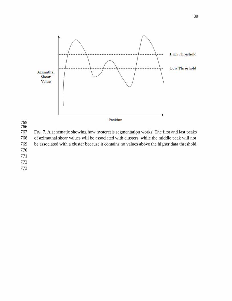
15
with a data value greater than the higher threshold. The higher threshold identifies areas 321
of high azimuthal shear associated with strong circulation and the lower hysteresis 322
threshold grows the region around the high value to include all pixels associated with the 323
circulation (see Figure 7). Through experimentation on numerous tornadic and 324
nontornadic case studies, it was determined that low and high data thresholds of 0.002 s-1
325
and 0.005 s-1
, respectively, and a minimum size of 25 pixels performed well for isolating 326
clusters of high azimuthal shear. 327
All pixels in the maximum 2-D azimuthal shear layer fields not associated with 328
identified clusters are then removed so that only the azimuthal shear clusters are 329
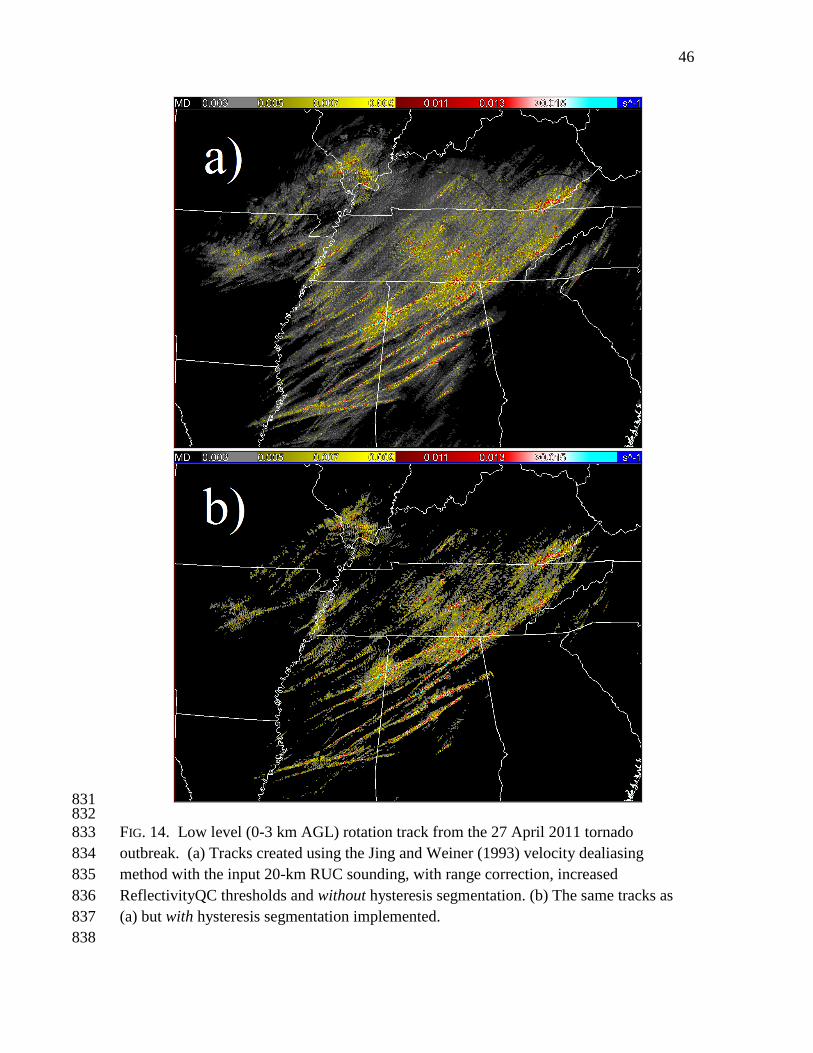
accumulated over time to produce rotation tracks. This eliminates the low background 330
azimuthal shear values not associated with circulations, making the tracks themselves 331
more isolated, as seen in Figure 8. 332
2) MULTIPLE HYPOTHESIS TRACKING 333
Typically, clusters of high azimuthal shear values associated with mesocyclones 334
persist through many time steps, whereas clusters associated with remaining non-335
meteorological signatures typically only appear sporadically. To isolate the 336
meteorological rotation tracks, these non-meteorological shear clusters need to be 337
removed from the accumulated fields. Multiple Hypothesis Tracking (MHT) (Cox and 338
Hingorani 1996) techniques are used to isolate the continuous tracks of azimuthal shear 339
clusters associated with storms and remove the short-lived non-meteorological azimuthal 340
shear clusters. 341
MHT techniques have been used in the fields of video processing and military 342
target tracking for years and recently have been adopted by the meteorology community 343

16
(e.g. Root et al. 2011). The technique attempts to associate objects, in this case azimuthal 344
shear clusters, throughout time. It is innovative as it considers time associations globally 345
and makes association decisions that can be deferred until additional information is 346
available. If the algorithm is not certain whether an existing track should be associated 347
with cluster A or cluster B in the current time step, for example, it can create two 348
hypotheses (see Figure 9). Both possibilities are then propagated forward in time to when 349
enough information should be available to determine which hypothesis most likely. The 350
clusters that do not meet the minimum longevity threshold (two time steps or roughly 10 351
minutes) are then retroactively pruned so that they are not admitted into the rotation track 352
fields. 353
An association cost matrix is constructed so an entry, , indicates the cost of 354
matching cluster at one time step with cluster at the next time step. Each association 355
has a computed cost based on cluster sizes, ages, proximities to clusters from previous 356
time steps and other characteristics. The associations with the lowest cost are made. 357
Enumeration of all the hypothesis matrices to find the lowest costs can increase 358
exponentially with each time step, so a technique based on Murty (1968) is used to prune 359
the set to retain only the k-best associations at each time step. The algorithm is illustrated 360
in Figure 10. For more details and to see quantitative improvements in simulated fields 361
through the use of MHT, the reader is referred to Lakshmanan et al. (2012). 362
In an effort to remove any lingering non-meteorological clusters, a data value 363
distribution threshold was set. It was observed that the majority of clusters associated 364
with meteorological clusters exhibited unimodal distributions of azimuthal shear data 365
values with central tendencies while the non-meteorological clusters typically exhibited 366

17
uniform distributions of very high azimuthal shear values (see examples in Figure 11). 367
To account for this, clusters are pruned if more than 80% of their pixel values are greater 368
than or equal to 0.02 s-1
. This has only an incremental impact on the field itself since 369
most non-meteorological clusters are removed before this point. 370
Bands of high azimuthal shear values associated with linear meteorological 371
phenomena like outflow boundaries and bow echoes also appear in the rotation track 372
fields. In an effort to isolate the mesocyclone signatures from these bands of shear, all 373
clusters were fit to ellipses and their aspect ratios were calculated. After testing many 374
different thresholds, it was determined that size, data value distribution, and aspect ratio 375
information could not be successfully used to discriminate between mesocyclone clusters 376
and shear band clusters. Because of this, the band signatures remain in the rotation track 377
fields for now. 378
3. Results 379
The quality control techniques discussed in the methods section were developed 380
and tuned through testing on a variety of tornadic and nontornadic cases. The specific 381
impacts of each technique will now be discussed and demonstrated in this section using 382
cases that were not part of this training dataset. 383
a. New velocity dealiasing techniques 384
Prior to this study, the LED dealiasing technique (Eilts and Smith 1990), the 385
default method used for real-time processing of WSR-88D data, was used in the creation 386
of rotation tracks. Recently, it was found that using the vertical profile of horizontal wind 387
from the 20-km RUC point sounding at radar sites as estimates of the environmental wind 388

18
in the algorithm helped to alleviate some of the dealiasing issues, though many still 389
persisted. 390
The two-dimensional dealiasing technique described by Jing and Weiner (1993) 391
was tested and appears to perform much better at properly dealiasing the velocity fields 392
due to the large reduction in radial spikes and non-meteorological velocity signatures. 393
Using the RUC wind profiles as environmental estimates made some additional 394
improvements as well. As seen by the representative example in Figure 12, the Jing and 395
Weiner technique dealiases correctly many of the areas that the LED technique did not. 396
Almost all of the noisy, high azimuthal shear values associated with dealiasing issues are 397
removed by using the Jing and Weiner technique, making the rotation tracks much easier 398
to interpret. A quantitative study to determine the best velocity dealiasing techniques is 399
ongoing. 400
b. Range correction and reflectivity thresholds 401
Whereas the azimuthal shear range correction does not make many visible 402
improvements to the rotation track fields, the azimuthal shear values in storm circulations 403
are more accurate estimates of the actual shear values. The ReflectivityQC threshold 404
below which all co-located shear data is removed is increased from 20 dBZ to 40 dBZ. 405
This “stamping out” of azimuthal shear by the dilated ReflectivityQC field helps to 406
further isolate the azimuthal shear signatures associated with storms, as seen in Figure 13. 407
c. Hysteresis segmentation 408
The rotation tracks are even further isolated from any background azimuthal shear 409
values through the use of hysteresis segmentation. The tracks are more isolated and easier 410

19
to interpret (Fig. 14) since only the azimuthal shear clusters are accumulated over time 411
rather than the entire field, including the low background values. 412
d. Multiple hypothesis tracking 413
After using hysteresis segmentation to form azimuthal shear clusters, the MHT 414
algorithm is used to isolate the persistent clusters associated with storm-scale circulations 415
from the non-meteorological clusters associated with any remaining poor velocity 416
dealiasing signatures. Figure 15 illustrates the removal of some small, leftover 417
circulations from the 27 April 2011 case by the MHT algorithm. 418
Figure 16 illustrates the differences between the original rotation track fields and 419
the rotation track fields after the quality control efforts were implemented on four recent 420
tornadic cases. Due to space constraints, only the overall improvements are shown. 421
Radial spikes, which were especially problematic in the 16 April 2011 case over Virginia 422
and North Carolina, were successfully removed. The low background azimuthal shear 423
values and nearly all azimuthal shear values not associated with storms are removed in all 424
four cases. Broad areas of non-mesocyclone shear still exist near some radar sites, but 425
overall a significant improvement is seen in the quality of the data and the ease of 426
interpretation. 427
To get a more quantitative idea of how MHT impacts rotation track fields, a 428
cluster-tracking algorithm described in Lakshmanan et al. (2003) was used to identify and 429
track the number of clusters in the 24 May 2011 event before and after implementing 430
MHT. Before MHT was implemented, 62 different clusters were identified and tracked, 431
whereas after MHT, only 41 clusters were identified and tracked in the eight hour case. 432
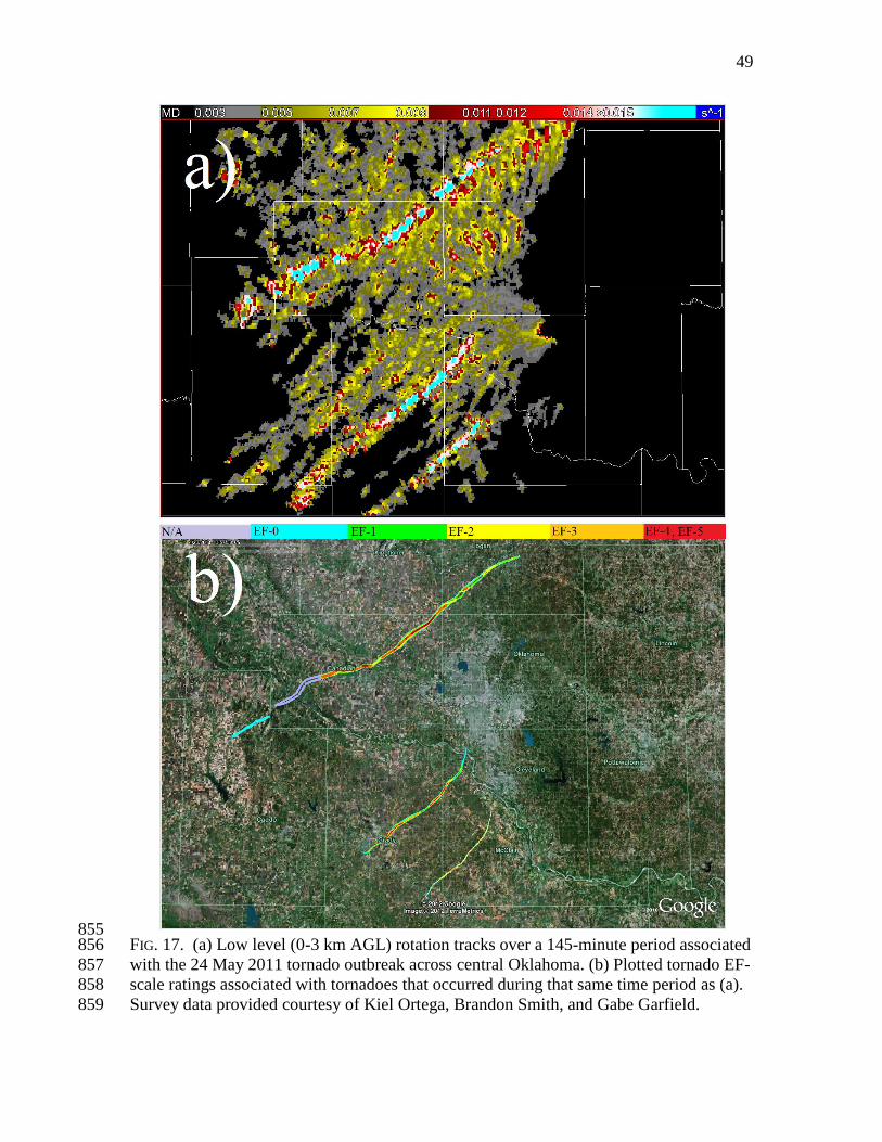
The low level rotation tracks associated with these post-MHT clusters compare well to 433

20
reported tornado tracks in the several cases visually examined. Figure 17 shows how the 434
low level rotation track products associated with tornado damage paths from the 24 May 435
2011 event across central Oklahoma compare to the EF-scale ratings. 436
4. Conclusion 437
NSSL rotation track products are valuable tools in disaster response situations. 438
They allow users to quickly assess both the spatial extent of mesocyclone circulations as 439
seen by radar over time and assess their relative intensities. While these products were 440
useful, a great deal of contamination initially was present due to poor velocity dealiasing, 441
ground clutter, radar test patterns and spurious shear values. These non-meteorological 442
signatures made the tracks nearly impossible to see in some extreme cases. 443
To mitigate these problems for both real-time use and for a multi-year rotation 444
track climatology as part of the MYRORSS project, quality control strategies were 445
developed and implemented. A two-dimensional velocity dealiasing technique using 20-446
km RUC wind data as input made large visual improvements in the quality of the initial 447
radial velocity field. An azimuthal shear range correction algorithm and some simple data 448
thresholds were added to the LLSD shear algorithm. Hysteresis segmentation was used to 449
isolate clusters of high azimuthal shear associated with mesocyclone circulations in each 450
time step of the two-dimensional maximum azimuthal shear fields and MHT techniques 451
were used to associate them throughout time. Any clusters that did not persist for at least 452
10 minutes (2 time steps) or were comprised of an unrealistic distribution of high 453
azimuthal shear values were pruned. The remaining clusters were kept and used to create 454
the rotation track fields. 455

21
While a few issues like the broad shear signatures around some radar sites remain, 456
overall the rotation track fields show a great deal of qualitative improvement after the 457
implementation of the quality control efforts. Whereas the tracks associated with the 458
mesocyclones initially were diluted by background noise and non-meteorological 459
signatures, they are now isolated and easier to interpret. Incorporating these 460
improvements, processing of the MYRORSS rotation track climatology should begin in 461
the near future. 462
Acknowledgments. 463
Funding for the authors was provided under NOAA-OU Cooperative Agreement 464
NA17RJ1227. The authors thank Kiel Ortega, Kevin Manross, John Cintineo, and 465
Jennifer Newman for all their help and advice. The authors also thank Gabe Garfield, 466
Kiel Ortega and Brandon Smith for allowing us to use their damage survey data for the 467
24 May 2011 tornadoes. 468
469
470

22
References 471
Bargen, D. W., and R. C. Brown, 1980: Interactive radar velocity unfolding. Preprints, 472
19th Conf. on Radar Meteorology, Miami, FL, Amer. Meteor. Soc., 278–283. 473
474
Benjamin, S. G., and Coauthors, 2004: An hourly assimilation-forecast cycle: The RUC. 475
Mon. Wea. Rev., 132, 495-518. 476
477
Bergen, W. R., and S. C. Albers, 1988: Two- and three-dimensional de-aliasing of 478
Doppler radar velocities. J. Atmos. Oceanic Technol., 5, 305–319. 479
480
Boren, T. A., J. R. Cruz, and D. S. Zrnić, 1986: An artificial intelligence approach to 481
Doppler weather radar velocity dealiasing., Proc. 23rd Conf. on Radar Meteorology, 482
Snowmass, CO, Amer. Meteor. Soc., 107-110. 483
484
Brown, R. A., L. R. Lemon, and D. W. Burgess, 1978: Tornado detection by pulsed 485
Doppler radar. Mon. Wea. Rev., 106, 29–38. 486
487
Brown, R. A., V. T. Wood, and D. Sirmans, 2002: Improved tornado detection using 488
simulated and actual WSR-88D data with enhanced resolution. J. Atmos. Oceanic 489
Technol., 19, 1759-1771. 490
491
Cintineo, J., T. Smith, V. Lakshmanan, and S. Ansari, 2011: An automated system for 492
processing the Multi-Year Reanalysis of Remotely Sensed Storms (MYRORSS). 493
23
Preprints, 27th Conf. on Interactive Information Processing Systems (IIPS), Seattle, WA, 494
Amer. Meteor. Soc., J9.3. 495
496
Clark, A. J., J. S. Kain, P. T. Marsh, J. Correia, Jr., M. Xue, and F. Kong, 2012: 497
Forecasting tornado path lengths using a 3-dimensional object algorithm applied to 498
convection-allowing forecasts. Wea. Forecasting, In Press. 499
500
Cox, I., and S. L. Hingorani, 1996: An efficient implementation of Reid’s multiple 501
hypothesis tracking algorithm and its evaluation for the purpose of visual tracking. IEEE 502
Trans. Pattern Anal. Mach. Intell., 18, 138-150. 503
504
Crum, T. D., and R. K. Alberty, 1993: The WSR-88D and the WSR-88D Operational 505
Support Facility. Bull. Amer. Meteor. Soc., 74, 1669-1687. 506
507
Eilts, M. D., and S. D. Smith, 1990: Efficient dealiasing of Doppler velocities using local 508
environment constraints. J. Atmos. Oceanic Technol., 7, 118–128. 509
510
Elmore, K. M., E. D. Albo, R. K. Goodrich, and D. J. Peters, 1994: NASA/NCAR 511
airborne and ground-based wind shear studies. Final Report, contract no. NCC1-155, 343 512
pp. 513
514
Forbes, G. S., 1981: On the reliability of hook echoes as tornado indicators. Mon. Wea. 515
Rev., 109, 1457–1466. 516

24
517
Fulton, R., D. Breidenback, D. Miller, and T. O’Bannon, 1998: The WSR-88D rainfall 518
algorithm. Wea. Forecasting, 13, 377-395. 519
520
Jain, A., 1989: Fundamentals of Digital Image Processing. Prentice Hall, 569 pp. 521
522
Jing, Z., and G. Wiener, 1993: Two-dimensional dealiasing of Doppler velocities. J. 523
Atmos. Oceanic Technol., 10, 798–808. 524
525
Kain, J. S., S. R. Dembek, S. J. Weiss, J. L. Case, J. J. Levit, R. A. Sobash, 2010: 526
Extracting unique information from high-resolution forecast models: Monitoring selected 527
fields and phenomena every time step. Wea. Forecasting, 25, 1536–1542. 528
529
Kessinger, C., S. Ellis, and J. Van Andel, 2003: The radar echo classifier: A fuzzy logic 530
algorithm for the WSR-88D. Pre-prints, Third Conf. on Artificial Applications to the 531
Environmental Sciences, Long Beach, CA, Amer. Meteor. Soc., CD-ROM, P1.6. 532
533
Lakshmanan, V., R. Rabin, and V. DeBrunner, 2003: Multiscale storm identification and 534
forecast. J. Atmos. Res., 367-380. 535
536
Lakshmanan, V., T. Smith, K. Hondl, G. J. Stumpf and A. Witt, 2006: A real-time, three-537
dimensional, rapidly updating, heterogeneous radar merger technique for reflectivity, 538
velocity and derived products. Wea. Forecasting, 21, 802-823. 539

25
540
Lakshmanan, V., A. Fritz, T. Smith, K. Hondl, and G. J. Stumpf, 2007a: An automated 541
technique to quality control radar reflectivity data. J. Appl. Meteor., 46, 288-305. 542
543
Lakshmanan, V., T. Smith, G. J. Stumpf, and K. Hondl, 2007b: The Warning Decision 544
Support System – Integrated Information. Wea. Forecasting, 22, 596-612. 545
546
Lakshmanan, V., J. Zhang, and K. Howard, 2010: A technique to censor biological 547
echoes in radar reflectivity data. J. Appl. Meteor., 49, 35-462. 548
549
Lakshmanan, V., 2012: Neighborhood and window operations. Automating the Analysis 550
of Spatial Grids: A Practical Guide to Data Mining Geospatial Images for Human & 551
Environmental Applications, Springer, 129-171. 552
553
Lakshmanan, V., M. Miller, and T. Smith, 2012: Quality control of accumulated fields by 554
applying spatial and temporal constraints. J. Atmos. Ocean. Tech., Accepted. [Available 555
online at http://www.cimms.ou.edu/~lakshman/Papers/mhtqc.pdf.] 556
557
Liu, S., M. Xue, and Q. Xu, 2007: Using wavelet analysis to detect tornadoes from 558
Doppler radar radial-velocity observations. J. Atmos. Oceanic Technol., 24, 344-359. 559
560
Merritt, M. W., 1984: Automatic velocity dealiasing for real-time applications. Proc. 561
22nd Conf. on Radar Meteorology, Zurich, Amer. Meteor. Soc., 528-533. 562

26
Mitchell, E. D., and K. L. Elmore, 1998: A technique for identifying regions of high 563
shear associated with mesocyclones and tornadic vortex signatures. Preprints, 14th 564
International Conference on Interactive Information and Processing Systems (IIPS) for 565
Meteorology, Oceanography, and Hydrology, Phoenix, AZ. Amer. Meteor. Soc., 312-566
315. 567
568
Mitchell, E. D., S. V. Vasiloff, G. J. Stumpf, A. Witt, M. D. Eilts, J. T. Johnson, K. W. 569
Thomas, 1998: The National Severe Storms Laboratory tornado detection algorithm. 570
Wea. Forecasting, 13, 352–366. 571
572
Murty, K. G., 1968: An algorithm for ranking all the assignments in order of increasing 573
cost. Operations Research, 16, 682-687. 574
575
Newman, J. F., V. Lakshmanan, P. L. Heinselman, M. B. Richman, and T. M. Smith, 576
2011: Range-correcting azimuthal shear in Doppler radar data. Wea. Forecasting, In 577
Press. 578
579
National Oceanic and Atmospheric Administration (NOAA) National Severe Storms 580
Laboratory (NSSL), cited 2011: NOAA technology helps American Red Cross respond 581
faster. [Available online at https://secure.nssl.noaa.gov/briefings/2011/06/noaa-582
technology-helps-american-red-cross-respond-faster/] 583
584

27
Ray, P. S., and C. Ziegler, 1977: De-aliasing first-moment Doppler estimates. J. Appl. 585
Meteor., 16, 563–564. 586
587
Root, B., M. Yeary, and T.-Y. Yu, 2011: Novel storm cell tracking with multiple 588
hypothesis tracking. Preprints, 27th Conf. on Interactive Information Processing Systems 589
(IIPS), Seattle, WA, Amer. Meteor. Soc., 8B.3. 590
591
Steiner, M., and J. A. Smith, 2002: Use of three-dimensional reflectivity structure for 592
automated detection and removal of nonprecipitating echoes in radar data. J. Atmos. 593
Oceanic Technol., 19, 673–686. 594
595
Stumpf, G. J., A. Witt, E. D. Mitchell, P. L. Spencer, J. T. Johnson, M. D. Eilts, K. W. 596
Thomas, and D. W. Burgess, 1998: The National Severe Storms Laboratory mesocyclone 597
detection algorithm for the WSR-88D. Wea. Forecasting, 13, 304-326. 598
599
Smith, T. M., and K. L. Elmore, 2004: The use of radial velocity derivatives to diagnose 600
rotation and divergence. Preprints, 11th Conf.on Aviation, Range and Aerospace, 601
Hyannis, MA, Amer. Meteor. Soc., P5.6. 602
603
Wood, V. T., and R. A. Brown, 1997: Effects of radar sampling on single-Doppler 604
velocity signatures of mesocyclones and tornadoes. Wea. Forecasting, 12, 928–938. 605
606
607

28
List of Figures 608
FIG. 1. Low level (0-3 km AGL) rotation tracks from the 27 April 2011 tornado outbreak. 609
Swaths of high maximum azimuthal shear approximate the movement and strength of 610
mesocyclone circulations within the supercells that moved southwest to northeast across 611
the states of Alabama, Mississippi, and Tennessee between 16 UTC on 27 April and 00 612
UTC on 28 April. 613
614
FIG. 2. Low level (0-3 km AGL) rotation tracks across Virginia, North Carolina and 615
South Carolina from the 16 April 2011 tornado outbreak generated using the default 616
WSR-88D velocity dealiasing technique and without any quality control techniques. The 617
spikes of high azimuthal shear values are caused by poor velocity dealiasing along radials 618
and can make data interpretation difficult, if not impossible, in some areas. 619
620
FIG. 3. Radial velocity fields and the corresponding azimuthal shear fields from KDGX 621
on 27 April 2011 at 2151 UTC created using different dealiasing strategies. (a) Radial 622
velocity dealiased using the LED algorithm. (b) Azimuthal shear field associated with (a). 623
(c) Radial velocity dealiased using the LED algorithm with an environmental wind field 624
from an input 20-km RUC point sounding. (d) Azimuthal shear associated with (c). (e) 625
Radial velocity field dealiased using the Jing and Weiner (1993) technique with an 626
environmental wind field from an input 20-km RUC point sounding. (f) Azimuthal shear 627
field associated with (e). 628
629
630

29
FIG. 4. Flow chart showing how rotation track products are created. Grey boxes with 631
dashed lines represent algorithms and white boxes with solid lines represent data fields. 632
633
FIG. 5. (a) Low level (0-3 km AGL) rotation track field from the 2 March 2012 outbreak 634
from the KVWX radar site before data removal near the radar site. Note the high values 635
of azimuthal shear surrounding the radar site at the center of the image. (b) The same 636
rotation track field after the removal of data within a 5-km radius of the radar site. This 637
removal will only be performed for the climatology, not in real-time. 638
639
FIG. 6. (a) Reflectivity, (b) ReflectivityQC, (c) radial velocity, and (d) azimuthal shear 640
fields associated with a supercell over central Alabama on 27 April 2011 at 2107 UTC. 641
642
FIG. 7. A schematic showing how hysteresis segmentation works. The first and last 643
peaks of azimuthal shear values will be associated with clusters, while the middle peak 644
will not be associated with a cluster because it contains no values above the higher data 645
threshold. 646
647
FIG. 8. Low level (0-3 km AGL) rotation tracks associated with the tornadic supercells 648
that moved across Mississippi and Alabama between 16 UTC on 27 April 2011 and 00 649
UTC on 28 April 2011. (a) Rotation tracks before hysteresis segmentation. (b) Rotation 650
tracks after hysteresis segmentation is used to threshold the field. 651
652

30
FIG. 9. Example of how the MHT algorithm tracks clusters and generates hypotheses. 653
Solid shapes represent the position of azimuthal shear clusters at the given time step. 654
Solid arrows show the movement of clusters between time steps. Dotted shapes show the 655
projected locations of the azimuthal shear clusters in the next time steps. Dashed arrows 656
show the projected movement of the clusters between time steps. Shape A shows the 657
projected location of the original cluster at time t. Shape B represents the actual location 658
of the original cluster at time t. The algorithm generates two hypotheses for time t + 1 (C 659
and D). If the location of B is an error, then at time t + 1 the cluster should move to 660
position D. If the location of B is not an error but a change in motion, then B should 661
move to location C at time t + 1. At time t + 1, the discovery of the target at either C or D 662
will confirm one hypothesis and disprove the other. The disproved cluster is deleted and 663
the confirmed one continues on to the next time step. In this case, given the strange shape 664
and size of B, it is likely that this cluster is associated with a non-meteorological shear 665
signature and will not persist in time t + 1. 666
667
FIG. 10. Multiple hypothesis tracking flow chart adapted from Root et al. (2011). 668
669
FIG. 11. An example of a cluster of high azimuthal shear values associated with a 670
mesocyclone circulation is shown in (a) and the histogram of its data values after 671
hysteresis segmentation is shown in (b). An example of a cluster of high azimuthal shear 672
values associated with a non-meteorological artifact is shown in (c) and the histogram of 673
its data values after hysteresis segmentation is shown in (d). Note the nearly uniform 674
distribution of very high values. 675

31
676
FIG. 12. Low level (0-3 km AGL) rotation tracks associated the 27 April 2011 tornado 677
outbreak across Mississippi and Alabama produced using different velocity dealiasing 678
techniques, no thresholds and no MHT. (a) Tracks made using velocity dealiased with 679
the LED algorithm. (b) Tracks made using velocity dealiased with the LED algorithm 680
with 20-km RUC input sounding. (c) Tracks made using velocity dealiased with the Jing 681
and Weiner (1993) technique. (d) Tracks made using velocity dealiased with the Jing and 682
Weiner (1993) technique with 20-km RUC input sounding. 683
684
FIG. 13. Low level (0-3 km AGL) rotation tracks from the 27 April 2011 tornado 685
outbreak. (a) Tracks created using the Jing and Weiner (1993) velocity dealiasing 686
method with the input 20-km RUC sounding, without the azimuthal shear range 687
correction and without the increased ReflectivityQC threshold. (b) Tracks created using 688
the same velocity dealiasing method as in (a), but with the azimuthal shear range 689
correction and the increased ReflectivityQC threshold. Note that the circled area of high 690
azimuthal shear values associated with dealiasing errors over central Tennessee is much 691
less prominent in (b). 692
693
FIG. 14. Low level (0-3 km AGL) rotation track from the 27 April 2011 tornado 694
outbreak. (a) Tracks created using the Jing and Weiner (1993) velocity dealiasing 695
method with the input 20-km RUC sounding, with range correction, increased 696
ReflectivityQC thresholds and without hysteresis segmentation. (b) The same tracks as 697
(a) but with hysteresis segmentation implemented. 698

32
699
FIG. 15. Low level (0-3 km AGL) rotation tracks across Mississippi and Alabama from 700
the 27 April 2011 tornado outbreak. (a) Tracks created using the Jing and Weiner (1993) 701
velocity dealiasing method with the input 20-km RUC sounding, with range correction, 702
increased ReflectivityQC thresholds, hysteresis segmentation and without MHT. (b) The 703
same tracks as (a) but with MHT. Note the several small clusters in west-central 704
Mississippi are removed. 705
706
FIG. 16. The impacts of the quality control efforts on low level (0-3 km AGL) rotation 707
track products associated with four recent tornado events: the 27 April 2011 event before 708
(a) and after (b) quality control, the 16 April 2011 event before (c) and after (d) quality 709
control, the 24 May 2011 event before (e) and after (f) quality control, and the 2 March 710
2012 event before (g) and after (h) quality control. 711
712
FIG. 17. (a) Low level (0-3 km AGL) rotation tracks over a 145-minute period associated 713
with the 24 May 2011 tornado outbreak across central Oklahoma. (b) Plotted tornado EF-714
scale ratings associated with tornadoes that occurred during that same time period as (a). 715
Survey data provided courtesy of Kiel Ortega, Brandon Smith, and Gabe Garfield. 716
717

33
718 719
FIG. 1. Low level (0-3 km AGL) rotation tracks from the 27 April 2011 tornado outbreak. 720
Swaths of high maximum azimuthal shear approximate the movement and strength of 721
mesocyclone circulations within the supercells that moved southwest to northeast across 722
the states of Alabama, Mississippi, and Tennessee between 16 UTC on 27 April and 00 723
UTC on 28 April. 724
725

34
726
FIG. 2. Low level (0-3 km AGL) rotation tracks across Virginia, North Carolina and 727
South Carolina from the 16 April 2011 tornado outbreak generated using the default 728
WSR-88D velocity dealiasing technique and without any quality control techniques. The 729
spikes of high azimuthal shear values are caused by poor velocity dealiasing along radials 730
and can make data interpretation difficult, if not impossible, in some areas. 731
732

35
733 FIG. 3. Radial velocity fields and the corresponding azimuthal shear fields from KDGX 734
on 27 April 2011 at 2151 UTC created using different dealiasing strategies. (a) Radial 735
velocity dealiased using the LED algorithm. (b) Azimuthal shear field associated with (a). 736
(c) Radial velocity dealiased using the LED algorithm with an environmental wind field 737
from an input 20-km RUC point sounding. (d) Azimuthal shear associated with (c). (e) 738
Radial velocity field dealiased using the Jing and Weiner (1993) technique with an 739
environmental wind field from an input 20-km RUC point sounding. (f) Azimuthal shear 740
field associated with (e). 741

36
742
743
FIG. 4. Flow chart showing how rotation track products are created. Grey boxes with 744
dashed lines represent algorithms and white boxes with solid lines represent data fields. 745
746

37
747 FIG. 5. (a) Low level (0-3 km AGL) rotation track field from the 2 March 2012 748
outbreak from the KVWX radar site before data removal near the radar site. Note the 749
high values of azimuthal shear surrounding the radar site at the center of the image. (b) 750
The same rotation track field after the removal of data within a 5-km radius of the radar 751
site. This removal will only be performed for the climatology, not in real-time. 752

38
753 FIG. 6. (a) Reflectivity, (b) ReflectivityQC, (c) radial velocity, and (d) azimuthal shear 754
fields associated with a supercell over central Alabama on 27 April 2011 at 2107 UTC. 755
756
757
758
759
760
761
762
763
764
39
765 766
FIG. 7. A schematic showing how hysteresis segmentation works. The first and last peaks 767
of azimuthal shear values will be associated with clusters, while the middle peak will not 768
be associated with a cluster because it contains no values above the higher data threshold. 769
770
771
772
773

40
774 FIG. 8. Low level (0-3 km AGL) rotation tracks associated with the tornadic supercells 775
that moved across Mississippi and Alabama between 16 UTC on 27 April 2011 and 00 776
UTC on 28 April 2011. (a) Rotation tracks before hysteresis segmentation. (b) Rotation 777
tracks after hysteresis segmentation is used to threshold the field. 778

41
779 780
FIG. 9. Example of how the MHT algorithm tracks clusters and generates hypotheses. 781
Solid shapes represent the position of azimuthal shear clusters at the given time step. 782
Solid arrows show the movement of clusters between time steps. Dotted shapes show the 783
projected locations of the azimuthal shear clusters in the next time steps. Dashed arrows 784
show the projected movement of the clusters between time steps. Shape A shows the 785
projected location of the original cluster at time t. Shape B represents the actual location 786
of the original cluster at time t. The algorithm generates two hypotheses for time t + 1 (C 787
and D). If the location of B is an error, then at time t + 1 the cluster should move to 788
position D. If the location of B is not an error but a change in motion, then B should 789
move to location C at time t + 1. At time t + 1, the discovery of the target at either C or D 790
will confirm one hypothesis and disprove the other. The disproved cluster is deleted and 791
the confirmed one continues on to the next time step. In this case, given the strange shape 792
and size of B, it is likely that this cluster is associated with a non-meteorological shear 793
signature and will not persist in time t + 1. 794
795
796
b)
a)

42
797 798
FIG. 10. Multiple hypothesis tracking flow chart adapted from Root et al. (2011). 799
800

43
801
FIG. 11. An example of a cluster of high azimuthal shear values associated with a 802
mesocyclone circulation is shown in (a) and the histogram of its data values after 803
hysteresis segmentation is shown in (b). An example of a cluster of high azimuthal shear 804
values associated with a non-meteorological artifact is shown in (c) and the histogram of 805
its data values after hysteresis segmentation is shown in (d). Note the nearly uniform 806
distribution of very high values. 807
808
809
810

44
811 FIG. 12. Low level (0-3 km AGL) rotation tracks associated the 27 April 2011 tornado 812
outbreak across Mississippi and Alabama produced using different velocity dealiasing 813
techniques, no thresholds and no MHT. (a) Tracks made using velocity dealiased with 814
the LED algorithm. (b) Tracks made using velocity dealiased with the LED algorithm 815
with 20-km RUC input sounding. (c) Tracks made using velocity dealiased with the Jing 816
and Weiner (1993) technique. (d) Tracks made using velocity dealiased with the Jing and 817
Weiner (1993) technique with 20-km RUC input sounding. 818
819
820

45
821 822
FIG. 13. Low level (0-3 km AGL) rotation tracks from the 27 April 2011 tornado 823
outbreak. (a) Tracks created using the Jing and Weiner (1993) velocity dealiasing 824
method with the input 20-km RUC sounding, without the azimuthal shear range 825
correction and without the increased ReflectivityQC threshold. (b) Tracks created using 826
the same velocity dealiasing method as in (a), but with the azimuthal shear range 827
correction and the increased ReflectivityQC threshold. Note that the circled area of high 828
azimuthal shear values associated with dealiasing errors over central Tennessee is much 829
less prominent in (b). 830
46
831 832
FIG. 14. Low level (0-3 km AGL) rotation track from the 27 April 2011 tornado 833
outbreak. (a) Tracks created using the Jing and Weiner (1993) velocity dealiasing 834
method with the input 20-km RUC sounding, with range correction, increased 835
ReflectivityQC thresholds and without hysteresis segmentation. (b) The same tracks as 836
(a) but with hysteresis segmentation implemented. 837
838

47
839 840
FIG. 15. Low level (0-3km AGL) rotation tracks across Mississippi and Alabama from 841
the 27 April 2011 tornado outbreak. (a) Tracks created using the Jing and Weiner (1993) 842
velocity dealiasing method with the input 20-km RUC sounding, with range correction, 843
increased ReflectivityQC thresholds, hysteresis segmentation and without MHT. (b) The 844
same tracks as (a) but with MHT. Note the several small clusters in west-central 845
Mississippi are removed. 846
847
848

48
849 FIG. 16. The impacts of the quality control efforts on low level (0-3 km AGL) rotation 850
track products associated with four recent tornado events: the 27 April 2011 event before 851
(a) and after (b) quality control, the 16 April 2011 event before (c) and after (d) quality 852
control, the 24 May 2011 event before (e) and after (f) quality control, and the 2 March 853
2012 event before (g) and after (h) quality control. 854
49
855 FIG. 17. (a) Low level (0-3 km AGL) rotation tracks over a 145-minute period associated 856
with the 24 May 2011 tornado outbreak across central Oklahoma. (b) Plotted tornado EF-857
scale ratings associated with tornadoes that occurred during that same time period as (a). 858
Survey data provided courtesy of Kiel Ortega, Brandon Smith, and Gabe Garfield. 859