Embed Size (px)
Citation preview

Sampling Strategies for Tornado and Mesocyclone Detection Using DynamicallyAdaptive Doppler Radars: A Simulation Study
JESSICA L. PROUD* AND KELVIN K. DROEGEMEIER
Center for Analysis and Prediction of Storms, and School of Meteorology, University of Oklahoma, Norman, Oklahoma
VINCENT T. WOOD AND RODGER A. BROWN
NOAA/National Severe Storms Laboratory, Norman, Oklahoma
(Manuscript received 29 October 2007, in final form 25 July 2008)
ABSTRACT
Increasing tornado and severe storm warning lead time (lead time is defined here as the elapsed time
between the issuance of a watch or warning and the time at which the anticipated weather event first impacts
the specified region) through the use of radar observations has long been a challenge for researchers and
operational forecasters. To improve lead time and the probability of detecting tornadoes while decreasing
the false alarm ratio, a greater understanding, obtained in part by more complete observations, is needed
about the region of storms within which tornadoes form and persist. Driven in large part by this need, but also
by the goal of using numerical models to explicitly predict intense local weather such as thunderstorms, the
National Science Foundation established, in fall 2003, the Engineering Research Center for Collaborative
Adaptive Sensing of the Atmosphere (CASA). CASA is developing a revolutionary new paradigm of using a
network of small, closely spaced, inexpensive, low-power dual-polarization Doppler weather radars to
overcome the inability of widely spaced, high-power radars to sample large regions of the lower atmosphere
owing to the curvature of earth given that zero or negative beam elevation angles are not allowed. Also,
current radar technology operates mostly independently of the weather and end-user needs, thus producing
valuable information on storms as a whole but not focused on any specific phenomenon or need. Conversely,
CASA utilizes a dynamically adaptive sensing paradigm to identify, and optimally sample, multiple targets
based upon their observed characteristics in order to meet a variety of often competing end-user needs.
The goal of this study is to evaluate a variety of adaptive sampling strategies for CASA radars to assess
their effectiveness in identifying intense low-altitude vortices. Such identification, for the purposes of this
study, is defined as achieving a best fit of simulated observations to an analytic model of a tornado or
mesocyclone. Several parameters are varied in this study including the size of the vortex, azimuthal sampling
interval, distance of the vortex from the radar, and radar beamwidth.
Results show that, in the case of small vortices, adaptively decreasing the azimuthal sampling interval (i.e.,
overlapping beams) is beneficial in comparison to conventional azimuthal sampling that is approximately
equal to the beamwidth. However, the benefit is limited to factors of 2 in overlapping. When simulating the
performance of a CASA radar in comparison to that of a Weather Surveillance Radar-1988 Doppler (WSR-
88D) at close range, with both operating in the conventional nonoverlapping mode, the WSR-88D (with a
beamwidth about half that of a CASA radar) performs better. However, when overlapping is applied to the
CASA radar, for which little additional processing time is required, the results are comparable. In effect, the
sampling resolution of a radar can be increased simply by decreasing the azimuthal sampling interval as
opposed to installing a larger antenna.
1. Introduction
The current National Weather Service (NWS)
Weather Surveillance Radar-1988 Doppler (WSR-88D;
Crum and Alberty 1993) radar network is the principal
tool used for detecting severe storms and tornadoes and
for issuing warnings. This network has been critical
to the forecasting of severe weather and has saved
* Current affiliation: Renaissance Computing Institute, Chapel
Hill, North Carolina.
Corresponding author address: Jessica L. Proud, Renaissance
Computing Institute, 100 Europa Drive, Suite 540, Chapel Hill,
NC 27517.
E-mail: [email protected]
492 J O U R N A L O F A T M O S P H E R I C A N D O C E A N I C T E C H N O L O G Y VOLUME 26
DOI: 10.1175/2008JTECHA1087.1
� 2009 American Meteorological Society

countless lives since its formal commissioning in 1994
(Simmons and Sutter 2005). To improve lead time and
the probability of detecting tornadoes while decreasing
false alarms (Fig. 1), a greater understanding, obtained
in part by more complete observations, is needed
about the region of storms within which tornadoes
form and persist; that is, the region within a few kilo-
meters of the ground. Driven in large part by this need,
but also by the goal of using numerical models to ex-
plicitly predict intense local weather such as thunder-
storms, the National Science Foundation (NSF) es-
tablished in fall 2003 the Engineering Research Center
for Collaborative Adaptive Sensing of the Atmosphere
(CASA).
CASA is led by the University of Massachusetts at
Amherst with several academic partners, including the
University of Oklahoma, Colorado State University,
and the University of Puerto Rico at Mayaguez, along
with industrial, educational, and end-user partners. It
is developing five radar test beds, the first of which is
located in southwestern Oklahoma and consists of four
radars and emphasizes the detection of storms and
tornadoes. This test bed collected numerous datasets
during the spring 2007 and 2008 severe weather sea-
sons, and the data now are being analyzed (e.g., Kong
et al. 2007; Weiss et al. 2007; Kain et al. 2009). The
second test bed, which is being developed in downtown
Houston, emphasizes quantitative precipitation esti-
mation for hydrology. Located in Puerto Rico, the
third test bed is being developed entirely by students
and utilizes solar power and wireless communication
technologies to study quantitative precipitation estima-
tion and forecasts in mountainous terrain. The fourth
and fifth test beds focus, respectively, on clear-air sens-
ing and phased array technology, and are now being
planned.
In contrast to most current weather radars, which
operate in a ‘‘sit and spin’’ mode independent of evolving
weather,1 CASA radars are designed to operate in a
distributed, collaborative, adaptive framework (DCAS;
McLaughlin et al. 2005). ‘‘Distributed’’ refers to placing
radars in clusters with a spacing much closer (;25 km)
than that of the WSR-88D network so as to overcome
sampling problems (e.g., azimuthal resolution degra-
dation or beam location above ground) that occur at a
long range owing to beam spreading and the earth’s
curvature. ‘‘Collaborative’’ connotes the coordinated
targeting of multiple radar beams based on atmospheric
and hydrologic analysis tools, such as detection, pre-
dicting, and tracking algorithms (McLaughlin et al.
2005). By utilizing this collaboration, the system allo-
cates resources such as radiated power, beam position,
and polarization diversity for optimally sampling re-
gions of the atmosphere where a particular threat exists.
The term ‘‘adaptive’’ refers to the ability of the CASA
radars and the associated infrastructure to quickly re-
configure (e.g., begin using a smaller azimuthal sam-
pling interval) in response to changing weather and to
meet various end-user needs.
Another unique adaptive characteristic of CASA ra-
dars is the ability to change from sampling a large area
to much smaller sector scans, say of a tornadic region,
independently or collaboratively with other CASA ra-
dars. In contrast, WSR-88D radars scan independently
of one other and continuously surveil the entire volume
largely independent of weather occurring within it.
Given these features, a fundamental research challenge
for CASA concerns understanding which modes of ra-
dar operation will yield the maximum amount of useful
information about a particular weather phenomenon
while minimizing the use of available resources (so they
are available for other phenomena or use by other
neighboring radars).
As a first step toward addressing this and related
challenges, the goal of the present study is to use
pseudo-observations of an idealized vertical vortex to
evaluate a variety of sampling strategies for CASA ra-
dars in order to determine which might be most effec-
tive for real tornadoes and mesocyclones. Here, effec-
tiveness isdefinedas thebestfitof thepseudo-observations
to an analytic model of tornadoes and mesocyclones.
FIG. 1. Shown here is the probability of detection, false alarm
ratio, and lead time of tornado warnings from 1986 to 2006.
(B. MacAloney Jr., National Weather Service, 2007, personal
communication). Installation of WSR-88Ds took place during
1992–96.
1 The Terminal Doppler Weather Radar (TDWR; e.g., Wieler
and Shrader 1991), operates in a sector scan mode to detect mi-
crobursts and other aviation hazards. The WSR-88D utilizes a
variety of volume coverage patterns (e.g., Klazura and Imy 1993;
Brown et al. 2005) that are chosen based upon weather charac-
teristics; however, none involve sector scanning or other modes of
adaptation to specific weather features.
MARCH 2009 P R O U D E T A L . 493

Several parameters are tested, including the radius of the
vortex, azimuthal sampling interval, and the distance of
the vortex center from the radar. It may seem logical to
sample a vortex or other atmospheric phenomena with
as much spatial and temporal resolution as possible, but
doing so may actually waste available radar resources2
while providing no useful added information.
The allocation of resources is especially important in
DCAS, where multiple, frequently competing end-user
goals must be met in an optimal manner. In the current
radar test bed located in Oklahoma, this allocation is
performed via a policy mediation framework in which
detection algorithms run in real time on radar moment
data categorize observed signatures and store their at-
tributes (e.g., feature type, time of development, loca-
tion) in a so-called feature repository. This information
is combined with user-specified priorities (Philips et al.
2007) to produce scanning pattern commands that are
communicated to the radars by the Meteorological
Command and Control (MC&C) system. The frequency
of this communication is determined by the radar
‘‘heartbeat,’’ which presently is 60 s. That is, every 60 s,
the radars can be retasked to scan different regions at
different rates. For more information on CASA scanning
strategies, see Brotzge et al. (2005, 2008), and Gagne
et al. (2008). The results of the present study are expected
to help optimize this process for identifying potentially
hazardous atmospheric vortices early in their lifetime.
Section 2 describes the methodology used, including a
detailed explanation of the vortex model, radar emu-
lator, and retrieval technique, along with parameters
varied to study various sampling strategies. The results
are discussed in section 3, and a summary and sugges-
tions for future work are presented in section 4.
2. Methodology
a. Vortex model
To create a representative tornadic or mesocyclonic
flow field appropriate for sampling by a virtual CASA
radar, an analytic vortex model is used to generate an
idealized one-dimensional (horizontally through the cen-
ter of the vortex) azimuthal velocity profile. An analytic
vortex model, for which an exact solution is available, is
appropriate for use in assessing the potential value of
various adaptive strategies prior to their application
with real data. One familiar model is the Rankine (1901,
574–578) combined vortex (RCV), which is given by
vt 5 Vxf ðr, RxÞ, (1)
where vt is the tangential velocity, Vx is the maximum
tangential velocity, and f(r,Rx) is the dimensionless ve-
locity profile given by
f ðr, RxÞ5
r
Rx, 0 # r , Rx
Rx
r, Rx # r
.
8><>: (2)
Here, r is the radial distance from the vortex center and
Rx is the core radius at which Vx occurs. The ‘‘core’’ of
the vortex (r # Rx) is characterized by solid body ro-
tation, while for r $ Rx, potential flow is assumed.
The RCV profile was not used in the present work
owing to the discontinuity in velocity at r 5 Rx and its
effects on the minimization algorithm used here. The
observed Doppler core radius is usually larger than Rx
(which needs to be known to make an initial guess)
because of smearing effects within the radar beam.
When applying the minimization algorithm, an updated
Rx must be known before the velocity profile is scanned
again, and it is difficult for the algorithm to determine
which part of the velocity profile (core or potential flow)
the radar is sampling. This can cause instability in the
algorithm and a lack of convergence to a solution. Also,
according to high-resolution tornado observations (e.g.,
Wurman and Gill 2000), this discontinuity does not exist
in real tornadoes, and the decay of tangential wind
speed with distance outside the core of solid body ro-
tation occurs less rapidly than with the RCV.
For this reason, we use a more flexible analytic model
(developed by L. White, University of Oklahoma, per-
sonal communication 2005) that does not contain a
discontinuity and that decays more slowly than the
RCV. Referred to as the three-parameter vortex model
(TPVM), it is characterized by a function that has no
discontinuities yet retains the principal features of and
provides greater flexibility than the RCV:3
Vnðr, RxÞ5 VxFn, (3)
where Fn 5 2nR2n�1x r/½ð2n� 1ÞR2n
x 1 r2n� is the velocity
profile of the vortex, Vx is tangential velocity, r the ra-
dius from the vortex center, and n is a nonzero integer
value that controls the velocity profile beyond the core
radius. After testing various combinations of (3) with
2 Note that maximizing resources, in a framework such as
CASA in real time, is inherently a property of dynamically adap-
tive systems.
3 Unlike the RCV, the TPVM does not conserve angular mo-
mentum. However, that property is unimportant for the purposes
of this study.
494 J O U R N A L O F A T M O S P H E R I C A N D O C E A N I C T E C H N O L O G Y VOLUME 26
different values of n, three different tangential velocity
profiles were selected for this study:
V1ðr, RxÞ5 Vx2rRx
R2x 1 r2
!, (4a)
V2ðr, RxÞ5 Vx4rR3
x
3R4x 1 r4
!, and (4b)
V12ðr, RxÞ51
2V1ðr, RxÞ1 V2ðr, RxÞ½ �
5 VxRxr
R2x 1 r2
12R3
xr
3R4x 1 r4
!. (4c)
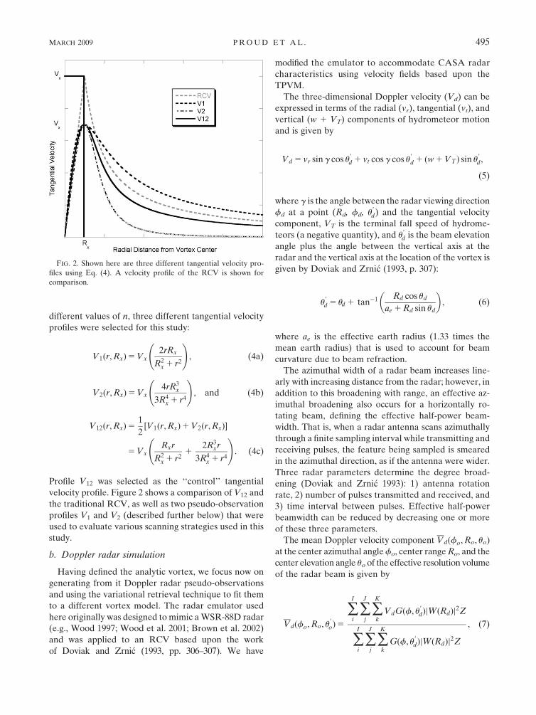
Profile V12 was selected as the ‘‘control’’ tangential
velocity profile. Figure 2 shows a comparison of V12 and
the traditional RCV, as well as two pseudo-observation
profiles V1 and V2 (described further below) that were
used to evaluate various scanning strategies used in this
study.
b. Doppler radar simulation
Having defined the analytic vortex, we focus now on
generating from it Doppler radar pseudo-observations
and using the variational retrieval technique to fit them
to a different vortex model. The radar emulator used
here originally was designed to mimic a WSR-88D radar
(e.g., Wood 1997; Wood et al. 2001; Brown et al. 2002)
and was applied to an RCV based upon the work
of Doviak and Zrni�c (1993, pp. 306–307). We have
modified the emulator to accommodate CASA radar
characteristics using velocity fields based upon the
TPVM.
The three-dimensional Doppler velocity (Vd) can be
expressed in terms of the radial (vr), tangential (vt), and
vertical (w 1 VT) components of hydrometeor motion
and is given by
Vd 5 vr sin g cos u9d 1 vt cos g cos u9
d 1 ðw 1 VT Þ sin u9d,
(5)
where g is the angle between the radar viewing direction
fd at a point (Rd, fd, u9d) and the tangential velocity
component, VT is the terminal fall speed of hydrome-
teors (a negative quantity), and u9d is the beam elevation
angle plus the angle between the vertical axis at the
radar and the vertical axis at the location of the vortex is
given by Doviak and Zrni�c (1993, p. 307):
u9d 5 ud 1 tan�1 Rd cos ud
ae 1 Rd sin ud
� �, (6)
where ae is the effective earth radius (1.33 times the
mean earth radius) that is used to account for beam
curvature due to beam refraction.
The azimuthal width of a radar beam increases line-
arly with increasing distance from the radar; however, in
addition to this broadening with range, an effective az-
imuthal broadening also occurs for a horizontally ro-
tating beam, defining the effective half-power beam-
width. That is, when a radar antenna scans azimuthally
through a finite sampling interval while transmitting and
receiving pulses, the feature being sampled is smeared
in the azimuthal direction, as if the antenna were wider.
Three radar parameters determine the degree broad-
ening (Doviak and Zrni�c 1993): 1) antenna rotation
rate, 2) number of pulses transmitted and received, and
3) time interval between pulses. Effective half-power
beamwidth can be reduced by decreasing one or more
of these three parameters.
The mean Doppler velocity component Vdðfo, Ro, uoÞ
at the center azimuthal angle fo, center range Ro, and the
center elevation angle uo of the effective resolution volume
of the radar beam is given by
Vdðfo, Ro, u9oÞ5
�I
i�
J
j�K
kVdGðf, u9
dÞjWðRdÞj2Z
�I
i�
J
j�K
kGðf, u9
dÞjWðRdÞj2Z
, (7)
FIG. 2. Shown here are three different tangential velocity pro-
files using Eq. (4). A velocity profile of the RCV is shown for
comparison.
MARCH 2009 P R O U D E T A L . 495

where i, j, k are the azimuth, range, and elevation di-
rections, respectively; f is the azimuthal angle; and u is
the elevation angle. Reflectivity (Z) is assumed uniform
across the vortex; G(f, u9d) is the two-way Gaussian
pattern weighting function used to weight Doppler ve-
locity at the (fi, uk) data point and is given by
Gðf, u9dÞ5 exp �
ðfi � foÞ2
2s 2f
�ðu9
k � u9oÞ
2
2s 2u
" #. (8)
In (8), sf2 and su
2 are the standard deviations of the
Gaussian density in the f and u directions, respectively,
and are specified by
s2f 5
f2e
16 ln 2, (9)
s2u 5
u 21
16 ln 2, (10)
where fe is the effective half-power beamwidth in the
azimuthal direction and u1 is the vertical half-power
beamwidth in the elevation direction. Another term in
(7) is the Gaussian-shaped range weighting function,
jWðRdÞj2, used to weight Doppler velocity in range and
is given by
jWðRdÞj2 5 exp
�ðRj � RoÞ2
2s2R
" #, (11)
where
s2R 5
0:35ct
2, (12)
and where Rj is a given range, Ro is the center range, c is
the speed of light, and t is the pulse width (Doviak and
Zrni�c 1993).
The expression in (7) is a general equation for mean
Doppler velocity. In this work, a simplified two-
dimensional geometry in the x–y plane is employed
using assumptions shown in Table 1. In this case, (7)
reduces to a two-dimensional problem with the aid of
(1), (3), and (5) and is given by
�Vdðfo, RoÞ5
�I
i�
J
jVnðRmax, rÞ cos gGðfÞjWðRdÞj
2
�I
i�
J
jGðfÞjWðRdÞj
2
,
(13)
where Vn is the tangential velocity profile being used
where n 5 1, 2, or 12 and cos g is defined as
cos g 5Rc sinðfd � fcÞ
r5 sin c, (14)
and where fd is the radar viewing direction, fc is the
azimuth of the model vortex center from the radar, and
c is the angle between fd and the radial velocity com-
ponent (via the laws of sines).
c. Retrieval technique
The retrieval technique used in this study is based on
a variational method similar to that employed by Wood
(1997) and estimates vortex radius (Rx), and maximum
wind speed (Vx), from pseudo-observations of the spec-
ified axisymmetric vortex. Other retrieval methods,
such as the principal component analysis (PCA) method
(Harasti and List 2005), could be employed as well. The
technique involves first developing initial guesses for Vx
and Rx that are used to solve a set of nonlinear equa-
tions. Their solution yields a set of linear equations from
which the retrieved values of Vx and Rx are obtained.
Details about the retrieval technique are discussed in
the appendix.
d. Input parameters
Several input parameters are held constant in our
experiments, including antenna elevation angle and the
angle between the vortex center and the closest data
point to the vortex center (both were 08). Holding these
two parameters constant allows us to sample the vortex
close to the ground and at its center. The parameters
varied (Table 2) include the radius of maximum azi-
muthal wind (Rx) to encompass an array of vortices rang-
ing from a small tornado to an average-sized mesocyclone.
The analytic profile used to generate the pseudo-
observations is different from that used for the control
profile. Analytic azimuthal velocity profile V1 typically
TABLE 1. Assumptions used in this study.
Assumption No.
1 Tangential velocity field is
uniform with height
2 Vortex is steady state and
does not translate
3 Radial and vertical velocity components
of the vortex in (5) are zero
4 Radar beam pattern is Gaussian shaped
and there is no attenuation
5 Effective half-power beamwidth varies for
each azimuthal sampling interval
6 Uniform reflectivity across the vortex
7 Beam axis is horizontal so u9d is
approximately zero
8 CASA radars have a constant rotation rate
9 No Nyquist velocity limit
496 J O U R N A L O F A T M O S P H E R I C A N D O C E A N I C T E C H N O L O G Y VOLUME 26

is used to generate pseudo-observations (Fig. 2), and is
stronger everywhere than the control profile V12 beyond
the core radius, whereas the opposite is true for V2. Profile
V2 has such a steep gradient beyond Rx that convergence
is rarely achievable in the retrieval or a very poor estimate
is attained. The true tangential velocity profile V12 is used
in only a few experiments to test the algorithm because it
yields overly optimistic results for obvious reasons.
The azimuthal sampling interval is defined as the
angular distance from the center of one beam in the scan
pattern to the center of the next adjacent beam. Because
the half-power beamwidth of the CASA radar antenna
is 28, creating a scan with no missing or overlapping
radials requires an azimuthal sampling interval of 28
(Fig. 3, top); in reality, the effective beamwidth of the
scanning antenna is greater than 28 (owing to the factors
discussed above), but to simplify the current discussion
we assume that it is 28. However, because the CASA
radars can scan adaptively, for example, by changing the
azimuthal sampling interval based upon the phenomena
being sampled, examining impacts associated with var-
iations in this interval is an important part of the present
study. For this reason, smaller azimuthal sampling in-
tervals of 18 (Fig. 3, middle) and 0.58 (Fig. 3, bottom)
were tested; that is, for an azimuthal sampling interval
of 18 (0.58), 18 (0.58) separates the centers of two adja-
cent 28 beamwidths. Using a 18 or 0.58 azimuthal sam-
pling interval is referred to here as overlapping4 because
the beam moves less than one beamwidth from one
azimuthal sampling interval to the next. A limitation of
overlapping is that data fields may appear to be noisier
than the more heavily smoothed fields, as the over-
lapped beams provide less smoothing and better resolu-
tion of smaller-scale features. If overlapping were ach-
ieved by using fewer samples (pulses) instead of slowing
down the antenna, the data fields would appear slightly
noisier.
TABLE 2. Parameters used throughout study to test various sampling strategies for the CASA radars. The bottom row gives values for a
typical WSR-88D.
Parameter name Values tested
Maximum tangential velocity (Vx) 40 m s21 for majority of tests. Also tested 60 and 80 m s21.
Radius of maximum winds (Rx) 0.1, 0.5, 1, 1.5, 2, 2.5 km. A few tests used 0.05 km.
Pseudo-observations generated
by: V1, V2, or V12
V1 was used for majority of tests; V2 and V12 were tested also.
Range 2.5–30 km (increments of 2.5 km) for majority of tests.
40–100 km was tested also.
Beamwidth (bw) 28 for majority of tests; 18 was tested also.
Azimuthal sampling interval (daz) 0.58, 18, and 28 (based on beamwidth used)
Effective half-power beamwidth (ebw) For bw 5 18, daz 5 0.58, ebw 5 1.128.
bw 5 18, daz 5 1.08, ebw 5 1.488.
bw 5 28, daz 5 0.58, ebw 5 2.078.
bw 5 28, daz 5 1.08, ebw 5 2.238.
bw 5 28, daz 5 2.08, ebw 5 2.908.
Range sampling interval (drng) 0.10 km for majority of tests; 0.25 km was tested also.
Noise Specified standard deviation of white noise for most tests as 1 m s21; also
tried 0, 2, 4, 6, 8, and 10 m s21.
WSR-88D bw 5 0.898, daz 5 1.08, ebw 5 1.398, elevation angle 5 0.58.
drng 5 0.25 km.
FIG. 3. Illustration of three azimuthal sampling intervals for a 28
half-power beamwidth: (top) daz 5 28, (middle) daz 5 18, (bottom)
daz 5 0.58. The 23-dB points on each curve represent the half-
power beamwidth.
4 Some studies use the term ‘‘oversampling,’’ but this also relates
to the number of pulses transmitted within a given timeframe, thus
confusing the issue.
MARCH 2009 P R O U D E T A L . 497

3. Results
In this section we present results of various simulated
sampling strategies for CASA radars, including azi-
muthal overlapping with varying beamwidths and vor-
tex sizes. Only results for Vx are shown because the
results for Rx are qualitatively similar. We also compare
the performance of a single CASA radar with a WSR-
88D radar.
a. Azimuthal overlapping with varying beamwidths
The results presented in this subsection utilize four
different sampling strategies applied to three different-
sized vortices. Two sampling strategies use the CASA
conventional beamwidth of 28 while the other two use a
18 beamwidth (note that the beamwidth of CASA ra-
dars currently is 28). For each pair of sampling strate-
gies, one uses an azimuthal sampling interval equal to
the half-power beamwidth (referred to as conventional
sampling), while the other uses an interval half as large
(referred to azimuthal overlapping). The goal is to eval-
uate any improvement achieved by azimuthal over-
lapping.
Figure 4 shows percent error in Vx for a moderate-
sized tornado-scale vortex having a core radius (Rx) of
0.1 km. Percent error is defined as the difference be-
tween the retrieved tangential wind Vx and the true
value (obtained from pseudo-observations based upon
the V12 model profile) divided by the true value. Note
that the error is positive near the radar, indicating that
the retrieved profile has slightly stronger velocities than
the true profile. Conversely, because the vortex is sam-
pled poorly with increasing range, the associated error
becomes increasingly negative.
The conventional sampling strategy, in which both the
beamwidth and azimuthal sampling interval are 28, has
the largest overall error while a 18 beamwidth and
overlapped sampling interval of 0.58 has the smallest
(Fig. 4). One might notice that the two middle curves
are essentially identical. The azimuthal sampling inter-
val is the same (18), but the beamwidths differ by a
factor of 2. It is curious that two different beamwidths
would produce nearly the same results. So, to determine
whether or not this situation is typical, we reran the
computations for the same vortex without noise and
with various combinations of beamwidth (0.58, 18, 28)
and azimuthal sampling interval (0.58, 18, 28). We found
that the tendency was for curves with the same azi-
muthal sampling interval to cluster together, regardless
of beamwidth (not shown). This finding indicates that,
for a given-sized vortex, the azimuthal spacing of data
points is more important than the beamwidth in re-
solving the signature of a vortex whose core diameter is
less than the beamwidth.
An adaptive strategy of overlapping provides notable
improvement, thereby illustrating that adaptive sam-
pling would be useful for the CASA radars when sam-
pling tornado-scale vortices. However, to maintain the
same number of samples for computing Doppler mo-
ments and thus maintain data quality, the antenna
rotation rate must be reduced with overlapping, thus
increasing data collection time. Shifting a CASA radar
into an overlapping mode is an important capability of
the radar, particularly when a conventional surveillance
mode is only marginally able to detect the signature of a
small vortex.
The retrieval error is smaller when using overlapping
because the density of azimuthal data points is greater,
as illustrated in Fig. 5. Also, the effective half-power
beamwidth is smaller with decreased azimuthal sam-
pling and, thus, less smoothing/smearing of the true
velocity profile occurs. In both the top and bottom im-
ages, none of the data points used to determine the
Doppler velocity peak occurred within the vortex core
(shaded band). This in part explains why the overall
retrieval for this small vortex exhibits significant error
regardless of the azimuthal sampling interval. However,
for the smaller azimuthal (overlapped) interval, the data
density is greater and thus the profile is closer to the
model Doppler velocity peaks (dashed black line),
thereby allowing for a better retrieval of Vx and Rx.
Figure 6 shows percent error in Vx for a large tornado-
scale vortex having a core radius of 0.25 km. As in Fig. 4,
conventional sampling produces the greatest error of
the four sampling strategies tested with overlapping
FIG. 4. Plot of percent error in Vx vs range for Rx 5 0.1 km, where
bw is beamwidth and daz is azimuthal sampling interval.
498 J O U R N A L O F A T M O S P H E R I C A N D O C E A N I C T E C H N O L O G Y VOLUME 26

showing a great deal of improvement. As expected, the
18 beamwidth, coupled with a 0.58 azimuthal sampling
interval, produces the smallest error; however, all
strategies except for conventional 28 sampling begin to
exhibit similar errors with this larger vortex. Compared
to the vortex shown in Fig. 5, Fig. 7 illustrates that a
larger vortex results in an improved retrieval.
As Rx increases, the error approaches a minimum
value of 13% to 15% for velocity profile V1 (Fig. 8) for
a mesocyclone-sized vortex having a core radius of 2
km. The small and progressively smaller errors with
increasing vortex radius result from an increased num-
ber of data points within and beyond the core of the
vortex (Figs. 5, 7, and 9). The data points in Fig. 9 have
the same azimuthal spacing (DAZ) as in Fig. 5, but the
greater number of points across the larger vortex results
in a better overall retrieval. Not only do the errors
become progressively smaller with increasing vortex
radius, they also become increasingly positive. Had
the pseudo-observations been generated using control
profile V12 instead of profile V1, the errors would have
approached zero. However, with the V1 profile having
stronger velocities than the V12 profile beyond Rx, the
retrieved profile VRET has stronger velocities than the
control profile and therefore the errors are positive.
b. Azimuthal overlapping with a constant beamwidth
The results described previously show that over-
lapping is indeed a beneficial adaptive sampling strat-
egy,5 especially for small vortices that might be only
marginally detected using conventional scanning. There-
fore, the goal of experiments in this subsection is to
determine the degree of overlapping needed to show
significant improvement in the retrieved results. A
beamwidth of 28 is used for all cases and overlapping
factors of 2 and 4 are tested. Only one plot, for Rx 5 0.1
km, is shown because overlapping has the biggest im-
pact on this size vortex. For larger vortices, all of the
sampling strategies produce nearly equal results.
Figure 10 shows the percent error in Vx for Rx 5 0.1
km using three sampling strategies. Any factor of over-
lapping yields an improvement over conventional sam-
pling. A much larger improvement in error is evident
when the azimuthal sampling interval is reduced from 28
to 18 than from 18 to 0.58. Resolution improvements
owing to overlapping can be calculated by taking the
ratio of the effective half-power beamwidths (e.g.,
Brown et al. 2002). Therefore, when reducing the azi-
muthal sampling interval from 28 to 18, the relative in-
crease in azimuthal resolution is given by
resolution improvement 5ebw for daz 5 28
ebw for daz 5 185
2:908
2:238
5 1:30 5 30%. ð15Þ
FIG. 5. Relationships of data points relative to the azimuthal
profiles of a Doppler velocity signature at a range of 15 km for
azimuthal sampling intervals (DAZ) of (top) 2.08 and (bottom) 1.08
for a beamwidth of 28 and a vortex having a core radius of 0.1 km.
The shaded region indicates the core diameter of the vortex. The
dashed line represents the model profile V12; the solid black line
represents the pseudo-observation profile (V1), the thick line on
which the data points fall is the Doppler velocity (Vd) azimuthal
profile of the signature. The data points (black large dots) indicate
the locations of successive Doppler velocity measurements (Vd)
collected at azimuthal sampling increments as the radar beam
scans across the vortex when one data point is coincident with the
vortex center. The thick curve indicates the profile of the retrieved
tangential velocity (VRET) data. The RMS represents a root-mean-
square difference between pseudo-observed Doppler velocity data
points and the retrieved data points using (A9) in azimuthal and
range directions.
5 Although we focus here on vortices, CASA radars can surveil
other features within a storm (e.g., gust fronts, heavy precipitation
cores) in a temporally interleaved manner.
MARCH 2009 P R O U D E T A L . 499

Similarly, when reducing from 18 to 0.58, the increase is
resolution improvement 5ebw for daz 5 18
ebw for daz 5 0:585
2:238
2:078
5 1:08 5 8%. ð16Þ
Consistent with our results, this suggests that a factor of
more than 2 in overlapping would most likely be a waste
of resources.
c. Azimuthal overlapping for a small vortex
In addition to the vortex sizes evaluated previously, a
small vortex of radius Rx 5 0.05 km, which is closer to
the average size of a tornado, was tested. Table 3 (Table 4)
shows the results for a beamwidth of 28 (18). As ex-
pected, a 28 beamwidth, even with overlapping, does not
provide sufficient resolution to retrieve this vortex at
most ranges. That is, the tolerance values in the mini-
mization algorithm were not met and thus convergence
is not achieved, most likely caused by a lack information
caused by the relatively small number of data points
available across the vortex. For a beamwidth of 18 with
no overlapping, values are retrieved but exhibit large
errors. When factors of 2 and 4 overlapping are ap-
plied, the retrieval fails in most cases, likely because
of the small number of samples given the azimuthal
sampling intervals. From this we conclude that in the
context of our experiment design, the retrieval tech-
nique works best for vortices having core radii of at least
0.1 km (i.e., equivalent to large tornadoes). Another
minimization algorithm, such as one that uses the con-
jugate gradient method, may allow for convergence in
more cases.
d. WSR-88D and CASA radar comparisons
A secondary goal of these experiments is to deter-
mine how the WSR-88D, with a half-power beamwidth
of 0.898 and conventional 18 azimuthal sampling, com-
pares to the CASA radar with a 28 beamwidth and both
conventional 28 azimuthal sampling as well as over-
lapping. Figure 11 shows the percent error for a vortex
of radius Rx 5 0.1 km. Conventional sampling by a
CASA radar, as expected, exhibits the highest percent
error. Both the CASA radar in overlapping mode and
the WSR-88D have a lower error. For such a small
vortex, the WSR-88D curve and CASA curve with
overlapping are nearly equal at most ranges because the
overlapped CASA azimuthal sampling interval is the
same as the WSR-88D sampling interval (see discussion
in section 3a). Figure 12 shows results for a WSR-88D
FIG. 6. Plot of percent error in Vx vs range for Rx 5 0.25 km.
FIG. 7. Same as in Fig. 5, except for Rx 5 0.25 km.
500 J O U R N A L O F A T M O S P H E R I C A N D O C E A N I C T E C H N O L O G Y VOLUME 26

radar and a CASA radar, both sampling a vortex where
Rx 5 2.5 km. For such large vortices, both radars exhibit
similar error at all ranges within the 30-km limit of the
CASA system.
e. Comparison of initial guess to retrieved value
Given the possible sensitivity of the retrieval to the
initial guess documented in the previous section, we
recomputed the results with a different initial guess of
Vx (Fig. 13) for three different vortex radii. For vortices
with Rx 5 0.1 km and Rx 5 0.5 km, the retrieval has a
lower percent error than the initial guess, thus showing
that the retrieval represents an improvement over ‘‘raw’’
radar observations. However, for the largest vortex
size of Rx 5 2.5 km, the retrieved value is nearly equal to
the initial guess at all ranges within 30 km. Because
this vortex is large compared to the size of the radar beam,
the initial guess with the correction factor applied to it
[see Eq. (A6)] is very close to the true value.
4. Discussion
We evaluated strategies for retrieving the core radius
and maximum tangential velocity of simulated vertical
vortices, as proxies for tornadoes and mesocyclones,
to determine which strategies might be most effective
for a real CASA radar, which is a dynamically adaptive
system. The measure of effectiveness was defined as
the best fit of pseudo-observations to an analytic vortex
model. The model used here to create the true and
pseudo-observations, known as the three-parameter
vortex model (TPVM), does not contain a singularity at
the core radius (as does the Rankine combined vortex).
The TPVM was applied to a Doppler radar emulator
that sampled analytic tangential velocity profiles using
data generated by the TPVM. A variational retrieval
model was employed to optimally estimate two control
variables of the vortex: the maximum tangential veloc-
ity Vx and its radius Rx. Only results for Vx were shown
because the Rx results show comparable behavior. Sev-
eral parameters were varied to evaluate the effectiveness
of CASA sampling strategies on various parameters in-
cluding vortex size, range from the radar, azimuthal
sampling interval, and radar beamwidth. Comparisons of
CASA and WSR-88D radars sampling at close ranges
also were shown.
For all ranges tested (2.5–30 km from the radar) for a
single CASA radar, vortices of radius 0.1 km and larger
are detectable using its conventional 28 beamwidth, and
a 28 azimuthal sampling interval. Overlapping of radar
FIG. 8. Plot of percent error in Vx vs range for Rx 5 2 km.
FIG. 9. Same as in Fig. 5, except for Rx5 2.0 km.
MARCH 2009 P R O U D E T A L . 501

beams was shown to be an important adaptive sampling
strategy for a CASA radar, especially in capturing the
behavior of small vortices of radius 0.1–0.5 km (medium
to large tornadoes). Finally, overlapping does not yield
any noticeable improvement for vortices of radius 1 km
and larger at any ranges tested for a CASA radar.
For the vortex sizes tested, there appears to exist a
limit beyond which additional overlapping (a factor
greater than 2) yields no considerable improvement in
the retrieval of small or large vortices because the in-
crease in resolution diminishes quickly with decreasing
azimuthal sampling interval. The results using a 18 beam-
width, especially with overlapping, do yield better re-
trievals for smaller vortex sizes including Rx 5 0.05 km.
However, using a 18 beamwidth for the CASA radars
would be inconsistent with the goal of developing small,
inexpensive radars because a larger antenna would be
required.
When comparing results of retrievals using conven-
tional CASA parameters to those of the WSR-88D at
close ranges, it is not surprising that the latter, with its
narrower beamwidth, produces smaller errors. However,
when a CASA radar uses overlapping, the results are
nearly equal to those for a WSR-88D. This again con-
firms the benefit of overlapping to CASA.
FIG. 10. Plot of percent error in Vx vs range for Rx 5 0.1 km.
Three sampling strategies are tested using the same beamwidth
(bw) of 28 with various factors of overlapping (see Fig. 3). In-
creased overlapping results in decreased effective beamwidths
(ebw).
TABLE 3. Percent error in Vx for a vortex of radius Rx 5 0.05 km,
beamwidth (bw) of 28, and an azimuthal sampling interval (daz) of
28 (center column) and 18 (right column) for various ranges; 2999
indicates that no value of Vx could be retrieved for that range.
Range (km)
PE Vx
bw 5 28, daz 5 28
PE Vx
bw 5 28, daz 5 18
2.5 2999 2999
5 2999 220.68
7.5 223.51 2999
10 261.46 233.98
12.5 2999 242.29
15 254.18 2999
17.5 2999 2999
20 2999 262.00
22.5 2137.01 256.72
25 2999 261.31
27.5 2999 2999
30 282.54 2999
TABLE 4. Percent error in Vx for a vortex of radius Rx 5 0.05 km,
beamwidth (bw) of 18, and an azimuthal sampling interval (daz) of
18, 0.58, and 0.258 for various ranges; 2999 indicates that no value
of Vx could be retrieved for that range.
Range (km)
PE Vx bw 5 18,
daz 5 18
PE Vx bw 5 18,
daz 5 0.58
PE Vx bw 5 18,
daz 5 0.258
2.5 2999 2999 2999
5 2999 2999 2999
7.5 228.00 2999 2999
10 236.78 2999 2999
12.5 245.27 2999 2999
15 242.80 2999 225.56
17.5 250.56 227.64 223.56
20 263.75 231.81 226.87
22.5 261.94 235.42 229.77
25 265.07 238.50 232.21
27.5 267.72 2999 2999
30 274.24 2999 2999
FIG. 11. Comparison of percent error of a WSR-88D radar to a
CASA radar for ranges less than 30 km for Rx 5 0.1 km.
502 J O U R N A L O F A T M O S P H E R I C A N D O C E A N I C T E C H N O L O G Y VOLUME 26

Several limitations exist for the present study and
could be examined in future work. One is the TPVM
vortex model, which is simple and may not capture the
intricacies of true tornadoes and mesocyclones, includ-
ing asymmetry and nonvertical orientation. The use of
more complicated analytical models would overcome
this limitation. Another limitation of the present study
is the assumption that the CASA radars have a constant
rotation rate regardless of their sampling strategy. This
is not true during operation as the radars decrease or
increase their rotation rate based on the phenomenon
being scanned and the sampling strategy employed. A
third limitation is that the scanning radar always has one
azimuthal sampling volume that coincides with the
center of the vortex, which does not occur very often
during actual data collection. Also, this study uses a
single radar to sample a single vortex. In reality, CASA
is a network of radars that work together to sample
multiple atmospheric phenomena. Another limitation is
the use of Newton’s method in the retrieval, which can
be extremely sensitive to the initial guess field. Finally,
we did not take into account the effects of attenuation,
which is an issue of great significance to CASA given its
operation at X band.
Many extensions of this work could be undertaken to
better understand how the CASA radars might sample
tornadoes and mesocyclones in an optimal manner. For
example, the idealized vortices used to create pseudo-
observations could be replaced with high-resolution
numerical model simulations of vortices, thus providing
more realistic multidimensional wind profiles. To do so,
a two-dimensional horizontal cross section of wind (u
and y) centered on the vortex at low elevations would be
needed and could be used in the present code quite easily.
Also, it would be interesting to use simulated data at
various times so that different stages of the tornado’s
life cycle (i.e., while its size is changing) could be studied.
Another obvious extension is the use of real CASA
data in the retrieval program. Again, this would be more
realistic than the idealized vortex model used and could
involve dealing with multiple phenomena simulta-
neously. The code would most likely have to be altered
in order to accommodate the latter, though of course no
control solution would be available for comparison.
Finally, this study could be extended by conducting
experiments with more than one CASA radar. This would
be a relatively straightforward extension by simply
adding more terms to the cost function. Understanding
how multiple radars work together collaboratively and
adaptively—in order to extract maximum information
while minimizing the use of radar resources—is a funda-
mental challenge for CASA radars and must be studied
further.
Acknowledgments. This research was supported in
part by the Engineering Research Centers Program of
the National Science Foundation under NSF Coopera-
tive Agreement EEC-0313747. The authors thank Pro-
fessor Luther White of the University of Oklahoma for
his input in the mathematical development of the three-
parameter vortex model.
FIG. 12. Comparison of percent error of a WSR-88D radar to a
CASA radar for ranges less than 30 km for Rx 5 2.5 km. FIG. 13. Plot of percent error of Vx for the CASA radar using
three different vortex sizes: Rx 5 0.1, 0.5, and 2.5 km. The percent
error for the retrieved value (Vx Retr) for each size is denoted by
the heavy line, whereas the percent error for the initial guess (Vx
Init G) is denoted by the light line.
MARCH 2009 P R O U D E T A L . 503

APPENDIX
Retrieval Technique
The retrieval technique used in this study is based on
a variational method similar to that used by Wood
(1997) and estimates the vortex core radius (Rx) and
maximum tangential velocity (Vx) from the range-
degraded Doppler velocity signature of the axisym-
metric vortex. Briefly, the technique involves first de-
veloping initial guesses of Vx and Rx that will be used to
solve a set of nonlinear equations. Their solution yields
a set of linear equations (also discussed below) from
which the retrieved values of Vx and Rx are obtained.
Several steps are used to determine the initial guesses
of Vx and Rx; these guesses must be sufficiently close to
the true value in order to achieve convergence in the
retrieval, with ‘‘close’’ depending upon a number of
factors as described later. The initial value for Vx (Vx9)
is calculated from the Doppler rotational velocity
(Vrot), given by
V9x 5 Vrot 5
1
2ðVP � VNÞ. (A1)
In (A1), VP is the extreme positive Doppler velocity
value away from the radar and VN is the extreme neg-
ative Doppler velocity value toward the radar. The
initial guess for Rx (Rx9) is given by
R9x 5
DE
2, (A2)
where DE is the estimated core diameter and is ex-
pressed as (Wood and Brown 1992)
DE 5 FDA. (A3)
In (A3), DA is the apparent diameter shown in Fig. A1
between the location of VP and VN (Wood and Brown
1992) and is given by
DA 5 ðR2N 1 R2
P � 2RNRP cos DfÞ1/2, (A4)
where RN and RP are the ranges of the extreme negative
and positive Doppler velocity values, respectively; and
Df is the difference between the azimuths of the extreme
positive and negative Doppler velocity values given by
Df 5 fP � fN . (A5)
In (A3), F is the correction factor (Wood and Brown
1992) expressed as
FIG. A1. Geometry for computing the apparent diameter DA
[Eq. (18)]; N and P are the extreme negative and positive Doppler
velocity values, respectively, at the core radius rc and occur on the
dotted black circle of maximum winds; (RN, fN) and (RP, fP) are
the range and azimuth locations of the Doppler velocity peaks.
The solid circle passes through the radar location, points N and P,
and the true circulation center CT. The azimuthal difference be-
tween N and P is given by Df (after Wood and Brown 1992).
FIG. A2. Variation of signature with variable aspect ratios (a) for
fixed velocity ratio of zero (pure rotation). The solid circle cen-
tered on the true circulation center CT represents the circle of
maximum winds. The heavy arrows indicate the directions that
the apparent circulation center CA moves toward the radar loca-
tion as the radar becomes closer to the circulation. The apparent
diameter decreases as the aspect ratio increases (Wood and Brown
1992).
504 J O U R N A L O F A T M O S P H E R I C A N D O C E A N I C T E C H N O L O G Y VOLUME 26

F 5 secDf
2. (A6)
This factor is needed because of what is called the as-
pect ratio a (Wood and Brown 1992), given by
a 5DT
RT, (A7)
where DT is the true diameter of the vortex and RT is
the true range. When this ratio is relatively large (close
ranges, large diameters as shown in Fig. A2), the ap-
parent center of the vortex is not coincident with the
true center and the initial guess for Rx is not close to the
true solution. When this ratio is small (far ranges, small
diameters), the apparent center of the vortex is near the
true center and a good initial guess close to the true
solution is possible. Figure A2 illustrates the effect of
the aspect ratio on the apparent core diameter. When
the correction factor is applied to the apparent diameter
[as shown in (A3)], the apparent diameter becomes
closer to the true diameter, thereby increasing the
quality of the first guess.
which represent V1, V2 and V12, respectively. In (A9)–
(A11), i is the azimuthal data subpoint, j is the range
data subpoint for a pseudo-observation, F15 V1/Vx,
and F25 V2/Vx [see Eq. (3), p. 7]. The parameters
in (A9)–(A11) have been defined in subsection 2b.
The azimuth and range must be computed before going on
to the next subpoint value within a beamwidth area.
To determine the optimal estimate, the cost function J
is minimized via a first derivative test, yielding the fol-
lowing necessary conditions:
›J
›m5 0 5 2� ½ �VdðmÞ � ~Vd�
› �VdðmÞ
›m. (A12)
We generate a sequence of models m0 and m1, with the
hope that Jðm‘Þ ! minm JðmÞ as the number of itera-
tions approaches infinity. In (A12), we expand in scalar
form [reading JðmÞ as Jðm1, m2Þ] as
›Jðm1Þ
›Vx5 0 5 2� ½ �Vdðm
1Þ � ~Vd�› �Vdðm
1Þ
›Vx, and
(A13)
›Jðm2Þ
›Rx5 0 5 2� ½ �Vdðm
2Þ � ~Vd�› �Vdðm
2Þ
›Rx, (A14)
where
After the correction factor is applied, we seek the
values of Vx and Rx that yield the minimum value of acost
function JðmÞ. Mathematically, the function is written as
JðmÞ5� ½ �VdðmÞ � ~Vd�2, (A8)
where �VdðmÞ is the model mean Doppler radial velocity,~Vd is the pseudo-observed mean Doppler velocity, and
summation is taken over the number of Doppler ve-
locity data points. We take m 5 ½m1,m2�T 5 ½Vx,Rx�
T to
be a vector of model parameters that define the vortex
strength (Vx) and size (Rx), respectively. In (A8), ~Vd is
given by
~Vd 5
�I
i�
J
jVxF1ðRx, rÞ cos gGðfÞjWðRdÞj
2
�I
i�
J
jGðfÞjWðRdÞj
2
, (A9)
~Vd 5
�I
i�
J
jVxF2ðRx, rÞ cos gGðfÞjWðRdÞj
2
�I
i�
J
jGðfÞjWðRdÞj
2
, (A10)
~Vd 5
�I
i�
J
jVx
1
2ðF1ðRx, rÞ1 F2ðRx, rÞ½ � cos gGðfÞjWðRdÞj
2
�I
i�
J
jGðfÞjWðRdÞj
2
, (A11)
› �Vdðm1Þ
›Vx5
�I
i�
J
j
1
2F1ðRx, rÞ1 F2ðRx, rÞ½ � cos gGðfÞjWðRdÞj
2
�I
i�
J
jGðfÞjWðRdÞj
2
, (A15)
MARCH 2009 P R O U D E T A L . 505

where I and J are the upper limits of the number of
azimuthal and range data subpoints within the beam-
width area, respectively.
Therefore, using n 5 1 and n 5 2 in (3) and differ-
entiating (3) with respect to Rx yields
›F1ðRx, rÞ
›Rx5
2r3 � 2R2xr
ðR2x 1 r2Þ
2and (A17)
›F2ðRx, rÞ
›Rx5ð12R2
xr5 � 12R6xrÞ
ð3R4x 1 r4Þ
2. (A18)
To solve (A12), Newton’s method is applied. We begin
by writing these equations in another form (Gerald and
Wheatley 1984, 133–158)
Fðm�Þ5›JðmÞ
›m5 0, (A19)
where m� 5 ½V�x, R�x�T are the local minimizers that
satisfy (A19). We expand the equations as a Taylor
series about the point m 5 ½Vx, Rx�T in terms of
(m� �m), where m is a point near m�. The Taylor series
expansion of (A19) is given by
F1ðV�x, R�xÞ5 0 5 F1ðVx, RxÞ1
›F1ðVx, RxÞ
›VxðV�x � VxÞ
1›F1ðVx, RxÞ
›RxðR�x � RxÞ1 higher-order terms,
(A20)
and
F2ðV�x, R�xÞ5 0 5 F2ðVx, RxÞ1
›F2ðVx, RxÞ
›VxðV�x � VxÞ
1›F2ðVx, RxÞ
›RxðR�x � RxÞ1 higher-order terms.
(A21)
In (A20) and (A21), each function is evaluated at the
approximate root ðVx, RxÞ. By using the Taylor series
expansion, we have reduced the problem from a set of
two nonlinear equations to a set of two linear equations.
The unknown values are the improvements in each es-
timated variable ðV�x � VxÞ and ðR�x � RxÞ. To imple-
ment (A20) and (A21), the partial derivatives may be
approximated by recalculating the functions with a
small perturbation d to each of the variables in turn
›F1ðVx, RxÞ
›Vxffi
F1ðVx 1 d, RxÞ � F1ðVx, RxÞ
d, (A22)
›F1ðVx, RxÞ
›Rxffi
F1ðVx, Rx 1 dÞ � F1ðVx, RxÞ
d, (A23)
›F2ðVx, RxÞ
›Vxffi
F2ðVx 1 d, RxÞ � F2ðVx, RxÞ
d, (A24)
›F2ðVx, RxÞ
›Rxffi
F2ðVx, Rx 1 dÞ � F2ðVx, RxÞ
d. (A25)
If m is sufficiently similar to m�, we can truncate after
the first derivative terms in (A20) and (A21) and solve
for the unknowns (m� �m). Also note that we take the
derivatives of F1 and F2, which is the second derivative
of J; therefore, we also are performing a second deriv-
ative test of J to determine whether the extrema are a
minimum, which is the desired condition. Thus, by
Cramer’s rule
V‘11x 5 V‘
x 1
�F‘1
›F‘1
›Rx
�F‘2
›F‘2
›Rx
��������
��������det
, (A26)
R‘11x 5 R‘
x 1
›F‘1
›Vx�F‘
1
›F‘2
›Vx�Fl
2
��������
��������det
, (A27)
where the superscript ‘ is the iteration number and the
determinant is given by
det 5
›F‘1
›Vx
›F‘1
›Rx
›F‘2
›Vx
›F‘2
›Rx
��������
��������6¼ 0. (A28)
To achieve convergence, the iterations are terminated
when the function values Fðm�Þ in (A19) are sufficiently
small or the changes in the m values are sufficiently small.
The maximum number of iterations is set to 50 in this study.
› �Vdðm2Þ
›Rx5
�I
i�
J
jVx
1
2
›F1ðRx, rÞ
›Rx1
›F2ðRx, rÞ
›Rx
� �cos gGðfÞjWðRdÞj
2
�I
i�
J
jGðfÞjWðRdÞj
2
, (A16)
506 J O U R N A L O F A T M O S P H E R I C A N D O C E A N I C T E C H N O L O G Y VOLUME 26

Some judgment is needed to use a subroutine that
solves a nonlinear system in which Newton’s method is
employed. The initial guesses for values of the m vari-
ables must be near enough to a solution to give con-
vergence although convergence is not always achieved.
REFERENCES
Brotzge, J., D. Westbrook, K. Brewster, K. Hondl, and M. Zink,
2005: The meteorological command and control structure of a
dynamic, collaborative, automated radar network. Preprints,
21st Int. Conf. on Interactive Information Processing Systems
(IIPS) for Meteorology, Oceanography, and Hydrology, San
Diego, CA, Amer. Meteor. Soc., 19.15.
——, L. Lemon, D. Andra, and K. Hondl, 2008: A case study
evaluating distributed, collaborative, adaptive scanning: Anal-
ysis of the May 8, 2007, minisupercell event. Preprints, Symp.
on Recent Developments in Atmospheric Applications of Radar
and Lidar, New Orleans, LA, Amer. Meteor. Soc., P2.15.
[Available online at http://ams.confex.com/ams/pdfpapers/
132909.pdf.]
Brown, R. A., V. T. Wood, and D. Sirmans, 2002: Improved tor-
nado detection using simulated and actual WSR-88D data
with enhanced resolution. J. Atmos. Oceanic Technol., 19,
1759–1771.
——, R. M. Steadham, B. A. Flickinger, R. R. Lee, D. Sirmans, and
V. T. Wood, 2005: New WSR-88D volume coverage pattern
12: Results of field tests. Wea. Forecasting, 20, 385–393.
Crum, T. D., and R. L. Alberty, 1993: The WSR-88D and the
WSR-88D operational support facility. Bull. Amer. Meteor.
Soc., 74, 1669–1687.
Doviak, R. J., and D. S. Zrni�c, 1993: Doppler Radar and Weather
Observations. 2nd ed. Academic Press, 562 pp.
Gagne, D. J., II, A. McGovern, and J. Brotzge, 2008: Automated
classification of convective areas in reflectivity using decision
trees. Preprints, Sixth Conf. on Artificial Intelligence and Its
Applications to the Environmental Sciences and 19th Conf. on
Probability and Statistics in the Atmospheric Sciences, New
Orleans, LA, Amer. Meteor. Soc., J4.6. [Available online at
http://ams.confex.com/ams/pdfpapers/133999.pdf.]
Gerald, C. F., and P. O. Wheatley, 1984: Applied Numerical
Analysis. 3rd ed. Addison-Wesley Publishing Company, 627
pp.
Harasti, P. R., and R. List, 2005: Principal component analysis of
Doppler radar data. Part I: Geometrical connections between
eigenvectors and the core region of atmospheric vortices. J.
Atmos. Sci., 62, 4028–4042.
Kain, J. S., and Coauthors, 2009: Some practical considerations re-
garding horizontal resolution in the first generation of opera-
tional convection-allowing NWP. Wea. Forecasting, 23, 931–
952.
Kong, F., and Coauthors, 2007: Preliminary analysis on the real-
time storm-scale ensemble forecasts produced as a part of the
NOAA hazardous weather testbed 2007 spring experiment.
Preprints, 22nd Conf. Weather Analysis and Forecasting, and
18th Conf. Numerical Weather Predictions, Salt Lake City,
UT, Amer. Meteor. Soc., 3B.2. [Available online at http://ams.
confex.com/ams/pdfpapers/124667.pdf.]
Klazura, G. E., and D. A. Imy, 1993: A description of the initial set
of analysis products available with the NEXRAD WSR-88D
system. Bull. Amer. Meteor. Soc., 74, 1293–1311.
McLaughlin, D., and Coauthors, 2005: Distributed Collaborative
Adaptive Sensing (DCAS) for improved detection, under-
standing, and predicting of atmospheric hazards. Preprints,
Ninth Symp. on Integrated Observing and Assimilation Sys-
tems for Atmosphere, Oceans, and Land Surface, San Diego,
CA, Amer. Meteor. Soc., 11.3. [Available online at http://
ams.confex.com/ams/pdfpapers/87890.pdf.]
Philips, B., and Coauthors, 2007: Integrating end user needs into
system design and operation: The Center for Collaborative
Adaptive Sensing of the Atmosphere (CASA). Preprints, 16th
Conf. on Applied Climatology, San Antonio, TX, Amer. Meteor.
Soc., 3.14. [Available online at http://ams.confex.com/ams/
pdfpapers/119996.pdf.]
Rankine, W. J. M., 1901: A Manual of Applied Mechanics. 16th ed.
Charles Griff and Company, 680 pp.
Simmons, K. M., and D. Sutter, 2005: WSR-88D radar, tornado
warnings, and tornado casualties. Wea. Forecasting, 20, 301–310.
Weiss, S. J., and Coauthors, 2007: The NOAA Hazardous Weather
Testbed: Collaborative testing of ensemble and convection-
allowing WRF models and subsequent transfer to operations
at the Storm Prediction Center. Preprints, 22nd Conf. on
Weather Analysis and Forecasting and 18th Conf. on Numer-
ical Weather Prediction, Salt Lake City, UT, Amer. Meteor.
Soc., 6B.4. [Available online at http://ams.confex.com/ams/
pdfpapers/124772.pdf.]
Wieler, J. G., and W. W. Shrader, 1991: Terminal Doppler
Weather Radar (TDWR) system characteristics and design
constraints. Preprints, 25th Int. Conf. on Radar Meteorology,
Paris, France, Amer. Meteor. Soc., J7–J10.
Wood, V. T., 1997: Retrieval of mesocyclone diameter and peak
rotational velocity from range-degraded Doppler velocity
signatures. Preprints, 28th Conf. on Radar Meteorology, Austin,
TX, Amer. Meteor. Soc., 311–312.
——, and R. A. Brown, 1992: Effects of radar proximity on single-
Doppler velocity signatures of axisymmetric rotation and di-
vergence. Mon. Wea. Rev., 120, 2798–2807.
——, ——, and D. Sirmans, 2001: Technique for improving de-
tection of WSR-88D mesocyclone signatures by increasing
angular sampling. Wea. Forecasting, 16, 177–184.
Wurman, J., and S. Gill, 2000: Finescale radar observations of the
Dimmitt, Texas (2 June 1995), tornado. Mon. Wea. Rev., 128,
2135–2164.
MARCH 2009 P R O U D E T A L . 507