Embed Size (px)
Citation preview
Electronic Transactions on Numerical Analysis.Volume 45, pp. 201–218, 2016.Copyright c© 2016, Kent State University.ISSN 1068–9613.
ETNAKent State University
http://etna.math.kent.edu
AN EFFICIENT MULTIGRID METHOD FOR GRAPH LAPLACIAN SYSTEMS∗
ARTEM NAPOV† AND YVAN NOTAY†‡
Abstract. We consider linear systems whose matrices are Laplacians of undirected graphs. We present a newaggregation-based algebraic multigrid method designed to achieve robustness for this class of problems, despite thediversity of connectivity patterns encountered in practical applications. These indeed range from regular mesh graphsto scale-free type of graphs associated with social networks. The method is based on the recursive static eliminationof the vertices of degree 1 combined with a new Degree-aware Rooted Aggregation (DRA) algorithm. This algorithmalways produces aggregates big enough so that the cost per iteration is low, whereas reasonable convergence isobserved when the approach is combined with the K-cycle. The robustness of the resulting method is illustrated on alarge collection of test problems, and its effectiveness is assessed via the comparison with a state-of-the-art referencemethod.
Key words. graph Laplacian, multigrid, algebraic multigrid, multilevel, preconditioning, aggregation
AMS subject classifications. 65F08, 65F10, 65N55, 65F50, 05C50
1. Introduction. Numerous algorithms for undirected graphs require a fast solver for thelinear systems
(1.1) Au = b ,
where the system matrix is the Laplacian matrix of a graph. Among others, fast solution ofLaplacian systems is required for spectral algorithms in graph partitioning [26], solution meth-ods for maximum flow/minimum cut problems [8], and solving discretized partial differentialequations; for further applications, see [17, 30]. Note that the Laplacian matrix A is symmetricpositive semidefinite and singular; hence, the system (1.1) has a solution only if b belongs tothe rangeR(A) of A, a condition which we assume here to be always satisfied.
When applied to Laplacian systems, general purpose system solvers may lack robustness.In particular, for some connectivity patterns in the graph, sparse variants of LU factorizationcan produce a considerable amount of fill-in, even when used with a fill reducing ordering. Asa consequence, significant storage and work may be required even for problems of moderatesize. On the other hand, simple iterative schemes such as the conjugate gradient method witha basic preconditioner (e.g., diagonal scaling or symmetric Gauss–Seidel) are inexpensivein both memory and work per iteration. Hence, if the number of iterations is moderate, asobserved for some graphs, this solution technique is especially attractive. Unfortunately, a fastconvergence is neither often observed nor is it easy to forecast.
On the other hand, algebraic multigrid (AMG) and multilevel iterative methods [6, 31]represent a good starting point for the development of graph Laplacian solvers. This stemsfrom the observation that graphs of discretization meshes are also undirected graphs and,moreover, the corresponding Laplacian matrix often resembles the discrete Laplace operatoron the underlying mesh. Hence, good solvers for graph Laplacians should also be methods ofchoice for such discretized problems, and, as is well known, among these methods of choice,a good place is occupied by algebraic multigrid or multilevel iterative methods; that, is, bythe methods that combine smoothing iterations with a basic preconditioner (such as Jacobi
∗Received August 21, 2015. Accepted April 11, 2016. Published online on June 3, 2016. Recommended byM. Benzi.†Université Libre de Bruxelles, Service de Métrologie Nucléaire (C.P. 165-84), 50 Av. F.D. Roosevelt, B-1050
Brussels, Belgium ({anapov, ynotay}@ulb.ac.be).‡Yvan Notay is Research Director of the Fonds de la Recherche Scientifique-FNRS.
201
ETNAKent State University
http://etna.math.kent.edu
202 A. NAPOV AND Y. NOTAY
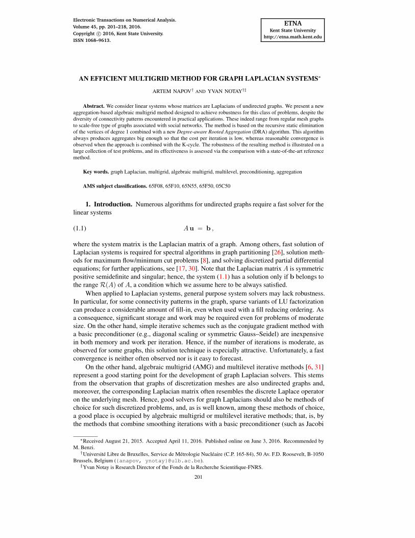
TABLE 1.1Total time (in seconds per million of nonzero entries in the matrix) needed to solve the graph Laplacian linear
system with various methods; n.c. means that the method has not converged in 1000 iterations; dagger symbol †
informs that the problem matrix comes from the University of Florida Sparse Matrix Collection [9]; double dagger‡ is for matrices from the LAMG test set suite [16]; the subscript lcc means that the graph has several connectedcomponents and the experiment was performed with the largest connected component.
Graph n nnz/n SGS AGMG Boomer LAMG Newdelaunay_n23† 8388608 7.0 n.c. 1.63 1.98 4.17 1.27
144† ‡ 144649 15.9 2.59 1.04 2.15 2.52 0.35soc-Slashdot0902‡lcc 25736 26.1 0.30 53.90 92.53 2.70 0.24
web-BerkStan‡lcc 282720 16.9 14.15 18.03 10.82 1.60 1.20
or Gauss–Seidel), and the approximate solution of a coarse representation of the probleminvolving fewer unknowns.
Yet, the performance of AMG methods with arbitrary graphs may be disappointing. Toillustrate this point, we provide in Table 1.1 the total solution time needed for some AMGapproaches to solve some graph Laplacian systems. The considered methods include standardAMG approaches: an aggregation-based method [19, 22] as implemented in the AGMGsoftware [23], and a classical Ruge–Stüben method [7, 27] as implemented in the BoomerAMG software [12] from the hypre package [13]; but also an AMG method by Livne andBrandt [17] which is specifically designed for graph Laplacians and implemented in theLAMG software [16]. For the sake of completeness, we also provide timings for symmetricGauss–Seidel preconditioning (SGS). The considered graphs represent a sample from thetest set used for the numerical experiments in Section 4.∗ In particular, the first two graphscorrespond to discretization meshes: two-dimensional (2D) mesh for delaunay_n23 andthree-dimensional (3D) one for 144, whereas soc-Slashdot0902 and web-BerkStanare social network graphs.
The results in Table 1.1 show that standard AMG approaches perform well for graphscorresponding to discretization meshes; regarding Ruge–Stüben AMG, this confirms the resultsin [3]. However, both AGMG and Boomer AMG encounter severe difficulties with socialnetwork graphs. On the other hand, LAMG is robust, but it is less efficient than PDE solvers onmesh graphs, and sometimes even not competitive with simple Gauss–Seidel preconditioning.
This raises the question: can we design a method that would be competitive with PDEsolvers on mesh graphs, and that would nevertheless be robust while never being significantlyslower than simple Gauss–Seidel preconditioning? The answer is given in the last column ofTable 1.1, where, anticipating on the following, we show the results obtained with the methodpresented in the next sections.
Eventually, it is worth noting that we do not present this new method as a kind of universalsolver, competitive with specialized methods for discrete scalar elliptic PDEs while able tohandle arbitrary graphs. Indeed, when designing the algorithms, we took benefit from the factthat, in most applications, graphs are either unweighted or have weights not varying muchin magnitude. We also assumed that all weights are positive, and hence the system matrixis always a symmetric M-matrix. As a result, the new method may be not appropriate for
∗See Section 4 for more details on the origin of the graphs and on the experiments setting; let us just mention herethat the conjugate gradient acceleration was used in all cases and that all software were used with default parameter,with the exception of Boomer AMG, considered with the same smoother as AGMG (that is, with a single forwardGauss–Seidel sweep as pre-smoother, and a single backward Gauss–Seidel sweep as post-smoother), and a coarsestgrid solver being 5 iterations of the symmetric Gauss–Seidel method with a coarsest grid of size at most 100 (insteadof 1 by default; this way we circumvent issues stemming from the singularity of the coarsest grid matrix, which boilsdown to the zero 1× 1 matrix when the coarsest grid contains a single unknown).
ETNAKent State University
http://etna.math.kent.edu
AN EFFICIENT MULTIGRID METHOD FOR GRAPH LAPLACIANS 203
PDE problems with anisotropy or jumping coefficients, and/or with a discretization that yieldspositive off-diagonal connections.
Regarding related works, we already mentioned the results from [3] and [17]. Morespecifically, in [3], the Ruge–Stüben AMG approach is theoretically analyzed and testedon mesh graphs. In [17], the Lean Algebraic Multigrid (LAMG) method is presented andshown to be quite robust, giving us motivation to take this method as state-of-the-art referencefor comparison. In particular, LAMG appears in [17] overall as efficient but more robustthan the Combinatorial Multigrid (CMG) method from [15]. This latter method is relatedto combinatorial subgraph preconditioners, introduced by Vaidya [32], and later analyzed in[4]. Several theoretically oriented works further develop the approach, near linear complexitybeing ultimately proved in [29]; however, as noted in [10], the estimates contain hiddenconstants that may be very large. In [10], an extensive numerical comparison is provided,which includes not just such subgraph preconditioners and CMG, but also PCG with ILU anddiagonal preconditioning, as well as some variants of aggregation-based AMG. The focusis on systems arising when applying interior point methods to minimum cost flow problems.The main conclusions are in line with our own findings summarized above: single levelpreconditioners can be effective but none of them is able to solve all the problems, whereasaggregation-based AMG variants perform well in general, but none of the tested aggregationalgorithms is robust in all cases.
The remainder of this paper is organized as follow. First, in the remainder of this introduc-tory section, we briefly recall the definitions of an undirected graph and its Laplacian matrix.Section 2 is an introduction to aggregation-based AMG methods, with a special emphasis onthe key components, namely the aggregation and the K-cycle. The new aggregation strategyis presented and motivated in Section 3, and the performance of the corresponding solver isfurther assessed on a large set of test graphs in Section 4. We end with some conclusions inSection 5.
Graph Laplacians. In this work we consider only undirected graphs. As a reminder,a graph G = (V,E) (also called simple graph) is given by a set V of vertices and a setE ⊂ V × V of edges. G is undirected if (i, j) ∈ E implies (j, i) ∈ E for every i, j ∈ V .An undirected graph is weighted if it has an associated positive weight function w : E 7→ R+
such that w(i, j) = w(j, i) for every (i, j) ∈ E . An unweighted graph is transformed into aweighted one by assigning the default weight 1 to all edges.
The Laplacian matrix of an undirected graph G (or its graph Laplacian) is the matrixA = (aij) such that, for all i 6= j ,
aij =
{−w(i, j) if (i, j) ∈ E ,
0 otherwise ,
whereas the diagonal entries are set up in such a way that A has zero row-sums:
aii = −∑j 6=i
aij .
Clearly, such a matrix A is symmetric and singular. Because it has nonpositive off-diagonalentries and nonnegative row-sums, it further turns out that it is a symmetric M-matrix, hencepositive semidefinite [2].
In what follows, we further assume that every vertex has at least one edge connectingit to another vertex; that is, there is no isolated vertices. This is not a restrictive assumption,since the unknowns in the graph Laplacian system corresponding to isolated vertices may haveany value, and the corresponding rows/columns can safely be deleted from the system. Inparticular, this assumption implies that aii > 0 for all i .
ETNAKent State University
http://etna.math.kent.edu
204 A. NAPOV AND Y. NOTAY
2. Aggregation-based multigrid methods.
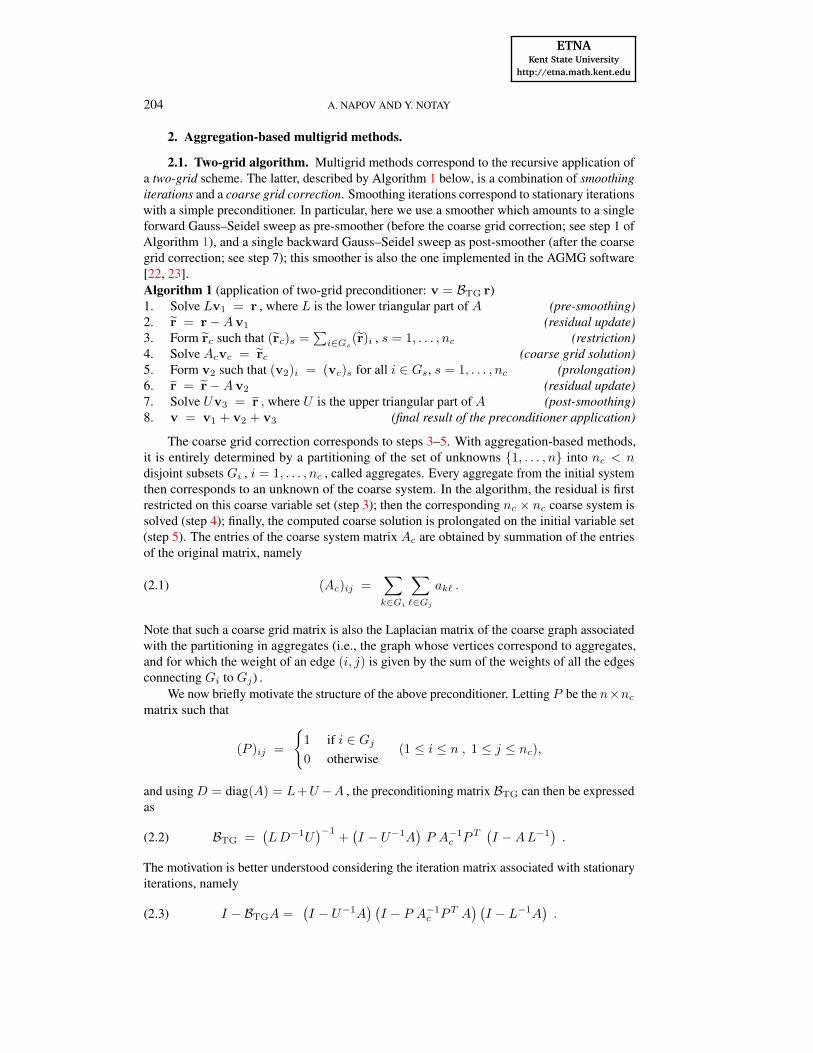
2.1. Two-grid algorithm. Multigrid methods correspond to the recursive application ofa two-grid scheme. The latter, described by Algorithm 1 below, is a combination of smoothingiterations and a coarse grid correction. Smoothing iterations correspond to stationary iterationswith a simple preconditioner. In particular, here we use a smoother which amounts to a singleforward Gauss–Seidel sweep as pre-smoother (before the coarse grid correction; see step 1 ofAlgorithm 1), and a single backward Gauss–Seidel sweep as post-smoother (after the coarsegrid correction; see step 7); this smoother is also the one implemented in the AGMG software[22, 23].Algorithm 1 (application of two-grid preconditioner: v = BTG r)1. Solve Lv1 = r , where L is the lower triangular part of A (pre-smoothing)2. r = r−Av1 (residual update)3. Form rc such that (rc)s =
∑i∈Gs
(r)i , s = 1, . . . , nc (restriction)4. Solve Acvc = rc (coarse grid solution)5. Form v2 such that (v2)i = (vc)s for all i ∈ Gs, s = 1, . . . , nc (prolongation)6. r = r−Av2 (residual update)7. Solve Uv3 = r , where U is the upper triangular part of A (post-smoothing)8. v = v1 + v2 + v3 (final result of the preconditioner application)
The coarse grid correction corresponds to steps 3–5. With aggregation-based methods,it is entirely determined by a partitioning of the set of unknowns {1, . . . , n} into nc < ndisjoint subsets Gi , i = 1, . . . , nc , called aggregates. Every aggregate from the initial systemthen corresponds to an unknown of the coarse system. In the algorithm, the residual is firstrestricted on this coarse variable set (step 3); then the corresponding nc × nc coarse system issolved (step 4); finally, the computed coarse solution is prolongated on the initial variable set(step 5). The entries of the coarse system matrix Ac are obtained by summation of the entriesof the original matrix, namely
(2.1) (Ac)ij =∑k∈Gi
∑`∈Gj
ak` .
Note that such a coarse grid matrix is also the Laplacian matrix of the coarse graph associatedwith the partitioning in aggregates (i.e., the graph whose vertices correspond to aggregates,and for which the weight of an edge (i, j) is given by the sum of the weights of all the edgesconnecting Gi to Gj) .
We now briefly motivate the structure of the above preconditioner. Letting P be the n×ncmatrix such that
(P )ij =
{1 if i ∈ Gj0 otherwise
(1 ≤ i ≤ n , 1 ≤ j ≤ nc),
and using D = diag(A) = L+U −A , the preconditioning matrix BTG can then be expressedas
(2.2) BTG =(LD−1U
)−1+(I − U−1A
)P A−1
c PT(I −AL−1
).
The motivation is better understood considering the iteration matrix associated with stationaryiterations, namely
(2.3) I − BTGA =(I − U−1A
) (I − P A−1
c PT A) (I − L−1A
).
ETNAKent State University
http://etna.math.kent.edu
AN EFFICIENT MULTIGRID METHOD FOR GRAPH LAPLACIANS 205
Thus, stationary iterations with BTG alternate coarse grid corrections (corresponding to theterm I − P A−1
c PT A , which is actually a projector) and smoothing iterations (correspondingto the terms I − L−1A and I − U−1A , which are the iteration matrices associated withforward and backward Gauss–Seidel, respectively). The efficiency of the approach relies onthe complementarity of these two sub-iterations: the coarse grid correction should be able tosignificantly reduce the error modes that are not efficiently damped by Gauss–Seidel iterations.
Nowadays algebraic multigrid methods are commonly used as preconditioners, especiallyif robustness is required. In particular, here the approach is combined with the conjugategradient method. This is possible because the resulting preconditioner is symmetric andpositive definite (SPD), as can be seen from (2.2) and the observations that L = UT while Dhas strictly positive diagonal entries. (In particular, the symmetry of the preconditioner is amajor motivation for choosing pre- and post-smoothing operators that are the transpose ofeach other.) Note that the systems to solve are singular, but compatible positive semidefinitesystems can be solved without problem by the conjugate gradient algorithm if one uses a SPDpreconditioner [14]; moreover the standard bound on the number of iterations applies, usingthe effective condition number κeff , defined as the ratio of the largest and the smallest nonzeroeigenvalue of the preconditioned matrix.
A slight difficulty comes from the coarse grid correction step. Indeed, with (2.1), onesees that, A having zero row-sum, Ac will have zero row-sum as well; i.e., will be singular.The issues involved by a singular coarse grid matrix are analyzed in detail in [24]. It turnsout that in most cases there is no practical difficulty: on one hand, the coarse systems to besolved when applying BTG are always compatible; on the other hand, which solution is pickedup does not influence the following of the iterations (only the null space component of thecomputed solution is affected). In particular, this is true when the system matrix is symmetricand positive semidefinite, as is always the case in this work. From a more theoretical viewpoint,note, however, that (2.2) and (2.3) contain then an abuse of notation: one should substitute forA−1c the generalized inverse that is effectively used to implement step 4 in Algorithm 1.
2.2. Multigrid cycles. The coarse grid system solved at step 4 in Algorithm 1 is typicallystill too large to make the use of a direct solver affordable. Multigrid methods resort torecursion then: the coarse system is solved only approximately, using few iterations with thesame two-grid preconditioning approach, but applied at the coarse level. This also means that afurther coarser level is then defined; the related system is again solved with the same approach,etc. The recursion is stopped when the system matrix is small enough to allow the use of adirect solver. The stopping criterion used here is the coarse grid system size being below n1/3 ,where n is the size of the original (fine grid) system matrix. This criterion guarantees that thefactorization cost is below the cost of one multiplication by A independently of the occurringfill-in.
The number and the nature of the iterations used for the solution of the coarse gridsystem is determined by the multigrid cycle. In particular, the V-cycle resorts to a singleiteration, the W-cycle uses two stationary iterations, and the K-cycle [25] uses two iterationsas well, but in combination with a Krylov acceleration. In the symmetric case, the Krylovaccelerator is the flexible conjugate gradient method [21] (more precisely FCG(1)); the flexiblevariant is required since the preconditioner used at any level but the bottom one is a variablepreconditioner.
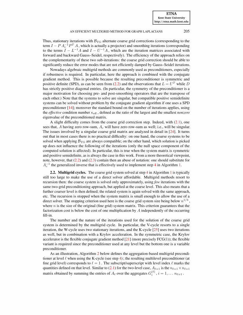
As an illustration, Algorithm 2 below defines the aggregation-based multigrid precondi-tioner at level ` when using the K-cycle (see step 4) ; the resulting multilevel preconditioner (atfine grid level) corresponds to ` = 1 . The subscript/superscript with level index ` marks thequantities defined on that level. Similar to (2.1) for the two-level case, A`+1 is the n`+1×n`+1
matrix obtained by summing the entries of A` over the aggregates G(`)i , i = 1, . . . n`+1 .
ETNAKent State University
http://etna.math.kent.edu
206 A. NAPOV AND Y. NOTAY
Algorithm 2 (application of K-cycle multigrid preconditioner at level `: v = B` r)1. Solve L`v1 = r , where L` is the lower triangular part of A` (pre-smoothing)2. r = r−A` v1 (residual update)3. Form rc such that (rc)s =
∑i∈G(`)
s(r)i , s = 1, . . . , n`+1 (restriction)
4. if n`+1 ≤ n1/3 (coarse grid solution)solve A`+1vc = rc with a sparse direct solver
elsecompute vc with 2 FCG(1) iterations for A`+1vc = rc with preconditioner B`+1
end if5. Form v2 such that (v2)i = (vc)s for all i ∈ G(`)
s , s = 1, . . . , n`+1 (prolongation)6. r = r−A` v2 (residual update)7. Solve U`v3 = r , where U` is the upper triangular part of A` (post-smoothing)8. v = v1 + v2 + v3 (final result of the preconditioner application)
Let us now briefly elaborate on the complexity of the aforementioned recursive algorithms.Denoting by nnz(A2) , . . . , nnz(AL) the number of nonzero entries in the successive coarsegrid matrices, the operator complexity
CA = 1 +
L∑`=2
nnz(A`)nnz(A)
is used to assess the memory requirements associated with the multigrid method; it is indepen-dent of the multigrid cycle being used. Roughly speaking, the amount of space needed to storethe preconditioner is CA times the amount of space needed to store the fine grid matrix A .With the V-cycle, CA also characterizes the computational cost needed for one application ofthe preconditioner. Roughly speaking, it can be assessed as CA times the cost of the smoothingiterations at fine grid level.
However, the W- and K-cycles are more costly, and their complexity is better characterizedby the weighted complexity
CW = 1 +
L∑`=2
2`−1 nnz(A`)nnz(A)
.
The factor 2`−1 takes into account the two iterations performed at each level, and hence thecost needed for one application of the preconditioner is roughly equal to CW times the cost ofsmoothing iterations at fine grid level (see [19] for details).
Both complexities are typically controlled by ensuring that the coarsening rationnz(A`−1)/nnz(A`) is above a given threshold at each level ` . For the operator complexityCA to be below, say, 3 , it is enough to request that the coarsening ratio remains above 3/2 forall levels. On the other hand, for the weighted complexity to stay below the same value 3 , thecoarsening ratio should be two times larger, namely at least 3 .
The extra cost of the W- and K-cycles comes together with less restrictive requirements onthe associated two-grid cycle. This is especially the case for the K-cycle, for which numericalexperiments consistently show good behavior even when the two-grid condition number is byfar larger than allowed by the theory available so far.
It is false to think that any combination of a two-grid method and a multigrid cycle leadsto a sensible multigrid method, especially if AMG methods are considered. Typically, when itis foreseen to use the V-cycle, the design is focused on the criteria needed to obtain a level-independent convergence rate; in “difficult” cases, this is often incompatible with coarseningratio values sufficiently large for allowing a sensible use of the K-cycle. On the other hand,
ETNAKent State University
http://etna.math.kent.edu
AN EFFICIENT MULTIGRID METHOD FOR GRAPH LAPLACIANS 207
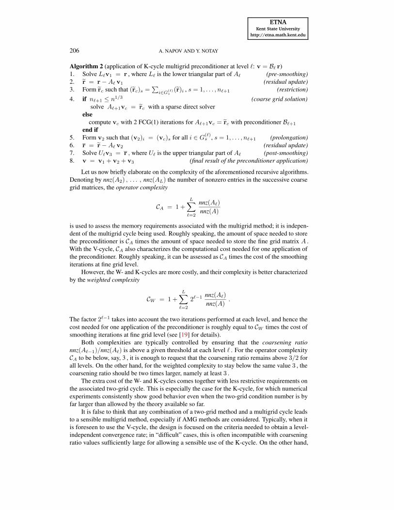
TABLE 3.1Condition number and coarsening ratio for a two-grid method based on several aggregation strategies. The
superscripts †, ‡ and the subscript lcc have the same meaning as in Table 1.1.
PA3κ=∞ DRAr=1 DRAr=2 DRAmix
Graph κeffnnz(A)nnz(A2) κeff
nnz(A)nnz(A2) κeff
nnz(A)nnz(A2) κeff
nnz(A)nnz(A2)
bcsstk29‡ 2.5 19.0 2.6 115.7 4.8 378.7 2.8 121.6144† ‡ 3.1 7.2 2.8 7.9 5.3 28.4 3.3 10.5t60k† ‡ 8.4 5.3 3.4 1.6 4.0 3.0 4.0 3.0
nopoly† 6.1 8.3 3.7 4.0 9.3 10.5 6.7 8.0as-22july06† 2.7 1.3 7.8 2.6 14.7 5.2 7.8 2.7
Oregon-2†lcc 2.5 1.4 6.1 3.8 11.3 10.7 6.1 3.9web-BerkStan‡lcc 24.1 3.2 85.5 34.8 481.8 69.6 85.5 39.9
when one has the K-cycle in mind, the primary objective is to keep CW reasonably small,whereas ensuring some minimal two-grid convergence properties is often enough. Then, againin “difficult” cases, using the V-cycle instead of the K-cycle may lead to a severe deteriorationof the convergence.
In the present work, we deliberately focus on the K-cycle, which seems to fit better withaggregation-based multigrid: on one hand, optimal V-cycle convergence is very difficult toobtain with mere aggregation, even for PDE problems [5, 31]; on the other hand, the controlof CW is easier than with other AMG approaches, since the number of nonzeros in the nextcoarse grid matrix can be decreased just by increasing the mean aggregates’ size. The AGMGmethod also illustrates that a cheap two-grid method in combination with the K-cycle canrepresent all in all a cost effective option [20, 22]. In this way, we also work in a directioncomplementary to that explored by Livne and Brandt [17], whose aggregation-based methodis primarily designed for the V-cycle, even if a fractional cycle (intermediate between V andW [6]) is finally used.
3. Coarse grid solution strategies for graph Laplacians.
3.1. Towards the new aggregation algorithm. We have seen in Table 1.1 that theAGMG solver is quite ineffective for certain types of graphs. In fact, this method correspondsto the framework described in the preceding section, and, looking into the details, it turns outthat the slowness comes from a weighted complexity CW that is unacceptably large.
Thus, we seek for a new aggregation algorithm capable to form larger aggregates whileensuring some minimal two-grid convergence properties. The results of our successive attemptsare illustrated in Table 3.1, where we consider a sample of test graphs that is representativeof the different types of difficulties met during our study. In this table, we focus on the basictwo-grid method and we report the two associated key quantities: on one hand, the effectivetwo-grid condition number κeff of the preconditioned matrix, and, on the other hand, thecoarsening ratio nnz(A)/nnz(A2) . As mentioned earlier, the values above 3 of this latterparameter are typically considered as acceptable.
The AGMG method [22, 19] uses a multiple pairwise aggregation strategy, which isnowadays popular in the context of PDE solvers. The strategy proceeds in several passes.During the first pass, pairs are formed via a pairwise matching procedure applied to the initialgraph. This gives aggregates of size at most 2, which is too low. Then, during the secondpass, the corresponding coarse matrix is temporarily formed and the process is repeated,forming pairs based on this matrix, and thus pairs of pairs with respect to the initial matrix (i.e.,
ETNAKent State University
http://etna.math.kent.edu
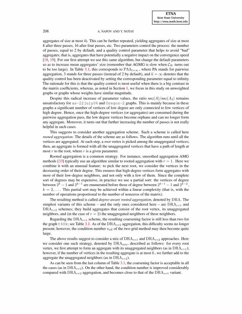
208 A. NAPOV AND Y. NOTAY
aggregates of size at most 4). This can be further repeated, yielding aggregates of size at most8 after three passes, 16 after four passes, etc. Two parameters control the process: the numberof passes, equal to 2 by default, and a quality control parameter that helps to avoid “bad”aggregates; that is, aggregates that have potentially a negative impact on the convergence speed[18, 19]. For our first attempt we use this same algorithm, but change the default parametersso as to increase mean aggregates’ size (remember that AGMG is slow when CW turns outto be too large). In Table 3.1, this corresponds to PA3κ=∞ , where PA stands for pairwiseaggregation, 3 stands for three passes (instead of 2 by default), and κ =∞ denotes that thequality control has been deactivated by setting the corresponding parameter equal to infinity.The rationale for this is that the quality control is most useful when there is a big contrast inthe matrix coefficients, whereas, as noted in Section 1, we focus in this study on unweightedgraphs or graphs whose weights have similar magnitude.
Despite this radical increase of parameter values, the ratio nnz(A)/nnz(A2) remainsunsatisfactory for as-22july06 and Oregon-2 graphs. This is mainly because in thesegraphs a significant number of vertices of low degree are only connected to few vertices ofhigh degree. Hence, once the high-degree vertices (or aggregates) are consumed during thepairwise aggregation pass, the low degree vertices become orphans and can no longer formany aggregate. Moreover, it turns out that further increasing the number of passes is not reallyhelpful in such cases.
This suggests to consider another aggregation scheme. Such a scheme is called hererooted aggregation. The details of the scheme are as follows. The algorithm runs until all thevertices are aggregated. At each step, a root vertex is picked among the unaggregated vertices;then, an aggregate is formed with all the unaggregated vertices that have a path of length atmost r to the root, where r is a given parameter.
Rooted aggregation is a common strategy. For instance, smoothed aggregation AMGmethods [33] typically use an algorithm similar to rooted aggregation with r = 1 . Here wecombine it with an unusual feature: to pick the next root, we consider the vertices in thedecreasing order of their degree. This ensures that high-degree vertices form aggregates withmost of their low-degree neighbors, and not only with a few of them. Since the completesort of degrees may be expensive, in practice we use a partial sort: the vertices of degreebetween 2k − 1 and 2k−1 are enumerated before those of degree between 2k−1 − 1 and 2k−2 ,k = 2, . . . . This partial sort may be achieved within a linear complexity (that is, with thenumber of operations proportional to the number of nonzeros of the matrix).
The resulting method is called degree-aware rooted aggregation, denoted by DRA. Thesimplest variants of this scheme – and the only ones considered here – are DRAr=1 andDRAr=2 schemes; they build aggregates that consist of the root vertex, its unaggregatedneighbors, and (in the case of r = 2) the unaggregated neighbors of these neighbors.
Regarding the DRAr=1 scheme, the resulting coarsening factor is still less than two forthe graph t60k; see Table 3.1. As of the DRAr=2 aggregation, this difficulty seems no longerpresent; however, the condition number κeff of the two-grid method may then become quitelarge.
The above results suggest to consider a mix of DRAr=1 and DRAr=2 approaches. Herewe consider one such strategy, denoted by DRAmix, described as follows: for every rootvertex, we first attempt to form an aggregate with its unaggregated neighbors (as in DRAr=1);however, if the number of vertices in the resulting aggregate is at most 6 , we further add to theaggregate the unaggregated neighbors (as in DRAr=2).
As can be seen from the last column of Table 3.1, the coarsening factor is acceptable in allthe cases (as in DRAr=2). On the other hand, the condition number is improved considerablycompared with DRAr=2 aggregation, and becomes close to that of the DRAr=1 variant.
ETNAKent State University
http://etna.math.kent.edu
AN EFFICIENT MULTIGRID METHOD FOR GRAPH LAPLACIANS 209
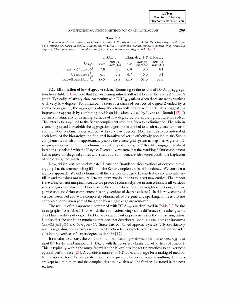
TABLE 3.2Condition number and coarsening ratios with respect to the original matrix A (and the Schur complement S) for
a two-grid method based on DRAmix alone, and on DRAmix combined with the recursive elimination of vertices ofdegree 1. The superscripts †, ‡ and the subscript lcc have the same meaning as in Table 1.1.
DRAmix Elim. deg. 1 & DRAmix
Graph κeffnnz(A)nnz(A2) κeff
nnz(S)nnz(A2)
nnz(A)nnz(A2)
as-22july06† 7.8 2.7 6.8 3.3 4.1Oregon-2†lcc 6.1 3.9 4.7 5.3 6.1
web-BerkStan‡lcc 85.5 39.9 85.5 51.5 52.3
3.2. Elimination of low-degree vertices. Returning to the results of DRAmix aggrega-tion from Table 3.1, we note that the coarsening ratio is still a bit low for the as-22july06graph. Typically, relatively slow coarsening with DRAmix arises when there are many verticeswith very low degree. For instance, if there is a chain of vertices of degree 2 ended by avertex of degree 1, the aggregates along the chain will have size 2 or 3. This suggests toimprove the approach by combining it with an idea already used by Livne and Brandt [17]. Itconsists in statically eliminating vertices of low degree before applying the iterative solver.The latter is thus applied to the Schur complement resulting from this elimination. The gain incoarsening speed is twofold: the aggregation algorithm is applied to an already smaller matrix,and the latter contains fewer vertices with very low degrees. Note that this is considered ateach level of the hierarchy: the fine grid iterative solver is effectively applied to the Schurcomplement; but, also, to approximately solve the coarse grid system at step 4 in Algorithm 2,we pre-process with the static elimination before performing the 2 flexible conjugate gradientiterations associated with the K-cycle. Eventually, we note that the resulting Schur complementhas negative off-diagonal entries and a zero row sum; hence, it also corresponds to a Laplacianof some weighted graph.
Now, which vertices to eliminate? Livne and Brandt consider vertices of degree up to 4,arguing that the corresponding fill-in in the Schur complement is still moderate. We consider asimpler approach. We only eliminate all the vertices of degree 1, which does not generate anyfill-in and thus does not require data structure manipulations to insert new entries. The impactis nevertheless not marginal because we proceed recursively: we in turn eliminate all verticeswhose degree is reduced to 1 because of the eliminations of all its neighbors but one, and wepursue until the Schur complement has only vertices of degree at least 2. In this way, chains ofvertices described above are completely eliminated. More generally speaking, all trees that areconnected to the main part of the graph by a single edge are removed.
The results of this approach combined with DRAmix are displayed in Table 3.2 for thethree graphs from Table 3.1 for which the elimination brings some difference (the other graphsdon’t have vertices of degree 1). One sees significant improvements in the coarsening ratios,but also that the condition number either does not deteriorate (web-BerkStan) or improves(as-22july06 and Oregon-2). Since this combined approach yields fully satisfactoryresults regarding complexity (see the next section for complete results), we did not considereliminating vertices of larger degree as done in [17].
It remains to discuss the condition number. Leaving web-BerkStan asides, κeff is atmost 6.7 for the combination of DRAmix with the recursive elimination of vertices of degree 1.This is typically within the range for which the K-cycle is known (in practice) to deliver nearoptimal performance [25]. A condition number of 6.7 looks a bit large for a multigrid method,but the approach can be competitive because the preconditioner is cheap: smoothing iterationsare kept to a minimum and the complexities are low; this will be further illustrated in the nextsection.
ETNAKent State University
http://etna.math.kent.edu
210 A. NAPOV AND Y. NOTAY
On the other hand, regarding web-BerkStan, κeff = 85.5 is certainly too large topretend that the method is free from any drawback. However, after looking closely at theresults for this specific graph, and also inspecting the results for complete test suite (see nextsection), we conclude that it is still far from a severe robustness failure. The main reasons forthis conclusion are as follows.
• The standard upper bound for the number of conjugate gradient iterations is equalto 68 for κeff = 85.5 and a 10−6 reduction in the residual norm. In practice,for a random right hand side (see next section), 53 iterations are needed with thetwo-grid preconditioner. This is large but still reasonable taking into account that,with nnz(A)/nnz(A2) > 50 , the weighted complexity is practically equal to 1; 53iterations with CW = 1 amount to about 18 iterations with CW = 3 .
• With such a large condition number, one could expect a significant deterioration in theconverge speed when switching from two-grid to multigrid solver, even if the latteris used with K-cycle. However, for this specific example, the number of iterationsgrows only from 53 to 68, which is still acceptable. We have no explanation for thisbehavior, besides the fact that, thanks to very large coarsening ratios, only 3 levelsare needed and, hence, the effects induced by the recursive use are minimal.
• We in fact deliberately include in Tables 3.1 and 3.2 the web-BerkStan graph forwhich conditioning issues are the most severe out of a collection of 142 examples.The iteration count of 68 corresponds to the maximum, and the number of iterationis actually larger than 35 in less than 4 % of the cases. Moreover, thanks to lowcomplexities, none of these cases corresponds to examples for which the solutiontime per nonzero is the largest: largest solution times are actually observed when thenumber of iteration is around 30 and the weighted complexity around 2.
3.3. Summary of the new method. We now briefly summarize the main features ofthe new preconditioner. When applied to system (1.1), it first recursively eliminates all thevertices of degree 1, yielding a reduced system with system matrix A1 . This system is solvedwith FCG(1), using the preconditioner defined by Algorithm 2 for ` = 1 , in which step 4 isslightly modified when n`+1 > n
1/31 , the vertices of degree 1 being first eliminated, and the 2
FCG(1) iterations being applied to the reduced Schur complement system. The aggregatesG
(`)i , i = 1, . . . , n`+1 , used at each level ` are obtained with the DRAmix scheme applied
to the Schur complement matrix resulting from the elimination of degree 1 vertices. Thecorresponding aggregation algorithm is explicitly given below for the sake of completeness.
Algorithm 3 DRAmix (Degree-aware Rooted Aggregation with mixed distance to root)1. Compute floor[log2(degree)] for all vertices2. nc ← 03. while there are vertices outside ∪nc
s=1Gs4. Select as root a vertex r not in ∪nc
s=1Gs with maximal value of floor[log2(degree(r))]5. nc ← nc + 1 and Gnc
= {r} ∪ {j /∈ ∪nc−1s=1 Gs | arj 6= 0}
6. if size(Gnc) ≤ 6Gnc ← Gnc ∪ {j /∈ ∪
nc−1s=1 Gs | ∃k ∈ Gnc : akj 6= 0}
end if7. end while
4. Numerical results. In this section we provide some further numerical evidence ofthe effectiveness of the new method. We begin by describing the extensive test set usedfor the experiments, providing details of the experimental setting, and commenting on therepresentation of the reported results. We then report on some key parameters that characterize
ETNAKent State University
http://etna.math.kent.edu
AN EFFICIENT MULTIGRID METHOD FOR GRAPH LAPLACIANS 211
the performance of the new method. Eventually, we report on the comparison of the newmethod with LAMG [16].
General setting. We considered all the graphs coming from the two following sources.• The University of Florida Sparse Matrix Collection [9], selecting the sparse matrices
whose description contains the keywords undirected and graph, as well as thematrices in the collection which are from (or also available in) Walshaw’s GraphPartitioning Archive [28]. In particular, most of the graphs from the 10th DIMACSchallenge [11] fall into this category.• The LAMG test set suite [16]†.
In both cases, only the graphs with more than 104 vertices have been considered. Moreover,according to the remark at the end of Section 1, we discarded the few graphs for which theratio between maximal and minimal weights exceeds 15. On the other hand, for graphs havingseveral connected components, only the largest one was considered for the tests.
This gives us a set of 142 graphs, of which 113 have more than 2 · 105 nonzero entries inthe corresponding graph Laplacian. This latter subset was used when elapsed time is reported.The remaining 29 graphs were excluded because absolute times were too small and subjectto large relative variations from run to run. Time experiments were performed by runninga Fortran 90 implementation of the method on a single core of a computing node with twoIntel XEON L5420 processors at 2.50 GHz and 16 Gb RAM memory. When considering theabsolute value of the reported times, it is good to remember that this machine dates back from2009.
Eventually, the right hand sides b in (1.1) were generated using a uniform randomdistribution with a fixed seed; the condition b ∈ R(A) was enforced by replacing the sogenerated b with its projection b− 1(bT1)/(1T1) , where 1 is the vector of all ones. In allcases, we used the flexible conjugate gradient method (FCG(1)) with the zero vector as initialapproximation, the stopping criterion being 10−6 reduction in the residual norm.
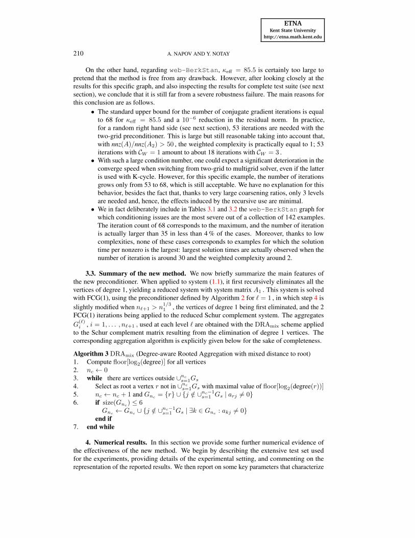
Numerical results are reported using bar diagrams, see Figure 4.2 for an example. Eachabscissa segment corresponds to an individual graph from the test set, and each bar based onthis segment is a reported value. The problems on the diagram are gathered in three groupsdefined below, depending on the value of the parameter p, which we define as the ratio betweenthe maximal and the average number of nonzeros per row. Note that p ≥ 1 in all cases; highvalues of p typically correspond to problems with strongly varying distribution of degrees. InFigure 4.1, we display the values of p as a function of the average number of nonzeros perrow (nnz/n , which is also the average degree plus 1). Somehow artificially, we distinct threeclasses based on the value of p (they are delimited by dashed horizontal lines on the figure).
• Group g1 corresponds to p < 1.2 , and mainly contains the regular mesh graphs.• Group g2 corresponds to 1.2 < p < 12 and includes some unstructured finite element
meshes, road network graphs, as well as some low-degree referencing graphs.• Group g3 corresponds to p > 12 , and contains social networks, e-mail, citation and
web referencing graphs. (This group should contain all scale-free type of graphs [1],but we were unable to determine whether all members of the group are scale free ornot.)
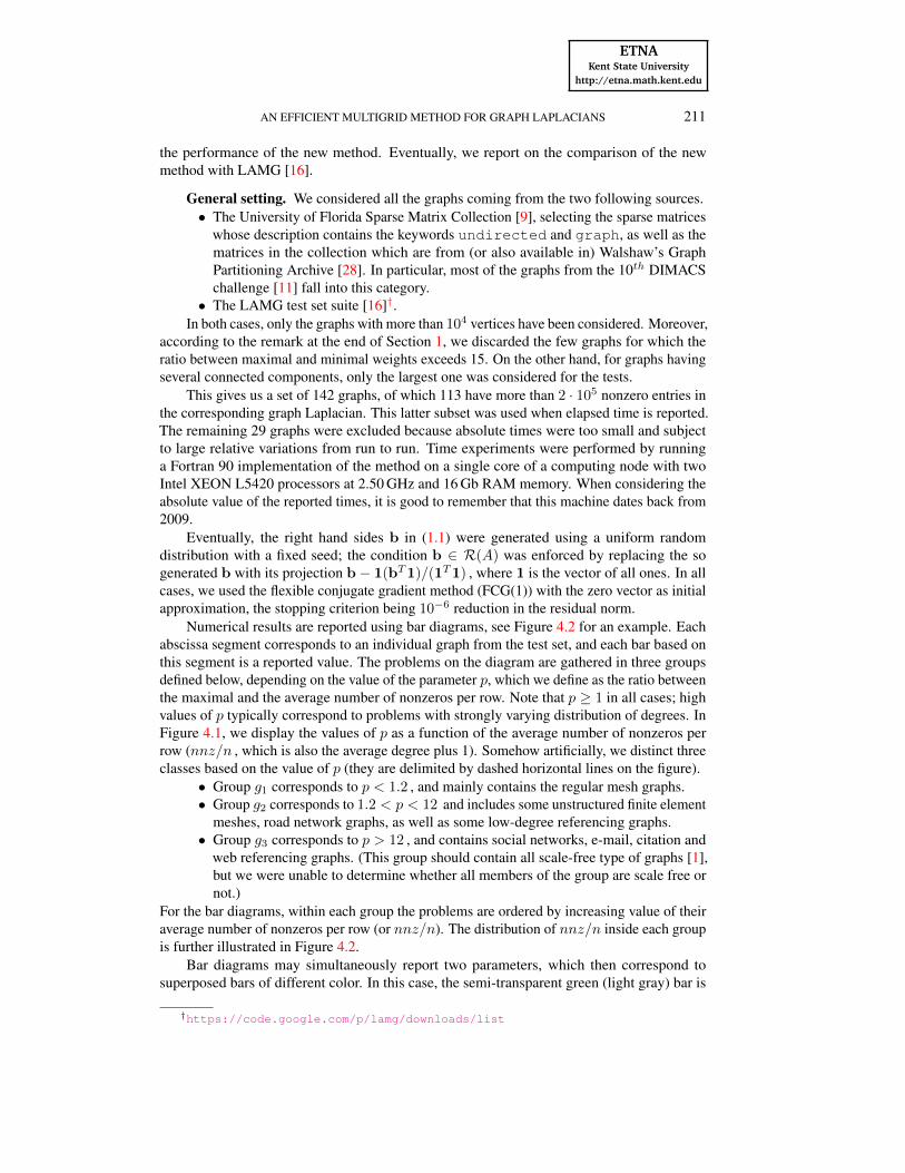
For the bar diagrams, within each group the problems are ordered by increasing value of theiraverage number of nonzeros per row (or nnz/n). The distribution of nnz/n inside each groupis further illustrated in Figure 4.2.
Bar diagrams may simultaneously report two parameters, which then correspond tosuperposed bars of different color. In this case, the semi-transparent green (light gray) bar is
†https://code.google.com/p/lamg/downloads/list

ETNAKent State University
http://etna.math.kent.edu
212 A. NAPOV AND Y. NOTAY
1
10
102
103
104
1 10 102 103
num
bero
fnon
zero
spe
rrow
:max
imal
/ave
rage
(p)
average number of nonzeros per row (nnz/n)
FIG. 4.1. The values of the parameter p and the average number of nonzeros per row (nnz/n) for the consideredproblems; the groups are separated by dashed lines.
1
10
100
g1 (by nnz/n) g2 (by nnz/n) g3 (by nnz/n)
nnz/n
FIG. 4.2. The distribution of the average number of nonzeros per row (nnz/n) within the groups g1, g2 andg3; the groups are separated by dashed lines; inside each group, the graphs are ordered by increasing number ofnonzero entries per row.
printed over the opaque blue (dark gray) bar; since the former bar is semi-transparent, the latterbar is still clearly visible, but the color of the overlapping area becomes dark green (gray).Hence, if the semi-transparent green bar is higher than the blue one, the diagram looks like theone on Figure 4.3. However, if the blue bar is higher, as is the case for most of the bars onFigure 4.8, the blue bar will remain partly uncovered.
Assessment of the new method. We start with the complexities of the new method (asdescribed in Section 2.2), reported on Figure 4.3. First note that the weighted complexityis below 2 for most of the problems, and always below 3. This means that the work neededfor one application of the multigrid preconditioning is in most cases below 2 times that ofsmoothing iterations at fine grid level. Since these latter amount to one forward and one
ETNAKent State University
http://etna.math.kent.edu
AN EFFICIENT MULTIGRID METHOD FOR GRAPH LAPLACIANS 213
0
1
2
3
g1 g2 g3
CWCA(bars overlap)
com
plex
ity
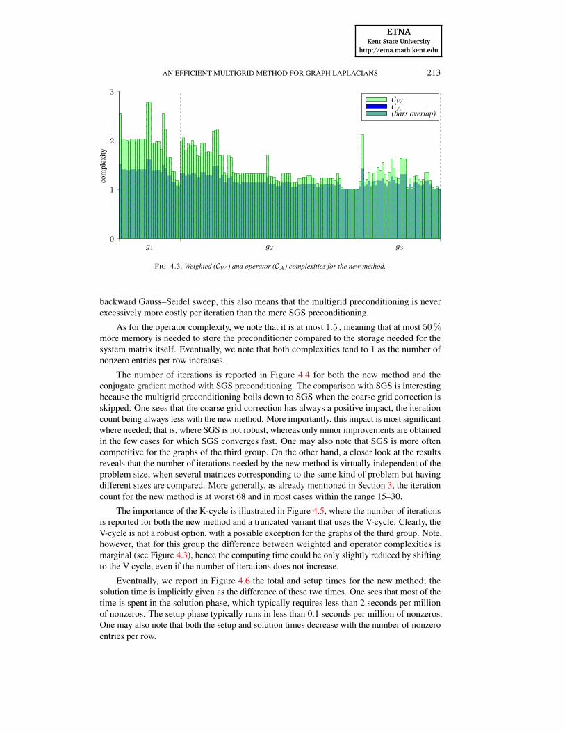
FIG. 4.3. Weighted (CW ) and operator (CA) complexities for the new method.
backward Gauss–Seidel sweep, this also means that the multigrid preconditioning is neverexcessively more costly per iteration than the mere SGS preconditioning.
As for the operator complexity, we note that it is at most 1.5 , meaning that at most 50 %more memory is needed to store the preconditioner compared to the storage needed for thesystem matrix itself. Eventually, we note that both complexities tend to 1 as the number ofnonzero entries per row increases.
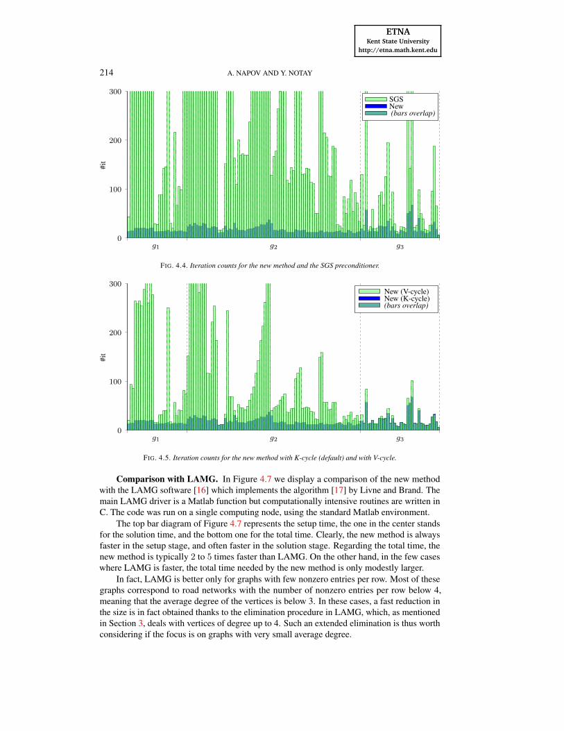
The number of iterations is reported in Figure 4.4 for both the new method and theconjugate gradient method with SGS preconditioning. The comparison with SGS is interestingbecause the multigrid preconditioning boils down to SGS when the coarse grid correction isskipped. One sees that the coarse grid correction has always a positive impact, the iterationcount being always less with the new method. More importantly, this impact is most significantwhere needed; that is, where SGS is not robust, whereas only minor improvements are obtainedin the few cases for which SGS converges fast. One may also note that SGS is more oftencompetitive for the graphs of the third group. On the other hand, a closer look at the resultsreveals that the number of iterations needed by the new method is virtually independent of theproblem size, when several matrices corresponding to the same kind of problem but havingdifferent sizes are compared. More generally, as already mentioned in Section 3, the iterationcount for the new method is at worst 68 and in most cases within the range 15–30.
The importance of the K-cycle is illustrated in Figure 4.5, where the number of iterationsis reported for both the new method and a truncated variant that uses the V-cycle. Clearly, theV-cycle is not a robust option, with a possible exception for the graphs of the third group. Note,however, that for this group the difference between weighted and operator complexities ismarginal (see Figure 4.3), hence the computing time could be only slightly reduced by shiftingto the V-cycle, even if the number of iterations does not increase.
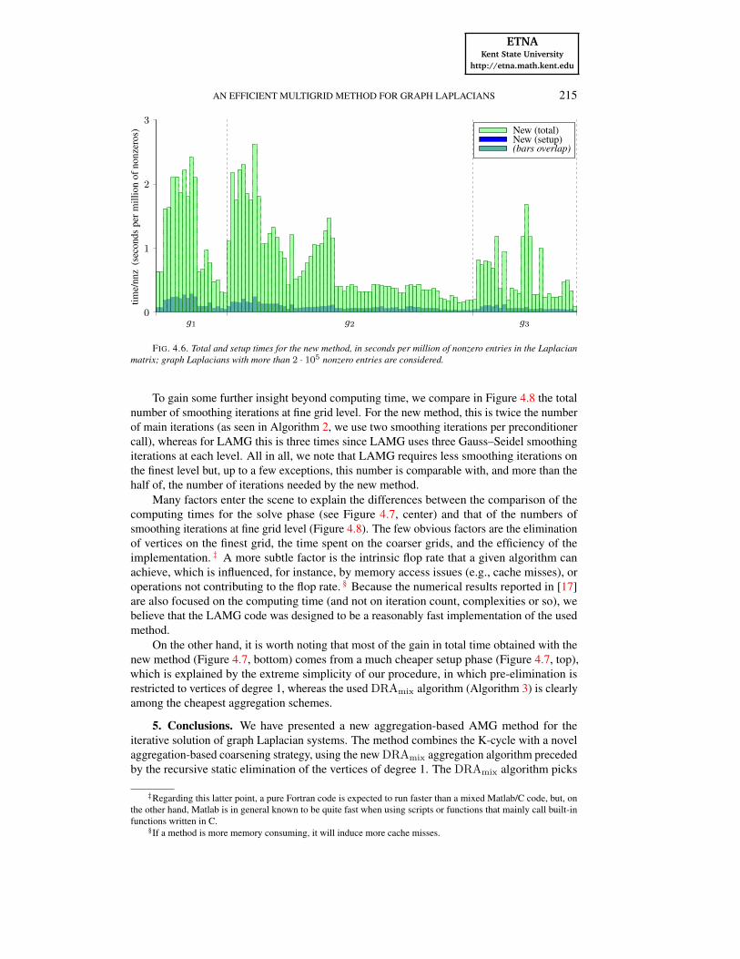
Eventually, we report in Figure 4.6 the total and setup times for the new method; thesolution time is implicitly given as the difference of these two times. One sees that most of thetime is spent in the solution phase, which typically requires less than 2 seconds per millionof nonzeros. The setup phase typically runs in less than 0.1 seconds per million of nonzeros.One may also note that both the setup and solution times decrease with the number of nonzeroentries per row.
ETNAKent State University
http://etna.math.kent.edu
214 A. NAPOV AND Y. NOTAY
0
100
200
300
g1 g2 g3
#it
SGSNew(bars overlap)
FIG. 4.4. Iteration counts for the new method and the SGS preconditioner.
0
100
200
300
g1 g2 g3
#it
New (V-cycle)New (K-cycle)(bars overlap)
FIG. 4.5. Iteration counts for the new method with K-cycle (default) and with V-cycle.
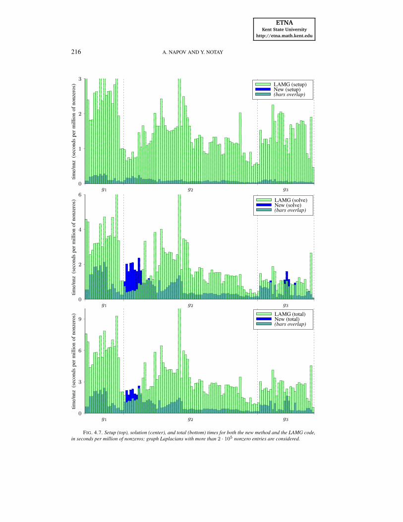
Comparison with LAMG. In Figure 4.7 we display a comparison of the new methodwith the LAMG software [16] which implements the algorithm [17] by Livne and Brand. Themain LAMG driver is a Matlab function but computationally intensive routines are written inC. The code was run on a single computing node, using the standard Matlab environment.
The top bar diagram of Figure 4.7 represents the setup time, the one in the center standsfor the solution time, and the bottom one for the total time. Clearly, the new method is alwaysfaster in the setup stage, and often faster in the solution stage. Regarding the total time, thenew method is typically 2 to 5 times faster than LAMG. On the other hand, in the few caseswhere LAMG is faster, the total time needed by the new method is only modestly larger.
In fact, LAMG is better only for graphs with few nonzero entries per row. Most of thesegraphs correspond to road networks with the number of nonzero entries per row below 4,meaning that the average degree of the vertices is below 3. In these cases, a fast reduction inthe size is in fact obtained thanks to the elimination procedure in LAMG, which, as mentionedin Section 3, deals with vertices of degree up to 4. Such an extended elimination is thus worthconsidering if the focus is on graphs with very small average degree.
ETNAKent State University
http://etna.math.kent.edu
AN EFFICIENT MULTIGRID METHOD FOR GRAPH LAPLACIANS 215
0
1
2
3
g1 g2 g3
time/
nnz
(sec
onds
perm
illio
nof
nonz
eros
) New (total)New (setup)(bars overlap)
FIG. 4.6. Total and setup times for the new method, in seconds per million of nonzero entries in the Laplacianmatrix; graph Laplacians with more than 2 · 105 nonzero entries are considered.
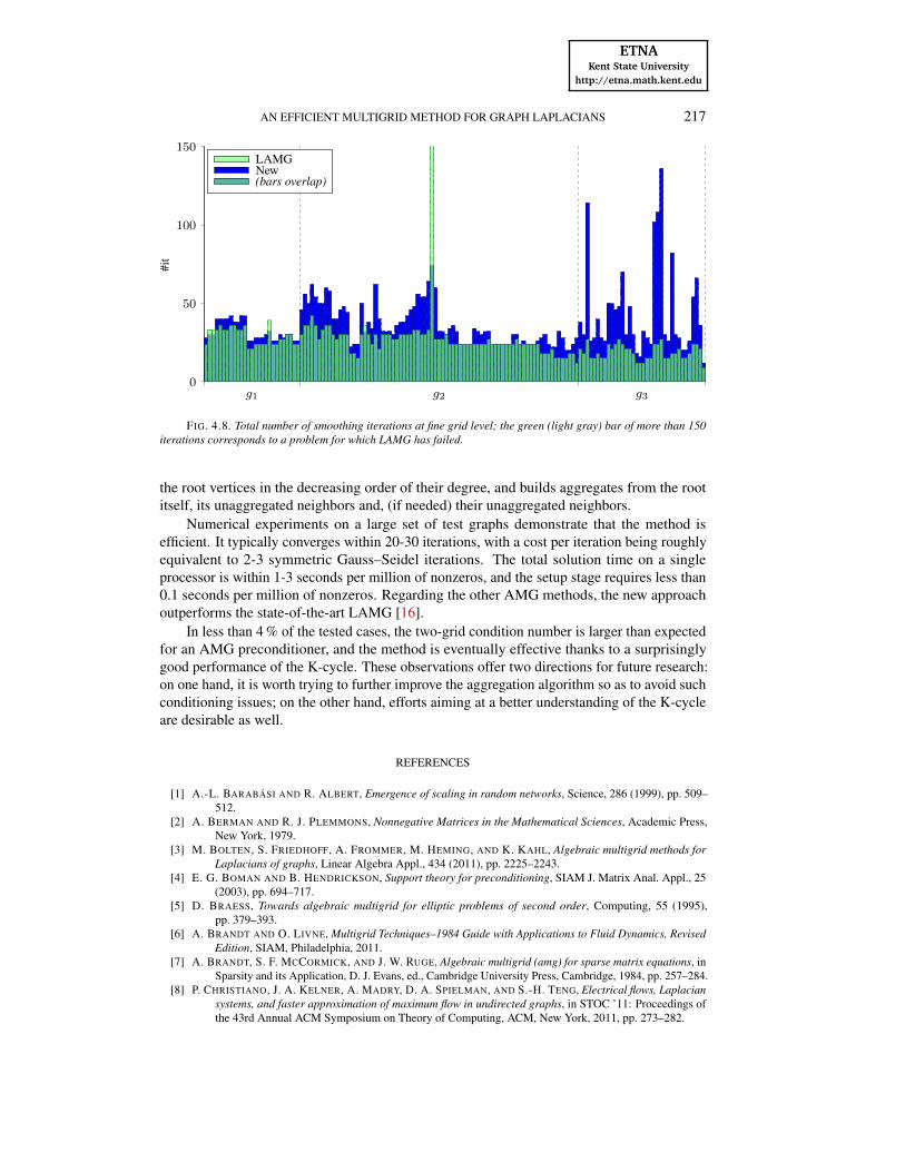
To gain some further insight beyond computing time, we compare in Figure 4.8 the totalnumber of smoothing iterations at fine grid level. For the new method, this is twice the numberof main iterations (as seen in Algorithm 2, we use two smoothing iterations per preconditionercall), whereas for LAMG this is three times since LAMG uses three Gauss–Seidel smoothingiterations at each level. All in all, we note that LAMG requires less smoothing iterations onthe finest level but, up to a few exceptions, this number is comparable with, and more than thehalf of, the number of iterations needed by the new method.
Many factors enter the scene to explain the differences between the comparison of thecomputing times for the solve phase (see Figure 4.7, center) and that of the numbers ofsmoothing iterations at fine grid level (Figure 4.8). The few obvious factors are the eliminationof vertices on the finest grid, the time spent on the coarser grids, and the efficiency of theimplementation. ‡ A more subtle factor is the intrinsic flop rate that a given algorithm canachieve, which is influenced, for instance, by memory access issues (e.g., cache misses), oroperations not contributing to the flop rate. § Because the numerical results reported in [17]are also focused on the computing time (and not on iteration count, complexities or so), webelieve that the LAMG code was designed to be a reasonably fast implementation of the usedmethod.
On the other hand, it is worth noting that most of the gain in total time obtained with thenew method (Figure 4.7, bottom) comes from a much cheaper setup phase (Figure 4.7, top),which is explained by the extreme simplicity of our procedure, in which pre-elimination isrestricted to vertices of degree 1, whereas the used DRAmix algorithm (Algorithm 3) is clearlyamong the cheapest aggregation schemes.
5. Conclusions. We have presented a new aggregation-based AMG method for theiterative solution of graph Laplacian systems. The method combines the K-cycle with a novelaggregation-based coarsening strategy, using the new DRAmix aggregation algorithm precededby the recursive static elimination of the vertices of degree 1. The DRAmix algorithm picks
‡Regarding this latter point, a pure Fortran code is expected to run faster than a mixed Matlab/C code, but, onthe other hand, Matlab is in general known to be quite fast when using scripts or functions that mainly call built-infunctions written in C.
§If a method is more memory consuming, it will induce more cache misses.
ETNAKent State University
http://etna.math.kent.edu
216 A. NAPOV AND Y. NOTAY
0
1
2
3
g1 g2 g3
time/
nnz
(sec
onds
perm
illio
nof
nonz
eros
) LAMG (setup)New (setup)(bars overlap)
0
2
4
6
g1 g2 g3
time/
nnz
(sec
onds
perm
illio
nof
nonz
eros
) LAMG (solve)New (solve)(bars overlap)
0
3
6
9
g1 g2 g3
time/
nnz
(sec
onds
perm
illio
nof
nonz
eros
) LAMG (total)New (total)(bars overlap)
FIG. 4.7. Setup (top), solution (center), and total (bottom) times for both the new method and the LAMG code,in seconds per million of nonzeros; graph Laplacians with more than 2 · 105 nonzero entries are considered.
ETNAKent State University
http://etna.math.kent.edu
AN EFFICIENT MULTIGRID METHOD FOR GRAPH LAPLACIANS 217
0
50
100
150
g1 g2 g3
#it
LAMGNew(bars overlap)
FIG. 4.8. Total number of smoothing iterations at fine grid level; the green (light gray) bar of more than 150iterations corresponds to a problem for which LAMG has failed.
the root vertices in the decreasing order of their degree, and builds aggregates from the rootitself, its unaggregated neighbors and, (if needed) their unaggregated neighbors.
Numerical experiments on a large set of test graphs demonstrate that the method isefficient. It typically converges within 20-30 iterations, with a cost per iteration being roughlyequivalent to 2-3 symmetric Gauss–Seidel iterations. The total solution time on a singleprocessor is within 1-3 seconds per million of nonzeros, and the setup stage requires less than0.1 seconds per million of nonzeros. Regarding the other AMG methods, the new approachoutperforms the state-of-the-art LAMG [16].
In less than 4 % of the tested cases, the two-grid condition number is larger than expectedfor an AMG preconditioner, and the method is eventually effective thanks to a surprisinglygood performance of the K-cycle. These observations offer two directions for future research:on one hand, it is worth trying to further improve the aggregation algorithm so as to avoid suchconditioning issues; on the other hand, efforts aiming at a better understanding of the K-cycleare desirable as well.
REFERENCES
[1] A.-L. BARABÁSI AND R. ALBERT, Emergence of scaling in random networks, Science, 286 (1999), pp. 509–512.
[2] A. BERMAN AND R. J. PLEMMONS, Nonnegative Matrices in the Mathematical Sciences, Academic Press,New York, 1979.
[3] M. BOLTEN, S. FRIEDHOFF, A. FROMMER, M. HEMING, AND K. KAHL, Algebraic multigrid methods forLaplacians of graphs, Linear Algebra Appl., 434 (2011), pp. 2225–2243.
[4] E. G. BOMAN AND B. HENDRICKSON, Support theory for preconditioning, SIAM J. Matrix Anal. Appl., 25(2003), pp. 694–717.
[5] D. BRAESS, Towards algebraic multigrid for elliptic problems of second order, Computing, 55 (1995),pp. 379–393.
[6] A. BRANDT AND O. LIVNE, Multigrid Techniques–1984 Guide with Applications to Fluid Dynamics, RevisedEdition, SIAM, Philadelphia, 2011.
[7] A. BRANDT, S. F. MCCORMICK, AND J. W. RUGE, Algebraic multigrid (amg) for sparse matrix equations, inSparsity and its Application, D. J. Evans, ed., Cambridge University Press, Cambridge, 1984, pp. 257–284.
[8] P. CHRISTIANO, J. A. KELNER, A. MADRY, D. A. SPIELMAN, AND S.-H. TENG, Electrical flows, Laplaciansystems, and faster approximation of maximum flow in undirected graphs, in STOC ’11: Proceedings ofthe 43rd Annual ACM Symposium on Theory of Computing, ACM, New York, 2011, pp. 273–282.
ETNAKent State University
http://etna.math.kent.edu
218 A. NAPOV AND Y. NOTAY
[9] T. A. DAVIS AND Y. HU, The University of Florida Sparse Matrix Collection, ACM Trans. Math. Software,38 (2011), pp. 87–94. Available athttp://www.cise.ufl.edu/research/sparse/matrices/.
[10] P. DELL’ACQUA, A. FRANGIONI, AND S. SERRA-CAPIZZANO, Accelerated multigrid for graph Laplacianoperators, Appl. Math. Comput., 270 (2015), pp. 193–215.
[11] 10th DIMACS Implementation Challenge – Graph Partitioning and Graph Clustering. Available athttp://www.cc.gatech.edu/dimacs10/downloads.shtml
[12] V. E. HENSON AND U. M. YANG, BoomerAMG: A parallel algebraic multigrid solver and preconditioner,Appl. Num. Math., 41 (2002), pp. 155–177.
[13] hypre 2.7.0 software and documentation. Available athttps://computation.llnl.gov/casc/linear_solvers/sls_hypre.html.
[14] E. F. KAASSCHIETER, Preconditioned conjugate gradients for solving singular systems, J. Comput. Appl.Math., 24 (1988), pp. 265–275.
[15] I. KOUTIS, G. L. MILLER, AND D. TOLLIVER, Combinatorial preconditioners and multilevel solvers forproblems in computer vision and image processing, Comput. Vision Image Understanding, 115 (2011),pp. 1638–1646.
[16] O. E. LIVNE, Lean Algebraic Multigrid (LAMG) Matlab Software, 2012. Release 2.1.1. Available athttp://lamg.googlecode.com.
[17] O. E. LIVNE AND A. BRANDT, Lean algebraic multigrid (LAMG): fast graph Laplacian linear solver, SIAMJ. Sci. Comput., 34 (2012), pp. B449–B522.
[18] A. NAPOV AND Y. NOTAY, Algebraic analysis of aggregation-based multigrid, Numer. Linear Algebra Appl.,18 (2011), pp. 539–564.
[19] , An algebraic multigrid method with guaranteed convergence rate, SIAM J. Sci. Comput., 43 (2012),pp. A1079–A1109.
[20] , Algebraic multigrid for moderate order finite elements, SIAM J. Sci. Comput., 36 (2014), pp. A1678–A1707.
[21] Y. NOTAY, Flexible conjugate gradients, SIAM J. Sci. Comput., 22 (2000), pp. 1444–1460.[22] , An aggregation-based algebraic multigrid method, Electron. Trans. Numer. Anal, 37 (2010), pp. 123–
146. Available at http://etna.mcs.kent.edu/vol.37.2010/pp123-146.dir[23] Y. NOTAY, AGMG Software and Documentation, 2011. Available at
http://homepages.ulb.ac.be/~ynotay/AGMG.[24] Y. NOTAY, Algebraic two-level convergence theory for singular systems, Tech. Report GANMN 15–01,
Université Libre de Bruxelles, Brussels, Belgium, 2015.[25] Y. NOTAY AND P. S. VASSILEVSKI, Recursive Krylov-based multigrid cycles, Numer. Linear Algebra Appl.,
15 (2008), pp. 473–487.[26] A. POTHEN, H. D. SIMON, AND K.-P. LIOU, Partitioning sparse matrices with eigenvectors of graphs, SIAM
J. Matrix Anal. Appl., 11 (1990), pp. 430–452.[27] J. W. RUGE AND K. STÜBEN, Algebraic multigrid (AMG), in Multigrid Methods, S. F. McCormick, ed., vol. 3
of Frontiers in Applied Mathematics, SIAM, Philadelphia, 1987, pp. 73–130.[28] A. J. SOPER, C. WALSHAW, AND M. CROSS, A combined evolutionary search and multilevel optimisation
approach to graph partitioning, J. Global Optim., 29 (2004), pp. 225–241.[29] D. SPIELMAN AND S.-H. TENG, Nearly-linear time algorithms for graph partitioning, graph sparsification,
and solving linear systems, in Proceedings of the 36th Annual ACM Symposium on Theory of Computing,L. Babai, ed., ACM, New York, 2004, pp. 81–90.
[30] D. A. SPIELMAN, Algorithms, graph theory, and linear equations in Laplacian matrices, in Proceedings ofthe International Congress of Mathematicians, vol. IV, R. Bhatia, A. Pal, G. Rangarajan, V. Srinivas, andM. Vanninathan, eds., World Scientific, Singarpore, 2010, pp. 2698–2722.
[31] K. STÜBEN, An introduction to algebraic multigrid, in Multigrid, U. Trottenberg, C. W. Oosterlee, andA. Schüller, eds., Academic Press, London, 2001, pp. 413–532 (Appendix A).
[32] P. M. VAIDYA, Solving linear equations with symmetric diagonally dominant matrices by constructing goodpreconditioners. Unpublished manuscript.
[33] P. VANEK, J. MANDEL, AND M. BREZINA, Algebraic multigrid based on smoothed aggregation for secondand fourth order problems, Computing, 56 (1996), pp. 179–196.