An Evaluation of Edge Line Striping as a Traffic Calming Technique … · 2008-05-24 · Edge Line Striping as a Traffic Calming Technique Eric J. Lamb, PE January 13, ... The researcher

An Evaluation of

Edge Line Striping

as a

Traffic Calming Technique

Eric J. Lamb, PE

January 13, 2002

1

I. Introduction

Background

Traffic calming is a significant topic of discussion in many cities throughout the

United States. While traffic calming devices have been widely deployed in other parts of

the world, the use of such technology has gained in popularity within the last decade.

Traffic calming devices come in many shapes and forms. Roundabouts, traffic circles,

chicanes and diverters all seek to impact speeds by deflecting the direct line of travel in

a horizontal manner, while treatments like speed humps and raised crosswalks create

physical barriers for vehicles. Ewing (1) states in Traffic Calming: State of the Practice

that “the purpose of traffic calming is to reduce the speed and volume of traffic to

acceptable levels” in order to improve livability, reduce accidents, and create a safer

environment for bicyclists and pedestrians.

Certain types of traffic calming devices seek to reduce vehicle speeds by

narrowing the amount of pavement available for vehicular travel. These devices include

chokers, center island narrowings, and bulbouts, which are also known as neck downs

or intersection narrowings. Previous studies have demonstrated a 4% reduction in

vehicle speeds using roadway narrowings (1).

Many communities have considered the application of lane stripes that delineate

the right edge of the travel lane on streets that provide more than 24 feet of pavement.

The premise behind this application is drivers will perceive there is less pavement

available for travel and may reduce their speeds in response. Such edge lines are

frequently employed to delineate the edge of pavement on rural highways, but are rarely

used in urban areas due to the prevalence of curb and gutter roadway cross-sections

(2).

2

The installation of horizontal or vertical deflection devices for traffic calming can

be costly. In 2001, the City of Raleigh conducted a study analyzing the impacts of speed

humps, installing 13 temporary rubber speed humps of and 16 asphalt speed humps at a

cost of $80,000 (3). Roundabouts can require additional right-of-way acquisition at

intersections. Substantial curb line modifications are required to install neckdowns and

medians. By comparison, lane striping applications are relatively cheap, and most

municipalities and state agencies have the existing resources to apply edge lines with

ease. Pavement marking options also do not create conflicts with emergency vehicle

response, which has been a major complaint of traditional traffic calming devices.

As communities continue to consider the use of edge lines as a traffic calming

device, the actual impact on vehicle speeds must be evaluated.

Purpose and Scope

The purpose of this research was to evaluate the impacts of applying outside

edge-line stripes on wide suburban streets. This research focuses specifically on

establishing 12-foot travel lanes via the application of a 4” white stripe on streets

between 38 and 40 feet in width from face-to-face of curbs.

This project began in August 2001 in conjunction with the City of Raleigh

Department of Transportation. The Raleigh City Council authorized participation in this

research study on September 4, 2001, and provided funding for the application of the

stripes and allocated City resources for data collection. The edge lines were applied at

the four sites on November 11, 2001, and data collection concluded in December 2001.

The product of this study is a before-and-after evaluation of the effectiveness of edge

lines as traffic calming devices in Raleigh, North Carolina.

The researcher used spot speed studies to test the effectiveness of this

treatment. Statistical tests were conducted to evaluate the significance of changes in

3

speeds relative to changes observed at a control site. The researcher made

recommendations to traffic engineers regarding the applicability of this treatment as a

traffic calming measure, and provided recommendations for future study of this

treatment.

Report Outline

A literature review of current practices of edge line treatments is included in

Chapter II. The site selection process and criteria established by the researcher is

provided in Chapter III. This chapter also contains detailed descriptions of the

characteristics of each site included in the study.

A description of the methodology employed in this study is explained in

Chapter IV. Methods of data collection and statistical analysis are also provided in this

section. Chapter V presents the analysis of the study data for each site and compares

the results to control site data. A summary and recommendations of this research is

provided in Chapter VI.

4

II. Literature Review

The purpose of the literature review is to provide background for the research

and establish current practices regarding use of the proposed treatment.

Previous Research

Two studies were found that directly address the use of pavement marking to

reduce driver speeds. In her paper on human factors and roadway design, Smiley (5)

references a 1997 Transport Canada study authored by the IBI Group on non-

enforcement methods of speed control. Smiley discusses a direct correlation between

driver speeds and lane and shoulder widths, but states that the IBI Group study

reviewed multiple techniques for traffic calming and found that changes in roadway

appearance (i.e., pavement markings) do not influence driver speeds. The researcher

attempted to locate documentation of this research but was unable to do so prior to the

conclusion of this study. Smiley asserts that drivers reduce speeds based solely upon

risk perception, such as sharp curves and steep shoulders, and side friction, i.e., heavy

pedestrian usage and on-street parking.

Lum (6) conducted a pavement marking study of narrow lane widths in Orlando,

Florida in 1984. This study used single and double white edge lines to create 9-foot

lanes with shoulders of varying width in each direction on two facilities in the Orlando

area. These facilities utilized a broken double-yellow centerline with 10-foot stripes

spaced 30 feet apart. Lum indicates the edge line treatment applied in his study had

little or no effect on vehicle speeds.

Several problems with this study were apparent to the researcher. The study

sites were not randomly selected but were chosen based upon citizen complaints of

excessive speeding. Parking allowances differed between the two sites studied, and

5

one of the study sites only allowed 925 feet of treatment to be evaluated. Lum

conducted “after” counts only two weeks after the installation and did not appear to

employ any statistical analyses to the collected data.

Current Usage

The researcher found several instances of usage or recommended usage of

edge line striping or similar treatments as a traffic calming method.

Ewing (1) cites a project conducted in Portland, Oregon where bike lanes were

installed concert with speed humps. The North Ida Avenue Project indicated a 2-5 mph

reduction in 85th percentile speeds when bike lanes were applied after speed humps

were installed. Ewing does not cite any instances of study where edge lines or bike

lanes were independently applied as traffic calming devices.

The City of Lynchburg, Virginia, attempted to use lane striping as a traffic calming

measure on Sheffield Drive due to excessive speeding (7). The installation of edge lines

occurred circa 1986 and created 11-foot travel lanes with 7-foot parking lanes in each

direction. No before and after data was available from the report, however the

documentation did provide speed data from 1986 and from prior to the study. This data

indicated that while speeding remains a problem on Sheffield Drive, operating speeds in

2000 were several miles per hour lower than speeds measured in 1986.

However, several instances in the literature suggest edge lines or bike lanes are

suitable traffic calming treatments. FHWA’s Traffic Calming website (8) offers bike lanes

as an example of a traffic calming treatment. Howard County, Maryland cites edge lines

as a potential speed reduction device in their Community Speed Control Program (9). A

draft study prepared by Remington and Vernick Engineers (10) for Wilmington, Delaware

recommended edge line treatments to reduce speeds in the Old Newark area. However,

6

the study suggests the treatment may be more effective when used in concert with other

types of traffic calming devices.

Conclusion

The actual effects of edge line striping on adjacent vehicle speeds are not clear

from the current literature. Recommended usage by several communities seems to

contradict previous research related to the matter. A statistically controlled field

evaluation of edge line treatments is needed to document the effects on driver behavior.

7

III. Site Characteristics

This section describes the site selection criteria used to select candidate sites for

this study. This section explains the details of the selection process and provides a brief

description of each site selected for the application of the edge line treatment.

Selection Criteria

To qualify for selection in this study, sites had to satisfy multiple criteria in order

to provide uniform conditions. These factors included street classification, street width,

roadway section, existing pavement marking, and bike route designation.

The City of Raleigh classifies streets hierarchically via the City’s Streets,

Sidewalks, and Driveway Access Handbook (4), which dictates a prescribed roadway

cross section for each class of facility. The City’s standard for collector streets is a two-

Figure III-1: Typical City of Raleigh Collector Street

8

lane 40-foot wide face-to-face curb and gutter section whose purpose is to channel

traffic from residential and commercial areas to thoroughfare system roadways. These

collector streets may serve as boundaries for developments with limited points of

access, or they may have a neighborhood character with single or multifamily residential

development directly fronting the street. Collector streets in Raleigh are typically posted

for 35 mph and are constructed to a 40-mph design speed per AASHTO standards.

Some collector streets have double-yellow centerlines installed as prescribed by

MUTCD thresholds (2), which creates an 18-foot travel lane from centerline to the edge

of pavement. While this section allows through traffic to operate comfortably adjacent to

on-street parking or bicycle users, collector streets are the subject of frequent speeding

complaints according to City of Raleigh Department of Transportation (RDOT)

personnel.

The study proposed to install edge lines in a manner that created 12-foot travel

lanes on collector streets with preexisting double-yellow centerlines. Installing edge

lines in this manner along collector streets with 40-foot face-to-face curb and gutter

sections would provide two 12-foot travel lanes and 8 feet of shoulder space from the

edge line to the face of the curb. The researcher determined this space would be

sufficient for continued use as on-street parking or bicycle traffic, if the space was used

as such prior to the study.

Research projects generally utilize a minimum longitudinal exposure of 0.3 miles

in order to ensure adequate exposure to the treatment. The researcher established a

minimum application length of approximately 2,000 feet in order to satisfy this exposure

need.

Since the installation of this treatment would visually resemble a bike lane and

could lead to the encouragement of use as such, the researcher restricted the scope of

the study to roadways currently classified and signed as bike routes within the City of

9

Raleigh’s bike route system. No additional bicycle signage or lane marking was

proposed as part of this study. Segments of sufficient length were identified by

correlating the City of Raleigh’s Bike Route Map with Wake County GIS roadway data.

This methodology identified 26 potential sites for field evaluation of existing conditions.

The researcher visited each site in order to determine the width and cross-

section of the roadway, to establish the existence of a double-yellow centerline, and to

guarantee the uniformity of the pavement marking within the desired study area. Sites

with three-lane striping or designated left turn lanes within the site limits were discarded

due to the horizontal deflection that would be created by edge line application relative to

these existing pavement markings. Sites with posted speeds above or below 35 mph

were not considered for this study.

Two of the proposed sites exceeded the 40-foot face-to-face curb and gutter

section and were discarded. The researcher determined that an edge line application on

streets exceeding the study width criteria would create a shoulder space in excess of

8 feet, which could potentially be confused for an additional travel lane and could create

an unsafe situation. One site was discarded due to the asymmetrical application of the

double-yellow centerline.

Several of the sites were discarded due to insufficient width, however two of the

sites identified for field evaluation maintained a 38-foot face-to-face curb and gutter

section. This width was consistent with an older collector road design standard utilized

by the City. The application of an edge line 12 feet from the double-yellow centerline on

this section would produce a clear shoulder space of 7 feet from the edge line to the face

of the curb. The researcher determined that this width was sufficient to maintain on-

street parking and to allow bicycle travel, and the study criteria was modified to include

38-foot face-to-face curb and gutter roadways.

10

Ten sites were identified as viable candidates for uniform application of the edge

line treatment. Of these candidate sites, four were selected at random to receive the

application of the edge line striping; the need for randomization is discussed in Chapter

IV. One site was also randomly selected from the candidate site pool to serve as a

control site. The Raleigh City Council’s approval of this study mandated coordination

and notification of property owners within the application areas and requested that sites

be removed from consideration if opposed by the residents. In response to this

requirement, two additional sites were randomly selected from the candidate site pool to

serve as alternate application sites, if necessary. All property owners within the limits of

the application sites were notified by mail of the project, and information concerning the

study was reported by local newspaper and television media. The researcher received

no responses from impacted property owners concerning this study, and the four

application sites initially selected for the study were retained for the duration of the

project.

Site Descriptions

This section briefly describes the characteristics of the four application sites and

the control site selected for the study.

Site 1 – Brookside Drive, Watauga Street to Glascock Street – 2400 feet

Brookside Drive is a north-south roadway in central Raleigh that has a 38-foot

face-to-face curb and gutter section with sidewalks on both sides. Adjacent land uses

include single family residential with direct driveway connections, with multifamily

residential and vacant commercial property interspersed. There is a city park and a

large cemetery along the east side of the street adjacent to the application area. Two

residential side streets intersect the roadway within the project limits. On-street parking

11

and pedestrians were observed in the field. This portion of Brookside Drive also supports

a City bus route.

The roadway grade is mostly flat with minor horizontal curvature, however there

is a significant horizontal curve with a moderate vertical grade increase at southern end

of project. The northern end of the project terminates at a signalized intersection with

Glascock Street, while the southern terminus at Watauga Street is controlled by a four-

way stop condition.

Site 2 – Rainwater Road, North Ridge Drive to Hunting Ridge Drive – 2000 feet

Rainwater Road is a north-south route located in north Raleigh and provides a

40-foot face-to-face curb and gutter section with sidewalk on one side. Adjacent

development is almost exclusively single-family residential with direct driveway

connections. There is an area golf course that abuts the roadway midway along the

project limits; there is an unmarked golf cart crossing at this location. On-street parking

and pedestrians were observed in the field. One residential side street intersects the

roadway within the project limits.

The roadway grade is flat at each end of the project with minor horizontal

curvature. There is a low area in the vicinity of the golf course with moderate vertical

curvature on each approach. The northern terminus of the project is controlled by a two-

way stop condition at Hunting Ridge Road. North Ridge Drive is controlled by a stop

condition at Rainwater Drive.

Site 3 – Sawmill Road, Bluffridge Drive to Lead Mine Road – 3600 feet

Sawmill Road is an east-west route located in north Raleigh and provides a 40-

foot face-to-face curb and gutter section with sidewalk on one side. Adjacent

development varies throughout the project limits. From Bluffridge Drive to Harbor Drive,

12

development is exclusively single-family residential with no direct driveway connections.

Private community recreational facilities exist on both sides of the road between Harbor

Drive and Valley Run Drive. Each facility has a single direct driveway connection to

Sawmill Road. From Valley Run Drive to east of Breckon Way, there is multifamily

attached housing along the north side with no direct driveway connections and single-

family residential along the south side with direct driveway access. East of Breckon

Way, there is a shopping center with driveway access along the north side and a church

with driveway access along the south side. West of the primary shopping center

driveway, the striping pattern changes to provide a left turn into the shopping center. No

on-street parking or pedestrians were observed in the field. Four residential side streets

intersect the roadway within the project limits.

Horizontal and vertical curvatures vary greatly throughout the project limits.

From The Pointe to Harbor Drive, there is a steady downgrade coupled with a sustained

horizontal curve. The roadway is flat between Harbor Drive and Valley Run Drive in

another sustained horizontal curve. East of Valley Run Drive, there is a steady incline

which levels off near Breckon Way. The western terminus is controlled by a traffic signal

at Lead Mine Road. Bluff Ridge is stop sign controlled at its intersection with Sawmill

Road.

Site 4 – St. Albans Drive, Hardimont Road to Benson Drive – 2800 feet

St. Albans Drive is an east-west route located in north Raleigh and provides a

40-foot face-to-face curb and gutter section with sidewalk on one side. Land within the

project limits is mostly undeveloped. There is a large office building with both direct and

indirect driveway accesses located on the north side west of Benson Drive. East of

Hardimont Road, there are several single family residences along the north side, none of

which have direct driveway access to St. Albans Drive. No on-street parking or

13

pedestrians were observed in the field. There are no side streets intersecting the

roadway within the project limits.

From Hardimont Road to a roadway creek culvert, the roadway is mostly flat with

a slight downgrade in the vicinity of the creek crossing. The remainder of the project is a

sustained incline with moderate horizontal curvature. Both Hardimont Road and Benson

Drive are stop sign controlled at St. Albans Drive at the project termini.

Control Site – Lineberry Drive, Trailwood Drive to Trailwood Hills Drive – 2900 feet

Lineberry Drive is an east-west route located in southwest Raleigh and provides

a 40-foot face-to-face curb and gutter section with sidewalk on one side. Development

within the project limits is a mix of single and multifamily residential with no direct

driveway access. No on-street parking or pedestrians were observed in the field. There

are four residential side streets intersecting the roadway within the project limits. From

Trailwood Drive to Trailwood Hills Drive, there is a steady downgrade with mild

horizontal curves. The western end of the project terminates at a stop sign condition at

Trailwood Drive. At the eastern terminus, Trailwood Hills Drive is stop sign controlled at

its intersection with Lineberry Drive.

Summary

The project sites selected for evaluation in this study were based on criteria that

were consistently applied, providing uniform sites for an unbiased evaluation of the

proposed treatment.

14

IV. Evaluation Methodology

This chapter explains the methodology utilized in this study in order to evaluate

the effectiveness of the edge line treatment.

Experiment Design

This study was conducted as a before-and-after experiment examining the

potential speed reduction of edge line applications. Before-and-after studies are easily

understood by both technical staff and non-technical citizens, but if not conducted

properly can produce misleading results. The Manual of Traffic Engineering Studies

identifies seven distinct drawbacks to conducting before-and-after studies:

• The length of time required between the decision to conduct an experiment

and the achievement of a conclusion;

• The difficulty in designing an experiment while treatments are being

implemented or have already been implemented;

• The novelty effect of the treatment, causing drivers to react unusually or not

react immediately;

• Instability – reactions to the treatment which are unstable or random;

• History – changes in the measure of effectiveness due to external factors

(i.e., changes in posted speed, enforcement);

• Maturation – changes in the measure of effectiveness due to trends or larger

patterns; and,

• Regression to the mean – the tendency of fluctuating characteristics to return

to typical values after a period of time (11).

The researcher chose to conduct a simple before-and-after experiment with a

control site for this evaluation. The researcher anticipated the length of time required to

15

conduct the study and planned the sequence of approvals, installation, and data

collection accordingly. Since each analysis site would consist of evaluation after

installation of a new treatment, no post-hoc analysis would be conducted. A 30-day

“warm-up” period between deployment of the treatment and collection of after data was

used to overcome the novelty effect.

In order to overcome any instability, the study proposed to conduct data

collection at each location in both the before and after periods for a duration of 24 hours.

The researcher verified the adequacy of the sample size at each location via statistical

analysis in order to ensure proper sample sizes were obtained for 90%, 95% and 99%

confidence intervals.

By using a 30-day warm up period between installation of the treatment and

collection of after data, the researcher maintained a short study duration, thereby

overcoming problems related to history and maturation. The researcher also contacted

the Raleigh Police Department to ensure no special speed enforcement programs

occurred during the study period at any of the project sites.

Several measures reduced the effects of regression to the mean. The

researcher randomly selected each site for the application of edge lines from a pool of

candidate sites. The researcher also inspected the results of the study to ensure a

Poisson distribution of the experimental data. The use of a control site also further

reduced any potential problems caused by regression to the mean, as well as any

influence of either history or maturation.

Data Collection Methodology

The general purpose of traffic calming is to reduce the speed or volume of traffic

to levels that better accommodate non-motorized vehicle uses within and adjacent to the

roadway. The researcher selected spot speed as the measure of effectiveness for this

16

study to determine if the application of edge line created a reduction in vehicle speeds

within the project sites.

The researcher used GIS mapping to identify potential points for field data

collection within the middle third of each project site. The location of each data point

was field adjusted by the researcher to minimize the influence of four factors, ranked by

order of importance:

1) inadequate sight distance;

2) extreme or sudden changes in vertical grade;

3) extreme or sudden changes in horizontal alignment; and,

4) proximity of any adjacent intersections or traffic generators.

Upon determining the final location of the count station, the researcher painted

markings on the asphalt to maintain the location through both the before and after

phases of the study. Traffic counts in each direction were taken at the same location.

The researcher utilized automated data collection devices to obtain spot speeds

for this study. RDOT maintains multiple PEEK automated pneumatic tube counters to

collect volume and speed data periodically throughout the city. When used for speed

studies, the units utilize a pair of tubes spaced at a fixed width to measure the differential

between axle hits for each vehicle across each tube, thereby calculating a spot speed for

a given vehicle. Each pair of tubes is stretched across the road to the double-yellow

centerline and is unavoidable by drivers within the lane of traffic being surveyed.

Before counts were conducted by RDOT on weekdays between October 31,

2001 and November 6, 2001; weather conditions were clear and dry during each data

collection period. The counters collected 24 hours of field data, which was processed by

RDOT staff and summary information from each station was given to the researcher.

17

Installation

The Raleigh City Council and RDOT administration agreed to cover the costs

associated with the edge line installation by utilizing an open pavement marking contract

with Roadmark Corporation. The City Council stipulated that the application of the paint

for the edge lines should be made in a temporary manner so as to wear away within a

shorter period of time than normal pavement markings. The researcher discussed this

requirement with Roadmark personnel and with RDOT staff, who both agreed that a light

paint application could maintain a normal appearance for the duration of the study and

meet the semipermanency requirement stipulated by the City Council.

Figure IV-1: Brookside Drive after Edge Line Application

Roadmark agreed to maintain the contract’s unit cost for paint application, $0.07

per linear foot, provided the roadway premarking was handled by the researcher. The

researcher conducted premarking of the pavement with RDOT personnel, measuring the

location of the paint application exactly 12 feet from the center of the double-yellow

18

centerline to guarantee a uniform lane width throughout each project site. Breaks in the

striping were provided at each intersection with a side street. The edge lines were

treated with standard fiberglass beads for reflectivity and were applied at a rate

consistent with normal application on city streets. The total cost of the application was

$1308.23 for 18,689 linear feet of edge lines for all four application sites.

Given their appearance and their designation as bike routes, the researcher

acknowledged the potential for increased bicycle use of these striped roadways. The

researcher directed the application of the stripes in a manner consistent with bike lane

striping. The edge line application was truncated 100 feet short of stop conditions at

Sites 1 and 2 in order to reduce conflicts for turning cyclists.

Statistical Analyses

The researcher employed the use of several statistical tools to determine

whether any variation in speeds was the result of the treatment and if any such changes

were statistically significant. The Manual of Transportation Engineering Studies

recommends establishing a minimum sample size for statistical analysis of a given

statistic of interest for spot speed studies (11). Minimum sample size is established with

the following formula:

2

222

2)2(

EUKSN +

= , where

N = Minimum Sample Size

S = Estimated Standard Deviation of Sample

K = Constant for Desired Confidence Level

U = Constant for Desired Percentile Speed

E = Permitted Error in Average Speed Estimate

The Manual recommends estimating S = 5.0 mph and provides constants of

K = 2.58 for 99% confidence level and U = 1.04 for analysis of 85th percentile speeds.

19

The researcher chose a permitted error of + 1.0 mph, calculating the minimum required

sample size of 769 counts in each direction.

The researcher used the t-test to determine statistical significance of the before

and after data, as recommended in the Manual of Transportation Engineering Studies

(11). Since the researcher was only interested in the speed reduction potential of the

treatment, the researcher used a one-tailed t-test for this analysis.

To compare the application site data to the control site data, the researcher

employed the use of an odds ratio, which is a comparison of the proportion of each

sample. An odds ratio value of 1.0 represents a neutral value, signifying no difference in

the compared proportions, while numbers approaching zero or infinity represent large

differences in the comparison. This analysis requires normalized data free of any

regression influence.

The odds ratio is a matrix analysis, as follows:

Treatment Control

Before A B

After C D

where the odds ratio = AD/BC. Standard deviation for the odds ratio is computed

by the following formula:

DCBAS 1111

+++= .

The t-statistic for this analysis is calculated as the natural log of the odds ratio

divided by the standard deviation of the odds ratio, which is then compared to critical

t-statistic at the desired level of confidence. A calculated t-statistic less than the critical

t-statistic indicates no effect of the treatment and acceptance of the null hypothesis.

20

The researcher compared the proportions of drivers exceeding the speed limit for

before and after periods at each site versus the control site. This data was normalized

to the proportion of speed limit violations per 1000 observations at each site.

Summary

The methodology utilized by the researcher was sound and reliable, accounting

for known threats to the reliability of the analysis. The field evaluation of the edge line

treatment was conducted within the anticipated timeframe of the researcher. Data from

two counts were disregarded due to anomalies in the speed data; this data was not

Poisson distributed, rendering statistical analysis unreliable for this study. These data

anomalies may be attributable to mechanical error or to human error in the field

placement of the traffic counters.

The remainder of the data collected in this study satisfied the Poisson distribution

and sample size requirements established for this study. The analysis methodology

outlined here is applied to this data in the next chapter.

21

V. Analysis of Results

The researcher collected before and after data at four edge line application sites

and one control site by the methods outlined in the previous chapter. This field data is

provided for review in Appendix B of this report. Graphical comparisons of the frequency

data for each site are included in Appendix C.

The researcher tested three hypotheses for this study, using the t-statistic as the

basis for acceptance or rejection of these hypotheses at the 90%, 95% and 99% levels

of confidence. The null hypotheses tested were:

• The mean speed in the after period was greater than or equal to the mean

speed in the before period;

• The 50th percentile speed in the after period was greater than or equal to the

50th percentile speed in the before period; and

• The 85th percentile speed in the after period was greater than or equal to the

85th percentile speed in the before period.

Site 1 – Brookside Drive

Data was collected at this site on October 31, 2001 and on December 19, 2001

for a period of 24 hours during each count. The field equipment recorded 1,753 counts

in both directions in the before period and 1,951 counts in both directions in the after

period. A summary of the before and after field data is provided in table V-1. Before

and after comparisons of the mean vehicle speed, the 50th percentile speed, the 85th

percentile speed, and the standard deviation are provided for each site in each direction.

Graphical comparisons of relative and cumulative frequency data for this site are

included in Figures C-1 through C-4.

22

Table V-1: Comparison of Descriptive Speed Statistics at Site 1

The researcher tested results of the field data against the three hypotheses using

the t-test. Table V-2 displays the results of this hypothesis testing. The null hypotheses

were accepted at all levels of confidence in each direction, therefore the treatment had

no significant effect on reducing vehicle speeds at this location.

Table V-2: Results of Hypothesis Testing at Site 1

Accept or Reject Hull Hypothesis at Significance: Null

Hypothesis Difference from Before to After

Calculated t-statistic 90% 95% 99%

Northbound Mean Speed +0.18 -0.516 Accept Accept Accept 50th Percentile -0.16 0.458 Accept Accept Accept 85th Percentile -0.01 0.029 Accept Accept Accept

Southbound Mean Speed +0.96 -3.086 Accept Accept Accept 50th Percentile +0.67 -2.154 Accept Accept Accept 85th Percentile +0.96 -3.086 Accept Accept Accept

Site 2 – Rainwater Road

Data was collected at this site on November 6, 2001 and on December 18, 2001






NB NB SB SBBefore After change Before After change

Avg Speed 34.74 34.92 0.18 35.17 36.13 0.9650%ile 35.78 35.62 -0.16 35.87 36.54 0.6785%ile 41.56 41.55 -0.01 41.22 42.18 0.96

S 7.65 6.93 -0.72 6.92 6.82 -0.10

23




Data for the southbound before period did not meet the minimum sample size

established by the study. This data also contained anomalies within the distribution of

speeds within two categories. 490 counts were recorded in the 1-19 mph category, and

36 counts were recorded in the 55-60 mph category, representing 82.9% and 6.1% of

the population, respectively. This data is not Poisson distributed, therefore southbound

data for this location was discarded from the study. The researcher discussed possible

sources for this discrepancy with RDOT staff, who suggested the automated data

collection device for this count may have been improperly installed in the field or may not

have been properly calibrated.

The researcher tested results of the northbound field data against the three

hypotheses using the t-test. Table V-4 displays the results of this hypothesis testing.

The null hypotheses were accepted at all levels of confidence for the northbound

direction, therefore the treatment had no significant effect on reducing vehicle speeds at

this location.

NB NB SB SBBefore After change Before After change

Avg Speed 34.16 35.20 1.04 15.75 34.56 18.8150%ile 33.92 35.76 1.84 11.86 35.40 23.5485%ile 39.48 41.00 1.52 27.81 39.81 12.00

S 5.88 6.11 0.23 13.30 6.30 -6.99

24





Northbound Mean Speed +1.04 -5.562 Accept Accept Accept 50th Percentile +1.84 -9.840 Accept Accept Accept 85th Percentile +1.52 -8.129 Accept Accept Accept

Site 3 – Sawmill Road












were accepted at all levels of confidence in the eastbound direction, therefore the

treatment had no significant effect on reducing eastbound vehicle speeds at this

location.

EB EB WB WBBefore After change Before After change

Avg Speed 40.71 40.77 0.06 40.47 39.97 -0.5050%ile 41.04 41.15 0.11 39.87 39.54 -0.3385%ile 45.19 45.20 0.01 44.90 44.37 -0.53

S 4.28 4.26 -0.02 4.24 3.95 -0.29

25





Eastbound Mean Speed +0.06 -0.783 Accept Accept Accept 50th Percentile +0.11 -1.436 Accept Accept Accept 85th Percentile +0.01 -0.131 Accept Accept Accept

Westbound Mean Speed -0.50 6.329 Reject Reject Reject 50th Percentile -0.33 4.177 Reject Reject Reject 85th Percentile -0.53 6.709 Reject Reject Reject

Data for the westbound direction demonstrated a reduction in speeds in the three

categories of analysis, and the null hypothesis was rejected at all levels of confidence for

this direction. Although the null hypothesis was rejected, the practical reduction in

vehicle speeds was very slight and did not represent a substantive change in vehicle

speeds from the before period. Further analysis of the westbound data is addressed in

the comparison with the control site later in this chapter.

Site 4 – St. Albans Drive

Data was collected at this site on October 31, 2001, November 1, 2001 and on

December 18, 2001 for a period of 24 hours during each count. The field equipment

recorded 4,621 counts in both directions in the before period and 3,526 counts in both

directions in the after period. A summary of the before and after field data is provided in

table V-7. Before and after comparisons of the mean vehicle speed, the 50th percentile

speed, the 85th percentile speed, and the standard deviation are provided for each site in

each direction. Graphical comparisons of relative and cumulative frequency data for this

site are included in Figures C-13 through C-16.

26




were accepted at all levels of confidence in each direction, therefore the treatment had

no significant effect on reducing vehicle speeds at this location.





Eastbound Mean Speed +0.43 -2.017 Accept Accept Accept 50th Percentile +0.29 -1.360 Accept Accept Accept 85th Percentile +0.12 -0.563 Accept Accept Accept

Westbound Mean Speed +1.12 -4.914 Accept Accept Accept 50th Percentile +0.80 -3.510 Accept Accept Accept 85th Percentile +0.79 -3.466 Accept Accept Accept

Control Site – Lineberry Road


for a period of 24 hours during each count. The field equipment recorded 5261 counts in

both directions in the before period and 5,229 counts in both directions in the after

period. A summary of the field data for the before and after study periods is provided in

table V-9. Comparisons of the mean vehicle speed, the 50th percentile speed, the 85th



Avg Speed 38.91 39.34 0.43 37.69 38.81 1.1250%ile 39.21 39.50 0.29 38.26 39.06 0.8085%ile 45.86 45.98 0.12 44.87 45.66 0.79

S 7.44 7.03 -0.41 6.72 6.79 0.08

27

Graphical comparisons of relative and cumulative frequencies for this site are included in

Figures C-17 through C-20.

Table V-9: Comparison of Descriptive Speed Statistics at Control Site

Data recorded for eastbound traffic on Lineberry Drive included a discrepancy in

the category of vehicles travelling over 50 mph. 107 vehicles were recorded in this

range, representing four percent of the total observations for this site. This data is not

Poisson distributed, therefore data for the eastbound direction of travel was disregarded

for comparison in this study. Sources for the discrepancy of the data may be similar to

those described for Site 2. Westbound data did not experience the same type of

variation and appears to be Poisson distributed. This data was used as the source of

comparison for the other field data evaluated in this study.

Odds Ratio Analysis

The odds ratio methodology described in Chapter IV for comparing the

application sites with the control site was applied. The majority of the comparisons were

within one standard deviation of the neutral value, signifying that the proportion of drivers

exceeding the speed limit at the application sites before and after the edge line

installation were consistent with the proportions observed at the control. The null

hypothesis for the odds ratio test is as follows:

• Odds ratio null hypothesis: The change in proportion of drivers exceeding the

speed limit before and after the edge line application at the test sites was less


Avg Speed 38.85 36.38 -2.47 37.96 37.61 -0.3550%ile 38.72 36.63 -2.09 38.68 38.35 -0.3385%ile 44.35 41.91 -2.44 42.82 42.60 -0.22

S 6.63 5.81 -0.81 5.71 5.47 -0.24

28

than the change in proportion of drivers exceeding the speed limit at the

control site.

The odds ratio for northbound data at Site 2 exceeded one standard deviation,

however since the site registered an increase in traffic exceeding the speed limit after

the edge line installation, the null hypothesis is accepted for this location. Southbound

data was not included in this analysis due to discrepancies in this data as described

previously in this chapter. The t-statistic calculated for each site was less than the

critical t-value at 90%, 95% and 99% levels of confidence, therefore the null hypothesis

is accepted for all study sites. The results of the odds ratio analysis are shown in Table

V-10.

Table V-10: Results of Odds Ratio Analysis

Accept or Reject Null Hypothesis at Significance: Site Odds Ratio Standard

Deviation Calculated t-statistic 90% 95% 99%

Site 1 NB 1.028 0.078 0.349 Accept Accept Accept Site 1 SB 0.993 0.077 -0.094 Accept Accept Accept Site 2 NB 0.847 0.080 -2.075 Accept Accept Accept Site 2 SB No analysis No analysis No analysis N/A N/A N/A Site 3 EB 0.998 0.069 -0.023 Accept Accept Accept Site 3 WB 0.993 0.069 -0.106 Accept Accept Accept Site 4 EB 0.952 0.072 -0.678 Accept Accept Accept Site 4 WB 0.993 0.074 -0.098 Accept Accept Accept

Despite the statistically significant reduction in observed westbound speeds at

Site 3, comparison to the control site indicates this reduction cannot be validated against

the data from the control site.

29

VI. Summary and Conclusions

The purpose of traffic calming devices is to reduce the speed of traffic in

communities in order to improve livability, reduce accidents, and create a safer

environment for bicyclists and pedestrians. In order for a traffic calming device to be

effective, the treatment must reduce vehicle speeds below the normal level of operation

for a similar untreated facility. These treatments can force drivers to react physically by

altering the horizontal pathway of the vehicle, or they can also impede vehicle progress

by vertical deflection. Treatments that change driver perception of available roadway

width, such as neckdowns, have also been shown to reduce vehicle speeds.

Edge lines have been installed in other communities in the US and have been

touted as a potential traffic calming measure. The current literature does not provide

any documentation of previous evaluations to verify this assertion. Therefore, the

purpose of this research was to evaluate the potential speed reduction of edge line

striping on wide two-lane suburban streets.

The researcher identified ten potential sites for study in Raleigh, North Carolina.

These sites were identified based on multiple criteria including street width, existing

pavement marking, and preexisting classification as a bike route. The researcher

randomly selected four application sites and a control site from the candidate pool in

order to conduct a before and after study. Spot speeds were used as the measure of

effectiveness for this study. Data collection occurred during October 2001 and

November 2001 before the edge lines were installed. This treatment took place in

November 2001 and a 30-day warm-up period was observed. The after data were

collected in December 2001. Data for one direction at one application site and for one

direction at the control site was discarded due to significant anomalies in the distribution

of the data and insufficient sample size.

30

Findings

The researcher analyzed each site individually by direction of travel in the before

and after period. Statistical tests were conducted to evaluate the significance of

changes between the two periods at the application sites relative to changes observed at

the control site. Only one of the seven analyses demonstrated a statistically significant

reduction in vehicle speeds, but comparison to the control site negated the validity of this

decrease. The remainder of the site analyses showed no statistically significant or

practical reduction in vehicle speeds. Therefore, the application of edge line stripes as

conducted in this study does not appear to have any impact in reducing vehicle speeds

and should not be considered as a useful traffic calming application.

Recommendations for Similar Studies

The rejection of data from the control site and from the application site may have

been avoided if the data had been scrutinized prior to the application of the treatment.

The researcher had not conducted analysis of spot speed studies prior to this study and

was not aware that the data represented a significant deviation from normal patterns. In

the event the researcher had noticed these anomalies in the data, additional data

collection could have been conducted at the problem locations prior to the installation of

the treatment.

This evaluation was conducted in mostly suburban areas with a variety of land

uses and access patterns. Similar studies may wish to evaluate whether this treatment

could be applicable or effective in more urbanized areas. In addition, data collection

concerning bicycle usage within the project sites before and after the application was not

conducted as part of this study and should be considered for future evaluations.

31

Recommendations for Future Research

The results of this study establish an effective baseline for future research

regarding edge line striping. Future studies should consider evaluations of similar

treatments establishing lane widths less than 12 feet as was evaluated in this study.

Evaluation of this treatment in conjunction with additional bicycle signage or bike lane

pavement marking may also be worth evaluating.

Recommended use in the current literature suggests combining this treatment

with other types of traffic calming devices. If sufficient data can be obtained and if all the

relevant variables can be controlled accordingly, this may present further avenues of

additional study for this treatment.

Conclusions

Although edge line treatments have been utilized by other communities and

recommended for use by traffic engineering professionals as a traffic calming device,

this study demonstrates that this type of application does not effectively reduce speeds.

Further evaluation of this treatment in concert with other treatments may demonstrate

the usefulness of edge lines in a toolbox of traffic calming treatments, but additional

research is suggested before such a determination could be made.

32

References

(1) Ewing, Reid, Traffic Calming: State of the Practice. Report No. FHWA-RD-99-135, Institute of Transportation Engineers, Washington, DC, 1999.

(2) Manual on Uniform Traffic Control Devices for Streets, Millennium Edition. USDOT, Federal Highway Administration, December 2001.

(3) City of Raleigh. Report on Brentwood Neighborhood Speed Hump Pilot Project. City of Raleigh Department of Transportation, Raleigh, NC, May 2001.

(4) City of Raleigh. Streets, Sidewalks and Driveway Access Handbook. City of Raleigh Department of Transportation, Raleigh, NC, 1995.

(5) Smiley, Alison. Driver Speed Estimation: What Road Designers Should Know. Transportation Research Board Paper Presentation, January 1999. URL: http://www.hfn.ca/driver.htm.

(6) Lum, Harry S. The Use of Road Markings to Narrow Lanes for Controlling Speed in Residential Areas. ITE Journal, June 1984.

(7) City of Lynchburg. Traffic Evaluation for Speed Humps on Sheffield Drive. City of Lynchburg Department of Public Works, Lynchburg, Virginia, July 25, 2000.

(8) Federal Highway Administration Traffic Calming Measures Website. URL: http://www.fhwa.dot.gov/environment/tcalm/part2.htm.

(9) Howard County. Community Speed Control Program. Howard County Department of Public Works, Howard County Maryland, November 2000. URL: http://www.co.ho.md.us/spdcntrl.htm

(10) Wilmington Area Planning Council. Old Newark Traffic Calming Plan - Draft Report. Remington and Vernick Engineers, Wilmington, Delaware, May 2001.

(11) Institute of Transportation Engineers. Manual of Traffic Engineering Studies. Edited by, Robertson, Hummer and Nelson. Prentice-Hall, Inc., Englewood Cliffs, NJ, 1994.

Appendix A

Site Maps

Appendix B

Site Data

Appendix C

Frequency Distribution Charts

Figure C-1: Brookside Drive NBComparison of Relative Frequency Distribution

0.0%

5.0%

10.0%

15.0%

20.0%

25.0%1

- 19

20 -

22

23 -

25

26 -

28

29 -

31

32 -

34

35 -

37

38 -

40

41 -

43

44 -

46

47 -

49

50 -

52

53 -

55

55 -

60

Spot Speed, mph

Rel

ativ

e Fr

eque

ncy,

per

cent

BeforeAfter

Figure C-2: Brookside Drive NB Comparison of Cumulative Frequency Distribution

0.0%

10.0%

20.0%

30.0%

40.0%

50.0%

60.0%

70.0%

80.0%

90.0%

100.0%

1 - 1

9

20 -

22

23 -

25

26 -

28

29 -

31

32 -

34

35 -

37

38 -

40

41 -

43

44 -

46

47 -

49

50 -

52

53 -

55

55 -

60

Spot Speed, mph

Cum

ulat

ive

Freq

uenc

y, p

erce

nt

BeforeAfter

Figure C-3: Brookside Drive SBComparison of Relative Frequency Distribution

0.0%

5.0%

10.0%

15.0%

20.0%

25.0%1

- 19

20 -

22

23 -

25

26 -

28

29 -

31

32 -

34

35 -

37

38 -

40

41 -

43

44 -

46

47 -

49

50 -

52

53 -

55

55 -

60

Spot Speed, mph

Rel

ativ

e Fr

eque

ncy,

per

cent

BeforeAfter

Figure C-4: Brookside Drive SBComparison of Cumulative Frequency Distribution

0.0%

10.0%

20.0%

30.0%

40.0%

50.0%

60.0%

70.0%

80.0%

90.0%

100.0%

1 - 1

9

20 -

22

23 -

25

26 -

28

29 -

31

32 -

34

35 -

37

38 -

40

41 -

43

44 -

46

47 -

49

50 -

52

53 -

55

55 -

60

Spot Speed, mph

Cum

ulat

ive

Freq

uenc

y, p

erce

nt

BeforeAfter

Figure C-5: Rainwater Road NBComparison of Relative Frequency Distribution

0.0%

5.0%

10.0%

15.0%

20.0%

25.0%

30.0%1

- 19

20 -

22

23 -

25

26 -

28

29 -

31

32 -

34

35 -

37

38 -

40

41 -

43

44 -

46

47 -

49

50 -

52

53 -

55

55 -

60

Spot Speed, mph

Rel

ativ

e Fr

eque

ncy,

per

cent

BeforeAfter

Figure C-6: Rainwater Road NBComparison of Cumulative Frequency Distribution

0.0%

10.0%

20.0%

30.0%

40.0%

50.0%

60.0%

70.0%

80.0%

90.0%

100.0%

1 - 1

9

20 -

22

23 -

25

26 -

28

29 -

31

32 -

34

35 -

37

38 -

40

41 -

43

44 -

46

47 -

49

50 -

52

53 -

55

55 -

60

Spot Speed, mph

Cum

ulat

ive

Freq

uenc

y, p

erce

nt

BeforeAfter

Figure C-7: Rainwater Road SBComparison of Relative Frequency Distribution

0.0%10.0%20.0%30.0%40.0%50.0%60.0%70.0%80.0%90.0%

1 - 1

9

20 -

22

23 -

25

26 -

28

29 -

31

32 -

34

35 -

37

38 -

40

41 -

43

44 -

46

47 -

49

50 -

52

53 -

55

55 -

60

Spot Speed, mph

Rel

ativ

e Fr

eque

ncy,

per

cent

BeforeAfter

Figure C-8: Rainwater Road SBComparison of Cumulative Frequency Distribution

0.0%

10.0%

20.0%

30.0%

40.0%

50.0%

60.0%

70.0%

80.0%

90.0%

100.0%

1 - 1

9

20 -

22

23 -

25

26 -

28

29 -

31

32 -

34

35 -

37

38 -

40

41 -

43

44 -

46

47 -

49

50 -

52

53 -

55

55 -

60

Spot Speed, mph

Cum

ulat

ive

Freq

uenc

y, p

erce

nt

BeforeAfter

Figure C-9: Sawmill Road EBComparison of Relative Frequency Distribution

0.0%

5.0%

10.0%

15.0%

20.0%

25.0%

30.0%

35.0%1

- 19

20 -

22

23 -

25

26 -

28

29 -

31

32 -

34

35 -

37

38 -

40

41 -

43

44 -

46

47 -

49

50 -

52

53 -

55

55 -

60

Spot Speed, mph

Rel

ativ

e Fr

eque

ncy,

per

cent

BeforeAfter

Figure C-10: Sawmill Road EBComparison of Cumulative Frequency Distribution

0.0%

10.0%

20.0%

30.0%

40.0%

50.0%

60.0%

70.0%

80.0%

90.0%

100.0%

1 - 1

9

20 -

22

23 -

25

26 -

28

29 -

31

32 -

34

35 -

37

38 -

40

41 -

43

44 -

46

47 -

49

50 -

52

53 -

55

55 -

60

Spot Speed, mph

Cum

ulat

ive

Freq

uenc

y, p

erce

nt

BeforeAfter

Figure C-11: Sawmill Road WBComparison of Relative Frequency Distribution

0.0%

5.0%

10.0%

15.0%

20.0%

25.0%

30.0%

35.0%

40.0%1

- 19

20 -

22

23 -

25

26 -

28

29 -

31

32 -

34

35 -

37

38 -

40

41 -

43

44 -

46

47 -

49

50 -

52

53 -

55

55 -

60

Spot Speed, mph

Rel

ativ

e Fr

eque

ncy,

per

cent

BeforeAfter

Figure C-12: Sawmill Road EBComparison of Cumulative Frequency Distribution

0.0%

10.0%

20.0%

30.0%

40.0%

50.0%

60.0%

70.0%

80.0%

90.0%

100.0%

1 - 1

9

20 -

22

23 -

25

26 -

28

29 -

31

32 -

34

35 -

37

38 -

40

41 -

43

44 -

46

47 -

49

50 -

52

53 -

55

55 -

60

Spot Speed, mph

Cum

ulat

ive

Freq

uenc

y, p

erce

nt

BeforeAfter

Figure C-13: St. Albans Drive EBComparison of Relative Frequency Distribution

0.0%

5.0%

10.0%

15.0%

20.0%

25.0%1

- 19

20 -

22

23 -

25

26 -

28

29 -

31

32 -

34

35 -

37

38 -

40

41 -

43

44 -

46

47 -

49

50 -

52

53 -

55

55 -

60

Spot Speed, mph

Rel

ativ

e Fr

eque

ncy,

per

cent

BeforeAfter

Figure C-14: St. Albans Drive EBComparison of Cumulative Frequency Distribution

0.0%

10.0%

20.0%

30.0%

40.0%

50.0%

60.0%

70.0%

80.0%

90.0%

100.0%

1 - 1

9

20 -

22

23 -

25

26 -

28

29 -

31

32 -

34

35 -

37

38 -

40

41 -

43

44 -

46

47 -

49

50 -

52

53 -

55

55 -

60

Spot Speed, mph

Cum

ulat

ive

Freq

uenc

y, p

erce

nt

BeforeAfter

Figure C-16: St. Albans Drive WBComparison of Cumulative Frequency Distribution

0.0%

10.0%

20.0%

30.0%

40.0%

50.0%

60.0%

70.0%

80.0%

90.0%

100.0%

1 - 1

9

20 -

22

23 -

25

26 -

28

29 -

31

32 -

34

35 -

37

38 -

40

41 -

43

44 -

46

47 -

49

50 -

52

53 -

55

55 -

60

Spot Speed, mph

Cum

ulat

ive

Freq

uenc

y, p

erce

nt

BeforeAfter

Figure C-15: St. Albans Drive WBComparison of Relative Frequency Distribution

0.0%

5.0%

10.0%

15.0%

20.0%

25.0%1

- 19

20 -

22

23 -

25

26 -

28

29 -

31

32 -

34

35 -

37

38 -

40

41 -

43

44 -

46

47 -

49

50 -

52

53 -

55

55 -

60

Spot Speed, mph

Rel

ativ

e Fr

eque

ncy,

per

cent

BeforeAfter

Figure C-18: Lineberry Drive EBComparison of Cumulative Frequency Distribution

0.0%

10.0%

20.0%

30.0%

40.0%

50.0%

60.0%

70.0%

80.0%

90.0%

100.0%

1 - 1

9

20 -

22

23 -

25

26 -

28

29 -

31

32 -

34

35 -

37

38 -

40

41 -

43

44 -

46

47 -

49

50 -

52

53 -

55

55 -

60

Spot Speed, mph

Cum

ulat

ive

Freq

uenc

y, p

erce

nt

BeforeAfter

Figure C-17: Lineberry Drive EBComparison of Relative Frequency Distribution

0.0%

5.0%

10.0%

15.0%

20.0%

25.0%

30.0%

35.0%1

- 19

20 -

22

23 -

25

26 -

28

29 -

31

32 -

34

35 -

37

38 -

40

41 -

43

44 -

46

47 -

49

50 -

52

53 -

55

55 -

60

Spot Speed, mph

Rel

ativ

e Fr

eque

ncy,

per

cent

BeforeAfter

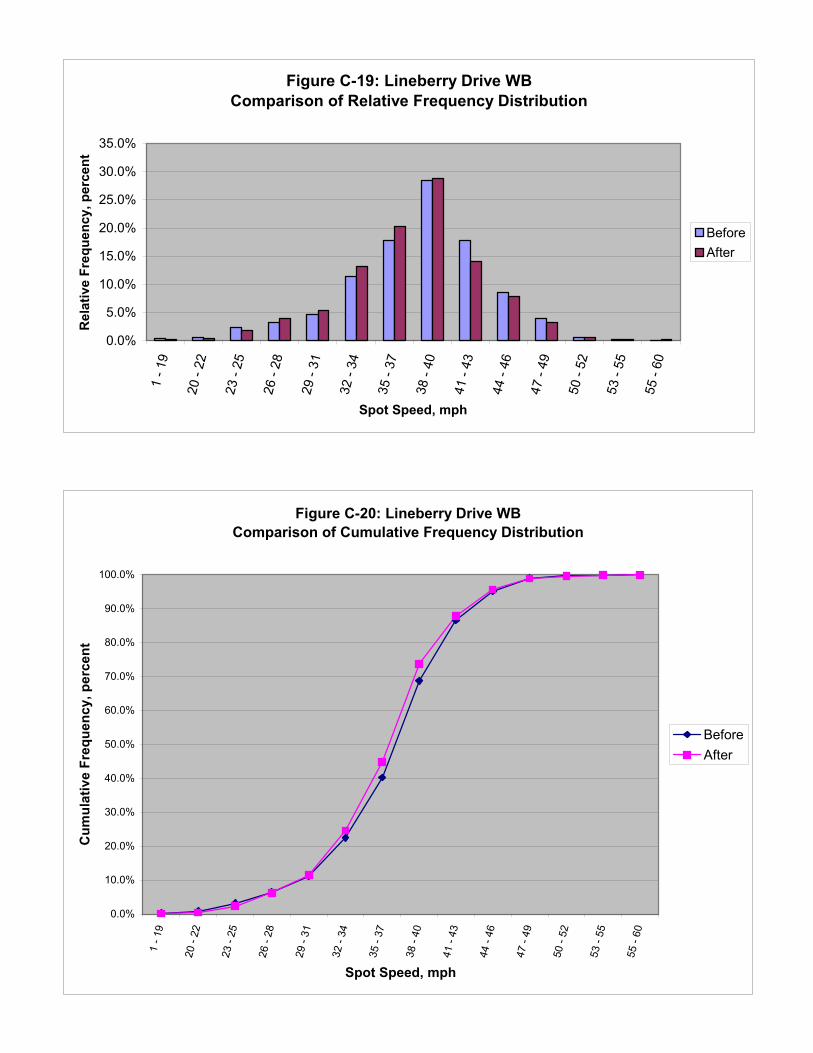
Figure C-19: Lineberry Drive WBComparison of Relative Frequency Distribution

0.0%

5.0%

10.0%

15.0%

20.0%

25.0%

30.0%

35.0%1

- 19

20 -

22

23 -

25

26 -

28

29 -

31

32 -

34

35 -

37

38 -

40

41 -

43

44 -

46

47 -

49

50 -

52

53 -

55

55 -

60

Spot Speed, mph

Rel

ativ

e Fr

eque

ncy,

per

cent

BeforeAfter

Figure C-20: Lineberry Drive WBComparison of Cumulative Frequency Distribution

0.0%

10.0%

20.0%

30.0%

40.0%

50.0%

60.0%

70.0%

80.0%

90.0%

100.0%

1 - 1

9

20 -

22

23 -

25

26 -

28

29 -

31

32 -

34

35 -

37

38 -

40

41 -

43

44 -

46

47 -

49

50 -

52

53 -

55

55 -

60

Spot Speed, mph

Cum

ulat

ive

Freq

uenc

y, p

erce

nt

BeforeAfter

Documents

An Evaluation of Edge Line Striping as a Traffic Calming Technique … · 2008-05-24 · Edge Line Striping as a Traffic Calming Technique Eric J. Lamb, PE January 13, ... The researcher