Embed Size (px)
Citation preview
Univers
ity of
Cap
e Tow
n
AN EXPERIMENTAL INVESTIGATION INTO TRE COMPONENTS
OF SHIP RESISTANCE
I
by
Robert Cooke, B.Sc. (Civil) Engineering, Cape Town
A thesis submitted in partial fulfilment of the
requirements for the degree Master of Science in
Engineering
Department of Civil Engineering
University of Cape Town
September 1986

The copyright of this thesis vests in the author. No quotation from it or information derived from it is to be published without full acknowledgement of the source. The thesis is to be used for private study or non-commercial research purposes only.
Published by the University of Cape Town (UCT) in terms of the non-exclusive license granted to UCT by the author.
Univers
ity of
Cap
e Tow
n

Univers
ity of
Cap
e Tow
n
i
To my Dad
Univers
ity of
Cap
e Tow
n
DECLARATION OF CANDIDATE
I, Robert Cooke, hereby declare that this thesis is my own
work and that it has not been submitted for a degree at
another university.
ii
R COOKE
September 1986
Univers
ity of
Cap
e Tow
n
SYNOPSIS
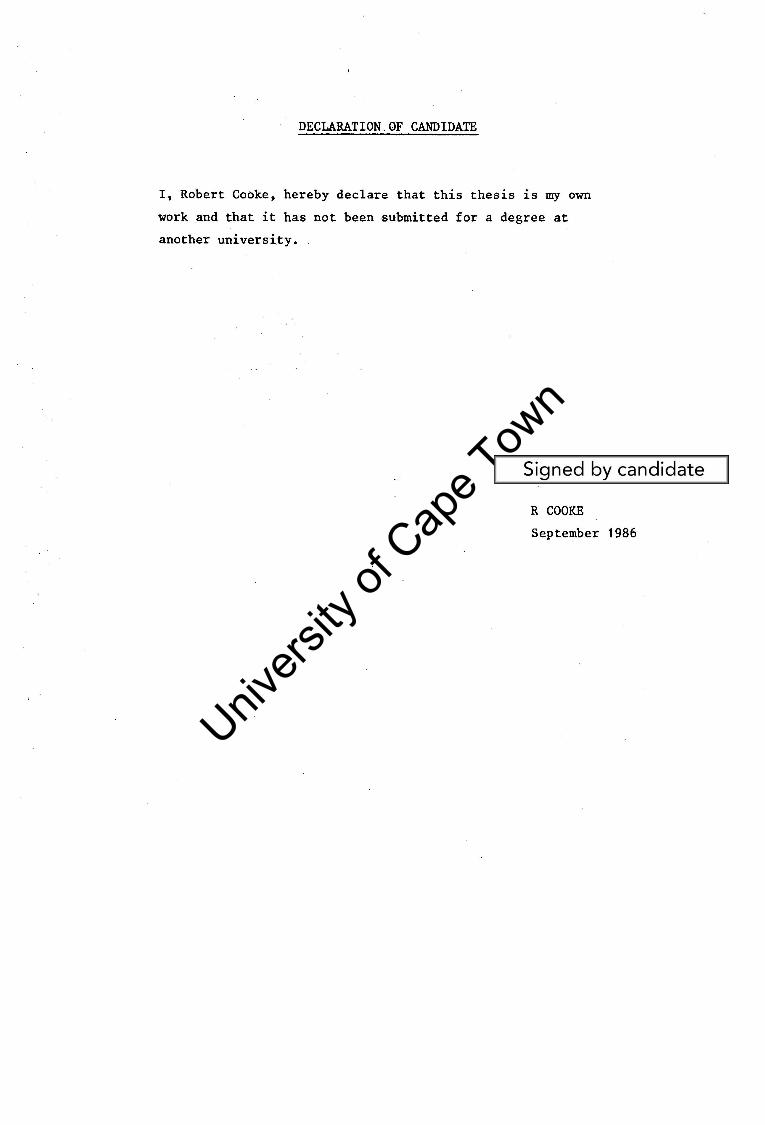
This thesis is an experimental investigation into the components of
ship resistance. The traditional Froude method of scaling .is investi
gated with reference to the measurement of skin friction and viscous
pressure resistance. A literature review is given on the theoretical
background and experimental measurement techniques.
Two models are used for the experimental work, which sizes are in the
geometric ratio of 2,7 to 1. The model form is half .a body of revolu
tion with a vertical sided superstructure. The block coefficient of
the model is 0,621 and the length to beam ratio is 7. Two surface
models and one reflex model are tested. One of the models has 40
pressure tappings located_on its hull which are used to measure the
total pressure resistance of the model.
The components of resistance directly measured·are total resistance,
iii
total viscous resistance and total pressure resistance. The resistance
components inferred are skin friction resistance and wave-making resistance.
The.deduced skin friction is found to deviate from the Prandtl-von Karman
skin friction formulation. The wave-making resistance agrees favourably
with the predicted values using Mit.chell 's integral. ·The total viscous
resistance increases sharply at Reynolds numbers greater than 3 x 10⁶•
Univers
ity of
Cap
e Tow
n
ACKNOWLEDGEMENTS
The author wishes to thank the. following:-
Professor F A Kilner, Department of Civil Engineering, U C T, thesis
supervisor, for his insight, guidance and encouragement over the past
two years.
The Council for Scientific and Industrial Research for the award of
a post-graduate grant which made this research possible.
Mr K Balfour, undergraduate student, for his help with the glass flume
experiments.
Messrs R F Beverton, G Bertuzzi, D J Botha, C Coetzee and R Edge of
the Civil Engineering workshop, UC T, for their assistance with the
fabrication of the experimental apparatus.
Mr J J Hesselink, Department of Electrical Engineering, U C T, for
advice.concerning electronic problems and the loan of equipment.
Mr J Mayer., Department of ·Mechanical Engineering, U C T, for the loan
of equipment.
Mr A Sive, Department of Civil Engineering, UC T, for the many
enlightening discussions.
Messrs J H George, N Hassan, J Petersen, A Siko, D S Swart and
J J Williams of the Department of Civil Engineering, UC T, for the
assistance and encouragement throughout the thesis.
Cheryl Wright for her efficient typing of this thesis.
iv
Univers
ity of
Cap
e Tow
n
DECLARATION
SYNOPSIS
ACKNOWLEDGEMENTS
TABLE OF CONTENTS
LIST OF FIGURES
LIST OF TABLES
TABLE OF CONTENTS
LIST OF PHOTOGRAPHIC PLATES
NOMENCLATURE
CO-ORDINATE SYSTEM
1.
2.
INTRODUCTION
THEORETICAL BACKGROUND
2. 1 Definitions
2.1.1 Reynolds number
2.1.2 Froude number
2.2 The nature of ship resistance
2 .2. 1 Resistance in an ideal fluid
2.2.1.1 Model submerged
2.2.1.2 Model at the surface
2.2.2 Resistance in a viscous fluid
2.2.2.1 Model submerged
2.2.2.2 Model at the surface
v
ii
iii
iv
v
x
xiii
xiv
xv
xviii
1. 1
2. 1
2. 1
2. 1
2. 1
2.2
2.3
2.3
2.4
2.4
2.4
2.5
Univers
ity of
Cap
e Tow
n
3.
2.3
2.4
2.5
2.6
Modelling ship resistance
2.3.1
2.3.2
2.3.3
2.3.4
Dimensional analysis for a surface body
Scaling from model to prototype
Froude's method
Extension of model resistance to prototype
resistance
Skin friction
2. 4. 1 Skin friction acting on a flat plate
vi
2.8
2.8
2 .10
2. 12
2. 14
2. 16
2. 17
2. 4. 1 • 1 Laminar boundary layer 2. 22
2.4.1.2 Turbulent boundary layer on a
smooth flat plate 2. 25
2.4.1.3 Laminar and turbulent flow on a
. smooth flat plate 2. 29
2.4.1.4 Turbulent flow on. a rough flat plate 2.30
2.4.2 Skin friction acting on a ship 2.32
Viscous pressure resistance 2.35
Wave-making resistance
2. 6. 1
2.6.2
2.6.3
The nature of wave-making resistance
Theoretical calculation of wave-making resistance
"Humps and hollows" in resistance curves
2.36
2.36
2.40
2.42
EXPERIMENTAL MEASUREMENT TECHNIQUES 3. 1
3. 1 Total resistance 3. 1
3.2 Total viscous resistance 3.3
Univers
ity of
Cap
e Tow
n 4.
5.
3.3 Skin friction
3.3.1 Direct measurements
3.3.2 Stanton gauge
3.3.3 Preston tube
3.3.4 Thin film probes
3.4 Total pressure resistance
3.5 Wave-making resistance
EXPERIMENTAL OBJECTIVES
4. 1 Objectives
4.2 Choice of model form
GLASS FLUME EXPERIMENT.
5. 1
5.2
5.3
5.4
Glass flume
Model ship
Measurement of water speed in the flume
Measurement of total resistance
5. 4. 1
5.4.2
5.4.3
5.4.4
Alternative model support methods
Alternative load sensing devices
Choice of measurement system
Fabrication of total resistance measurement
system
5.4.4.1
5.4.4.2
5.4.4.3
Air tracks
Model support
Cantilever resistance measuring device
vii
3.5
3.5
3.6
3.7
3.9
3 .10
3. 11
4. 1
4. 1
4.2
5. 1
5. 1
5.3
5.5
5.5
5.7
5.9
5. 11
5.12
5. 12
5. 15
5. 15
Univers
ity of
Cap
e Tow
n 6.
5.5
5.4.5 Experimental procedure
5.4.5.1
5.4.5.2
Calibration-of strain gauge bridge
Total resistance measurement procedure
Measurement of total pressure resistance
5. 5. 1
5.5.2
5.5.3
. 5.5.4
5.5.5
Alternative methods of measuring pressure
Choice of pressure measurement method
Fabrication of the manometer board
Experimental procedure
Calculation of total pressure resistance
TOWING CHANNEL EXPERIMENT
6. 1 Towing trolley and channel
6. 2 . Model
6.3
6.4
Measurement of trolley speed
Measurement of total resistance
6. 4 .1
6.4.2
6.4.3
Total resistance measurement system
Fabrication of total.resistance measurement system
6.4.2.1
6.4.2.2
Support framework
Resistance measuring device
Experimental procedure
viii
5 .17
5 .17
5. 19
5.22
5.22
5.23
5.23
5.25
5.28
6. 1
6.2
6.2
6.6
6.6
6.8
6.8
6 .10
6. 13

Univers
ity of
Cap
e Tow
n
7.
8.
DISCUSSION AND PRESENTATION OF RESULTS
7 .1 Glass flume experimental results
7.2 Towing channel experimental results
7.3 Comparison between glass flume and, towing channel
experimental results
CONCLUSIONS
BIBLIOGRAPHY
APPENDICES
A.
B.
c.
D.
Examinations written by the author to complete the require
ments of the degree
Glass flume experiment
B.1 Pressure tapping locations
B.2 Capillary rise in tubes
B.3 Calculation method for total pressure resistance
Low pass filter
Strain gauge bridge theory
ix
7. 1
7. 1
7.7
7.20
8.1
BIB.1
A.1
B .1
B.2
B.4
B.6
c .1
D.1
Univers
ity of
Cap
e Tow
n
2. 1
2.2
2.3
LIST OF FIGURES
Shear stress and normal pressure on a ship hull
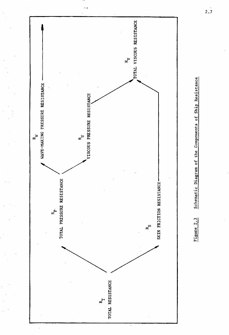
Components of ship resistance
Schematic diagram of components of ship resistance
2.4 Loss in performance with time in service for a cross-
channel ship
2.5 Development of boundary layer on a flat plate
2.6 Streamline afong a flat plate
2.7 Boundary layer velocity distribution
2.8 Flat plate skin friction formulations
2.9 Rough plate skin friction
2.10 Skin friction formulations
2.11 Separation on a ship form
2.12 Kelvin wave pattern
2.13 Froude's original sketch of a bow wave train
2.14 Ship wave pattern
2.15 Dimensionless co-ordinate system
2.16 Characteristic total resistance curve
2.17 Profiles along model's hull
3. 1 Froude's dynamometer
3.2 Flow past a cylinder
3.3 Skin friction gauge
3.4 Stanton gauge
3.5 Preston tube
x
2.2
2.6
2.7
2. 17
2 .18
2.20
2.22
2.24
2.31
2.33
2.35
2.38
2.39
2.40
2.41
2.44
2.44
3.2
3.3
3.6
3.7
3.8
Univers
ity of
Cap
e Tow
n
4.1 Form of models
4.2 Computed wave-making resistance
4.3 Relative dimensions of models
5.1 Recirculating water system
5.2 Pressure tapping locations
5.3 Alternative support methods
5.4 Cantilever load sensing device
5.5 Air track
5.6 Compressor connection to air tracks
5.7 Dual air track model support system
5.8 Strain gauge bridge connection diagram
5.9 Typical strain gauge calibration graph
5.10 Typical total resistance plot
5.11 Model .pressure tapping connection to manometer board
6.1 Typical variation of trolley speed with time
6. 2 Method of obtaining total resistance of .. the submerged model
6.3 Support strut profile
6.4 Typical measurement of total resistance
6.5 Plan view of submerged model and support fins
xi
4.3
4.4
4.5
5.2
5.6
5.8
5 .10
5. 13
5. 14
5 .15
5 .16
5. 19
5.21
5.27
6.5
6.7
6.9
6 .16
6. 18
Univers
ity of
Cap
e Tow
n
7.1 Glass flume model - total resistance and total pressure
resistance
7.2 Glass flume model - computed wave-making resistance
7.3 Glass flume model - resistance coefficients versus
Froude m.unber
7.4 Glass flume model - resistance coefficients versus
Reynolds number
7.2
7.2
7.3
7.3
7.5 Glass flume model - skin friction versus model velocity 7.4
7.6 Glass flume model - skin friction coefficient versus
Reynolds number 7 .4
7.7 Glass flume model - water surface profiles 7.5
7.8 Towing channel model - total resistance of submerged model 7.10
7.9 Towing channel model - viscous resistance of surface model 7.10
7.10 Towing channel model - total viscous resistance coefficient
versus Reynolds number 7.11
7.11 Towing channel model - total viscous resistance coefficient
versus Froude number
7 .12 Towing channel model - measured CV versus calculated CV
by Blevins method
7.13 Towing channel model - comparison of resistance coefficients
of various bodies
7. 14 Towing channel model - resistance components of surface model
7.15 Towing channel model - deduced and calculated wave-making
resistance
7 .16 Towing channel model - total resistance coefficient curve
7.17 Towing channel model - wave-making resistance coefficient
curve
7 .18 Towing channel model - water surface profiles
7.19 Towing channel model - variation of model resistance with
submergence
7.20 Residuary resistance of surface models versus Froude number
7.21 Skin friction and viscous resistance of surface models
7. 11
7 .12
7 .13
7 .14
7 .14
7 .15
7 .15
7. 16
7. 19
7.22
7.23
Univers
ity of
Cap
e Tow
n
xiii
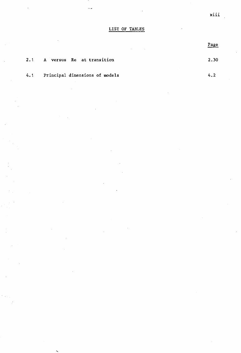
LIST OF TABLES
2. 1 A versus Re at transition 2.30
4. 1 Principal dimensions of models 4.2
Univers
ity of
Cap
e Tow
n
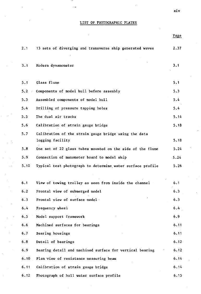
LIST OF- PHOTOGRAPHIC PLATES
2.1 13 sets of diverging and transverse ship generated waves
3.1 Modern dynamometer
5.1 Glass flume
5.2 Components of model hull before assembly
5.3 Assembled components of model hull
5.4 Drilling of pressure tapping holes
5.5 The dual air tracks
5.6 Calibration of strain gauge bridge
5.7 Calibration of the strain gauge bridge using the data
logging facility
5.8 One set of 22 glass tubes mounted on the side of the flume
5.9 Connection of manometer board to model ship
5.10 Typical test photograph to determine. water surface profile
6.1 View of towing trolley as seen from inside the channel
6.2 Frontal view of submerged model
6.3 Frontal view of surface model -
6.4 Frequency wheel
6.5 Model support framework
6.6 Machined surfaces for bearings
6.7 Bearing housings
6.8 Detail of bearings
6.9 Bearing detail and machined surface for vertical bearing
6.10 Plan view of resistance measuring beam
6.11 Calibration of strain gauge bridge
6.12 Photograph of hull water surface profile
xiv
2.37
3. 1
5. 1
5.3
5.4
5.4
5. 14
5 .18
5 .18
5.24
5.24
5.26
6. 1
6.3
6.3
6.4
6.9
6. 11
6. 11
6. 12
6.12
6 .14
6. 14
6.15
Univers
ity of
Cap
e Tow
n
Symbol
b
B
c
c 0
d
D
D
F r
g
k adm
L
p
R
Re z
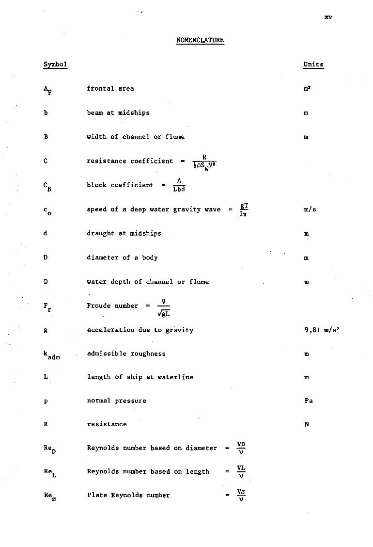
NOMENCLATURE
frontal area
beam at midships
width of channel or flume
resistance coefficient = R
block coefficient =
speed of a deep water gravity wave
draught at midships
diameter of a body
water depth of channel or flume
Froude number v = /gL
acceleration due to gravity
admissible roughness
length of ship at waterline
normal pressure
resistance
Reynolds number based on diameter
Reynolds number based on length
Plate Reynolds number
=
=
=
VD v
VL v
Vz v
xv
Units
m2
m
m
m/s
m
m
m
9,81 m/s2
m
m
Pa
N
Univers
ity of
Cap
e Tow
n
Symbol
s
T
v
x
y
z
A 0
µ
\)
p
l" 0
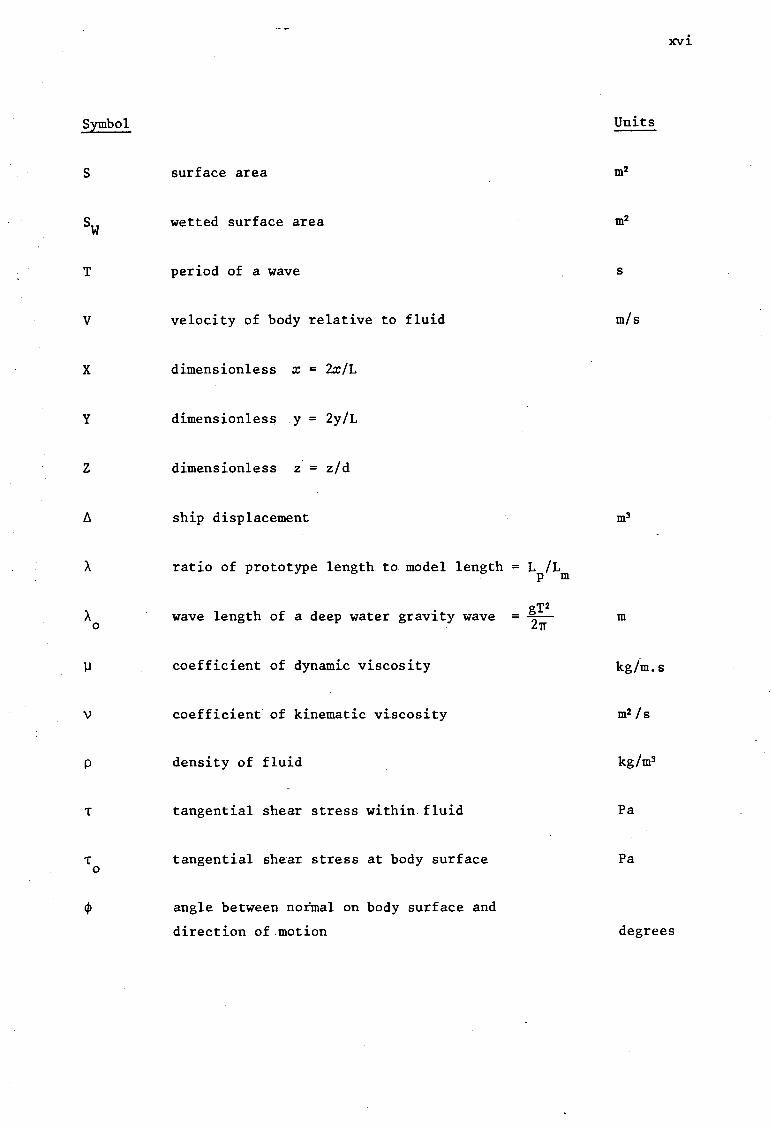
surf ace area
wetted surface area
period of a wave
velocity of body relative to fluid
dimensionless x = 2.x/L
dimensionless y = 2y/L
dimensionless z = z/d
ship displacement
ratio of prototype length to model length = L /L p m
-- gT2 wave length of a deep water gravity wave 21T
coefficient of dynamic viscosity
coefficient of kinematic viscosity
density of fluid
tangential shear stress within fluid
tangential shear stress at body surface
angle between normal on body surf ace and
direction of motion
xvi
Units
m2
m2
s
m/s
m3
m
kg/m. s
m2 /s
kg/m3
Pa
Pa
degrees
Univers
ity of
Cap
e Tow
n
xvii
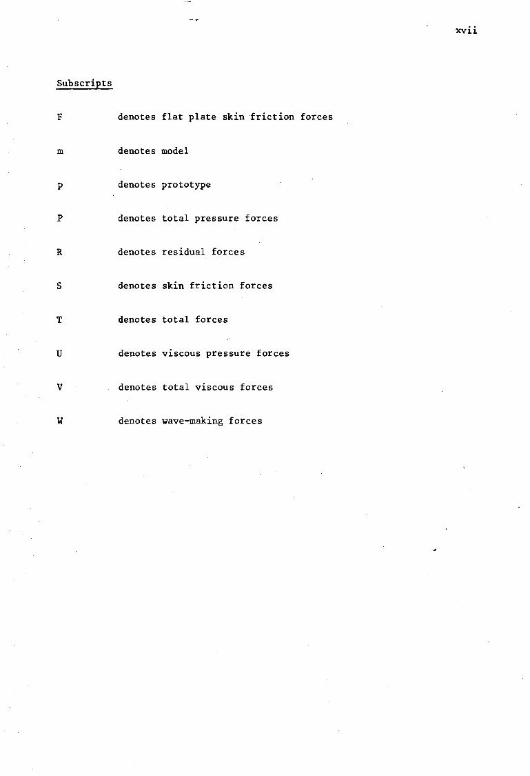
Subscripts
F denotes flat plate skin friction forces
m denotes model
p denotes prototype
p denotes total pressure forces
R denotes residual forces
s denotes skin friction forces
T denotes total forces
u denotes viscous pressure forces
v denotes total viscous forces
w denotes wave-making forces
...
Univers
ity of
Cap
e Tow
n
xviii
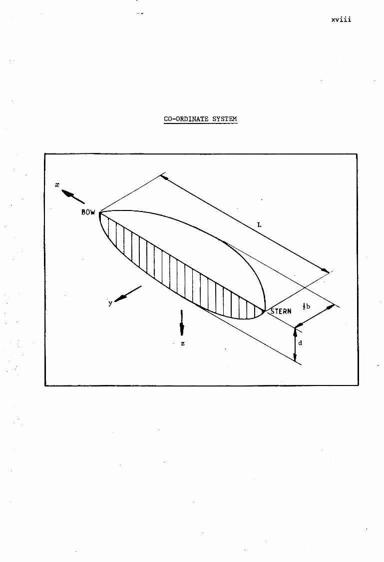
CO-ORDINATE SYSTEM
y /
z
Univers
ity of
Cap
e Tow
n
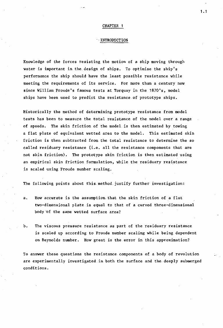
CHAPTER 1
· · INTRODUCTION
Knowledge of the forces resisting the motion of a ship moving through
water is important in the design of ships. To optimise the ship's
performance the ship should have the.least possible resistance while
meeting the requirements of its service. For more than a century now
since William Froude's famous tests at Torquay in the 1870's, model
ships have been used to predict the resistance of prototype ships.
Historically the method of determining prototype resistance from model
tests has been to measure the total resistance of the model over a range
of speeds. The skin friction of the model is then estimated by towing
a flat plate of equivalent wetted area to the model. This estimated skin
friction is then subtracted from the total resistance to determine the so
called residuary resistance (i.e. all the resistance components that are
not skin friction). The prototype skin friction is then estimated using
an empirical skin friction formulation, while the residuary resistance
is scaled using Froude number scaling.
The following points about this method justify further investigation:
a. How accurate is the assumption that the skin friction of a flat
two-dimensional plate is equal to that of a curved three-dimensional
body 'of the same wetted surface area?
b. The viscous pressure resistance as part of the residuary resistance
is scaled up according to Froude number scaling while being dependent
on Reynolds number. How great is the error in this approximation?
1. 1
To answer these questions the resistance components of a body of revolution
are experimentally investigated in both the surface and the deeply submerged
conditions.
Univers
ity of
Cap
e Tow
n
2. 1
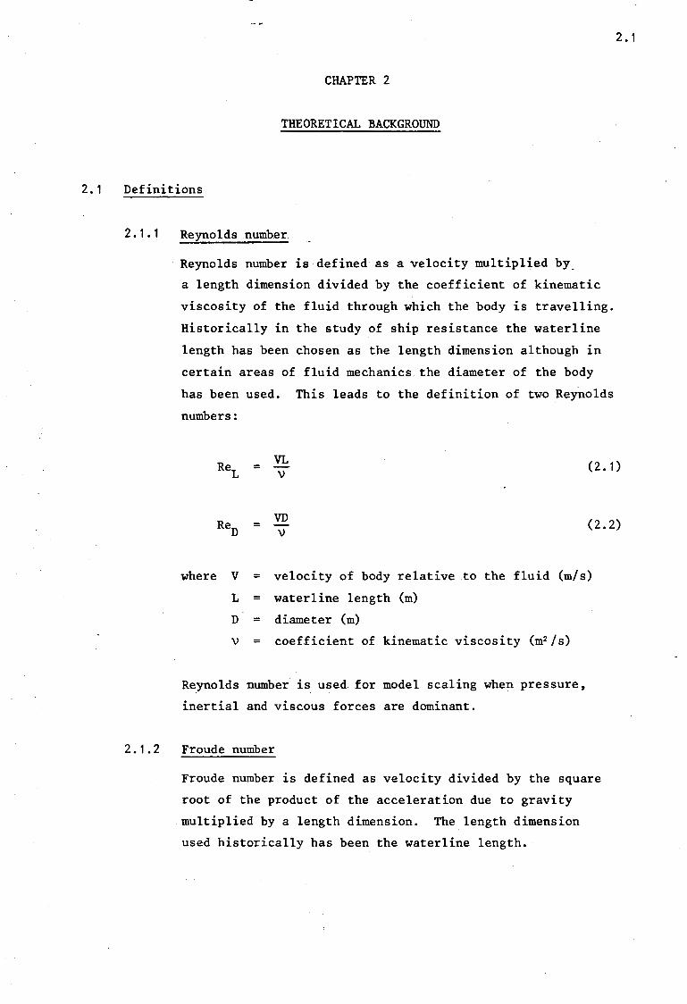
CHAPTER 2
THEORETICAL BACKGROUND
2.1 Definitions
2 .1.1
2. 1 • 2
Reynolds number.
Reynolds number is defined as a velocity multiplied by_
a length dimension divided by the coefficient of kinematic
viscosity of the fluid through which the body is travelling.
Historically in the study of ship resistance the waterline
length has been chosen as the length dimension although in
certain areas of fluid mechanics the diameter of the body
has been used. This leads to the definition of two Reynolds
numbers:
ReL VL = \)
(2 .1)
ReD VD = \)
(2.2)
where v = velocity of body relative to the fluid (m/s)
L = waterline length (m)
D = diameter (m)
\) = coefficient of kinematic viscosity (m2 Is)
Reynolds number is used for model scaling when pressure,
inertial and viscous forces are dominant.
Froude number
Froude number is defined as velocity divided by the square
root of the product of the acceleration due to gravity
multiplied by a length dimension. The length dimension
used historically has been the waterline length.
Univers
ity of
Cap
e Tow
n
2.2
Thus v = (2.3) lgL
where g = acceleration due to gravity (m/s2 )
Froude number model scaling is used when pressure, inertial
and gravity forces are dominant.
2.2 The nature of ship resistance
In fluid mechanics the term resistance is the retarding force
experienced by a body when moving through a fluid. In aerodynamics
this retarding force is generally.called drag; however, naval
architects have historically referred to it as resistance. Resistance
is found in all situations where a real fluid moves relative to a
body e.g. pipe flow, open channel flow and, of more specific interest,
the resistance of the sea opposing the motion of a ship's hull.
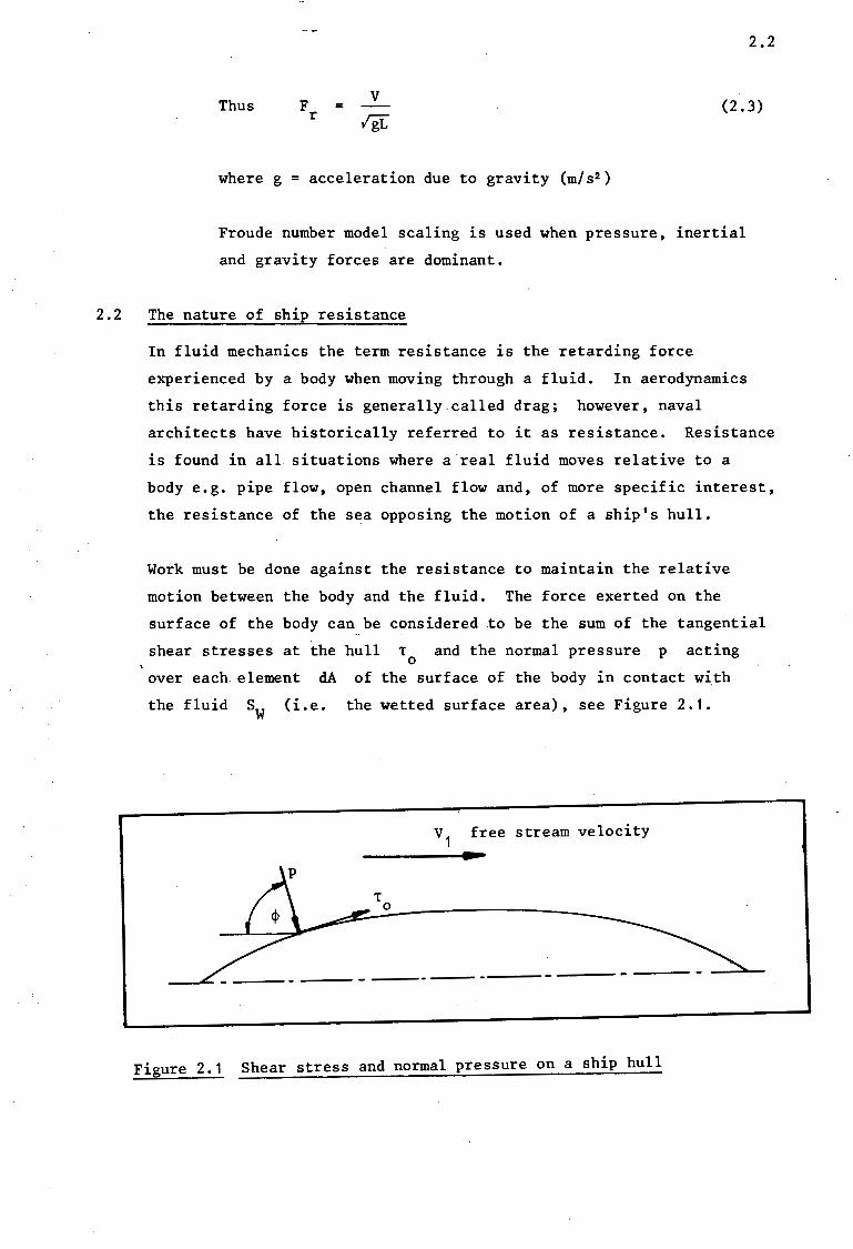
Work must be done against the resistance to maintain the relative
motion between the body and the fluid. The force exerted on the
surface of the body can be considered to be the sum of the tangential
shear stresses at the hull T and the normal pressure p acting 0
over each element dA of the surface of the body in contact with
the fluid SW (i.e. the wetted surface area), see Figure 2.1.
v1 free stream velocity -
Figure 2.1 Shear stress and normal pressure on a ship hull
Univers
ity of
Cap
e Tow
n
= T sin¢ dA 0
+ f 5 p cos¢ dA w
2.3
(2.4)
where Rr = total resistance (N)
¢ = angle between surface dA and direction of motion.
The first term on the righthand side of this equation is termed
skin friction and is .the longitudinal resultant of viscous shear
forces of the fluid against the hull surface. The second term on
the righthand side of the equation is called the total pressure
resistance and is the longitudinal resultant of the normal pressures
exerted at the surface.
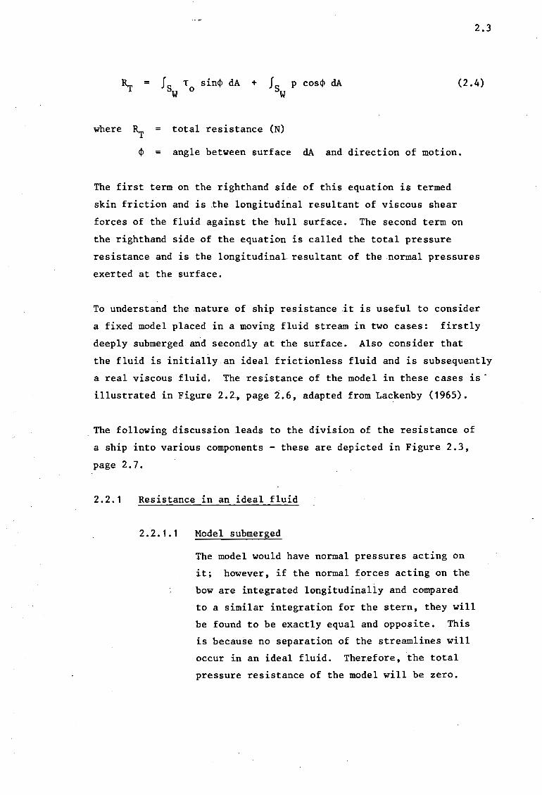
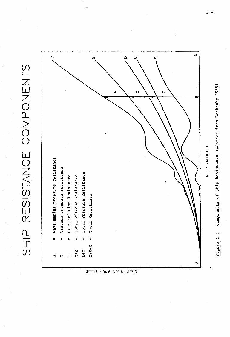
To understand the nature of ship resistance it is useful to consider
a fixed model placed in a moving fluid stream in two cases: firstly
deeply submerged and secondly at the surface. Also consider that
the fluid is initially.an ideal frictionless fluid and is subsequently
a real viscous fluid. The resistance of the model in these cases is ·
illustrated in Figure 2.2, page 2.6, adapted from Lackenby (1965) •
. The following discussion leads to the division of the resistance of
a ship into various components - these are depicted in Figure 2.3,
page 2.7.
2. 2. 1 Resistance in an ideal fluid
2.2.1.1 Model submerged
The model would have normal pressures acting on
it; however, if the normal forces acting on the
bow are integrated longitudinally and compared
to a similar integration for the stern, they will
be found to be exactly equal and opposite. This
is because no separation of the streamlines will
occur in an ideal fluid. Therefore, the total
pressure resistance of the model will be zero.

Univers
ity of
Cap
e Tow
n
2.2.2
2.2.1.2
Similarly, there would be no tangential shear
stresses acting on the model in this case.
Thus the model would have zero resistance and
this is represented as line OA in Figure 2.2.
Model at the surface
The model would generate a set of gravity waves
in the fluid stream as it flowed past the model.
The generation of the gravity waves would be
seen at the hull of the model as normal pressures.
The longitudinal integrated normal pressure forces
would, therefore, be non-zero and equal to the
theoretical wave-making resistance of the form.
This is depicted as curve OB in Figure 2.2.
As the model is in an ideal fluid there would be
no tangential shear stresses acting on the ship.
2.4
Resistance in a viscous fluid
2.2.2.1 Model submerged
Consider firstly the form of the model to be
pressed out into a.thin plate of the same length
and wetted area as the model. Assume that the
plate is infinitely thin so that when the fluid
flows parallel to its plane there are no frontal
pressures acting on the plate; however, tangential
shear stresses will act on the plate due to the
viscosity of the fluid. If these tangential shear
stress forces are integrated longitudinally they
would represent the flat plate skin friction shown
as curve OC in Figure 2.2.
Consider again the three-dimensional body placed in
a moving stream of viscous fluid. · ·rf the tangential
shear stresses acting on the model are integrated
longitudinally the answer will be the real skin
Univers
ity of
Cap
e Tow
n
2.2.2.2
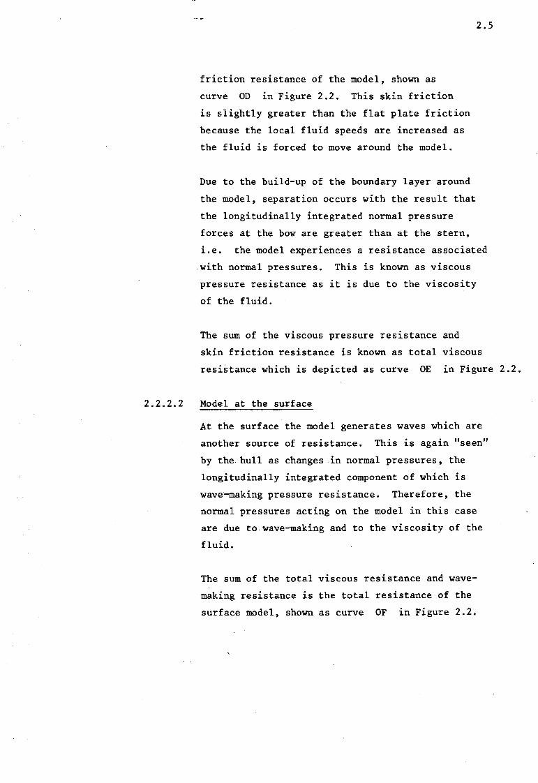
friction resistance of the model, shown as
curve OD in Figure 2.2. This skin friction
is slightly greater than the flat plate friction
because the local fluid speeds are increased as
the fluid is forced to move around the model.
2.5
Due to the build-up of the boundary layer around
the model, separation occurs with the result that
the longitudinally integrated normal pressure
forces at the bow are greater than at the stern,
i.e. the model experiences a resistance associated
with normal pressures. This is known as viscous
pressure resistance as it is due to the viscosity
of the fluid.
The sum of the viscous pressure resistance and
skin friction resistance is known as total viscous
resistance which is depicted as curve OE in Figure 2.2.
Model at the surface
At the surface the model generates waves which are
another source of resistance. This is again "seen"
by the hull as changes in normal pressures, the
longitudinally integrated component of which is
wave4naking pressure resistance. Therefore, the
normal pressures acting on the model in this case
are due to wave-making and to the viscosity of the
fluid.
The sum of the total viscous resistance and wave
making resistance is the total resistance of the
surface model, shown as curve OF in Figure 2.2.
Univers
ity of
Cap
e Tow
n
SH
IP
RE
SIS
-rA
NC
E
x =
W
ave
mak
ing
pre
ssu
re re
sist
an
ce
Y
=
Vis
cous
p
ress
ure
re
sist
an
ce
Z
=
Sk
in F
ricti
on
Res
ista
nce
Y+Z
=
T
ota
l V
isco
us
Res
ista
nce
X+Y
=
To
tal
Pre
ssu
re R
esis
tan
ce
~
~ I
X+Y
+Z
=
To
tal
Res
ista
nce
0 ~
~
u ~ H
00
H
0
0
~ tl.<
H ~
0
SHIP
VEL
OCI
TY C
OM
PO
NE
NT
S
Fig
ure
2.2
C
ompo
nent
s o
f S
hip
Res
ista
nce
(a
dap
ted
fro
m L
acke
nby
1965
)
F
D c B A
"" 0\
Univers
ity of
Cap
e Tow
n
~
~
I W
AVE-
MAK
ING
PRES
SURE
RE
SIST
AN
CE ----------
TOTA
L PR
ESSU
RE
RESI
STA
NCE
l\r
VIS
COU
S PR
ESSU
RE
RESI
STA
NCE
Rr
TOTA
L RE
SIST
AN
CE
~
TOTA
L V
ISCO
US
SKIN
FR
ICTI
ON
RE
SIST
AN
CE
~ RE
SIST
AN
CE
RS
Fig
ure
2.3
S
chem
atic
Dia
gram
of
the
Com
pone
nts
of
Shi
p R
esis
tan
ce
N . -...J
Univers
ity of
Cap
e Tow
n
2.8
2.3 Modelling ship resistance
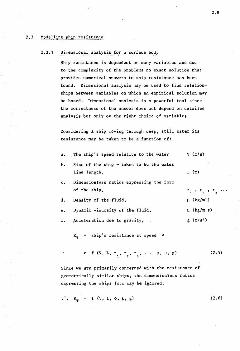
2. 3. 1 Dimensional analysis for a surface body
Ship resistance is dependent on many variables and due
to the complexity of the problems no exact solution that
provides numerical answers to ship resistance has been
found. Dimensional analysis may be used to find relation
ships between variables on which an empirical solution may
be based. Dimensional analysis is a powerful tool since
the correctness of the answer does not depend on detailed
analysis but only on the right choice of variables.
Considering a ship moving through deep, still water its
resistance may be taken to be a function of:
a. The ship's speed relative to the water
b. Size of the ship - taken to be the water
line length,
V (m/s)
L (m)
c. Dimensionless ratios expressing the form
of the ship, r , r , r 1 2 3
d.
e.
f.
Density of the-fluid,
Dynamic viscosity of the fluid,
Acceleration due to gravity,
= ship's resistance at speed v
= f (V, L, r,r,r, l 2 3
••• ' p, µ' g)
p (kg/m3 )
µ (kg/m. s)
g (m/s2 )
(2.5)
Since we are primarily concerned with the resistance of
geometrically similar ships, the dimensionless ratios
expressing the ships form may be ignored.
= f (V, L, p, µ, g) (2.6)
Univers
ity of
Cap
e Tow
n
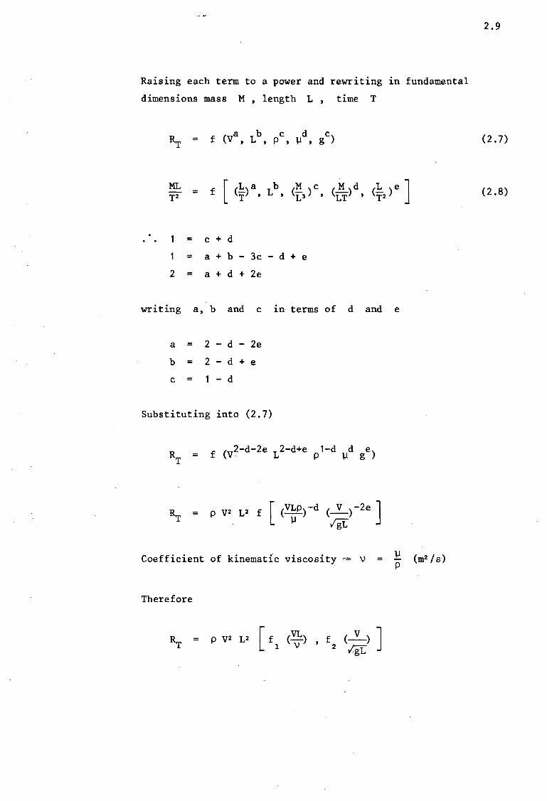
Raising each term to a power and rewriting in fundamental
dimensions mass M , length L , time T
= c + d
= a + b - 3c - d + e
2 = a + d + 2e
writing a, b and c in terms of
a = 2 - d - 2e
b = 2 - d + e
c = - d
Substituting into (2.7)
f 2-d-2e 2-d+e 1-d RT = (V L p
d and
d ge) µ
~ = P v2_ L2 f [ (VLP) -d (~) -2e J µ ;gr:-
Coefficient of kinemat1c viscosity ~= v =
Therefore
= P V2 L2 [ f ( VL) f ·. l \) ' 2
e
µ p
(m2 Is)
2.9
(2.7)
(2.8)
Univers
ity of
Cap
e Tow
n
2.3.2
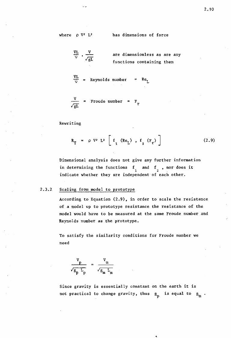
where p v2 L2 has dimensions of force
VL \)
VL \)
v lg[
Rewriting
v lg[
are dimensionless as are any
functions containing them
=
=
=
Reynolds number
Froude number
=
= F r
Dimensional analysis does not give any further information
in determining the functions f and f , nor does it 1 2
indicate whether they are independent of each other.
Scaling from model to prototype
2 .10
(2.9)
According to Equation (2.9), in order to scale the resistance
of a model up to prototype resistance the resistance of the
model would have to be measured at the same Froude number and
Reynolds number as the prototype.
To satisfy the similarity conditions for Froude number we
need
v p
/g L p p
= v
ID
/g L m m
Since gravity is essentially constant on the earth it is
not practical to change gravity, thus gp is equal to g ID
Univers
ity of
Cap
e Tow
n
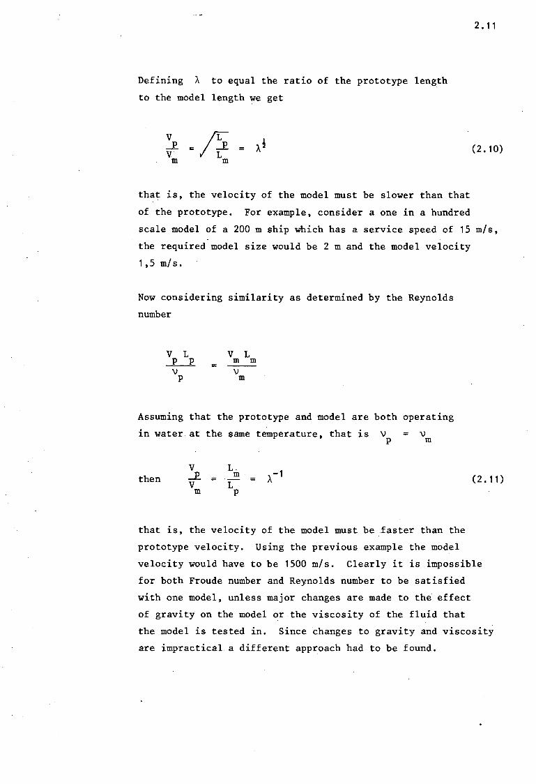
Defining A to equal the ratio of the prototype length
to the model length we get
that is, the velocity of the model must be slower than that
2. 11
(2.10)
of the prototype. For example, consider a one in a hundred
scale model of a 200 m ship which has a service speed of 15 m/s,
the required model size would be 2 m and the model velocity
1,5 m/s.
Now considering similarity as determined by the Reynolds
number
V L p p \)
p =
V L m m \)
m
Assuming that the prototype and model are both operating
in water at the same temperature, that is v = v p m
then v _£. = v
m
Lm
L p
= -1
A (2. 11)
that is, the velocity of the model must be faster than the
prototype velocity. Using the previous example the model
velocity would have to be 1500 m/s. Clearly it is impossible
for both Froude number and Reynolds number to be satisfied
with one model, unless major changes are made to the effect
of gravity on the model or the viscosity of the fluid that
the model is tested in. Since changes to gravity and viscosity
are impractical a different approach had to be found.
Univers
ity of
Cap
e Tow
n
2.3.3
In Equation (2.9) there are the two important dimensionless
ratios; Froude number and Reynolds number. Since Froude
number contains g it can be reasonably expected that
Froude number represents the wave-making resistance of the
ship. Reynolds number contains viscosity and is, therefore,
expected to represent the viscous resistance of the ship.
Froude's method
2. 12
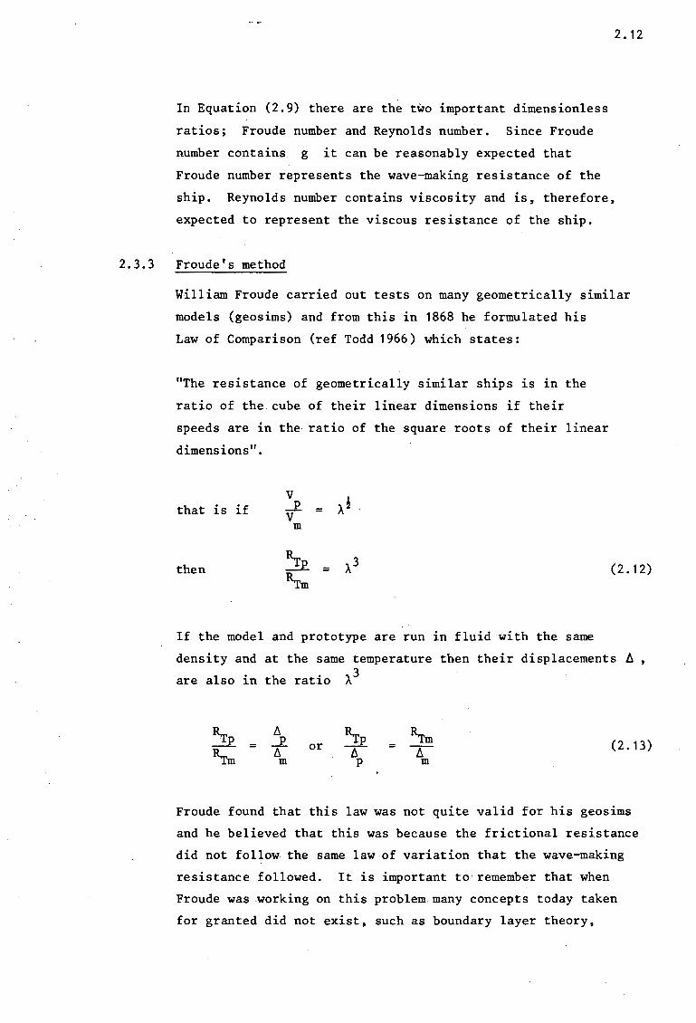
William Froude carried out tests on many geometrically similar
models (geosims) and from this in 1868 he formulated his
Law of Comparison (ref Todd 1966) which states:
"The resistance of geometrically similar ships is in the
ratio of the cube of their linear dimensions if their
speeds are in the ratio of the square roots of their linear
dimensions".
that is if v
Ai __£_ = v m
~ = A3 ~
then (2.12)
If the model and prototype are run in fluid with the same
density and at the same temperature then their displacements ~ ,
are also in the ratio J. 3
= or ~p T
p = (2.13)
Froude found that this law was not quite valid for his geosims
and he believed that this was because the frictional resistance
did not follow the same law of variation that the wave-making
resistance followed. It is important to remember that when
Froude was working on this problem many concepts today taken
for granted did not exist, such as boundary layer theory,
Univers
ity of
Cap
e Tow
n
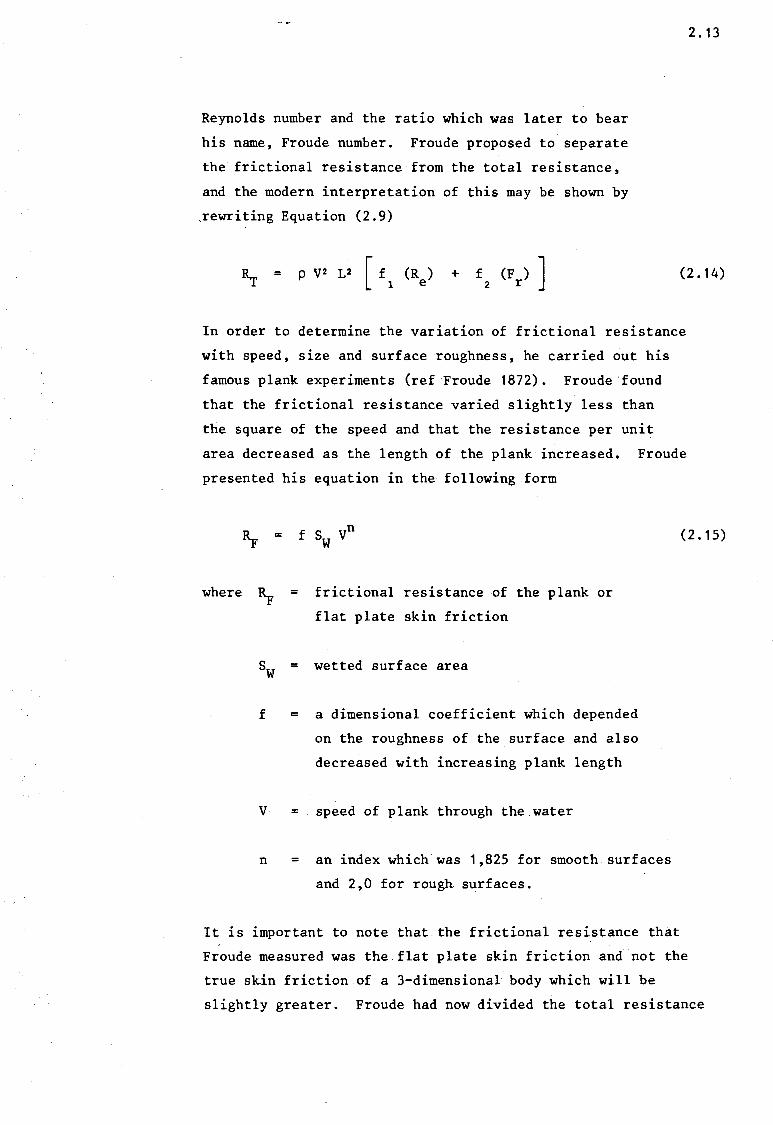
Reynolds number and the ratio which was later to bear
his name, Froude number. Froude proposed to separate
the frictional resistance from the total resistance,
and the modern interpretation of this may be shown by
,rewriting Equation (2.9)
2. 13
= p V2 L2 [ f (R ) 1 e
+ f (F ) J 2 r
(2 .14)
In order to determine the variation of frictional resistance
with speed, size and surface roughness, he carried out his
famous plank experiments (ref Froude 1872). Froude found
that the frictional resistance varied slightly less than
the square of the speed and that the resistance per unit
area decreased as the length of the plank increased. Froude
presented his equation in the following form
=
where ~ = frictional resistance of the plank or
flat plate skin friction
SW = wetted surface area
f = a dimensional coefficient which depended
on the roughness of the surface and also
decreased with increasing plank length
V = speed of plank through the water
n = an index which was 1,825 for smooth surfaces
and 2,0 for rough surfaces.
(2.15)
It is important to note that.the frictional resistance that
Froude measured was the flat plate skin friction and not the
true skin friction of a 3-dimensional body which will be
slightly greater. Froude had now divided the total resistance
Univers
ity of
Cap
e Tow
n
2.3.4
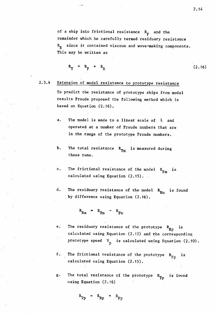
of a ship into frictional resistance ~ and the
remainder which he carefully termed residuary resistance
~ since it contained viscous and wave-making components.
This may be written as
= +
Extension of model resistance to prototype resistance
To predict the resistance of prototype ships from model
results Froude proposed the following method which is
based.on Equation (2.16).
a. The model is made to.a linear scale of A and
operated at a number of Froude·numbers that are
in .the range of the prototype Froude numbers.
b. The total resistance Rrm is measured during
these runs.
c. The frictional resistance of the model ~ni calculat.ed using Equation (2.15).
is
d. The residuary resistance of the model ~ l.S
by difference using Equation (2.16).
found
e. The residuary resistance of the prototype ~p is
calculated using Equation (2.12) and the corresponding
2. 14
(2.16)
prototype speed v p
is calculated using Equation (2.10).
f. The frictional resistance of the prototype ~p l.S
calculated using Equation (2.15).
g. The total resistance of the prototype R.rp l.S found
using Equation (2.16)
ll.rp = ~p + ~p
Univers
ity of
Cap
e Tow
n
This method is the basis of predicting prototype resistance
that is still used in all towing tanks today. There are a
number of new frictional resistance formulations which will
be discussed in Section 2.4.
In order to obtain dimensionless plots of resistance versus
speed various resistance coefficients have.been defined as
follows
2. 15
CT = Total resistance coefficient Rr ;=
(2.17) ! p v2 SW
CF Frictional resistance coefficient ~ = = I P v2 SW (2.18)
CR Residuary resistance coefficient ~ = = ! P v2 SW (2. 19)
The frictional resistance coefficient is generally plotted
against Reynolds number while the residuary resistance
coefficient is plotted against Froude number.
It is important to note that there is an inaccuracy in the
Froude method in that the residuary resistance contains
components (viscous pressure resistance and an extra frictional
force due to curvature) that are dependent on viscosity. These
parts of the residuary resistance are scaled up with the wave
making resistance using Froude number scaling although they
should be scaled using Reynolds number. Nevertheless this
inaccuracy does not seem to have had a major influence on
the results since the Froude scaling method has been used
successfully for nearly a century. It does, however, represent
an area where a refinement of the scaling me.thod could be made.
Univers
ity of
Cap
e Tow
n
2.4 Skin friction
Skin friction is a very important part of ship resistance since
for most ships it is the major component of resistance. On cargo
carriers, which form the major part of the world's mercantile
2. 16
fleet, skin friction can amount up to 85-90% of the total resistance.
Even on higher speed passenger liners and warships where wave
making resistance becomes more influential, skin friction can
account for up to 50% of the total resistance (ref Blevins 1984).
Skin friction also plays an important role in the modelling of ship
resistance. The flow regime around all prototype ships is turbulent
and when a model is tested care must be taken.to ensure that flow
around the model is turbulent (ref Allan and Conn 1950).
If results taken from a model which has been tested in laminar flow
are extrapolated to full scale, the predicted full scale resistance
will be significantly less than the actual resistance of the
prototype.
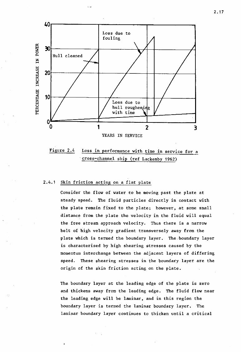
A factor which has a significant effect on skin friction is the
hull surface condition. On clean, new sister ships power differences
of over 20% have been found and this is mainly attributed to dif
ferences in painting and hull surface finish. The change from riveted
.to welded construction has resulted in smoother hulls which give an
estimated power reduction of 20% (ref Lackenby 1962). Corrosion and
fouling of a ship's hull can also significantly affect the ship
resistance. Figure 2.4, page 2.17, shows the increase in power required
by a ship in relation to the number of years in service.
To demonstrate the nature of skin friction it .is useful to consider
a vertical flat plate placed in a moving stream of water. The
resistance acting on the flat plate will be the flat plate skin
friction as discussed in Section 2.2.2.1.
Univers
ity of
Cap
e Tow
n
2. 17
Loss due to fouling
~ 30.--~~~~~----it--~~~~----\~+--+-~~~~~ P.. Hull cleaned z H
r..l
~ 20.--~~~-r--~~t-~~~-r-~~+--+-~~-+-~----'
~ H
due to roughe
with time
oL=====f:::==~==J 0 1 2 3
YEARS IN SERVICE
Figure 2.4 Loss in performance with time .in service for a
· cross-channel ship (ref Lackenby 1962)
2.4.1 Skin friction acting on a flat plate
Consider the flow of water to be moving past the plate at
steady speed. The fluid particles directly in contact with
the plate remain fixed to the plate; however, at some small
distance from the plate the velocity in the fluid will equal
the free stream approach velocity. Thus there is a narrow
belt of high velocity gradient transversely away from the
plate which is termed the boundary layer. The boundary layer
is characterised by high shearing stresses caused by the
momentum interchange between the adjacent layers of differing
speed. These shearing stresses in the boundary layer are the
origin of the skin friction acting on the plate.
The boundary layer at the leading edge of the plate is zero
and thickens away from the leading edge. The fluid flow near
the leading edge will be laminar, and in this region the
boundary layer is termed the laminar boundary layer. The
laminar boundary layer continues to thicken until a critical

Univers
ity of
Cap
e Tow
n Laminar
Figure 2.5
value of plate Reynolds number Re is reached at which x the laminar flow breaks down and becomes generally turbulent.
The fluid particles no longer move in streamlines but have
an oscillatory motion about a mean flow path. The boundary
layer becomes much thicker, thus increasing the amount of
water entrained in the boundary layer, leading to a greater
momentum demand and consequently the resistance to motion
increases. Figure 2.5 shows the development of turbulent
flow along a flat plate. Note that in the turbulent flow
regime there is still a laminar sub-layer through which the
final transfer of momentum is made.
Transition Turbulent
Free stream velocity, V
x Laminar sublayer
Development of boundary layer on a flat plate
2. 18
The value of i.e. · the length of the laminar flow regime
beyond the leading edge of the plate, is only influenced by
the level of turbulence in the approaching fluid. The rough
ness of the surface has no effect on the magnitude of ~ •
Univers
ity of
Cap
e Tow
n
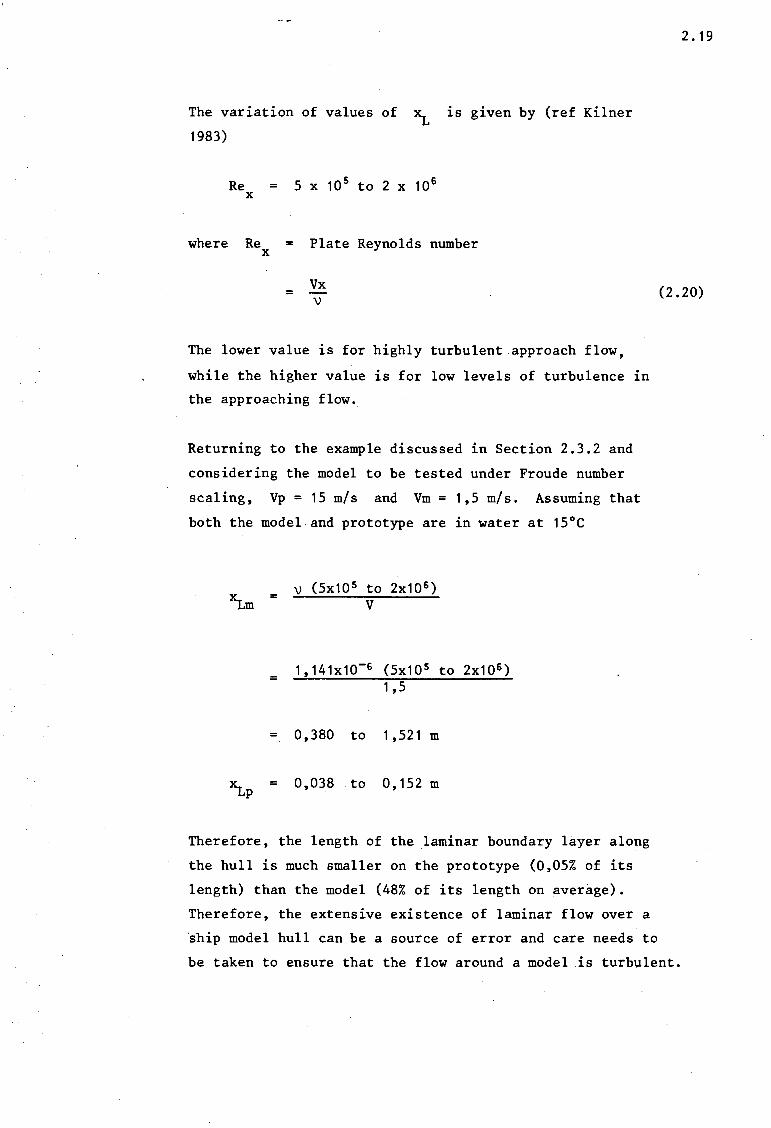
The variation of values of
1983)
Re = 5 x 10 5 to 2 x 10⁶ x
is given by (ref Kilner
where Re = Plate Reynolds number x
2. 19
= Vx \)
(2.20)
The lower value is for highly turbulent approach flow,
while the higher value is for low levels of turbulence in
the approaching flow.
Returning to the example discussed in Section 2.3.2 and
considering the model to be tested under Froude number
scaling, Vp = 15 m/s and Vm = 1,5 m/s. Assuming that
both the model and prototype are in water at 15°C
:l).m =
=
=
:l).p =
v (5x10 5 to 2x10⁶) v
1,141x10-6 (5x10 5
1 '5
0,380 to 1,521 m
0,038 to 0, 152 m
to 2x10⁶)
Therefore, the length of the laminar boundary layer along
the hull is much smaller on the prototype (0,05% of its
length) than the model (48% of its length on average).
Therefore, the extensive existence of laminar flow over a
·ship model hull can be a source of error and care needs to
be taken to ensure that the flow around a model is turbulent.
Univers
ity of
Cap
e Tow
n
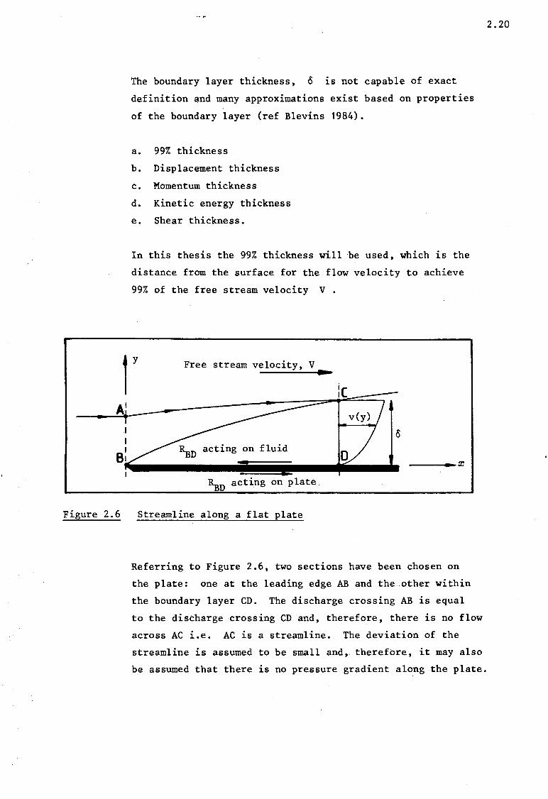
The boundary layer thickness, ~ is not capable of exact
definition and many approximations exist based on properties
of the boundary layer (ref Blevins 1984).
a. 99% thickness
b. Displacement thickness
c. Momentum thickness
d. Kinetic energy thickness
e. Shear thickness.
In this thesis the 99% thickness will be used, which is the
distance from the surface for the flow velocity to achieve
99% of the free stream velocity V •
r Free stream velocity, V .. A'
Figure 2.6
----x ~D acting on plate.
Streamline along a flat plate
Referring to Figure 2.6, two sections have been chosen on
the plate: one at the leading edge AB and the other within
the boundary layer CD. The discharge crossing AB is equal
to the discharge crossing CD and, therefore, there is no flow
across AC i.e. AC is a streamline. The deviation of the
streamline is assumed to be small and,. therefore, it may also
be assumed that there is no pressure gradient along the plate.
2.20
Univers
ity of
Cap
e Tow
n
Thus in applying the impulse momentum principle to ABCD
only the resistance force on the plate and the momentum
pressure forces at AB and CD need to be considered. To
calculate the momentum pressure force at CD the velocity
distribution in the boundary layer must be known. Applying
the impulse momentum principle:
For unit width into the paper
0
2.21
p v2 AB = ~D + f p [v(y)] 2 dy 0
(2. 21)
0 and p V AB = f p v dy
0
from continuity
0 p v2 AB = f p v V dy
0
Equating (2.21) and (2.22)
~D = 0
f (p v V - p v2) dy = 0
0 Pf v (V-v)dy
0
i.e. the resistance acting on a single side of the plate
per unit width. Note that this is a very general result
depending only on velocity distribution at CD and not on
the boundary layer type.
(2. 22)
(2.23)
Univers
ity of
Cap
e Tow
n
-I .§ J!
' l t'· 0 ~
§ .B -' ,..,
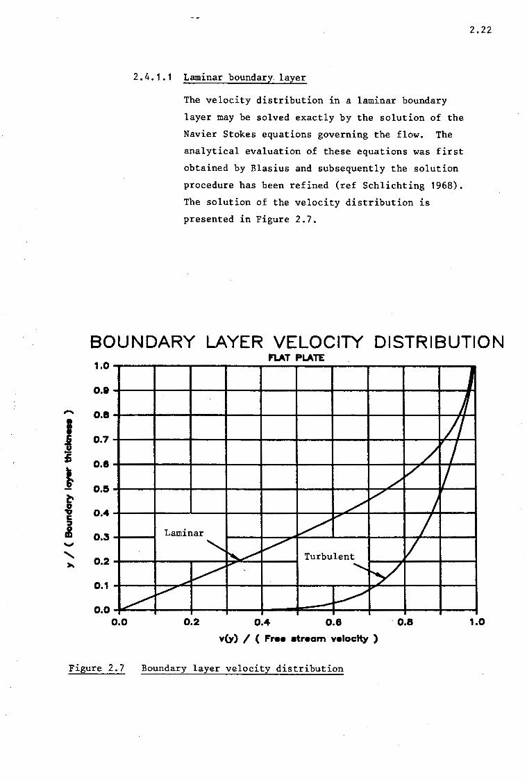
2.4.1.1 Laminar boundary layer
The velocity distribution in a laminar boundary
layer may be solved exactly by the solution of the
Navier Stokes equations governing the flow. The
analytical evaluation of these equations was first
obtained by Blasius and subsequently the solution
procedure has been refined (ref Schlichting 1968).
The solution of the velocity distribution is
presented in Figure 2.7r
2.22
BOUNDARY LAYER VELOCITY DISTRIBUTION 1.0
0.9
o.e
0.7
0.8
o.s
0.4
0.3
0.2
0.1
~ o.o o.o
FLAT PLATE
/ /
/ /
v ~
Laminar
'....... r-...~ ~ v Turbulent
/ ...- ........... y
~
V'" l,_.../ -0.2 0.4 0.8 0.8
v(y) I ( Free etream veloclty )
j
Ii / ~ I
I I
I
1.0
Figure 2.7 Boundary layer velocity distribution

Univers
ity of
Cap
e Tow
n
The thickness of the boundary layer is given
approximately by
2.23
o = 5 fVX = Sx fV = 5x (Re ) -! IV lvx x (2.24)
Thus the boundary layer thickness in laminar flow
increases with the square root of x •
The skin friction acting on the plate may now be
calculated by returning to Equation 2.23 and using
the velocity distribution given in Figure 2.7. The
solution of the integral gives the following
= o, 1328 p v2 o
substituting in Equation 2.24
=
=
0,1328 p v2 Sx (Re)-! x
0,664 p v2 x (Re )-! x
·giving the skin frictional force acting·on one
side of the plate.
The skin frictional resistance coefficient is
= I P v2 x 1,328 (Re)-!
x
(2.25)
(2.26)
This is known as the Blasius line for laminar flow.
See Figure 2.8 page 2.24.

Univers
ity of
Cap
e Tow
n
-r:r.. C,)
"-J
LI..
LI.. w
0 (.) w
(.) z ~ (/)
(/) w
0:::
..J
FL
AT
P
LA
TE
S
KIN
F
RIC
TIO
N
o.ooa-.---------.------~----------------------------
Lam
inar
-
Bla
siu
s C
F=
1,
328
(Rex
)-!
0.0
07
.....
.. __
__
_ ...,
._ _
__
_ --I
.
{P
ran
dtl
-vo
n K
arm
an
Tu
rbu
len
t .
CF
= 0
,07
4
Lo
gar
ith
mic
Law
0
.00
6 ...._-~-----+-------;
(Re
)-l/
5 R
e <
10
7 x
x
-0
,45
5
0.0
05
C
F -
(lo
g R
e )
2 ,5
8 R
e.,
<
109
x
0.004~-------+-~~----_.,_-------+-------+---~~---i
~
0.0
03
0 ~ 0::
: LI.
. I
:::::,,,
F..,.,,
, I
. I
' cc
:: 4
L!2
•
. •
• •
0.0
02
I
" I
Lo
gar
ith
mic
velo
cit
y d
istr
ibu
-
0.0
01
Pra
nd
tl -
von
Kar
man
·-
· ti
on
law
o.oo
o I
I I
I I
I 5
7 9
Log
( R
e )
x
Fig
ure
2.8
F
lat
pla
te s
kin
fri
cti
on
fo
rmu
lati
on
s
N . N
.i:--
Univers
ity of
Cap
e Tow
n
2.25
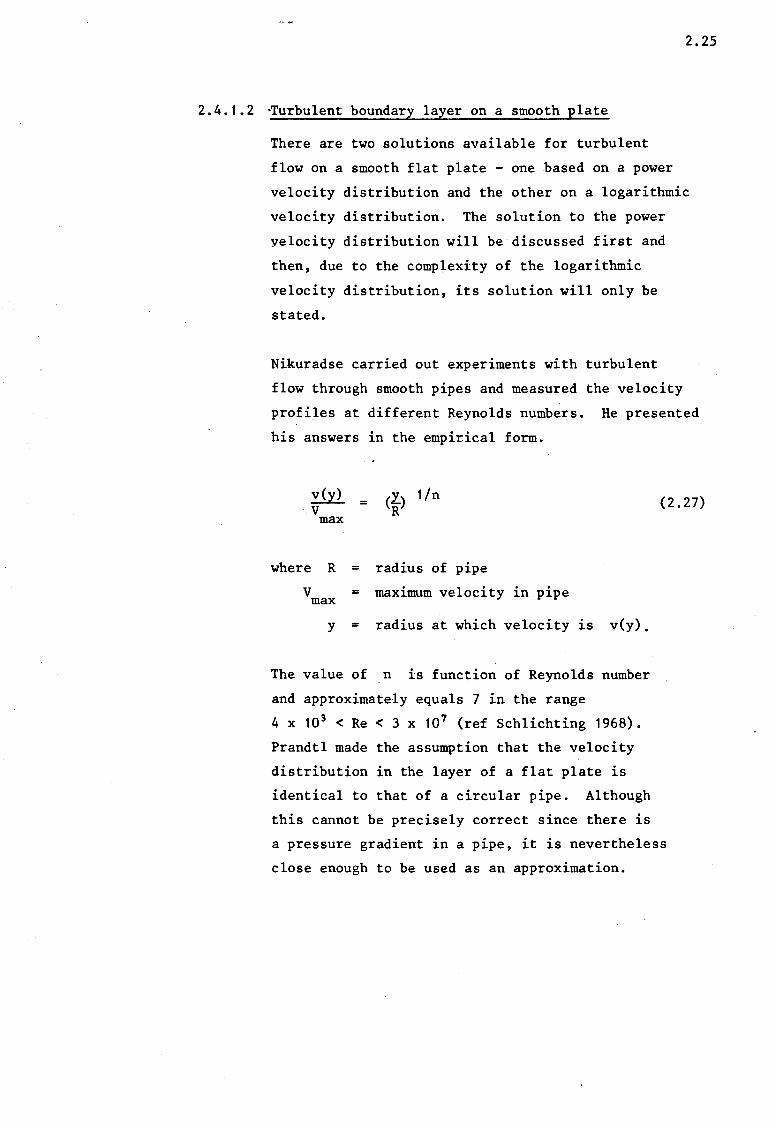
2.4.1.2 -Turbulent boundary layer on a smooth plate
There are two solutions available for turbulent
flow on a smooth flat plate - one based on a power
velocity distribution and the other on a logarithmic
velocity distribution. The solution to the power
yelocity distribution will be discussed first and
then, due to the complexity of the logarithmic
velocity distribution, its solution will only be
stated.
Nikuradse carried out experiments with turbulent
flow through smooth pipes and measured the velocity
profiles at different Reynolds numbers. He presented
his answers in the empirical form.
v(y) -v- =
max (1-) 1/n R
where R = radius of pipe
V = maximum velocity in pipe max
y = radius at which velocity is v(y).
The value of n is function of Reynolds number
and approximately equals 7 in the .range
4 x 10 3 <Re< 3 x 10⁷ (ref Schlichting 1968).
Prandtl made the assumption that the velocity
distribution in the layer of a flat plate is
identical to that of a circular pipe. Although
this cannot be precisely correct since there is
(2.27)
a pressure gradient in a pipe, it is nevertheless
close enough to be used as an approximation.
Univers
ity of
Cap
e Tow
n
Therefore, we have the following approximate
velocity distribution in the turbulent boundary
layer of a flat plate (see Figure 2.7 page 2.22).
2.26
v v max
= (2.28)
substituting this into Equation 2.23 and solving
=
=
=
0 p v2 f
0 <v -) < 1
max
7 = n p v2 0.
v v max
) dy
(2.29)
To obtain information about the wall shear stress
T , we use the relationship established by Blasius 0
for Reynolds number in pipe flow
T (Re)-1/4 0 0,08 (2.30) =
i P v2
where Re Reynolds number of pipe VD = = -
\)
V = Mean velocity
D = Diameter of pipe.
Univers
ity of
Cap
e Tow
n
We need Equation 2.30 in terms of radius and
maximum velocity. Using the relationship
(ref Kilner notes 1983)
v max
v = 1,24
and D . = 2R
v Re = max . 2R
1,24 v
for
=
Rewriting Equation 2.30
Re < 3 x 10 7
1,6129 V R max v
'r 0
I p v2 2 max = (
Vmax R -1 /4 0 ,0462 " )
And now using the analogy between the flat plate
2.27
(2.31)
and circular pipe we take V as the free stream max velocity V and o as the thickness of the boundary
layer. Therefore, we can now write .Equation 2.31 as
applied to a flat plate
'r = 0
Differentiating Equation 2.29 with respect to x
we get
T 0
dF = dx
7 v2 do = n P dx
(2.32)
(2.33)
Univers
ity of
Cap
e Tow
n
Equating Equations 2.32 and 2.33
1 do 0,0231
<vo)1/4 v
= 72.dx
x f 0,2374 dx =
0
0,2374 x =
Raising to 4/5
0,3165 x 415
0 f (Vo) 1/4 do v
0
(~) 1/5 (0,8365)0
O = 0,37 :x; (Re )- 1/ 5 :x;
Therefore, in a turbulent boundary layer o increases with ·X to the 0,8 power compared
to the laminar boundary layer case where O
increases with x to 0,5 power.
Substituting Equation 2.34 into Equation 2.29
0,036 p v2 :x; (Re )-l/5 x
giving the skin friction acting on one side of
the plate. Thus the skin friction coefficient
is given by
= ! P v2 = 0,072 (Re )-l/5 x
Re < 10 7 x
2.28
(2.34)
(2.35)
(2.36)
Univers
ity of
Cap
e Tow
n
A better correlation with experimental results
has been found by changing the numerical constant
to 0,074, therefore
2.29
= 0,074 (Re )-1/ 5 x Re < 107
x (2. 37)
Equation 2.36 is known as the Prandtl-von Karman
line and is illustrated in Figure 2.8 page 2.24.
The solution to the logarithmic velocity distribu
tion has been found to fit an empirical equation
of the form
= 0,455
(log Re ) 2 , 58 x
(2.38)
This equation is valid for the whole range of
Reynolds numbers up to Re· = 109 • See Figure 2.8 x
page 2.24.
2.4.1.3 Laminar and turbulent flow on a smooth flat plate.
Unless the flow is disturbed before reaching the
plate the flow after the leading edge will .be
laminar and if the critical value of Reynolds
number is reached further down the plate the
transition from laminar to turbulent flow will
take place. In order to allow for the initial
length of laminar flow we need to make the following
correction (ref Schlichting 1968).
= 0,455
(log Re ) 2 , 58 x
A Re x
(2.39)
Univers
ity of
Cap
e Tow
n
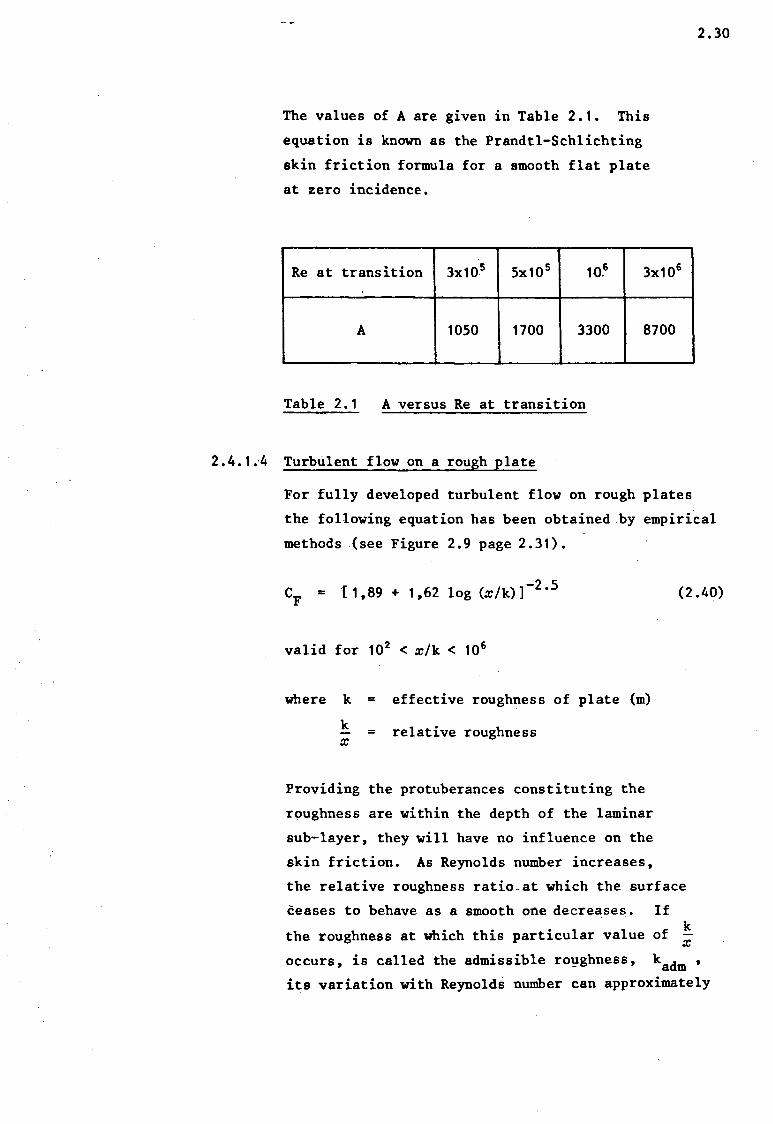
The values of A are given in Table 2.1. This
equation is known as the Prandtl-Schlichting
skin friction formula for a smooth flat plate
at zero incidence.
Re at transition 3x10⁵ 5x10 5 10.6 3x10⁶
A 1050 1700 3300 8700
Table 2.1 A versus Re at transition
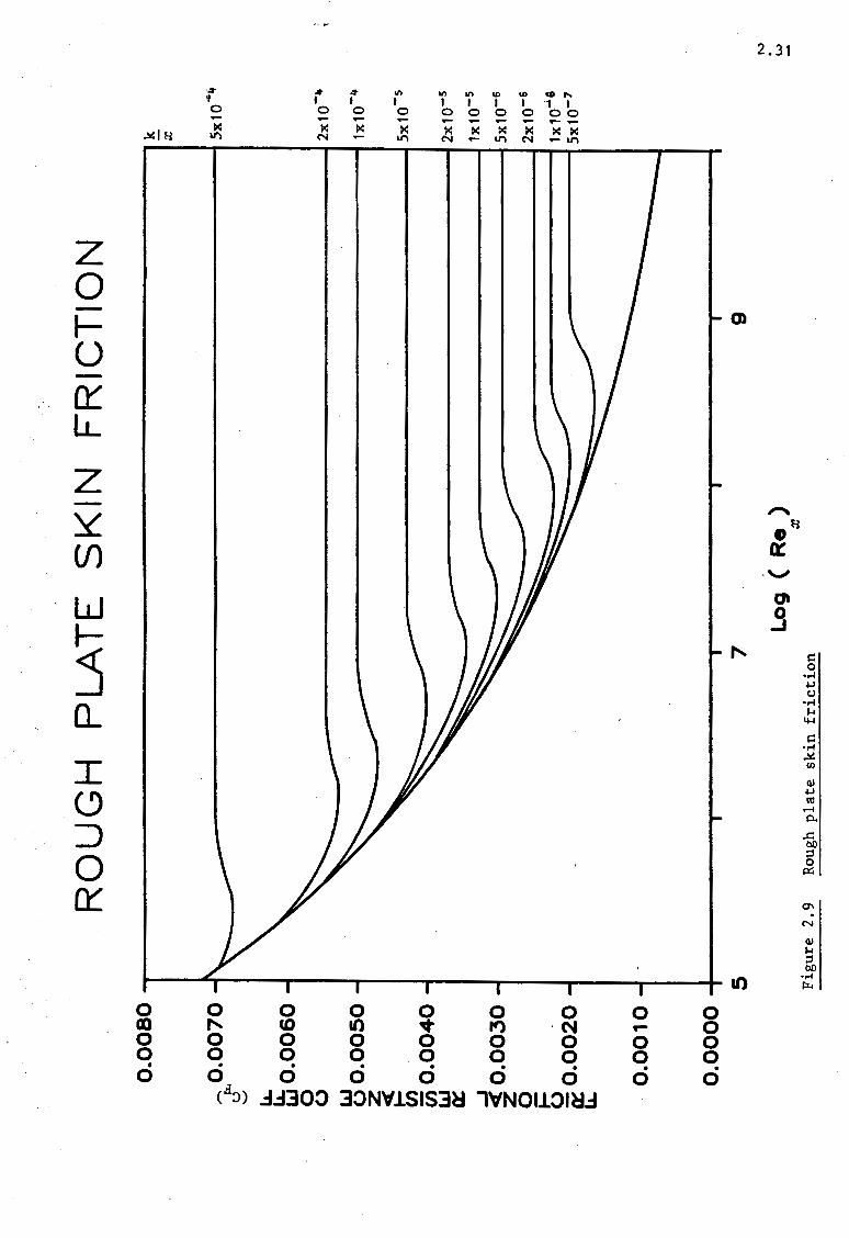
2.4.1 .. 4 Turbulent flow on a rough plate
2.30
For fully developed turbulent flow on rough plates
the following equation has been obtained.by empirical
methods (see Figure 2.9 page 2.31).
CF = {1,89 + 1,62 log (x/k)]-2•5
valid for 102 < x/k < 106
where k = effective roughness of plate (m)
k x
= relative roughness
Providing the protuberances constituting the
roughness are within the depth of the laminar
sub-layer, they will have no influence on the
skin friction. As Reynolds number increases,
(2.40)
the relative roughness ratio.at which the surface
ceases to behave as a smooth one decreases. If
the roughness at which this particular value of ~ occurs, is called the admissible ro~ghness, kadm ,
its variation with Reynolds number can approximately
Univers
ity of
Cap
e Tow
n
RO
UG
H
PL
AT
E
SK
IN
FR
ICT
ION
0
.00
80
k
-0
.00
70
~
'-"
LL.
LL.
LU 0
.00
60
0 0 LU
o
o.o
oso
z ~
(/) iii 0
.00
40
LU
0::
: _, ~ 0
.00
30
0 g
. ii:
0.0
02
0
LL. 0
.00
10
x Sx10
'""it
====
====
=----
--J 2x10-.. 1x
10-a
.
--~~~~~~~~~~~~~~~~~~~~__J5x10-s
== --=
==
==
==
=1
2x
10
-s
____
,,,,-
1x
10
-•
---::
sx1
0-•
_,,,,--
__ I 2x1
0-6
. 1x
10'"
"'
5x
10
-7
0.0000-t----------------------------------------------,,.----------~
5 7
9
Lo
g
( R
e )
x
Fig
ure
2
.9
Rou
gh
pla
te s
kin
fri
cti
on
N . w ....
Univers
ity of
Cap
e Tow
n 2.4.2
2.32
be given by the following formula (ref Todd 1966}
v k d am
" = 100
Therefore, the admissible roughness does not
depend on the length of the plate. A ship
travelling at a speed of 14 m/s will have an
admissible roughness of 0,007 unn, and while
travelling at 5 m/s an admissible roughness
of 0,02 unn. Clearly it is impossible to
obtain a hydraulically smooth ship hull and,
therefore, a correction due to hull roughness
will always have to be made when predicting
ship skin friction.
Skin friction acting on a ship
(2. 41)
The nature of the skin friction acting on a ship is similar
to that of a flat plate - the only difference being the
curvature of the hull which leads to radial pressure gradients
and velocities around the hull which are slightly greater than
the ship's speed through the water. If the velocity distri
bution within the boundary layer is known then it is possible
to exactly calculate the skin friction acting on the ship.
To determine the velocity distribution around a single hull
involves a substantial amount of work and time and is, there
fore, not a practical method of determining the skin friction
of a large number of hull forms. In order to provide quick
numerical values for skin friction, various skin friction
formulations have been developed.
The first of these formulations was developed by Froude after
his famous plank experiments in 1872.as was discussed in
Section 2.3.4. The form of Froude's equation.is as follows
= (2.42)

Univers
ity of
Cap
e Tow
n
SK
IN
FR
lCT
ION
F
OR
MU
LA
TIO
NS
0
.00
9-,-
--------,-
-----------,-
--------.-
---------r-----------
0.0
08
-J:>:.I C
,)
..._, I::
0.0
07
~
I I Pr
an
dtl
-vo
n K
arm
an
~ ~~
A.T
.T.C
. 0
\S
~
I.T
.T.C
. w
0
.00
6
0 z ~
0.0
05
(/
)
(/) w
0::
0.0
04
_. <
( z 0 0
.00
3
~ fE 0
.00
2
I I
I ··· .. -
~
0.0
01
O.O
OO
-+--
----
----
+--
----
----
t---
----
----
1--
----
----
-+--
----
----
-1
5 7
9
Log
( R
ex)
Fig
ure
2.1
0
Ski
n fr
icti
on
fo
rmu
lati
on
s
-------------
N . w
w
Univers
ity of
Cap
e Tow
n
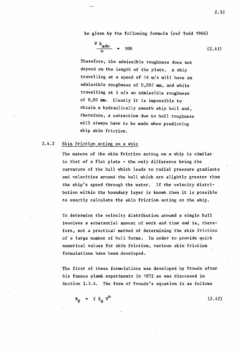
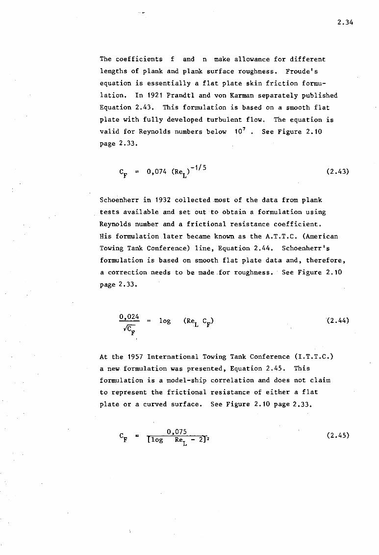
The coefficients f and n make allowance for different
lengths of plank and plank surface roughness. Froude's
equation is essentially a flat plate skin friction formu
lation. In 1921 Prandtl and von Karman separately published
Equation 2.43. This formulation is based on a smooth flat
plate with fully developed turbulent flow. The equation is
valid for Reynolds numbers below 107 • See Figure 2.10
page 2.33.
2.34
(2.43)
Schoenherr in 1932 collected most of the data from plank
tests available and set out to obtain a formulation using
Reynolds number and a frictional resistance coefficient.
His formulation later became known as the A.T.T.C. (American
Towing Tank Conference) line, Equation 2.44. Schoenherr's
formulation is based on smooth flat plate data and, therefore,
a correction needs to be made.for roughness. See Figure 2.10
page 2.33.
0,024 = log (2.44)
~
At the 1957 International Towing Tank Conference (I.T.T.C.)
a new formulation was presented, Equation 2.45. This
formulation is a model-ship correlation and does not claim
to represent the frictional resistance of either a flat
plate or a curved surface. See Figure 2.10 page 2.33.
= [log 0,075
Re - 2] 2 L
(2.45)
Univers
ity of
Cap
e Tow
n
I '
I I I
I I
The 1957 I.T.T.C. line has not been accepted by all
towing tanks and many still use frictional formulations
that are based on their own data collected during tests.
Therefore, there is, as yet, no completely standard
formulation for skin friction prediction.
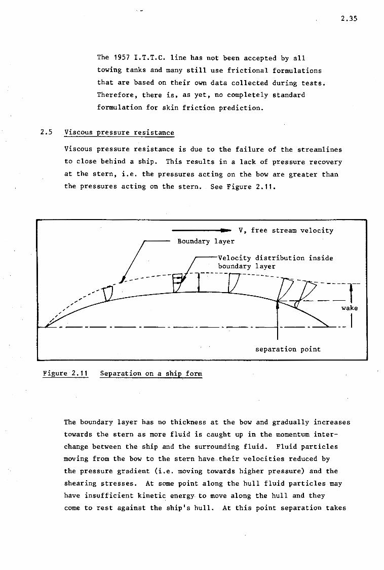
2.5 Viscous pressure resistance
2.35
Viscous pressure resistance is due to the failure of the streamlines
to close behind a ship. This results in a lack of pressure recovery
at the stern, i.e. the pressures acting on the bow are greater than
the pressures acting on the stern. See Figure 2.11.
V, free stream velocity
Boundary layer
r---velocity distribution inside boundary layer
---- ----- - - -
--- ---- ---- ----
separation point
Figure 2. 11 Separation on a ship form
The boundary layer has no thickness at the bow and gradually increases
towards the stern as more fluid is caught up in the momentum inter
change between the ship and the surrounding fluid. Fluid particles
moving from the bow to the stern have their velocities reduced by
the pressure gradient (i.e. moving towards higher pressure) and the
shearing stresses. At some point along the hull fluid particles may
have insufficient kinetic energy to move along the hull and they
come to rest against the ship's hull. At this point separation takes
Univers
ity of
Cap
e Tow
n
place, particles following are subsequently diverted away from
the hull causing vortices in the boundary layer and wake. Thus
from the separation point the flow lines leave the hull and distort
the pressure distribution in this zone, thus causing the failure
of the pressures at the stern to match the pressures at the bow.
The above phenomenon would not take place in an ideal fluid and
would also not arise on a flat plate. Therefore, viscous pressure
resistance is dependent on the viscosity of the fluid and the ship
form, increasing as viscosity increases and as the hull form becomes
more bluff.
2.6 Wave-making resistance
Wave-making resistance forms one of the most important components
of a ship's resistance even though it only becomes dominant at high
speeds. The viscous resistance of a conventional ship's hull cannot
be reduced significantly by changes to the hull shape. However, the
wave-making resistance can be reduced appreciably by modifications
to the hull ·shape. This has led to development of the bulbous bow
and wave-less forms (ref Inui 1962). Therefore, the importance of
wave-making resistance is that a knowledge of the relationship
between hull geometry and wave-making resistance can lead to the
development of optimum shaped hulls.
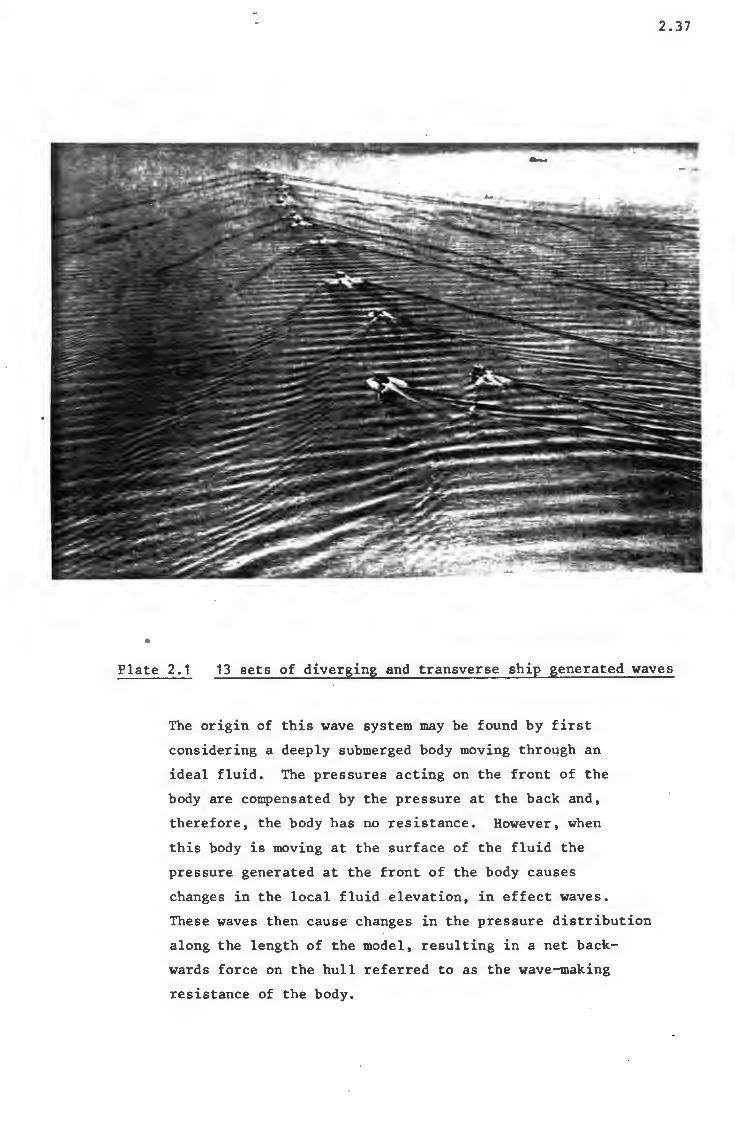
2.6.1 The nature of.wave-making resistance
A ship advancing with steady speed through calm sea disturbs
the surface in a regular wave pattern which moves with the
ship. The wave pattern consists of two systems of diverging
and transverse waves which are well illustrated in Plate 2.1
(ref Saunders 1972).
2.36
Univers
ity of
Cap
e Tow
n
2.37
•
Plate 2.1 13 sets of diverging and transverse ship generated waves
The origin of this wave system may be found by first
considering a deeply submerged body moving through an
ideal fluid. The pressures acting on the front of the
body are compensated by the pressure at the back and,
therefore, the body has no resistance. However, when
this body is moving at the surface of the fluid the
pressure generated at the front of the body causes
changes in the local fluid elevation, in effect waves.
These waves then cause changes in the pressure distribution
along the length of the model, resulting in a net back
wards force on the hull referred to as the wave-making
resistance of the body.
Univers
ity of
Cap
e Tow
n
The ship generated wave system and, therefore, also
the wave-making resistance is a function of:
a, Speed with which the ship moves through the water
b. The depth of the water
c. Geometric proportions of the ship
d. Size of the ship.
The wave.systemwill remain constant for a ship moving
at constant speed and through water of uniform depth.
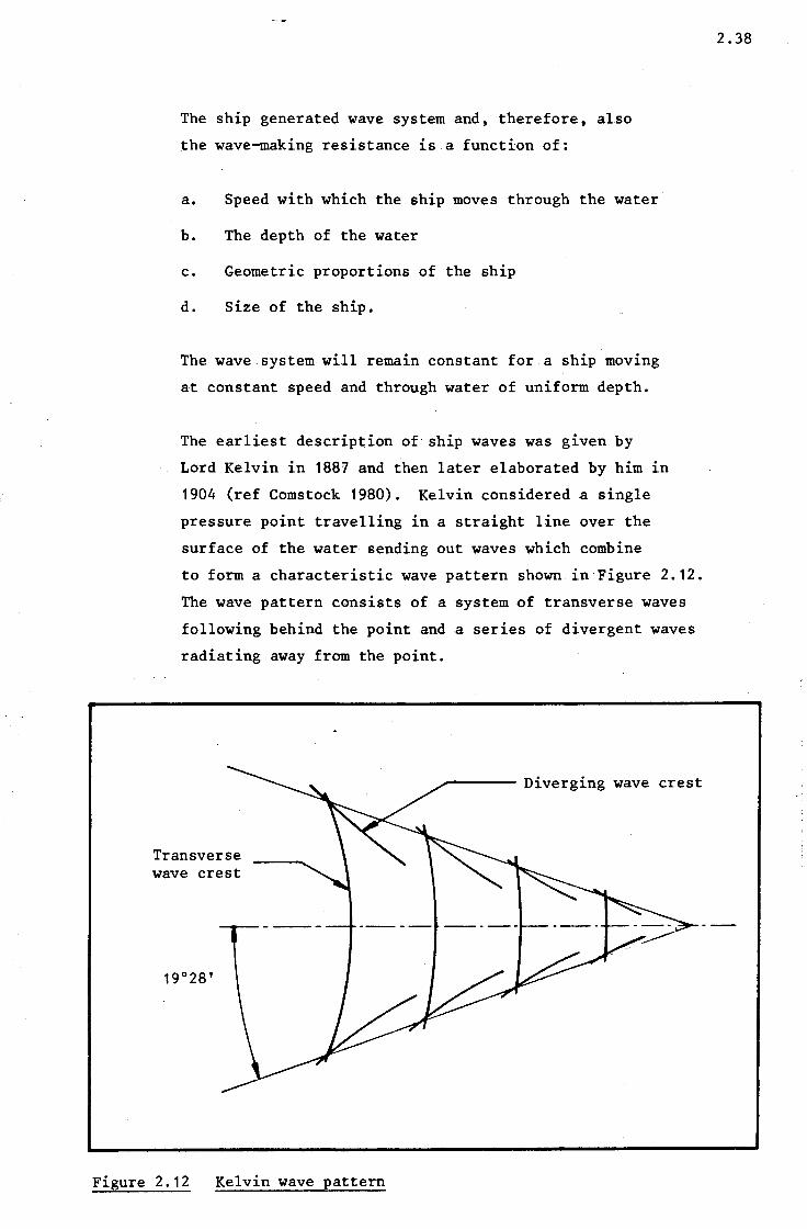
The earliest description of ship waves was given by
Lord Kelvin in 1887 and then later elaborated by him in
1904 (ref Comstock 1980). Kelvin considered a single
pressure point travelling in a straight line over the
surf ace of the water sending out waves which combine
to form a characteristic wave pattern shown in Figure 2.12.
The wave pattern consists of a system of transverse waves
following behind the point and a series of divergent waves
radiating away from the point •
Transverse wave crest
19°28'
Figure 2.12 Kelvin wave pattern
.-~~~- Diverging wave crest
2.38
Univers
ity of
Cap
e Tow
n
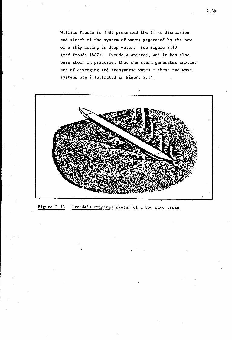
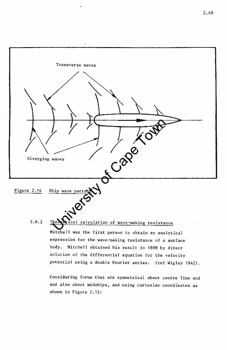
William Froude in 1887 presented the first discussion
and sketch of the system of waves .generated by the bow
of a ship moving in deep water. See Figure 2.13
(ref Froude 1887). Froude suspected, and.it has also
been shown in practice, that the stern generates another
set of diverging and transverse waves - these two wave
systems are illustrated in Figure 2.14.
Figure 2.13 Froude's original sketch.of a bow wave train
2.39
Univers
ity of
Cap
e Tow
n
Transverse waves
\ y
Diverging waves /
Figure 2.14
2.6.2
Ship wave pattern
Theoretical calculation of wave-making resistance
Mitchell was the first person to obtain an analytical
expression for the wave-making resistance of a surface
body. Mitchell obtained his result in 1898 by direct
solution of the differential equation for the velocity
potential using a double Fourier series. (ref Wigley 1942).
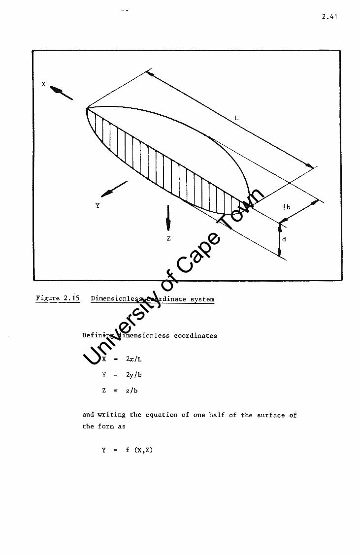
Considering forms that are symmetrical about centre line and
and also about midships, and using cartesian coordinates as
shown in Figure 2.15:
2.40
Univers
ity of
Cap
e Tow
n
Figure 2.15
y
' z
Dimensionless coordinate system
Defining dimensionless coordinates
X 2x/L
y = 2y/b
Z z/b
and writing the equation of one half of the surface of
the form as
Y f (X,Z)
2.41

Univers
ity of
Cap
e Tow
n
2.6.3
The wave resistance of the form specified in the above
equation is given by
=
where
J =
~ JTI/2(I2 + J2) sec3 9d9
TIIJ2
bd T
0
1 +1 J J (~)e-dgZsec2 S/V2 sin(LgXsec8/ZV2 )dXdZ 0 -1
2.42
(2.46)
I = bd T
1 +1 J J (~)e-dgZsec2 S/V2
cos(LgXsec8/ZV2 )dXdZ 0 -1
This solution is based on the following assumptions:
a. The wave height .1s small compared ¥ith wave-length
b. The water velocities due to wave motion are small
compared with the speed of advance
c. The effects of turbulence and viscosity can be
neglected
d. Trim and sinkage of the form do not alter its wave
making characteristics appreciably.
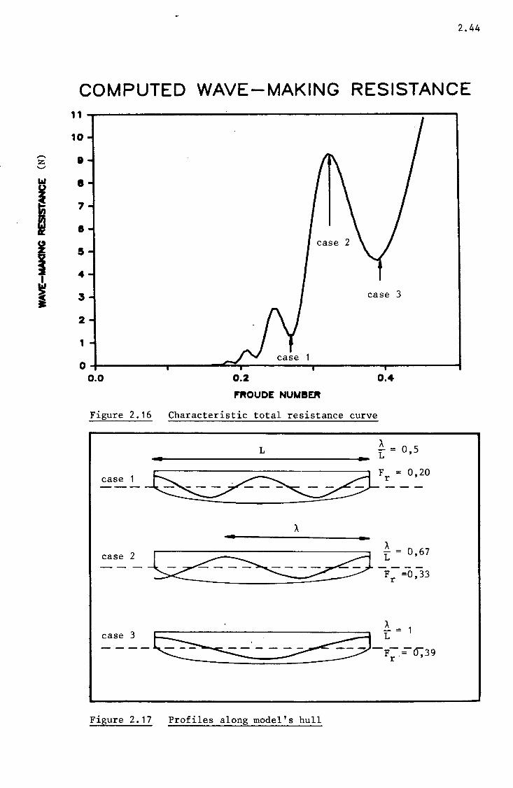
"Humps and hollows" in resistance curves
Figure 2.16 shows the theoretical wave-making resistance
computed from Equation 2.46. The form of the model is one
used in the author's experiments which are discussed in
Chapter 5. The curve displays the characteristic "humps
and hollows" of a total resistance curve, although the
amplitude of the deviations are exaggerated, since no
allowance 1s made for viscosity in the calculation. The
Univers
ity of
Cap
e Tow
n
source of these undulations in the resistance curve may
be explained by considering the wave length of the
transverse waves in relation to the length of the ship.
The speed of the transverse waves can reasonably be
expected to have the same speed as the ship has moving
through the water. The wave length and speed of a deep
water wave is given by (ref Sorenson 1973)
c 0
= .8!. 2TI = speed of deep water wave
2.43
).. 0
~ T2 2TI = wave length of deep water wave
Combining these two equations and recognising that
).. = 0
2nv2
g
c 0
The transverse wave length is plotted along the length
of the ship's hull in Figure 2.17 for a number of Froude
numbers. From this diagram it is clear that the humps
in the resistance curve occur when the surface levels at
the stern are low, while hollows occur when the surface
level is relatively high at the stern. Noting that the
pressures at the stern are significantly affected by the
local water height, it is apparent that the undulations
of the resistance curve are a function of the positioning
v
(2.47)
of the transverse waves along the ship's length as generated
by the bow.
Univers
ity of
Cap
e Tow
n
2.44
COMPUTED WAVE-MAKING RESISTANCE
case 3
0.2 0.4
FROUOE NUMBEft
Figure 2.16 Characteristic total resistance curve
L A. - = 0 5 L '
. A . cas.'.'_ 2_ I ~ ------4 _L ~ ~,67 ~~~Fr=0,33
. A -=1
c•i: _:_ -~· ~ - ;;:i•S;L~; ;-0:39
Figure 2.17 Profiles along model's hull
Univers
ity of
Cap
e Tow
n
CHAPTER 3
EXPERIMENTAL MEASUREMENT TECHNIQUES
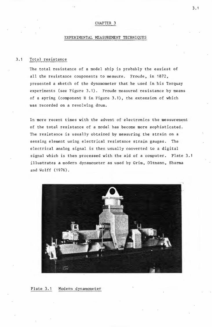
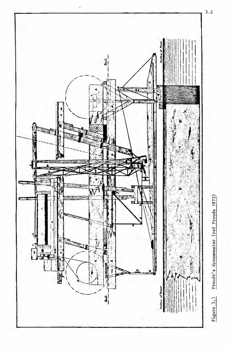
3.1 Total resistance
The total resistance of a model ship is probably the easiest of
all the resistance components to measure. Froude, in 1872,
presented a sketch of the dynamometer that he used in his Torquay
experiments (see Figure 3.1). Froude measured resistance by means
of a spring (component Hin Figure 3.1), the extension of which
was recorded on a revolving drum.
In more recent times with the advent of electronics the measurem~nt
of the total resistance of a model has become more sophisticated.
The resistance is usually obtained by measuring the strain on a
sensing element using electrical resistance strain gauges. The
electrical analog signal is then usually converted to a digital
signal which is then processed with the aid of a computer. Plate 3.1
illustrates a modern dynamometer as used by Grim, Oltmann, Sharma
and Wolff (1976).
Plate 3.1 Modern dynamometer
3. 1
Univers
ity of
Cap
e Tow
n
-
---
•
3.2
Cl) -Q)
"'Cl =' 0 ,...
µ..
Univers
ity of
Cap
e Tow
n
3.3
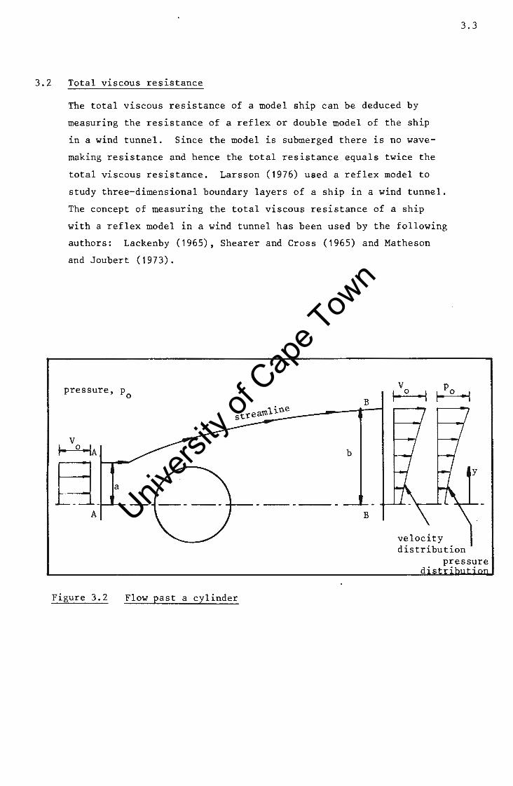
3.2 Total viscous resistance
The total viscous resistance of a model ship can be deduced by
measuring the resistance of a reflex or double model of the ship
in a wind tunnel. Since the model is submerged there is no wave
making resistance and hence the total resistance equals twice the
total viscous resistance. Larsson (1976) used a reflex model to
study three-dimensional boundary layers of a ship in a wind tunnel.
The concept of measuring the total viscous resistance of a ship
with a reflex model in a wind tunnel has been used by the following
authors: Lackenby (1965), Shearer and Cross (1965) and Matheson
and Joubert (1973).
pressure, p0
b
a
- -------A
B
B
Vo po I- ·I ~ •I
velocity distribution
y
p:essi.;re
Figure 3.2 Flow past a cylinder
Univers
ity of
Cap
e Tow
n
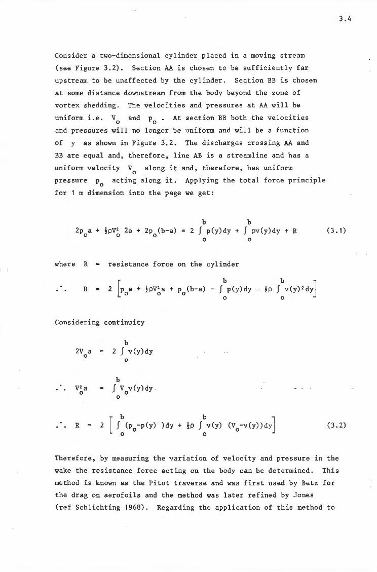
Consider a two-dimensional cylinder placed in a moving stream
(see Figure 3.2). Section AA is chosen to be sufficiently far
upstream to be unaffected by the cylinder. Section BB is chosen
at some distance downstream from the body beyond the zone of
vortex shedding. The velocities and pressures at AA will be
uniform i.e. v and Po . At section BB both the velocities 0
and pressures will no longer be uniform and will be a function
of y as shown in Figure 3.2. The discharges crossing AA and
BB are equal and, therefore, line AB is a streamline and has a
uniform velocity V along it and, therefore, has uniform 0
pressure p0
acting along it. Applying the total force principle
for 1 m dimension into the page we get:
b b
3.4
2p a + !pV2 2a + 2p (b-a) = 2 J p(y)dy + J pv(y)dy + R 0 0 0
(3. 1) 0 0
where R = resistance force on the cylinder
R = 2 [p a+ !pV2a + p (b-a) - Jbp(y)dy - !P Jbv(y)2dyJ 0 0 0
0 0
Considering continuity
b 2V a 2 J v(y)dy
0 0
b V2a J v v(y)dy
0 0 0
R [ b b J 2 J (p
0-p(y) )dy + !P J v(y) (V
0-v(y))dy
0 0
(3. 2)
Therefore, by measuring the variation of velocity and pressure in the
wake the resistance force acting on the body can be determined. This
method is known as the Pitot traverse and was first used by Betz for
the drag on aerofoils and the method was later refined by Jones
(ref Schlichting 1968). Regarding the application of this method to
Univers
ity of
Cap
e Tow
n
three-dimensional bodies Lackenby (1965) has shown that the
results agree closely with those obtained by a dynamometer.
Tulin (1951) has also suggested that the method can be applied
to the determination of the total viscous resistance of a
surface body and thus represents a method of separating wave
making and viscous resistance. The Pitot traverse method has
been used by Lackenby (1965), Shearer (1965) and Townsin (1971).
3.3 Skin friction
When a fluid flows past a ship's hull it exerts normal and shear
stresses on the hull surface. The measurement of the normal stress
or pressure is relatively simple (discussed in Section 3.4), however,
the measurement of the shear stress or the local skin friction is
a more complicated task. If the velocity distribution at a point
along the hull is known, the local shear stress may be calculated
using Equation 3.3. By integrating the local shear stress over a
small area dA the local skin friction can be calculated
3.5
(3 .3)
This method entails making numerous measurements to obtain the
velocity distribution close to the hull which gives the value of
the local shear stress at one point only. To obtain the variation
of the skin friction over the hull the above procedure has to be
repeated at other locations along the hull. Obviously this method
is time consuming and hence expensive. As a result simpler and
less time consuming methods have been developed to measure local
skin friction.
3.3.1 Direct measurements
The shear stress at the hull can be measured directly by
using a transducer. The transducer is usually calibrated
by direct force application. Since the transducers do not
reply on the behaviour of the boundary layer they are in
principle the most reliable method of measuring shear stress.
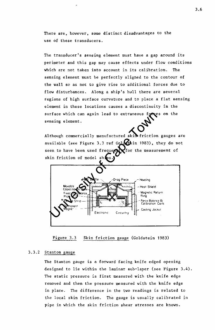
Univers
ity of
Cap
e Tow
n
There are, however, some distinct disadvantages to the
use of these transducers.
The transducer's sensing element must have a gap around its
perimeter and this gap may cause effects under flow conditions
which are not taken into account in its calibration. The
sensing element must be perfectly aligned to the contour of
the wall so as not to give rise to additional forces due to
flow disturbances. Along a ship's hull there are several
regions of high surf ace curvature and to place a flat sensing
element in these locations causes a discontinuity in the
surface which can again lead to extraneous forces on the
sensing element.
Although commercially manufactured skin friction gauges are
available (see Figure 3.3 ref Goldstein 1983), they do not
seem to have been used frequently for the measurement of
skin friction of model ships.
Heat Baffle -·,
' Movab le Capac itonce Plate ~:::::;:=:::;;;-
F 1xed Copoc1tonce
Plate -::=tttl~~~~ Flexure St ri p
Permanent Mogne! -
Housing
- Heat Shield
-- Magnet 1c Return R ing
Force Balance 8 Calibration Coils
- Cooling J ocktt
Figure 3.3 Skin friction gauge (Goldstein 1983)
3.3.2 Stanton gauge
The Stanton gauge is a forward facing knife edged opening
designed to lie within the laminar sub-layer (see Figure 3.4).
The static pressure is first measured with the knife edge
removed and then the pressure measured with the knife edge
in place. The difference in the two readings is related to
the local skin friction. The gauge is usually calibrated in
pipe in which the skin friction shear stresses are known.
3.6

Univers
ity of
Cap
e Tow
n
3.7
The pressure differences are generally very small and, therefore,
it is necessary to use a micromanometer with an accuracy of
_:: 0,01 nrrn (ref Goldstein 1983). Great care needs to be taken
to keep the distance of the knife edge above the hole constant.
Problems arise in water in that the suspended solids, such as
are usually present, may clog the knife edge (ref Steele and
Pearce 1967).
The Stanton gauge has largely been superseded by the Preston
tube as a method of measuring skin friction on model ships.
h,--Local Sur face Asymmetric Razor Blade Flow Direction
Razor Blode
lb I I
I ~--'~~~~__. _J_
Figure 3.4 Stanton gauge (Goldstein 1983)
3 . 3.3 Preston tube
The Preston tube is a forward-facing total head tube placed
adjacent to the surface of a body where the skin friction
measurement is to be made (see Figure 3.5). The Preston
tube is larger than the Stanton gauge and does not remain
within the laminar sub-layer. The static pressure is first
measured and then compared to the pressure measured with the
total head tube in place. The pressure difference is then
related to the local skin friction. The Preston tube is
usually calibrated in a pipe and was first done so by Preston
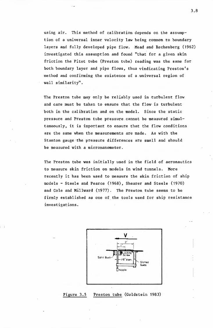
Univers
ity of
Cap
e Tow
n
3.8
using air. This method of calibration depends on the assump
tion of a universal inner velocity law being common to boundary
layers and fully developed pipe flow. Mead and Rechenberg (1962)
investigated this assumption and found "that for a given skin
friction the Pitot tube (Preston tube) reading was the same for
both boundary layer and pipe £.lows, thus vindicating Preston's
method and confirming the existence of a universal region of
wall similarity".
The Preston tube may only be reliably used in turbulent flow
and care must be taken to ensure that the flow is turbulent
both in the calibration and on the model. Since the static
pressure and Preston tube pressure cannot be measured simul
taneously, it is important to ensure that the flow conditions
are the same when the measurements are made. As with the
Stanton gauge -the pressure differences are small and should
be measured with a micromanometer.
The Preston tube was initially used in the field of aeronautics
to measure skin friction on models in wind tunnels. More
recently it has been used to measure the skin friction of ship
models - Steele and Pearce (1968), Shearer and Steele (1970)
and Cole and Millward (1977). The Preston tube seems to be
firmly established as one of the tools used for ship resistance
investigations.
Figure 3.5
Spl it Bush
Slot ted Guide
Preston tube (Goldstein 1983)
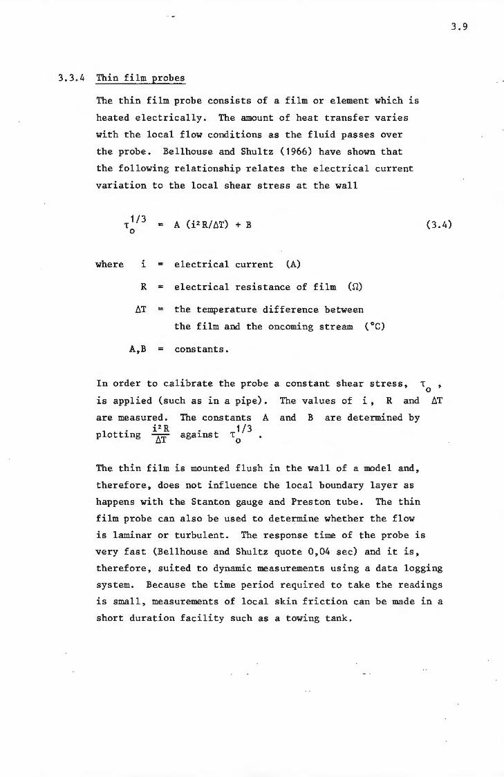
Univers
ity of
Cap
e Tow
n
3.3.4 Thin film probes
The thin film probe consists of a film or element which is
heated electrically. The amount of heat transfer varies
with the local flow conditions as the fluid passes over
the probe. Bellhouse and Shultz (1966) have shown that
the following relationship relates the electrical current
variation to the local shear stress at the wall
where
1/3 T A (i2R/6T) + B
0
i electrical current (A)
R electrical resistance of film (~)
6T = the temperature difference between
the film and the oncoming stream (°C)
A,B = constants.
In order to calibrate the probe a constant shear stress, T
(3. 4)
0
is applied (such as in a pipe). The values of i , R and 6T
are measured. The constants A and B are determined by . i 2 R . 1 /3
plotting 6T against T0
The thin film is mounted flush in the wall of a model and,
therefore, does not influence the local boundary layer as
happens with the Stanton gauge and Preston tube. The thin
film probe can also be used to determine whether the flow
is laminar or turbulent. The response time of the probe is
very fast (Bellhouse and Shultz quote 0,04 sec) and it is,
therefore, suited to dynamic measurements using a data logging
system. Because the time period required to take the readings
is small, measurements of local skin friction can be made in a
short duration facility such as a towing tank.
3.9
Univers
ity of
Cap
e Tow
n
Most of the work done using thin film probes has been done
in air e.g. Davies and Kimber (1976). However, Pope and
Bellhouse (1971) used thin film probes to measure local skin
friction on a model ship. They found good agreement with the
results obtained from Preston tubes. The major problem
encountered was that small bubbles of air present in the water
collected on the model. These air bubbles had to be removed
prior to each test to ensure that the bubbles did not cause
any inaccuracies as they would have greatly influenced the
heat transfer rate.
Although the thin film probes are relatively expensive to
manufacture, they have great potential for the measurement of
local skin friction. They offer a fast and simple measurement
because the instrument output is electrical.
3.4 Total pressure resistance
Consider a small hole or tapping made in the side of a model and
connected to a manometer - the fluid level in the manometer will
equal the still water level when the model is stationery. If the
model is now moved through the fluid the water level will either
rise or drop relative to the still water level depending on the
location of the tapping on the hull. The pressure difference ~p
1s related to pressure resistance experienced by the model and will
be positive at the bow and usually negative at the stern.
If the model's hull is covered with an array of pressure tappings
each having a defined area, dA and the pressure differences are
recorded when the model 1s moving through a fluid the total pressure
resistance can be found by the following equation
where
R p
= J ~p cos¢ dA
8w
wetted surface area
¢ = angle between the normal to the surface dA and
direction of motion.
(3.5)
3. 10

Univers
ity of
Cap
e Tow
n
Therefore, the evaluation of the total pressure resistance is
relatively simple. However, great care must be taken to ensure
that the tappings are drilled normal to the surf ace and that there
are no burrs around the holes as this would affect the measured
pressure. Generally the pressures are measured using a manometer
which has the advantage of accuracy but has a slow response and
can, therefore, only be used in situations where steady state can
be achieved for a reasonable length of time. Electronic pressure
transducers may be used instead of manometers if steady state can
only be achieved for a short duration as their response time is
much faster.
Some of the authors that have conducted pressure tapping experiments
on model ships are Froude (1874), Lackenby (1965), Shearer and Cross
(1965), and Matheson and Joubert (1973).
3.5 Wave-making resistance
A ship moving through still water generates a set of gravity waves
and in doing so, therefore, expends energy which is associated with
wave-making resistance ;for a known ship movement. If the change in
amount of energy stored in the ship wave pattern could be measured,
the wave-making resistance of the ship could be determined. There
fore, the problem has two components: firstly, to determine the
wave pattern and secondly, having obtained the wave pattern, to
calculate the wave-making resistance.
A conmen way to obtain the ship wave pattern is to place wave-height
recorders at fixed points and then measure the wave pattern as the
model passes. A novel method of determining the wave pattern has
been developed at the University of Cape Town by Paterson (1986).
A model is towed across a basin filled with an opaque fluid and a
pair of stereo photographs taken. These photographs are later
analysed in a stereo comparator and a contour map of the wave pattern
produced. The method is interesting because the possibility exists
of taking stereo photographs of full scale ships in protected waters.
The methods of analysis vary but generally they consist of either
taking a transverse cut or a longitudinal cut of the wave pattern,
ref Wehausen (1973).
3. 11
Univers
ity of
Cap
e Tow
n
CHAPTER 4
EXPERIMENTAL OBJECTIVES
4.1 Objectives
The purpose of the experimental investigation was to measure
directly as many of the resistance components as possible, or
failing this, to be able to deduce the resistance components
not directly measured. From the start it was felt that the
direct measurement of skin friction and wave-making resistance
were beyond the scope of the investigation and, therefore, these
two components would have to be obtained by difference. This lead
to two sets of experiments - one aimed at deducing the wave-making
resistance and the other at inferring skin friction. For practical
reasons these two sets of experiments were conducted at different
scales, in different facilitie~ in the geometric ratio of 2,7 to 1.
To determine the skin friction component of total resistance a model
had pressure tappings located on it and thus the total pressure
resistance measured. By measuring the total resistance and sub
tracting the pressure component the skin friction could be deduced.
In order to measure the pressure distribution a fairly long steady
state time period is required and to achieve this a glass flume
in the U C T hydraulics laboratory was used. Water is supplied to
the glass flume from a constant head tank and, therefore, the same
flow conditions can be maintained indefinitely.
The wave-making resistance was to be found by measuring the total
resistance of a model placed at the water surface and then measuring
4. 1
the total resistance of the corresponding reflex model deeply submerged.
Half of the total resistance of the deeply submerged body would equal
the total viscous resistance of the surface body and, therefore, if
subtracted from the total resistance of the surface body the difference
would be the wave-making resistance. Since the length of steady state
is not too critical for the reflex experiment, use was made of the
towing channel facility in U C T Civil Engineering laboratory.
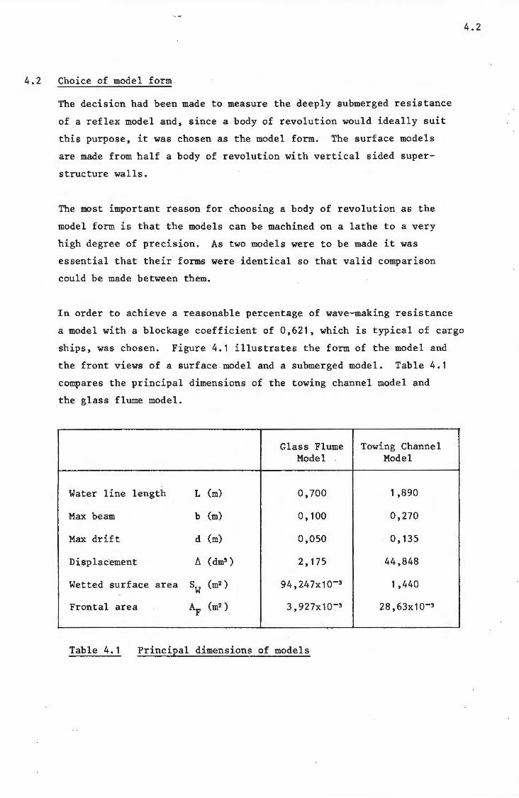
Univers
ity of
Cap
e Tow
n
4.2 Choice of model form
The decision had been made to measure the deeply submerged resistance
of a reflex model and, since a body of revolution would ideally suit
this purpose, it was chosen as the model form. The surface models
are made from half a body of revolution with vertical sided super
structure walls.
The most important reason for choosing a body of revolution as the
model form is that the models can be machined on a lathe to a very
high degree of precision. As two models were to be made it was
essential that their forms were identical so that valid comparison
could be made between them.
In order to achieve a reasonable percentage of wave-making resistance
a model with a blockage coefficient of 0,621, which is typical of cargo
ships, was chosen. Figure 4.1 illustrates the form of the model and
the front views of a surface model and a submerged model. Table 4.1
compares the principal dimensions of the towing channel model and
the glass flume model.
Glass Flume Towing Channel Model Model
Water line length L (m) 0,700 1 ,890
Max beam b (m) 0' 100 0,270
Max drift d (m) 0,050 0' 135
Displac·ement /;.. (dm3 ) 2,175 44,848
Wetted surface area SW (m2) 94, 247x10-3 1 ,440
Frontal area AF (m2) 3, 927x 10-3 28 ,63x10-3
Table 4. 1 Principal d~mensions of models
4.2
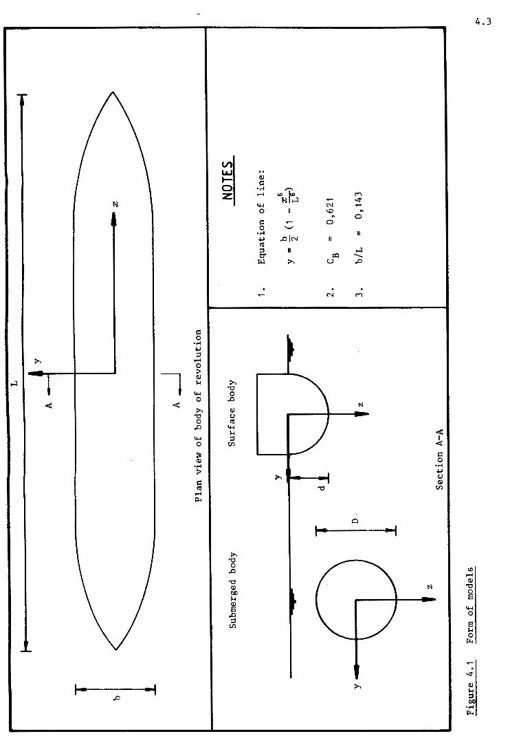
Univers
ity of
Cap
e Tow
n
L
I y
A
b
A _
J P
lan
vie
w o
f bo
dy o
f re
vo
luti
on
Sub
mer
ged
body
S
urf
ace
body
y
d
D
y .-
......
. -..
..--
---.
z
z S
ecti
on
A-A
Fig
ure
4
. 1
Form
o
f m
odel
s
1.
2.
3.
x
NOTE
S
Eq
uat
ion
of
lin
e:
b :;r
;6
y =
-( 1
-T
T)
2 L
CB
=
0,62
1
b/L
=
0
' 143
~
VJ
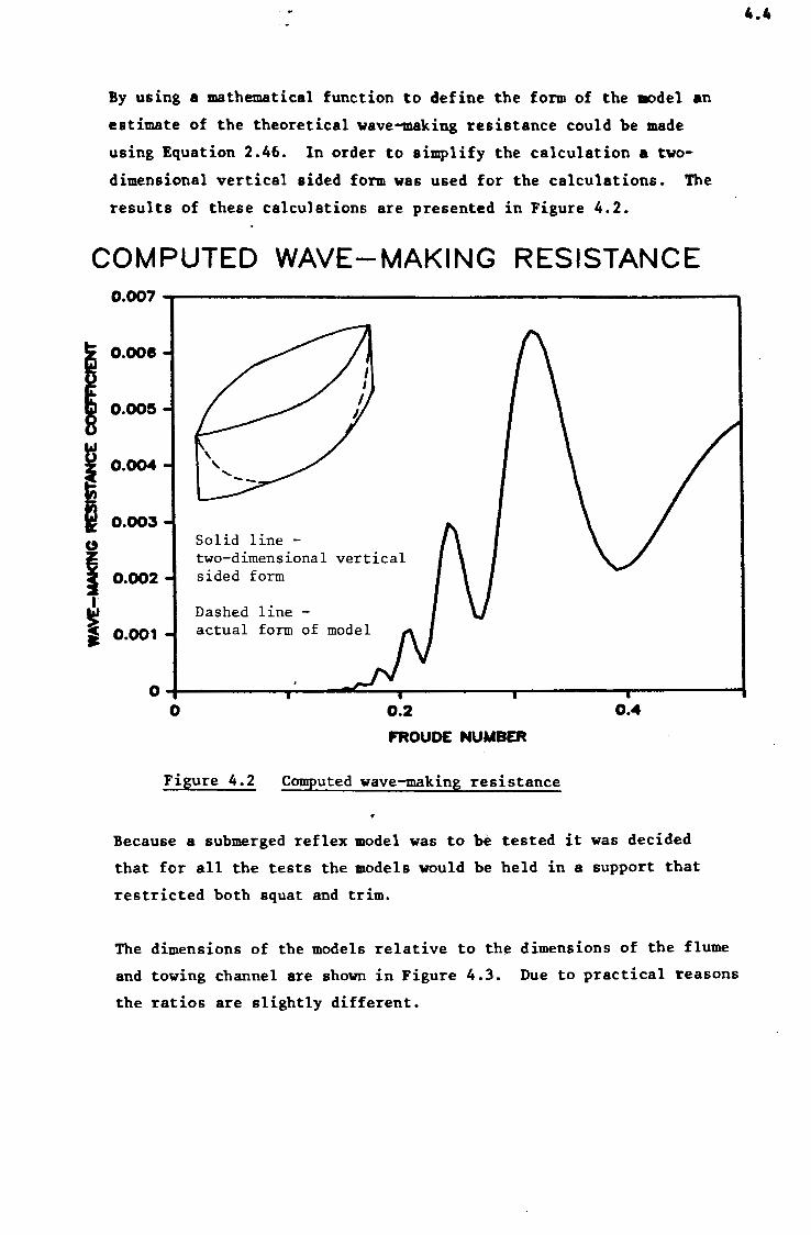
Univers
ity of
Cap
e Tow
n
By using a mathematical function to define the form of the model an
estimate of the theoretical wave-making resistance could be made
using Equation 2.46. In order to simplify the calculation a two
dimensional vertical sided form was used for the calculations. The
results of these calculations are presented in Figure 4.2.
COMPUTED WAVE-MAKING RESISTANCE
o.ooe
0.00~
~ 0.004
I O.OOJ
I i 0.002
Solid line -two-dimensional vertical sided form
I
~ • 0.001
0
Dashed line -actual form of
0.2
f'ROUOE NUMBER
Figure 4.2 Computed wave-making resistance
0.4
Because a submerged reflex model was to be tested it was decided
that for all the tests the models would be held in a support that
restricted both squat and trim.
The dimensions of the models relative to the dimensions of the flume
and towing channel are shown in Figure 4.3. Due to practical reasons
the ratios are slightly different.
4.4
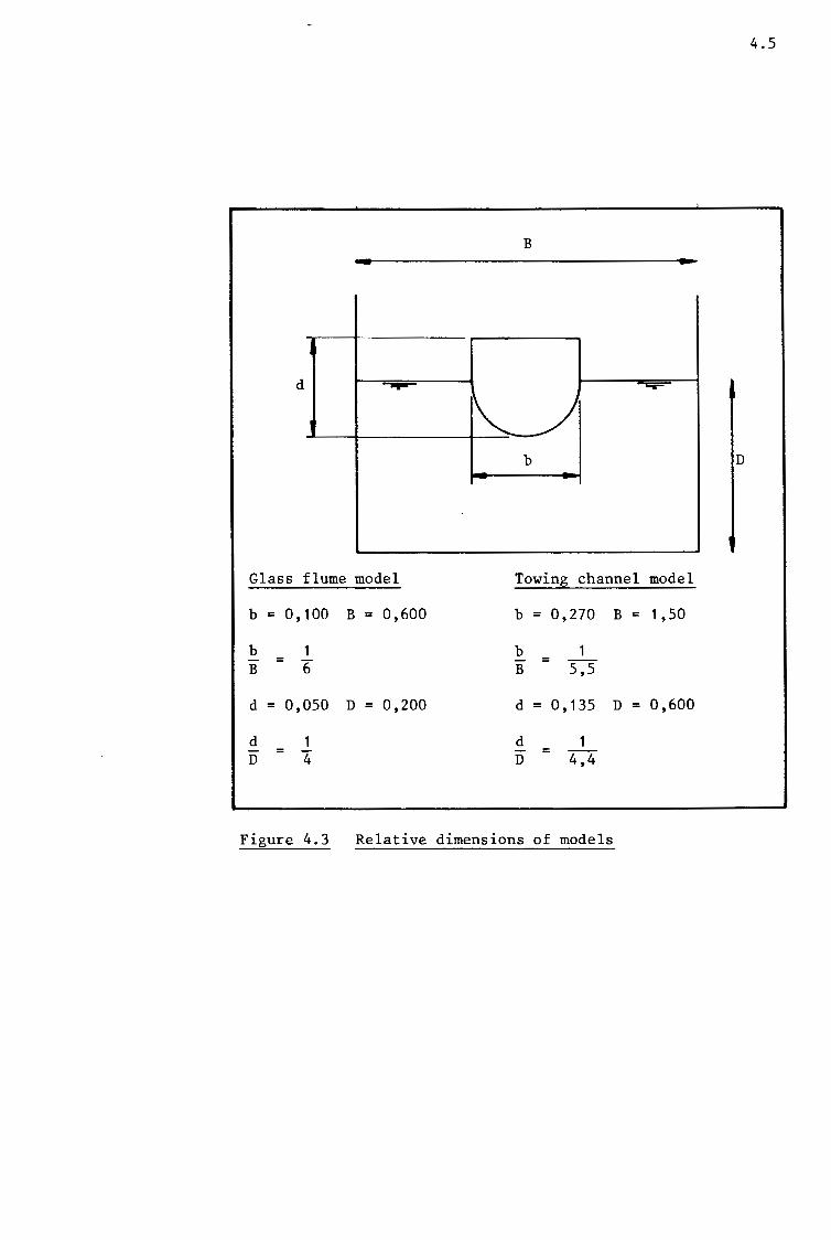
Univers
ity of
Cap
e Tow
n
4.5
B
d -,,:pr- ~
~ b D
Glass flume model Towing channel model
b = 0, 100 B = 0,600 b = 0,270 B = 1 ,50
b 1 b = 6 = 5,5 B B
d 0,050 D = 0,200 d = 0, 135 D 0,600
d 1 d = 4 = 4,4 D D
Figure 4.3 Relative dimensions of models
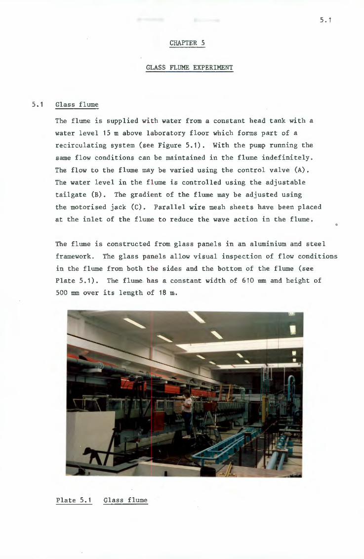
Univers
ity of
Cap
e Tow
n
CHAPTER 5
GLASS FLUME EXPERIMENT
5. 1 Glass flume
The flume is supplied wi t h water from a constant head tank with a
water level 15 m above l aboratory floor which forms part of a
recirculating system (see Figure 5.1). With the pump running the
same flow conditions can be maintained in the flume indefinitely.
The flow to the flume may be varied using the control valve (A).
The water level in the f l ume is controlled using the adjustable
tailgate (B). The gradient of the flume may be adjusted using
5 . 1
the motorised jack (C). Parallel wire mesh sheets have been placed
at the inlet of the flume to reduce the wave action in the flume. •
The flume is constructed from glass panels in an aluminium and steel
framework. The glass panels allow visual inspection of flow conditions
in the flume from both t he sides and the bottom of the flume (see
Plate 5.1). The flume has a constant width of 610 mm and height of
500 mm over its length of 18 m.
Plate 5.1 Glass flume
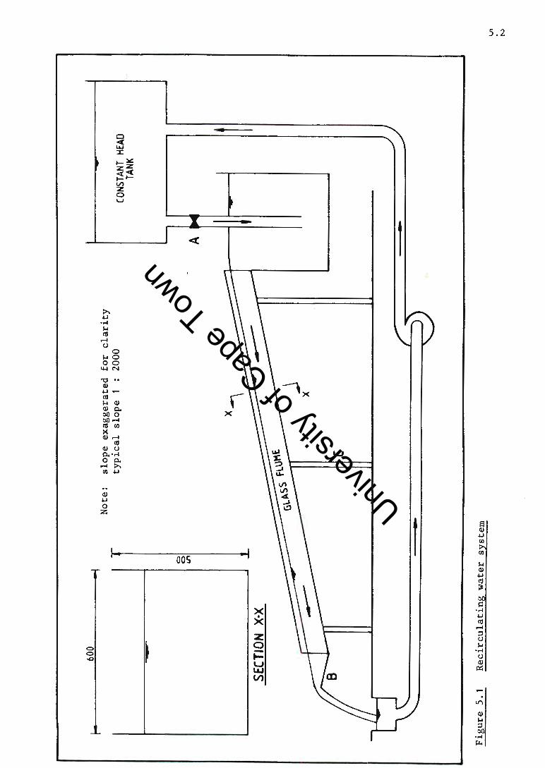
Univers
ity of
Cap
e Tow
n
I·
600
_1
---
SECT
ION
X-X
C>
C
> "'
Fig
ure
5
.1
Recir
cu
lati
ng
wat
er
syst
em N
ote
: sl
op
e ex
agg
erat
ed fo
r cla
rity
ty
pic
al
slo
pe
1 :
2000
x
(
A
j
CONS
TANT
HE
AD
TANK
1
Vl . N
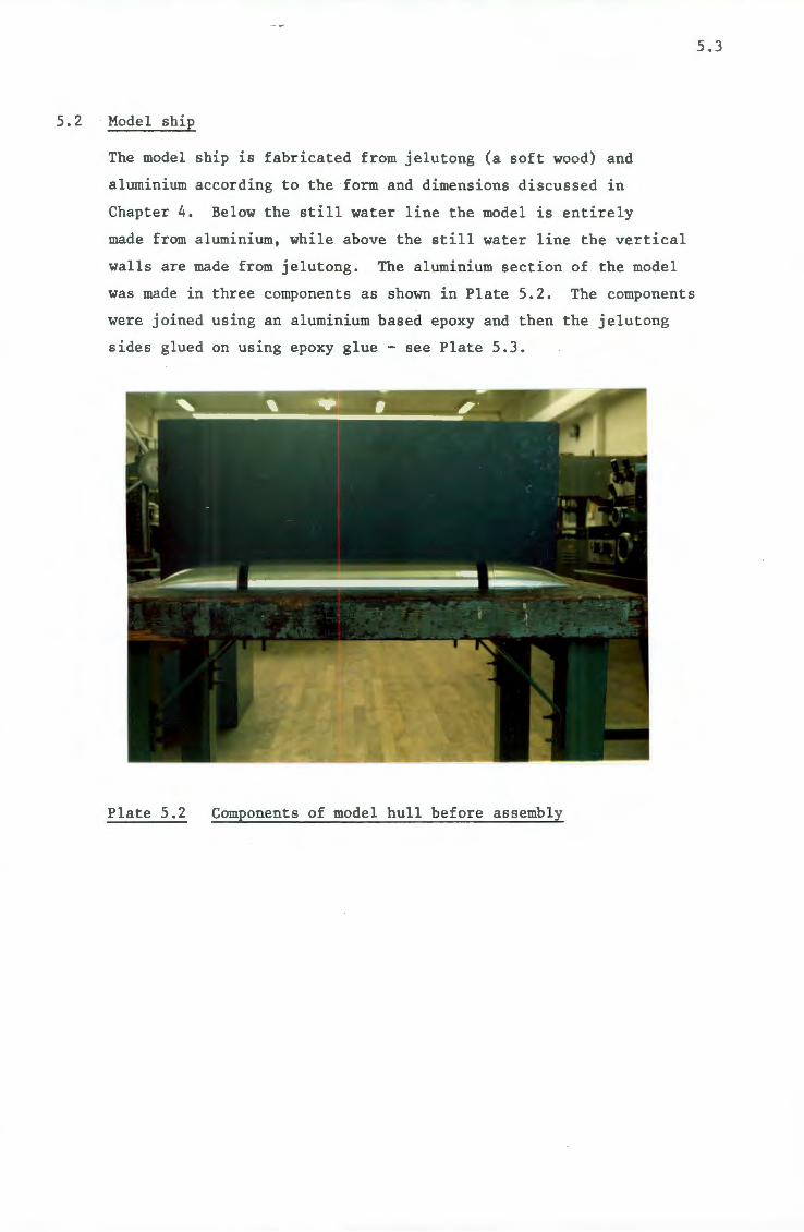
Univers
ity of
Cap
e Tow
n
5.2 Model ship
The model ship is fabricated from jelutong (a soft wood) and
aluminium according to the form and dimensions discussed in
Chapter 4. Below the stil l water line the model is entirely
made from aluminium, while above the still water line the vertical
walls are made from jelutong. The aluminium section of the model
was made in three component s as shown in Plate 5.2. The components
were joined using an aluminium based epoxy and then the jelutong
sides glued on using epoxy glue - see Plate 5.3.
Plate 5.2 Components of model hull before assembly
5.3
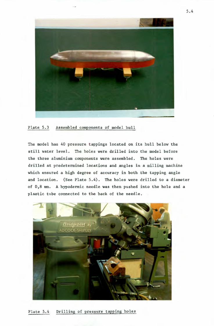
Univers
ity of
Cap
e Tow
n Plate 5.3 Assembled components of model hull
The model has 40 pressure t appings located on its hull below the
still water level. The holes were drilled into the model before
the three aluminium components were assembled. The holes were
drilled at predetermined locations and angles in a milling machine
which ensured a high degree of accuracy in both the tapping angle
5.4
and location. (See Plate 5.4). The holes were drilled to a diameter
of 0,8 mm. A hypodermic needle was then pushed into the hole and a
plastic tube connected to t he back of the needle.
Plate 5.4 Drilling of pressure tapping holes
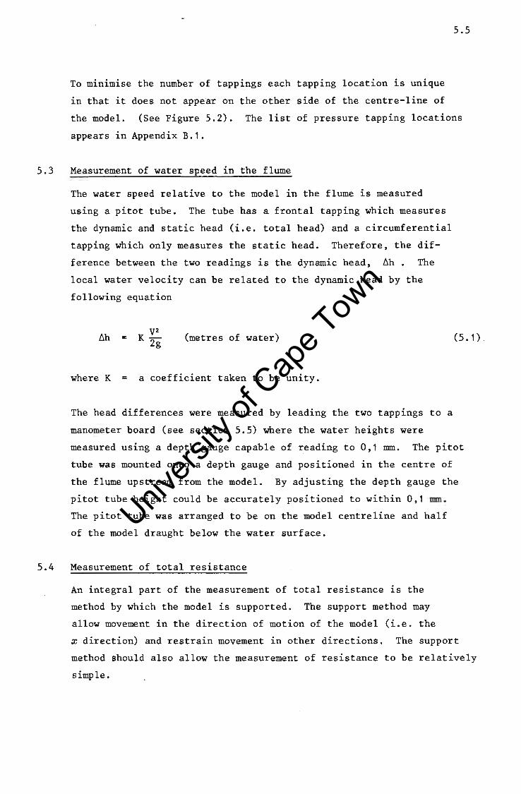
Univers
ity of
Cap
e Tow
n
5.5
To minimise the number of tappings each tapping location is unique
in that it does not appe~r on the other side of the centre-line of
the model. (See Figure 5.2). The list of pressure tapping locations
appears in Appendix B.1.
5.3 Measurement of water speed in the flume
The water speed relative to the .model in the flume is measured
using a pitot tube. The tube has a frontal tapping which measures
the dynamic and static head (i.e. total head) and a circumferential
tapping which only measures the static head. Therefore, the dif
ference between the two. readings is the dynamic head, ~h • The
local water velocity can be related to the dynamic head by the
following equation
~h
where K
v2 = K-2g (metres of water)
a coefficient taken to be unity.
(5. 1) '
The head differences were measured by leading the two tappings to a
manometer board (see section 5.5) where the water heights were
measured using a depth gauge capable of reading to 0,1 mm. The pitot
tube was mounted onto a depth gauge and positioned in the centre of
the flume upstream from the model. By adjusting the depth gauge the
pitot tube height could be accurately positioned to within 0,1 mm.
The pitot tube was arranged to be on the model centreline and half
of the model draught below the water surface.
5.4 Measurement of total resistance
An integral part of the measurement of toral resistance is the
method by which the model is supported . The support method may
allow movement in the direction of motion of the model (i.e. the
x direction) and restrain movement in other directions. The support
method should also allow the measurement of resistance to be relatively
simple.
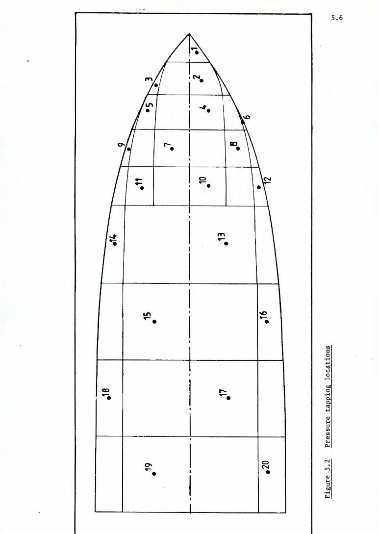
Univers
ity of
Cap
e Tow
n
.1e
I I
.14
I - -
.19
I I
15
.11
• I
I I
.1
-~1
-1-.
~ I -
~;-r-
.2
I .1
1 I
I .1
3 .a
I
I ...
b .2
0 I
I • 1
6
Fig
ure
5
.2
Pre
ssu
re
tap
pin
g
locati
on
s V
l . 0\
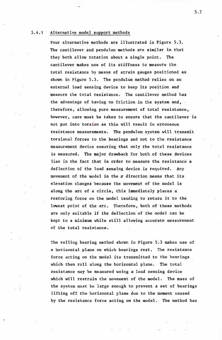
Univers
ity of
Cap
e Tow
n
5. 4. 1 Alternative model support methods
Four alternative methods are illustrated in Figure 5.3.
The cantilever and pendulum methods are similar in that
they both allow rotation about a single point. The
cantilever makes use of its stiffness to measure the
total resistance by means of strain gauges positioned as
shown in Figure 5.3. The pendulum method relies on an
external load sens ing device to keep its position and
measure the total resistance. The cantilever method has
5.7
the advantage of having no friction in the system and,
therefore, allowing pure measurement of total resistance,
however, care mus t be taken to ensure that the cantilever is
not put into tors i on as this will result in erroneous
resistance measurements. The pendulum system will transmit
torsional forces t o the bearings and not to the resistance
measurement device ensuring .that only the total resistance
is measured. The major drawback for both of these devices
lies in the fact t hat in order to measure the resistance a
deflection of the load sensing device is required. Any
movement of the model in the x direction means that its
elevation changes because the movement of the model is
along the arc of a circle, this immediately places a
restoring force on the model tending to return it to the
lowest point of t he arc. Therefore, both of these methods
are only suitable if the deflection of the model can be
kept to a minimum while still allowing accurate measurement
of the total resistance.
The rolling bearing method shown in Figure 5.3 makes use of
a horizontal plane on which bearings rest. The resistance
force acting on the model its transmitted to the bearings
which then roll along the horizontal plane. The total
resistance may be measured using a load sensing device
which will restra in the movement of the model. The mass of
the system must be large enough to prevent a set of bearings
lifting off the horizontal plane due to the moment caused
by the resistance force acting on the model. The method has

Univers
ity of
Cap
e Tow
n
Can
tile
ver
met
hod
str
ain
gau
ges
Ro
llin
g
bea
rin
g m
etho
d
beari
ng
Fig
ure
5
.3
Alt
ern
ati
ve
sup
po
rt m
etho
ds
ho
rizo
nta
l su
rface
Pen
dulu
m m
etho
d
beari
ng
Air
tr
ack
met
hod
air
tr
ack
tr
oll
ey
\JI
(X)
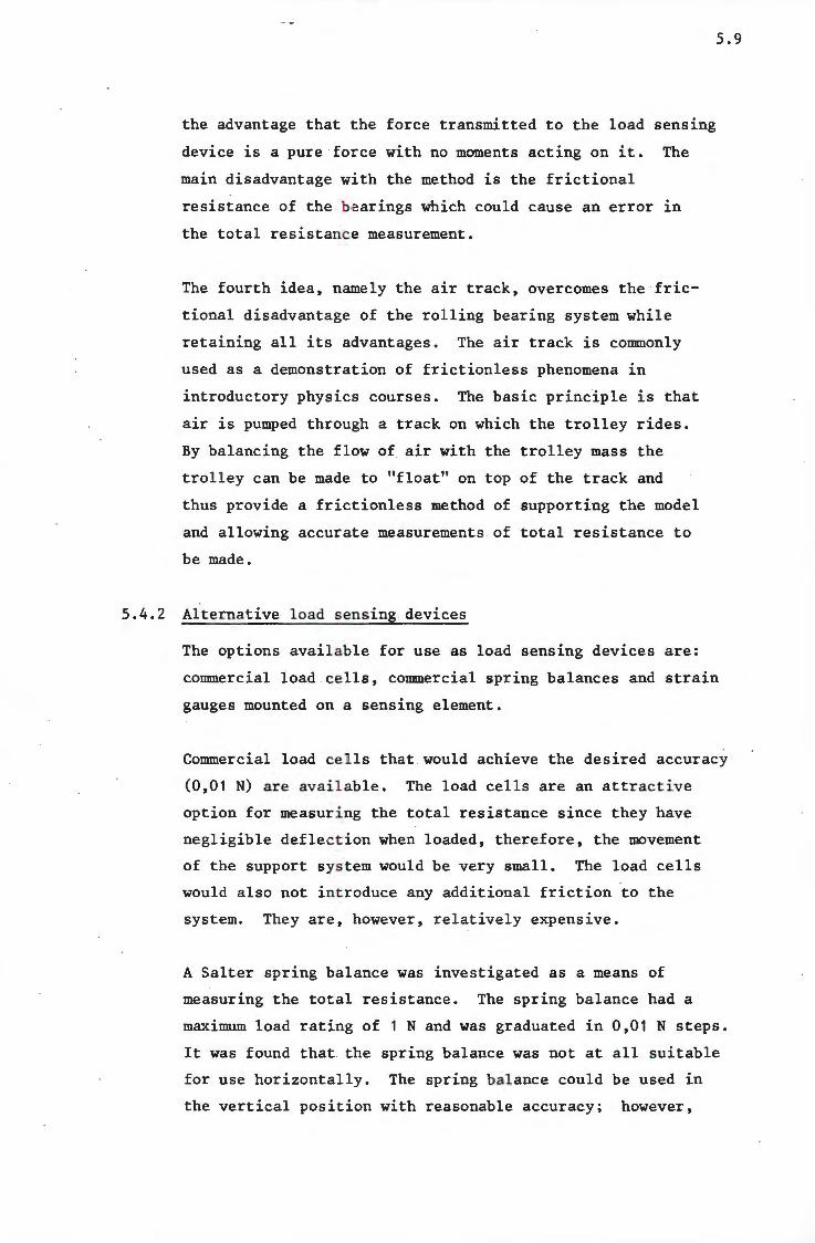
Univers
ity of
Cap
e Tow
n
the advantage that the force transmitted to the load sensing
device is a pure force with no moments acting on it. The
main disadvantage with the method is the frictional
resistance of the bearings which could cause an error in
the total resistance measurement.
The fourth idea, namely the air track, overcomes the fric
tional disadvantage of the rolling bearing system while
retaining all its advantages. The air track is commonly
used as a demonstration of frictionless phenomena in
introductory physics courses. The basic principle is that
air is pumped through a track on which the trolley rides.
By balancing the flow of air with the trolley mass the
trolley can be made to "float" on top of the track and
thus provide a frictionless method of supporting the model
and allowing accurate measurements . of total resistance to
be made.
5.4.2 Alternative load sensing devices
5.9
The options available for use as load sensing devices are:
commercial load cells, commercial spring balances and strain
gauges mounted on a sensing element.
Commercial load cells that would achieve the desired accuracy
(0,01 N) are avai l able. The load cells are an attractive
option for measur i ng the total resistance since they have
negligible deflect ion when loaded, therefore, the movement
of the support sys tem would be very small. The load cells
would also not introduce any additional friction to the
system. They are, however, relatively expensive.
A Salter spring balance was investigated as a means of
measuring the total resistance. The spring balance had a
maximum load rating of 1 N and was graduated in 0,01 N steps.
It was found that the spring balance was not at all suitable
for use horizontally. The spring balance could be used in
the vertical position with reasonable accuracy; however,
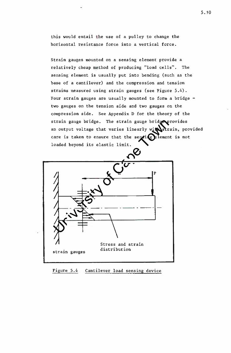
Univers
ity of
Cap
e Tow
n
this would entail t he use of a pulley to change the
horizontal resistance force into a vertical force.
Strain gauges mount ed on a sensing element provide a
relatively cheap method of producing "load cells". The
sensing element is usually put into bending (such as the
base of a cantilever) and the compression and tension
strains measured using strain gauges (see Figure 5.4).
Four strain gauges are usually mounted to form a bridge -
two gauges on the tension side and two gauges on the
compression side. See Appendix D for the theory of the
strain gauge bridge. The strain gauge bridge provides
5 .10
an output voltage that varies linearly with strain, provided
care is taken to ensure that the sensing element is not
loaded beyond its elastic limit.
I
strain gauges
Figure 5.4
L p
----------- -
Stress and strain distribution
Cantilever load sensing device
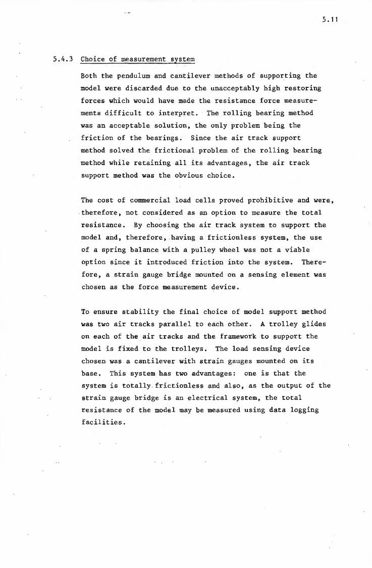
Univers
ity of
Cap
e Tow
n
5.4.3 Choice of measurement system
Both the pendulum and cantilever methods of supporting the
model were discarded due to the unacceptably high restoring
forces which would have made the resistance force measure
ments difficult to interpret. The rolling bearing method
was an acceptable solution, the only problem being the
friction of the bearings. Since the air track support
method solved the frictional problem of the rolling bearing
method while retaining all its advantages, the air track
support method was the obvious choice.
5. 11
The cost of connnercial load cells proved prohibitive and were,
therefore, not considered as an option to measure the total
resistance. By choosing the air track system to support the
model and, therefore, having a frictionless system, the use
of a spring balance with a pulley wheel was not a viable
option since it introduced friction into the system. There
fore, a strain gauge bridge mounted on a sensing element was
chosen as the force measurement device.
To ensure stability the final choice of model support method
was two air tracks parallel to each other. A trolley glides
on each of the air tracks and the framework to support the
model is fixed to the trolleys. The load sensing device
chosen was a cantilever with strain gauges mounted on its
base. This system has two advantages: one is that the
system is totally . frictionless and also, as the output of the
strain gauge bridge is an electrical system, the total
resistance of the model may be measured using data logging
facilities .
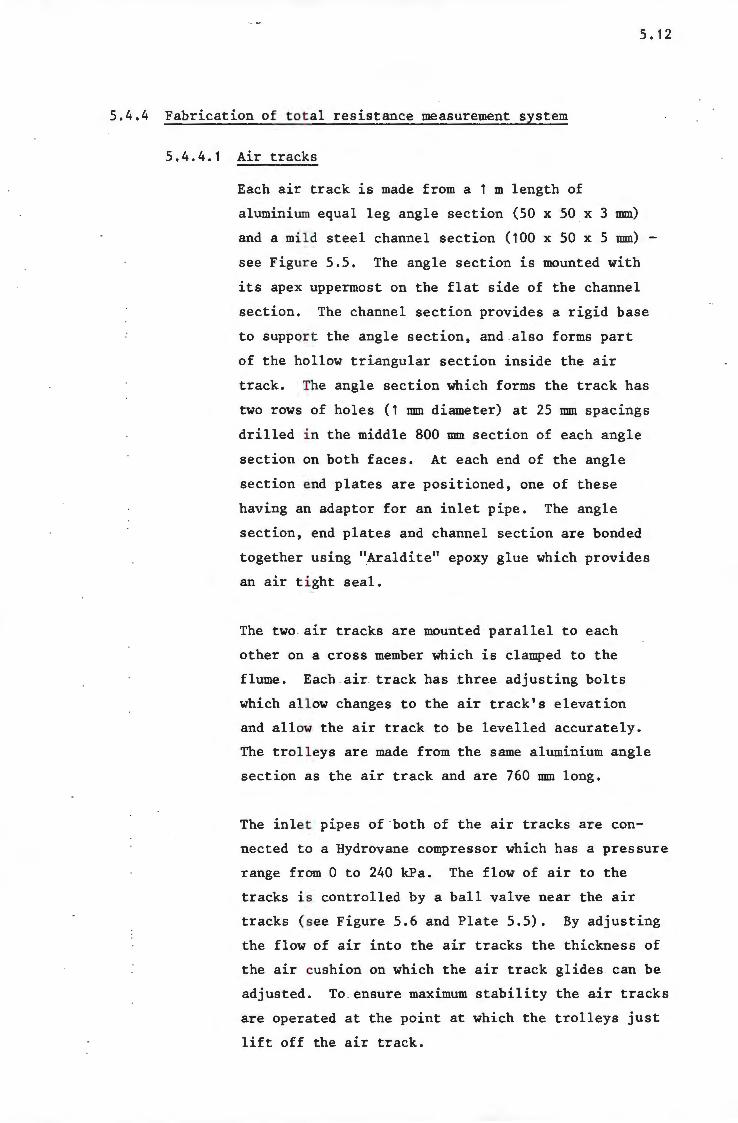
Univers
ity of
Cap
e Tow
n
5. 12
5.4.4 Fabrication of to t al resistance measurement system
5.4.4.1 Air tracks
Each air track is made from a 1 m length of
aluminium equal leg angle section (50 x 50 x 3 mm)
and a mi l d steel channel section (100 x 50 x 5 mm) -
see Figur e 5.5. The angle section is mounted with
its apex uppermost on the flat side of the channel
section. The channel section provides a rigid base
to suppor t the angle section, and also forms part
of the hollow triangular section inside the air
track. The angle section which forms the track has
two rows of holes (1 mm diameter) at 25 mm spacings
drilled i n the middle 800 mm section of each angle
section on both faces. At each end of the angle
section end plates are positioned, one of these
having an adaptor for an inlet pipe. The angle
section, end plates and channel section are bonded
together using ".Araldite" epoxy glue which provides
an air t i ght seal.
The two air tracks are mounted parallel to each
other on a cross member which is clamped to the
flume. Each .air track has three adjusting bolts
which al l ow changes to the air track's elevation
and allow the air track to be levelled accurately.
The trol l eys are made from the same aluminium angle
section as the air track and are 760 mm long.
The inle t pipes of both of the air tracks are con
nected to a Hydrovane compressor which has a pressure
range from 0 to 240 kPa. The flow of air to the
tracks i s controlled by a ball valve near the air
tracks ( see Figure 5.6 and Plate 5.5). By adjusting
the flow of air into the air tracks the thickness of
the air cushion on which the air track glides can be
adjusted . To ensure maximum stability the air tracks
are operated at the point at which the trolleys just
lift off the air track.
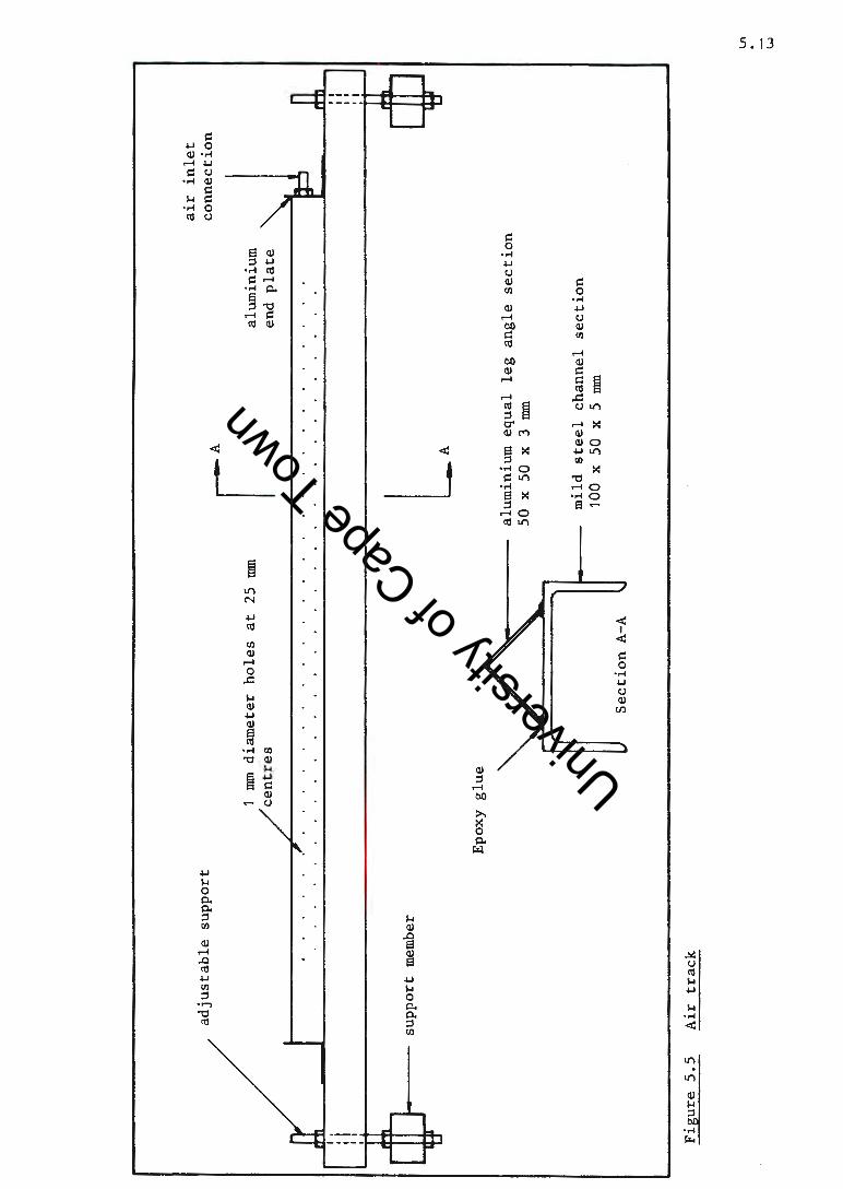
Univers
ity of
Cap
e Tow
n
ad
just
ab
le
sup
po
rt
sup
po
rt m
embe
r
Fig
ure
5.5
A
ir
track
1 mm
d
iam
eter
h
ole
s at
25
mm
cen
tres
Epo
xy
glu
e
Secti
on
A-A
IA LA
alu
min
ium
en
d p
late
alu
min
ium
eq
ual
le
g
ang
le
secti
on
50
x
50
x 3
mm
mil
d ste
el
chan
nel
se
cti
on
10
0 x
50
x 5
mm
air
in
let
con
nec
tio
n
V1 w

Univers
ity of
Cap
e Tow
n ball valve
air tracks
Hydrovane compressor
5. 14
Figure 5.6 Compressor connection to air tracks
Plate 5.5 The dual air tracks
gauge
air supply hoses
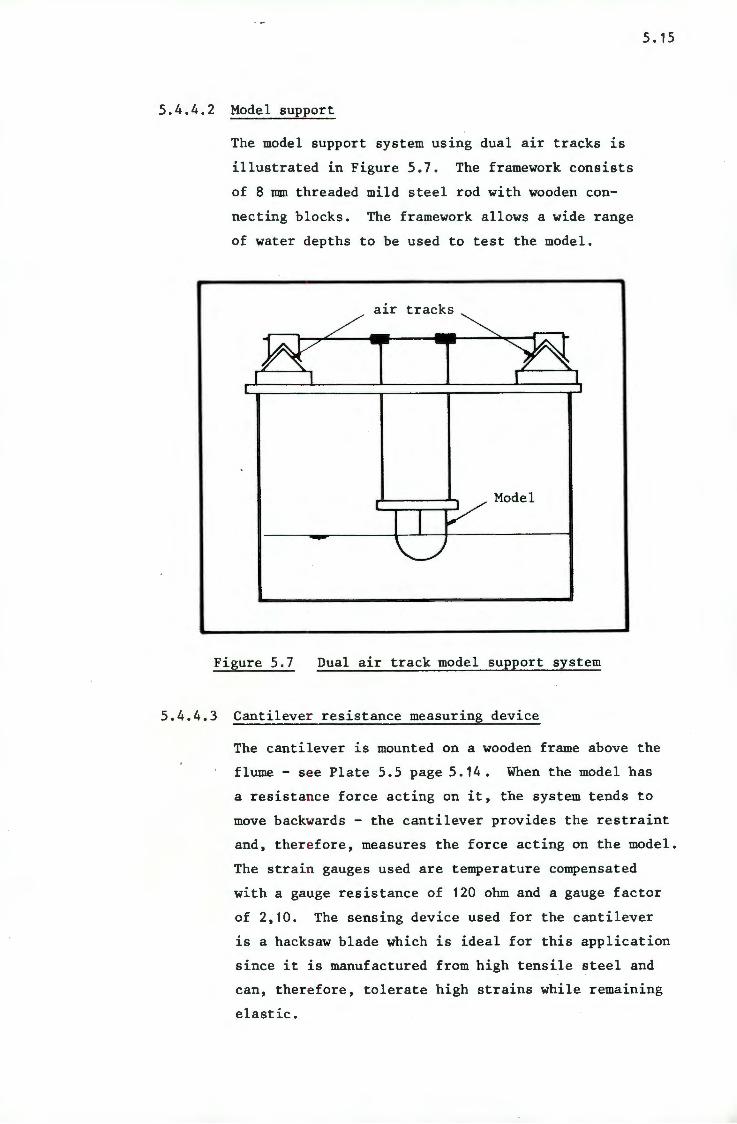
Univers
ity of
Cap
e Tow
n
5.4.4.2 Model support
The model support system using dual air tracks is
illustrated in Figure 5.7. The framework consists
of 8 mm threaded mild steel rod with wooden con
necting bl ocks. The framework allows a wide range
of water depths to be used to test the model.
air tracks
Model
Figure 5.7 Dual air track model support system
5.4.4.3 Cantilever resistance measuring device
5. 15
The cantilever is mounted on a wooden frame above the
flume - see Plate 5.5 page 5.14. When the model has
a resistance force acting on it, the system tends to
move backwards - the cantilever provides the restraint
and, there fore, measures the force acting on the model.
The strain gauges used are temperature compensated
with a gauge resistance of 120 ohm and a gauge factor
of 2,10. The sensing device used for the cantilever
is a hacksaw blade which is ideal for this application
since it is manufactured from high tensile steel and
can, therefore, tolerate high strains while remaining
elastic.
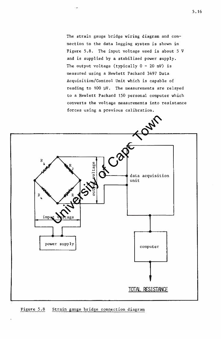
Univers
ity of
Cap
e Tow
n
The strain gauge bridge wiring diagram and con
nect ion to the data logging system is shown in
Figure 5.8 . The input voltage used is about 5 V
and is supplied by a stabilised power supply.
The output voltage (typically 0 - 20 mV) is
measured u s ing a Hewlett Packard 3497 Data
Acquisition/Control Unit which is capable of
reading to 100 µV. The measurements are relayed
to a Hewle t t Packard 150 personal computer which
converts the voltage measurements into resistance
forces using a previous calibration.
--~~~-- data acquisition unit
input voltage
power supply computer
TOTAL RESISTANCE
Figure 5.8 Strain gauge bridge connection diagram
5. 16

Univers
ity of
Cap
e Tow
n
5.4.5 Experimental procedure
5.4.5.1 Calibration of strain gauge bridge
1. The computer, data logger and power supply
must be switched on at least 20 mins before
the s t art of the calibration. This is to
ensure that all the electrical components
have s tabilised before measurements are made.
The s t rain gauge bridge also needs to reach an
equil i brium temperature before readings are
taken . Check that the output voltage of the
power supply to the strain gauge bridge is
approx imately 5 volts.
2. A known force is applied to the cantilever and
the output voltage read by the data logger and
stored in the computer. This procedure is to
be repeated from zero load building up to the
maximum expected load, and then repeated again
going down to zero load to check that there is
no hys teresis in the strain gauge bridge. See
Plates 5.6 and 5.7.
3. The r a tio of the output voltage to the input
voltage is plotted against the applied load.
5. 17
(See Figure 5.9). Using a least squares method
the best fit line is found using the calibration
program. The constants for the slope of the line
and the y-intercept are then used later to cal
culate the total resistance of the model. Note
that t he slope is the most important constant
since it does not change from the calibration
locat i on to the total resistance location. When
calibr ating under zero applied load there is still
the s elf weight of the cantilever acting on the
strain gauge bridge. Therefore, the y-intercept
when measuring the total resistance will be dif
ferent from the y-intercept when calibrating and
this needs to be checked before the start of total
resis t ance measurements.
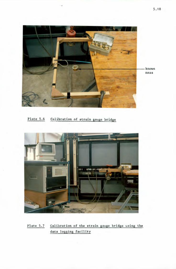
Univers
ity of
Cap
e Tow
n
Plate 5.6
Plate 5.7
5. 18
~~~~~~~~~~~--~~known
Calibration of strain gauge bridge
Calibration of the strain gauge bridge using the
data logging facility
mass
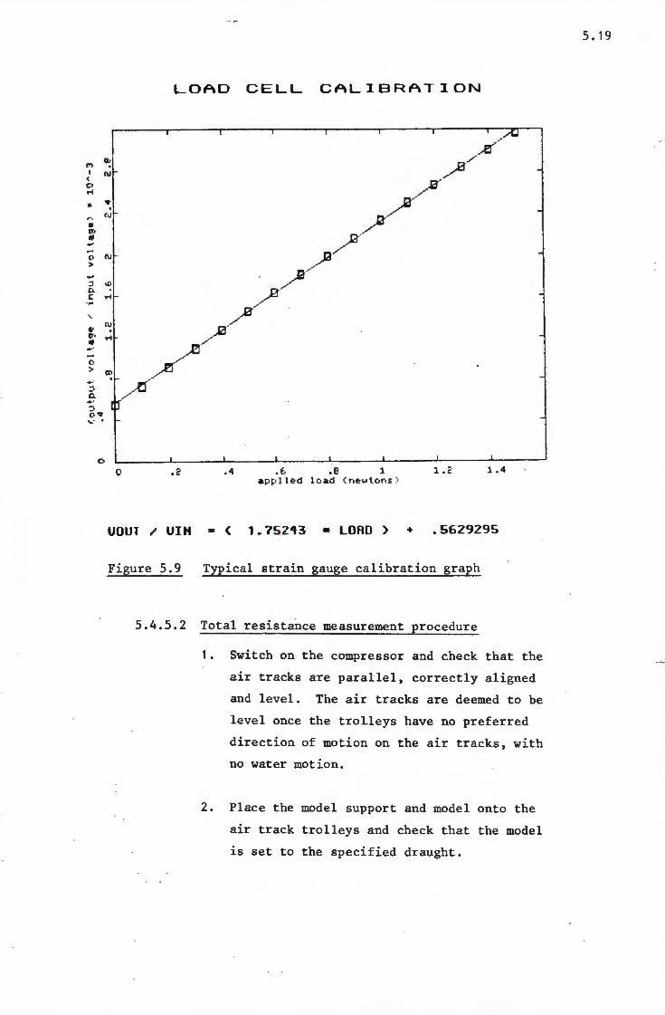
Univers
ity of
Cap
e Tow
n
I') ex. I N < C• ~
• 'It
,. ~ CU .. (ll 1(1 .., -0 N~
>
N •• ~· ~ ....
0
I
LOAD CELL CALIBRATION
I I I
-
-
-
-
-
-
-
I I . . I I I
.2 .4 ,e, .e. 1 1.2 1.4 app l ied load (newtons )
UOUT / UIH £ < 1.75 213 •LORD > + .5629295
Figure 5.9 Typical str ain gauge calibration graph
5.4.5.2 Total resistance measurement procedure
1. Switch on the compressor and check that the
air tracks are parallel, correctly aligned
and level. The air tracks are deemed to be
level once the trolleys have no preferred
direction of motion on the air tracks, with
no water motion.
2. Place the model support and model onto the
air track trolleys and check that the model
is set to the specified draught.
5. 19
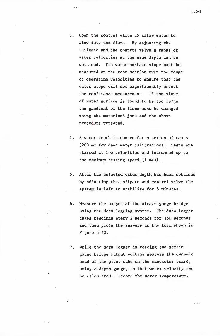
Univers
ity of
Cap
e Tow
n
3. Open t he control valve to allow water to
flow i nto the flume. By adjusting the
tailga te and the control valve a range of
water velocities at the same depth can be
obtained. The water surface slope must be
measur ed at the test section over the range
of operating velocities to ensure that the
water slope will not significantly affect
the r e sistance measurement. If the slope
of wat er surface is found to be too large
the gr .adient of the flume must be changed
using the motorised jack and the above
procedure repeated.
5.20
4. A water depth is chosen for a series of tests
(200 mm for deep water calibration). Tests are
started at low velocities and increased up to
the maximum testing speed (1 m/s).
5. After the selected water depth has been obtained
by adj.usting the tailgate and control valve the
system is left to stabilise for 5 minutes.
6. Measure the output of the strain gauge bridge
us.1ng the data logging system. The data logger
takes readings every 2 seconds for 150 seconds
and then plots the answers in the form shown in
Figure 5.10.
7. While the data logger is reading the strain
gauge bridge output voltage measure the dynamic
head of the pitot tube on the manometer board,
using a depth gauge, so that water velocity can
be calculated. Record the water temperature.

Univers
ity of
Cap
e Tow
n
,., II• c 0 ...
-•• 'O 0 E
a
0
D
0 20
MODEL DRAG v~ TIME
40
a
a
a
0 D a
60 80 100 ti rne <seconds )
a Cb D ifl DD
a a a a a
120 140
D ll:tJ D D a
DATE : 03-07-1986 WATER DEPTH = 200 MM
TIME 19:53:31
WATER TEMPERATURE : 25.2 •c STRAIN GAUGE BRIDGE INPUT VOLTAGE = 5.0108 voHs SLOPE OF LOAD-VOLTAGE LINE =
Y INTERCEPT OF LOAD-VOLTAGE = 1. 75243
.5629295
The drag values are average d between 10.42 and 149.41 seconds. AVERAGE DRAG ~ 1 .272 Newtons VELOCITY = 1 .022 Mis
FigureS.10 Typical total resistance plot
8. Plot the average resistance obtained from the
data logger against the velocity to check that
the readings do not contain gross errors.
9. Increase the water velocity by adjusting the
control valve. Re-set the water height using
the tailgate and go back to step 5 until a
complete curve of total resistance versus
velocity is established,
5.21
Univers
ity of
Cap
e Tow
n
5.5 Measurement of total pressure resistance
To calculate the total pressure resistance of the model the
pressure distribution around the model hull must be established.
To determine the pressure distribution of the model the pressure
at each of the 40 pressure tappings must be measured .
5.5.1 Alternative methods of measuring pressure
Pressure transducers are cormnercially available which will
read the low pressures (typically 500 Pa) acting on the
5.22
model hull. The transducers basically consist of a diaphragm
which has strain gauges mounted on it to form a bridge. Any
deformation of the diaphragm due to an applied pressure causes
a change in the resistance of the strain gauges and conse
quently a change in the output voltage. The pressure trans
ducers have very fast response times typically 0,1 mi l lisecond
which allows reading times to be reduced considerably. The
electrical output of the pressure transducers may also be
measured using the data logging system discussed in Section 5.4.
Pressure transducers are available that read either absolute
pressures or differential pressures.
Another method of measuring pressure is to make use of the
weight of a colt.mm of water. The water is lead from the
pressure tapping into a container of water. To ensure
equilibrium the water level in the container will adjust
to match the pressure at the tapping. If the pressure
fluctuates so will the water level in the container and
hence so will its mass. Therefore, if the mass of the
container is measured it can be interpreted as a pressure
acting at the tapping by using a previous calibration. The
method will have a slow response time to allow for the flow
of water between the container and tapping, but it does have
the advantage of an electrical output that can be measured
using the data logging system.
Univers
ity of
Cap
e Tow
n
5.23
The third method of measuring the pressures is the simplest.
Tubes are led from the pressure tappings to a manometer board
where the changes in water elevation are measured using a
depth gauge. The accuracy that can be obtained by using the
depth gauge to measure the water elevation is 0,1 nnn. The
pressure heads measured by this method are comparable to
points on a hydraulic grade line and, therefore, a reference
to the hull geometry must be made. The disadvantages of this
method are the relatively slow response time and the lack of
electrical output that could be measured using the data logging
system.
5.5.2 Choice of pressure measurement method
Due to the high cos t of the pressure transducers they were
discarded as a choice for pressure measurement. A system
could have been developed using say 2 pressure transducers
and being connected to each tapping in turn, however, the
extra time involved in connecting the hoses would have out
weighed the advantages of the pressure transducers.
Of the other two alternatives it was felt that the manometer
board represented t he simplest and cheapest method of measuring
the pressures. The manometer board does not need any cali
bration and, therefore, is a very pure pressure measurement.
The weighing beaker method is more expensive to manufacture
than the manometer board and the 0,1mm accuracy of the
manometer board would have been difficult to surpass. There
fore, based on cos t , ease of use and simplicity of construction,
the manometer board was chosen as the pressure measurement
method.
5.5.3 Fabrication of the manometer board
The manometer board consists of two sets of 22 glass tubes,
each set mounted on the side of the flume (see Plates 5.8
and 5.9). A depth gauge is mounted above the tubes which
can be moved along to any selected tube. 40 of the glass
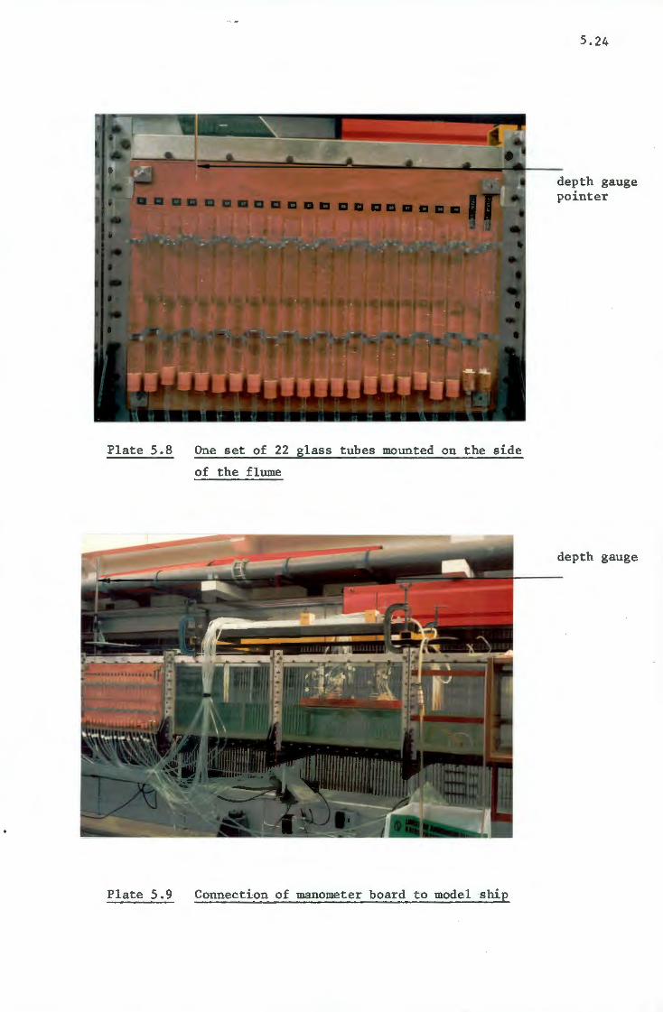
Univers
ity of
Cap
e Tow
n
Plate 5.8
Plate 5.9
One set of 22 glass tubes mounted on the side
of the flume
Connection of manometer board to model ship
5.24
depth gauge pointer
depth gauge

Univers
ity of
Cap
e Tow
n
tubes are used for the pressure tappings, 2 for the
pitot tube, 1 for the upstream tapping and 1 for the
downstream tapping. The upstream and downstream tappings
are used to determine the slope of the water surface as
discussed in Section 5.4.5.
The glass tubes have a 20 mm internal diameter with 1 mm
thi~k wall. The tubes were chosen to have a fairly large
diameter to minimise the effect of capillary rise in the
tubes - see Appendix B.2. Connectors were manufactured
to allow quick connection from the tubes leading from the
hypodermic needles to 8 mm laboratory tubing. The 8 mm
laboratory tubing connects to the glass tube by means of
a rubber bung inserted into the bottom of the glass tube.
5.5.4 Experimental procedure
1. Connect the pressure tappings to their corresponding
glass tubes.
2. By adjusting the tailgate and control valve bring the
water level in the flume up to the specified level.
3. Prime all the pressure tappings and pitot tube hoses.
4. Leave the system to stabilise for 15 minutes.
5. Record the numbers of the tappings that are above the
water surface. Read the water column heights in all
the tappings, repeat again and check for discrepancies.
If there are any discrepancies (i.e. difference in
readings of greater than 0,5 mm) then re-prime the
tapping, wait for 15 minutes and then re-check the
water column height.
6. Take 3 photographs of the water surface profile along
the hull. The one side of the hull has a 10 unn square
grid drawn on a yellow background so that the profile
5.25
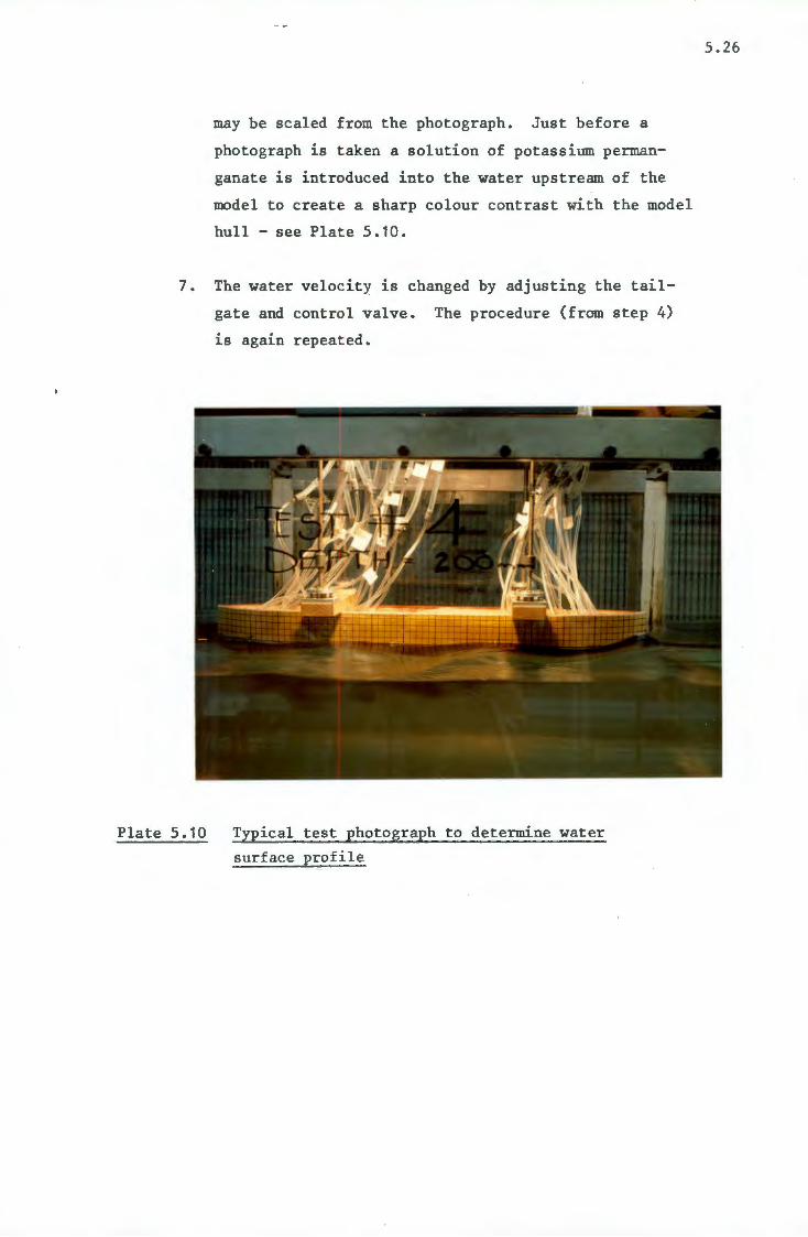
Univers
ity of
Cap
e Tow
n
may be scaled from the photograph. Just before a
photograph is taken a solution of potassium perman
ganate is introduced into the water upstream of the
model to create a sharp colour contrast with the model
hull - see Plate 5.10.
7. The water velocity is changed by adjusting the tail
gate and control valve. The procedure (from step 4)
is again repeat ed.
Plate 5.10 Typical test photograph to determine water
surface profile
5.26
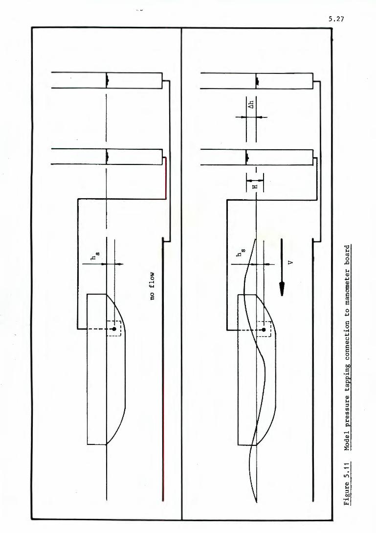
Univers
ity of
Cap
e Tow
n
h s
·~--
-----+
---
no
flo
w
.....-=
•:::
::::....
....
<i
I '
--
I -;r
-_
<..
....
....
....
_ :>
".
F
~
v
Fig
ure
5 .1
1 M
odel
p
ress
ure
tap
pin
g c
on
nec
tio
n
to m
anom
eter
b
oar
d
* l..
n
N .......
Univers
ity of
Cap
e Tow
n
5.28
5.5.5 Calculation. of tot a l pressure resistance
Figure 5.11 illustr ates the connection of one pressure
tapping and the ups tream tapping to the manometer board.
Each tapping on the hull has a defined area dA as i,s
shown in Figure 5. 2 page 5. 6 .
Consider the first case of no flow in the flume shown in
Figure 5 .11. The water level in both the glass tubes will
equal the still water level as shown. The pressure head in
metres of water acting at the tapping will be the sub-
mergence of the tapping below the still water line (i.e. h ).
The value of h is fixed by the geometry of the pressure s
tapping locations.
In the second case where there is flow in the flume the
level in the glass tube connected to the upstream tapping
will remain at the still water level as the tapping has
s
been chosen sufficiently far upstream to be unaffected by
the presence of t he model in the flume. However, the water
level in the glass tube connected to the pressure tapping
will either rise or fall depending on its location on the
hull geometry. Therefore, by comparing the upstream tapping
and pressure tapping readings the value of the change in
water head ~h ac ting on the area dA can be found. By
adding the submergence of the tapping below the still water
level h the pressure head H can be calculated. The s
pressure pgH is multiplied by the area dA to obtain
the normal force acting on the element and then the component
acting in the direction of motion calculated using the angle
the hull surface makes with the direction of motion ¢
The wave profile a long the hull of the model causes some
of the superstruct ure above the still water level to be
wetted and correspondingly, some areas below the still water
line to be exposed . The effect of these changes must be
taken into account when calculating the pressure resistance
of the model. The pressure resistance of the model is
calculated using t he following procedure:
Univers
ity of
Cap
e Tow
n
1. The water surface profile along the model is inter-
k f the water surf ace preted from the photograph ta en o
profile (see Pl ate 5.10 page 5.26). If any area dA
has a portion of its area exposed, the exposed area is
calculated and the area dA correspondingly reduced.
If a
area
pressure tapping is completely exposed, but its
dA sti ll partially wetted, then the wetted area
5.29
is calculated and added to an adjacent tapping (e.g. if
tapping 10 was exposed, its wetted area would be added
to tapping 11's area - see Figure 5.2 page 5.6).
2. The pressure heads H at each tapping are calculated
using the geometry of the pressure tappings
the measured changes in head ~h •
h s
and
3. Pressure distributions around the hull are drawn using
the water surface profile and the pressure heads H •
4. The resis t ance contribution below the still water level
of each tapping is calculated using the following equation
R (below SWL) - pg H dA cos¢ • p
These contributions are added to obtain the resistance
contribution of the hull below the still water level -
ER (be low SWL). p
5. The length of the superstructure is divided into segments.
From the pressure distribution diagrams the average
pressur e in metres of water h and the area over which a it acts is calculated for each segment. For each seg-
ment i t s contribution to the total pressure resistance
is calculated
R (above SWL) = pg h A cos¢ p a
These contributions are addded to obtain the resistance
contribution of the hull above the still water level -
E R (above SWL) • p
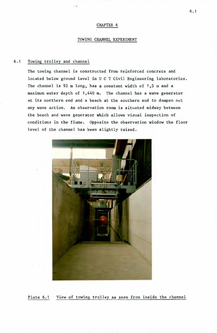
Univers
ity of
Cap
e Tow
n
CHAPTER 6
TOWING CHANNEL EXPERIMENT
6.1 Towing trolley and channel
The towing channel is constructed from reinforced concrete and
located below ground level in U C T Civil Engineering laboratories.
The channel is 92 m long, has a constant width of 1,5 m and a
maximum water depth of 1,440 m. The channel has a wave generator
at its northern end and a beach at the southern end to dampen out
any wave action. An observation room is situated midway between
the beach and wave generator which allows visual inspection of
conditions in the flume. Opposite the observation window the floor
level of the channel has been slightly raised.
Plate 6. 1 View . of towing trolley as seen from inside the channel
6.1
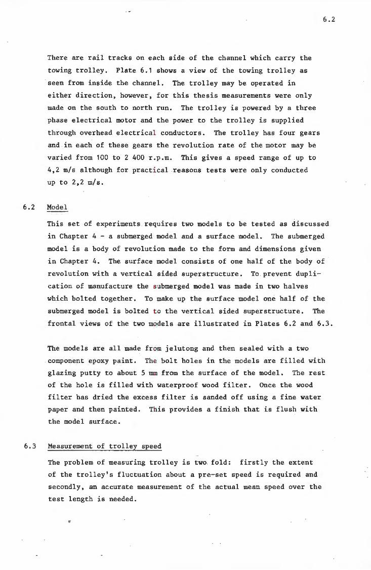
Univers
ity of
Cap
e Tow
n
There are rail tracks on e ach side of the channel which carry the
towing trolley. Plate 6.1 shows a view of the towing trolley as
seen from inside the channe l. The trolley may be operated in
either direction, however, for this thesis measurements were only
made on the south to north run. The trolley is powered by a three
phase electrical motor and the power to the trolley is supplied
through overhead electrical conductors. The trolley has four gears
and in. each of these gears the revolution rate of the motor may be
varied from 100 to 2 400 r .p.m. This gives a speed range of up to
4,2 m/s although for practi cal reasons tests were only conducted
up to 2,2 m/s.
6.2 Model
6.2
This set of experiments requires two models to be tested as discussed
in Chapter 4 - a submerged model and a surface model. The submerged
model is a body of revolut i on made to the form and dimensions given
in Chapter 4. The surface model consists of one half of the body of
revolution with a vertical sided superstructure. To . prevent dupli
cation of manufacture the submerged model was made in two halves
which bolted together. To make up the surface model one half of the
submerged model is bolted t o the vertical sided superstructure. The
frontal views of the two models are illustrated in Plates 6.2 and 6.3.
The models are all made fr om jelutong and then sealed with a two
component epoxy paint. The bolt holes in the models are filled with
glazing putty to about 5 Dllil from the surface of the model. The rest
of the hole is filled with waterproof wood filter. Once the wood
filter has dried the excess filter is sanded off using a fine water
paper and then painted. Th is provides a finish that is flush with
the model surface.
6.3 Measurement of trolley speed
The problem of measuring trolley is two fold: firstly the extent
of the trolley's fluctuation about a pre-set speed is required and
secondly, an accurate measurement of the actual mean speed over the
test length is needed.
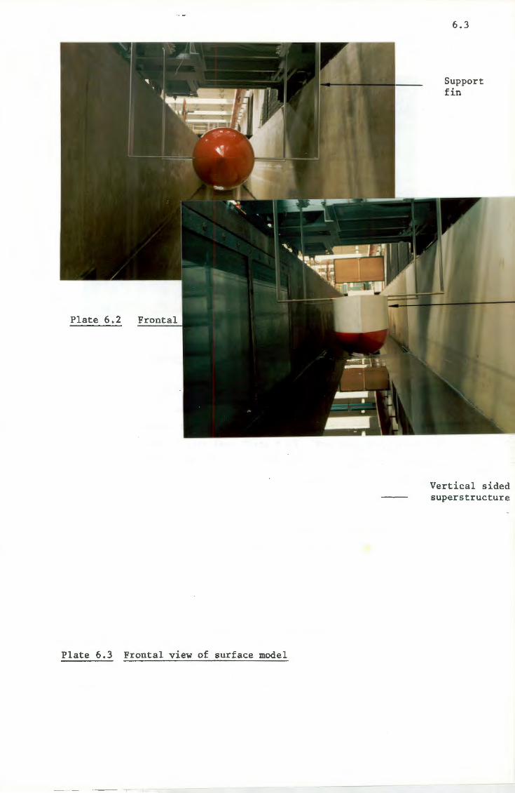
Univers
ity of
Cap
e Tow
n Plate 6.2 Frontal
Plate 6.3 Frontal view of surface model
-- T'"
6 . 3
Support fin
Vertical sided superstructure
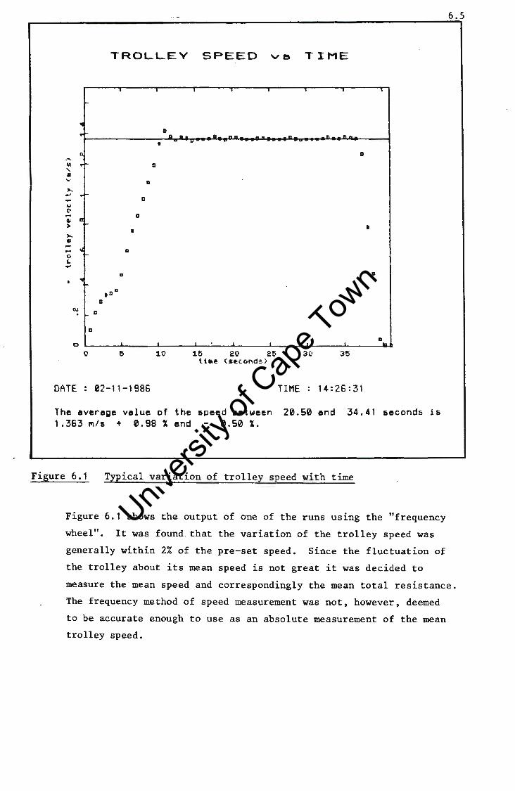
Univers
ity of
Cap
e Tow
n
6.5
TROLLEY SPEED ve TIME
D
• a
Ul D
' Ii .... D ,.., .,.,
D .., (I
a ti >
I I
,..., ti
D 0 '-.,.,
D D
,ac a
(\I D
D
D 0
0 10 15 20 25 35 t.h;e <secon ds )
DATE : 02-11-1986 TI ME : 14 : 2 6 : 31
The average velue of the speed between 20.50 end 34.41 seconds is 1 .363 ~/s + 0.98 X and 0.50 1.
Figure 6.1 Typical variation of trolley speed with time
Figure 6.1 shows the output of one of the runs using the "frequency
wheel". It was found . that the variation of the trolley speed was
generally within 2% of the pre-set speed. Since the fluctuation of
the trolley about its mean speed is not great it was decided to
measure the mean speed and correspondingly the mean total resistance.
The frequency method of speed measurement was not, however, deemed
to be accurate enough to use as an absolute measurement of the mean
trolley speed.
Univers
ity of
Cap
e Tow
n
To measure the mean speed accurately (to within 1%) an electronic
timer capable of reading t o 0,1 milliseconds is used. The timer
is activated using a micro switch at the start of the test section
and then again stopped by another micro switch at the end of the
6.6
test section . The length of the test section is accurately measured
using a steel tape. Thus, in this way, very accurate ~easurements of
the mean speed of the trol l ey may be made.
6.4 Measurement of total resis t ance
6.4.1 Total resistance mea surement system
The choices and prob lems for the measurement system are
essentially the same as for the glass flume experiments.
The only problem uni que to the towing channel experiment is
the measurement of t he total resistance of the submerged
model.
The submerged model must be supported in some way, and when
the total resistance of the model is measured the resistance
of the support structure must not be included in the measure
ment. One way to achieve this would be to place the load
sensing device inside the model so that only the model
resistance would be measured. The support structure would
still, however, interfere with the flow around the model and
this effect would be difficult to quantify. In addition,
placing the load sensing devices under water introduces extra
problems of waterproofing.
Consider the model shown in Figure 6.2 supported on either
side by a strut. I f the resistance of the model is measured
with both struts in place the measured resistance would be
the model resistance Rm plus two strut resistances 2RST .
If one of the sets of struts is now removed the measured
resistance would be Rm + RST .
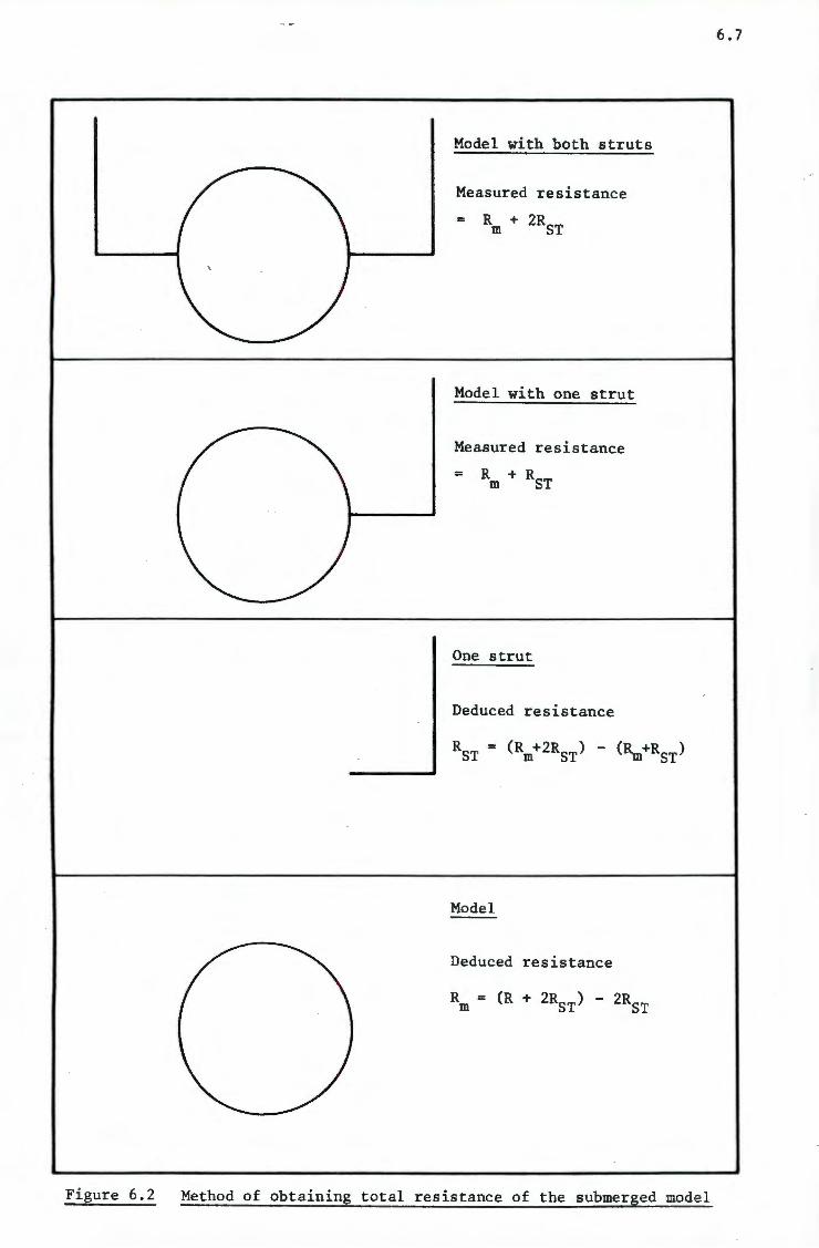
Univers
ity of
Cap
e Tow
n
Figure 6.2
Model with both struts
Measured resistance
=
Model with one strut
Measured resistance
= Rm + RST
One strut
Deduced resistance
Model
Deduced resistance
Method of obtaining total resistance of the submerged model
6.7
Univers
ity of
Cap
e Tow
n
By subtracting the second measurement from the first
measurement the resistance due to one strut, RST can
be found. Now twice the strut resistance 2RST sub
tracted from the first measurement (Rm + 2RST) will
give the resistance of the model R m
This method
provides an elegant and pure method of obtaining the
submerged resistance of the model without positioning
the load measuring device under water.
The use of an air t r ack to support the model on the
trolley would have r equired a relatively large air flow
to lift the mass of the model. An air compressor would
have to be mounted on the trolley to supply the required
air flow. Since a compressor that could deliver the
required air flow was not available the use of the air
track as a support method was not possible.
Thus the rolling bearing support method was chosen to
support the framework. The framework was designed bearing
in mind that one set of struts would have to be removed
later in the experimental work. To measure the resistance
force acting on the model a strain gauge bridge .is used.
6.4.2 Fabrication of total resistance measurement system
6.4.2.1 Support framework
Plate 6.5 shows the support framework on the
trolley with the submerged model in position.
The framework is made from 60 x 40 x 4 mm box
sections and the struts from 80 x 8 mm flat
sections. The struts below the water line are
streamlined to the profile shown in Figure 6.3.
6.8
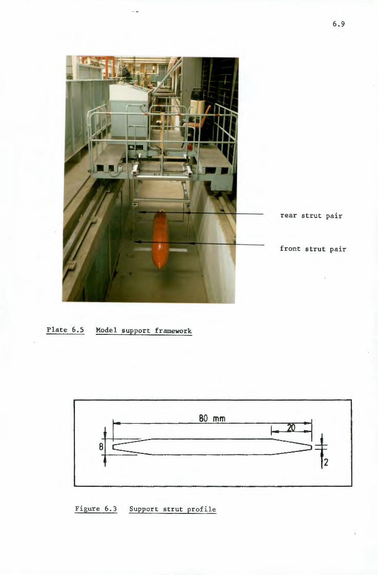
Univers
ity of
Cap
e Tow
n
6.9
rear strut pair
front strut pair
Plate 6.5 Model support framework
80 mm
Figure 6.3 Support strut profile
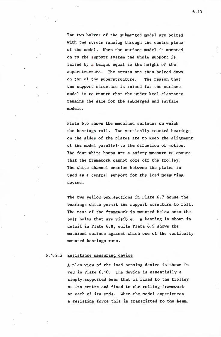
Univers
ity of
Cap
e Tow
n
The two hal ves of the submerged model are bolted
with the s t ruts running through the centre plane
of the mode l. When the surface model is mounted
on to the support system the whole support is
raised by a height equal to the height of the
superstruct ure. The struts are then bolted down
on top of t he superstructure. The reason that
the suppor t structure is raised for the surface
model is t o ensure that the under keel clearance
remains the same for the submerged and surface
models.
Plate 6.6 shows the machined surfaces on which
6. 10
the bearings roll. The vertically mounted bearings
on the side s of the plates are to keep the alignment
of the mode l parallel to the direction of motion.
The four white hoops are a safety measure to ensure
that the framework canno.t come off the trolley.
The white channel section between the plates is
used as a central support for the load measuring
device.
The two yellow box sections in Plate 6.7 house the
bearings which permit the support structure to roll.
The rest of the framework is mounted below onto the
bolt holes that are visible. A bearing is shown in
detail in Plate 6.8, while Plate 6.9 shows the
machined surface against which one of the vertical l y
mounted bearings runs.
6.4.2 . 2 Resistance measuring device
A plan view of the load sensing device is shown in
. red in Plate 6.10. The device is essentially a
simply supported beam that is fixed to the trolley
at its centre and fixed to the. rolling framework
at each of its ends. When the model experiences
a resisting force this is transmitted to the beam.
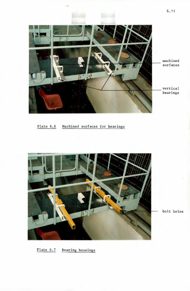
Univers
ity of
Cap
e Tow
n
Plate 6.6 Machined surfaces for bearings
Plate 6.7 Bearing housings
6. 11
machined surfaces
vertical bearings
bolt holes
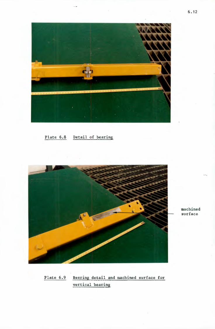
Univers
ity of
Cap
e Tow
n
Plate 6.8
Plate 6.9
Detail of bearing
Bearing detail and machined surface for
vertical bearing
6. 12
machined surface
Univers
ity of
Cap
e Tow
n
The maximum bending occurs at the centre of the
beam and for this reason the strain gauges are
mounted on e ither side of the central support.
On the left hand side of Plate 6.10 a hook is
visible; this hook is used to calibrate the strain
gauge bridge . Plate 6.11 illustrates how a known
mass is app l ied to the framework through a cable
from which t he mass is suspended.
6. 13
Once tests were started it was found that the output
of the strai n gauge bridge had an alternating voltage
component. This was caused chiefly through the
trolley not being able to maintain a completely
uniform speed. Attempts to dampen the motion of
the framewor k proved fruitless because of the
relatively small resistance forces involved. Thus
to solve the problem electrical damping was used.
A simple fi r st order low pass filter was made with
a resistor value of 1 800 ohm and a capacitor value
of 1. 470 micro farad. The filter has a response time
of about 4 seconds to reach 95% of the true value.
Since all t he run times were in excess of 10 seconds
the delay wa s not significant. The theory behind the
low pass fi l ter is discussed in Appendix C.
The output voltage of the strain gauge bridge is read
using a char t recorder and the resistance force inter
preted using a previous calibration.
6.4.3 Experimental procedur e
All runs are from the south end of channel to the north end
and no readings- are t aken on the return run.
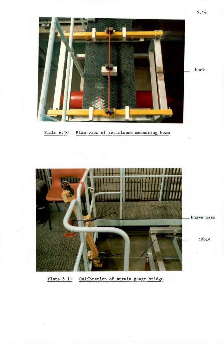
Univers
ity of
Cap
e Tow
n
6. 14
hook
Plate6.10 Plan view of resistance measuring beam
known mass
cable
Plate 6.11 Calibration of strain gauge bridge

Univers
ity of
Cap
e Tow
n
At the start of each run the strain gauge is calibrated on
the chart recorder ( see Figure 6.4). This sets the scale
for the resistance t i me plot. Once the calibration 1s
complete the run is s tarted and the total resistance
variation plotted us i ng the chart recorder as shown in
Figure 6.4. The time interval is recorded and the speed
calculated.
The return run 1s done at approximately the same speed as
the live run. About 5 to 20 minutes are required before
the start of the next run to allow wave action and water
currents to die down. This time period is dependent on
the speed of theprevious run. The water temperature is
recorded every hour when tests are being conducted.
The total resistance is scal~d from the resistance time plot
and then plotted against speed.
To obtain the hull water surface profile for the surface
model photographs are taken from the observation room (see
Plate 6.12).
Plate 6.12 Photograph . of hull water surface profile
6. 15
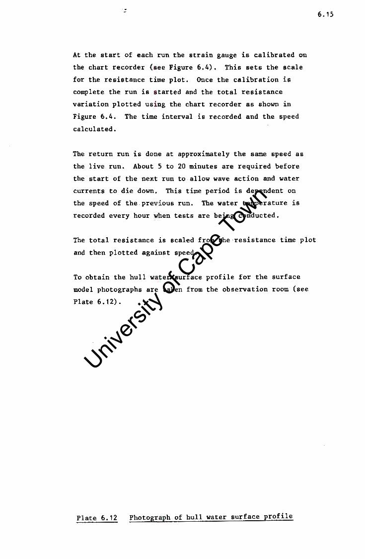
Univers
ity of
Cap
e Tow
n
At the start of each run the strain gauge is calibrated on
the chart recorder ( see Figure 6.4). This sets the scale
for the resistance t i me plot. Once the calibration is
complete the run is .s tarted and the total resistance
variation plotted us i ng the chart recorder as shown in
Figure 6.4. The time interval is recorded and the speed
calculated.
The return run is done at approximately the same speed as
the live run. About 5 to 20 minutes are required before
the start of the next run to allow wave action and water
currents to die down . This time period is dependent on
the speed of the previous run. The water temperature is
recorded every hour when tests are being conducted.
The total resistance is scal~d from the resistance time plot
and then plotted agai nst speed.
To obtain the hull water surface profile for the surface
model photographs are taken from the observation room (see
Plate 6. 12) •
Plate 6.12 Photograph of hull water surf ace profile
6. 15
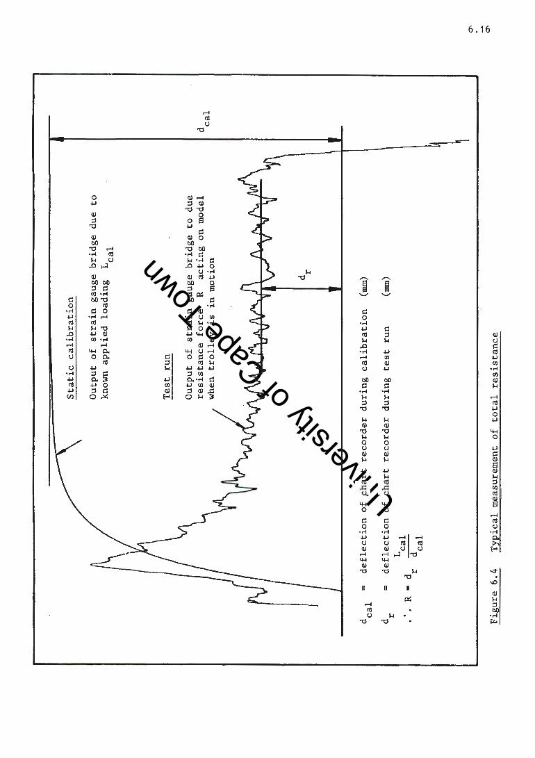
Univers
ity of
Cap
e Tow
n
d cal
=
d =
r
R =
d
Sta
tic c
ali
bra
tio
n
Ou
tpu
t o
f str
ain
gau
ge
bri
dg
e d
ue
to
know
n ap
pli
ed
lo
ad
ing
L
1
ca
Test
ru
n
Ou
tpu
t o
f str
ain
gau
ge
bri
dg
e
to
du
e re
sist
an
ce
forc
e
R
acti
ng
on
mod
el
whe
n tr
oll
ey
is
in
mo
tio
n
d r
defl
ecti
on
of
ch
art
re
co
rder
du
rin
g cali
bra
tio
n
(mm
)
defl
ecti
on
of
ch
art
re
co
rder
du
rin
g te
st
run
(n
un)
L cal
r -d
-cal
Fig
ure
6
.4
Ty
pic
al m
easu
rem
ent
of
tota
l re
sist
an
ce
d cal
°' °'
Univers
ity of
Cap
e Tow
n
To ensure that the submerged model was deeply submerged,
checks were made a t higher speeds to ensure that the
submerged model did not generate a set of waves at the
water surface. Thi s was done at speeds of up to 2,2 m/s
and no evidence of waves due to the model were noted.
6.17
The sequence of te s ting was first the submerged model with
both sets of suppor t fins, then the surface model and, finally,
the submerged mode l with one set of support fins removed.
Figure 6.5 shows a plan view of the submerged model and support
fins. When testing the submerged model with one set of support
fins removed, the i deal set to remove would be A and B, or
C and D. To achieve this, however, the strength of the support
fins would have to be increased leading to a larger fin cross-
section. Therefore , fins A and D were removed which allowed
the fin cross-sect i on to remain relatively small. The two sets
of fins (AC and BD) are relatively far apart and thus it is
unlikely that the l eading fin will influence the trailing fin,
therefore~ removing support fins A and D is hydraulically
equivalent to remov ing A and B.
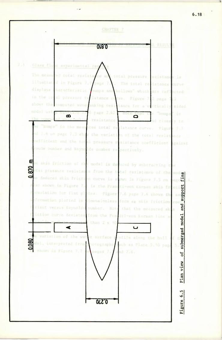
Univers
ity of
Cap
e Tow
n
6. 18
Cfl i::
·.-j
4-1
µ j..j
0 0.
::I Cfl
"O i:: Ill
r-4 Q)
"O 0 s
u "O Q)
00 j..j Q)
s ,J:l ::I Cl)
4-1 0
~ Q)
·.-j
:> i:: Ill
r-4 p...
1.1"'1 . \Cl
Oll 0 Q) j..j
::I 00
·.-j
lJ:.<
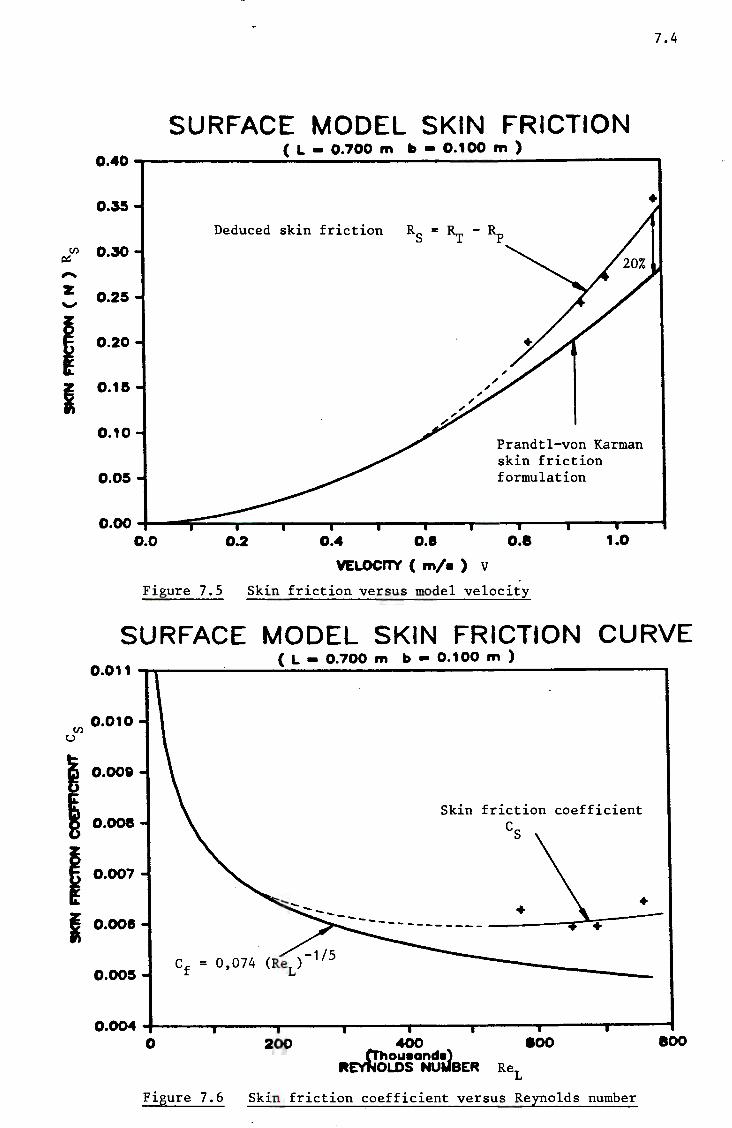
Univers
ity of
Cap
e Tow
n
ti)
p:: ,... z -I I
ti)
u
~ 0
I I I
0.40
o.~
0.30
0.2S
0.20
O.t&
O.to
o.os
o.oo o.o
SURFACE MODEL SKIN FRICTION ( L - o. 700 m b - · O. t 00 m )
Deduced skin friction
0.2
Prandtl-von Karman skin friction formulation
o.4 o.e o.e t.O VELOCITY ( m/e ) V
Figure 7.5 Skin f riction versus model velocity
7.4
•
SURFACE MODEL SKIN FRICTION CURVE ( L - _ O. 700 m b - O. 1 00 m )
0.011 --.--~~--~~..;....~--~~~~~~~~~~~----~~~ .....
0.010
0.009
Skin friction coefficient 0.008 cs
0.007
+ + o.ooe
-1/5 o.oos Cf = 0,074 (ReL)
0 400 eoo trho"eand•)
llt~OLDS NU.ieER ReL
800 200
Figure 7.6 Skin friction coefficient versus Reynolds number
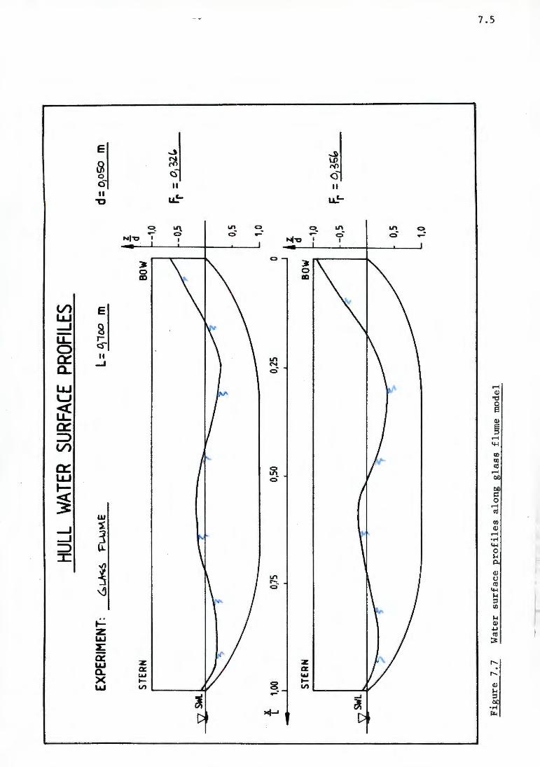
Univers
ity of
Cap
e Tow
n
HULL
W
ATER
SU
RFAC
E PR
OFIL
ES
EXPE
RIM
ENT:
6.L
..11<
6 Fi..w~e
L= 0
110
0
m
STER
N
BOW
A l
1,00
0,7
5 0,
50
0,25
0
STER
N
BOW
Fig
ure
7
.7
Wat
er
surf
ace p
rofi
les
alo
ng
g
lass
fl
ume
mod
el
~
-
d:
010
SO
m
z d -1,0
-o.s
Fr =
o, 32
£,,
0,5
1,0
•• d -1,0
-o,5
Fr
= D, ~;
"
0,5
1,0
-...J
VI
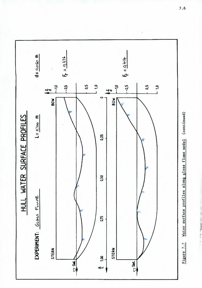
Univers
ity of
Cap
e Tow
n
HULL
W
ATER
SU
RFAC
E PR
OFI
LES
EXPE
RIM
ENT:
Gt
...~
F
!AA
r\E
. L=
011
00
m
d
: 0
10~ m
z
STER
N
BOW
.d
-1,0
-0,5
Fr
= o,
~7~
0,5
1,0
t 1,
00
0,75
0,
50
0,25
0
I .I.
d
STER
N
BOW
-1
,0
-o,5
Fr
= o,
4-t It
'5
0,5
1,0
-....J
Fig
ure
7
.7
Wat
er
surf
ace
pro
file
s al
on
g g
lass
fl
ume
mod
el
(co
nti
nu
ed)
. "'
--
--ir
··-· "
" .,..
.--
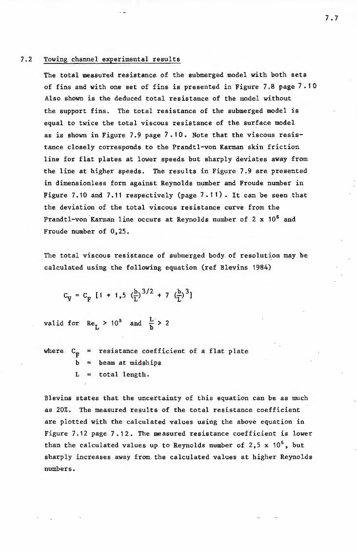
Univers
ity of
Cap
e Tow
n
7.2 Towing channel experimental results
The total measured resistance of the submerged model with both sets
of fins and with one set of fins is presented in Figure 7 .8 page 7. 1 0
Also shown is the deduced t otal resistance of the model without
the support fins. The tota l resistance of the submerged model is
equal to twice the total viscous resistance of the surface model
as 1s shown in Figure 7.9 page7.10. Note that the viscous resis
tance closely corresponds t o the Prandtl-von Karman skin friction
line for flat plates at lower speeds but sharply deviates away from
the line at higher speeds. The results in Figure 7.9 are presented
in dimensionless form against Reynolds number and Froude number in
Figure 7. 10 and 7. 11 respectively (page 7 • 1 1) • It can be seen that
the deviation of the total viscous resistance curve from the
Prandtl-von Karman line occurs at Reynolds number of 2 x 10⁶ and
Froude number of 0,25.
The total viscous resistance of submerged body of resolut~on may be
calculated using the following equation (ref Blevins 1984)
valid for
where = = =
and
resistance coefficient of a flat plate
beam at midships
total lengt h.
Blevins states that the uncertainty of this equation can be as much
as 20%. The measured re sults of the total resistance coefficient
are plotted with the calculated values using the above equation in
Figure 7.12 page 7 .12. The measured resistance coefficient is lower
than the calculated values up to Reynolds number of 2,5 x 10⁶, but
sharply increases away from the calculated values at higher Reynolds
numbers.
7. 7
Univers
ity of
Cap
e Tow
n
7.8
Figure 7.13 page 7 .13 shows the resistance coefficient of the model
based on frontal area plotted against Reynolds number based on model
diameter R~ . Also shown are the resistance coefficient curves
for a sphere and disc (from Vennard 1976), and the resistance
coefficient of the submerged model calculated using Blevins' method.
The variation in the resis tance coefficient of the sphere is due to
the size of the wake and t he nature of the boundary layer. The
resistance coefficient of the disc shows no variation with Reynolds
number, as the separation point is fixed regardless of the nature
of the boundary layer (i.e. the width of the wake remains constant
and, therefore, the resis tance coefficient remains constant). There
fore, it seems that the i ncrease in the measured resistance coef
ficient of the model above ReD of 2,5 x 10 5 is due to an increase
in the size of the wake.
The measured total resistance of the surface model is shown in
Figure 7.14 page 7.14. Also plotted is the total viscous resistance
obtained from the submer ged model. By subtracting the total viscous
resistance from the tot al resistance, the wave-making resistance of
the model can be deduced as shown in Figure 7.14. The deduced wave
making resistance is plotted with the calculated wave-making resistance
in Figure 7.14 page 7.1 4 . It is evident that the magnitude of the
first few "humps" was t oo small to be measured. However, there is a
fairly good correlation with the one peak shown although the magni
tude of the measured value is greater than the calculated value.
Figure 7.16 page 7.15 shows the variation of the total resistance
coefficient with Froude number, while Figure 7.17 page 7.15 shows
the variation of the wave-making resistance coefficient with Froude
number.
The hull water surface profiles for a range of Froude numbers are
illustrated in Figure 7.18 on page 7.16 to 7.18, derived from
photographs (e.g. Plate 6.12 page 6.15).
Univers
ity of
Cap
e Tow
n
Consider the case of a body of revolution (such as submarine)
rising from being deeply submerged to the surface of a fluid.
When the body is deeply submerged it will have viscous resistance
and no wave-making resist ance, at the surface the body will
generate waves and have v i scous resistance although the surface
area of the body in contact with the fluid has decreased.
Figure 7.19 page 7.19 illustrates the resistance variation of
the model as it rises through the surface. Notice that the
maximum resistance occurs just before the model breaks the surface,
i.e. when the model's sur face area is stiH completely wetted and
yet near enough to the surface to generate waves.
7. 9
I
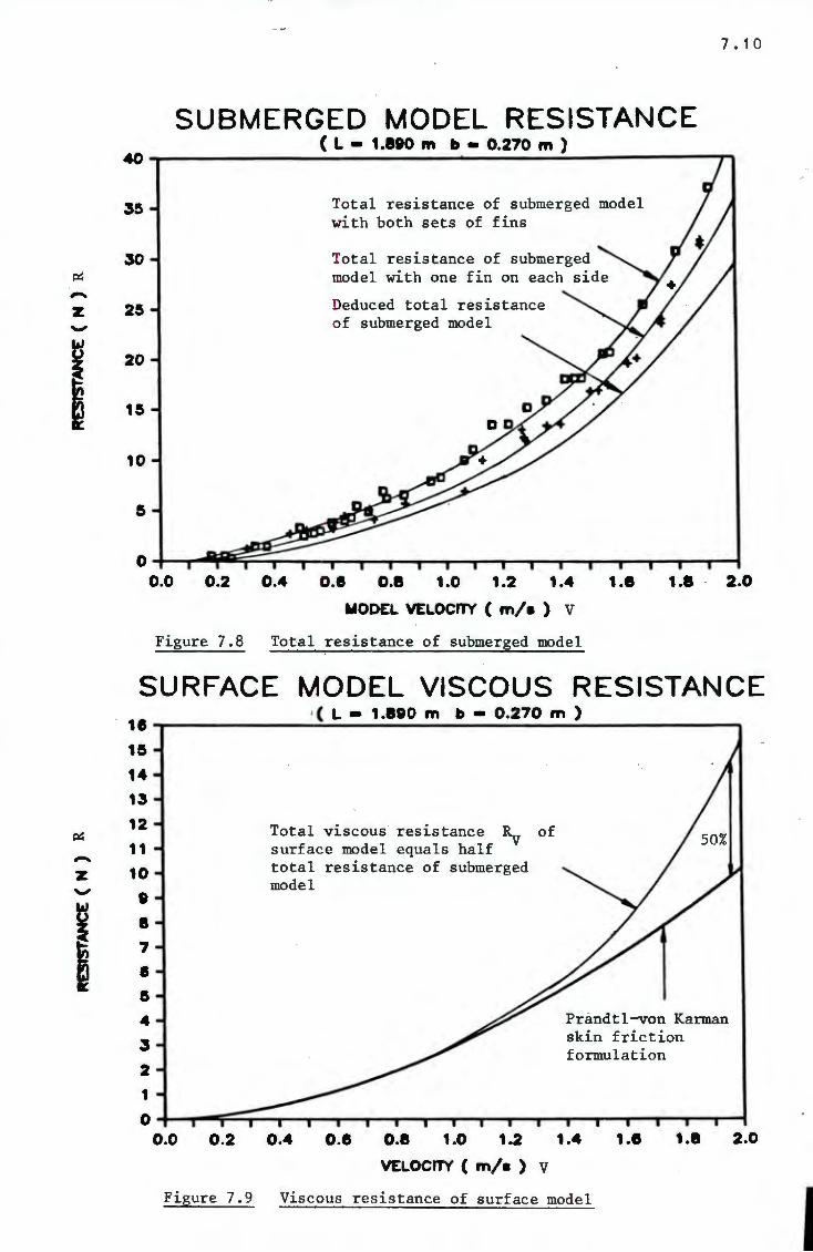
Univers
ity of
Cap
e Tow
n
-z -I
~ -z -I
7 • 1 0
SUBMERGED MODEL RESISTANCE ( L • 1.190 m b • 0.270 m )
40--------------------------------------...;...------------~n
30
2&
20
1&
10
Total resistance of submerged model with both sets of fins
Total resistance of submerged model with one fin on each side
Deduced total resistance of submerged model
o.o 0.2 0.4 o.e o.8 1 .o 1.2 1 .4 1.e 1.8 2.0
MODEL VELOCITY ( m/a ) V
Figure 7.8 Total resistance of submerged model
SURFACE MODEL VISCOUS RESISTANCE 18
1&
14
13
12
11
10
' 8
7
e s 4
3
2
1
0 o.o 0.2
1 ( L - 1 .890 m b • 0.270 m )
Total viscous resistance ~ of surface model equals half total resistance of submerged model
Prandtl-von Karman skin friction formulation
0.4 o.e o.8 1 .o 1 .2 1.4 VELOCITY ( m/a ) V
1.e 1.8
Figure 7.9 Viscous resistance of surface model
2.0
I
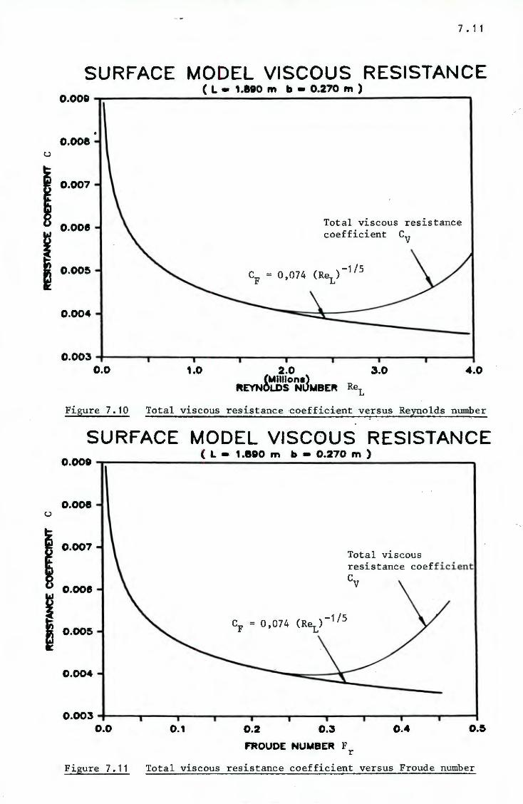
Univers
ity of
Cap
e Tow
n
u
7 • 1 1
SURFACE MODEL VISCOUS RESISTANCE ( L • 1.890 m b • 0.270 m )
0.001-----------------------------------------------------,
o.ooe
0.007
o.ooe Total viscous resistance coefficient CV i I o.oos
u
0.004
0.003-.--------------...-----------------------------------------1 o.o 1.0 2.0 3.0
(Mllllone) REYNOLDS NUMBER Re1
4.0
Figure 7.10 Total viscous resistance coefficient versus Reynolds number
SURFACE MODEL VISCOUS RESISTANCE ( L • 1 .890 m b • 0.270 m )
0.009------------------------------------------------------
o.ooe
0.007
o.ooe
Total viscous resistance coefficient CV
i I o.oos CF = 0,074
0.004
0.003-.------r---------...-----...----------..-----.-----.-----..-----1 o.o 0.1 0.2 0.3
FROUDE NUMBER F r
0.4 O.&
Figure 7.11 Total viscous resistance coefficient versus Froude number
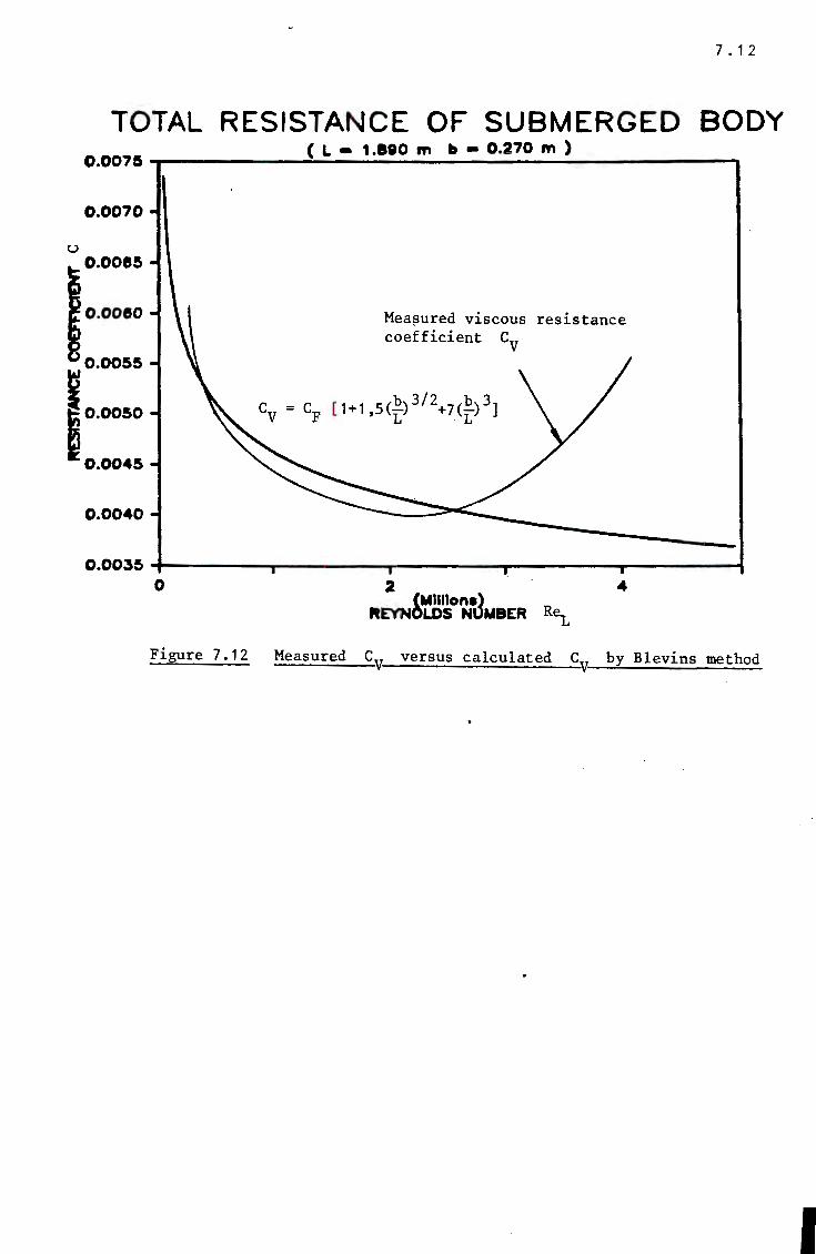
Univers
ity of
Cap
e Tow
n
7 • 1 2
TOTAL RESISTANCE OF SUBMERGED BODY 0.007S
0.0070
u 0.0085
o.ooeo
0.0055 I 0.0050
0.0045
0.0040
0.0035 0
Figure 7.12
( L - 1 .890 m b • 0.270 m )
Mea~ured viscous resistance coefficient CV
2 4 (Mllllone)
ftEYNOLDS Nl>MBER R~
_M_ea_s_u_re_d ___ cv versus calculated CV by Blevins method
I
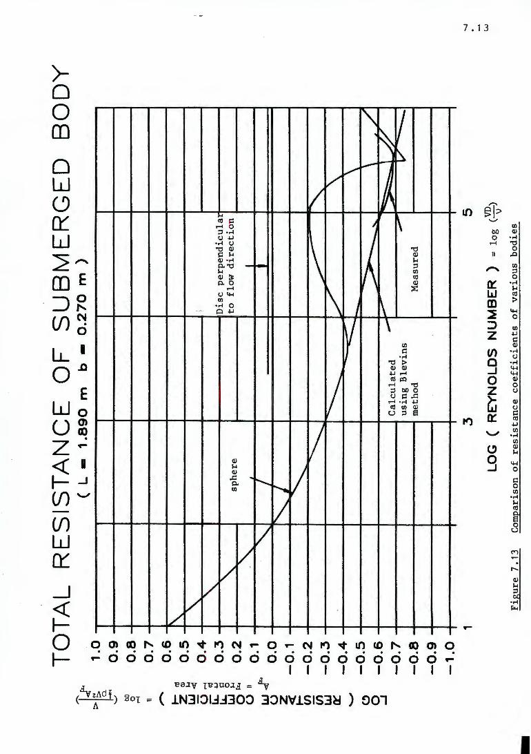
Univers
ity of
Cap
e Tow
n
TO
TA
L
RE
SIS
TA
NC
E
OF
S
UB
ME
RG
ED
B
OD
Y
( L
-1
.89
0
m
b -
0.2
70
m
)
r.-.
~
1.0
:>
IS.
0.
-«'<
0.9
'-
'
bO
0.8
0 ....4
0.7
~
0.6
t-
c1'
0.5
z
~
~~
0.4
01
"'4
-c1'
LL~
0.3
LL
i:::
UJ
~
0.2
o~
U
II 0
.1
UJ~
0.0
u z
-0.1
~ (/
) -0
.2
(/)
-0.3
UJ
0:
: -0
.4
......,
(.!)
-0
.5
0 -0
.6
_J
-0.7
\. "'
'
" "' D
isc
per
pen
dic
ula
L
sph
ere
to
flo
w d
irecti
on
.~
I I
"' I
t
""-
I "' ~
~
" ~
I_
/
'\
--.......
.... -
\ ~ ..
. l
~/
----~
-~
Cal
cula
ted
u
sin
g B
lev
ins
-v
----
-0.8
m
etho
d M
easu
red
-0.9
-1
.0
1 3
5 "
LOG
(
RE
YN
OL
DS
N
UM
BE
R
) =
lo
g (~)
w
Fig
ure
7.1
3
Com
pari
son
of
resi
stan
ce c
oeff
icie
nts
o
f v
ari
ou
s b
od
ies
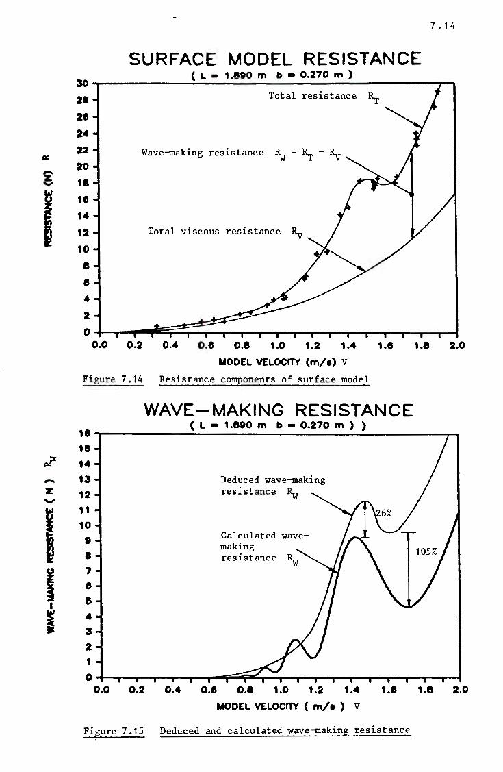
Univers
ity of
Cap
e Tow
n
p::
g
I
~
-z -I I I
~ •
7. 1 4
SURFACE MODEL RESISTANCE 30
( L - 1 .890 m b • 0.270 m )
28
2e
24
22 Wave-making resistance ~ = Rr - l\r 20
11
11
14
12 Total viscous resistance
10
I
I
4
2
0 o.o 0.2 o.4 o.e 0.1 1.0 1.2 1.4 1.e
MODEL VELOCfTY {m/a) V
Figure 7.14 Resistance components of surface model
11
1&
14
13
12
" 10
8
• 7 e a 4
3
2 1
0 o.o
WAVE-MAKING RESISTANCE
0.2 0.4
( L - 1.890 m b - 0.270 m ) )
Deduced wave-making resistance ~
Calculated wavemaking resistance ~
o.e 0.1 1.0 1.2 1.4
MODEL VELOCfTY { m/ e ) V
1.e
Figure 7.15 Deduced and calculated wave-making resistance
1.8 2.0
1.8 2.0
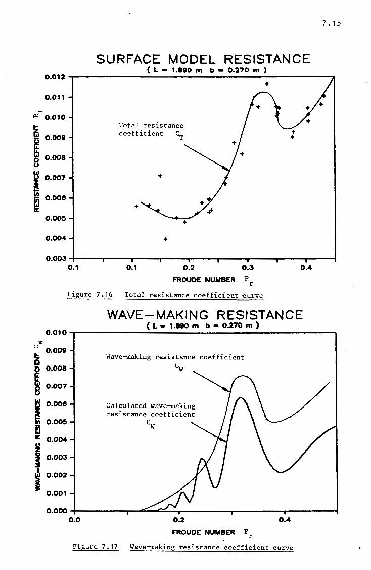
Univers
ity of
Cap
e Tow
n
0.012
0.011
~ 0.010
~ 0.009
~ 0.008
~ 0.007
~ 0.006
~ 0.005
0.004
0.003
0.010 :;3:
u 0.009
~ 0.008
~ 0.007 8 ..... o.ooe
~ 0.005 Ei ~ 0.004 ~
I 0.003
I 0.002
~ • 0.001
o.ooo
SURFACE MODEL RESISTANCE
0.1
( L • 1.890 m b - 0.270 m )
Total resistance coefficient CT
+
+
+
+
0.1 0.2 0.3
FROUDE NUMBER Fr
Figure 7.16 Total r esistance coefficient curve
0.4
WAVE-MAKING RESISTANCE
0 .0
( L • 1.890 m b • 0.270 m )
Wave-making resistance coefficient cw
Calculated wave-making resistance coefficient
cw
0.2
FROUDE NUMBER F r
0.4
Figure 7.17 Wave-making resistance coefficient curve
7 • 15
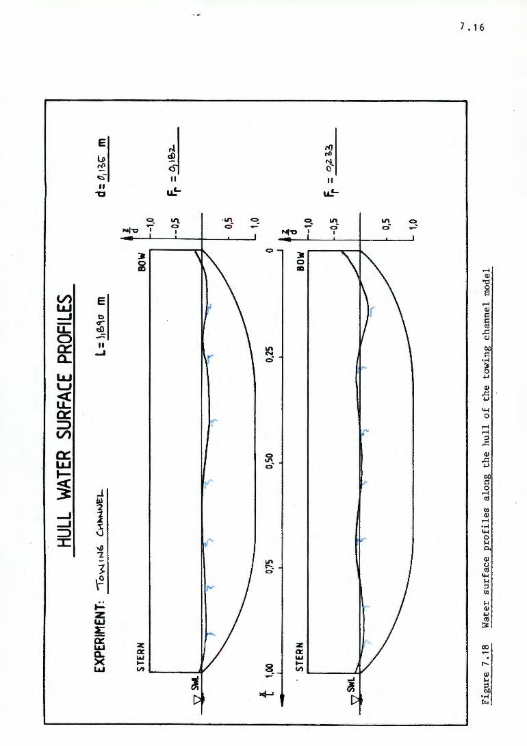
Univers
ity of
Cap
e Tow
n
HULL
W
ATER
SU
RFAC
E PR
OFIL
ES
EXPE
RIM
ENT:
-r
ow
1 N'-
C.~M
-1tJ
EL-
L:
\,e,
~o
m
STER
N BO
W
~
t 1,
00
0,75
0,50
0,
25
0
. ST
ERN
BOW
Fig
ure
7.1
8
Wat
er su
rface p
rofi
les
alo
ng
th
e h
ull
of
the
tow
ing
ch
ann
el m
odel
d:
tJ, 1
;{;
m
z d -1,0
-o.s
Fr =
o, 1e,
z.
0,5
·i
d
1,0
-u
-0,5
~ =
0z~a
0,5
1,0
"" "'
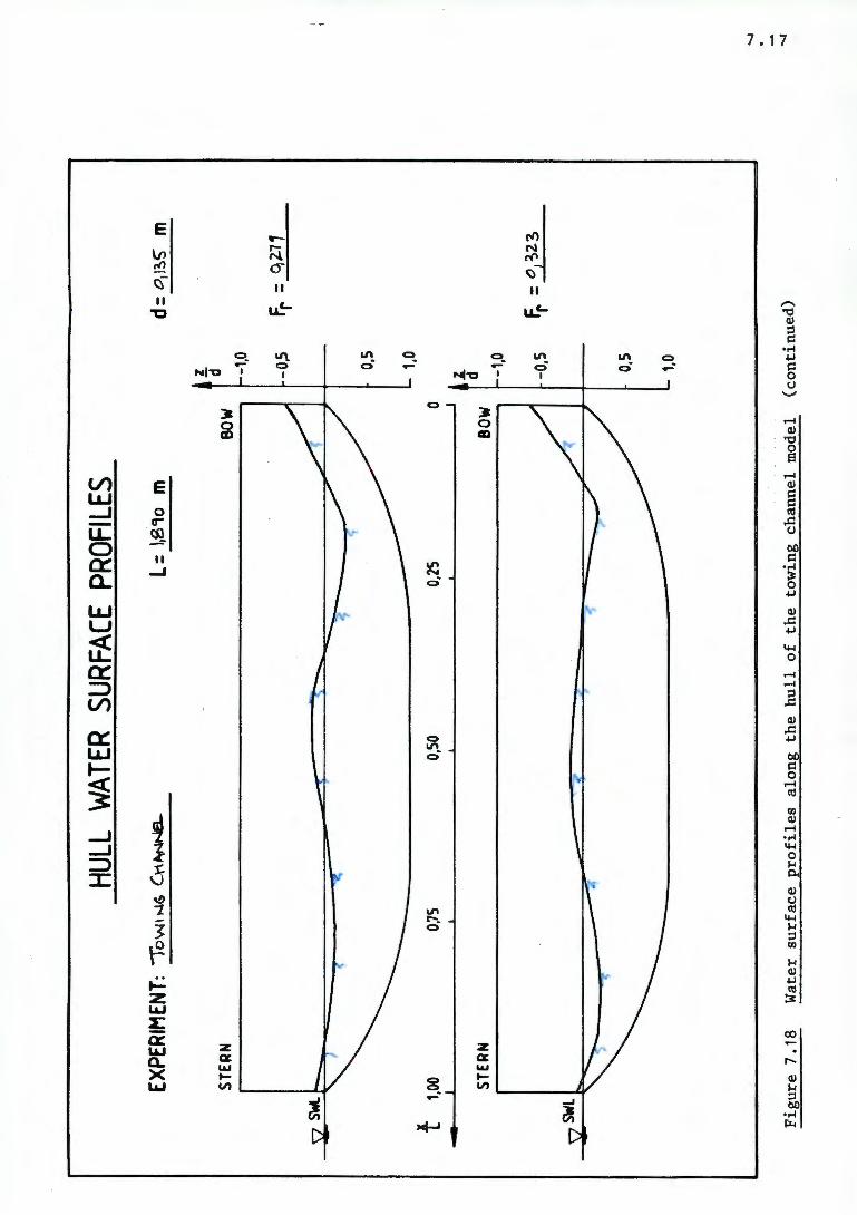
Univers
ity of
Cap
e Tow
n
HULL
W
ATER
SU
RFAC
E PR
OFI
LES
EXPE
RIM
ENT:
lo
w1
l'-lG
C.'"'~
L= l
,S9o
m
d=
o,1~s
m
z ST
ERN
BOW
Id
-1,0
-0,5
Fr
= o
,i..11
0,5
t 1,0
0 0,7
5 0,
50
0,25
0
1,0
.l
STER
N BO
W
Id -1,0
-0,5
Fr
= 0 1~2
3
0,5
1,0
"""'
Fig
ure
7.1
8 W
ater
su
rfac
e p
rofi
les
alo
ng
th
e h
ull
of
the
tow
ing
chan
nel
mod
el
(co
nti
nu
ed)
"""'
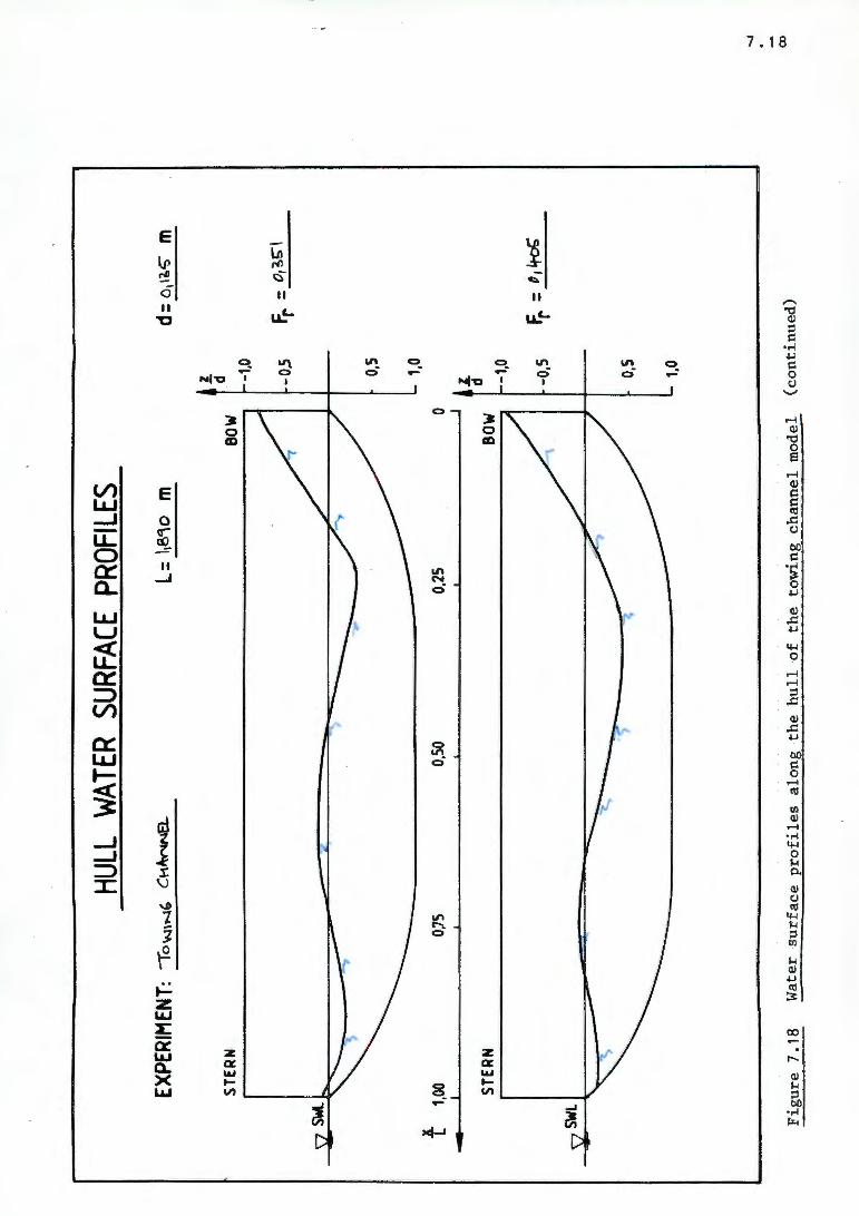
Univers
ity of
Cap
e Tow
n
HULL
W
ATER
SU
RFAC
E PR
OFIL
ES
EXPE
RIM
ENT:
-r
ow
1,.
.J(.
CH~El..
L= h
6C\o
m
d=
c11
it;"
m
z S
TER
N
BOW
d -1
.0
-o.s
Fr :
o, ;;
-1
0,5
1,0
t 1,
00
0,75
0,50
0,
25
0
l.
STE
RN
BO
W
Id -1,0
-0,5
Fr=~,~
0,5
1,0
........ ......
Fig
ure
7.1
8
Wat
er
surf
ace
pro
file
s al
on
g th
e h
ull
o
f th
e to
win
g
chan
nel
mod
el
(co
nti
nu
ed)
co
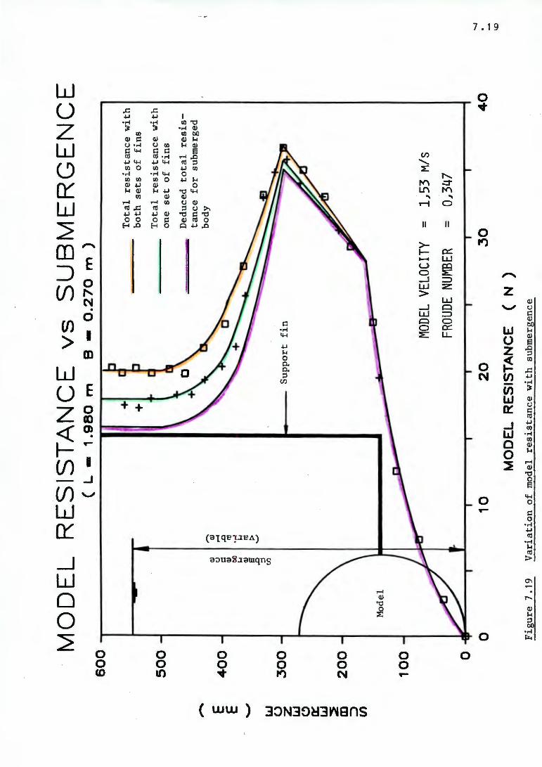
Univers
ity of
Cap
e Tow
n ""
E
E
.....
.., w
0 z w
C>
a:::
w
::?
m
:::>
(Jl
MO
DE
L
RE
SIS
TA
NC
E
vs
S
UB
ME
RG
EN
CE
(
L
-1
.98
0 m
8
-0
.27
0 m
)
60
0
.
50
0
40
0
30
0
20
0
10
0
0
-(I
) (I
) C
) ...
-I ~
,.0
(I
) rd
bO
•P
ol !-I
!-I
(I
) rd
s
:> ,.
0 ~
::l
U,)
0 1
0
To
tal
resi
stan
ce w
ith
b
oth
sets
o
f fi
ns
To
tal
resi
stan
ce w
ith
o
ne
set
of
fin
s
Ded
uced
to
tal
resis
ta
nce fo
r su
bmer
ged
body
Su
pp
ort
fin
~
20
MODE
L VE
LOCI
TY
=
1J53
Mis
FROU
DE N
UMBE
R =
OJ
347
30
MO
DE
L R
ES
IST
AN
CE
(
N
)
40
Fig
ure
7.1
9
Vari
ati
on
of
mod
el
resi
stan
ce w
ith
su
bm
erg
ence
"""
\0
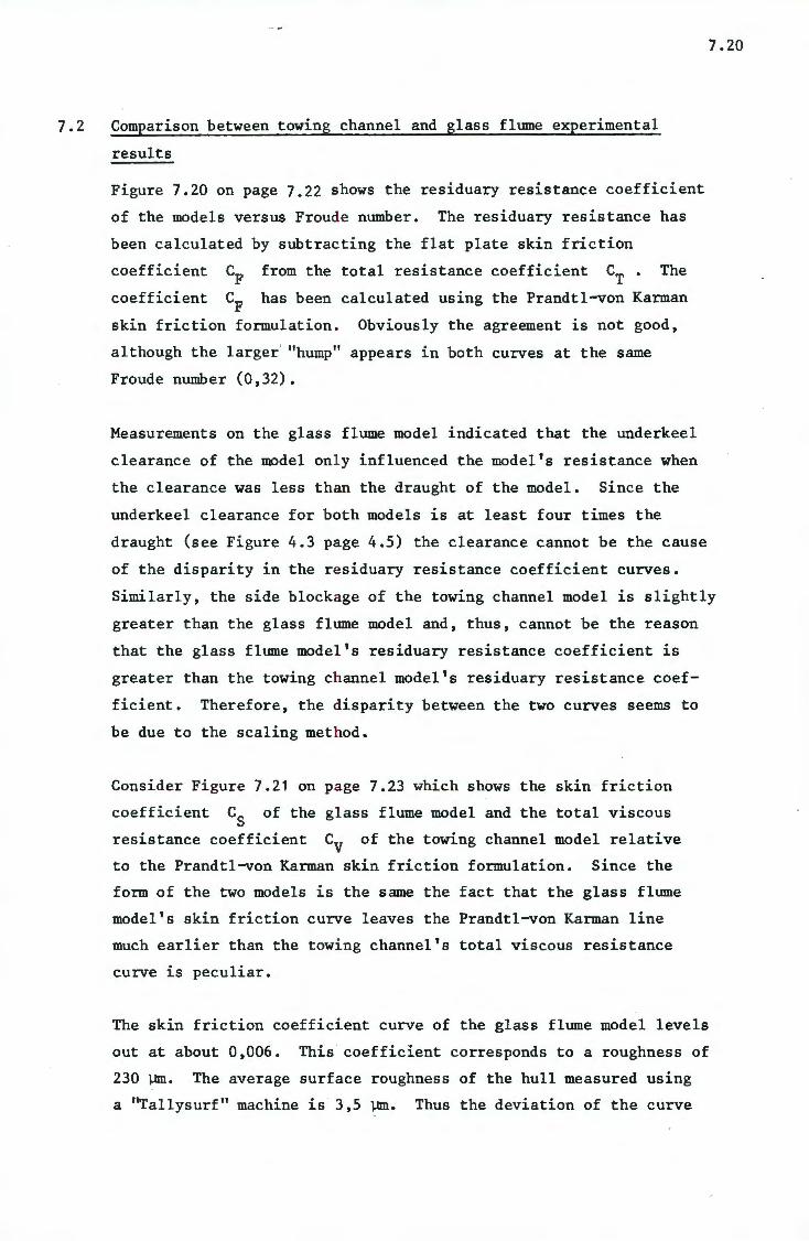
Univers
ity of
Cap
e Tow
n
7.2 Comparison between towing channel and glass flume experimental
results
Figure 7.20 on page 7.22 shows the residuary resistance coefficient
of the models versus Froude number. The residuary resistance has
been calculated by subtrac ting the flat plate skin friction
coefficient CF from the total resistance coefficient CT • The
coefficient CF has been calculated using the Prandtl-von Karman
skin friction formulation . Obviously the agreement is not good,
although the larger ' "hump" appears in both curves at the same
Froude number (0,32).
7.20
Measurements on the glass flume model indicated that the underkeel
clearance of the model onl y influenced the model's resistance when
the clearance was less than the draught of the model. Since the
underkeel clearance for both models is at least four times the
draught (see Figure 4.3 pa ge 4.5) the clearance cannot be the cause
of the disparity in the r esiduary resistance coefficient curves.
Similarly, the side blockage of the towing channel model is slightly
greater than the glass flume model and, thus, cannot be the reason
that the glass flume mode l 's residuary resistance coefficient is
greater than the towing channel model's residuary resistance coef
ficient. Therefore, the disparity between the two curves seems to
be due to the scaling method.
Consider Figure 7.21 on page 7.23 which shows the skin friction
coefficient CS of the glass flume model and the total viscous
resistance coefficient CV of the towing channel model relative
to the Prandtl-von Karman skin friction formulation. Since the
form of the two models is the same the fact that the glass flume
model's skin friction curve leaves the Prandtl-von Karman line
much earlier than the towing channel's total viscous resistance
curve is peculiar.
The skin friction coefficient curve of the glass flume model levels
out at about 0,006. This coefficient corresponds to a roughness of
230 µm. The average surface roughness of the hull measured using
a "Tallysurf" machine is 3,5 µm. Thus the deviation of the curve
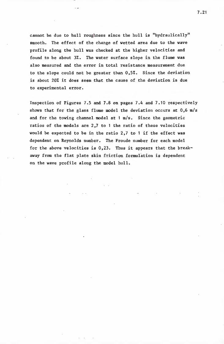
Univers
ity of
Cap
e Tow
n
cannot be due to hull roughness since the hull is "hydraulically"
smooth. The effect of the change of wetted area due to the wave
profile along the hull was checked at the higher velocities and
found to be about 3%. The water surface slope in the flume was
also measured and the error in total resistance measurement due
to the slope could not be greater than 0,5%. Since the deviation
is about 20% it does seem that the cause of the deviation is due
to experimental error.
Inspection of Figures 7.5 and 7.8 on pages 7.4 and 7.10 respectively
shows that for the glass flume model the deviation occurs at 0,6 m/s
and for the towing channel model at 1 m/s. Since the geometric
ratios of the models are 2,7 to 1 the ratio of these velocities
would be expected to be i n the ratio 2,7 to 1 if the effect was
dependent on Reynolds number. The Froude number for each model
for the above velocities is 0,23. Thus it appears that the break
away from the flat plate skin friction formulation is dependent
on the wave profile along the model hull.
7.21
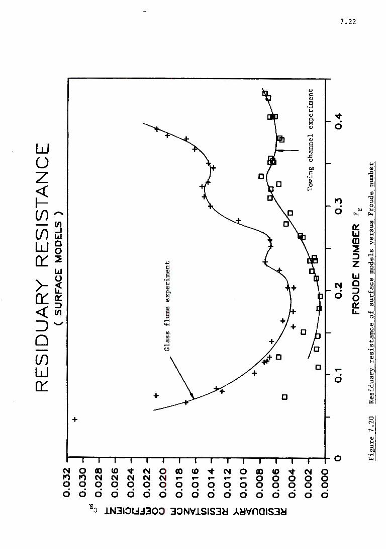
Univers
ity of
Cap
e Tow
n
RE
SID
UA
RY
R
ES
IST
AN
CE
(
SU
RF
AC
E M
OD
EL
S
)
Gla
ss
flu
me
exp
erim
ent
Tow
ing
chan
nel
ex
per
imen
t a
0.1
0
.2
0.3
0
.4
FR
OU
DE
NU
MB
ER
F
r
Fig
ure
7
.20
R
esid
uar
y re
sist
an
ce o
f su
rface m
od
els
ver
sus
Fro
ud
e nt
nnbe
r
""' . N
N
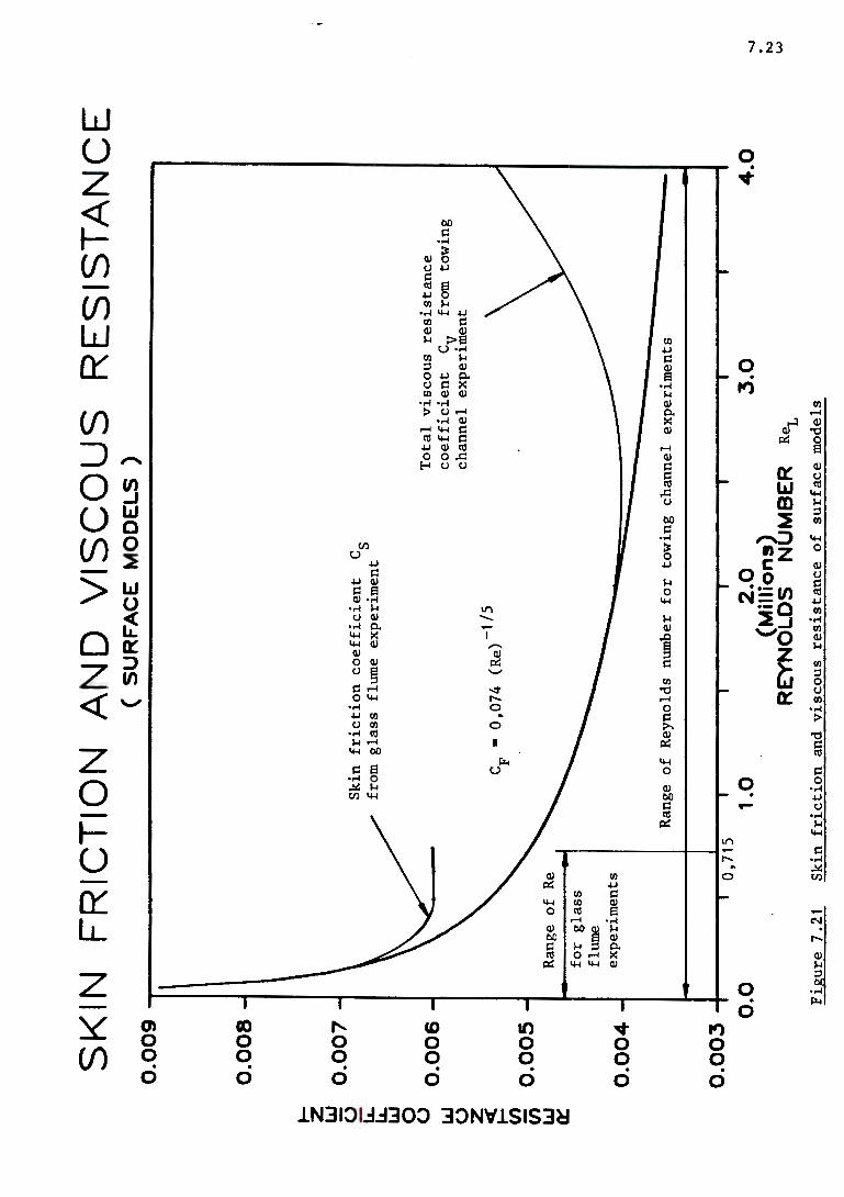
Univers
ity of
Cap
e Tow
n
~ z UJ - u u..
u..
UJ
0 u UJ
u z ~
(/)
(/)
UJ
0::
SK
IN
0.0
09
0.0
08
0.0
07
I 0
.00
6
I 0
.00
5
I ..
0.0
04
I
0.0
03
0.0
FR
ICT
ION
A
ND
V
ISC
OU
S
RE
SIS
TA
NC
E
\
' R
ange
o
f R
e
for
gla
ss
flum
e ex
per
imen
ts 0,7
15
/
( S
UR
FA
CE
MO
DE
LS
)
Sk
in fr
icti
on
co
eff
icie
nt
from
g
lass
fl
um
e ex
per
imen
t
CF
= 0
,07
4
(Re)
-1/5
cs
To
tal
vis
co
us
resi
stan
ce
co
eff
icie
nt
CV
from
to
win
g
chan
nel
ex
per
imen
t
Ran
ge
of
Rey
no
lds
num
ber
for
tow
ing
ch
ann
el
exp
erim
ents
1.0
2
.0
3.0
(M
illi
on
s)
RE
YN
OL
DS
N
UM
BE
R R~
4.0
Fig
ure
7.2
1 S
kin
fri
cti
on
an
d v
isco
us
resi
stan
ce o
f su
rface m
odel
s
....... . .....,
w
Univers
ity of
Cap
e Tow
n
CHAPTER 8
CONCLUSIONS
The deduced skin friction of the glass flume model deviated from the
Prandtl-von Karman skin friction formulation for flat plates. This
is probably due to the fact that the local fluid speeds around the
hull are increased due to the form of the hull, resulting in a higher
skin friction than would be measured on a flat plate. In the experi
mental work this deviation was found to occur at Froude number of 0,23
for both the models, indicating that the onset of the deviation from
Prandtl-von Karman formulation is dependent on the wave-profile along
the model hull.
The measured total viscous resistance of the towing channel model shows
a marked increase in the viscous resistance coefficient at Reynolds
numbers greater than 3 x 10 6 • Thus the viscous pressure resistance
seems to be significant and should, therefore, be included in the
component of resistance that i s scaled using Reynolds number scaling.
To circumvent the joint problems of obtaining the skin friction and
viscous pressure resistance (i.e. the total viscous resistance) of a
model, the total viscous resis t ance of reflex model could be measured.
This would entail additional expense during model testing as two models
would have to be made, but the rewards of predicting the power require
ment of a ship more accurately should justify the additional cost.
8. 1
Univers
ity of
Cap
e Tow
n
BIBLIOGRAPHY
Allan, J.F., Conn, J.F.C., 1950
"Effect of laminar flow on ship models"
Royal Institution of Naval Archi tects, Vol 92
Batchelor, G.K., 1977
"An introduction to fluid dynamics"
Cambridge: Cambridge University Press
Betts, P.L., Binnie, A.M., 1966
"Some experiments on ship models held in a small open water-channel
with slotted walls"
Royal Institution of Naval Archi tects, Vol 108
Bellhous~, B.J., Shultz, D.L., 1966
''Determination of mean and dynamic skin friction, separation and
transition in low speed flow with a thin film heated element"
Journal of Fluid Mechanics, Vo l 24, part II
Blevins, R.D., 1984
"Applied fluid dynamics handbook"
New York: Van Nostrand Reinhol d
Cole, A.J., Millward, A., 1977
"The measurement of skin friction on a planning hull using a
miniature Preston tube"
Royal Instltution of Naval Architects, Vol 119
Comstock, J.P., 1980
"Principles of naval architecture"
New York: Society of Naval Ar chitects and Marine Engineers
BIB .1
Univers
ity of
Cap
e Tow
n
Daugherty, R.L., Franzini, J.B. , 1977
"Fluid mechanics with engineering applications", 7th edition
Tokyo: McGraw-Hill
Davies, P.O.A.L., Kimber, G.R., 1976
"Skin friction measurement with a heated film"
Sixth thermodynamics and fluid mechanics convention
London: Institution of Mechanical Engineering Conference Publications
Emrich, R.J., 1981
''Methods of experimental physics : fluid dynamics"
New York: Academic Press
Francis, J.R.D., 1975
"Fluid mechanics< for engineering students", 4th edition ' London: Edward Arnold
Froude, W., 1872
"Experiments on the surf ace fric tion experienced by a plane moving
through water"
British Association for the Advancement of Science
Froude, W., 1874
"On experiments with H.M.S. Greyhound"
Institution of Naval Architects, Vol 16
Froude, W., 1874
"Experiments for the determination of the frictional resistance
of water on a surface under various conditions"
British Association for the Advancement of Science
BIB.2
Univers
ity of
Cap
e Tow
n
Froude, W., 1874
"Experiments in relation to the pressure-log, with a description
of the apparatus employed"
British Association for the Advancement of Science
Froude, W., 1877
"Experiments upon the effect produced on the wave-making resistance
of ships by length of parallel midbody"
Institution of Naval Architects, Vol 19
Froude, R.E., 1881
"On the leading phenomena of the wave-making resistance of ships"
Institution of Naval Architects, Vol 23
Froude, R.E., 1888
"On the 'constant' system of notation of results of experiments on
models used at the Admiralty experiment works"
Institution :of Naval Architects, Vol 30
Gillmer, T.C., 1975
''Modern ship design", 2nd edition
Annapolis: Naval Institution Press
Goldstein, R.J., ·1983
°Fluid mechanics measurements"
New York: Hemisphere
Havelock, T.H., 1924
"Wave patterns and wave resistance"
Royal Institution of Naval Architects, Vol 66
BIB.3
Univers
ity of
Cap
e Tow
n
Head, M.R., Rechenberg, I., 1962
"The Preston tube as a means of measuring skin friction"
Journal of Fluid Mechanics, Vol 14, Part 1
Hughes, G., 1966
"An analysis of ship model resis tance into viscous and wave components"
Parts I and II
Royal Institution of Naval Architects, Vol 108
Hughes, G., 1967
'~An analysis of ship model resis tance into viscous and wave components"
Part III
Royal Institution of Naval Architects, Vol 109
Hughes, W.F., Brighton, J.A., 1967
"Theory and problems of fluid dynamics"
New York: Schaum
Inui, T., 1962
"Wave-making resistance of ships '.'
Society of Naval Architects and Marine Engineers
Keith, H.D., 1957
"Simplified theory of ship waves"
American Journal of Physics, Vol 25
Kent, J.L., 1958
"Ships in rough water"
London: Thoman Nelson
BIB.4
Univers
ity of
Cap
e Tow
n
Kilner, F.A., 1983
"Boundary layers on plates"
CE 540 course notes, Department of Civil Engineering, U.C.T.
Kwang, J.B., McCarthy, J.H., 1979
"Ship wave-resistance computations"
Maryland: David Taylor Naval Ship Research and Development Centre
Lackenby, H., 1962
"Resistance of ships with specia l reference to skin friction and hull
surface condition"
Institution of Mechanical Engineers
Lackenby, H., 1965
"An investigation into the nature and interdependence of the components
of ship resistance"
Royal Institution of Naval Architects, Vol 107
Landweber, L., Patel, V.C., 1979
"Ship boundary layers"
Annual Review of Fluid Mechanics
Larson, L., 1977
"An experimental investigation of the three-dimensional turbulent
boundary layer on a ship model"
Institution of Mechanical Engineers
Manning, G.C., 1930
"Manual of Naval Architecture"
New York: Van Nostrand
BIB.5
Univers
ity of
Cap
e Tow
n
Matheson, N., Joubert, D.N., 1973
"Experimental determination of the components of resistance of a small
0,80 CB tanker model"
Journal of Ship Research, Vol 17
Matheson, N., Joubert, P.N., 1974
"A note on the resistance of bodies of revolution and ship forms"
Journal of Ship Research, Vol 18
McCarthy, J.H., Power, J.L., Huang, T.T., 1977
"The roles of transition, laminar separation and turbulence stimulation
in the analysis of axisyumetric body drag"
Institution of Mechanical Engineers
Millward, A., 1981
"The effect of shallow water of t he resistance of a ship at high
sub-critical and super-critical speeds"
Royal Institution of Naval Archit ects, Vol 12~
Millward, A., 1982
"Shallow water and channel effect s on ship wave resistance at high
sub-critical and super-critical speeds"
Royal Inst1tution of Naval Archi t ects, Vol 124
Miyata, H., Inui, T., 1984
"Non-linear ship waves"
Advances in Applied Mechanics, Vol 24
Muckle, W., 1975
"Naval Architecture for Marine Engineers"
London: Newnes-Butterworths
BIB.6
Univers
ity of
Cap
e Tow
n
Patel, V.C., 1965
"Calibration of the Preston tube and limitations on its use in pressure
gr ad ient s"
Journal of Fluid Mechanics, Vol 23, part I
Paterson, A.J.C., 1986
"The analysis of ship wave resistance using close range photogrammetry"
MSc Dissertation, U.C.T.
Pope, R.J., Bellhouse, B.J., 1971
BIB.7
"Measurement of local skin friction on ship models using thin film probes"
Royal Institution of Naval Archit ects, Vol 113
Potter, C.P., Foss, J.F., 1975
"Fluid Mechanics"
New York: .John Wiley
Preston, J.B., 1958
"The minimum Reynolds number fo r a turbulent boundary layer and the
selection of a transition device"
Journal of Fluid Mechanics, Vol 3, Part IV
Rahl, S.S., 1942
"Practical principles of naval architecture"
New York: Cornell Maritime Pres s
Rosenhead, L., 1963
"Laminar boundary layers"
Oxford: Clarendon Press
Univers
ity of
Cap
e Tow
n
/
Rossel, H.E., Chapman, L.B., 194 1
"Principles of Naval Architecture"
New York: Society of Naval Arch i tects and Marine Engineers
Saunders, H.E., 1972
"Hydrodynamics in ship design" Vol 1 and 2
New York: Society of Naval Archi tects and Marine Engineers
Schlichting, H., 1968
"Boundary layer theory" 7th edit i on
New York: McGraw-Hill
Shearer, J.R., Cross, J.J., 1~65
"The experimental determination of the components of ship resistance
for a mathematical model"
Royal Institution of Naval Architecture, Vol 107
Shearer, J.R., Steele, B.N., 1970
"Some aspects of the resistance of full form ships"
~oyal Institution of Naval Architecture, Vol 112
Sorensen, R.M., 1973
"Ship generated waves"
Advances in Hydroscience, Vol 9
Steele, B.N., Pearce, G.B., 1968
"Experimental determination of t he distribution of skin friction on a
model of a high speed liner"
Royal Institution of Naval Architecture, Vol 110
BIB.8
Univers
ity of
Cap
e Tow
n
Streeter, V.L., 1961
"Handbook of fluid dynamics"
New York: McGraw-Hill
Todd, F.H., 1966
"Viscous resistance of ships"
Advances in Hydroscience, Vol 3
Townsin, R.L., 1971
"The viscous drag of a 'Victory' model - results from wake and wave
pattern measurements"
Royal Institution of Naval Architects, Vol 113
Tulin, M.P., 1951
BIB.9
"The.separation of viscous drag and wave drag by means of the wake survey"
Washington: David Taylor Model Basin report 772
Vennard, J.K., Street, R.L., 1976
"Elementary fluid mechanics"
New York: John Wiley
Wehansen, J.V., 1973
"The wave resistance of ships"
Advances in Applied Mechanics, Vol 13
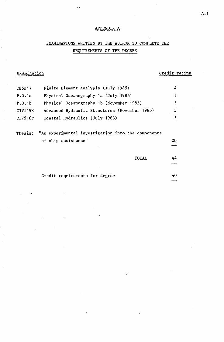
Univers
ity of
Cap
e Tow
n
APPENDIX A
EXAMINATIONS WRITTEN BY THE AUTHOR TO COMPLETE THE
REQUIREMENTS OF THE DEGREE
Examination Credit rating
CE~B-17
P.0.1a
P.0.1b
Finite Element Analysis (July 1985)
Physical Oceanography 1a (July 1985)
Physical Oceanography 1b (November 1985)
4
5
5
CIV519X Advanced Hydraulic Structures (November 1985) 5
CIV516F Coastal Hydraulics (July 1986)
Thesis: "An experimental.investigation into the components
of ship resistance"
TOTAL
Credit requirements for degree
5
20
44
40
A.1
Univers
ity of
Cap
e Tow
n
A.2
UNIVERSITY OF CAPE TOWN
DEPARTMENT OF CIVIL ENGINEERING
FINAL EXAM. MONDAY, 24 JUNE 1985
CE SB17 FINITE ELEMENT ANALYSIS
TIME 3 hours
Note:
The student may refer to class notes and assignments.
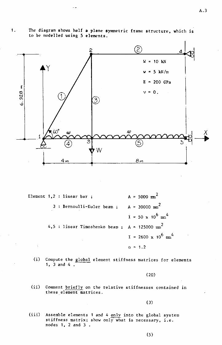
Univers
ity of
Cap
e Tow
n
1. The diagram shows half a plane symmetric frame structure, which is to be modelled using 5 elements.
2 ® w :: 10 kN
y w = 5 kN /rn
E = 200 GPa
\) c 0.
3
8 rr1
A 5000 2 = mm Element 1,2 linear bar ;
A 30000 mm 2 = 3 Bernoulli-Euler beam
I 6 4
= 50 x 10 mm
4,5 linear Timoshenko beam A 125000 mm 2
=
I 2600 x 106 4 = mm
a: = 1.2
(i) Compute the global element stiffness matrices for elements 1, 3 and 4 •
(20)
(ii) Comment briefly on the relative stiffnesses contained in these element matrices.
(iii)
(3)
Assemble elements 1 and 4 onlv into the global system stiffness matrix; show only---what is necessary, i.e. nodes 1, 2 and 3 .
(5)
A.3
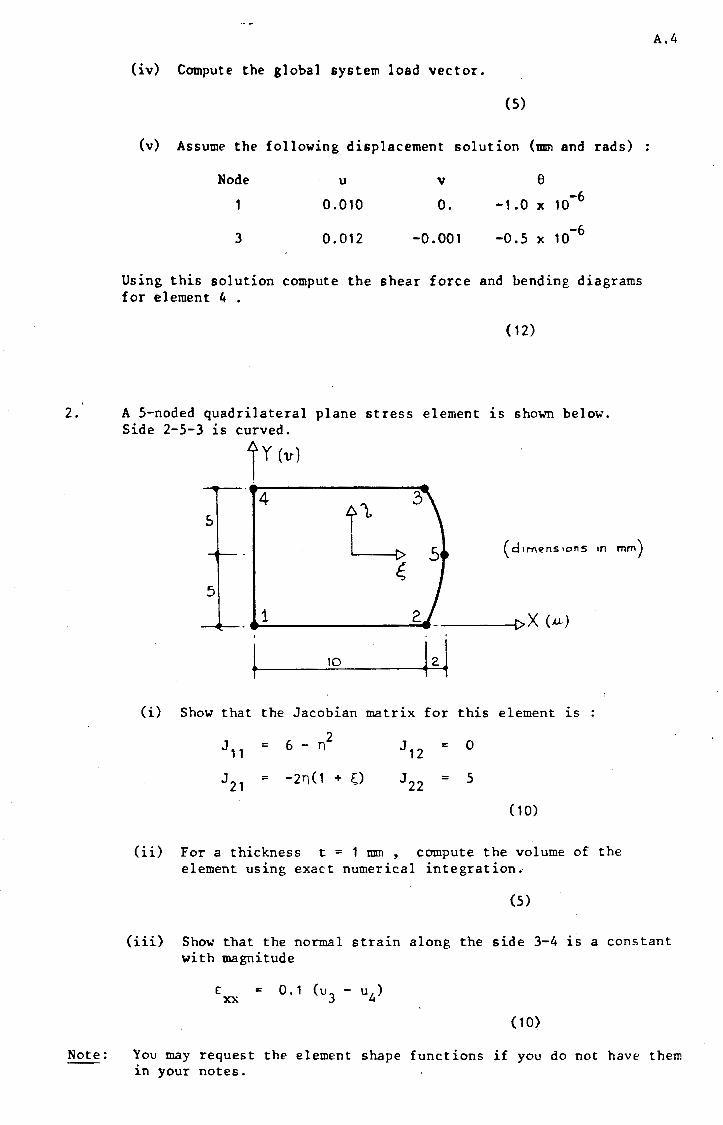
Univers
ity of
Cap
e Tow
n
(iv) Compute the global system load vector.
(5)
(v) Assume the following displacement solution Ctmn and rads)
Node u v e 1 0.010 o. -1.0 x 10⁻⁶
3 0.012 -0.001 -0.5 x 10⁻⁶
Using this solution compute the shear force and bending diagrams for element 4 .
( 12)
A.4
2. A 5-noded quadrilateral plane stress element is shown below.
Note:
Side 2-5-3 is curved. i y (tr)
(d1rnens1ons in mm)
4
L 3
~ 5
1 2- ---t>X (.u) . .
10 ~2l (i) Show that the Jacobian matrix for this element 15
J11 6 - n 2
J12 0 = =
J21 = -211 ( 1 + 0 J22 = 5
( 10)
(ii) For a thickness t = 1 mm ' compute the volume of the
element using exact numerical integration.
(5)
(iii) Show that the normal strain along the side 3-4 is a constant with magnitude
( 10)
You may request the element shape functions if you do not have them in your notes.

Univers
ity of
Cap
e Tow
n
3. A parabolic shear load is applied across the edges of two 8-node quadrilateral elements as shown in the diagram.
5
h 4
A.5
3P [ 2 2J pc:--h -y
3 4h3
h 2
1
Show that the equivalent nodal load at node 3 is (11/40)P
( 15)
4. A 4-node quadrilateral element and a 2-node bar element together support a point load P = 6000N • Nodes 1, 3 and 4 are fully restrained, and node 2 can only move horizontally.
3 1 mm
80rnm A =- 100 mrn
2
The following additional information is given
()N 2 ()N2 1
= -(1-n) - -(1+F) dX 16 ay 12
~ -[: :] E = 300 GPa \) = 0.3
Compute the horizontal displacement at node 2.
(15)
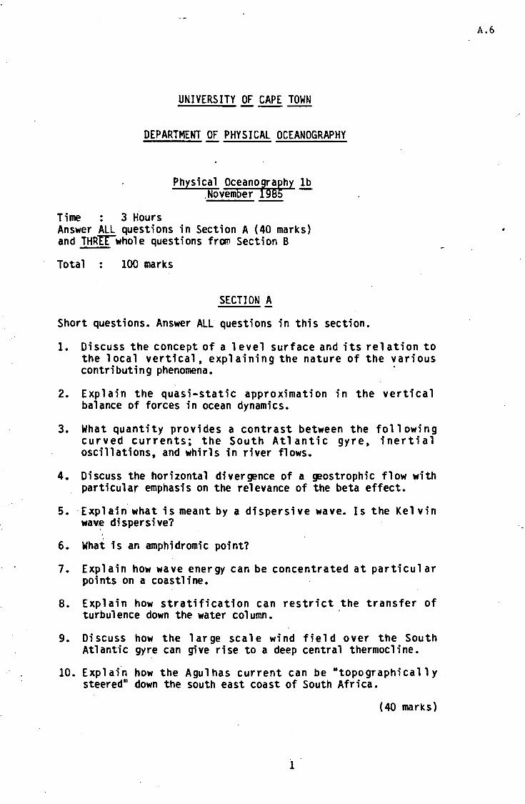
Univers
ity of
Cap
e Tow
n
UNIVERSITY OF CAPE TOWN
DEPARTMENT OF PHYSICAL OCEANOGRAPHY
Time 3 Hours
Physical Oceano~aphy lb .November 85 -
Answer ALL questions in Section A (40 marks) and THRrr-whole questions fraT1 Section B
Total . . 100 marks
SECTION A
Short questions. Answer ALL questions in this section.
1. Discuss the concept of a 1eve1 surf ace and its relation to the local vertical, explaining the nature of the various contributing phenomena. ·
2. Exp 1 ai n the quasi .. static approximation in the verti ca 1 balance of forces in ocean dynamics.
3. What quantity provides a contrast between the following curved currents; the South Atlantic gyre, inertial oscillations, and whirls in river flows.
4. Discuss the horizontal divergence of a geostrophic flow with particular emphasis on the relevance of the beta effect.
5. Explain what is meant by a dispersive wave. Is the Kelvin wav.~ dispersive?
6. What is an amphidromic point?
7. Explain how wave energy can be concentrated at particular points on a coastline.
8. Explain how stratification can restrict the transfer of turbulence down the water column. ·
9. Discuss how the 1 ar ge sea 1 e wind fie 1 d over the South Atlantic gyre can give rise to a deep central thermocl ine.
10. Explai~ how the Agulhas current can be utopographically steered" down the south east coast of South Africa.
(40 marks)
1
A.6
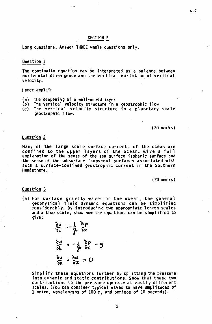
Univers
ity of
Cap
e Tow
n
SECTION B
Long questions. Answer THREE whole questions only.
Question l
The continuity equation can be interpreted as a balance between horizontal divergence and the vertical variation of vertical velocity. ·
Hence explain
(a) The deepening of a well-mixed layer (b) The vertical velocity structure in a geostrophic flow (c) The vertical velocity structure in a planetary scale
geostrophic fl ow.
(20 marks)
Question 1_
Many of 'the 1 ar ge sea 1 e surf ace cur rents of the ocean are confined to the upper layers of the ocean. Give a full explanation of the sense of the sea surface isobaric surface and the sense of the subsurface isopycnal surfaces associated with such a surface-confined geostrophic current in the Southern Hemisphere. .
(20 marks)
Question ~
(a) For surface gravity waves on the ocean, the general geophysical fluid dynamic equations can be simplified considerably. By introducing two appropriate length scales and a time scale, show how the equations can be simplified to give:
~ .. ' ~\O - s-f ~)( 'lt
'bw -l ~p -5 - -~l;. - !o b'%
~\.\ +~ ':: 0 -'b~ 't"%.
Simplify these ~quations further by splitting the pressure into dynamic and static contributions. Show that these two contributions to the pressure operate at vastly different scales. (You can consider typical waves to have amplitudes of 1 metre, wavel en_gths of 100 m, and periods of 10 seconds).
2
A. 7
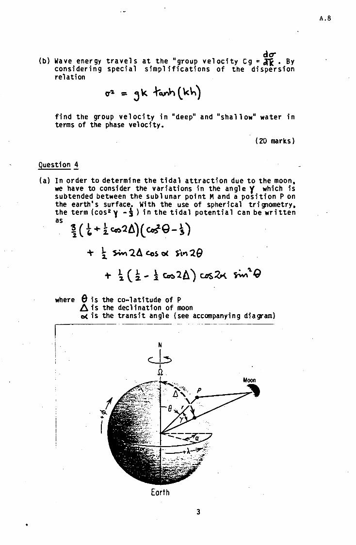
Univers
ity of
Cap
e Tow
n
•
dcr (b) Wave energy travels at the "group velocity Cg= Ji. By
considering special simplifications of the dispersion relation
find the group velocity in "deep" and "shallow" water in terms of the phase velocity.
(20 marks)
Question _i
(a) In order to determine the tidal attraction due to the moon, we have to consider the variations in the angle y which is subtended between the sub 1 unar point M and a position P on the earth's surface. With the use of spherical tri gnometry, the term (cos 2 'Y -i) in the tidal potential can be written as
i ( t + i ~'2!1)( cof9-j)
+ i SW\ '2.d Cos 0( s·l., 2 e + i(i-1~2/l)c.os~ ~"'Q
where e is the co-latitude of p l:l is the declination of moon o< is the transit angle (see accompanying diagram)
------. -------- .. -· ---- ------
·I ! !
N
c_b I .n.
Earth
3
A.8
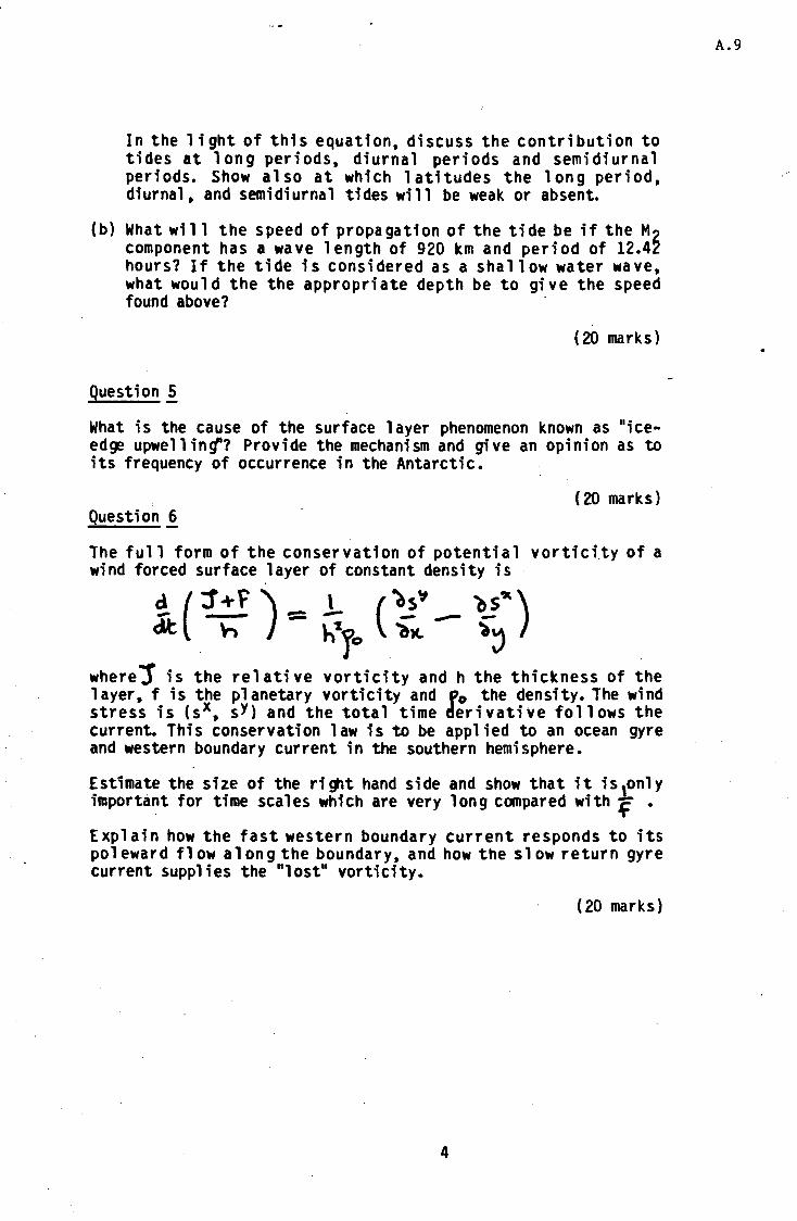
Univers
ity of
Cap
e Tow
n
(b)
In the light of this equation, discuss the contribution to tides at long periods, diurnal periods and semidiurnal periods. Show also at which latitudes the long period, diurnal, and semidiurnal tides will be weak or absent.
What wil 1 the speed of propagation of the tide be if the M2 component has a wave length of 920 km and period of 12.42 hours? If the tide is considered as a shallow water wave, what would the the appropriate depth be to give the speed found above? ·
( 20 marks)
Question~
What is the cause of the surface 1 ayer phenomenon known as 11 i ceed~ upwelling'? Provide the mechanism and give an opinion as to its frequency of occurrence in the Antarctic.
( 20 marks) Question!
The full form of the conservation of potential vortici.ty of a wind forced surface layer of constant density is
~ ( :r +f '= ..L (~" -- "b_!") dt . h J h)'o "llK. 'ii~
where'j' is the relative vorticity and h the thickness of the 1 ayer, f is the planetary vorticity and Po the density. The wind stress is (sx, sY) and the total time derivative follows the current. This conservation 1 aw is to be applied to an ocean gyre and western boundary current in the southern hemisphere.
Est1mate the size of the ri!jlt hand side and show that it is~nly important for time scales which are very long compared with f .
Explain how the fast western boundary current responds to its po 1 eward fl ow a 1 on g the boundary, and how the s 1 ow return gyre current supplies the "lost11 vorticity.
(20 marks)
4
A.9
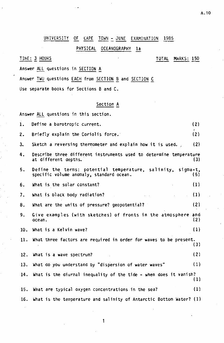
Univers
ity of
Cap
e Tow
n
UNIVERSITY OF CAPE TOWN - JUNE EXAMINATION 1985 - -- -----PHYSICAL OCEANOGRAPHY la
Tlt<1E: 3 HOU~S TOTAL MARKS: 150
Answer ALL questions in SECTION A
Answer TWU questions EACH from SECTION B and SECTION C
Use separate books for Sections B and C.
Section A
Answer ALL questions in this section.
1. Define a barotropic current. (2)
2. Briefly explain the Coriolis force. (2)
3. Sketch a reversing thermometer and explain how it is used. ) (2)
4. Describe three different instruments used to determine temperature at aifferent depths.· ( 3)
5. Define the terms: potential temperature, salinity, specific volume anomaly, standard ocean.
6. What is the solar constant?
7. What is black body radiation?
8. What are the units of pressure? geopotential?
sigma-t, ( 5)
( 1}
(1)
(2)
9. Give examples (with sketches) of fronts in the atmosphere and ocean. (2)
10. What is a Kelvin wave? ( 1)
11. What three factors are required in order for waves to be present.
12. What is a wave spectrum?
13. What Clo you understanel by "disp.ersion of water waves"
( 3)
( 2)
(1)
14. What is the Cliurnal inequality of tDe tide - when does it vanish? ( 1)
15. What are typical oxygen concentrations in the sea? ( 1)
16. what is the temperature and salinity of Antarctic Bottom Water? (1)
1
A.10

Univers
ity of
Cap
e Tow
n
Section B
Answer TWO questions ONLY from this section.
(i) Describe briefly, with sketches where necessary, the surface wind sys terns a round southern Africa. Distinguish between winter and summer circulation patterns and draw surface pressure maps typical of winter and summer. (30)
(ii) Describe briefly the major surface currents around southern Africa. Draw a map of the surface currents and indicate the major topographic features in relation to the currents. (30)
(iii) Given that there is no global gain or loss of heat in the ocean, write down the heat balance equation for the ocean. Describe the various terms and give the magnitude. Pay particular attention to the oetail of how the solar radiation reaches the sea surface.
( 30)
(iv) Describe the circulation and water masses in a section from pole to pole through the Atlantic ocean. Describe the circulation in a vertical section from pole to pole through the atmosphere. What is the jet stream and where can it be found? ( 30)
2
A. 11
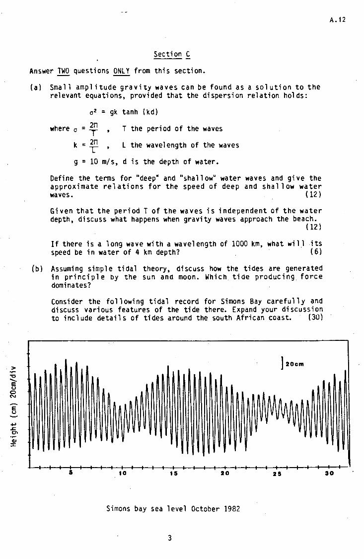
Univers
ity of
Cap
e Tow
n
> ..... "'O ....... e u 0 N -e u
..,
.r:. O'> ..... (1J ::c
Section C
Answer TWO questions ONLY from this section.
(a} Smal 1 amplitude gravity waves can be found as a solution to the relevant equations, provided that the dispersion relation holds:
02 = gk tanh (kd)
where a - 2n T the period of the waves - T ,
k = ~ , l the wavelength of the waves
g = 10 m/s, d is the depth of water.
Define the terms for "deep" and "shal 1 ow" water waves and give the approximate relations for the speed of deep and shallow water waves. (12)
Given that the period T of the waves is independent of the water depth, discuss what happens when gravity waves approach the beach.
( 12)
If there is a long wave with a wavelength of 1000 km, ~hat wilJ its speed be in water of 4 km depth? (6)
(b) Assuming simple tidal theory, discuss how the tides are generated in principle by the sun ana moon. Which tiae producing force dominates?
. .
Consider the following tidal record for Simons Bay carefully and discuss various features of the tide there. Expand your discussion to include details of tides around the south African coast. (30)
] 20cm
~\~
. - . . . . . I 10 15 20 25
Simons bay sea level October 1982
3
A.12
. . 30
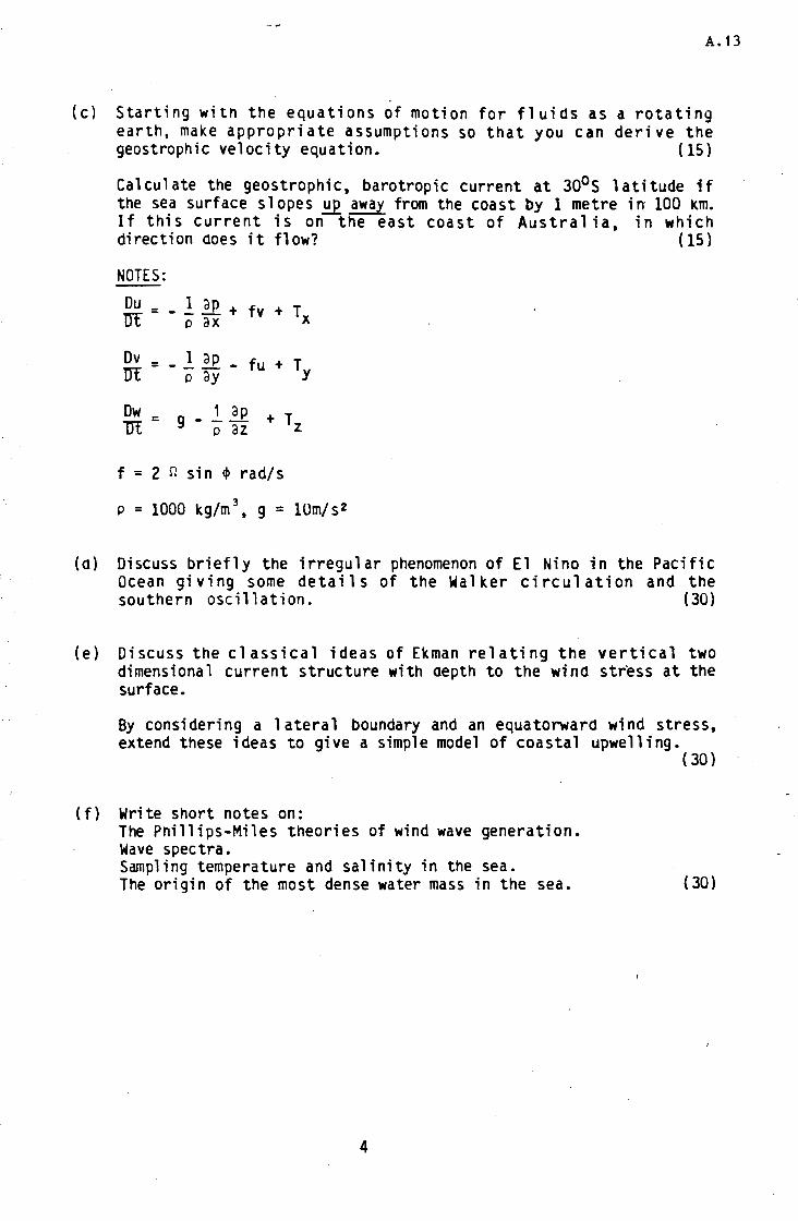
Univers
ity of
Cap
e Tow
n
A. 13
(c) Starting with the equations of motion for fluias as a rotating earth, make appropriate assumptions so that you can derive the geostrophic velocity equation. (15)
Calculate the geostrophic, barotropic current at 30°s latitude if the sea surf ace s 1 opes ~ away from the coast by 1 metre in 100 km. If this current is on the east coast of Australia, in which direction aoes it flow? (15)
NOTES:
Ou = 1 ap + f + T nt -'Pax v x
Ov = _ 1 ap _ fu + Ty nt 'Pay
Dw _ g _ .! ~ + T m - p az z
f = 2 n sin ~ rad/s
P = 1000 kg/m 3, g = 10m/s2
(a) Discuss briefly the irregular phenomenon of El Nino in the Pacific Ocean giving some details of the Walker circulation and the southern oscillation. (30)
{e) Discuss the classical ideas of Ekman relating the vertical two dimensional current structure with aepth to the wino stress at the surface.
By considering a l atera 1 boundary and an equatorwara wind stress, extend these ideas to give a simple model of coastal upwelling.
(f) Write short notes on: The Pnillips-Miles theories of wind wave generation. Wave spectra. Sampling temperature and salinity in the sea. The origin of the most dense water mass in the sea.
4
( 30)
( 30)
Univers
ity of
Cap
e Tow
n
UNIVERSITY OF CAPE TOWN
DEPARTMENT OF CIVIL ENGINEERING
COURSE CE SD5 : ADV.ARCED HYDRAULIC STRUCTURES
There is no written examination for this course.
The result will be assessed from two equal value projects.
Project 1
Project 2
Analysis of side channel spillway.
Analysis of side weir overflow.
September 1985.
A.14
Univers
ity of
Cap
e Tow
n
i.
URIVERSITY OF CAPE TOWN
DEPAR'l'MERT OF CIVIL EBGIREERIBG
M.Sc. in CIVIL EBGIREERIBG
URIVERSITY EXAMIBATIOB JULY 1986
CIV 516F : COASTAL HYDRAULICS
ALL questions may be attempted.
Constants
Sea water density = 1025 kg/m 3
Sea water height = 10 kN/m3
A. 15
( 4 PAGES )
Time: 4 hours
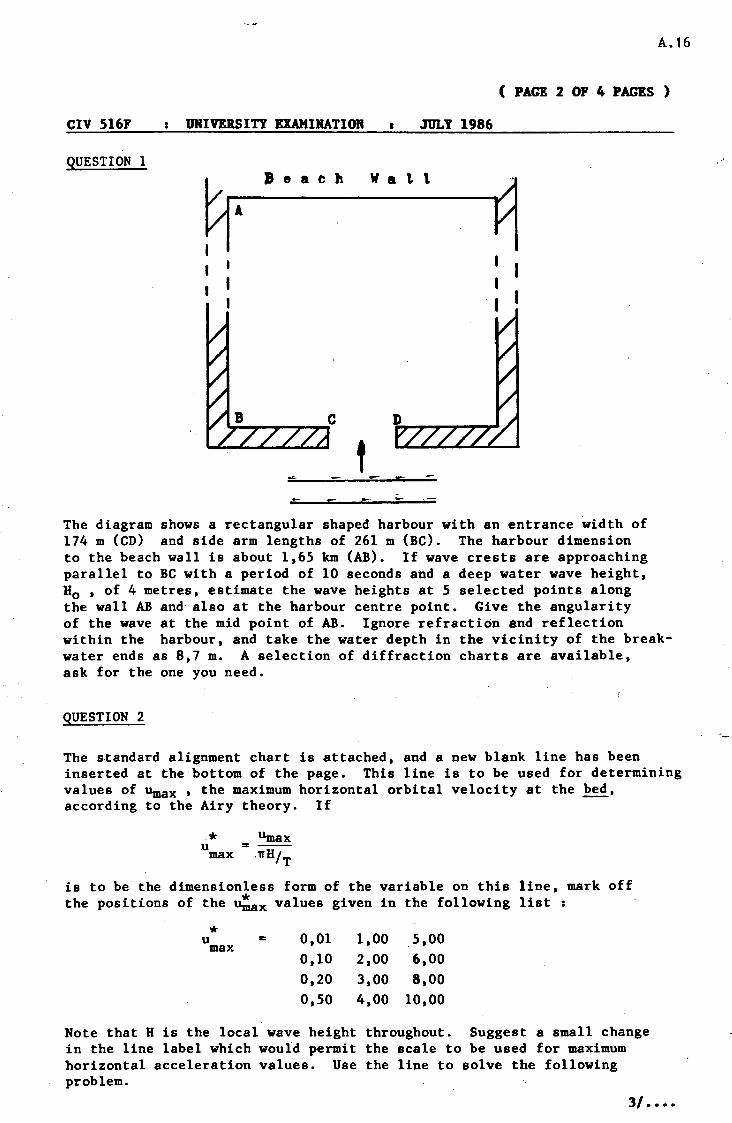
Univers
ity of
Cap
e Tow
n
A.16
( PAGE 2 OF 4 PAGES )
CIV 516F UlfIVERSITY EXAMIRATIOB I JULY 1986
QUESTION l Beach W a 1. t
' r
The diagram shows a rectangular shaped harbour with an entrance width of 174 m (CD) and side arm lengths of 261 m (BC). The harbour dimension to the beach wall is about 1,65 km (AB). If wave crests are approaching parallel to BC with a period of 10 seconds and a deep water wave height, H0 , of 4 metres, estimate the wave heights at 5 selected points along the wall AB and also at the harbour centre point. Give the angularity of the wave at the mid point of AB. Ignore refraction and reflection within the harbour, and take the water depth in the vicinity of the breakwater ends as 8,7 m. A selection of diffraction charts are available, ask for the one you need.
QUESTION 2
The s-tandard alignment chart is attached, and a new blank line has been inserted at the bottom of the page. This line is to be used for determining values of Umax , the maximum horizontal orbital velocity at the bed, according to the Airy theory. If
* u max
is to be the dimensionless form of the variable on this line, mark off the positions of the U:Sx values given in the following list :
* u max 0,01 0,10
1,00 2,00
5,00 6,00
0,20 3,00 8,00 0,50 4,00 10,00
Note that H is the local wave height throughout. Suggest a small change in the line label which would permit the scale to be used for maximum horizontal acceleration values. Use the line to solve the following problem.
3/ ••••
--
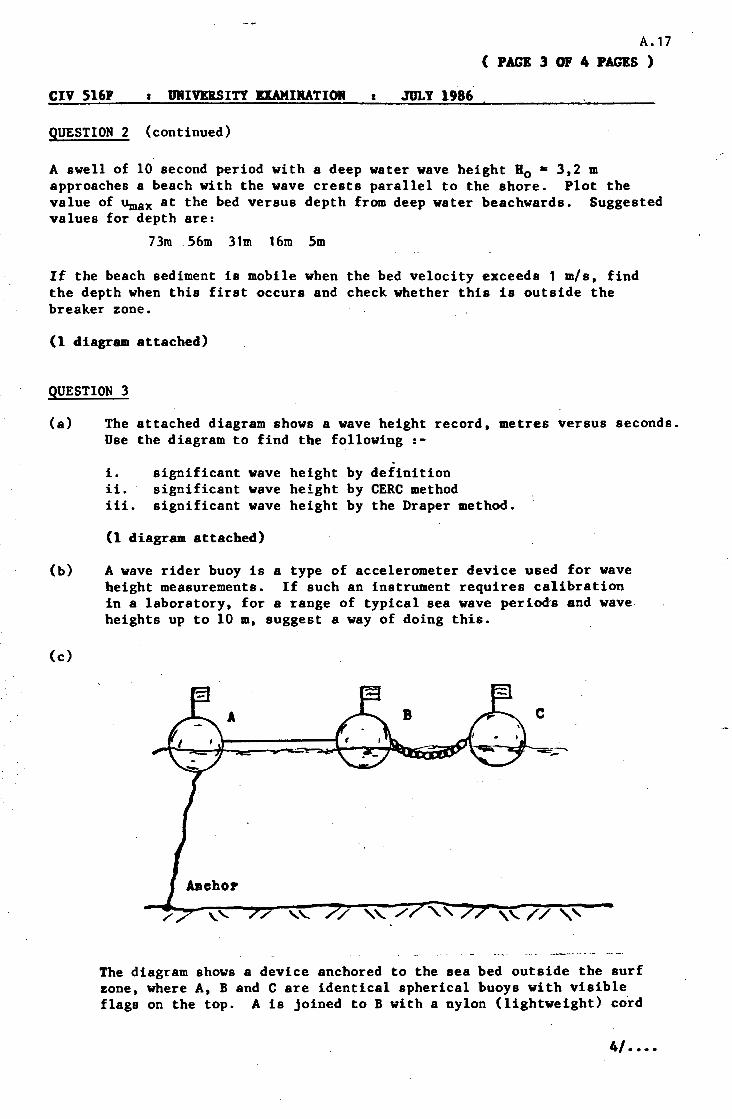
Univers
ity of
Cap
e Tow
n
CIV 516F URIVDSITY BIAMIRATIOll
QUESTION 2 (continued)
JULY 1986
A. 17 ( PAGE 3 OF 4 PAGES )
A swell of 10 second period with a deep water wave height H0 c 3,2 m approaches a beach with the wave crests parallel to the shore. Plot the value of Umax at the bed versus depth from deep water beachwards. Suggested values for depth are:
73ro 56m 31m 16m 5m
If the beach sediment is mobile when the bed velocity exceeds 1 m/s, find the depth when this first occurs and check whether this is outside the breaker zone.
(1 diagram attached)
QUESTION 3
(a) The attached diagram shows a wave height record, metres versus seconds. Use the diagram to find the following :-
. i. significant wave height by definition ii. significant wave height by CERC method iii. significant wave height by the Draper method.
(1 diagram attached)
(b) A wave rider buoy is a type of accelerometer device used for wave height measurements. If such an instrument requires calibration in a laboratory, for a range of typical sea wave perioas and wave heights up to 10 m, suggest a way of doing this.
(c)
/ ' '- '/ ,, / ,, // ,, The diagram shows a device anchored to the sea bed outside the surf zone, where A, B and C are identical spherical buoys with visible flags on the top. A is joined to B with a nylon (lightweight) cord
4/ ••••
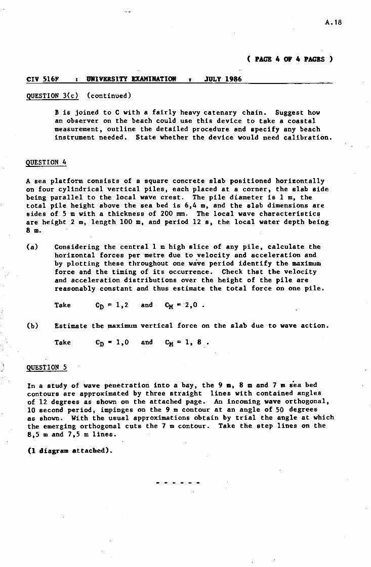
Univers
ity of
Cap
e Tow
n
• . -> '
A.18
( PAGE 4 OF 4 PAGES )
CIV 516F : URIVERSITY EXAMIRATIOR 1 .JULY 1986
QUESTION 3(c) (continued)
B is joined to C with a fairly heavy catenary chain. Suggest how an observer on the beach could use this device to take a coastal measurement, outline the detailed procedure and specify any beach instrument needed. State whether the device would need calibration.
QUESTION 4
A sea platform consists of a square concrete slab positioned horizontally on four cylindrical vertical piles, each placed at a corner, the slab side being parallel to the local wave crest. The pile diameter is 1 m, the total pile height above the sea bed is 6,4 m, and the slab dimensions are sides of 5 m with a thickness of 200 nun. The local wave characteristics are height 2 m, length 100 m, and period 12 s, the local water depth being 8 m.
(a) Considering the central 1 m high slice of any pile, calculate the horizontal forces per metre due to velocity and acceleration and by plotting these throughout one wave period identify the maximum force and the timing of its occurrence. Check that the velocity and acceleration distributions over the height of the pile are reasonably constant and thus estimate the total force on one pile.
Take Cn = 1,2 and
(b} Estimate the maximum vertical force on the slab due to wave action.
Take en = l,o and CM = 1, 8 •
\ . ' QUESTION 5
In a study of wave penetration into a bay, the 9 m, 8 m and 7 m sea bed contours are approximated by three strai_ght lines with contained angles of 12 degrees as shown on the attached page. An incoming wave orthogonal, 10 second period, impinges on the 9 m contour at an angle of 50 degrees as shown. With the usual approximations obtain by trial the angle at which the emerging orthogonal cuts the 7 m contour. Take the step lines on the 8,5 m and 7,5 m lines.
(1 diagram attached).
Univers
ity of
Cap
e Tow
n
B. 1
APPENDIX B
GLASS FLUME EXPERIMENT
B.1 Pressure tapping locations
B.2 Capillary rise in tubes
B.3 Calculation method for total pressure resistance
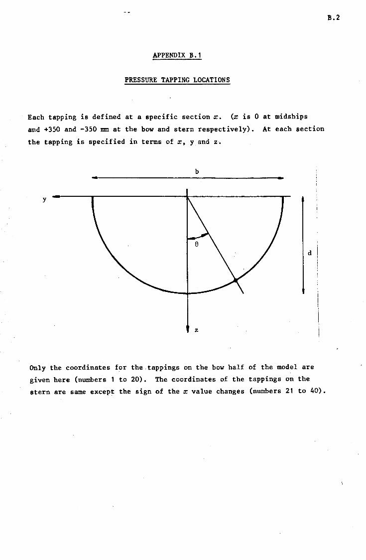
Univers
ity of
Cap
e Tow
n
APPEND IX B • 1
PRESSURE TAPPING LOCATIONS
Each tapping is defined at a specific section x. (x is 0 at midships
and +350 and -350 nm at the bow and stern respectively). At each section
the tapping is specified in terms of x, y and z.
b
y
d
z
Only the coordinates for the.tappings on the bow half of the model are
given here (numbers 1 to 20). The coordinates of the tappings on the
stern are same except the sign of the x value changes (numbers 21 to 40).
B.2
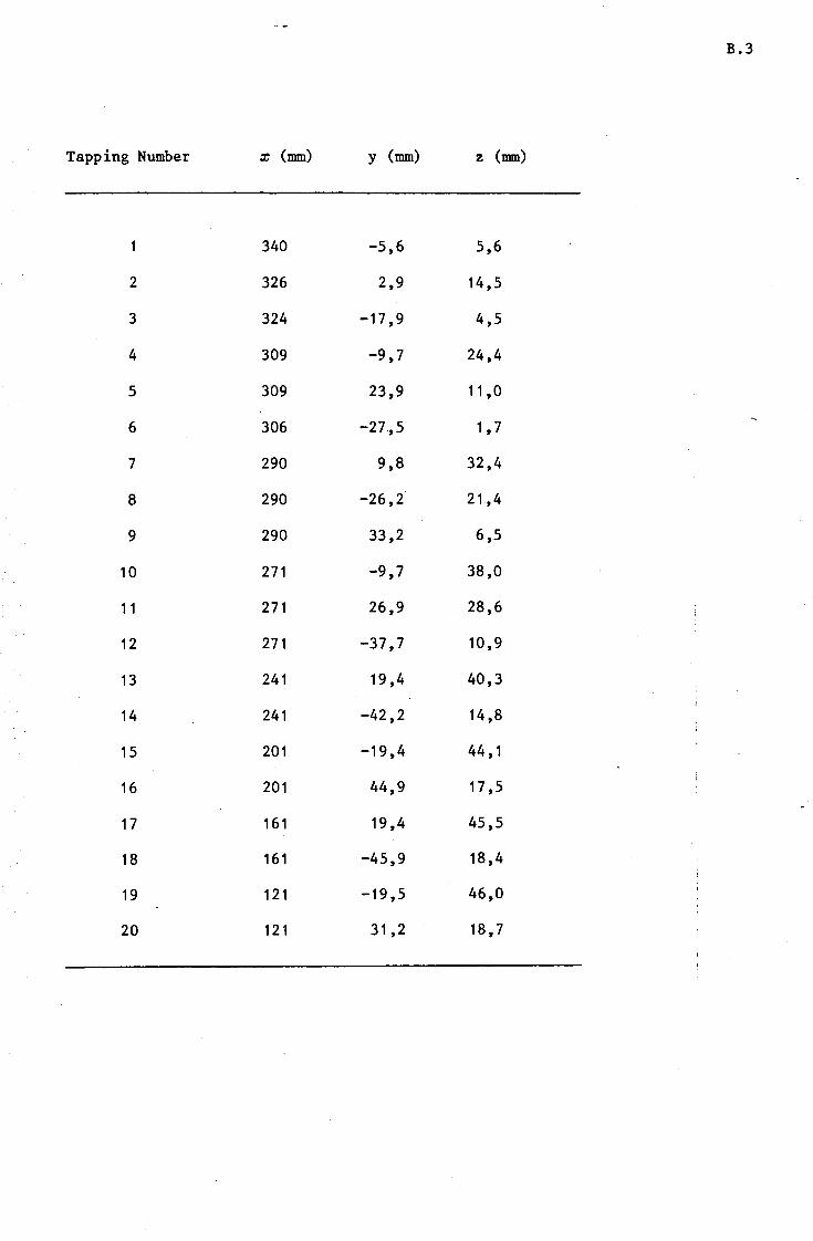
Univers
ity of
Cap
e Tow
n
B.3
Tapping Number x (mm) y (mm) z (mm)
340 -5,6 5,6
2 326 2,9 14,5
3 324 -17,9 4,5
4 309 -9,7 24,4
5 309 23,9 11,0
6 306 -27.,5 1 '7
7 290 9,8 32,4
8 290 -26,2 21,4
9 290 33,2 6,5
10 271 -9,7 38,0
11 271 26,9 . 28,6
12 271 -37,7 10,9
13 241 19,4 40,3
14 241 -42,2 14,8
15 201 -19,4 44, 1
16 201 44,9 17,5
17 161 19,4 45,5
18 161 -45,9 18,4
19 121 -19,5 46,0
20 121 31,2 18,7
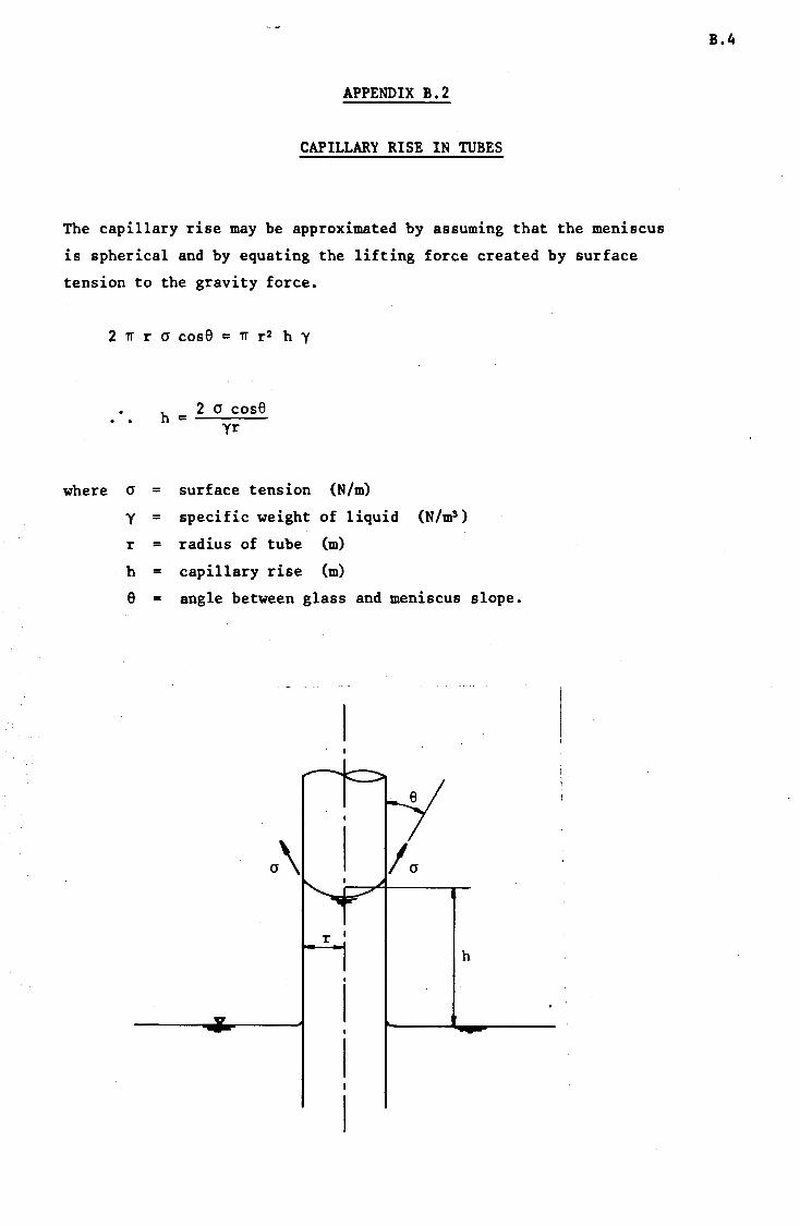
Univers
ity of
Cap
e Tow
n
APPENDIX B.2
CAPILLARY RISE IN TUBES
The capillary rise may be approximated by assuming that the meniscus
is spherical and by equating the lifting force created by surface
tension to the gravity force.
where
2 n r a cos8 = n r2 h y
a
y
r
h
h = 2 a cos8 yr
= surface tension
= specific weight
= radius of tube
= capillary rise
(N/m)
of liquid (N/m3 )
(m)
(m)
e = angle between glass and meniscus slope.
. I
r I
h
B.4
Univers
ity of
Cap
e Tow
n
a = 0,0728 N/m at 20°C
y = 9,81 x 10³ N/m3
r = 10 x 10-3 m
e = oo for a clean glass tube
h = 1,484 mm
This rise in the tube is relatively small. However, it will not affect
the pressure measurements since it will occur in all the glass tubes.
B.5
Univers
ity of
Cap
e Tow
n
B.6
APPENDIX B.3
CALCULATION METHOD FOR TOTAL PRESSURE -RESISTANCE
An example of the calculation method is shown on pages B.7 to B.12.
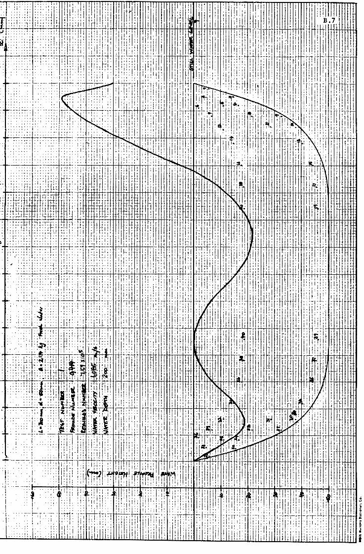
Univers
ity of
Cap
e Tow
n
I ..
' . . . .
.. 8 : "' ..
. , ... .... . ' .-....;...__..,..-++__..-.-.......,.+......++
··• .
.. :J' I
•••I.•
~-,-: ............. ~~~,-.-,..;-,-+....++. ,.
-~~1 · ,.
' I I I
·1.
·I· ' ··-·-·•-·
'' I
" i '. ! ' ..
• • fl . ' I'• ''' 11 f' ! '
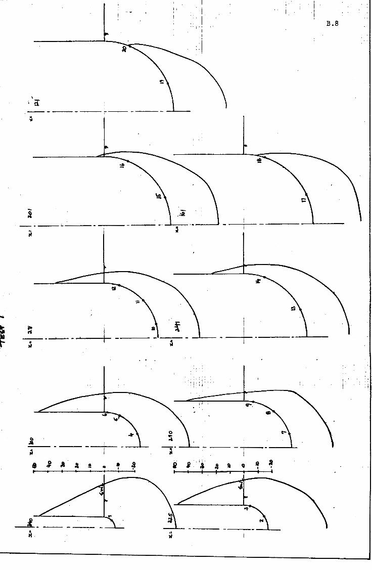
Univers
ity of
Cap
e Tow
n 'l -.9 .. J i -:)
~ .II
-)
~ 0
IXl
~
\
i !I --------------
-~
;... .. ~
:: __ ___,___
• ,,
a .. ;i
• : A !\ .!
-'----,.
.
...
• a ~ I
I , . I I; , I I 'i I I B.8 '' ''
I ! ' I
:: I
' . .:::!
' .• ~
~
'' '
: ! : : i:
!·• .... .
0
~
-~-
i I l A !l q 9 :i I .
,, w
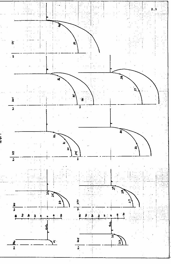
Univers
ity of
Cap
e Tow
n "l --0 F. ;i
, I::. .. ! :
i.
. , !
. ! I I
i : :: : I 1 ·-:: i.
------- --- r---- ----
-! ~
-------___ ___,~
Q .. ;s
" ' : ! --
i. . : ~I : l
I i· i
: . I . ~~·-. !
• ~. -----~-- --+--··--·-~
--- ----
. (:
. ! ! . i . 1 ·'" .. · 1 (:":
! ] '
.. : . : ~~ :..:.1 ... : I
I' . : j: !
I .
I.
~
:· J . ' : : j ... --~--~~. -:-r-
• 1 ! .
: I
0,
~: ' : · --- ---·-- ;_· ---~' . .:.
. '- .
i J? ; : ...... . A !l. Q
-~-··--r-t . -L ... . • .. . i.
i. I'
•• w
-·- •• L,.
a . I ' I
I : ., . .. , , ' . ' . ''
' ; . ~ ' "
. ' ~
. ; .
' ~ '
' ' .. • ';. !
. 'i
. i.
i '.
. I
l.' B.9
':: ! i ! . : 'I'.; ': r'. •
.. : . : i ~;
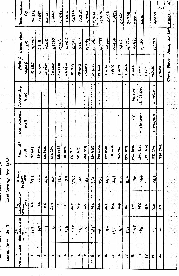
Univers
ity of
Cap
e Tow
n
~ -
j ' 1 ' I I ~ ..
'' .. '
. ··-B .10 '.
~ ·'-'> Jo. N . '
·.~ ~ - ~ tp' <D ~ IJI .o ~ N .rl '~..,.... ~ 0 ~ N - ~ •j ••·t-:-
N - ..,A ·\fl
~ V> ' . ' - '8 N 8 ~ 8 :~ - -.JI
! 0 5 0 C) () . (,) ~ 9. Q -cl ~ '<:S cS' . ....... . _ .. 0 <::! .. <5 t)' 0 () cS .~ .~ 0 C) - c) c5 . ()' 0 .. <::) ~ . .
'. '. I•. . . ·- .. ··-
~ .. . . .. c:i.: l '. ; : ..
',.' . ' . '' ·q:- 4 . r.- .rl
:~ V"- ' ..:t- ~~
r--- ..J) • N - \I) . - ··~ (Q" V> 0 ·;:I ""' ' V" t ~ -:t:- ~ '...,£) ~ t; ~ r- ~
' () lJl 0 ~ 0 ~ ..... r-1 ~ ~·
~ ..... - N
0 0 ~ - 0 <:;) .j-~ ~
\) r-
.cS' c$" ~ ·~ <S' <S' ~ Q '·- . G" ~ ~ ~ (,... ~ J . ti
. '.
~ .. . '
J. .. ' ''
~1 ..... ..... ·~ QC) a> 0
i ~ \'!' ... d) ,, ~ t :ii .t: .... .... .... ~ .... cO • ~ l l _ ... ... ,...
3 -· 'I) .. .... ~ ~ i :~ . l-; : .J - 111 ts § :;;;: ! :#. ... ' .. '.:t- () a ..... ii -' ;f s d) $ "' '° ·~. :~ ' .;, to ,...;. C'li ,.;, ~. ~
~·.·. . "' ~ - ~ .... ~. ~ ~ t· .. . ...
I . '.: '' '. '' . '' . '. I ~ .'..-.... -· --, 'I· . ' . ' , ,
11' . ' ~ J : ; 1 ! · 1 ••
·ts '1 •I
I .. ' ',,. . ; '
~ : '. '' '. ; ; : ; .. '. '. °' . .
' '. '! 1 . ! • '. ~ - v;- ... ll .. '. . .
. ........ , - .... - - -· -- _, ....... - ~ : : . ' er-''. , Ii·
:·~ (I"' . ' . ' ' .. jo-
. '. f. . . '.' . .;to: ; ·t- . . ~ . , . ..... I I• ... ' . '' , , , . '' . ' - r,-4 r4 .. . .... . ' ! ·I• I . ' . ' .... . . '' .. I I I' ! ': ! . ' • 'If' ' .. ' .. ' '' ··~ - --·
~ - ··- ·--· . . - '. ' . •It i . ' ~ .. '
J I .. ' -
~ . '
I '. . \n ~ ...
'' ''
I . . Q .... ' .
! """ '\A . - • • - ·-r --·- '. ' --.-- o- . - . . . 0-J !;: • fll
i -. + .a -+ I{ - .
ti -<
I ~
~ j ~ N t:! ~ ~ ,g i ~ ~ .... .i ': l ~ ~ "" ... ... .... .....
1 ~ ~ N - a ; --= ~ " 1 .a) ~ ~ "" .... ~ - - - Cl) ~ " d s r.:. ~ :i- ~ ~
..: ~ ~- 0 ...
~ "" & a ct ~ c1 ~ c; ii 0-I ... ... ~ ~ l'O ~.
\I) ~: t ...., t,'O - .... - ...
~ '' ~ 'I '
t . -~ ' '
''. ''
~ ..
; l '.
Iti ..;::-..:t- ~ .:t .. .. V> rl J ~ \I) J qo- 0 \'.T" ~ rll ~
~ . ;. ~
JJ . ~
. _,: -~ rif ri ~ ...= C) ~ .s "to= ·~ ti' r:t ~ "" ~ •·
rll rt) - .... - : f'l - - - ' I•'' . '' ' . . , , . . ' ' • ~ ,r
' . ·-·-1 ·-·--; 'I ! \ '' ..
I i '' '.' '' '; '' ..
I • J' I .. '' . ' . ...
--~ Ti ... 'O· In .:t- - - ''Q. : ;g "' rA - -.: " .. -·
w :t ! ,.. • .. \I) ... :to .t ~
;i- 0 r-...l l • it - .,;. ~ il .... ~· ·~ ~ 3 - 'J;: ·I! ' !! ' ~£ . . '. . . '. '. . . ...
J ''.; . ' . ' .. I 1 •I, '.' '' ''' ... - ...:!"- d) d) \I) . ' \I) "' .:i !§ r- ~ "' ..... _,
-.:t ~ ~1~1 ~- :j= - t-4 .. ~ :er f .si '
.. rii iE t: ~ cil- (S' . ....
~ \ I - rt\ I \ - "" - ·I I - ' .l .. -.. I I
! i' '' .. ,l
1 I l.; . . ~ .
• . ' "l
l . '
l l "Z ,., . .:t- '\e ..... r- • 0- ;2· --- .!:! !:! :!' ~ :! I"" '° ~ -~ "' . - - -::f - - - - "" 3
~ . ' I ..
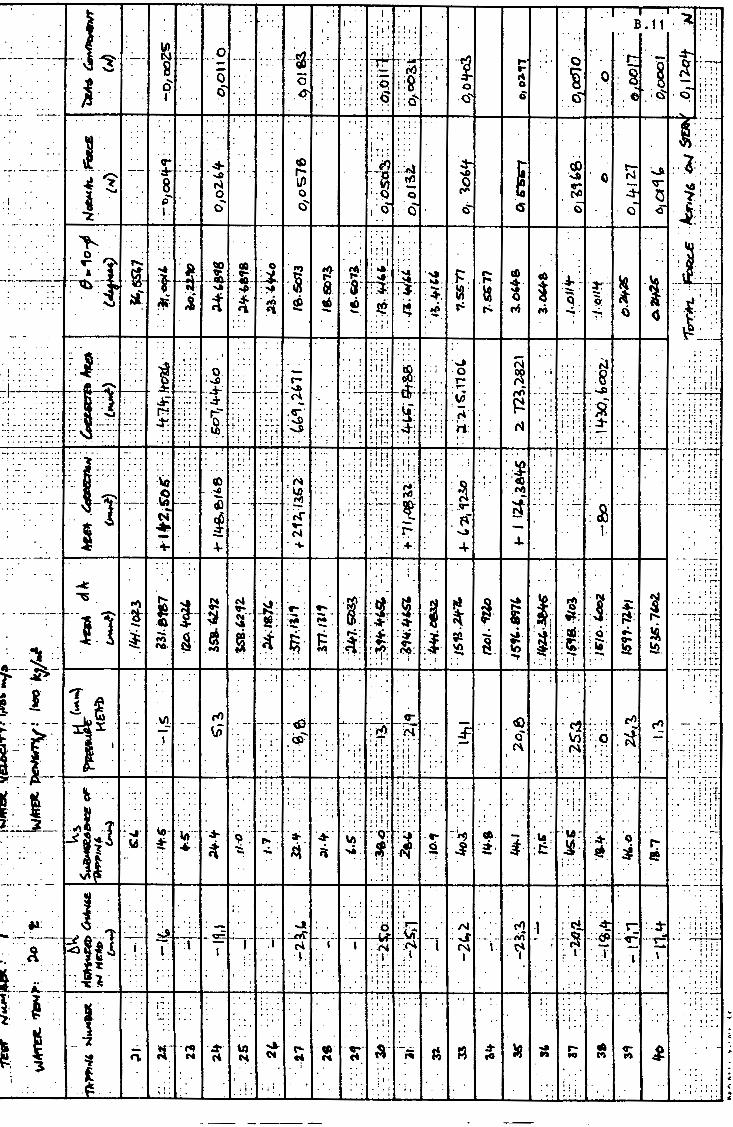
Univers
ity of
Cap
e Tow
n
...
"" --.-. -.. -._--+. ~--1- ti
. '·~ ~
. . . .,. . ~ . QQ CID .. o
t ~r.. ~ .... ;..., .... ·- ·-- -40- ........ . ... ~- ''."P
~ • .f- ·S. :;.,; ... " " ~. ~ . . '.,
. ·I· § M .. . .. I . .. .. .. '.::; • . : . ·:: .... :- .t: .: f .. ~:: .. ! !j!! ~ .. :~ ~ ... .. ~ ... 'i
. ''
I ~·!-:'.:::~=·:: ;:r· :1;..~ .... :~. ;: .~ :;;ijl~ ti:::;'..-~ 1-.·: .. :_.:_:·~] ·::T;r1 - -- .. , ~- t--- •c~ - •• -. -. -.-•• - _, - •• ~ •• ---,-,. -. r- ·.+-.'. . .. '"'' s • r
· • :·: .. : · · .. : ·. : : '. : : i . '. L- : ,·:. : : ..l. , • <" \I) ~ . ·, ', •. ·, '· ', - • · • .... r ~ ..,;;r- ·• 'f' .. I ·- ·'•• :·o ··•!j•·'• ~-=~·:· '.:::::: !'. :·~ ::: N :;:: 't'."- :~· , . ., 1:'!.; :~: .... ~· ,.,, ~ .. '.::;.~:.;-: •.••• t .......... ~-· ---· --·· ~- +;.;: .o. ~'.:: :~:; ·-~ ~:.j itl.r ;,.L; ·1:i ·~ N 1· 1 • :.l- ·i •• ~ .. p,·~:rt
• ~::·~::.:.::·:·.:_:-: :-: :~:·:· ·::· •• •• ,. :~ .. !.t, tt"1 ~ ;:;~ :1+; !~!•I·• ta'. ' 11 :,. .·'1·_:,~~,··!;_'•,'•.r -... ~·~_ .. _-_ ... _._ .. _ .. ~·~·-·-·-·-··~· ...... -· ...---1~·~··-+~l't-::_.~·~i_:_~;+-··--· ...... -+---+.-"~;~ .. ~·-·-"-+-__ ._...:_: +-·--l,__-+-...--1-·-·'~: ....... ·:_;~· -·-·_....~~-
• ::::-~:·::~:-.:::: :·:·~-: ... -· •. '.::; i1·l .... : I· ',-~l,.! 'lo !· i :•1 !~'.:,r·:~:_·
~ :tt' :~:~ ,i:_i .. •'?' t•lt· ,.,, :::: ,, • .• \t) ...
·.-~.- ~~-'.:-~:·_~_: ~.· '~-; ~-:~. ·""~~ ... .- - -~ ~·- _:f_:; !@ .. :::! tf!! :~: ::: :~ .:. -~-~. ~'.;;_ ::_~.:a -- ---. _).~.·.i_L.'..'.~.: ! .! - • ~ ---- ' • ~ ' ''t -~ ~ : -. ~ "' f
= J ..... "T" ,.. .• '.' . ; ... : "'T' ~
- -- ____ .. --- .. t----t---t--t---+--t--+---t--t---t--~.-.-. ,-t---1'---+--t--t-~--+--~-t----+--1 I , • o • ,_.-f
··;· ;i:!~ ~ ,.
I ·----~ -·i ~--~ .. ~ t--~'..t;: .. !:. ·~:~~;:-$. :~ ~ ~.· i ~:· l::l .. ~: ~ ::~~~~l . -- -----·: ·1. ,. :;: .. C) g: ·· ..a !!. :~ ~ IJ), ·~ ~ '1 "' .~I · · ·· · ·':L·~~
I : ! ~ ;;i <S: d f!· .4- t:: . .:; .~: :t.: ::;· :~ ~ ~ " .. ·;;!: :~: i . .-_i:'.Q: E ?9i ::1:L~! . ' ... . ....... l'4), ti ..-, ~ C\ ~ "' c;&· ·~· ~;·;to· ... ~ .. \r.I ~: :~· .., ~ ~ ., ..... . " ·-t : . . . . .. . . . . , . ; : !·: : . ' : . ' . "'."' ..,. : : .. I . ! ! ,. . :· :J'. ; ~:~ .. 4·---~ - t----+--+--ii---t---+--t--+-+-+---1..,_-+--+--t--+--+---+--. ~. f-,-, ,-,-+--if----+--t. --.---'-
......_ v~. . . '· ' '.. . . ! •; '. ,' I ~ ,.:i ,.
6 i 1 T~ . ~ -~·- .. . -13: .~· :J . -- ~~~~ :~ : :··· ~-~--- i#-~ ~ . '§ -' :.- §. ~:~ : ~ r'l :. · .. : .. :.:I!:·.:,.: . ~· ·r· -· !:'.. .. . .. ... :;: .. ., ..... ~ • • • • • I • 4 t t t ~ ! ! ~ ·• • ; . • · : ,"
1 . : ~ • • • ? • • :
. . ! : ! 1 ·~ ' i : ' . . . . ~ . . . I : ' ; i '. : : . ~-~ ··--+---~--+--+---11---+--+--+-~--+-+-....... i-o--+--t--+-~--+--+-...--t----+--t----t ..... _. ---
' ; ' • I ! j I l ' . . . . . . . • : ~ i ; :j . l.~·l \ . :.. ., .. ;1~1 .l!!: .. .. ::·: :;:; 1-:.· · .... 1.1.:.;_,1 • •. ';I J I ' 'l ')f I
. . I:' . '. ~ j~ t ; : ! : 1 • •;, : l: •I• I 1
~ ..., . 1' .... •1' f;ti :111 ···;,! --.· -:~~- ~ .... 5 ~:.... ~- &,>':- ·.;t. 9 ,- ~-: .• ·~. "' ~'.Q~: ;;· .... -:-·~ - ,... ·lA, ~\4~ . ~: ·~· .. -•. , -_ - JI 16 ~ • * " .. ~- ii ... ~· .~- -~ ~ i!· ' "'' ,~ -!!. ' ~ , -,, - ·-- .. --· .. - - - t--....... -+-+--it---+--+--t--+-+--+--1--.. +-, -. -t, --+-+---t--+--+-...-+---it--+--t---- --~
J .. : .! : ... - - ~ . . • • I . t: . ..'. ; : I
fol: - . . . : . - . . . . - J . . . : : 0 : ·~ . . ____ _,:._:;-- ~1~1. :. ~-;· ~7:f-""',-~· ....--+-·-r :~~-i~. - , .:;.; ~~ ~-1 C1. ' ·L ::1: ,I , -·1 ··: . ·.: .. ~· : .. · .. : ... .. ..;:;
!I: I ~ : ; • : . -- -- :._A-. : ' . .. .. '
{'. . I
l, '
· l" l
- "I
r::
. , I·
j j •
, 11: i ,. -·. , .
. ': !
. ,_ ' ; I• ':
''
: r-J .. J
N I
• . ••• ' ' •• '! •
: . '1 ·I : ·~ .. ~ : r: : · :t : -'. : '. i ~ ! ·-... -M - · --~ -.. {P-~r --~ -- ·.,...P,-.,. . I. ~ ' : ct- . f - - . ;:1:
I [' . . -~ .. \ .. . ; : : :
. : '. 1: .. ;
. I;.
.. ; : : !,
' • ' ~ • I • • • •t
• I • • ~ f
, • - •• 1t --..--- ......... . ; i ~ . : :
• : •• 1
.. 'I.•:•
• ·1 • •••

Univers
ity of
Cap
e Tow
n
c. 1
APPENDIX C
LOW PASS FILTER
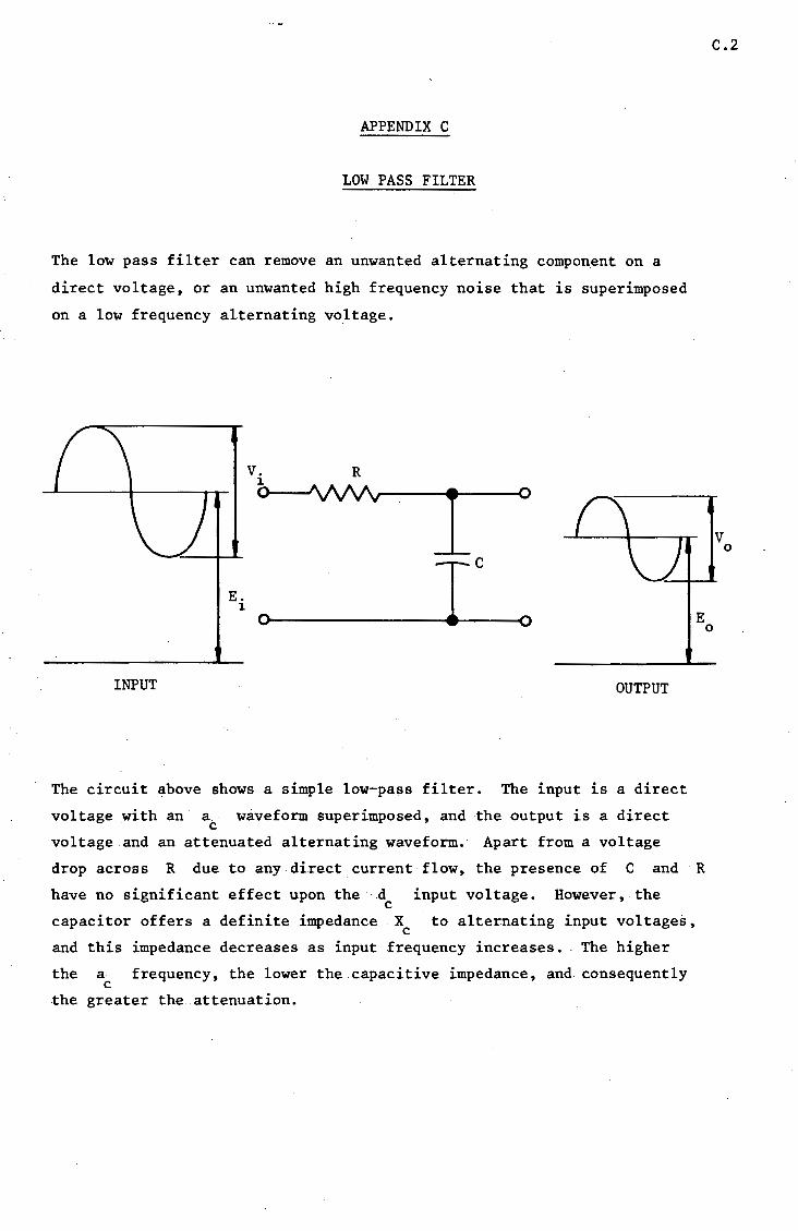
Univers
ity of
Cap
e Tow
n
APPENDIX C
LOW PASS FILTER
The low pass filter can remove an unwanted alternating component on a
direct voltage, or an unwanted high frequency noise that is superimposed
on a low frequency alternating voltage.
INPUT OUTPUT
The circuit above shows a simple low-pass filter. The input is a direct
voltage with an a . c
waveform superimposed, and the o~tput is a direct
voltage and an attenuated alternating waveform. Apart from a voltage
drop across R due to any.direct current·flow, the presence of C and
have no significant effect upon the d input voltage. However, the c
capacitor offers a definite impedance x to alternating input voltages, c
and this impedance decreases.as input frequency increases. The higher
the a c
frequency, the lower the.capacitive impedance, and consequently
the greater the attenuation.
C.2
E 0
R
v 0
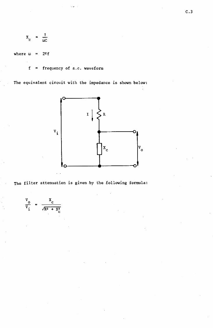
Univers
ity of
Cap
e Tow
n
x = c we
where w = 27Tf
f = frequency of a.c. waveform
The equivalent circuit with the impedance is shown below:
v. 1.
x c v
0
The filter attenuation is given by the .following formula:
v 0
v. 1.
= x c
/R2 + x2 c
C.3

Univers
ity of
Cap
e Tow
n
D.1
APPENDIX D
STRAIN'GAUGE BRIDGE THEORY
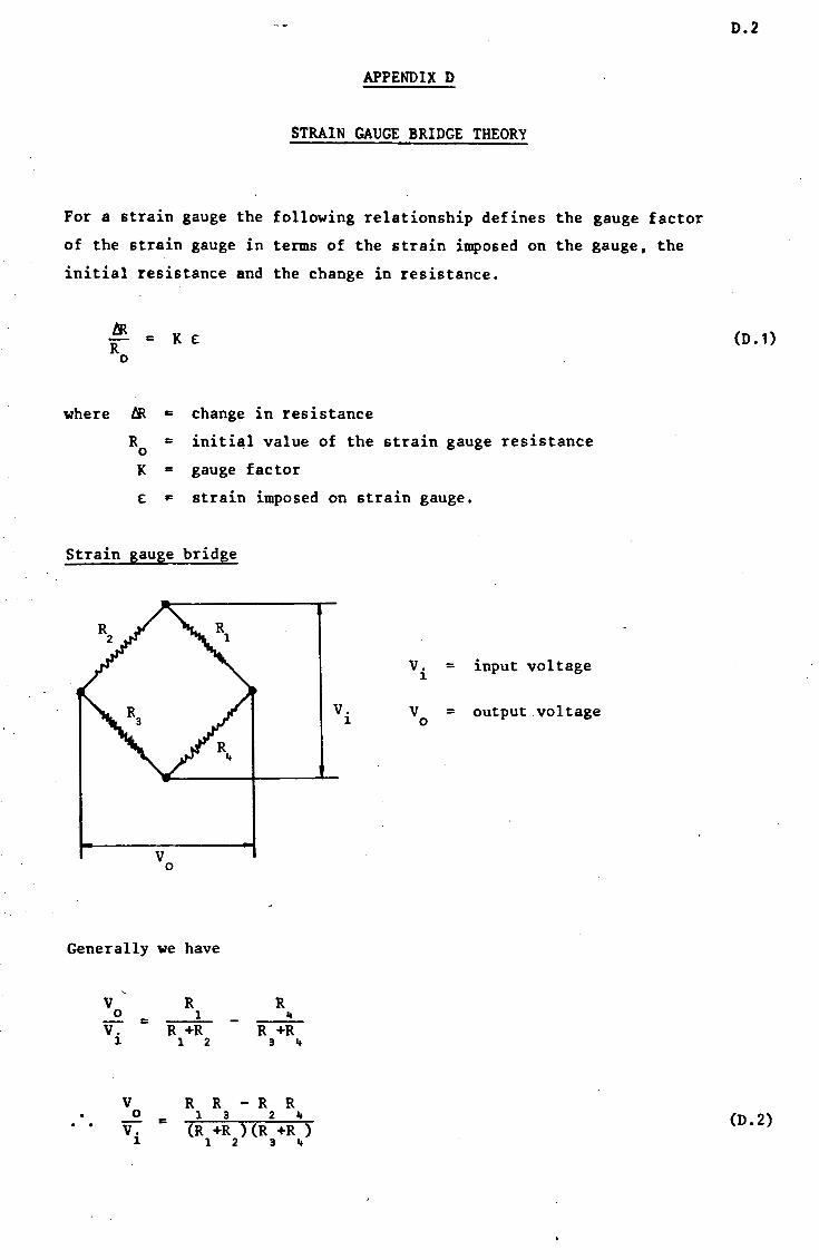
Univers
ity of
Cap
e Tow
n
APPENDIX D
STRAIN GAUGE BRIDGE THEORY
For a strain gauge the following relationship defines the gauge factor
of the strain gauge in terms of the strain imposed on the gauge, the
initial resistance and the change in resistance.
M R
0 = K E
where & = change in resistance
R = initi~l value 0
K = gauge factor
E "' strain imposed
Strain gauge bridge
v 0
Generally we have
v 0
v. = 1
v 0
v. 1
R l
R +R l 2
R It
R +R 3 It
R R - R R = l 3 2 It
(R +R )(R +R ) l 2 3 It
of the strain gauge resistance
on strain gauge.
V. = input voltage l.
Vi V0
= output voltage
D.2
(D .1)
(D. 2)
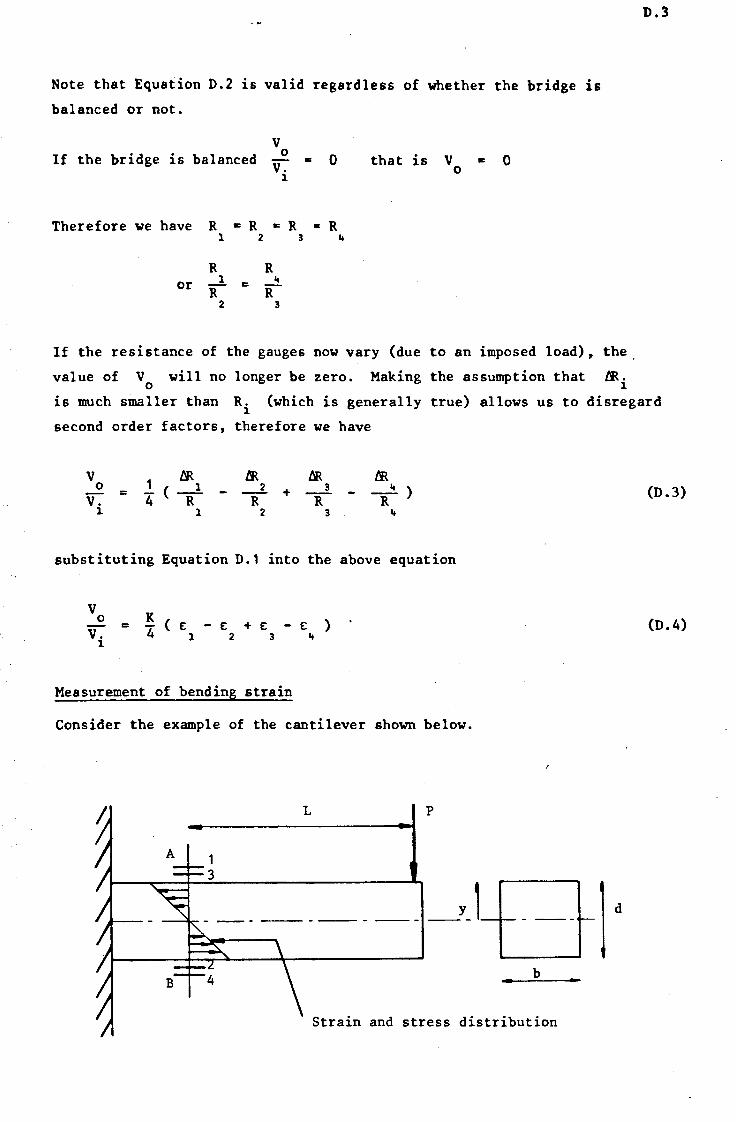
Univers
ity of
Cap
e Tow
n
Note that Equation D.2 is valid regardless of whether the bridge is
balanced or not.
If the bridge is balanced v
0 - c v.
l
0
Therefore we have R c R c R c R l 2 3 ..
R R or __!._ c: " R R
2 3
that is v 0
0
If the resistance of the gauges now vary (due to an imposed load), the
value of V will no longer be zero. Making the assumption that ~. 0 l
D.3
is much smaller than R. (which is generally true) allows us to disregard l
second order factors, therefore we have
v 0
v. l
= M.
1 ( _l 4 R
l
& - __ 2 +
R 2
M. __ 3 -
R 3
substituting Equation D.1 into the above equation
v 0 - = v. l
Measurement of bending strain
Consider the example of the cantilever shown below.
L p
------ _Y_, b
Strain and stress distribution
(D.3)
(D.4)
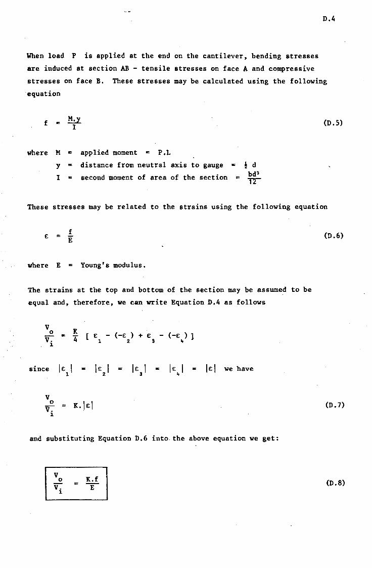
Univers
ity of
Cap
e Tow
n
D.4
When load P is applied at the end on the cantilever, bending stresses
are induced at section AB - tensile stresses on face A and compressive
stresses on face B. These stresses may be calculated using the following
equation
f c ~ I
where M c applied moment c P.L
y
I
= distance from neutral axis to gauge = second moment of area of the section =
i d bd3
T2
(D .5)
These stresses may be related to the strains using the following equation
£ =
where E
f E
= Young's modulus.
The strains at the top and bottom of the section may be assumed to be
equal and, therefore, we can write Equation D.4 as follows
v K 0
[ £ - (-£ ) + £ - (-£ ) ] = 4 v. 1 2 3 It 1
since I e: I = I e: I = le: I = le: I = le: I we have l 2 3 It
v 0
K. I e: I v. = 1
and substituting Equation D.6 into the above equation we get:
v 0
v. 1
K.f = --E
(D.6)
(D. 7)
(D.8)
Univers
ity of
Cap
e Tow
n
•
Therefore, the above expression gives the output voltage of the bridge
in terms of the gauge factor, stress at the section, Young's modulus
and the input voltage. This equation is used for design purposes only
and each bridge must be calibrated before experimental measurements are
made. Note that it is important that the strain gauges 1 and 3 and
D.5
gauges 2 and 4 are on opposite sides of the beam to ensure that Equation D.7
is valid •
1 B JUN 1987


![Research Article An Investigation on the Effects of Ship Sourced … · 2019. 7. 31. · air pollutants in Shanghai Port and identify the contribution from ship tra c emission [ ]](https://img.pdfslide.net/doc/110x75/60e2a392c9ae1d4e2f17cd95/research-article-an-investigation-on-the-effects-of-ship-sourced-2019-7-31.jpg)