Embed Size (px)
Citation preview
Report prepared for the Electricity Authority
An exploration of locational marginal
pricing at the distribution level in the New
Zealand context
Stephen Batstone, David Reeve, Toby Stevenson
29 June 2017


DLMP in the New Zealand context Page i
16 March 2018 11.24 AM Commercial in Confidence
About Sapere Research Group Limited
Sapere Research Group is one of the largest expert consulting firms in Australasia and a
leader in provision of independent economic, forensic accounting and public policy services.
Sapere provides independent expert testimony, strategic advisory services, data analytics and
other advice to Australasia’s private sector corporate clients, major law firms, government
agencies, and regulatory bodies.
Wellington
Level 9, 1 Willeston St PO Box 587 Wellington 6140 Ph: +64 4 915 7590 Fax: +64 4 915 7596
Auckland
Level 8, 203 Queen St PO Box 2475 Auckland 1140 Ph: +64 9 909 5810 Fax: +64 9 909 5828
Sydney
Level 14, 68 Pitt St Sydney NSW 2000 GPO Box 220 Sydney NSW 2001 Ph: +61 2 9234 0200 Fax: +61 2 9234 0201
Canberra
Unit 3, 97 Northbourne Ave Turner ACT 2612 GPO Box 252 Canberra City ACT 2601 Ph: +61 2 6267 2700 Fax: +61 2 6267 2710
Melbourne
Level 8, 90 Collins Street Melbourne VIC 3000 GPO Box 3179 Melbourne VIC 3001 Ph: +61 3 9005 1454 Fax: +61 2 9234 0201
For information on this report please contact:
Name: Toby Stevenson
Telephone: +64 49157616
Mobile: 021666822
Email: [email protected]

DLMP in the New Zealand context Page iii
16 March 2018 11.24 AM Commercial in Confidence
Contents
Glossary (TBC) .................................................................................................... v
Executive summary ........................................................................................... vii
1. Introduction ............................................................................................ 1
2. What is DLMP? ....................................................................................... 2
2.1 DLMP is a subset of Locational Marginal Pricing, and the boundaries
are arbitrary ................................................................................................... 2 2.2 The purpose of LMP is to provide efficient signals based on secure
optimal economic dispatch ......................................................................... 3 2.3 Defining the distribution-transmission boundary is fundamental ....... 3
3. Definitions of transmission and distribution .......................................... 5
3.1 Distribution – key characteristics .............................................................. 5 3.2 Transmission, Distribution, and the role of voltage ............................... 6 3.3 Firm definitions for the purpose of network models............................. 7
3.3.1 AC Modelling Equations .............................................................. 8 3.3.2 DC Modelling Approximations .................................................. 8
3.4 Identifying transmission nodes and lines ............................................... 11 3.5 Identifying distribution nodes and lines ................................................. 12
3.5.1 Distribution substation ............................................................... 13 3.5.2 Secondary distribution network ................................................ 13 3.5.3 Primary distribution network .................................................... 13 3.5.4 Zone substation ........................................................................... 13 3.5.5 Sub-transmission ......................................................................... 14
3.6 Loop, mesh and radial ............................................................................... 15
4. Distribution – Depth, Granularity and Definition of Nodes/Zones ..... 18
4.1 Impact on granularity of prices – potential number of nodes ............ 19 4.2 Assessment required to determine suitability of DC approximation 21 4.3 Information required for LMP modelling .............................................. 22
5. Modelling considerations for calculating DLMP prices ....................... 24
5.1 DCOPF models.......................................................................................... 24 5.2 Alternative to DCOPF models: ACOPF ............................................... 24
5.2.1 Non-Linearity and non-convexities .......................................... 25 5.2.2 Modelling constraints for congestion prices ........................... 27 5.2.3 Summary – Modelling Options ................................................. 28 5.2.4 Bidding, Offering and Prices ..................................................... 30
6. Institutional Arrangements ................................................................... 32
6.1 Implementing DLMP under a DSO ....................................................... 34 6.1.1 Establishing a DSO ..................................................................... 35
6.2 Model 1 - TSO and Distribution System Operator(s) only ................. 36
Page iv DLMP in the New Zealand context
Commercial in Confidence 16 March 2018 11.24 AM
6.3 Model 2 - TSO/DSO and ‘franchised’ aggregators using an approved
model............................................................................................................ 36 6.4 Model 3 - Private operators using proprietary locational models but
meeting set standards ................................................................................ 37 6.5 Model 4 - Private operators using proprietary locational models with
communication protocols ......................................................................... 37
7. Options assessed in terms of tasks and complexity.............................. 39
7.1 Investigations required for each broad option ...................................... 40
Appendices No table of contents entries found.
Tables Table 1 - assessment of X/R ratio for various voltages in the Belgian transmission
network 11
Table 2 - Illustration of line characteristics 12
Table 3 19
Table 4 - Distribution networks and characteristics for LMP modelling 21
Figures Figure 1 - Summary of electrical network ix
Figure 2 Current and possible distinction between the reach of the TSO and DSO(s)
and the role of DLMP xii
Figure 1 - Vectorised representation of Z with an X/R ratio of 4 9
Figure 2 - Vectorised representation of Z with an X/R ratio of 2 10
Figure 3 - Summary of electrical network 14
Figure 4 - Stylised loop circuits 15
Figure 5- Stylised Radial Network 16
Figure 6 - Zone substation node and implied zone 19
Figure 7 - ICP nodal pricing with zone aggregation 20
Figure 8 - solution space for an ACOPF 25
Figure 9 Current and possible distinction between the reach of the TSO and DSO(s)
and the role of DLMP 32
DLMP in the New Zealand context Page v
16 March 2018 11.24 AM Commercial in Confidence
Glossary
X/R ratio The ratio of series inductive reactance to series resistance in a power line,
a key characteristic for determining the eligibility of AC power lines for
DC approximation analysis
LMP Locational Marginal Pricing is a range of pricing techniques that establish,
to greater or lesser degrees of accuracy, the marginal cost of consumption
(price) at different locations in an electricity network.
TLMP Transmission Locational Marginal Pricing, LMP techniques for networks
that have the electrical characteristics of transmission
DLMP Distribution Locational Marginal Pricing, LMP techniques for networks
that have the electrical characteristics of distribution
ICP An Installation Control Point is one of the following:
(a) a point of connection at which a customer installation is connected to
a network other than the grid:
(b) a point of connection between a network and an embedded network
(c) a point of connection between a network and shared unmetered load
TSO A Transmission System Operator operates a transmission network which,
in the context of TLMP, means operating the TLMP model, dispatching
assets and coordinating security.
DSO A Distribution System Operator operates a distribution network which, in
the context of DLMP, means operating the DLMP model, dispatching
assets and coordinating security.
DC network DC networks are networks of electricity lines that run on direct current,
typically at one voltage. They are simpler than AC networks to do power
flow analysis on.
AC network AC networks are networks of electricity lines that run on alternative
current, and are used for networks that operate at many voltages. Because
of using AC these networks produce reactive power, which is a
complicating factor in power flow analysis.
DCOPF model
DC Optimal Power Flow modelling is the leading method of doing
TLMP. It is based on approximating an AC network as a simplified DC
network and using linear or mixed integer programming techniques to
optimise for least cost or net societal benefit. It also produces locational
marginal prices.
ACOPF model
AC Optimal Power Flow modelling is being investigated as the leading
method of doing DLMP. It is based on a model which better represents
AC network behaviour than a DC approximation does. It uses non-linear
techniques to optimise for least cost or net societal benefit. Techniques
for producing locational marginal prices from these models are also being
investigated.

DLMP in the New Zealand context Page vii
16 March 2018 11.24 AM Commercial in Confidence
Executive summary
Changes in the way electricity is generated and consumed as a result of technology and
innovation are well documented. Consumers can now invest in small scale generation and
battery storage and have the ability to shift their net load or allow aggregators to control their
load to a greater degree than has been the case up until now. The shift of decision making
down to the consumer level is also encouraging innovation for retailers and aggregators.
They are increasingly able to compete with distributors to commercialise consumers’
flexibility. This fragmentation of decision making and shifts in commercial opportunities are
changing the nature of the electricity market.
Consumers are no longer the end of a supply chain that begins with generation and ends
with distribution to the meter. An increasing portion of the supply chain can now be
categorised as distributed energy resources (DER). DER can meet local electricity demand
in direct competition with electricity produced remotely and transported over the
transmission and distribution networks. DER can also be a new source of reserves and other
ancillary services. This development raises the question of whether a more granular electricity
nodal price signal, applied at nodes within the distribution network, would promote efficient
investment in and efficient use of distribution network assets and DER and promote more
efficient consumption decisions.
Scope However, this paper does not seek to address the question of whether more efficient
outcomes would occur from greater granularity and depth of nodal pricing. Rather, we were
asked to explore the practicalities of applying locational marginal pricing at distribution level.
This is an exploratory paper which considers:
(a) the practicable options to implement locational marginal pricing at the distribution
level in NZ, including a description of how these options could operate in practice
(b) any limits on the extent of location marginal pricing, including geographical limits
(e.g. how deep into the distribution network could it extend?) and other key limits
(c) the main obstacles to implementation of locational marginal pricing at the
distribution level, including high-level thoughts on how they could be overcome
(d) potential changes to current market arrangements, including to systems, processes
and regulatory arrangements, that might be required to implement each option
(e) the tasks involved and possible costs likely to be incurred in implementation of
each practicable option (at a high level only)
(f) the length of time likely to be required for implementation (high-level estimate
only).
This paper addresses (a) to (d) but does not address (e) and (f). Midway through the work it
was agreed with the Authority that a fulsome understanding of the issues in (a) to (d) was the
critical point and that matters raised under that consideration would have to be resolved
before the shape of what would be implemented could be meaningfully considered.
Page viii DLMP in the New Zealand context
Commercial in Confidence 16 March 2018 11.24 AM
Technical considerations Distribution Locational Marginal Pricing (DLMP) is a subset of Locational Marginal Pricing
(LMP). LMPs are the outcome of optimising electricity resources subject to network
constraints). When the optimisation is solved it is not critical that implied prices are published,
but for prices to be a tool of any value (from a signalling perspective) they must be intended
to be used for transacting energy.
Historically, LMP has been a product of an optimisation of generation and demand response
at the transmission grid level, which is known as the Scheduling, Pricing and Dispatch model
(SPD). In the context of this paper LMP at transmission level is also referred to as TLMP.
The GXP boundary which historically defined TLMP nodes was based on a choice of nodes
and links that had historically been part of the state’s bulk supply arrangements, rather than
any logic informed by the efficiency of price signals.
TLMPs do not necessarily provide efficient marginal signals for losses and congestion on the
network beyond the GXP. While TLMPs are reliably efficient short-run signals for grid-
connected generators and consumers, the use of an average loss factor in the distribution
network means that we cannot be confident that we have efficient marginal signals for losses
and congestion on the network beyond the GXP, i.e., for distribution-connected customers.
Further, we cannot be confident that the current signals reflect losses and congestion at any
point in time.
At some point on the continuum of transmission assets through to low voltage distribution
assets the technical characteristics that impact on efficient investment and operation change.
These changes have implications for the decision variables, the modelling approach and, in
turn, the merits of producing prices from the resulting optimisation models. SPD, the model
used to produce TLMPs, currently relies on a DC approximation of the electrical system it
represents, which provides a range of important advantages which go to the heart of
efficient, reliable market clearing prices.
The notion of optimising the distribution system with a DLMP approach would also have
implications for institutional arrangements. The difference between solving for transmission
optimisation and distribution optimisation are summarised below.
Transmission tends to:
• be higher voltage
• be more interconnected
• have more active and distributed voltage sources (i.e. generation)
Distribution tends to:
• be lower voltage
• be more radial
• have less, or more concentrated, active voltage sources (i.e. generation and GXP)1
1 We note that technology is changing the third characteristic for distribution.
DLMP in the New Zealand context Page ix
16 March 2018 11.24 AM Commercial in Confidence
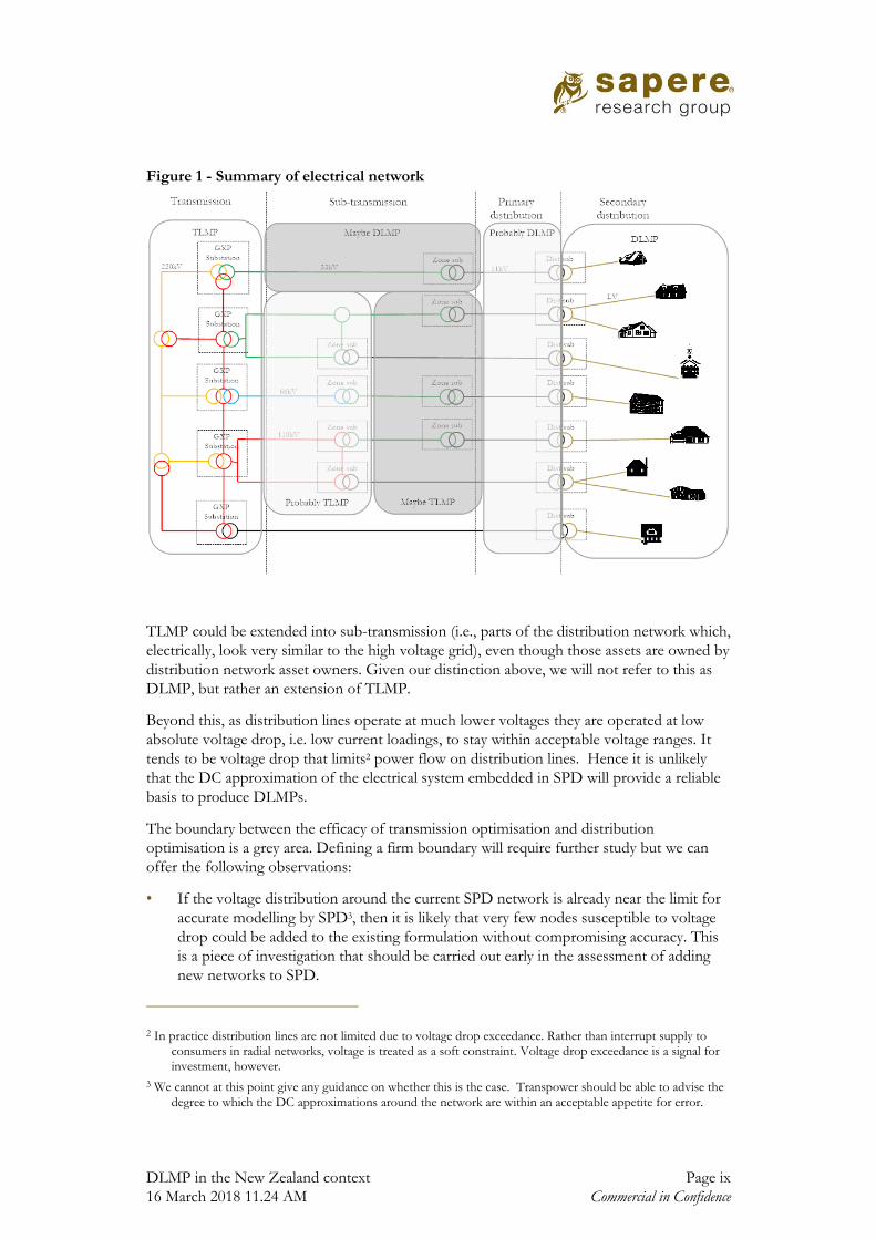
Figure 1 - Summary of electrical network
TLMP could be extended into sub-transmission (i.e., parts of the distribution network which,
electrically, look very similar to the high voltage grid), even though those assets are owned by
distribution network asset owners. Given our distinction above, we will not refer to this as
DLMP, but rather an extension of TLMP.
Beyond this, as distribution lines operate at much lower voltages they are operated at low
absolute voltage drop, i.e. low current loadings, to stay within acceptable voltage ranges. It
tends to be voltage drop that limits2 power flow on distribution lines. Hence it is unlikely
that the DC approximation of the electrical system embedded in SPD will provide a reliable
basis to produce DLMPs.
The boundary between the efficacy of transmission optimisation and distribution
optimisation is a grey area. Defining a firm boundary will require further study but we can
offer the following observations:
• If the voltage distribution around the current SPD network is already near the limit for
accurate modelling by SPD3, then it is likely that very few nodes susceptible to voltage
drop could be added to the existing formulation without compromising accuracy. This
is a piece of investigation that should be carried out early in the assessment of adding
new networks to SPD.
2 In practice distribution lines are not limited due to voltage drop exceedance. Rather than interrupt supply to
consumers in radial networks, voltage is treated as a soft constraint. Voltage drop exceedance is a signal for investment, however.
3 We cannot at this point give any guidance on whether this is the case. Transpower should be able to advise the
degree to which the DC approximations around the network are within an acceptable appetite for error.
Page x DLMP in the New Zealand context
Commercial in Confidence 16 March 2018 11.24 AM
• Notwithstanding this, it is likely that typical X/R ratios for distribution lines
downstream of current GXPs to the operating voltage of 66kV are likely to be
acceptable for an expanded TLMP; or, if they do have low X/R ratios, then they are
likely to be relatively short and have low voltage drop. These lines can probably be
categorised as transmission for the purposes of TLMP and could then be added to
SPD, subject to it being tested for its existing limits of accuracy.
• Below operating voltages of 66kV is a grey area.
• We are confident in assessing LV networks, and secondary distribution networks
generally, as not meeting the requirements of DC approximation. They would require
AC techniques to implement DLMP. Generally, the 11kV network is managed to a
voltage profile integrated with the voltage profile of the LV network. Overall, we
suspect that the 11kV network, and the primary distribution network generally, will not
meet the criteria for DC approximation.
If any lines and substations are considered for the implementing of LMP (regardless of
whether TLMP or DLMP) they will require information to an appropriate level of detail or
standard. The following would need to be done.
• Survey any lines and substations for which there is insufficient information
• Install all required telemetry where it doesn’t currently exist
• Install code compliant metering or establish an alternative that is acceptable for
settlement. Having considered the merit of extending TLMP to sub transmission the
question of whether to pursue DLMP beyond that requires a different approach.
Modelling considerations Once the nature of the electrical system is understood, there are some very real modelling
considerations. The current market setup (SPD as a DC-approximated optimal power flow
model) ensures that robust optimal locational marginal prices can be produced reliably, and
market participants can be confident that their power transactions are based on efficient
signals. As we look to move beyond the current GXP boundary though:
• For that part of the sub-transmission network where DC approximations are still
appropriate, LMP prices can be robustly produced by DC Optimal Power Flow
(DCOPF) models (as they are for SPD). Practically speaking, this would possibly be
most efficiently done by incorporating them into the existing SPD model, although that
is by no means a fait accompli: SPD may have limited “capacity” (in terms of impact on
overall model performance) for a number of new nodes, and/or it may be considered
more desirable to model these parts of the network using new system operators.
• For the parts of the network beyond this, AC Optimal Power Flow (ACOPF) models
would be the ideal, but we believe it is unlikely that they are sufficiently developed to
robustly produce LMPs. Currently, this is a very real impediment to the
implementation of DLMP. In time, however, this may be addressed.
• As an initial step, an ex-post (or real-time) marginal loss factor pricing approach could
be adopted, as a more sophisticated version of the current average “loss factor”
approach used for the settlement of purchases and distributed generation. Equally, an
administered congestion price approach could be used using smart meter data, where
constraints may reflect thermal, power quality or voltage limitations.
DLMP in the New Zealand context Page xi
16 March 2018 11.24 AM Commercial in Confidence
• These are shortcuts in the sense that they do not require full ACOPF optimisation
models to be developed, although it may draw on some of the AC equations for
marginal losses.
• While this may seem a very small step towards proper DLMP (losses and congestion
with optimal dispatch), the relatively higher level of losses on the distribution network
will still provide a strong locational signal.
• We reinforce though, that – if the current Code approach of average loss factors is
taken – these prices will not be “optimal” in any given period. This will especially be
true if the resulting loss-based DLMP prices instigate a response (e.g., installation of
DER), which will not be picked up by the averaging until the next calibration (which
could include real-time calibration, but not forward-looking).
• We note that by moving to marginal losses (and congestion) on the distribution
network (as with constraints) a settlement surplus will be created (in the same way as it
is created on the transmission grid). An allocation of this surplus will have to be
determined.
• The choice between depth, granularity and definition of node/zone at distribution level
is a choice between the level of differentiation to be signalled through the network, the
number of prices that results and the net benefits of signalling LMP to a specific
location or ICP.
• In practical terms, the consequences of the choice can be viewed in terms of the
number of new nodes that would be created. For example:
A nodal model down to zone substation could create approximately 1,200 new
nodes, where each new nodal price would effectively become a zonal price for
around 1,600 ICPs on average.
Similarly pushing a nodal model down to the distribution substation level would
create 187,000 new nodal prices, where each new node would effectively become a
zonal price for 11 ICPs on average.
By way of comparison, LMP markets in North American have tens of thousands of nodes.
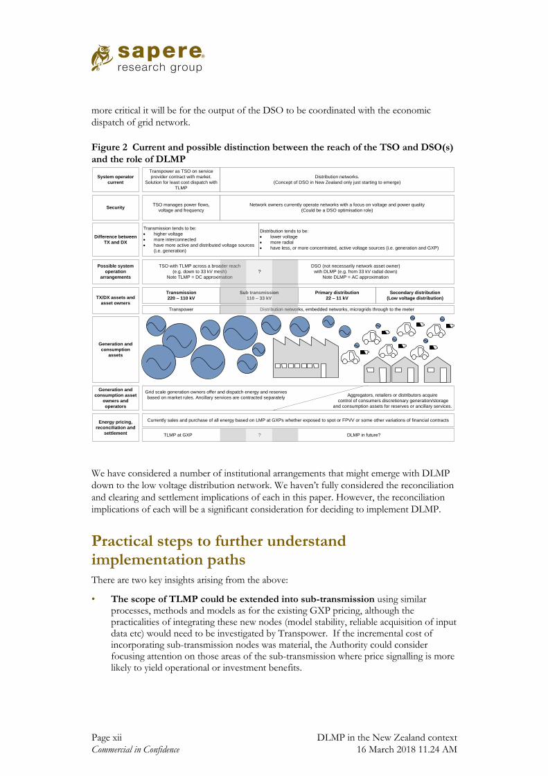
Governance considerations The governance and practical implications of extending TLMP, versus introducing DLMP,
are quite different. With TLMP the Code is already well established although there may be
implications resulting from the broadening of the asset ownership domain. With DLMP the
question is more to do with whether there is central coordination over the price formation
process and whether that leads to the establishment of a distribution system operator (DSO)
role independent of the distribution asset ownership in the same way the Transpower’s
System Operator division is kept operationally separate from Transpower as the grid owner
at present.
The need to account for network common quality and security, with multiple providers of
services, and in the context of maximising economic benefit, will require a DSO role – in
some form - to be actively pursued. At the very least, even if the chosen philosophical
approach was to purely rely on consumers (or their service providers) responding to DLMP
price signals (rather than the formal establishment of platforms) it begs the questions of who
is going to calculate these prices (and how). The more active the DSO management the
Page xii DLMP in the New Zealand context
Commercial in Confidence 16 March 2018 11.24 AM
more critical it will be for the output of the DSO to be coordinated with the economic
dispatch of grid network.
Figure 2 Current and possible distinction between the reach of the TSO and DSO(s)
and the role of DLMP
We have considered a number of institutional arrangements that might emerge with DLMP
down to the low voltage distribution network. We haven’t fully considered the reconciliation
and clearing and settlement implications of each in this paper. However, the reconciliation
implications of each will be a significant consideration for deciding to implement DLMP.
Practical steps to further understand implementation paths There are two key insights arising from the above:
• The scope of TLMP could be extended into sub-transmission using similar processes, methods and models as for the existing GXP pricing, although the practicalities of integrating these new nodes (model stability, reliable acquisition of input data etc) would need to be investigated by Transpower. If the incremental cost of incorporating sub-transmission nodes was material, the Authority could consider focusing attention on those areas of the sub-transmission where price signalling is more likely to yield operational or investment benefits.
Transmission
220 – 110 kV
Sub transmission
110 – 33 kV
Primary distribution
22 – 11 kV
Secondary distribution
(Low voltage distribution)
Transmission tends to be:
· higher voltage
· more interconnected
· have more active and distributed voltage sources
(i.e. generation)
Distribution tends to be:
· lower voltage
· more radial
· have less, or more concentrated, active voltage sources (i.e. generation and GXP)
TX/DX assets and
asset owners
Generation and
consumption asset
owners and
operators
System operator
current
Transpower Distribution networks, embedded networks, microgrids through to the meter
Transpower as TSO on service
provider contract with market.
Solution for least cost dispatch with
TLMP
Distribution networks.
(Concept of DSO in New Zealand only just starting to emerge)
TSO with TLMP across a broader reach
(e.g. down to 33 kV mesh)
Note TLMP = DC approximation
DSO (not necessarily network asset owner)
with DLMP (e.g. from 33 kV radial down)
Note DLMP = AC approximation
Possible system
operation
arrangements
SecurityTSO manages power flows,
voltage and frequency
Network owners currently operate networks with a focus on voltage and power quality
(Could be a DSO optimisation role)
Energy pricing,
reconciliation and
settlement
Difference between
TX and DX
Generation and
consumption
assets
?
Currently sales and purchase of all energy based on LMP at GXPs whether exposed to spot or FPVV or some other variations of financial contracts
TLMP at GXP DLMP in future?
Grid scale generation owners offer and dispatch energy and reserves
based on market rules. Ancillary services are contracted separatelyAggregators, retailers or distributors acquire
control of consumers discretionary generation/storage
and consumption assets for reserves or ancillary services.
?
DLMP in the New Zealand context Page xiii
16 March 2018 11.24 AM Commercial in Confidence
• Full DLMP based on economic optimisation at distribution level is impractical at this time due to the lack of reliable optimisation methods. However, coarse approximations to distribution LMPs are possible, although, depending on how dynamically these approximations are calibrated and applied, these may not provide material efficiency gains over the status quo.
There is inevitably a preliminary investigation phase where many of the key questions raised
in this paper would be more rigorously assessed. We outline the high-level components of
that investigation:
If the Authority wished to extend TLMP into the sub-transmission network, it would need to:
• Determine an appetite for error, in the New Zealand network context, inherent in DC
approximations
• Carry out an empirical study of sub-transmission (to delineate the grey area) starting
with >66kV, remaining sub-transmission mesh, remaining sub-transmission radial, and
(if results are favourable) maybe 11kV mesh to determine the suitability for DC
approximations
• If the Authority wanted to implement LMP in those parts of the network that satisfy
the criteria for DC approximation via an expansion of SPD, it would need to carry out
an empirical study of SPD to:
Test whether SPD has the capability to incorporate new nodes and remain within
the appetite for error
Based on the allowable error, define the X/R and flat voltage criteria for inclusion
to SPD.
• If SPD cannot be acceptably expanded, and/or the Authority wishes to pursue a
different governance model, that model would need to be designed with a separate
DCOPF(s).
• Determine how required network information will flow between asset owners and the
TSO
Notwithstanding the difficulties with security-constrained optimal dispatch in the
distribution network, if the Authority wanted to pursue DLMP in the “true” distribution
network, it would need to:
• Assess the full governance and operating implications of DLMP down to low voltage
distribution. This includes the potential for the establishment of distribution system
operator(s), and the various models for how they may interface with private aggregators
and smart grid optimisation schemes, such as peer-to-peer distribution services and
virtual power plants
• Keep a watching brief on global developments in smart grids and the use of ACOPF
for DLMP.
• Investigate the practicality, and potentially modelling, of marginal loss approximations
between the defined TLMP boundary and the pricing zone.
• Investigate the practicality, and potentially modelling, of administered congestion
pricing using smart meter information to reflect congestion – whether as a result of

Page xiv DLMP in the New Zealand context
Commercial in Confidence 16 March 2018 11.24 AM
thermal, power quality or voltage limitations, between the defined TLMP boundary and
the pricing zone.
For either of the above implementation paths, the Authority would also need to investigate:
• The available information on network assets required for construction of either a
DCOPF, ACOPF or any other approximation used. This would inform an assessment
of the practicality for our two options, i.e., whether any of the following would be
required:
(g) A survey any lines and substations for which there is insufficient information
(h) Installations of all required telemetry where it doesn’t currently exist
(i) Installation code compliant metering to every zone substation, and possibly on to
every 11kV feeder circuit
• Investigate required Code changes, especially around clearing, settlement and
reconciliation, as well as grid definition and requirements for SPD
• Determine how any settlement surplus arising from the new nodes is dealt with
DLMP in the New Zealand context Page 1
1. Introduction
The Electricity Authority is exploring whether a more granular electricity nodal price signal
that applies at nodes within the distribution network would promote efficient investment in
and efficient use of distributed energy resources and distribution network assets and
promote more efficient consumption decisions. Distribution Locational Marginal Pricing
(DLMP) is being discussed because the level of discretionary and programmable load,
storage and/or generation devices is increasing in the distribution network. With the
potential for two-way flows (from storage and small scale generation), new methods for
congestion management and the need to coordinate many dispatchable devices arise.
We were asked to explore the practicalities of DLMP. Before doing so, we observe that the
degree to which the current model of nodal pricing (which we refer to as Transmission
Locational Marginal Pricing, or TLMP) has been applied historically coincides with network
asset ownership, and that the boundary between DLMP and TLMP may be better located at
a different point.
This paper explores, in more detail, what DLMP is, and the practical considerations and
tasks that need to be taken into account when considering whether and how it is
implemented, including the institutional arrangements that should be considered as part of
implementation. We will also comment, at a high level, on what these practical
considerations mean for the complexity of implementation, and the length of time it might
take.
Page 2 DLMP in the New Zealand context
2. What is DLMP?
The concept of Distribution Locational Marginal Pricing (DLMP) is a relatively recent
concept4.
The motivation for DLMP stems from the fact that there are potential benefits from price
signals reflecting the short-run marginal costs of distributing electricity through the network
beyond the existing LMP boundary (the Grid eXit Point, or GXP), in the same way that
TLMP currently reflects the short-run marginal costs associated with the high voltage grid.
This would potentially add economic dispatch to the network companies’ current efforts in
respect of security management, with the requisite computer optimisations and the potential
to publish prices that give efficient signals.
2.1 DLMP is a subset of Locational Marginal Pricing, and the boundaries are arbitrary
Fundamentally DLMP should be seen simply as a subset of Locational Marginal Pricing,
popularised by Schweppe (1992)5. The fact that we now highlight “Distribution” LMP
simply reflects that the implementation of LMP, historically, has focused on what is
understood as the transmission grid. Technically, countries that claim to have implemented
LMP have (as far as we are aware) actually implemented Transmission Locational Marginal
Pricing (TLMP).
However, the Grid eXit Point (or GXP) boundary which historically defined TLMP nodes
was based on a choice of nodes and links that had historically been part of the state’s bulk
supply arrangements (known as the “national grid”, i.e. Transpower’s asset base).
In New Zealand, the transmission grid was developed by the state and was then passed into
the ownership of Transpower (although still owned by the state). However, the delineation
between state ownership and the distribution networks (which were developed under local
power boards) was based on asset ownership, and so some power board assets (which have
since become Electricity Distribution Businesses, or EDBs) are more transmission than
distribution. These transmission-like assets that are owned by distributors are referred to as
sub-transmission.
4 Although we discovered that John Kaye of the University of NSW explored the concept in a publication in
1994. L. Murphy, R. J. Kaye, and F. Wu, “Distributed spot pricing in radial distribution systems,” IEEE
Trans. Power Syst., vol. 9, no. 1, pp. 311–317, Feb. 1994.
5 Schweppe, F.C., Caraminis, M.C., Tabors, R.D., Bohn, R.F., 1988. Spot pricing of electricity. Kluwer.
DLMP in the New Zealand context Page 3
2.2 The purpose of LMP is to provide efficient signals based on secure optimal economic dispatch
It is important to remember that the purpose of LMP is to create price signals that reflect the
optimal dispatch the system to maximise net societal benefit, which includes meeting
economic reliability. These prices are used to settle wholesale sales and purchases of
electricity. This incentivises, ideally, short and long run operations and investment decisions
consistent with the societal objective. From Hogan (2014)6:
“To achieve the intended outcomes of reliability and economic efficiency, it is important
to have efficient prices that are consistent with the objectives and operation of the
underlying system.”
Drawing on Hogan, for the purposes of this study, it is important to reinforce that in
electricity markets, where secure dispatch is both a complex undertaking and a primary
objective, efficient prices are commensurate with some sort of economic optimisation. This
is precisely how New Zealand’s wholesale market is managed: SPD is an economic dispatch
model, which has the objective of maximising net societal benefit (which reduces to
minimising cost with demand certainty) whilst preserving security. The desired outcome of
the model is intended to be consistent with the Authority’s statutory objective under the
Electricity Industry Act 2010.
Based on this optimisation, as Schweppe et al demonstrated mathematically, the shadow
prices7 on the power balance constraints at each GXP in SPD as the most efficient prices to
be paid by purchasers, and paid to generators. These are the prices we publish as nodal
prices.
2.3 Defining the distribution-transmission boundary is fundamental
Presently, wholesale transactions are settled at an efficient marginal price that is calculated
for the GXP, which is then adjusted by an average loss factor to a location proximate to the
customer’s (generator, consumer, or storer) premises. While current LMPs are reliably
efficient short-run signals for grid-connected generators and consumers, the use of an average
loss factor means that we cannot be confident that we have efficient marginal signals for
losses and congestion on the network beyond the GXP, i.e., for distribution-connected
customers.
6 “Electricity Market Design and Efficient Pricing: Applications for New England and Beyond” – William W.
Hogan (June 2014)
7 The shadow price, or dual variable, is a measure of the rate of change in total system cost for a small change in
demand at a particular GXP, thus exactly representing the short-run marginal cost
Page 4 DLMP in the New Zealand context
The materiality of this is a question beyond the scope of this paper. But, as outlined above,
the context for DLMP is the anticipation of a world where there are potentially multiple
participants, decentralised and dispersed, who – either through behavioural response or
automation – are driven by (amongst other things) the price that is used for their electricity-
related transactions. The question is to what extent can (and should8) we push the
locational-reflectivity of prices beyond the existing GXP boundary, and what would be
required to do so.
However, care is required here with terminology. We should not default to a categorisation
that DLMP is any LMP approach beyond the current set of GXPs. Since LMPs are the
result of an economic optimisation, we need to be careful that we consider the salient factors
involved in this optimisation, in order to ensure that the prices are “efficient” and thus
sending a signal to customers that reflects a maximisation of economic welfare. We will
outline below that some of the critical factors in secure, economic dispatch on the
transmission network are not the same as those factors that must be considered in many
parts of the network owned by distribution companies. If the critical factors are different,
then the optimisation which produces LMPs may, at some boundary, need to be different.
Hence, from the perspective of producing robust and efficient prices, the boundary between
the two is largely a technical one, not an asset ownership one as is currently the case9.
As explained below the historical delineation is not a useful starting point for this assessment
and therefore true DLMP may not commence at this asset ownership boundary. The space
in between may be considered as an extension of TLMP.
We make this distinction not to be pedantic. But, in many ways, it clarifies the thinking
about DLMP and the roles of potential distribution system operators, and “unhinges” these
from historical decisions about asset ownership. These institutional realities can be re-
introduced where relevant, but we believe it is important to get the logic behind the pricing
calculation clear first.
8 Although we reinforce that, for this paper, whether this should occur is beyond scope, and we make no
recommendation in this respect.
9 Although this should not be read to imply that asset ownership is irrelevant: quite the opposite. As discussed
later, even pushing TLMP just inside the network ownership boundary may result in Transpower (as System
Operator) having up to 29 new counterparties, in terms of telemetry, line characteristics, switching etc.
DLMP in the New Zealand context Page 5
3. Definitions of transmission and distribution
For the purpose of DLMP we use the following definition of transmission and distribution.
Transmission is the network where the predominant restriction on line capacity is thermal
capacity; and the primary operational objective is asset utilisation subject to security.
Distribution is the network where the predominant restriction on line capacity is voltage
drop; and the primary operational objective is meeting service standards subject to thermal
limits.
Transmission tends to:
• be higher voltage
• be more interconnected
• have more active and distributed voltage sources (i.e. generation)
Distribution tends to:
• be lower voltage
• be more radial
• have less, or more concentrated, active voltage sources (i.e. generation and GXP)10
To understand the reason for our definitions of transmission and distribution above it is first
necessary to understand the relevant differences between transmission and distribution.
3.1 Distribution – key characteristics In an electric power system, the specific definition of distribution is that part, or those parts,
of the system that distribute electricity to households and businesses at a safe voltage
(sometimes known as the utilisation voltage). A safe voltage for most households and
businesses (those that don’t have the expertise or need to take supply at high voltage) is quite
low. In New Zealand, the nominal voltage for supply to normal installations (i.e. Installation
Control Point) is 230/400V. This voltage is too low to transmit much power or transmit it
very far and the voltage must be stepped up through substations to get to voltages that are
practical and economic to use to transmit larger quantities of power for long distances from
grid connected power stations.
In this context distribution means solely the part of the power systems that
(i) distributes at the operating voltage (usually Low Voltage) to installations
(generically known as the secondary distribution network),
10 We note that technology is changing the third characteristic for distribution.
Page 6 DLMP in the New Zealand context
(ii) the distribution substations that supply the operating voltage and
(iii) the High Voltage system that supplies the distribution substations (generically
known as the primary distribution network).
3.2 Transmission, Distribution, and the role of voltage
To help understand the key differences between transmission and distribution it is useful to
recap the interactions between capacity and voltage in both.
It is important to remember that there is no direct link between operating voltage and
voltage drop and losses:
• The voltage drop in an AC line is determined by the current flowing in the line and the
line impedance, and
• Losses are determined by the line current and the line resistance.
Operating voltage only affects voltage drop and losses to the extent that high voltage means
lower current for the same power transfer.
This means that the absolute voltage drop along a transmission line can be about the same as
a similar distribution line albeit that the transmission line is transmitting significantly higher
amounts of power. However, the relative voltage drop in the transmission line is significantly
less than in the distribution line. This is, of course, why very high voltages are used for
transmission.
Transmission lines operating at very high voltages can experience large absolute voltage
drops, i.e. high current loadings. However, even a voltage drop of 2,000V is only a 1%
voltage drop in a 220kV line, but a 2,000V drop on an 11kV line would be untenable.
It tends to be the thermal capacity of the conductors that becomes the binding constraint on
power flow in a transmission line. As distribution lines operate at much lower voltages they
are operated at low absolute voltage drop, i.e. low current loadings, to stay within acceptable
voltage ranges. It tends to be voltage drop that limits11 power flow on distribution lines.
While voltage is an important aspect of the operation of the transmission network, voltage is
the key aspect of the operation and management of lower distribution voltages.
A consequence of this, developed through this paper, is that in order to produce efficient
LMPs for the distribution network, we need to be sure that the underlying economic
optimisation that produces the prices is correctly reflecting the critical characteristics of the
network and the dispatch problem. As we will discuss in the next sections, there is a point in
the distribution network where the approximations embedded in SPD are no longer capable
of helping with a voltage-driven dispatch problem.
11 In practice distribution lines are not limited due to voltage drop exceedance. Rather than interrupt supply to
consumers in radial networks, voltage is treated as a soft constraint. Voltage drop exceedance is a signal for
investment, however.
DLMP in the New Zealand context Page 7
3.3 Firm definitions for the purpose of network models
The DLMP literature is consistent in identifying the key factors that matter from a modelling
perspective. DLMP is different because:
a) voltage is not constant (often expressed as not having a “flat voltage profile”),
compared to the transmission grid where voltages can be assumed to be constant
b) the X/R ratios are low, where X is the inductive reactance and R is the resistance of
a piece of distribution equipment
If these conditions hold, it is unlikely that the optimisation models which produce LMPs can
use Direct Current approximations to power flow equations. While we pick up this issue
later, we note for the time being that NZ’s Scheduling, Pricing and Dispatch model (SPD)
utilises a DC approximation in order to calculate the power flows around the transmission
network.
While the literature is constant in defining (a) and (b) as the key characteristics that require a
a treatment different from traditional LMP techniques, there is very little literature that tries
to define what these thresholds are in practice. Purchala et al (2005)12 tests for varying levels
of the above parameters, when the error in DC approximation of actual (i.e., AC) power
flow becomes unacceptably large. They use the Belgian high voltage network to derive
realistic values for the factors above.
The results from Purchala et al are not completely comparable to the DC approximation in
New Zealand’s SPD as the authors are specifically investigating lossless DC approximations.
As SPD employs piecewise linear techniques to approximate losses, SPD can be expected to
perform better than the Purchala results. However, this means that the boundary conditions
from Purchala can be regarded as confident boundaries for acceptable accuracy in SPD.
Based on Purchala (2005), then, if the network being modelled meets the following criteria:
• few lines with an X/R ratio of less than 4
• a flat voltage profile over the network, which means that the standard deviation of
voltages is less than 0.01p.u.
then it is highly likely to be acceptably accurate if the network is included in the DC
approximated SPD formulation. From a technical perspective, such a network should be
defined as transmission.
However, a modelled network that doesn’t meet the above flat voltage profile criteria may
still be acceptable within NZ’s SPD formulation, due to SPD’s relative sophistication (in
terms of modelling losses) compared to those considered in the academic literature. Defining
a firm boundary for the NZ context would require further study.
12 Purchala, Meeus, Dommelen and Belmans (2005) “Usefulness of DC power flow for active power flow
analysis”
Page 8 DLMP in the New Zealand context
However, there will be a boundary at which SPD’s DC approximations will not work. By
examining the approximations made by DC models, we use Purchala et al to estimate where
these may lie.
3.3.1 AC Modelling Equations In an AC circuit voltage drop is given by:
𝑉𝐴𝐶 = 𝐼𝐴𝐶 . 𝑍
Where: VAC = voltage drop in the line
IAC = the current in the line
Z = the series impedance of the line
In an AC network VAC, IAC and Z are vectors where, for algebraic calculation, Z takes the
form of a complex number
𝑍 = 𝑅 + 𝑖. 𝑋𝐿
Where: R = the series resistance of the line
XL = the series inductive reactance of the line.
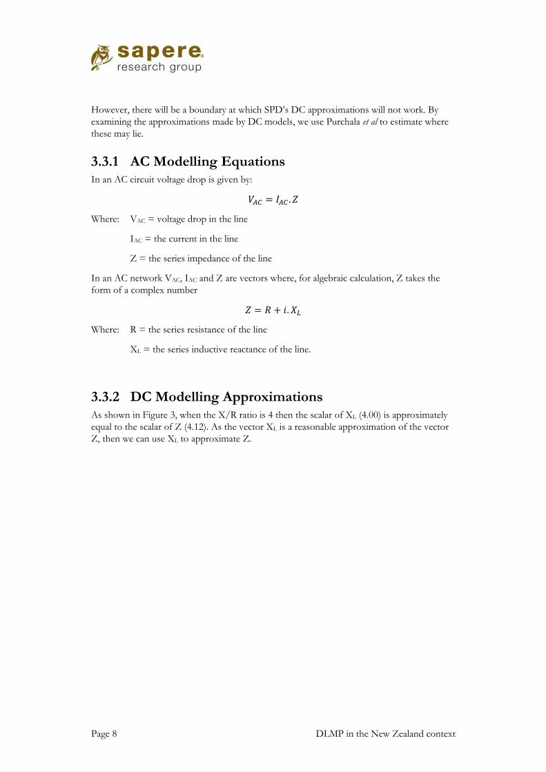
3.3.2 DC Modelling Approximations As shown in Figure 3, when the X/R ratio is 4 then the scalar of XL (4.00) is approximately
equal to the scalar of Z (4.12). As the vector XL is a reasonable approximation of the vector
Z, then we can use XL to approximate Z.
DLMP in the New Zealand context Page 9
Figure 3 - Vectorised representation of Z with an X/R ratio of 4
As XL has no resistance, and if we ignore resistance in any subsequent power flow analysis,
then it can be treated as a real number rather than a complex number. Therefore, it can be
substituted in the place of R in the DC formula for voltage drop (V=I.R), giving:
𝑉𝐷𝐶 = 𝐼𝐷𝐶 . 𝑋𝐿
This is the DC approximation to the “true” AC characteristic.
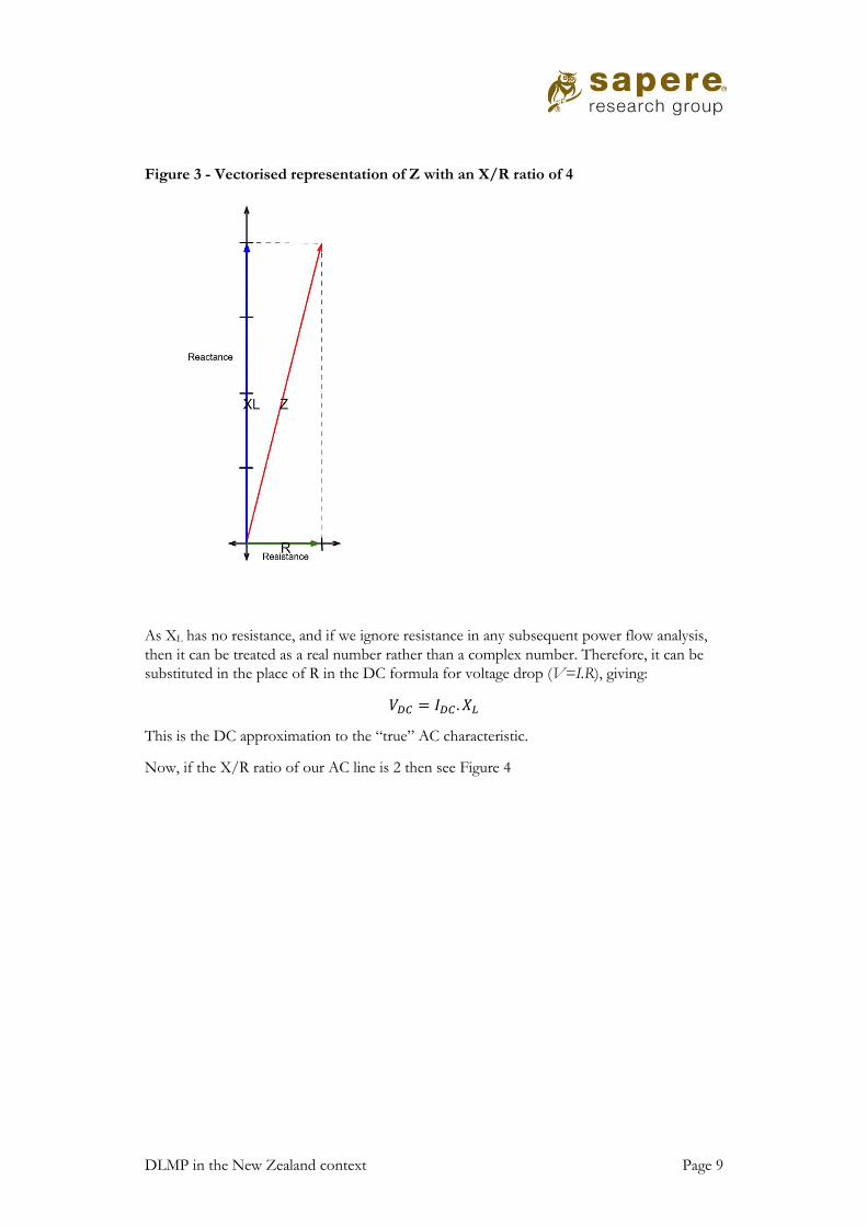
Now, if the X/R ratio of our AC line is 2 then see Figure 4
Page 10 DLMP in the New Zealand context
Figure 4 - Vectorised representation of Z with an X/R ratio of 2
Now the scalar of XL (2.00) is becoming more different from the scalar of Z (2.24). As well
the vector XL is no longer a reasonable approximation of the vector Z. Substituting XL for R
in a DC approximation will now yield a greater error.
In short lines, as both XL and R is low, then voltage drop will be low and errors will be
insignificant. In some ways, the variability of voltage profile is a better indicator of suitability
for standard DC approximations, and their use in deriving LMP prices. Purchala (2005)
concluded that the errors in a DC approximation were the most sensitive to variance in the
voltage profile. As stated above, Purchala et al submitted that “Flat voltage profile means that the
standard deviation of voltages SU < 0.01”. However, as discussed above, SPD is a more advanced
DC load flow model than the one tested in Purchala (2005) and so may be accurate with a
greater range of voltages levels.
However, the voltage range applies to the whole network that is modelled. Hence, if the
voltage distribution around the current SPD network is already near the limit for accurate
modelling by SPD13, then it is likely that very few nodes susceptible to voltage drop could be
added to the existing formulation without compromising accuracy. This is a piece of
investigation that should be carried out early in the assessment of adding new networks to
SPD.
We have insufficient data to establish the standard deviation of voltage in the network
modelled by SPD and cannot directly compare SPD to the literature. Therefore, we cannot
form any firm conclusions about how much deeper the current modelling approach could be
pushed below the level of existing GXPs. To make approximations for the purpose of this
13 We cannot at this point give any guidance on whether this is the case. Transpower should be able to advise the
degree to which the DC approximations around the network are within an acceptable appetite for error.
DLMP in the New Zealand context Page 11
paper we rely firstly on the X/R ratio and then the typical voltage drop in the context of
particular parts of the non-Transpower network and its various characteristics.
3.4 Identifying transmission nodes and lines We expect that all current nodes and lines modelled in SPD satisfy our definition of
transmission in Section 3. The fact that there is a causal relationship between high operating
voltage and high X/R14 raises the question of whether the technical boundary of the
transmission system is beyond the current set of GXPs. Purchala (2005) assessed X/R ratios
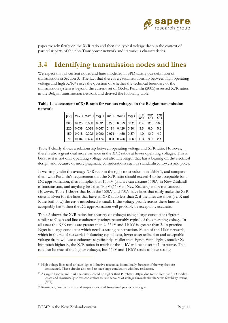
in the Belgian transmission network and derived the following table.
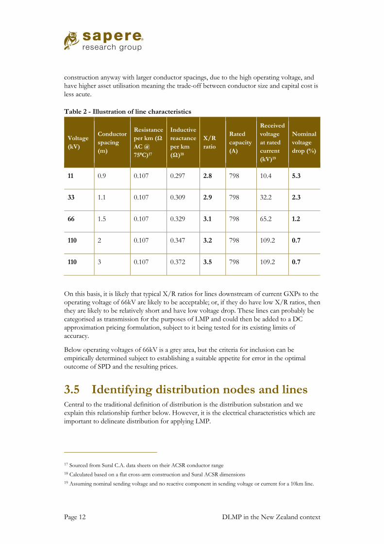
Table 1 - assessment of X/R ratio for various voltages in the Belgian transmission
network
Table 1 clearly shows a relationship between operating voltage and X/R ratio. However,
there is also a great deal more variance in the X/R ratios at lower operating voltages. This is
because it is not only operating voltage but also line length that has a bearing on the electrical
design, and because of more pragmatic considerations such as standardised towers and poles.
If we simply take the average X/R ratio in the right-most column in Table 1, and compare
them with Purchala’s requirement that the X/R ratio should exceed 4 to be acceptable for a
DC approximation, then it implies that 150kV (and we can assume 110kV in New Zealand)
is transmission, and anything less than 70kV (66kV in New Zealand) is not transmission.
However, Table 1 shows that both the 150kV and 70kV have lines that easily make the X/R
criteria. Even for the lines that have an X/R ratio less than 2, if the lines are short (i.e. X and
R are both low) the error introduced is small. If the voltage profile across these lines is
acceptably flat15, then the DC approximation will probably be acceptably accurate.
Table 2 shows the X/R ratios for a variety of voltages using a large conductor (Egret16 –
similar to Goat) and line conductor spacings reasonably typical of the operating voltage. In
all cases the X/R ratios are greater than 2. 66kV and 110kV is greater than 3. In practice
Egret is a large conductor which needs a strong construction. Much of the 11kV network,
which in the radial network is balancing capital cost, lower asset utilisation and acceptable
voltage drop, will use conductors significantly smaller than Egret. With slightly smaller XL
but much higher R, the X/R ratios in much of the 11kV will be closer to 1, or worse. This
can also be true of the higher voltages, but 66kV and 110kV tends to have strong
14 High voltage lines tend to have higher inductive reactance, intentionally, because of the way they are
constructed. These circuits also tend to have large conductors with low resistance.
15 As argued above, we think the criteria could be higher than Purchala’s .01pu, due to the fact that SPD models
losses and dynamically solves constraints to take account of voltage through simultaneous feasibility testing
(SFT)
16 Resistance, conductor size and ampacity sourced from Sural product catalogue
Page 12 DLMP in the New Zealand context
construction anyway with larger conductor spacings, due to the high operating voltage, and
have higher asset utilisation meaning the trade-off between conductor size and capital cost is
less acute.
Table 2 - Illustration of line characteristics
Voltage
(kV)
Conductor
spacing
(m)
Resistance
per km (Ω
AC @
75⁰C)17
Inductive
reactance
per km
(Ω)18
X/R
ratio
Rated
capacity
(A)
Received
voltage
at rated
current
(kV)19
Nominal
voltage
drop (%)
11 0.9 0.107 0.297 2.8 798 10.4 5.3
33 1.1 0.107 0.309 2.9 798 32.2 2.3
66 1.5 0.107 0.329 3.1 798 65.2 1.2
110 2 0.107 0.347 3.2 798 109.2 0.7
110 3 0.107 0.372 3.5 798 109.2 0.7
On this basis, it is likely that typical X/R ratios for lines downstream of current GXPs to the
operating voltage of 66kV are likely to be acceptable; or, if they do have low X/R ratios, then
they are likely to be relatively short and have low voltage drop. These lines can probably be
categorised as transmission for the purposes of LMP and could then be added to a DC
approximation pricing formulation, subject to it being tested for its existing limits of
accuracy.
Below operating voltages of 66kV is a grey area, but the criteria for inclusion can be
empirically determined subject to establishing a suitable appetite for error in the optimal
outcome of SPD and the resulting prices.
3.5 Identifying distribution nodes and lines Central to the traditional definition of distribution is the distribution substation and we
explain this relationship further below. However, it is the electrical characteristics which are
important to delineate distribution for applying LMP.
17 Sourced from Sural C.A. data sheets on their ACSR conductor range
18 Calculated based on a flat cross-arm construction and Sural ACSR dimensions
19 Assuming nominal sending voltage and no reactive component in sending voltage or current for a 10km line.
DLMP in the New Zealand context Page 13
3.5.1 Distribution substation The distribution substation is the last substation before the ICP. Generally, but not always,
the distribution substation will supply a LV network.
3.5.2 Secondary distribution network The secondary distribution network is the network downstream of the distribution
substation and is the network that supplies consumer installations. It is usually Low Voltage
(230/400V in New Zealand).
Typical X/R ratios for low voltage overhead lines are around 1. LV networks also feature
high amounts of underground cabling where X/R ratios can be significantly less than 1.
The LV network is very low voltage. The statutory voltage drop limit of 6% (technically, a
variance of ±6% ) is only ±14 volts for a single-phase 230V supply. In practice distributors
try to manage voltage so that the lightly loaded voltage output from distribution substations
is high. This allows them to tolerate more than 14V of drop and maintain voltage within
statutory limits. Many low voltage circuits are managed to use the whole ±6% range. The
voltage of any installation on such circuits depends on the distance from the substation. It is
relatively straightforward to conclude, therefore, that the voltage profile around the LV
network will be far from flat, but also that the primary job of distribution management is the
management of voltage (to remain within statutory limits).
We are confident in saying that LV networks, and secondary distribution networks generally,
will not meet the requirements of a DC approximation to power flow. They would require
AC modelling techniques to correctly represent power flow, losses and congestion.
3.5.3 Primary distribution network The network that operates downstream of transmission or zone substations and supplies the
distribution substations is the primary distribution network. The primary side of distribution
substations is usually, but not always, 11kV.
Most 11kV is probably overhead but there can be long lengths of cable. Radial circuits tend
to have relatively small conductors (balancing a fine line between low utilisation and voltage
drop) and resistance is high. The 11kV lines near zone substations can have large conductors
with low resistance but similar construction and similar reactance, and a high X/R ratio.
Overall, most 11kV probably has a X/R ratio of greater than 1 but less than 2.
Most 11kV is radial and relatively long. Generally, the 11kV network is managed to a voltage
profile integrated with the voltage profile of the LV network. Overall, we suspect that the
11kV network, and the primary distribution network generally, will not meet the criteria for
DC approximation.
3.5.4 Zone substation A zone substation is any substation that is downstream of a GXP but upstream of a
distribution substation. Generally, in New Zealand, there will be one zone substation
between the GXP and distribution substation but there is often none and may occasionally
be two.
Page 14 DLMP in the New Zealand context
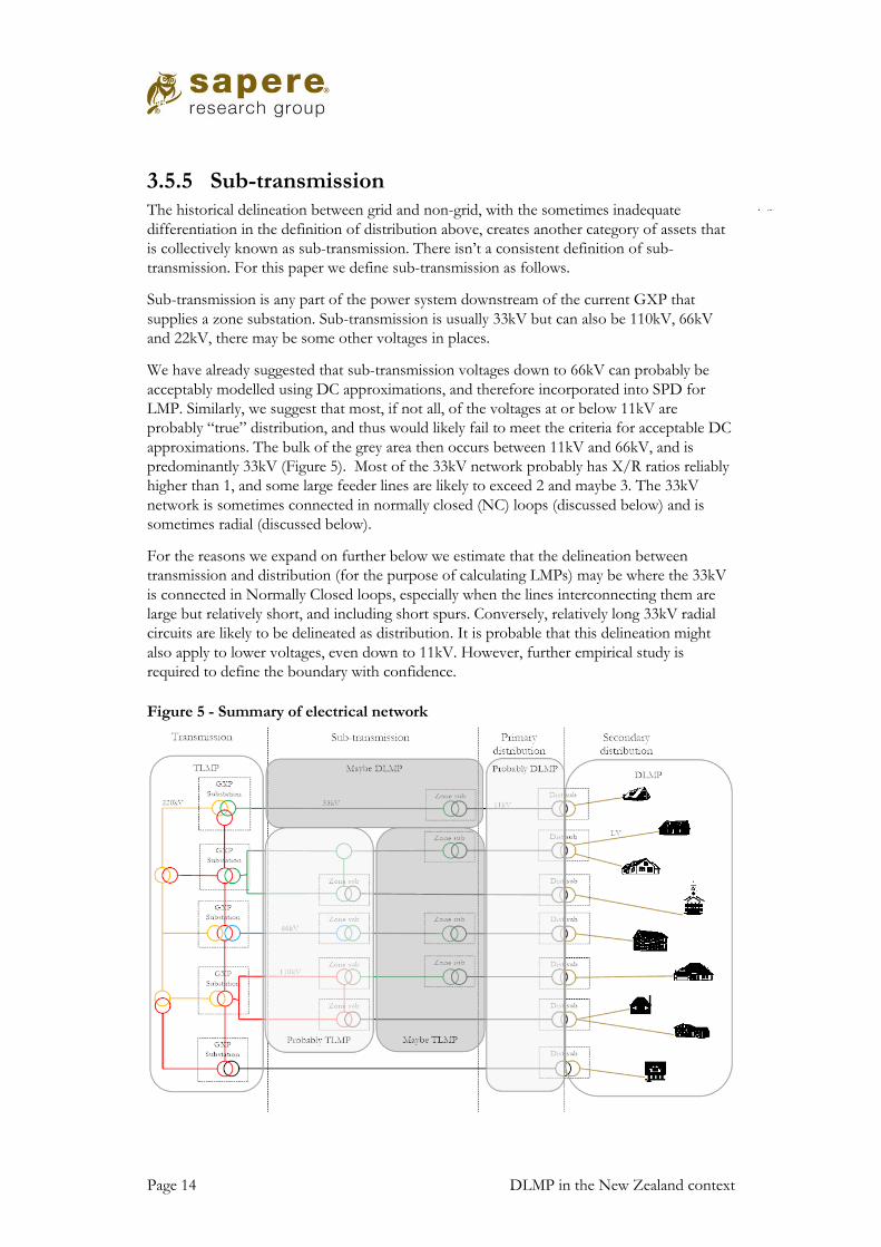
3.5.5 Sub-transmission The historical delineation between grid and non-grid, with the sometimes inadequate
differentiation in the definition of distribution above, creates another category of assets that
is collectively known as sub-transmission. There isn’t a consistent definition of sub-
transmission. For this paper we define sub-transmission as follows.
Sub-transmission is any part of the power system downstream of the current GXP that
supplies a zone substation. Sub-transmission is usually 33kV but can also be 110kV, 66kV
and 22kV, there may be some other voltages in places.
We have already suggested that sub-transmission voltages down to 66kV can probably be
acceptably modelled using DC approximations, and therefore incorporated into SPD for
LMP. Similarly, we suggest that most, if not all, of the voltages at or below 11kV are
probably “true” distribution, and thus would likely fail to meet the criteria for acceptable DC
approximations. The bulk of the grey area then occurs between 11kV and 66kV, and is
predominantly 33kV (Figure 5). Most of the 33kV network probably has X/R ratios reliably
higher than 1, and some large feeder lines are likely to exceed 2 and maybe 3. The 33kV
network is sometimes connected in normally closed (NC) loops (discussed below) and is
sometimes radial (discussed below).
For the reasons we expand on further below we estimate that the delineation between
transmission and distribution (for the purpose of calculating LMPs) may be where the 33kV
is connected in Normally Closed loops, especially when the lines interconnecting them are
large but relatively short, and including short spurs. Conversely, relatively long 33kV radial
circuits are likely to be delineated as distribution. It is probable that this delineation might
also apply to lower voltages, even down to 11kV. However, further empirical study is
required to define the boundary with confidence.
Figure 5 - Summary of electrical network
DLMP in the New Zealand context Page 15
3.6 Loop, mesh and radial
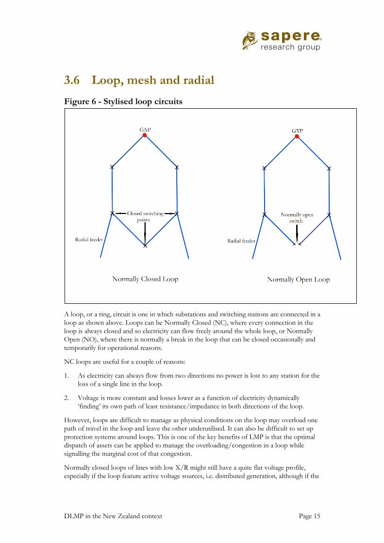
Figure 6 - Stylised loop circuits
A loop, or a ring, circuit is one in which substations and switching stations are connected in a
loop as shown above. Loops can be Normally Closed (NC), where every connection in the
loop is always closed and so electricity can flow freely around the whole loop, or Normally
Open (NO), where there is normally a break in the loop that can be closed occasionally and
temporarily for operational reasons.
NC loops are useful for a couple of reasons:
1. As electricity can always flow from two directions no power is lost to any station for the
loss of a single line in the loop.
2. Voltage is more constant and losses lower as a function of electricity dynamically
‘finding’ its own path of least resistance/impedance in both directions of the loop.
However, loops are difficult to manage as physical conditions on the loop may overload one
path of travel in the loop and leave the other underutilised. It can also be difficult to set up
protection systems around loops. This is one of the key benefits of LMP is that the optimal
dispatch of assets can be applied to manage the overloading/congestion in a loop while
signalling the marginal cost of that congestion.
Normally closed loops of lines with low X/R might still have a quite flat voltage profile,
especially if the loop feature active voltage sources, i.e. distributed generation, although if the
Page 16 DLMP in the New Zealand context
generation is intermittent it might exacerbate the range of voltages in the profile. The effect
of connecting lines in parallel is that the equivalent impedance at the parallel point is less
than in both lines. Therefore, relatively longer loops can have impedance that is low enough
not to introduce significant error for DC approximation, compared to a radial circuit.
In distribution networks the management of loops is currently made difficult due to the lack
of dispatchable assets, or it is prohibitively expensive to manage NC loops, and so the more
common form of loop, particularly below sub-transmission, is NO.
NO loops are quite common in distribution and allow for the backup supply of areas from
other feeders during outages or for other operational reasons. Usually, though, the
conversion of NO loops into NC loops is made temporarily and only for short durations.
Therefore, for the purposes of discussing how to practically implement DLMP we are going
to treat NO loops as radial circuits. Although, we must be cognisant that parts of the
distribution network can switch between radial feeders.
A meshed network is one where substations and switching stations are connected to multiple
other stations through multiple lines – i.e., loops exist. In a mesh network, multiple loops can
make the operation and dispatch of meshed networks very complicated. Again, this is one of
the key benefits arising from optimised load flow models, which then also produce marginal
prices at each node of the meshed network.
While much of the transmission network is meshed, meshes are much less common in the
distribution network.
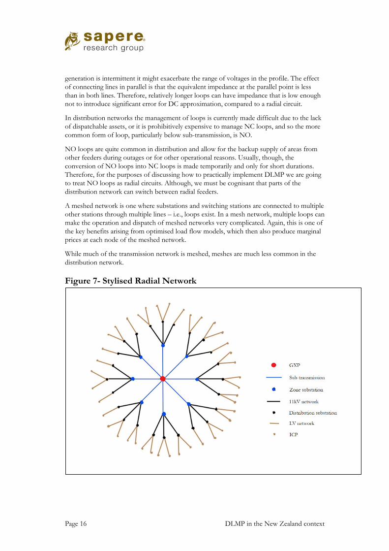
Figure 7- Stylised Radial Network

DLMP in the New Zealand context Page 17
Radial feeders ‘radiate’ out from a single point of supply as in the diagram above. In a radial
network, there are no NC loops and every point in the radial network is completely
dependent on the single upstream path for supply. Most of the distribution network,
especially below sub-transmission, is radial but NO loops are also common; which, as
discussed above, we are still treating as fundamentally radial for the purposes of DLMP.
Page 18 DLMP in the New Zealand context
4. Distribution – Depth, Granularity and Definition of Nodes/Zones
The depth of LMP coverage into the distribution network has a significant impact on
shaping the available options for LMP. For example, if the objective is to provide LMP
down to individual installations then many model approaches are currently impractical, and
the level and density of network information required by these models may not be practically
available. However, if the objective is to implement a highly accurate modelling approach to
the level of the 33kV network, for example, then granularity is restricted in the sense that
many installations at differing locations in the network below 33kV will have the same
locational marginal price.
Also, while limiting depth necessarily limits granularity (i.e., ICP-based granularity does not
make sense in a 33kV model), the reverse doesn’t apply (e.g., the optimisation could apply
down to the LV network, but prices could be “rolled up” into zones via clustering).
The depth question is also relevant to the question of whether the pricing models are single
models or hybrids. For example, it is probably practical to extend TLMP pricing into some
of the sub-transmission network, but DC approximations won’t work for all radial networks.
A deeper approach to LMP could still be pursued by using hybrid of a DC approximation
for the appropriate parts, and a simplified AC approximation approach for the radial
network where DC approximations are not suitable.
DLMP in the New Zealand context Page 19
Figure 8 - Zone substation node and implied zone
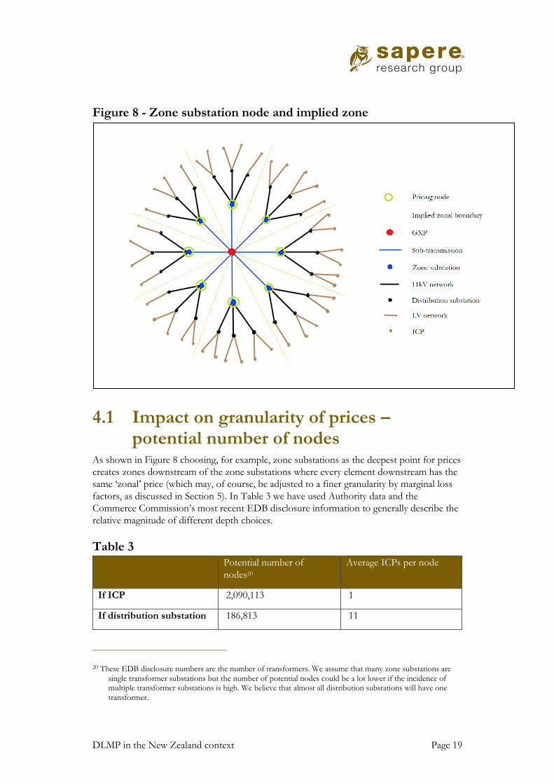
4.1 Impact on granularity of prices – potential number of nodes
As shown in Figure 8 choosing, for example, zone substations as the deepest point for prices
creates zones downstream of the zone substations where every element downstream has the
same ‘zonal’ price (which may, of course, be adjusted to a finer granularity by marginal loss
factors, as discussed in Section 5). In Table 3 we have used Authority data and the
Commerce Commission’s most recent EDB disclosure information to generally describe the
relative magnitude of different depth choices.
Table 3
Potential number of
nodes20
Average ICPs per node
If ICP 2,090,113 1
If distribution substation 186,813 11
20 These EDB disclosure numbers are the number of transformers. We assume that many zone substations are
single transformer substations but the number of potential nodes could be a lot lower if the incidence of multiple transformer substations is high. We believe that almost all distribution substations will have one
transformer.
Page 20 DLMP in the New Zealand context
If zone substation 1,261 1,658
If remains GXP 179 11,677
Source: emi.govt.nz, Performance-summaries-for-electricity-distributors.xls (Commerce Commission, May
2017)
A nodal model down to zone substation could create approximately 1,200 new nodes, where
each new nodal price would effectively become a zonal price for around 1,600 ICPs on
average21.
Similarly pushing a nodal model down to the distribution substation level would create
187,000 new nodal prices, where each new node would effectively become a zonal price for
11 ICPs on average22.
Figure 9 - ICP nodal pricing with zone aggregation
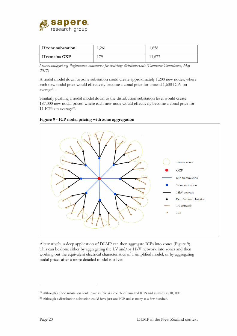
Alternatively, a deep application of DLMP can then aggregate ICPs into zones (Figure 9).
This can be done either by aggregating the LV and/or 11kV network into zones and then
working out the equivalent electrical characteristics of a simplified model, or by aggregating
nodal prices after a more detailed model is solved.
21 Although a zone substation could have as few as a couple of hundred ICPs and as many as 10,000+
22 Although a distribution substation could have just one ICP and as many as a few hundred.
DLMP in the New Zealand context Page 21
In both cases it would be counterproductive to group nodes into zones that had quite
different electrical characteristics. Therefore, the electrical network will constrain the choice
of zones to some extent.
Granularity does not constrain depth in practice as the granularity discussion is
fundamentally about whether we want to constrain the number of prices for reasons of
workability and practicality. However, there may be reasons why the ICP, for example, is
chosen as an ideal place in the network to differentiate on the basis of DLMP. The
consequence of this choice is then to constrain granularity to 2 million nodes and the depth
to ICP level.
The choice then between the dimensions of depth, granularity and definition of node/zone
is a choice between the level of differentiation to be signalled through the network, the
number of prices that results and the net benefits of signalling LMP to a specific location,
e.g. ICP. However, these choices are also interrelated with choices of governance, the
definition of DSO and modelling approaches.
4.2 Assessment required to determine suitability of DC approximation
To build and operate any LMP model would require the electrical characteristics of any line
or substation added to the model to have current information to the correct level of detail
and telemetry to allow operation and monitoring of key variables that are inputs into the
process for formulating prices. Pricing nodes would also, ideally, have TOU metering for
settlement, although volumes could be derived from the aggregation of existing ICP
metering.
We haven’t made a survey of the status of distribution networks in this regard but we have
made the following assumptions. As discussed above NC loops are difficult to manage and
zone substations are important potential nodes in the sense that they affect large numbers of
customers. It is our expectation that all sub-transmission mesh will be actively managed by
the lines companies and the requisite information and telemetry will exist. There is likely to
be many zone substations on radial feeders that also meet the requirements.
However, some zone substations will be of a size and scale little larger than distribution
substations and so we assume that not all zone substations will meet the requirements.
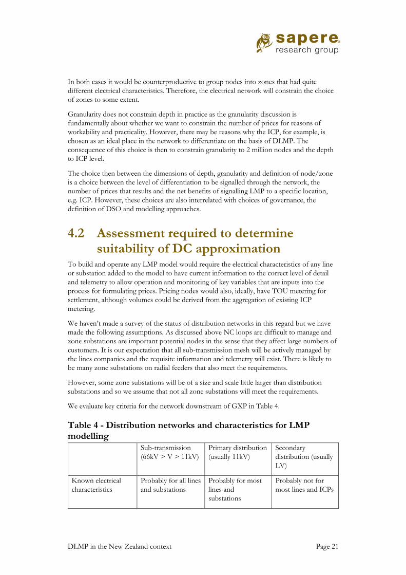
We evaluate key criteria for the network downstream of GXP in Table 4.
Table 4 - Distribution networks and characteristics for LMP modelling
Sub-transmission
(66kV > V > 11kV)
Primary distribution
(usually 11kV)
Secondary
distribution (usually
LV)
Known electrical
characteristics
Probably for all lines
and substations
Probably for most
lines and
substations
Probably not for
most lines and ICPs
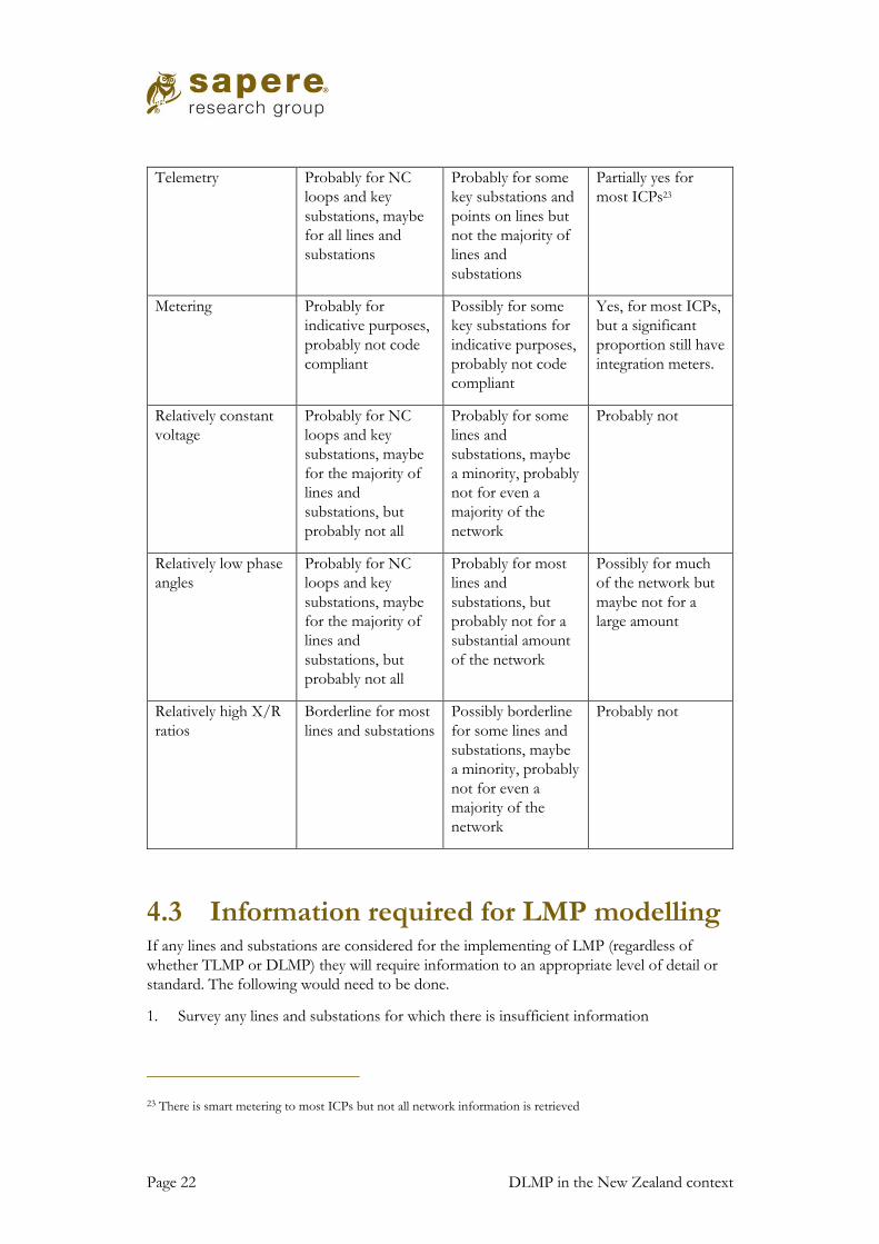
Page 22 DLMP in the New Zealand context
Telemetry Probably for NC
loops and key
substations, maybe
for all lines and
substations
Probably for some
key substations and
points on lines but
not the majority of
lines and
substations
Partially yes for
most ICPs23
Metering Probably for
indicative purposes,
probably not code
compliant
Possibly for some
key substations for
indicative purposes,
probably not code
compliant
Yes, for most ICPs,
but a significant
proportion still have
integration meters.
Relatively constant
voltage
Probably for NC
loops and key
substations, maybe
for the majority of
lines and
substations, but
probably not all
Probably for some
lines and
substations, maybe
a minority, probably
not for even a
majority of the
network
Probably not
Relatively low phase
angles
Probably for NC
loops and key
substations, maybe
for the majority of
lines and
substations, but
probably not all
Probably for most
lines and
substations, but
probably not for a
substantial amount
of the network
Possibly for much
of the network but
maybe not for a
large amount
Relatively high X/R
ratios
Borderline for most
lines and substations
Possibly borderline
for some lines and
substations, maybe
a minority, probably
not for even a
majority of the
network
Probably not
4.3 Information required for LMP modelling If any lines and substations are considered for the implementing of LMP (regardless of
whether TLMP or DLMP) they will require information to an appropriate level of detail or
standard. The following would need to be done.
1. Survey any lines and substations for which there is insufficient information
23 There is smart metering to most ICPs but not all network information is retrieved
DLMP in the New Zealand context Page 23
2. Install all required telemetry where it doesn’t currently exist
3. Install code compliant metering or establish an alternative that is acceptable for
settlement
This part of the network has up to an order of magnitude more nodes than the current SPD
specification (~1,600 vs 179, as per Table 3).
However, for the purposes of an optimal power flow (OPF) model, the scale of the problem
increases substantially by more than two orders of magnitude.
The line and substation surveys would not only be two orders of magnitude larger but there
would be far less homogeneity about the types of 11kV and distribution substation
construction with many more configurations.
To meet the same standards as current GXPs then telemetry would need to be retrofitted to
most distribution substations and code compliant revenue metering to just about all of them.
For many, and maybe most, distribution substations retrofitting telemetry and, especially,
metering would be infeasible without substantially modifying the substations.
To push into the LV network would also make the scale of the OPF approach greater than
an order of magnitude again. In addition to the same surveying problems as the 11kV, the
LV network would have an even greater composition of underground, or otherwise hidden,
cabling.
However, the telemetry requirements are partially solved and the metering requirements are
there for 75% of the ICPs. Smart meters can obviously be used now for half-hourly
settlement and could be set up for real-time pricing (down to 1 minute periods). They meter
active power, reactive power, apparent power, voltage, current, frequency, Total Harmonic
Distortion and voltage sag/swell events; and, therefore, they could be used for operational
telemetry. However, we understand that most data are not currently available and they
probably cannot be polled fast enough, currently, to meet the same standards as GXPs,
although GXP level telemetry need not be the required standard for a DLMP solution.
Targeted approaches, where feeders are added depending on the net benefits of applying
DLMP to feeders with increasing levels of DER, would be more easily achievable and would
suit hybrid modelling approaches.
Simplified modelling approaches would also be more achievable. Simplified equivalent
circuits and zonal price approaches could probably use existing information down to the
distribution substation, at least, and could probably be approximated for the LV network as
well.
Page 24 DLMP in the New Zealand context
5. Modelling considerations for calculating DLMP prices
We have established above that the distribution system – beyond sub-transmission - is
sufficiently different from the transmission system that the constant voltage DC
approximation cannot produce robust, efficient prices. In order to produce reliable, efficient
prices to the same standard as TLMP, DLMP must be based on some form of AC model.
5.1 DCOPF models LMP models for the high-voltage grid are reasonably well established now. New Zealand led
the way, being the first country in the world to apply full nodal pricing.
This was done using a DC Optimal Power Flow (DCOPF) model, which we now know as
the Scheduling, Pricing and Dispatch model (SPD). DCOPF models make use of the fact
that, on the transmission network, voltage can be assumed to be constant, and X/R ratios
high, to provide a satisfactory Direct Current (DC) approximation to the (actual) Alternating
Current nature of the system. DCOPF models have the key advantage that the resulting
optimisation problem is linear. Linear (convex) problems can be solved using linear
programs, which have a well-documented range of benefits: principally, that under a range
of conditions they guarantee convergence on a global optimal solution very quickly, and
directly provide optimal nodal prices, since they are the dual variables on the nodal power
flow balance constraint24.
Hence, for those areas of the sub-transmission network where DC approximations are
satisfactory, all the benefits of linear DCOPFs, in terms of marginal pricing (losses and
congestion), are available, irrespective of whether this is achieved as an extension of SPD, or
as a new model which interfaces with SPD at the current GXP boundary.
5.2 Alternative to DCOPF models: ACOPF The more accurate approach to modelling flows on a network, which would be the obvious
candidate in situations where the assumptions of DCOPF models have been rejected, is the
AC (Alternating Current) OPF model.
Ways to “solve” the ACOPF problem abound, but none are without their issues when
considering how to operationalise them for real grids. As far as we are aware, no jurisdiction
is using them for pricing on either transmission or distribution grids.
24 Primal-dual optimality is a key theorem in mathematical programming. Essentially it demonstrates that at the
optimal solution to the quantity problem (“dispatch” in the electricity context), there is an equivalent optimal
solution to the economic problem (“prices” associated with each constraint).
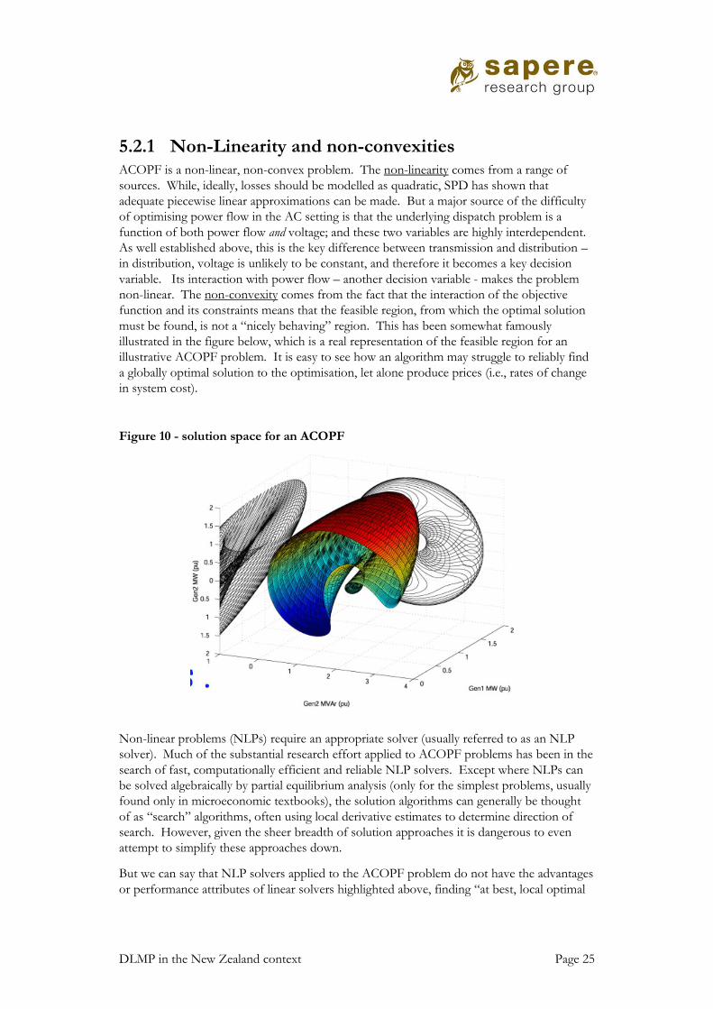
DLMP in the New Zealand context Page 25
5.2.1 Non-Linearity and non-convexities ACOPF is a non-linear, non-convex problem. The non-linearity comes from a range of
sources. While, ideally, losses should be modelled as quadratic, SPD has shown that
adequate piecewise linear approximations can be made. But a major source of the difficulty
of optimising power flow in the AC setting is that the underlying dispatch problem is a
function of both power flow and voltage; and these two variables are highly interdependent.
As well established above, this is the key difference between transmission and distribution –
in distribution, voltage is unlikely to be constant, and therefore it becomes a key decision
variable. Its interaction with power flow – another decision variable - makes the problem
non-linear. The non-convexity comes from the fact that the interaction of the objective
function and its constraints means that the feasible region, from which the optimal solution
must be found, is not a “nicely behaving” region. This has been somewhat famously
illustrated in the figure below, which is a real representation of the feasible region for an
illustrative ACOPF problem. It is easy to see how an algorithm may struggle to reliably find
a globally optimal solution to the optimisation, let alone produce prices (i.e., rates of change
in system cost).
Figure 10 - solution space for an ACOPF
Non-linear problems (NLPs) require an appropriate solver (usually referred to as an NLP
solver). Much of the substantial research effort applied to ACOPF problems has been in the
search of fast, computationally efficient and reliable NLP solvers. Except where NLPs can
be solved algebraically by partial equilibrium analysis (only for the simplest problems, usually
found only in microeconomic textbooks), the solution algorithms can generally be thought
of as “search” algorithms, often using local derivative estimates to determine direction of
search. However, given the sheer breadth of solution approaches it is dangerous to even
attempt to simplify these approaches down.
But we can say that NLP solvers applied to the ACOPF problem do not have the advantages
or performance attributes of linear solvers highlighted above, finding “at best, local optimal
Page 26 DLMP in the New Zealand context
solutions” (O’Neill, 2013). These present potentially significant problems for the generation
of DLMP prices; we note some examples from the academic literature here:
• Murillo-Sanchez et al demonstrated how these solution techniques, in pursuing good
performance, often take large solution steps during their iterative search for the
optimum which struggle when the underlying cost/bid/offer functions are piecewise
linear (an issue for our current market setup). (Murillo-Sanchez and Thomas,
2007). The authors then go on to propose different ways off approximating the
piecewise functions with polynomials or trigonometric functions to avoid this issue. At
the time of writing (2007), these authors noted that there was no robust commercial
AC OPF tool against which they could compare their suggested algorithmic
improvements; they instead use MINOS in MATPOWER as the default
comparator. This counterfactual tool failed to find a solution to the ACOPF problem
in systems exceeding 300 buses, 69 generators and 411 branches.
• More generally, there is some debate over solution times of NLP solvers. Meng and
Chowdhury seem to think on the distribution grid this should solve very fast; Yuan and
Biggar suggest, however, that ACOPF’s in the context of a large number of nodes may
be “computationally intractable” due to non-convexities in the line flow
constraints. Solution times need to be viewed in the context of how rapidly solutions
are required: for Transpower’s 5 minute dispatch needs, a reliable solution is needed
very fast. If hourly prices were required, a slower solution process may be acceptable.
Again, this is an issue which needs to be explored.
• Yuan & Biggar highlight other computational complexities of non-convexities in an
ACOPF. Yuan et al suggest that these can be addressed through applying sequential
tightness algorithms in order to focus the algorithm on the region containing the
optimal solution. They demonstrate this through a 20-bus example.
• However, general experience with some of the best performing semi-definite
programming solvers suggests that, while a close approximation to the primal solution
can be found, the equivalent set of optimal prices can be more problematic. These can
no longer be calculated directly as in the linear programming setting, and rely on
estimation of Lagrangian multipliers25. It is entirely possible that, depending on the
exact nature of the feasible region, a small error in the solution to the primal problem
may lead to large errors in the dual (price) solution. Thus it cannot be always
guaranteed that the resulting nodal prices are the right prices in an auction setting, or
are revenue adequate26.
Despite this, a number of researchers are pursuing promising approaches to LMP in the
context of ACOPF models (e.g., Yuan and Biggar). Richard O’Neill (Chief Economic
Advisor for Federal Electric Reliability Council in the US) is probably one of the most active
25 Lagrangian multipliers can be thought of as the partial derivative of total cost with respect to a particular
constraint. The figure above should make it relatively clear how erroneous such an estimate could be, even if something close to the optimum is found.
26 We are aware informally that there has been a significant debate at FERC, over a number of years, around what
the correct prices are for some implementations of DCOPF in the US setting. These problems become non-convex due to the inclusion of integer variables representing unit commitment decisions; hence the pricing models are not linear programs like NZ, but Mixed Integer Programs.
DLMP in the New Zealand context Page 27
researchers in this space27. We note that, however, based on the literature we have observed,
the test problems remain small (usually <20 nodes). In any case, an ACOPF model would
need to be subjected to rigorous testing to meet a “dispatch” standard. This is an area which
would require investigation.
5.2.2 Modelling constraints for congestion prices If congestion were to be modelled, there are a number of options:
• Simple thermal constraints (ratings on individual lines) would be appropriate for radial
networks and could relatively easily be incorporated into either a DC or AC OPF. This
would require information on the ratings of the lines (and transformers) in question, as
discussed in Section 4.
• Group security constraints (where multiple paths exist in meshed networks) may be
more appropriate at higher distribution voltages, depending on network topology. Until
the development of Simultaneous Feasibility Testing (SFT), Transpower developed
these constraints for the grid manually. A manual approach may still be appropriate for
networks if the degree of “meshing” is small, and only a small number of security
constraints need to be developed.
• Voltage constraints may possibly be the area where the most development is required.
They are relevant to both radial and meshed networks. In a working ACOPF model,
voltage constraints are naturally incorporated. In a DCOPF model, voltage constraints
have to be developed offline and entered into the DCOPF model as a restriction on
active power flow (in much the same way as Transpower uses SFT and its Voltage
Stability Assessment Tool, VSAT, although SFT is more dynamically integrated with the
SPD solution process). While offline tools may work for a small number of group
security constraints, it is likely to be unworkable for a distribution network with voltage
deviations across the network (which would require a high number of constraints, the
right-hand side of the constraints to be constantly amended). Again, however, this
depends on the depth of the DLMP approach; for some networks, pricing at the 33kV
level may only require voltage constraints to be developed for a small number of nodes.
This is ultimately an empirical question related to depth and the nature of the network.
• Constraints for other aspects of power quality may be relevant – e.g., frequency. There
is no international literature on developing security constraints in an ACOPF setting for
these aspects of the power system.
• A form of congestion pricing could also be applied using smart metering information as
the meters could measure capacity, voltage and power quality levels within operating
envelopes, i.e. exceeding the operating envelopes could result in marginal consumption
being priced at an administered congestion price.
27 Dick O’Neill’s 2013 presentation on ACOPF models suggested that the Linear IV formulation of the ACOPF
model, which has linear constraints and a quadratic objective function, looks promising in the context of the American MIP approach to pricing. As NZ does not currently incorporate unit commitment variables in
SPD< this could be even more promising for us.
Page 28 DLMP in the New Zealand context
However, when considering any type of flow constraint, note the caution above about the
accuracy of models; poorer performance in terms of estimating line flows will result in much
lower confidence that any congestion signal is “efficient”.
5.2.3 Summary – Modelling Options From a modelling perspective, therefore, there are four broad options:
(i) LMP is only extended into those areas of the sub-transmission network which satisfy the requirements of a DCOPF. This could be done either as an extension to SPD, or through models built by distribution system operators that interface with SPD at the GXP.
(ii) DLMP is provided by extending the System Operator’s SPD model (converted into an ACOPF) into the “true” distribution grid (at some depth), and/or
(iii) DLMP is provided using a disaggregated approach, where SPD remains approximately as it is (possibly widening its definition of the “grid edge” by including distribution-voltage nodes which connect current GXPs in parallel), and DLMP further into the distribution network is potentially provided by separate ACOPF models (developed by either the TSO or DSOs) which take the GXP price and produce DLMP
(iv) Option (i) plus the use of AC approximations to marginal losses, and/or administered congestion pricing using smart metering information
While option (i) has some significant complexity in terms of information sharing between
numerous different asset owners, from a modelling perspective it does not seem
problematic.
As “true” DLMP requires an AC model, approach (ii) would require SPD to become an
ACOPF model. While, in time, reliable solutions to ACOPF models are likely to emerge, at
this point in time this would not be practical. If SPD was to be changed to an ACOPF
model, it may become large enough to cause concern over computational complexity. Again,
this would depend on the depth of the model; if it was extended across NZ to zone
substations, the revised SPD model would have ~1,400 nodes, about half the level Murillo-
Sanchez found would cause MATPOWER to fail, but well in excess of the largest test they
conducted which found an optimum (300 nodes). This would be a necessary avenue of
investigation for more confidence.
With a disaggregated approach (iii), SPD could be left as a linear model, and the DLMPs
could be produced by ACOPF models which only covered the distribution grid and only
interfaced with SPD via the GXP price. If done on an individual network approach, the
largest network (Vector) would require 214 nodes if modelled to the zone substation level,
which may be more manageable28. But we reinforce our concerns about the reliability of
prices from ACOPF models.
28 There is some concern expressed in the literature that, depending on the nature of the individual models, the
functions passed between them, and the sequential/iterative approaches finding optima, overall unique global solutions may not be found, and, in some situations, that multiple solutions might be found (a problem known as “degeneracy”). LP optimisation for DER aggregator doesn’t work in some situations.
DLMP in the New Zealand context Page 29
Very few authors have considered how the DSO and TSO would interact in this case. This
is an issue with the hybrid approach irrespective of whether the DSO and TSO are the same
entity or not29. Yuan et al suggested generalised bid functions be used to represent the
behaviour of DER as a function of grid price. We believe this is a fruitful avenue of
research.
Regarding option (iv) the higher level of losses experienced in the distribution network (see
Section 3.3) has led a number of authors to focus solely on incorporating losses into the
DLMP price (and ignore congestion) e.g., Shaloudegi30, Sotkiewicz31. This is done by simply
taking a grid price and adjusting it by a marginal loss factor (i.e., the partial derivative of
losses with respect to current).
The focus on losses also seems to be driven by a view that, especially in radial networks,
congestion is unlikely to be a problem (Shaloudegi), as lines will have been built in a context
of one-way flow to completely supply demand at the end of the line. The implicit
assumption is that DER will only further support the capacity on these lines, and hence
congestion is even less likely to be an issue. However, this appears naïve, if for no other
reason than growth and its impact on the shallower (MV) part of the network, as well as the
question of reinvestment with respect to ageing assets. That said, it would provide prices
that are closer to the efficient ideal than is currently the case in NZ.
However, we note that the application of marginal loss factors to the GXP price (and
ignoring constraints) has some merit:
• To some extent, the status quo in New Zealand could be thought of as DLAP
(distribution locational average pricing) since that, effectively, the price at the local
“zone” is actually the GXP price adjusted by average network loss factors (which are
governed by the Code).
• These average loss factors are re-estimated by network companies relatively
infrequently. Hence a (conceptually) simple extension to the status quo would be to
require network companies to re-estimate these factors as marginal loss factors, and re-
estimate or calibrate them more frequently or on a greater granularity (e.g.,
WDODDN). This could provide half-hourly prices to the “zone” albeit with averaged
marginal loss factors.
• While conceptually simple, estimating marginal loss factors may not be trivial. While
annual average total losses can be estimated from historical annual metered quantities,
(e.g., EV charging) unless can anticipate how DLMP will change for a change in charging policy
(degeneracy). General problem with iterative methods as they can get caught on steps of the supply function
29 If they were indeed the same entity, this would simply make the issue of information exchange simpler.
However, the problem of how to incorporate the optimal behaviour of DER in an ACOPF model, into a DCOPF model, remains.
30 K. Shaloudegi, N. Madinehi, S. H. Hosseinian, and H. A. Abyaneh (2012), “A novel policy for locational
marginal price calculation in distribution systems based on loss reduction allocation using game theory,” IEEE
Trans. Power Syst., vol. 27, no. 2, pp. 811–820, May 2012.
31 Sotkiewicz, P. M. and J. M. Vignolo (2006). "Nodal pricing for distribution networks: Efficient pricing for
efficiency enhancing DG." IEEE Transactions on Power Systems 21(2): 1013-1014.
Page 30 DLMP in the New Zealand context
even annual average marginal losses cannot be done in the same way32. To do it
accurately requires the total losses between the GXP and the node or zone to be
estimated (using a power flow model) or metered (if using historical quantities) at a
reasonably fine time resolution, before averaging up to the desired resolution.
However, we expect that, at some depths, historical information on half-hourly or
hourly metered quantities should be available for most networks. As discussed
previously, with smart meters, with a suitably comprehensive analytical approach, it
could possibly be done right down to the ICP level on radial networks.
Hence, as an intermediate step towards full loss and congestion pricing, an ex-post (or real-
time) marginal loss factor pricing approach could be more easily developed that does not
require full ACOPF optimisation models to be developed. While this may seem a very small
step towards proper DLMP (losses and congestion with optimal dispatch), the relatively
higher level of losses on the distribution network will still provide a locational signal.
We reinforce though, that – if the historical averaging approach is taken – these prices will
not be “optimal” in any given period. This will especially be true if the resulting loss-based
DLMP prices instigate a response (e.g., installation of DER), which will not be picked up by
the averaging until the next calibration (which could include real-time calibration, but not
forward-looking).
Finally, we highlight an issue picked up below: by moving to marginal losses on the
distribution network (as with constraints) a settlement surplus will be created.
5.2.4 Bidding, Offering and Prices DLMP signals only matter (from an incentive perspective) if they are the prices that are used
for payment (clearing, settlement, and reconciliation). Hence demand bids and generation
offers (where relevant33) would be made at the DXP. Under the current dispatch process,
demand forecasts at the DXP would also have to be formed or sourced by the entity solving
the AC or DC dispatch model. Note that this implies changes to the systems and processes
for purchasers (and potentially generators where they are connected to a DXP).
We have not been asked to speculate on the prices that could arise with a DLMP approach.
However, from a practicality perspective, we make the following observations:
• As discussed above, settlement using marginal pricing leads to a settlement surplus.
Settlement surpluses on the grid are dealt with using a Code-based process, although we
note that there has been significant historical debate about to whom the settlement
surplus should rightly accrue. An approach would have to be developed for the
distribution surplus, which could include recycling it back to distribution companies to
offset network costs.
32 The problem is that, while marginal losses (2IR) at a point in time are twice average losses (IR), once losses are
averaged through time, this relationship falls down due to the non-linearity of total losses. That is, average marginal losses through time is not equal to the marginal loss of average losses through time. Simple examples can be constructed to demonstrate this. Hence, better approximations would need to be found by modelling marginal losses on a daily or hourly basis, and then averaged to get a monthly, seasonal, and/or
WDODDN pattern.
33 The majority of current generation plant is connected at the GXP, hence would continue to offer at the GXP.
DLMP in the New Zealand context Page 31
• We make the (obvious) observation that moving from the current average-loss based
pricing approach to marginal losses for settlement will instantly result in an increase in
purchase costs (which would presumably be passed on to customers). This needs to be
considered along with the use of the settlement surplus.
• We presume that DLMP is used for clearing and settlement in the same way as grid
LMP, i.e., they are simply used by purchasers to settle purchase costs. Whether this
resulted in the retailers passing through the “signals” on a zone-by-zone level is an open
question. So the Authority may consider how these prices are “published” in a way
which has the intended effect.
• The default assumption thus far is that DLMP would be applied on the chosen
granularity/depth irrespective of whether there are responsive DER in those parts of
the network34. However, we note that, in this respect, the distribution network is (in its
current state) quite different to the grid. In most parts of the high-voltage grid, there
are discretionary/dispatchable generators on both sides of any individual transmission
constraint. This is not currently the case for the distribution grid. Hence, in applying
constraints to a network without reference to the number of dispatchable or
discretionary DERs, a binding constraint may just result in an infeasibility (under the
current approach to scarcity) or – using the Authority’s proposed scarcity pricing
approach – triggered scarcity prices. A more pragmatic approach may be to focus
extensions to TLMP on those parts of the distribution network where economic
signalling will have some meaningful impact on decisions.
• However, we note there is potentially a very significant political (and, in our view,
economic efficiency) issue here. If these constraints are occurring because of the
violation of voltage constraints, there may be groups of customers who have historically
accepted lower voltage standards (and may have installed UPS’s, for example) but now
face scarcity prices. Of course, the correct (economic) approach to this would be to
consider whether the regulation-based voltage standards are in fact appropriate, and/or
whether the voltage constraints applied should be based on what customers currently
experience, or choose. This is – in our view – a very real “practicability” issue when
considering the implementation of DLMP.
34 As highlighted above, an alternative is to only calculate DLMP where discretionary resources exist
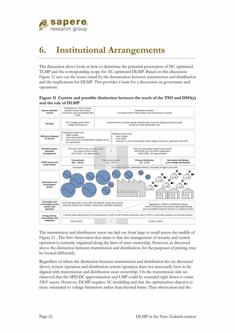
Page 32 DLMP in the New Zealand context
6. Institutional Arrangements
The discussion above looks at how to determine the potential penetration of DC optimised
TLMP and the corresponding scope for AC optimised DLMP. Based on this discussion
Figure 11 sets out the issues raised by the demarcation between transmission and distribution
and the implications for DLMP. This provides a basis for a discussion on governance and
operations.
Figure 11 Current and possible distinction between the reach of the TSO and DSO(s)
and the role of DLMP
The transmission and distribution assets are laid out from large to small across the middle of
Figure 11 . The first observation that arises is that the management of security and system
operation is currently organised along the lines of asset ownership. However, as discussed
above the distinction between transmission and distribution, for the purposes of pricing, may
be located differently.
Regardless of where the distinction between transmission and distribution lies (as discussed
above) system operation and distribution system operation does not necessarily have to be
aligned with transmission and distribution asset ownership. On the transmission side we
observed that the SPD DC approximation and LMP could be extended right down to some
33kV assets. However, DLMP requires AC modelling and that the optimisation objective is
more orientated to voltage limitations rather than thermal limits. That observation and the
Transmission
220 – 110 kV
Sub transmission
110 – 33 kV
Primary distribution
22 – 11 kV
Secondary distribution
(Low voltage distribution)
Transmission tends to be:
· higher voltage
· more interconnected
· have more active and distributed voltage sources
(i.e. generation)
Distribution tends to be:
· lower voltage
· more radial
· have less, or more concentrated, active voltage sources (i.e. generation and GXP)
TX/DX assets and
asset owners
Generation and
consumption asset
owners and
operators
System operator
current
Transpower Distribution networks, embedded networks, microgrids through to the meter
Transpower as TSO on service
provider contract with market.
Solution for least cost dispatch with
TLMP
Distribution networks.
(Concept of DSO in New Zealand only just starting to emerge)
TSO with TLMP across a broader reach
(e.g. down to 33 kV mesh)
Note TLMP = DC approximation
DSO (not necessarily network asset owner)
with DLMP (e.g. from 33 kV radial down)
Note DLMP = AC approximation
Possible system
operation
arrangements
SecurityTSO manages power flows,
voltage and frequency
Network owners currently operate networks with a focus on voltage and power quality
(Could be a DSO optimisation role)
Energy pricing,
reconciliation and
settlement
Difference between
TX and DX
Generation and
consumption
assets
?
Currently sales and purchase of all energy based on LMP at GXPs whether exposed to spot or FPVV or some other variations of financial contracts
TLMP at GXP DLMP in future?
Grid scale generation owners offer and dispatch energy and reserves
based on market rules. Ancillary services are contracted separatelyAggregators, retailers or distributors acquire
control of consumers discretionary generation/storage
and consumption assets for reserves or ancillary services.
?

DLMP in the New Zealand context Page 33
changes beginning to emerge at the low voltage level suggest that the case may emerge for a
distribution system operator (DSO) that is not necessarily the network asset owner.
The changes referred to here are well understood at a technology level. Consumers now have
access to EVs, battery storage and small-scale generation. It is also now possible for load
control to be accessed electronically by whoever consumers wish to provide access to and
load control will cover more than the traditional hot water heaters. The flexibility afforded by
discretionary generation, storage and consumption will be increasingly acquired by
aggregators, retailers or distributors who offer the most compelling arrangement. These
services may be deployed for the energy market, the national reserves market or ancillary
services at transmission or distribution level. Optimisation and coordination of these
activities at distribution level will not necessarily fall to the distribution network asset owner
in the future.
In this context, we need to be careful that the definition of DLMP is sufficiently broad to
ensure we consider a wide range of options for this economic optimisation. We are cognisant
that the objectives of smart grid infrastructure are the same objectives of DLMP. In fact, in a
modelling and economic sense, they are identical. Both seek to optimise (i.e. minimise cost
or maximise net societal benefit) the dispatch of assets and devices within the distribution
network. Both then seek to respond to changing conditions on the network based on the
marginal change in cost or net benefit at different locations.
We suspect that most people would envisage that DLMP means that the marginal value of
generation (or marginal cost of consumption) at different locations is published as a price;
and consumers, suppliers and the network operators respond to them. However, we contend
that smart grid optimisation systems are commensurate with DLMP, even though they may
not publish marginal prices per se. Where the response to a locational change in marginal
cost or net benefit is by a device on the network that is responding automatically to control
signals (pseudo dispatch instructions) from a smart grid system, the same outcome is
achieved. Where it is expected that the response will be entirely automated then it is not
necessary to publish prices. However, a reasonable expectation is that the owners of DER
receive a price that reflects the value of their service.
In the broadest sense, then, we believe it is important to contemplate both eventualities –
i.e., (i) individuals responding to published prices and/or (ii) automation responding to
dispatch instructions from an economic optimisation. Hence the decision to enforce DLMP
prices for settlement is not a fait accompli, but a decision that may or may not be taken by the
market designer, cognisant of the degree of automation, and the extent to which behavioural
response is expected.
The benefit of adopting this broader approach is that it allows us to contemplate
implementation options which are disaggregated, and permit some flexibility within the
distribution system. As outlined later, this allows the development, computation, and
informational effort to be spread across multiple parties, rather than being integrated into a
single modelling approach. But we reinforce that any proper economic approach to
optimising the dispatch of resources at the distribution level, in a way which is coordinated
with the grid level, should allow the publication of prices.
Below we consider the possible governance and operation models for DLMP.
Page 34 DLMP in the New Zealand context
6.1 Implementing DLMP under a DSO At present the role of DSO (as envisaged under a DLMP model) does not exist. Under
current arrangements (Code, connection contracts, Use of System Agreements, legislation
such as the Electricity Act 1992) TSO and limited versions of the private operator model are
practicable. Otherwise networks are currently operated by the owner (or an owner of a
separate network under an operating agreement). Network operation is not dynamic in the
way a DSO is expected to operate.
The need for a DSO reflects the shift from the traditional (security-driven) role of network
operators that network owners have carried out to a new (economically-driven, but security
constrained) role managing multiple sources of offtake and injection driven by consumer
preferences and arrangements with a variety of vendors. Consumer preferences may reflect
price, or more accurately the impact on cost of those decisions, but will also be a response to
a number of other influences. In many cases the prices consumers see would continue to be
fixed price variable volume prices bundled with distribution and transmission costs.
The need to account for network common quality and security, with multiple providers of
services, and in the context of maximising net societal benefit, will require a DSO role of
some form to be actively pursued. At the very least, even if the chosen philosophical
approach was to purely rely on consumers (or their service providers) responding to DLMP
price signals (rather than the formal establishment of platforms) it begs the questions of who
is going to calculate these prices (and how).
The more active the DSO management the more critical it will be for the dispatch activity of
the DSO to be coordinated with the national network. An active DSO could be given
responsibility for balancing the local system and coordinating that activity with national
balancing.
There are several possible ways local distribution networks could be more actively managed. For example, this could be through an increased role for the transmission system operator, network owners evolving into local system operators or the creation of new organisations to manage local networks independently. 35
Further, we have established that the DSO and the current network owner do not have to be one and the same organisation. We have also established that the boundary between the TSO’s jurisdiction and the DSO jurisdiction need not necessarily be the geographical distinction between the physical grid and the network areas. The question for this paper relates to practical considerations for implementing DLMP but we have also considered the wider question of how to ensure optimised power flow modelling at distribution level with a proliferation of assets and competing control of those assets at distribution level. Whatever the answer is will beg the question of whether there is a positive benefit to doing so. The UK National Infrastructure Commission suggests an active distribution system operator could be given responsibility for balancing the system at a local level in real time in the new distribution world we are entering into. There are three key benefits which could stem from this arrangement:
First, a DSO with a clear idea of what the local network needs at each moment in time will be able to purchase or procure these services to manage its system, creating revenue streams and market
35 UK National Infrastructure Commission Smart Power 2016
DLMP in the New Zealand context Page 35
signals to suppliers. It is currently difficult to put together a commercial business case for local level storage and demand flexibility measures, as their benefits are diffused across different parts of the system. This change will also incentivise the development of new and innovative business models, and save money for consumers by reducing or deferring the need for costly physical enhancements to the grid.
Second, better visibility of the network, combined with more monitoring, control and smart technologies means that network operators will be able to adapt to more complex and unpredictable electricity flows. This means that more distributed and intermittent generation will be able to connect to the networks at a lower overall cost to the system.
Third, it will enable better coordination between the transmission and distribution networks. A set of DSOs could have a role in ensuring the effective management of the interface with the transmission network and a coordinated system-wide approach. They could work with the transmission system operator to ensure that the benefits of new technologies such as storage and demand flexibility are maximised across the system as a whole, helping to coordinate what deploys when to ensure no detriment to local services. DSOs could operate local balancing markets, linked to the national balancing markets run by the SO. 36
Our definition of DLMP acknowledges the importance of locational marginal price signals as
incentives for welfare-maximising decisions. But we remain open-minded about the form in
which these prices are published and how they are used – this may be done through
automation or relying on behavioural response to price by consumers or their agents.
6.1.1 Establishing a DSO If DLMP was to be introduced across all distribution networks with a single model deployed
by all DSOs then a single rule book might be established along the same lines as the current
code for the wholesale market. In practical terms these provisions may be dealt with through
the current Code or a separate DSO code developed. If the latter approach was adopted
some of these provisions would be removed from the current Code. Matters to be
accounted for include:
Distribution Optimised Power Flow (DOPF)
• System for balancing energy and voltage
• Procurement of reserves
• Other ancillary services
• Publication of LMPs and treatment of LCE (if applicable)
Financial flows
• Clearing and settlements for energy, and ancillary services
Reconciliation
• Metering
• Volume reconciliation process
Operators
36 ibid
Page 36 DLMP in the New Zealand context
• Service provider arrangements
• Force majeure provisions
• Accountability requirements.
• Principal performance obligations
• Security of supply and emergency management
Asset owners
• Performance obligations of asset owners, arrangements concerning ancillary services
• Conditions of connection to network
• Use of System Agreements
6.2 Model 1 - TSO and Distribution System Operator(s) only
Many of the models proposed in the literature anticipate a DSO. Our definition of DSO is a
role that does not necessarily mean nor align with existing network ownership boundaries,
although it could. There could be many DSOs or there could only be one. The TSO and
DSO could be the same party, but taking clearly different roles.
We have established that the DLMP model is likely to be an AC model. Under a regime
with multiple DSOs it doesn’t automatically follow that each DSO uses the same
optimisation model although that might be a desirable approach.
We envisage that instructions and obligations would cascade downwards while information
disclosure obligations operate both ways. It doesn’t follow that the TSO and DSO models
are formally co-optimised but it is critical that they are coordinated in the sense that
protocols determine which party has first priority on security and ancillary service assets, as
well as that the price signal from the grid is appropriately incorporated into the economic
valuation of resources in the distribution network. There are requirements in place for the
provision of information between the current transmission and distribution operators but
will become more complex and more important as the load profile changes.
Under this model we envisage that the clearing and settlement arrangements for energy
would be an extension of current arrangements for reconciliation. With the increase in the
number of nodes at which settlement will occur, there may be impacts on the infrastructure
currently used for reconciliation and settlement; we have not estimated these.
6.3 Model 2 - TSO/DSO and ‘franchised’ aggregators using an approved model
This approach disaggregates one step further than the TSO/DSO model but still has high
levels of central coordination. Under this approach aggregators operate with DLMP models
but these models are tightly coupled with the DSO model. The obligations, protocols and
DLMP in the New Zealand context Page 37
prices between the TSO and DSO would cascade downwards to ensure the convergence of
optimal solutions37.
The aggregators may be required to use the DSO model and only provide appropriate input
data or the aggregators may be permitted to have their own model that meets a prescriptive
specification (relating to an objective of maximising economic welfare). The DSO may then
interact with the TSO wholesale model as per the TSO/DSO model.
As we move through these models we note that reconciliation and clearing and settlements
may become more complex. If DLMPs are published at lower voltage levels with franchised
aggregators using an approved model it starts to become more possible that the aggregator
reconciles and settles on a net position with the wholesale market. This becomes more likely
if the aggregator has a single point of connection such as a microgrid.
6.4 Model 3 - Private operators using proprietary locational models but meeting set standards
Under this approach there is no attempt to get the disaggregated models to “co-optimise”
with each other, other than through the DLMP price provided by the DSO to each operator.
Instead a standard for their individual optimisations is set, which the private operators
(individuals or aggregators of Distributed Energy Resources) need to meet. This standard
may be quite specific in setting the objective function of any model and the nature of the
model to be implemented, or the standard could be much less specific. However, it would
need to require that the model be optimised on a locational basis for it to meet the
requirement of achieving the same economic outcomes as DLMP.
Under this approach there would still be a DSO coordinating function but the DLMP
approach from the DSO could be very simple.
As above there may be a case for some sort of net reconciliation with private operators using
proprietary locational models for Model 3 and Model 4.
6.5 Model 4 - Private operators using proprietary locational models with communication protocols
This approach is similar to the private operator with set standards above but there is no
specificity about what the private operators are optimising nor any coordinated dispatch.
There is simply a requirement that the DSO has sufficient knowledge about what the private
operator is doing (through defined communications) in order to develop a forecast of net
demand or supply, and that the private operator is facing (and optimising on the basis of) a
37 We acknowledge that such an approach may not result in a globally optimal solution, but rather a locally
optimal solution.

Page 38 DLMP in the New Zealand context
distribution marginal loss-adjusted purchase or selling price, even if it is a simple approach
(e.g., marginal loss factor).
DLMP in the New Zealand context Page 39
7. Options assessed in terms of tasks and complexity
We have outlined above the many considerations that would need to be investigated before
determining an appropriate governance and operating model for the expansion of locational
marginal pricing beyond the current GXP boundary.
A key consideration we have reinforced is discovering where the “true” boundary between transmission and distribution lies, as this goes to whether LMP prices can be reliably produced from DC approximations to the optimal power flow model, or whether different modelling approaches are required. This is a primary task.
Beyond this, there are a range of potential implementation options. There is inevitably a
preliminary investigation phase where many of the key questions raised above would be
more rigorously assessed. At a high level, we now ask practically what would have to be
achieved under each of the options in order to obtain a full implementation. This will
inform what the “next steps” might be before determining the appropriate implementation
path.
Tasks common to all paths below include:
• Obtaining sufficient two-way flows of information between system operators and asset
owners about the new assets being modelled
• Ensuring appropriate telemetry and metering for new nodes.
• Changes to wholesale market participants’ processes so that settlement can take place at
the new pricing nodes
• Any Code changes required
• Insofar as the DLMP approach does not extend to the level where current average loss
factors are estimated, network companies would have to update their loss factors.
• Where prices are to be published, a process for pushing them to WITS or some
equivalent interface for participants.
• Determination of how the settlement surplus is dealt with
Beyond this, the tasks vary by option:
(i) Extend SPD into the sub-transmission network and retain as a DCOPF. Implementation time and complexity likely to be the lowest of the options (although not inconsiderable) as Transpower will have a process for incorporating new nodes into SPD. a. Obtain required asset owner information about network to be added to
SPD b. Model the new network in SPD, develop any required security constraints
etc c. Significant testing,
Page 40 DLMP in the New Zealand context
(ii) Extend SPD further into the distribution network and convert to ACOPF. We do not think this is currently practical and would need a watching brief on international developments around ACOPF models
(iii) Retain SPD as is, and allow other parties (EDBs, or new DSOs), to construct their own DCOPF for shallow parts of the sub-transmission networks. Aside from the design of an appropriate governance structure, this option would be more complex and time consuming than (i) above, since there are potentially multiple models being developed, although the information aggregation task would be more distributed and hence potentially simpler: a. The new “system operators” would need to construct new DCOPF models
and test them, as above b. How the multiple models interface with SPD would need to be determined
(iv) Retain SPD as is, or pursue option (i), and allow other parties (EDBs, or new DSOs), to pursue their own AC OPF models. As for (ii), we do not think this is currently practical and would need a watching brief on international developments around ACOPF models
(v) Retain SPD as is, and allow other parties (EDBs, or new DSOs), to pursue their own (improved) LMP approximations such as marginal loss factors (on some granularity) applied to the GXP price (as a replacement for average loss factors) and/or administered congestion pricing based on smart metering data. The complexity of this task depends on the depth of the prices (and, presumably, the remainder of the “gap” between the DLMP assessment and the ICP), which in turn depends on the accuracy of the metering at different locations. However, presumably EDBs have sufficient metered information to develop average loss factors, and that metering information is available on a higher time resolution, which should allow decent estimates of marginal loss factors.
7.1 Investigations required for each broad option
If the Authority wished to extend TLMP into the sub-transmission network, it would need to:
• Determine an appetite for error, in the New Zealand network context, inherent in DC
approximations
• Carry out an empirical study of sub-transmission (to delineate the grey area) starting
with >66kV, remaining sub-transmission mesh, remaining sub-transmission radial, and
(if results are favourable) maybe 11kV mesh to determine the suitability for DC
approximations
• If the Authority wanted to implement LMP in those parts of the network that satisfy
the criteria for DC approximation via an expansion of SPD, it would need to carry out
an empirical study of SPD to:
Test whether SPD has the capability to incorporate new nodes and remain within
the appetite for error
Based on the allowable error, define the X/R and flat voltage criteria for inclusion
to SPD.
DLMP in the New Zealand context Page 41
• If SPD cannot be acceptably expanded, and/or the Authority wishes to pursue a
different governance model, that model would need to be designed with a separate
DCOPF(s).
• Determine how required network information will flow between asset owners and the
TSOs
If the Authority wanted to pursue DLMP in the “true” distribution network, it would need
to:
• Assess the full governance and operating implications of DLMP down to low voltage
distribution. This includes the potential for the establishment of distribution system
operator(s), and the various models for how they may interface with private aggregators
and smart grid optimisation schemes, such as peer-to-peer distribution services and
virtual power plants
• Keep a watching brief on global developments in smart grids and the use of ACOPF
for DLMP.
• Investigate the practicality, and potentially modelling, of average marginal loss
approximations between the defined TLMP boundary and the pricing zone.
• Investigate the practicality, and potentially modelling, of administered congestion
pricing using smart meter information to reflect congestion – whether as a result of
thermal, power quality or voltage limitations, between the defined TLMP boundary and
the pricing zone.
For either of the above implementation paths, the Authority would also need to investigate:
• The available information on network assets required for construction of either a
DCOPF, ACOPF or any other approximation used. This would inform an assessment
of the practicality for our two options, i.e., whether any of the following would be
required:
(a) A survey any lines and substations for which there is insufficient information
(b) Installations of all required telemetry where it doesn’t currently exist
(c) Installation code compliant metering to every zone substation, and possibly on to
every 11kV feeder circuit
• Investigate required Code changes, especially around clearing, settlement and
reconciliation, as well as grid definition and requirements for SPD
• Determine how any settlement surpluses arising from the new nodes for settlement is
dealt with