1

An Imperfect Multi-Item Single Machine production system with Shortage, Rework,

and Scrapped Considering Inspection, Dissimilar Deficiency Levels, and Non-Zero

Setup Times

Amir Hossein Nobil1, Amir Hosein Afshar Sedigh

2, Sunil Tiwari

3, H.M. Wee

4*

1Faculty of Industrial and Mechanical Engineering, Qazvin Branch, Islamic Azad University,

Qazvin, Iran 2Information Science, University of Otago, Dunedin, New Zealand

3The Logistics Institute-Asia Pacific, National University of Singapore, 21 Heng Mui Keng Terrace,

#04-01, Singapore 119613 4Department of Industrial and Systems Engineering, Chung Yuan Christian University, No. 200,

Chung Pei Road, Chung Li District, Taoyuan City, 32023, Taiwan

Abstract

In this paper, we consider a deficient production system with permissible shortages. The

production system consists of a unique machine that manufactures a number of products that

a part of them are imperfect in form of rework or scrap. These defective products are

identified by 100% inspection during production, then, they are whether reworked or

disposed of after normal production process. Like real-world production systems, there are

diverse kinds of errors creating dissimilar breakdown severity and rework. Moreover,

reworks have non-zero setup times that makes the problem closer to real-world instances

where machines require some preparations before starting a new production cycle. Thus, we

introduce an economic production quantity (EPQ) problem for an imperfect manufacturing

system with non-zero setup times for rework items. The rework items are classified into

several categories based on their type of failure and rework rate. The aim of this study is to

obtain optimum production time and shortage in each period that minimizes total inventory

system costs. Convexity of the objective function and exact solution procedure for the current

nonlinear optimization problem are also proposed. Finally, a numerical example is proposed

to assess efficiency and validation of proposed algorithm.

Keywords: Lot sizing; imperfect manufacturing; multiple rework; single machine; exact

algorithm

* Corresponding author

E-mail: weehm@cycu.edu.tw (H.M. Wee*) other authors emails: amirhossein.nobil@yahoo.com (A.H. Nobil), amir.afshar

@postgrad.otago.ac.nz (A.H.A. Sedigh), sunil.tiwari047@gmail.com (S. Tiwari)

2

1. Introduction

For any manufacturing organization the supply chain, Inventory and production management

are more vital to achieve success. To achieve the goals of operation management, each

company should effectively utilize resources and try to minimize costs as well as possible. In

today’s competitive environment every organization wants to make sure that their customers

are satisfied with the quality of their products. As today nobody (customers) wants to

compromise with the quality of the product. In the classic EPQ model assumes that during a

production run a 100% perfectly products are manufacture, which is far from the reality.

There are so many reasons due to which at few percent of imperfect items are produces.

These situations are like the breakdown of machine, interruption in manufacturing process

etc. So one can’t ignore this situation (imperfect production), as it has direct side effect on

organization’s reputation and good-will. Employing mathematical optimizations for

inventory management dates back to more than a century ago when Ford Whitman Harris [1]

introduced classical economic order quantity (EOQ) inventory model in 1913. This model is

the foundations of lot-sizing models; and one can consider Harris as the founder of modern

inventory studies [2].

In 1918, Taft [3] proposed economic production quantity (EPQ) by extending

aforementioned inventory model for a manufacturer that produces an item at a constant rate.

The main drawback of these inventory models is their impractical assumptions as a result;

several studies relaxed these assumptions to make these models more applicable in real-world

instances. For example, Hadley and Whitin [4] proposed a summary of the EOQ inventory

model and extended this model by taking account of shortage. Moreover, Parker [5]

investigated reorder point and reorder quantities for an inventory system with stochastic

demand and permissible backorder. On the other hand, Yao and Lee [6], Lee and Yao [7],

and Björk [8] are examples of developing the EOQ model for instances that fuzzy numbers

are employed to approximate model parameters. Moreover, Silver [9], Maddah and Jaber

[10], and Khan et al. [11] considered stochastic uncertainties in parameters under several

assumptions.

Flawless products and perfect quality is another impractical assumption in basic

EOQ/EPQ inventory models. In modern-day organizations deteriorating items has drawn

attentions to them in different forms, i.e. scrapped, defective, rework, obsolescence and so

forth. One of the first instances of inventory models with deteriorating items was proposed in

Whitin [12] where items became obsolete during time. Aggarwal and Jaggi [13] studied

permissible delay in payments with deteriorating products. Wu et al. [14] studied an

3

inventory system consists of non-instantaneous deteriorating items with partial backordering.

Chang et al. [15] developed the aforementioned model by maximizing total profit, instead of

minimizing cost per time unit, considering maximum inventory level constraint. Wu et al.

[16] addressed deteriorating items with expiration dates and trade credit when trade credit

increased revenue as well as opportunity cost and default risk. Some recent studies that

investigated inventory management with deteriorating items under different policies are Sett

et al. [17], Wu and Zhao [18], Mokhtari et al. [19], Wu et al. [20], Shah and Cárdenas-Barrón

[21], and Teng et al. [22]. Recently, Dobson et al. [23] proposed an EOQ inventory model for

deteriorating items with a single product where consumers’ demand rate linearly decreased as

a function of product’s age.

Furthermore, EPQ inventory model is extended by relaxing perfect production systems

in different studies. Salameh and Jaber [24] considered an imperfect production system that

poor-quality products could be sold at a lower price after 100 percent inspection. Afterwards,

Goyal and Cárdenas-Barrón [25] proposed a simpler approach to solve aforementioned

problem with near optimal solutions. Wee et al. [26] generalized Salameh and Jaber [24] by

modelling an imperfect production system in an uncompetitive market where shortage was

permitted and fully backordered. Haji et al. [27] developed a model and its optimization for

an imperfect production system with reworks, where machine required a setup before starting

rework procedure. Recently, Nobil et al. [28] indicated the possibility of shortage occurrence

during setup time in former model and proposed a modified algorithm to overcome this

deficiency. Cárdenas-Barrón [29] studied an imperfect production system with rework and

planned backorders. Hsu and Hsu [30], Farhangi et al. [31], Cárdenas-Barrón et al. [32], Shah

et al. [33], Jaggi et al. [34] and Jaggi et al. [35] are some recent inventory management

instances with imperfect products.

Moreover, producing several items on a machine is another realistic extension of EPQ

inventory model. Rogers [36] proposed the first instance of this kind of inventory model.

Taleizadeh et al. [37] developed the aforementioned model with respect to shortage and

imperfect production system with interruptions, scrapped items, and rework. Pasandideh et al.

[38] proposed an EPQ inventory model for an imperfect production system with permissible

shortage. In their study, they considered a machine produced various quality items, i.e.

perfect, scrapped, and rework. They considered diverse failure levels with their own rework

procedures. This classification of reworks made the inventory model more realistic by

considering various kinds of production errors. Nobil et al. [39], considered utilization-

allocation policy in an imperfect manufacturing system producing multiple products on

4

several machines using single-machine properties and common cycle length to reduce

calculation efforts in a hybrid genetic algorithm. Nobil and Taleizadeh [40], Nobil et al. [41],

and Nobil et al. [42] are some recent inventory management studies with single machine

production system.

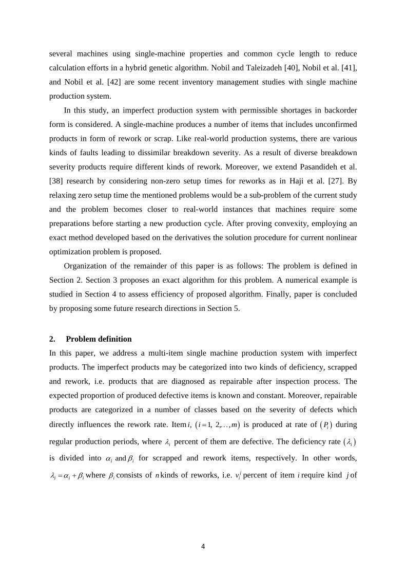
In this study, an imperfect production system with permissible shortages in backorder

form is considered. A single-machine produces a number of items that includes unconfirmed

products in form of rework or scrap. Like real-world production systems, there are various

kinds of faults leading to dissimilar breakdown severity. As a result of diverse breakdown

severity products require different kinds of rework. Moreover, we extend Pasandideh et al.

[38] research by considering non-zero setup times for reworks as in Haji et al. [27]. By

relaxing zero setup time the mentioned problems would be a sub-problem of the current study

and the problem becomes closer to real-world instances that machines require some

preparations before starting a new production cycle. After proving convexity, employing an

exact method developed based on the derivatives the solution procedure for current nonlinear

optimization problem is proposed.

Organization of the remainder of this paper is as follows: The problem is defined in

Section 2. Section 3 proposes an exact algorithm for this problem. A numerical example is

studied in Section 4 to assess efficiency of proposed algorithm. Finally, paper is concluded

by proposing some future research directions in Section 5.

2. Problem definition

In this paper, we address a multi-item single machine production system with imperfect

products. The imperfect products may be categorized into two kinds of deficiency, scrapped

and rework, i.e. products that are diagnosed as repairable after inspection process. The

expected proportion of produced defective items is known and constant. Moreover, repairable

products are categorized in a number of classes based on the severity of defects which

directly influences the rework rate. Item 1, 2,, , ii m is produced at rate of iP during

regular production periods, where i percent of them are defective. The deficiency rate i

is divided into and i i for scrapped and rework items, respectively. In other words,

ii i where i consists of n kinds of reworks, i.e. jiv percent of item i require kind j of

5

rework and 1,2, ,j n . So, total proportion of product i that requires rework i can be

stated as sum of jiv , i.e.

1 2

1

. . ..n

ni i

ji ii

j

iv orv v v

So we have:

1 2 ni i i i i i iv v v (1)

Furthermore, in the proposed inventory system all items are produced by one

machine, this property causes the following equation to be held:

1 2 3 mT T T T T (2)

The following notations are employed to model the proposed non-linear single-machine

inventory control problem with 𝑚 kinds of items and 𝑛 types of rework.

ic Production cost to manufacture each item kind 1,2, ,, . ii m

io Inspection costs per item kind 1,2, ,, . ii m

id Disposal costs per item kind 1,2, ,, . ii m

jir Rework costs for item kind i with fault type j , 1,2, , & 1,2, , .i m j n

ih Holding costs per year per item kind 1,2, ,, . ii m

iL Shortage costs per year per item kind 1,2, ,, . ii m

iA Set-up costs per regular production cycle to produce item kind 1,2, ,, . ii m

iB Set-up costs per rework cycle for all rework types associated with item kind

1,2, ,, . ii m

its Set-up time per regular production cycle to produce item kind 1,2, ,, . ii m

iG Set-up time per rework cycle for all rework types associated with item kind

1,2, ,, . ii m

6

iP Production rate for item kind 1,2, ,, . ii m

iD Demand rate for item kind 1,2, ,, . ii m

i Disposal rate of produced item kind 1,2, ,, . ii m

jiv Percentage of produced item kind i that requires rework type ,j

1,2, , & 1,2, , .i m j n

i Percentage of produced imperfect product kind 1,2, ,, . ii m

ji Rework rate for rework type j associated with item kind ,i

1,2, , & 1,2, , .i m j n

T Cycle-length.

N Number of cycles in a year.

iQ Quantity of produced item kind i per cycle, 1,2, , .i m

iS Quantity of shortage for item kind i per cycle, 1,2, , .i m

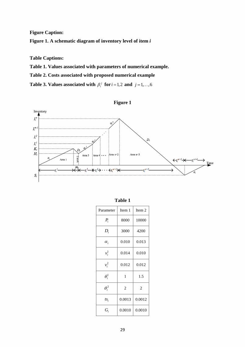
<Insert figure 1 here>

A schematic diagram of inventory position for this model is represented in Figure 1. As it is

demonstrated by Figure 1, production rate of item 𝑖 during regular cycle is iP where i

percent of them are defective, consequently, production rate on non-defective items kind i per

cycle equals to 1 i iP . On the other hand, production rate of non-defective items should be

more than or equal to its demand rate iD , in other words we have:

1       1 0i i i i i i iP D or e P D (3)

After accomplishment of regular production cycle and inspection, scrapped items are

disposed and rework process should be initiated. In this study, we assume that rework process

has a non-zero setup time equal to regular production setup time. Moreover, for sake of

simplicity and as a consequence of independency of setup times we consider one setup time,

i.e. iG , before starting all types of rework for item kind i . During setup time, no item is

7

produced and item i consumed with rate of iD . Then, the rework processes initiate with rates

of 1 2, ,..., ni i iand during 2 3 1, ,.... n

i i iandt t t periods, respectively where during these periods

no scrapped item is manufactured. Moreover, it is logical to assume that the rework process

of products does not require more times than their corresponding regular production times. In

other words, the rework rate for a product is greater than or equal to its regular production

rate, i.e. 1ji . Consequently, the demand rate iD for product i is less than or equal to its

rework production rate .ji iP In other words,

      0i

j j ji i i i i i iP D or a P D (4)

Based on Figure 1 and aforementioned conditions, inventory level at the end of each rework

process can be stated as:

i ii i

i

e QK S

P (5)

i ii i i i i i i

i

e QH K G D S G D

P (6)

1 1 1 11

1 1

i i i i i i i ii i i i i

ii i i i

a v Q e Q a v QI H S G D

PP P

(7)

2 2 1 1 2 22 1

2 1 2

i i i i i i i i i i ii i i i i

ii i i i i i

a v Q e Q a v Q a v QI I S G D

PP P P

(8)

So the following is obtained:

1

; 1, 2, ,

j j jj i i i i i

i i i i ji i ir

e Q a v QI S G D j n

P P

(9)

Moreover, based on the inventory level and Figure 1 each period length can be stated as:

1 i i ii

i i i

K Q St

e P e (10)

1 12

1 1

i i i ii

i i i

I H v Qt

a P

(11)

8

2 1 23

2 2

i i i ii

i i i

I I v Qt

a P

(12)

Consequently, we have:

11 ; 1,2, ,

j j jj i i i i

i j ji i i

I I v Qt j n

a P

(13)

Thus:

1n

n i ii n

i i

v Qt

P

(14)

On the other hand, we know that:

2

1

jn j jn i i i i i i ii i j

i i i i i i ir

I e Q S a v Qt m

D D P D D P

(15)

3n ii

i

St

D

(16)

4n ii

i

St

e

(17)

Based on the above-mentioned conditions, a period length can be obtained as:

1 2 3 1 2 3 4n n n ni i i i i i i i iT T t m t t t t t t (18)

Moreover, based on the (A.4) stated in Appendix A, a cycle length can be calculated as:

1 i i

i

QT

D

(19)

And:

1

ii

i

D TQ

(20)

9

2.1. Objective function

The objective function of proposed problem is to optimize total inventory costs including

annual setup costs for regular production cycles, annual setup costs for reworks, annual

production costs, annual inspection costs, annual disposal costs, annual rework costs, annual

shortage costs, and annual holding costs. As it is mentioned before, setup cost for regular

production cycle for item kind i is iA . Moreover, each year consists of N cycles and annual

setup costs SC for regular production of all items is stated as:

1 1

m mi

i

i i

ASC NA

T

(21)

On the other hand, setup cost for rework associated with item kind i per cycle is iB

and a year consists of N cycles. So, annual setup costs UC for reworks of all items is as

follows:

1 1

m mi

i

i i

BUC NB

T

(22)

Production costs per item kind i equals to iQ . As a result, production costs per cycle

can be stated as i ic Q and total production costs per year PC is:

1 1

m mi i

i i

i i

c QPC Nc Q

T

(23)

Substituting iQ from Eq. (20) in Eq. (23) we have:

1 11

m mi i

i i

ii i

D cPC Nc Q

(24)

Inspection costs per item kind i is io and production quantity of this kind of item per

cycle is iQ . So, inspection costs per cycle is i io Q and annual inspection costs IC equals to:

10

1 11

m mi i

i i

ii i

D oIC No Q

(25)

Disposal costs per item kind i is id and quantity of produced items require disposal

per cycle is i iQ . So disposal costs per cycle is i i id Q and annual disposal costs DC can be

stated as:

1 11

m mi i i

i i i

ii i

D dDC Nd Q

(26)

Rework costs of type j per item kind i is jir and quantity of produced items require

this type of rework per cycle is ji iv Q . So rework costs type j per cycle is j j

i i ir v Q and annual

rework costs RC can be stated as:

1 1 1 11

m n m n j jj j i i i

i i i

ii j i j

D r vRC Nr v Q

(27)

As it can be seen in figure 1, the backordered demands for item kind i can be stated as

3 4 / 2n ni i iS t t . Knowing that annual shortage costs for product kind i is iL , annual shortage

costs BC is:

3 4

12

n nmi i i i

i

NL S t tBC

(28)

Substituting 3nit and 4n

it by Eq. (16) and Eq. (17) respectively, we have:

2

12

mi i i i

i ii

L e D SBC

D e T

(29)

Annual holding costs for item kind i is ih , and with respect to the area under the curve

in figure 1, annual holding costs (𝐻𝐶) can be stated as:

11

1 2 1 2 31

1 1 21

2 2 2 2

...2 2

i i i i i ii i ii im

in n n n ni i i i i i

H I t I I tK H GK t

HC NhI I t I t

(30)

This equation can be stated as follows, for calculations see Eq. (B.10) of Appendix B:

2

2

2 1

2 21 0

1 1

1 1

1 2 22 1

2 1 1

1 2

i i i i i i ii i i i i i i

i i i ii i

jn j y yi ii i i i i

i j yi i i ij yi i

n nj j ji i i i i i

i j ji i i ij j

h e h P Sh e G D h G SHC T

P e D T TP

h Dh e v a vS T

P P

h G D v a vD

P

1 1

2

2 21 1

2 22

2 2 21 1

1

1 2

1

21

1

2 1

n nj j ji i i i i

ij ji i ii ij j

n nj j ji i i i i i

j jii ij ji i

j jn n j ji ii i i i

jj

i ij ji i i

h D v a vS

P D

h e D v a vT

DP

a vh D a vT

DP

(31)

Finally, based on Eqs. (21), (22), (24), (25), (26), (27), (29), and (31) annual total cost

can be calculated as follows:

231 2 4 5 6

1 1 1 1 1 1

m m m m m mii i

i i i i i i

i i i i i i

SSTC T S

T T T

(32)

where,

11

1 11 12

n j jn nj j j i i i i i i iji i i i i i

i i i j ji i ii ij j

D c o d r vh G D v a v

e DP

(33)

12

2

2

2 21 1

2 22

2 2 21 1

2 1

2 2 21 0

1

21

1

2 1

1 0

1 2 1

n nj j ji i i i i i

i j jii ij ji i

j jn n j ji ii i i i

jj

i ij ji i i

jn j y yi i i i ii i i

j yi ij yi i i i

h e D v a v

DP

a vh D a v

DP

h D h ev a v

P P

; 1,2, ,i m

(34)

3 0; 1,2, ,i i iA B i m (35)

4 0; 1,2, ,2

i ii

h Gi m (36)

5

1 1

10; 1,2, ,

1 2 2 1

n nj j ji i i i i i i

i j ji i i i ii ij j

h D v a v h ei m

P D P

(37)

6 10; 1,2, ,

2 2

i i i i i i

i

i i i i

L e D h Pi m

D e e D

(38)

2.2. Constraints

In the proposed problem, the main constraint addresses the production capacity of machine.

This constraint expresses that summation of production time for all items and their setup time

should be less than or equal to permissible production time of machine. In other words, we

have:

14

1 1

m nj n

i i i i

i j

t t ts G T

(39)

This constraint can be stated as follows, for detailed calculations see inequality (C.4) of

Appendix C:

1

1 11 1

1

m

i ii

jm n

i i

ji ji i i

ts GT

D v

P

(40)

13

Other constraints restrict shortage at rework setup time. In other words, we have 𝑚

constraints to prepare machine for rework, i.e. equal to number of items. With respect to

Figure. 1 we have:

0; 1,2,..,iH i m (41)

By employing Eq. (6) the following should be held:

0; 1,2,..,i ii i i

i

e QS G D i m

P (42)

Substituting iQ by Eq. (20) we have:

0; 1,2,..,

1

i ii i i

i i

e DTS G D i m

P

(43)

Therefore,

10;   1,2,..,

i i i i i

i i

S G D PT i m

e D

(44)

2.3. Final model

Based on the objective function proposed in Eq. (32) and constraints proposed in inequalities

(40) and (44), final model of the proposed problem is as follows:

231 2 4 5 6

1 1 1 1 1 1

m m m m m mii i

i i i i i i

i i i i i i

SSMinTC T S

T T T

14

. :S t

1

1 11 1

1

m

i ii

jm n

i i

ji ji i i

ts GT

D v

P

10; 1,2,..,

i i i i i

i i

S G D PT i m

e D

0T

0; 1,2,..,iS i m

(45)

3. Solution method

In this section we propose a solution method to optimize proposed non-linear programming

model. To do so, first we prove the convexity of model (45) by investigating objective

function. It is worth mentioning that all decision variables are continuous and constraints are

in linear form. As it can be seen in Appendix D the quadratic form of objective function (45)

is semi-positive. So, model (45) is convex and using partial differentials we can obtain

optimum values for decision variables as follows:

4 65 2

0; 1,2,..,i i ii

i

STCi m

S T T

(46)

So,

5 4

6; 1,2,..,

2

i ii

i

TS i m

(47)

Moreover, by differentiating of objective function (45) according to T we have:

23

2 4 6

2 2 21 1 1 1

0m m m m

ii ii i i

i i i i

SSTC

T T T T

(48)

Then,

15

23 4 6

2 1 1 1

2

1

m m m

i i i i ii i i

m

ii

S ST

(49)

Substituting iS by Eq. (47) we have:

24

3

61 1

25

2

61 1

4

4

m m i

ii ii

m m i

ii ii

T

(50)

Based on the obtained solutions from Eqs. (47) and (50) optimum values associated with

model can be obtained using following algorithm:

Step 1- If 1 1

1 01

m n ji i

ji i ii j

D v

P

, go to Step 2. Otherwise, problem is infeasible and

go to Step 14.

Step 2- If

24

3

61 1 4

m mi

i

ii i

and

25

2

61 1 4

m mi

i

ii i

were simultaneously positive or

negative go to Step 3. Otherwise, problem is infeasible and go to step 14.

Step 3- Calculate T from (50) and go to Step 4.

Step 4- Based on the obtained values ofT , calculate shortage quantities associated with items

using (47) and go to Step 4.

Step 5- If 0iS for all 1,2, ,i m then go to Step 9, else go to Step 6.

Step 6- If 0iS ; 1,2, ,i m calculate4

5

ii

i

TL

, else for 0iS let 0iTL and go to Step 7.

Step 7- Calculate T using 1 2, , , mT Max TL TL TL then go to Step 8.

Step 8- Calculate iS for all 1,2, ,i m employing Eq. (47) with respect to T then go to step

9.

Step 9- Calculate values of GT and ; 1,2, ,XiT i m employing the following equations:

16

1

1 11 1

1

m

i iiG j

m ni i

ji ji i i

ts GT

D v

P

(51)

1; 1,2,..,

i i i i iXi

i i

S G D PT i m

e D

(52)

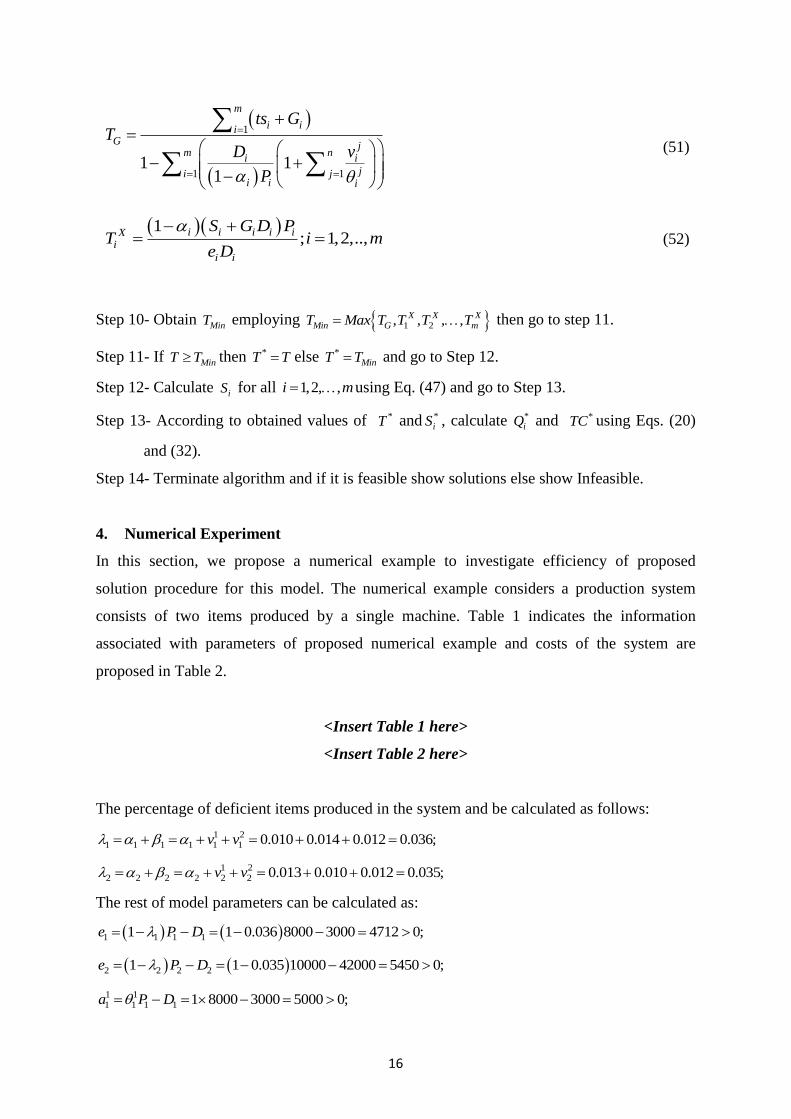
Step 10- Obtain MinT employing 1 2, , , ,X X XMin G mT Max T T T T then go to step 11.

Step 11- If MinT T then *T T else *MinT T and go to Step 12.

Step 12- Calculate iS for all 1,2, ,i m using Eq. (47) and go to Step 13.

Step 13- According to obtained values of *T and *iS , calculate *

iQ and *TC using Eqs. (20)

and (32).

Step 14- Terminate algorithm and if it is feasible show solutions else show Infeasible.

4. Numerical Experiment

In this section, we propose a numerical example to investigate efficiency of proposed

solution procedure for this model. The numerical example considers a production system

consists of two items produced by a single machine. Table 1 indicates the information

associated with parameters of proposed numerical example and costs of the system are

proposed in Table 2.

<Insert Table 1 here>

<Insert Table 2 here>

The percentage of deficient items produced in the system and be calculated as follows:

1 21 1 1 1 1 1 0.010 0.014 0.012 0.036;v v

1 22 2 2 2 2 2 0.013 0.010 0.012 0.035;v v

The rest of model parameters can be calculated as:

1 1 1 11 1 0.036 8000 3000 4712 0;e P D

2 2 2 21 1 0.035 10000 42000 5450 0;e P D

1 11 1 1 1 1 8000 3000 5000 0;a P D

17

2 21 1 1 1 2 8000 3000 13000 0;a P D

1 12 2 2 2 1.5 10000 4200 10800 0;a P D

2 22 2 2 2 2 10000 4200 15800 0;a P D

Moreover, ; 1, ,6ji j can be calculated employing Eqs. (33) - (38). The calculated values

for ji is proposed in Table 3.

<Insert Table 3 here>

Now, we calculate optimum solution for numerical example using proposed algorithm in

section 3 as follows:

Step 1- since

2 2

1 1

1 0.8173 11

ji i

ji i ii j

D v

P

go to Step 2.

Step 2- since both

24

3

61 1

5099.94

m mi

i

ii i

and

25

2

61 1

351.674

m mi

i

ii i

are

positive go to Step 3.

Step 3- T is calculated as follows:

24

3

61 1

25

2

61 1

4

3.80821661358787;

4

m m i

ii ii

m m i

ii ii

T

and go to Step 4.

Step 4- shortage values associated with each item are as follows:

5 4 5 41 1 2 2

1 26 61 2

0; 0;2 2

T TS S

go to step 5.

Step 5- since 1 2 0S S go to step 9.

Step 9- values of 1 2, , & X XGT T T are obtained as follows:

1

1 1

0.0246286036910265;

1 11

m

i iiG j

m ni i

ji ji i i

ts GT

D v

P

18

1 1 1 1 1

1

1 1

10.00168085688321865;X S G D P

Te D

2 2 2 2 2

2

2 2

10.00181103298935632;X S G D P

Te D

and go to Step 10.

Step 10- MinT is obtained as 1 2, , 0.0246286036910265X XMin GT Max T T T and go to Step 11.

Step 11- since MinT T we have * 3.80821661358787T T and go to Step 12.

Step 12- we obtain *iS with respect to calculated *T as follows:

5 * 4 5 * 4* *1 1 2 21 26 6

1 2

0; 0;2 2

T TS S

and go to Step 13.

Step 13- *iQ and *TC can be calculated based on the *T and *

iS obtained in former steps as

follows:

** 11

1

11540.0503442057;1

D TQ

** 22

2

16205.1770790973;1

D TQ

2*3 *

* 1 2 * 4 5 * 6

* * *1 1 1 1 1 1

$3094815.42042686m m m m m m

ii ii i i i i i

i i i i i i

SSTC T S

T T T

5. Conclusion and suggestions

In this study, we investigated a defective single-machine manufacturing system for several

commodities. The manufactured products may have problems with operator error, raw

materials quality and machine failure. Therefore, a percentage of the production may have a

percentage of unacceptable quality. These defective products are identified by 100 percent

inspection during production, and they are reworked or disposed of after normal production

process. Goods that require rework were classified into several categories based on their type

of failure, each with a different rework rate. In this system, there is a setup time to

manufacture each item on the machine in a normal cycle; in the rework cycle, a new setup

time is incurred. This study presents a single machine lot-sizing problem for an imperfect

manufacturing system with scrap and rework under non-zero setup times for rework items.

The reworks are classified into several categories based on the type of failure and rework

rate. Considering aforementioned conditions and permissible shortage backordered, the

19

proposed problem was modelled as a non-linear programming model. The convexity of this

model was proved and an exact algorithm was proposed. Finally, a numerical example was

given to assess the effectiveness of the proposed algorithm under different conditions.

5.1. Managerial insights

Taking into account the behavioral factors, this study investigates a fairly practical problem.

Therefore, the research of this study can provide insights for production managers and

planners in their decision-making. The nonlinear lot-sizing model of this research integrates

the production decisions, inventory and rework. Thus, the model provides a good framework

for the imperfect manufacturing system with scrap and rework

5.2. Limitations and future directions

This research only considers a deficient manufacturing system with permissible shortages.

The production system consists of a single machine that manufactures items with a certain

percentage of defective items that can be rework or throw away as scrap. For future work,

one can consider different marketing and pricing policies with budget and storage space

constraints. One can also consider the impact of information sharing between the

manufacturer and the end user.

Appendix A. Calculating cycle length

Based on Eq. (18) the production cycle length is:

1 2 3 1 2 3 4n n n ni i i i i i i i iT T t G t t t t t t (A.1)

Moreover, based on Eqs (10) to (17) we have:

1 2

1 21

1 1

1

jn j ji i i i i i i i i i i i i i i i

i in ji i i i i i ii i i i i i i i ir

j jj j ji i i i i i i i

j ji i i i i i i ir r

i i i

i i i

Q S v Q v Q v Q e Q S a v Q S ST G G

P e D P D D eP P P D P

Q e Q v Q a v Q

P D P P D P

Q e Q

P D P

1

j j j ji i i

j ji i ir

v a v

D

(A.2)

Employing Eqs. (3) and (4) the following is held:

20

1 1

1 1j jj ji i i ii i i i i i i

i i i i i i ir r

P PQ Q v P Q v PT

P D P D P D D

(A.3)

Substituting i from Eq. (1) in Eq. (A.3) we have:

1 1 1

1 1j j jj j ji i i ii i i i i i i i i i i

i i i i i i i i ir r r

P QQ v P Q P P v P v PT

P D D P D D D D D

(A.4)

Appendix B. Calculating the holding cost

Based on Eq. (30) the production cycle length is:

3 4 51 2

1 2 1 2 3 2 3 41

231

1 1 2

2 2 2 2 2

2 2

Area Area AreaArea Area

i i i i i i i i ii i ii im

i AreanAreani

n n n n ni i i i i

H I t I I t I I tK H GK t

HC Nh

I I t I t

(B.1)

Now, we calculate the specified areas in Eq. (B.1) to obtain a general relation for

holding costs as follows:

2 21

2

1 1

2 2 22

i i ii i i i i i i ii

i i i i ii

e Q SK t e Q Q S Q SArea S

P P e P eP

(B.2)

2

22 2

i i i i ii i ii i

i

K H G D Ge G QArea G S

P

(B.3)

21 2 1 12 21 1 1

2 1 1 1 2 21

32 2 2

i i i i ii i ii i i i i i i i

i ii i ii i i

H I t a ve Q Qv Q S v D G Q vArea

P PP P

(B.4)

1 2 3 2 2 2 2

2 2 2 2

22 22 2 1 1 2

2 2 2 1 22

42 2

2

i i i i i i i i i i i i i

i ii i ii

i ii i i i i

i ii ii

I I t e Q v Q S v D G Q vArea

P PP

a vQ Q a v v

P P

(B.5)

21

22 3 4 3 32 23 3 3

2 3 3 3 2 23

2 21 1 3 2 2 3

2 1 3 2 2 3

52 2 2

i i i i ii i ii i i i i i i i

i ii i ii i i

i ii i i i i i

i i i ii i

I I t a ve Q Qv Q S v D G Q vArea

P PP P

Q Qa v v a v v

P P

(B.6)

The areas (5) to (𝑛 + 2) can be stated as follows:

1 1 2

2

22 2 1

2 2 20

22 2

; 1,2, ,2

j j j j j ji i i i i i i i i i i i i

j j ji ii i ii

j j jj y yi ii i i i i

j yj

i iyi ii

I I t e Q v Q S v D G Q vArea j

P PP

a vQ Q v a vj n

P P

(B.7)

On the other hand, we have:

22

1

1 3

2 2 2

jn n n n j ji i i i i i i i i

i i i ji i i i ir

I t I I e Q a v QArea n S G D

D D P P

(B.8)

Finally, annual holding costs with respect to Eqs. (B.2) to (B.8) are as follows:

2 2

1

2 1

21 0 1 1

1 1

1 1

2 2 2 2

2

1

2

mi i i i i ii i i i i i i i i

i i i i i i ii

jn n nj y y j j ji i i i i i i i i

ij y j jii i i ij y j ji

n nj ji i i i

ji iij j

e Q P Sh e G Q G S e S QHC

T P PD e D PD

Q v a v G Q v a vD

PP

S Q v a v

P D

2

21 1

2 22

2 21 1

1

2

1

2

n nj j j ji ii i i i

j j jii i ij ji

j jn n j ji ii i i

jj

i ij ji i

e Q v a v

DP

a vQ a v

DP

(B.9)

Moreover, substituting iQ from Eq. (20) in Eq. (B.9) we have:

22

2

2

2 1

2 21 0

1 1

1 1

1 2 22 1

2 1 1

1 2

i i i i i i ii i i i i i i

i i i ii i

jn j y yi ii i i i i

i j yi i i ij yi i

n nj j ji i i i i i

i j ji i i ij j

h e h P Sh e G D h G SHC T

P e D T TP

h Dh e v a vS T

P P

h G D v a vD

P

1 1

2

2 21 1

2 22

2 2 21 1

1

1 2

1

21

1

2 1

n nj j ji i i i i

ij ji i ii ij j

n nj j ji i i i i i

j jii ij ji i

j jn n j ji ii i i i

jj

i ij ji i i

h D v a vS

P D

h e D v a vT

DP

a vh D a vT

DP

(B.10)

Appendix C. Calculating production capacity

Based on the inequality (39) the production capacity is:

14

1 1

m nj n

i i i i

i j

t t ts G T

(C.1)

By employing Eqs. (10)-(14) and (17) the following is held:

1

1 1

m n ji i i i i

i iji i ii ii j

Q S v Q Sts G T

P e eP

(C.2)

Moreover, substituting iQ from Eq. (20) in Eq. (C.2) we have:

1

1 11 1

m n ji i i

i iji i i i ii j

DT v DTts G T

P P

(C.3)

Therefore,

23

1

1 11 1

1

m

i ii

jm n

i i

ji ji i i

ts GT

D v

P

(C.4)

Appendix D. Calculating quadratic form of objective function (45)

Based on the objective function (45):

231 2 4 5 6

1 1 1 1 1 1

m m m m m mii i

i i i i i i

i i i i i i

SSTC T S

T T T

(D.1)

The partial derivatives of the objective function equal to:

23

2 4 6

2 2 21 1 1 1

m m m mii i

i i i

i i i i

SSTC

T T T T

(D.2)

23 4 62

1 1 1

2 3

2 2 2m m m

i i i i ii i iS STC

T T

(D.3)

4 65 2i i ii

i

STC

S T T

(D.4)

62

2

2 i

i

TC

TS

(D.5)

4 62 2

2

2i i i

i i

STC TC

T S S T T

(D.6)

2 2

0k i i k

TC TC

S S S S

(D.7)

The hessian matrix of the objective function equals to:

24

22 22

21 2

2 2 2 2

21 2 1 11

2 2 22

22 21 2 2

2 22 2

21 2

m

m

m

m m m m

TCTC TCTC

S TS T S TT

TC TC TC TCHessian

T S S S S SS

TC TC TCTC

T S S SS S S

TC TCTC TC

T S S S S S S

(D.8)

Using (D.2) to (D.7), we have:

(D.9)

The quadratic form of the objective function is equal to:

1

1 2 2, , , , m

m

T

S

Quadratic T S S S Hessian S

S

(D.10)

Substituting Hessian from Eq. (D.9) in Eq. (D.10) we have:

3

12

0

m

iiQuadraticT

(D.11)

Since 3 0i for 1,2, ,i m , the quadratic form of the objective function is semi-positive.

25

References

[1]. Pacheco-Velázqueza, E.A., and Cárdenas-Barrón, L.E. “An economic production

quantity inventory model with backorders considering the raw material costs”, Scientia

Iranica. Transaction E, Industrial Engineering, 23(2), pp. 736-746 (2016).

[2]. Cárdenas-Barrón, L.E., Chung, K. J., and Treviño-Garza, G. “Celebrating a century of

the economic order quantity model in honor of Ford Whitman Harris”, International

Journal of Production Economics, 155, pp. 1-7 (2014).

[3]. Taft, E.W., “The most economical production lot”, Iron Age. 101(18), pp. 1410-1412

(1918).

[4]. Hadley, G., and Whitin, T.M. “Analysis of Inventory Systems”, Prentice-Hall,

Englewood Cliffs, NJ (1963).

[5]. Parker, L.L. “Economical reorder quantities and reorder points with uncertain

demand”, Naval Research Logistics Quarterly, 11(3‐ 4), pp. 351-358 (1964).

[6]. Yao, J.S., and Lee, H.M. “Fuzzy inventory with backorder for fuzzy order

quantity”, Information Sciences, 93(3), pp. 283-319 (1996).

[7]. Lee, H.M., and Yao, J.S. “Economic order quantity in fuzzy sense for inventory without

backorder model”, Fuzzy sets and Systems, 105(1), pp. 13-31 (1999).

[8]. Björk, K.M. “An analytical solution to a fuzzy economic order quantity

problem”, International Journal of Approximate Reasoning, 50(3), pp. 485-493 (2009).

[9]. Silver, E. “Establishing the order quantity when the amount received is

uncertain”, INFOR: Information Systems and Operational Research, 14(1), pp. 32-39

(1976).

[10]. Maddah, B., and Jaber, M.Y. “Economic order quantity for items with imperfect

quality: revisited”, International Journal of Production Economics, 112(2), pp. 808-815

(2008).

[11]. Khan, M., Jaber, M.Y., and Bonney, M. “An economic order quantity (EOQ) for items

with imperfect quality and inspection errors”, International Journal of Production

Economics, 133(1), pp. 113-118 (2011).

[12]. Whitin, T.M. “Theory of inventory management”, Princeton University Press. ,

Princeton, NJ, USA (1957).

[13]. Aggarwal, S.P., and Jaggi, C.K. “Ordering policies of deteriorating items under

permissible delay in payments”, Journal of the operational Research Society, 46(5), pp.

658-662 (1995).

26

[14]. Wu, K.S., Ouyang, L.Y., and Yang, C.T. “An optimal replenishment policy for non-

instantaneous deteriorating items with stock-dependent demand and partial

backlogging”, International Journal of Production Economics, 101(2), pp. 369-384

(2006).

[15]. Chang, C.T., Teng, J.T., and Goyal, S.K. “Optimal replenishment policies for non-

instantaneous deteriorating items with stock-dependent demand”, International Journal of

Production Economics, 123(1), pp. 62-68 (2010).

[16]. Wu, J., Ouyang, L.Y., Cárdenas-Barrón, L.E., and Goyal, S.K. “Optimal credit period

and slot size for deteriorating items with expiration dates under two-level trade credit

financing”, European Journal of Operational Research, 237(3), pp. 898-908 (2014).

[17]. Sett, B.K., Sarkar, S., Sarkar, B., and Yun, W. Y. “Optimal replenishment policy with

variable deterioration for fixed-lifetime products”, Scientia Iranica. Transaction E,

Industrial Engineering, 23(5), pp. 2318-2329 (2016).

[18]. Wu, C.F., and Zhao, Q.H., “An inventory model for deteriorating items with inventory-

dependent and linear trend demand under trade credit”, Scientia Iranica. Transaction E,

Industrial Engineering, 22(6), pp. 2558 -2570 (2015).

[19]. Mokhtari, H., Naimi-Sadigh, A., and Salmasnia, A., “A computational approach to

economic production quantity model for perishable products with backordering shortage

and stock-dependent demand”, Scientia Iranica. Transaction E, Industrial Engineering,

24(4), pp. 2138-2151 (2017).

[20]. Wu, J., Al-Khateeb, F. B., Teng, J. T., and Cárdenas-Barrón, L. E. “Inventory models

for deteriorating items with maximum lifetime under downstream partial trade credits to

credit-risk customers by discounted cash-flow analysis”, International Journal of

Production Economics, 171, pp. 105-115 (2016).

[21]. Shah N.H., and Cárdenas-Barrón, L.E. “Retailer's decision for ordering and credit

policies for deteriorating items when a supplier offers order-linked credit period or cash

discount”, Applied Mathematics and Computation, 259, pp. 569-578 (2015).

[22]. Teng, J. T., Cárdenas-Barrón, L. E., Chang, H. J., Wu, J., and Hu, Y. “Inventory lot-size

policies for deteriorating items with expiration dates and advance payments”, Applied

Mathematical Modelling, 40(19), pp. 8605-8616 (2016).

[23]. Dobson, G., Pinker, E.J., and Yildiz, O. “An EOQ model for perishable goods with age-

dependent demand rate”, European Journal of Operational Research, 257(1), pp. 84-88

(2017).

27

[24]. Salameh, M.K., and Jaber, M.Y. “Economic production quantity model for items with

imperfect quality”, International journal of production economics, 64(1), pp. 59-64

(2000).

[25]. Goyal, S.K., and Cárdenas-Barrón, L.E. “Note on: economic production quantity model

for items with imperfect quality–a practical approach”, International Journal of

Production Economics, 77(1), pp. 85-87 (2002).

[26]. Wee, H. M., Yu, J., and Chen, M. C. “Optimal inventory model for items with

imperfect quality and shortage backordering”, Omega, 35(1), pp. 7-11 (2007).

[27]. Haji, R., Haji, A., Sajadifar, M., and Zolfaghari, S. “Lot sizing with non-zero setup

times for rework”, Journal of Systems Science and Systems Engineering, 17(2), pp. 230-

240 (2008).

[28]. Nobil, A.H., Nobil, E., and Cárdenas-Barrón, L.E. "Some Observations to: Lot Sizing

with Non-zero Setup Times for Rework”, International Journal of Applied and

Computational Mathematics, pp. 1-7 (2017).

[29]. Cárdenas-Barrón, L.E. “Economic production quantity with rework process at a single-

stage manufacturing system with planned backorders”, Computers & Industrial

Engineering, 57(3), pp. 1105-1113 (2009).

[30]. Hsu, J. T., and Hsu, L. F. “Two EPQ models with imperfect production processes,

inspection errors, planned backorders, and sales returns”, Computers & Industrial

Engineering, 64(1), pp. 389-402 (2013).

[31]. Farhangi, M., Niaki, S.T.A., and Vishkaei, B.M., “Closed-form equations for optimal lot

sizing in deterministic EOQ models with exchangeable imperfect quality items”, Scientia

Iranica. Transaction E, Industrial Engineering, 22(6), pp. 2621-2633 (2015).

[32]. Cárdenas-Barrón, L.E., Sarkar, B., and Treviño-Garza, G. “Easy and improved

algorithms to joint determination of the replenishment lot size and number of shipments

for an EPQ model with rework”, Mathematical and Computational Applications, 18(2),

pp. 132-138 (2013).

[33]. Shah, N.H., Patel, D.G., and Shah, D.B. “EPQ model for returned/reworked inventories

during imperfect production process under price-sensitive stock-dependent

demand”, Operational Research, pp. 1-17 (2016).

[34]. Jaggi, C. K., Tiwari, S., and Shafi, A. “Effect of deterioration on two-warehouse

inventory model with imperfect quality”, Computers & Industrial Engineering, 88, pp.

378-385 (2015).

28

[35]. Jaggi, C. K., Cárdenas-Barrón, L. E., Tiwari, S., and Shafi, A. A. “Two-warehouse

inventory model for deteriorating items with imperfect quality under the conditions of

permissible delay in payments”, Scientia Iranica. Transaction E, Industrial

Engineering, 24(1), 390-412 (2017).

[36]. Rogers, J. “A computational approach to the economic lot-scheduling

problem”, Management Science, 4(3), pp. 264-291 (1958).

[37]. Taleizadeh, A.A., Cárdenas-Barrón, L.E., and Mohammadi, B. “A deterministic multi

product single machine EPQ model with backordering, scraped products, rework and

interruption in manufacturing process”, International Journal of Production

Economics, 150, pp. 9-27 (2014).

[38]. Pasandideh, S.H.R., Niaki, S.T.A., Nobil, A.H., and Cárdenas-Barrón, L.E. “A

multiproduct single machine economic production quantity model for an imperfect

production system under warehouse construction cost”, International Journal of

Production Economics, 169, pp. 203-214 (2015).

[39]. Nobil, A.H., Sedigh, A.H.A., and Cárdenas-Barrón, L.E. “A multi-machine multi-

product EMQ problem for an imperfect manufacturing system considering utilization and

allocation decisions”, Expert Systems with Applications, 56, pp. 310-319 (2016).

[40]. Nobil, A.H., and Taleizadeh, A.A. “A single machine EPQ inventory model for a multi-

product imperfect production system with rework process and auction”, International

Journal of Advanced Logistics, 5(3-4), pp. 141-152 (2016).

[41]. Nobil, A.H., Sedigh, A.H.A., and Cárdenas-Barrón, L.E. “A multiproduct single

machine economic production quantity (EPQ) inventory model with discrete delivery

order, joint production policy and budget constraints”, Annals of Operations Research,

pp. 1-37 (2017). doi: 10.1007/s10479-017-2650-9.

[42]. Nobil, A.H., Sedigh, A.H.A., and Cárdenas-Barrón, L.E. “Multi-machine economic

production quantity for items with scrapped and rework with shortages and allocation

decisions”, Scientia Iranica. Transaction E, Industrial Engineering, (2017).

doi:10.24200/sci.2017.4453.

29

Figure Caption:

Figure 1. A schematic diagram of inventory level of item i

Table Captions:

Table 1. Values associated with parameters of numerical example.

Table 2. Costs associated with proposed numerical example

Table 3. Values associated with ji for 1,2i and 1, ,6j

Figure 1

Table 1

Item 2 Item 1 Parameter

10000 8000 iP

4200 3000 iD

0.013 0.010 i

0.010 0.014 1iv

0.012 0.012 2iv

1.5 1 1i

2 2 2i

0.0012 0.0013 its

0.0010 0.0010 iG

30

Table 2

Item 2 Item 1 Parameter

420 400 ic

12 10 io

25 30 id

50 45 1ir

60 55 2ir

9 8 iL

2200 2000 iA

400 500 iB

6 5 ih

Table 3

6i 5

i 4i 3

i 2i 1

i Item

40000.0021312960 1.57196969696970 0.0025 2500 154.583355014794 1247251.09469697 1

60000.0018512451 1.73957446808511 0.0030 2600 197.079845283519 1844885.90655319 2

Biographical notes:

Amir Hossein Nobil is currently a PhD candidate in Industrial Engineering at Qazvin Islamic

Azad University, Qazvin, Iran. He received his B.Sc. degree in Industrial Engineering and

then his M.Sc. degree in Industrial Engineering both from Qazvin Islamic Azad University,

Qazvin, Iran. His research interests include Supply Chain Management, Inventory Control

and Production Planning.

Amir Hosein Afshar Sedigh is currently a PhD student in Information Science at University

of Otago, Dunedin, New Zealand. He received a B.Sc. degree from Qazvin Islamic Azad

University, Qazvin, Iran, in Industrial Engineering. Thereafter, he received his M.Sc. degree

31

in Industrial Engineering Sharif University of Technology, Tehran, Iran. His research

interests include Supply Chain Management, Inventory Control and Queuing Theory.

Sunil Tiwari is a Post-doctoral Research Fellow in The Logistics Institute-Asia Pacific,

National University of Singapore, Singapore. Prior to joining National University of

Singapore, he was an Assistant Professor in Department of Mathematics, Ambedkar

University, Delhi. He received his PhD degree in 2016, MPhil in 2013 and MSc degree in

2011 from the University of Delhi. His research areas include primarily related to inventory

control, logistics and supply chain. He has published research papers in International Journal

of Production Economics, Computers and Industrial Engineering, Annals of Operations

Research, Neural Computing and Applications, European Journal of Industrial Engineering,

RAIRO-Operations Research, Applied Mathematics and Information Sciences, International

Journal of Operational Research, International Journal of Logistics Systems and

Management and International Journal of Industrial Engineering Computations in this area.

Hui-Ming Wee is a Distinguished Professor of Industrial and Systems Engineering at the

Chung Yuan Christian University in Taiwan. He received his ME in Industrial Engineering

and Management from the Asian Institute of Technology and PhD in Industrial Engineering

from the Cleveland State University, Ohio (USA). His research interests are in the field of

production/inventory control, optimization, logistics, renewable energy and supply chain risk

management. He was a Visiting Professor to the Asian Institute of Technology, University of

Washington, Curtin University of Science and Technology, San Jose State University,

University of Technology Sydney and Colorado State University. His research interests are in

the field of production/inventory control, optimization and supply chain management.