An Index to Measure and Monitor a System of Systems

MITRE Paper MP 04B0000050 December 2004

An Index to Measure and Monitor a System-of-Systems’ Performance Risk

Paul R. Garvey Chien-Ching Cho

Abstract This paper extends an earlier published methodology [1] for measuring the technical performance risk of a system to that of a system-of-systems (SoS). The earlier work established an approach for combining an individual system’s Technical Performance Measures (TPMs) into an overall measure of performance risk, defined as the Technical Risk Index (TRI). This paper extends this approach so a similar index can be developed for a system composed of many interdependent or connected systems that come together as a whole to provide an SoS capability. 1.0 Introduction Technical Performance Measures (TPMs) are traditionally defined and evaluated to assess how well a system (or SoS) is achieving its performance requirements. Typically, dozens of TPMs are defined. Although they generate useful information and data about performance, little is available in the program management community on how to integrate these measures into a meaningful measure of the overall performance risk. This paper presents how individual TPMs may be combined to measure and monitor the overall performance risk of a system (or SoS). The approach consists of integrating individual technical performance measures in a way that produces an overall risk index. The computed index shows the degree of performance risk presently in the system (or SoS). It identifies risk-driving TPMs, enables monitoring time-history trends, and reveals where management should target strategies to lessen or eliminate the performance risks of the system (or SoS). As a system (or SoS) evolves through its acquisition and deployment phases, management defines and derives measures that indicate how well the system (or SoS) is achieving its performance requirements. These measures are known as Technical Performance Measures (TPMs) [2, 3]. Measures such as Weight, Mean-Time-Between-Failure, and Detection Accuracy are among the types of TPMs often defined. Technical performance measurements can be taken from a variety of sources. This includes data from testing, simulations, and experimentation. Depending on the source basis for these data, and the development phase, performance data may be derived from a mix of actual or forecasted values. Mentioned previously, the program management community has little in the way of methodology for quantifying performance risk as a function of a system’s (or a system-of-systems’) individual technical performance measures. The approach presented herein consists of computing a risk index derived from these individual performance measurements. The index shows the degree of performance risk presently in the SoS, supports identifying risk-driving TPMs, and can reveal where management should focus on improving technical performance and, thereby, lessen risk. When the index is continuously updated, management can monitor the time-history trend of its value. This enables management to assess the effectiveness of risk reduction actions being targeted or achieved over time. In general, TPMs are measures that, when evaluated over time, must either decrease to meet a performance requirements or increase to meet performance requirements. Thus, each TPM can

©2005, The MITRE Corporation 1

SBORG

Text Box

Approved for Public Release; Distribution Unlimited Case #05-0144


be assigned to one of two categories. For this paper, define Category A as the collection of TPMs whose values must decrease to achieve a threshold performance requirements. Define Category B as the collection of TPMs whose values must increase to achieve a threshold performance requirements. This is illustrated in Figure 1.

Vt1

CategoryA TPM

Region of UnacceptablePerformance Risk

Region of Acceptable Performance Risk

t1 t2 t3 t4 t5Measurement Date(e.g., Month/Year)

t

Threshold


Region of AcceptablePerformance Risk


Vthres

CategoryB TPM

Threshold

t

Vt3

Vt2

Vt4

Vt1

Vt3 Vt2

Vt4

Vti Vti

Vthres

TPM

Val

ue

TPM

Val

ue

Figure 1. Category A and Category B Technical Performance Measures

In Figure 1, the horizontal axis represents measurement date. This is the date when the actual or forecasted value of the TPM was taken or derived. The vertical axis represents the value of the TPM at the corresponding measurement date. In Figure 1, denotes the threshold performance value for the TPM. This is the minimum acceptable value for the TPM. It marks the boundary between the regions of acceptable versus unacceptable performance risk.

thresV

It is assumed that TPMs are defined judiciously; that is, only those TPMs truly needed to properly measure overall technical performance are defined, measured, and monitored. Given this, acceptable performance risk can be defined as the condition when all TPMs reach, or extend beyond, their individual threshold performance values. Conversely, unacceptable performance risk can be defined as the condition when one or more TPMs have not reached their individual threshold performance values.

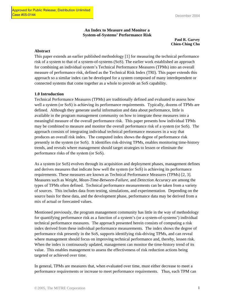
2.0 A Generalized Performance Risk Index Measure The following presents a generalized index designed to measure the performance risk of a system or a system-of-systems. The index can be applied in both contexts. It provides a numerical indicator of how well a developing system (or SoS) is progressing toward its threshold performance requirements. It serves as a yardstick that enables management to measure the “distance” the system (or SoS) is from its minimum performance thresholds and to monitor trends over time. To develop the generalized risk index, it is necessary to normalize the TPM “raw” values into a common and dimensionless scale. Figures 2 and 3 show such scales for Category A and Category B TPMs. In these figures, the left-most vertical scales reflect TPM raw values (their native units) taken from engineering measurements, tests, experiments, or prototypes. The right-



most vertical scales reflect TPM normalized values. Here, threshold values are all normalized to one. This scale transformation is done for each TPM in each category. This allows management to compare the progress of each performance measure in a common and dimensionless scale. From these normalized scales, an overall measure of the extent to which the performance of the system (or SoS) meets its threshold requirements can then be determined. Next are general formulas to derive this measure. This is followed by a computation example to illustrate the application context.

Vt1, Aj

TPMAjRaw Value Scale


t

Threshold1

TPMAj Normalized Value Scale


t

Threshold

vti, Aj = max{1 + (Vti, Aj - Vthres, Aj)/ Vthres, Aj,1},on the ith measurement date of the jth TPMin Category A

Vt3, Aj

Vt2, Aj

Vt4, Aj

vt1, Aj

vt3, Aj

vt2, Aj

vt4, Aj

Vti, Aj vti, Aj

Vthres, Aj





Figure 2. Normalized Category A TPM


Vthres, Bk

TPMBkRaw Value Scale

Threshold


Threshold

t t

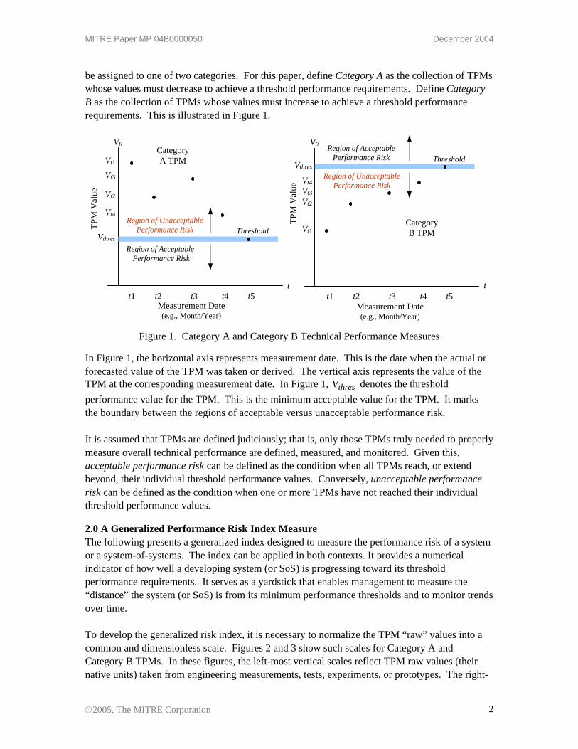
vti, Bk = min{1 - (Vthres, Bk - Vti, Bk)/ Vthres, Bk, 1}, on the ith measurement date of the kth TPM in Category B

1

TPMBkNormalized Value Scale

Vt1, Bk

Vt3, Bk Vt2, Bk

Vt4, Bk

vt1, Bk

vt3, Bkvt2, Bk

vt4, Bk

Vti, Bk vti, Bk Region of AcceptablePerformance Risk


Region of AcceptablePerformance Risk


Figure 3. Normalized Category B TPM

Mentioned previously, let Category A be the set of TPMs that need to be reduced to their threshold values. In Figure 2, let Vti, Aj be the value at time ti for the jth TPM in Category A and Vthres, Aj be the threshold value to which the jth TPM is driven. Define vti, Aj to be a normalized TPM value against its threshold as follows (assuming both Vti, Aj and Vthres, Aj are greater than 0):



vti, Aj = max{Vti, Aj, Vthres, Aj} / Vthres, Aj (i.e., threshold met if Vti, Aj < Vthres, Aj)

= max{Vti, Aj / Vthres, Aj, 1} = max{(Vthres, Aj - Vthres, Aj + Vti, Aj) / Vthres, Aj, 1}

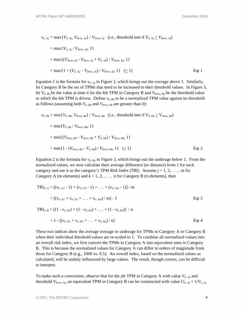
= max{1 + (Vti, Aj – Vthres, Aj) / Vthres, Aj, 1} (> 1) Eqt 1

Equation 1 is the formula for vti, Aj in Figure 2, which brings out the overage above 1. Similarly, let Category B be the set of TPMs that need to be increased to their threshold values. In Figure 3, let Vti, Bk be the value at time ti for the kth TPM in Category B and Vthres, Bk be the threshold value to which the kth TPM is driven. Define vti, Bk to be a normalized TPM value against its threshold as follows (assuming both Vti, Bk and Vthres, Bk are greater than 0): vti, Bk = min{Vti, Bk, Vthres, Bk} / Vthres, Bk (i.e., threshold met if Vti, Bk > Vthres, Bk) = min{Vti, Bk / Vthres, Bk, 1} = min{(Vthres, Bk - Vthres, Bk + Vti, Bk) / Vthres, Bk, 1}

= min{1 - (Vthres, Bk - Vti, Bk) / Vthres, Bk, 1} (< 1) Eqt 2 Equation 2 is the formula for vti, Bk in Figure 3, which brings out the underage below 1. From the normalized values, we now calculate their average difference (or distance) from 1 for each category and use it as the category’s TPM Risk Index (TRI). Assume j = 1, 2, . . . , m for Category A (m elements) and k = 1, 2, . . . , n for Category B (n elements), then TRIti, A = [(vti, A1 - 1) + (vti, A2 - 1) + . . . + (vti, Am - 1)] / m

= [(vti, A1 + vti, A2 + . . . + vti, Am) / m] - 1 Eqt 3 TRIti, B = [(1 - vti, B1) + (1 - vti, B2) + . . . + (1 - vti, Bn)] / n

= 1 - [(vti, B1 + vti, B2 + . . . + vti, Bn) / n] Eqt 4 These two indices show the average overage or underage for TPMs in Category A or Category B when their individual threshold values are re-scaled to 1. To combine all normalized values into an overall risk index, we first convert the TPMs in Category A into equivalent ones in Category B. This is because the normalized values for Category A can differ in orders of magnitude from those for Category B (e.g., 1000 vs. 0.5). An overall index, based on the normalized values as calculated, will be unduly influenced by large values. The result, though correct, can be difficult to interpret. To make such a conversion, observe that for the jth TPM in Category A with value Vti, Aj and threshold Vthres, Aj, an equivalent TPM in Category B can be constructed with value Uti, Aj = 1/Vti, Aj



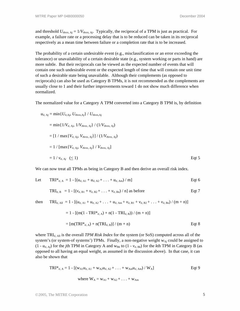
and threshold Uthres, Aj = 1/Vthres, Aj. Typically, the reciprocal of a TPM is just as practical. For example, a failure rate or a processing delay that is to be reduced can be taken in its reciprocal respectively as a mean time between failure or a completion rate that is to be increased. The probability of a certain undesirable event (e.g., misclassification or an error exceeding the tolerance) or unavailability of a certain desirable state (e.g., system working or parts in hand) are more subtle. But their reciprocals can be viewed as the expected number of events that will contain one such undesirable event or the expected length of time that will contain one unit time of such a desirable state being unavailable. Although their complements (as opposed to reciprocals) can also be used as Category B TPMs, it is not recommended as the complements are usually close to 1 and their further improvements toward 1 do not show much difference when normalized. The normalized value for a Category A TPM converted into a Category B TPM is, by definition uti, Aj = min{Uti,Aj, Uthres,Aj} / Uthres,Aj

= min{1/Vti, Aj, 1/Vthres, Aj} / (1/Vthres, Aj)

= [1 / max{Vti, Aj, Vthres, Aj}] / (1/Vthres, Aj) = 1 / [max{Vti, Aj, Vthres, Aj} / Vthres, Aj] = 1 / vti, Aj (< 1) Eqt 5 We can now treat all TPMs as being in Category B and then derive an overall risk index. Let TRI*ti, A = 1 - [(uti, A1 + uti, A2 + . . . + uti, Am) / m] Eqt 6 TRIti, B = 1 - [(vti, B1 + vti, B2 + . . . + vti, Bn) / n] as before Eqt 7 then TRIti, All = 1 - [(uti, A1 + uti, A2 + . . . + uti, Am + vti, B1 + vti, B2 + . . . + vti, Bn) / (m + n)] = 1 - [(m(1 - TRI*ti, A) + n(1 - TRIti, B)) / (m + n)] = [m(TRI*ti, A) + n(TRIti, B)] / (m + n) Eqt 8 where TRIti, All is the overall TPM Risk Index for the system (or SoS) computed across all of the system’s (or system-of systems’) TPMs. Finally, a non-negative weight wAj could be assigned to (1 - uti, Aj) for the jth TPM in Category A and wBk to (1 - vti, Bk) for the kth TPM in Category B (as opposed to all having an equal weight, as assumed in the discussion above). In that case, it can also be shown that

TRI*ti, A = 1 - [(wA1uti, A1 + wA2uti, A2 + . . . + wAmuti, Am) / WA] Eqt 9

where WA = wA1 + wA2 + . . . + wAm



TRIti, B = 1 - [(wB1vti, B1 + wB2vti, B2 + . . . + wBnvti, Bn) / WB] Eqt 10 where WB = wB1 + wB2 + . . . + wBn

and TRIti, All = [WATRI*ti, A + WBTRIti, B] / W Eqt 11

where W = WA + WB

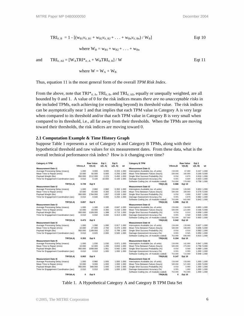
Thus, equation 11 is the most general form of the overall TPM Risk Index. From the above, note that TRI*ti, A, TRIti, B, and TRIti, All, equally or unequally weighted, are all bounded by 0 and 1. A value of 0 for the risk indices means there are no unacceptable risks in the included TPMs, each achieving (or extending beyond) its threshold value. The risk indices can be asymptotically near 1 and that implies that each TPM value in Category A is very large when compared to its threshold and/or that each TPM value in Category B is very small when compared to its threshold, i.e., all far away from their thresholds. When the TPMs are moving toward their thresholds, the risk indices are moving toward 0. 2.1 Computation Example & Time History Graph Suppose Table 1 represents a set of Category A and Category B TPMs, along with their hypothetical threshold and raw values for six measurement dates. From these data, what is the overall technical performance risk index? How is it changing over time?

Category A TPM Raw Value Eqt 1 Eqt 5 Category B TPM Raw Value Eqt 2Vthres,A V(ti,A) v(ti, A) u(ti, A) wt Vthres,B V(ti,B) v(ti, B) wt

Measurement Date t1 Measurement Date t1Average Processing Delay (msecs) 1.000 3.000 3.000 0.333 1.000 Interceptors Available (no. of units) 150.000 67.000 0.447 1.000Mean Time to Repair (mins) 10.000 50.000 5.000 0.200 1.000 Mean Time Between Failure (hours) 500.000 100.000 0.200 5.000Payload Weight (lbs) 950.000 2112.000 2.223 0.450 1.000 Single Shot Success Probability (%) 0.950 0.870 0.916 1.000Time for Engagement Coordination (sec) 0.010 0.100 10.000 0.100 1.000 Damage Assessment Accuracy (%) 0.995 0.600 0.603 1.000

Software Coding (no. of modules coded) 763.000 578.000 0.758 1.000TRI*(t1,A) 0.729 Eqt 9 TRI(t1,B) 0.586 Eqt 10 T










Software Coding (no. of modules coded) 763.000 763.000 1.000 1.000TRI*(t6,A) 0 Eqt 9 TRI(t6,B) 0 Eqt 10 T

Table 1. A Hypothetical Category A and Category B TPM Data Set



From the data in Table 1 and equations 9, 10, and 11, we can derive, for each measurement date, the TPM risk indices for the Category A and Category B TPMs, as well as for the overall TPM Risk Index. The results from these derivations are summarized in Table 2.

Measurement Date

TPM Risk Index for Category A TPMs

TRI*ti, A

Eqt 9

TPM Risk Index for Category B TPMs

TRIti, B

Eqt 10

Overall TPM Risk Index

TRIti, All

Eqt 11

t1 0.729 0.586 0.63 t2 0.657 0.399 0.478 t3 0.473 0.342 0.382 t4 0.353 0.194 0.243 t5 0.063 0.147 0.121 t6 0 0 0

Table 2. TPM Risk Index Summaries

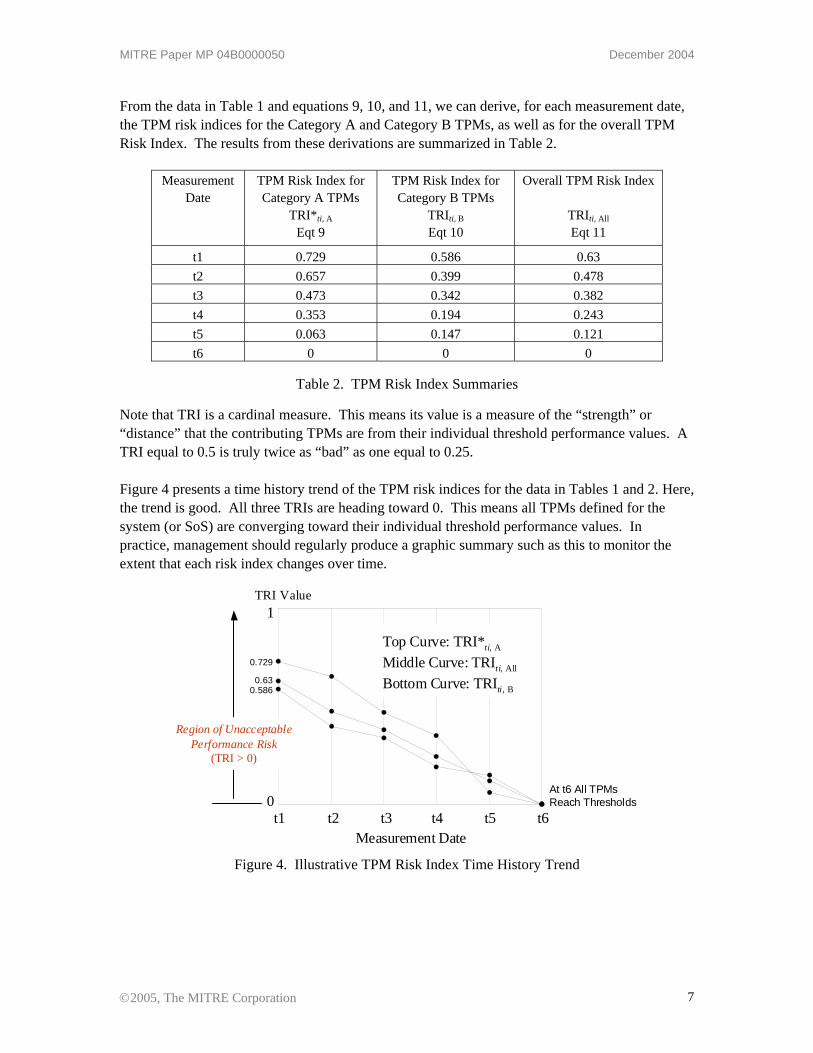
Note that TRI is a cardinal measure. This means its value is a measure of the “strength” or “distance” that the contributing TPMs are from their individual threshold performance values. A TRI equal to 0.5 is truly twice as “bad” as one equal to 0.25. Figure 4 presents a time history trend of the TPM risk indices for the data in Tables 1 and 2. Here, the trend is good. All three TRIs are heading toward 0. This means all TPMs defined for the system (or SoS) are converging toward their individual threshold performance values. In practice, management should regularly produce a graphic summary such as this to monitor the extent that each risk index changes over time.

t2t1 t3 t4 t5 t6

Top Curve: TRI*ti, A

Middle Curve: TRIti, All

Bottom Curve: TRIti, B

1

0

Measurement Date

TRI Value

0.729

0.630.586

At t6 All TPMsReach Thresholds


(TRI > 0)

Figure 4. Illustrative TPM Risk Index Time History Trend



2.2 General Equation Summary This paper provides an approach and formalism for developing an overall set of quantitative indices that measure a performance risk, as a function of a system’s (or system-of-systems’) TPMs. Below are the general equations of the three principal risk indices. Category A: TRI*ti, A = 1 - [(wA1uti, A1 + wA2uti, A2 + . . . + wAmuti, Am) / WA]

where WA = wA1 + wA2 + . . . + wAm

Category B: TRIti, B = 1 - [(wB1vti, B1 + wB2vti, B2 + . . . + wBnvti, Bn) / WB] where WB = wB1 + wB2 + . . . + wBn

Overall Risk Index:

TRIti, All = [WATRI*ti, A + WBTRIti, B] / W

where W = WA + WB

3.0 Extensions to System-of-Systems This section extends the general formulation of TRI to a system that is composed of many individual systems that, when connected, provide an overall system-of-systems capability. In this paper, we use the following definition of a system-of-systems. Definition*

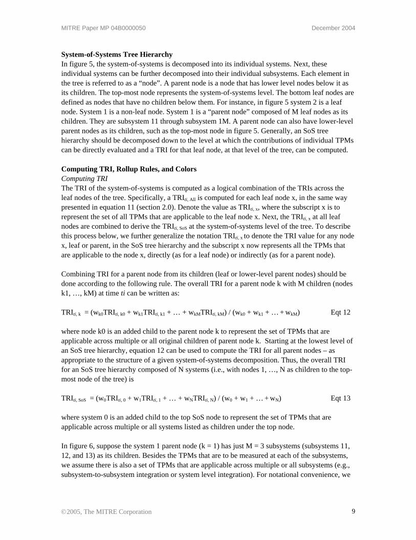
A system-of-systems (SoS) is a set or arrangement of interdependent systems that are related or connected to provide a given capability, as illustrated by figure 5. The loss of any part of the system will degrade the performance or capabilities of the whole. An example of an SoS could be interdependent information systems. While individual systems within the SoS may be developed to satisfy the peculiar needs of a given user group (like a specific Service or Agency), the information they share is so important that the loss of a single system may deprive other systems of the data needed to achieve even minimal capabilities.

System ofSystemsSystem of

Systems

System 1

System 1 System

2

System 2 System

3

System 3 System

N

System N

SubSystem11

SubSystem11 SubSystem

12


13


1M

SubSystem1M

…

…

Figure 5. An Illustrative System-of Systems Hierarchy or Decomposition Tree

* Reference: Chairman of the Joint Chiefs of Staff Manual (CJCSM 3170.01, 24 June 2003).



System-of-Systems Tree Hierarchy In figure 5, the system-of-systems is decomposed into its individual systems. Next, these individual systems can be further decomposed into their individual subsystems. Each element in the tree is referred to as a “node”. A parent node is a node that has lower level nodes below it as its children. The top-most node represents the system-of-systems level. The bottom leaf nodes are defined as nodes that have no children below them. For instance, in figure 5 system 2 is a leaf node. System 1 is a non-leaf node. System 1 is a “parent node” composed of M leaf nodes as its children. They are subsystem 11 through subsystem 1M. A parent node can also have lower-level parent nodes as its children, such as the top-most node in figure 5. Generally, an SoS tree hierarchy should be decomposed down to the level at which the contributions of individual TPMs can be directly evaluated and a TRI for that leaf node, at that level of the tree, can be computed. Computing TRI, Rollup Rules, and Colors Computing TRI The TRI of the system-of-systems is computed as a logical combination of the TRIs across the leaf nodes of the tree. Specifically, a TRIti, All is computed for each leaf node x, in the same way presented in equation 11 (section 2.0). Denote the value as TRIti, x, where the subscript x is to represent the set of all TPMs that are applicable to the leaf node x. Next, the TRIti, x at all leaf nodes are combined to derive the TRIti, SoS at the system-of-systems level of the tree. To describe this process below, we further generalize the notation TRIti, x to denote the TRI value for any node x, leaf or parent, in the SoS tree hierarchy and the subscript x now represents all the TPMs that are applicable to the node x, directly (as for a leaf node) or indirectly (as for a parent node). Combining TRI for a parent node from its children (leaf or lower-level parent nodes) should be done according to the following rule. The overall TRI for a parent node k with M children (nodes k1, …, kM) at time ti can be written as: TRIti, k = (wk0TRIti, k0 + wk1TRIti, k1 + … + wkMTRIti, kM) / (wk0 + wk1 + … + wkM) Eqt 12 where node k0 is an added child to the parent node k to represent the set of TPMs that are applicable across multiple or all original children of parent node k. Starting at the lowest level of an SoS tree hierarchy, equation 12 can be used to compute the TRI for all parent nodes – as appropriate to the structure of a given system-of-systems decomposition. Thus, the overall TRI for an SoS tree hierarchy composed of N systems (i.e., with nodes 1, …, N as children to the top-most node of the tree) is TRIti, SoS = (w0TRIti, 0 + w1TRIti, 1 + … + wNTRIti, N) / (w0 + w1 + … + wN) Eqt 13 where system 0 is an added child to the top SoS node to represent the set of TPMs that are applicable across multiple or all systems listed as children under the top node. In figure 6, suppose the system 1 parent node (k = 1) has just M = 3 subsystems (subsystems 11, 12, and 13) as its children. Besides the TPMs that are to be measured at each of the subsystems, we assume there is also a set of TPMs that are applicable across multiple or all subsystems (e.g., subsystem-to-subsystem integration or system level integration). For notational convenience, we



use subsystem 10 to denote the collection of such TPMs and use TRIti, 10 to denote the TRI value computed on those TPMs. Then, the overall TRI of system 1 at time ti is as follows:

TRIti, 1 = (w10TRIti, 10 + w11TRIti, 11 + w12TRIti, 12 + w13TRIti, 13) / (w10 + w11 + w12 + w13) Eqt 14 Clearly, if the system 1 parent node’s TRI is defined solely by its children’s TRI values then equation 14 can be simplified with w10 set equal to 0. Appendix A illustrates the computation of TRI for a system-of-systems. Other Rollup Rules Equations 12, 13, and 14 apply a weighted average rollup rule for determining the TRI values in the SoS tree hierarchy. The rule is appropriate for a parent node when its children’s performance levels are considered additive in measuring the parent node’s performance level. This implies, with their assigned weights, all children’s risk levels directly add to the parent node’s risk level. This is probably the most common rule to use in the rollup of TRI values. Other rules may also be defined and applied accordingly. For example, referring to figure 5 with M = 3, equation 12 could be rewritten according to the relationship that is considered to have among the children of the parent node system 1, as follows: (a) If subsystems 12 and 13’s performance levels are considered competing with each other as alternative to be selected in measuring the parent node’s performance level (i.e., the lowest risk level between the two will be selected to represent their singular risk level), then the min rollup rule applies: TRIti, 1 = (w10TRIti, 10 + w11TRIti, 11 + w12or13Min{TRIti, 12 , TRIti, 13}) / (w10 + w11 + w12or13) Eqt 14a where w12or13 is the weight assigned to the selected result between subsystems 12 and 13. (b) If subsystems 12 and 13’s performance levels are considered limiting to each other in contributing to the parent node’s performance level (i.e., the highest risk level between the two will be selected to represent their singular risk level), then the max rollup rule applies: TRIti, 1 = (w10TRIti, 10 + w11TRIti, 11 + w12or13Max{TRIti, 12 , TRIti, 13}) / (w10 + w11 + w12or13) Eqt 14b where w12or13 is the weight assigned to the selected result between subsystems 12 and 13. (c) If subsystems 12 and 13’s performance levels are considered in parallel redundancy in contributing to the parent node’s performance level (i.e., the net risk level of the two will be the product of their risk levels), then the multiplication rollup rule applies: TRIti, 1 = (w10TRIti, 10 + w11TRIti, 11 + w12x13[TRIti, 12 * TRIti, 13]) / (w10 + w11 + w12x13) Eqt 14c where w12x13 is the weight assigned to the product of subsystems 12 and 13’s risk levels.



(d) If subsystems 12 and 13’s performance levels are considered in serial dependency in measuring the parent node’s performance level (i.e., their risk levels will aggravate each other to produce a combined risk level of the two), then the complementary multiplication rollup rule applies: TRIti, 1 = (w10TRIti, 10 + w11TRIti, 11 + w12x13[1 – (1-TRIti, 12) *(1-TRIti, 13)]) / (w10 + w11 + w12x13) Eqt 14d

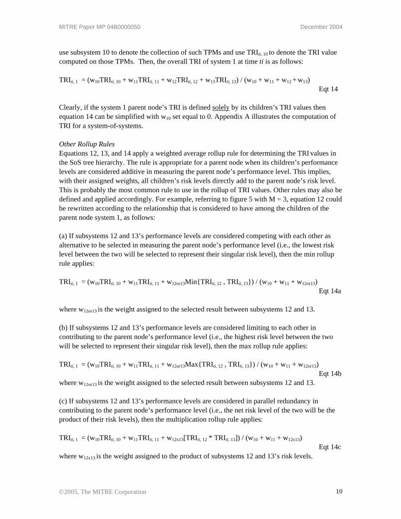
where w12x13 is the weight assigned to the complementary product of subsystems 12 and 13’s risk levels. Additional rollup rules could be defined to meet other specific measuring needs. Conceptually, all these rollup rules can be expressed for any general node in an SoS tree hierarchy. But since a different combination of rules could apply to different nodes, such a general expression becomes difficult. Color Determinations Since the TRI metric is bounded between zero and unity it is convenient to express the TRI as a color, in addition to its computed numerical value. Figure 6 presents a set of colors that can be applied to each node of the tree hierarchy to provide a quick visual communication of the TRI value and status of the SoS. Such a visual display can be very helpful to program managers and decision-makers. The color range in figure 6 can also be adjusted to reflect the choice of color boundaries by management.


Systems

Defense

1System

DefenseSystem

1

DefensSystem

e

2

DefenseSystem

2

DefensSystem

e

3

DefenseSystem

3

WeaponSubSystem

11

WeaponSubSystem

11

TrackerSubSystem

13

TrackerSubSystem

13

Sensor ManageSubSystem

1

r

4

Sensor ManagerSubSystem

14

CommsSubSystem

15

CommsSubSystem

15

DefensSystem

e

4

DefenseSystem

4

SensorSubSystem

12

SensorSubSystem

12

TRI = 0.60 TRI = 0.65 TRI = 0.70TRI = 0.497

TRI = 0.549

DefensSystem

e

0

DefenseSystem

0

TRI = 0.30

SubSystem10

SubSystem10

TRI = 0.35

TRI = 0.483 TRI = 0.646 TRI = 0.303 TRI = 0.472 TRI = 0.726

TRI Values at Time t1

Orange

Orange Orange Orange Red

Red

Orange

Orange Orange OrangeYellow

Yellow

RED

YELLOW

GREEN

1

< 2/3

< 1/3

= 0

TRI Color TRI Score

ORANGE

> 0

RED

YELLOW

GREEN

1

< 2/3

< 1/3

= 0

TRI Color TRI Score

ORANGE

> 0


Systems

DefensSystem

e

1

DefenseSystem

1

DefensSystem

e

2

DefenseSystem

2

DefensSystem

e

3

DefenseSystem

3

WeaponSubSystem

11

WeaponSubSystem

11

TrackerSubSystem

13

TrackerSubSystem

13


1

r

4


14

CommsSubSystem

15

CommsSubSystem

15

DefensSystem

e

4

DefenseSystem

4

SensorSubSystem

12

SensorSubSystem

12

TRI = 0.60 TRI = 0.65 TRI = 0.70TRI = 0.497

TRI = 0.549

DefensSystem

e

0

DefenseSystem

0

TRI = 0.30

SubSystem10

SubSystem10

TRI = 0.35



Orange


Red

Orange


Yellow

RED

YELLOW

GREEN

1

< 2/3

< 1/3

= 0

TRI Color TRI Score

ORANGE

> 0

RED

YELLOW

GREEN

1

< 2/3

< 1/3

= 0

TRI Color TRI Score

ORANGE

> 0

Figure 6. An Illustrative SoS Hierarchy, TRI Values, and Associated Colors



4.0 Summary To conclude, key features of the approach presented in the paper are summarized as follows:

• Provides Integrated Measures of Technical Performance: This approach provides management with a way to transform the typically dozen or more TPMs into common measurement scales. From this, all TPMs may then be integrated and combined in a way that provides management with meaningful and comparative measures of the overall performance risk of the system (or SoS), at any measurement time t.

• Measures Technical Performance as a Function of the Physical Parameters of the TPMs: This approach operates on actual or predicted values from engineering measurements, tests, experiments, or prototypes. As such, the physical parameters that characterize the TPMs provide the basis for deriving the TPM risk indices.

• Measures the Degree of Risk and Monitors Change over Time: The computed TPM risk indices show the degree of performance risk that presently exists in the system (or SoS), supports the identification and ranking of risk-driving TPMs, and can reveal where management should focus on improving technical performance and, thereby, lessen risk. If the indices are continuously updated, then management can monitor the time-history trends of their values to assess the effectiveness of risk reduction actions being targeted or achieved over time.

Lastly, note that the TRI calculation so far in this paper assumes the TPMs’ threshold values as the goals that the technical performance is driven to reach. The resulting index value measures the distance between the achieved technical performance levels and those considered minimally acceptable. Conceptually, one can use the TPMs’ objective values, the desirable but more demanding technical performance levels, to replace the threshold values in the TRI calculation. The result will be an index to measure the distance between the achieved levels and those considered desirable.

References [1] An Index to Measure a System’s Performance Risk, The Acquisition Review Quarterly (ARQ), Vol. 10, No. 2, Spring 2003.

[2] Risk Management Guide for DoD Acquisition, 5th Ed, Department of Defense, Defense Acquisition University (DAU), DAU Press, Fort Belvoir, VA, June 2002.

[3] Blanchard, B. S., and W. J. Fabrycky. 1990. Systems Engineering and Analysis, 2nd ed. Englewood Cliffs, New Jersey: Prentice-Hall, Inc.



About the Authors… Paul R. Garvey is Chief Scientist, and a Director, for the Center for Acquisition and Systems Analysis at The MITRE Corporation. Mr. Garvey is internationally recognized and widely published in the application of decision analytic methods to problems in systems engineering risk management. His articles in this area have appeared in numerous peer‐reviewed journals, technical books, and recently in John Wiley & Son’s Encyclopedia of Electrical and Electronics Engineering. Mr. Garvey authored the textbook “Probability Methods for Cost Uncertainty Analysis: A Systems Engineering Perspective”, published by Marcel Dekker, Inc., New York, NY. Mr. Garvey completed his undergraduate and graduate degrees in mathematics and applied mathematics at Boston College and Northeastern University, where he was a member of the adjunct faculty in the Department of Mathematics.

Chien‐Ching Cho is Principal Staff in the Economic and Decision Analysis Center, a department within the Center for Acquisition and Systems Analysis, at The MITRE Corporation. Dr. Cho has significant experience in applying operations research methods and statistical analysis techniques to a wide variety of systems engineering and analysis problems. Dr. Cho received his Ph.D. from the University of Wisconsin (Madison) in Operations Research with a minor in Statistics.

The authors would like to acknowledge and thank Mr. Stephen Myers, Principal Professional Staff, at the Johns Hopkins University Applied Physics Laboratory (JHU/APL) for his contributions to and review of the computational example in the Appendix of this paper.





Appendix A

Computing a System-of-Systems’ Technical Performance Risk Index (TRI)

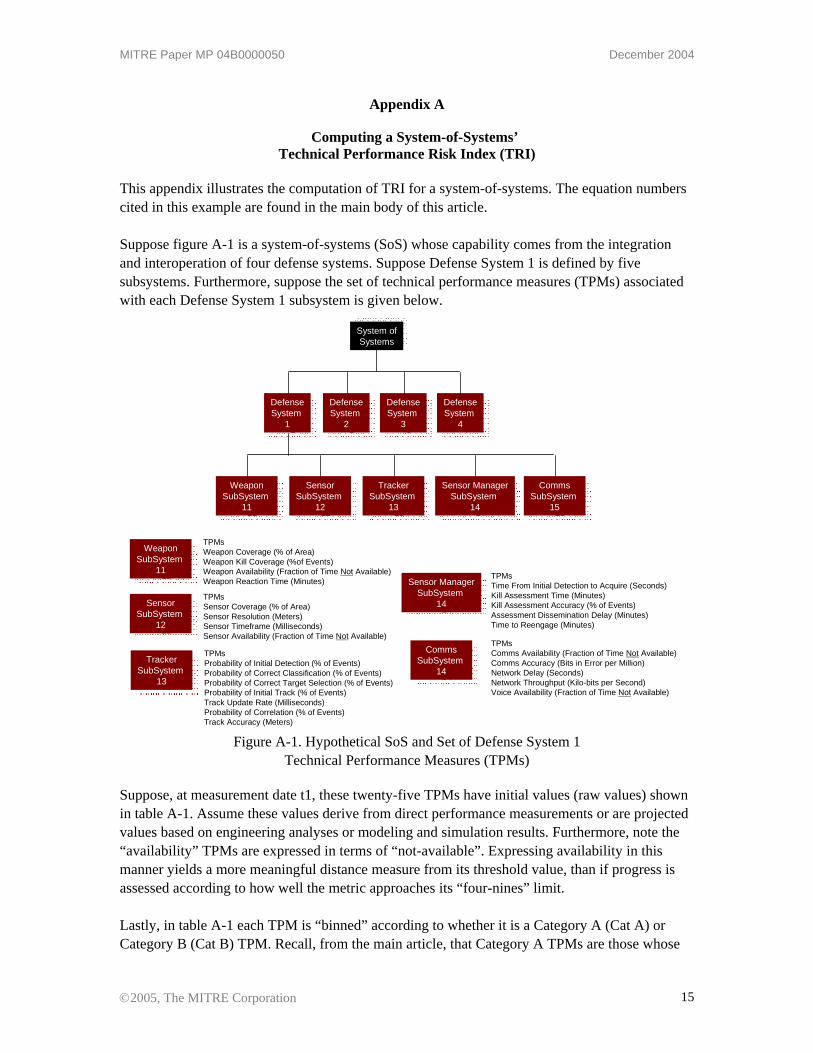
This appendix illustrates the computation of TRI for a system-of-systems. The equation numbers cited in this example are found in the main body of this article. Suppose figure A-1 is a system-of-systems (SoS) whose capability comes from the integration and interoperation of four defense systems. Suppose Defense System 1 is defined by five subsystems. Furthermore, suppose the set of technical performance measures (TPMs) associated with each Defense System 1 subsystem is given below.


Systems

Defense

1System

DefenseSystem

1

DefensSystem

e

2

DefenseSystem

2

DefensSystem

e

3

DefenseSystem

3

WeaponSubSystem

11

WeaponSubSystem

11

TrackerSubSystem

13

TrackerSubSystem

13


1

r

4


14

CommsSubSystem

15

CommsSubSystem

15

DefensSystem

e

4

DefenseSystem

4

WeaponSubSystem

11

WeaponSubSystem

11

TPMsWeapon Coverage (% of Area)Weapon Kill Coverage (%of Events)Weapon Availability (Fraction of Time Not Available)Weapon Reaction Time (Minutes)

SensorSubSystem

12

SensorSubSystem

12

TPMsSensor Coverage (% of Area)Sensor Resolution (Meters)Sensor Timeframe (Milliseconds)Sensor Availability (Fraction of Time Not Available)

SensorSubSystem

12

SensorSubSystem

12

TrackerSubSystem

13

TrackerSubSystem

13

TPMsProbability of Initial Detection (% of Events)Probability of Correct Classification (% of Events)Probability of Correct Target Selection (% of Events)Probability of Initial Track (% of Events)Track Update Rate (Milliseconds)Probability of Correlation (% of Events)Track Accuracy (Meters)


1

r

4


14

TPMsTime From Initial Detection to Acquire (Seconds)Kill Assessment Time (Minutes)Kill Assessment Accuracy (% of Events)Assessment Dissemination Delay (Minutes)Time to Reengage (Minutes)

CommsSubSystem

14

CommsSubSystem

14

TPMsComms Availability (Fraction of Time Not Available)Comms Accuracy (Bits in Error per Million)Network Delay (Seconds)Network Throughput (Kilo-bits per Second)Voice Availability (Fraction of Time Not Available)

Figure A-1. Hypothetical SoS and Set of Defense System 1

Technical Performance Measures (TPMs)

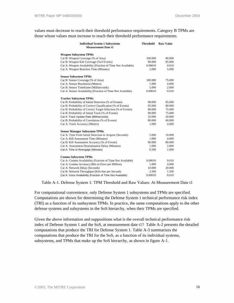
Suppose, at measurement date t1, these twenty-five TPMs have initial values (raw values) shown in table A-1. Assume these values derive from direct performance measurements or are projected values based on engineering analyses or modeling and simulation results. Furthermore, note the “availability” TPMs are expressed in terms of “not-available”. Expressing availability in this manner yields a more meaningful distance measure from its threshold value, than if progress is assessed according to how well the metric approaches its “four-nines” limit. Lastly, in table A-1 each TPM is “binned” according to whether it is a Category A (Cat A) or Category B (Cat B) TPM. Recall, from the main article, that Category A TPMs are those whose



values must decrease to reach their threshold performance requirements. Category B TPMs are those whose values must increase to reach their threshold performance requirements.

Individual System 1 Subsystems Threshold Raw ValueMeasurement Date t1

Weapon Subsystem TPMsCat B: Weapon Coverage (% of Area) 100.000 80.000Cat B: Weapon Kill Coverage (%of Events) 99.000 85.000Cat A: Weapon Availability (Fraction of Time Not Available) 0.00010 0.010Cat A: Weapon Reaction Time (Minutes) 2.000 5.000

Sensor Subsystem TPMsCat B: Sensor Coverage (% of Area) 100.000 75.000Cat A: Sensor Resolution (Meters) 1.000 4.000Cat B: Sensor Timeframe (Milliseconds) 5.000 2.000Cat A: Sensor Availability (Fraction of Time Not Available) 0.00010 0.010

Tracker Subsystem TPMsCat B: Probability of Initial Detection (% of Events) 98.000 85.000Cat B: Probability of Correct Classification (% of Events) 95.000 80.000Cat B: Probability of Correct Target Selection (% of Events) 90.000 75.000Cat B: Probability of Initial Track (% of Events) 90.000 75.000Cat A: Track Update Rate (Milliseconds) 10.000 20.000Cat B: Probability of Correlation (% of Events) 80.000 60.000Cat A: Track Accuracy (Meters) 1.000 4.000

Sensor Manager Subsystem TPMsCat A: Time From Initial Detection to Acquire (Seconds) 5.000 10.000Cat A: Kill Assessment Time (Minutes) 1.000 4.000Cat B: Kill Assessment Accuracy (% of Events) 90.000 80.000Cat A: Assessment Dissemination Delay (Minutes) 1.000 2.000Cat A: Time to Reengage (Minutes) 0.500 1.000

Comms Subsystem TPMsCat A: Comms Availability (Fraction of Time Not Available) 0.00010 0.010Cat A: Comms Accuracy (Bits in Error per Million) 1.000 4.000Cat A: Network Delay (Seconds) 10.000 20.000Cat B: Network Throughput (Kilo-bits per Second) 2.500 1.500Cat A: Voice Availability (Fraction of Time Not Available) 0.00010 0.010

Table A-1. Defense System 1: TPM Threshold and Raw Values: At Measurement Date t1

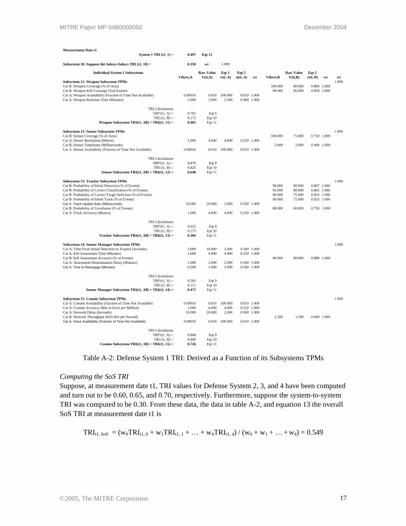
For computational convenience, only Defense System 1 subsystems and TPMs are specified. Computations are shown for determining the Defense System 1 technical performance risk index (TRI) as a function of its susbsystem TPMs. In practice, the same computations apply to the other defense systems and subsystems in the SoS hierarchy, when their TPMs are specified. Given the above information and suppositions what is the overall technical performance risk index of Defense System 1 and the SoS, at measurement date t1? Table A-2 presents the detailed computations that produce the TRI for Defense System 1. Table A-3 summarizes the computations that produce the TRI for the SoS, as a function of its individual systems, subsystems, and TPMs that make up the SoS hierarchy, as shown in figure A-1.



Measurement Date t1System 1 TRI (t1, 1) = 0.497 Eqt 12

Subsystem 10: Suppose the Subsys-Subsys TRI (t1, 10) = 0.350 wt 1.000

Individual System 1 Subsystems Raw Value Eqt 1 Eqt 5 Raw Value Eqt 2Vthres,A V(ti,A) v(ti, A) u(ti, A) wt Vthres,B V(ti,B) v(ti, B) wt wt

Subsystem 11: Weapon Subsystem TPMs 1.000Cat B: Weapon Coverage (% of Area) 100.000 80.000 0.800 1.000Cat B: Weapon Kill Coverage (%of Events) 99.000 85.000 0.859 1.000Cat A: Weapon Availability (Fraction of Time Not Available) 0.00010 0.010 100.000 0.010 1.000 Cat A: Weapon Reaction Time (Minutes) 2.000 5.000 2.500 0.400 1.000

TRI Calculations

TRI*(t1, A) = 0.795 Eqt 9TRI (t1, B) = 0.171 Eqt 10

Weapon Subsystem TRI(t1, All) = TRI(t1, 11) = 0.483 Eqt 11

Subsystem 12: Sensor Subsystem TPMs 1.000Cat B: Sensor Coverage (% of Area) 100.000 75.000 0.750 1.000Cat A: Sensor Resolution (Meters) 1.000 4.000 4.000 0.250 1.000Cat B: Sensor Timeframe (Milliseconds) 5.000 2.000 0.400 1.000Cat A: Sensor Availability (Fraction of Time Not Available) 0.00010 0.010 100.000 0.010 1.000

TRI Calculations


Sensor Subsystem TRI(t1, All) = TRI(t1, 12) = 0.648 Eqt 11

Subsystem 13: Tracker Subsystem TPMs 1.000Cat B: Probability of Initial Detection (% of Events) 98.000 85.000 0.867 1.000Cat B: Probability of Correct Classification (% of Events) 95.000 80.000 0.842 1.000Cat B: Probability of Correct Target Selection (% of Events) 90.000 75.000 0.833 1.000Cat B: Probability of Initial Track (% of Events) 90.000 75.000 0.833 1.000Cat A: Track Update Rate (Milliseconds) 10.000 20.000 2.000 0.500 1.000Cat B: Probability of Correlation (% of Events) 80.000 60.000 0.750 1.000Cat A: Track Accuracy (Meters) 1.000 4.000 4.000 0.250 1.000

TRI Calculations


Tracker Subsystem TRI(t1, All) = TRI(t1, 13) = 0.304 Eqt 11

Subsystem 14: Sensor Manager Subsystem TPMs 1.000Cat A: Time From Initial Detection to Acquire (Seconds) 5.000 10.000 2.000 0.500 1.000 Cat A: Kill Assessment Time (Minutes) 1.000 4.000 4.000 0.250 1.000 Cat B: Kill Assessment Accuracy (% of Events) 90.000 80.000 0.889 1.000Cat A: Assessment Dissemination Delay (Minutes) 1.000 2.000 2.000 0.500 1.000 Cat A: Time to Reengage (Minutes) 0.500 1.000 2.000 0.500 1.000

TRI Calculations


Sensor Manager Subsystem TRI(t1, All) = TRI(t1, 14) = 0.473 Eqt 11

Subsystem 15: Comms Subsystem TPMs 1.000Cat A: Comms Availability (Fraction of Time Not Available) 0.00010 0.010 100.000 0.010 1.000 Cat A: Comms Accuracy (Bits in Error per Million) 1.000 4.000 4.000 0.250 1.000 Cat A: Network Delay (Seconds) 10.000 20.000 2.000 0.500 1.000 Cat B: Network Throughput (Kilo-bits per Second) 2.500 1.500 0.600 1.000Cat A: Voice Availability (Fraction of Time Not Available) 0.00010 0.010 100.000 0.010 1.000

TRI Calculations


Comms Subsystem TRI(t1, All) = TRI(t1, 15) = 0.726 Eqt 11 Table A-2: Defense System 1 TRI: Derived as a Function of its Subsystems TPMs

Computing the SoS TRI Suppose, at measurement date t1, TRI values for Defense System 2, 3, and 4 have been computed and turn out to be 0.60, 0.65, and 0.70, respectively. Furthermore, suppose the system-to-system TRI was computed to be 0.30. From these data, the data in table A-2, and equation 13 the overall SoS TRI at measurement date t1 is

TRIt1, SoS = (w0TRIt1, 0 + w1TRIt1, 1 + … + w4TRIt1, 4) / (w0 + w1 + … + w4) = 0.549



Measurement Date t1 TRI Weight (wt)

System of Systems (SoS) TRI (t1, SoS) = 0.549 Eqt 13

System 0 Suppose the System-System TRI (t1, 0) = 0.300 1.000

Individual Systems Within The SoS

System 1Computed System 1 TRI(t1, 1) = 0.497 1.000

System 2 Suppose System 2 TRI(t1, 2) = 0.600 1.000



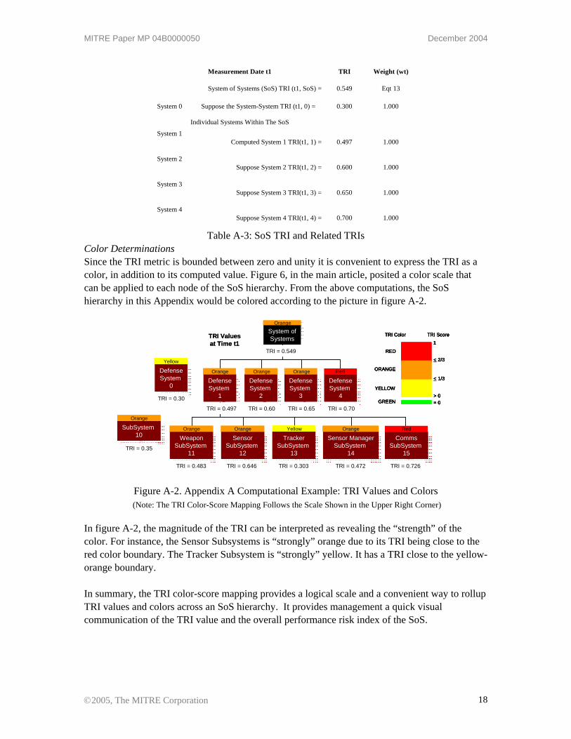
Table A-3: SoS TRI and Related TRIs Color Determinations Since the TRI metric is bounded between zero and unity it is convenient to express the TRI as a color, in addition to its computed value. Figure 6, in the main article, posited a color scale that can be applied to each node of the SoS hierarchy. From the above computations, the SoS hierarchy in this Appendix would be colored according to the picture in figure A-2.


Systems

Defense

1System

DefenseSystem

1

DefensSystem

e

2

DefenseSystem

2

DefensSystem

e

3

DefenseSystem

3

WeaponSubSystem

11

WeaponSubSystem

11

TrackerSubSystem

13

TrackerSubSystem

13


1

r

4


14

CommsSubSystem

15

CommsSubSystem

15

DefensSystem

e

4

DefenseSystem

4

SensorSubSystem

12

SensorSubSystem

12

TRI = 0.60 TRI = 0.65 TRI = 0.70TRI = 0.497

TRI = 0.549

DefensSystem

e

0

DefenseSystem

0

TRI = 0.30

SubSystem10

SubSystem10

TRI = 0.35



Orange


Red

Orange


Yellow

RED

YELLOW

GREEN

1

< 2/3

< 1/3

= 0

TRI Color TRI Score

ORANGE

> 0

RED

YELLOW

GREEN

1

< 2/3

< 1/3

= 0

TRI Color TRI Score

ORANGE

> 0


Systems

DefensSystem

e

1

DefenseSystem

1

DefensSystem

e

2

DefenseSystem

2

DefensSystem

e

3

DefenseSystem

3

WeaponSubSystem

11

WeaponSubSystem

11

TrackerSubSystem

13

TrackerSubSystem

13


1

r

4


14

CommsSubSystem

15

CommsSubSystem

15

DefensSystem

e

4

DefenseSystem

4

SensorSubSystem

12

SensorSubSystem

12

TRI = 0.60 TRI = 0.65 TRI = 0.70TRI = 0.497

TRI = 0.549

DefensSystem

e

0

DefenseSystem

0

TRI = 0.30

SubSystem10

SubSystem10

TRI = 0.35



Orange


Red

Orange


Yellow

RED

YELLOW

GREEN

1

< 2/3

< 1/3

= 0

TRI Color TRI Score

ORANGE

> 0

RED

YELLOW

GREEN

1

< 2/3

< 1/3

= 0

TRI Color TRI Score

ORANGE

> 0

Figure A-2. Appendix A Computational Example: TRI Values and Colors (Note: The TRI Color-Score Mapping Follows the Scale Shown in the Upper Right Corner)

In figure A-2, the magnitude of the TRI can be interpreted as revealing the “strength” of the color. For instance, the Sensor Subsystems is “strongly” orange due to its TRI being close to the red color boundary. The Tracker Subsystem is “strongly” yellow. It has a TRI close to the yellow-orange boundary. In summary, the TRI color-score mapping provides a logical scale and a convenient way to rollup TRI values and colors across an SoS hierarchy. It provides management a quick visual communication of the TRI value and the overall performance risk index of the SoS.


Documents

An Index to Measure and Monitor a System of Systems