An Introduction to

Algebraic, Scientific, and Statistical Computing:

an Open Source Approach Using Sage

William A. Stein

April 4, 2008

Abstract

This is an undergraduate textbook about algebraic, scientific, and statisticalcomputing using the free open source mathematical software system Sage.

Contents

1 Computing with Sage 61.1 Installing and Using Sage . . . . . . . . . . . . . . . . . . . . . . 6

1.1.1 Installing Sage . . . . . . . . . . . . . . . . . . . . . . . . 61.1.2 The command line and the notebook . . . . . . . . . . . . 81.1.3 Loading and saving variables and sessions . . . . . . . . . 13

1.2 Python: the Language of Sage . . . . . . . . . . . . . . . . . . . . 151.2.1 Lists, Tuples, Strings, Dictionaries and Sets . . . . . . . . 151.2.2 Control Flow, Errors and Exceptions . . . . . . . . . . . . 241.2.3 Classes and Inheritence . . . . . . . . . . . . . . . . . . . 24

1.3 Cython: Compiled Python . . . . . . . . . . . . . . . . . . . . . . 241.3.1 The Cython project . . . . . . . . . . . . . . . . . . . . . 241.3.2 How to use Cython: command line, notebook . . . . . . . 24

1.4 Debugging and Profiling . . . . . . . . . . . . . . . . . . . . . . . 251.4.1 Using Print Statements . . . . . . . . . . . . . . . . . . . 261.4.2 Debugging Python using pdb . . . . . . . . . . . . . . . . 261.4.3 Debugging Cython using gdb . . . . . . . . . . . . . . . . 26

1.5 Source Control Management . . . . . . . . . . . . . . . . . . . . . 261.5.1 Distributed versus Centralized . . . . . . . . . . . . . . . 261.5.2 Mercurial . . . . . . . . . . . . . . . . . . . . . . . . . . . 26

1.6 Using Mathematica, Matlab, Maple, etc., from Sage . . . . . . . 26

2 Algebraic Computing 282.1 Groups, Rings and Fields . . . . . . . . . . . . . . . . . . . . . . 28

2.1.1 Groups . . . . . . . . . . . . . . . . . . . . . . . . . . . . 282.1.2 Rings . . . . . . . . . . . . . . . . . . . . . . . . . . . . . 282.1.3 Fields . . . . . . . . . . . . . . . . . . . . . . . . . . . . . 28

2.2 Number Theory . . . . . . . . . . . . . . . . . . . . . . . . . . . . 282.2.1 Prime numbers and integer factorization . . . . . . . . . . 282.2.2 Elliptic curves . . . . . . . . . . . . . . . . . . . . . . . . 282.2.3 Public-key cryptography: Diffie-Hellman, RSA, and El-

liptic curve . . . . . . . . . . . . . . . . . . . . . . . . . . 282.3 Linear Algebra . . . . . . . . . . . . . . . . . . . . . . . . . . . . 28

2.3.1 Matrix arithmetic and echelon form . . . . . . . . . . . . 282.3.2 Vector spaces and free modules . . . . . . . . . . . . . . . 29

1

2.3.3 Solving linear systems . . . . . . . . . . . . . . . . . . . . 292.4 Systems of polynomial equations . . . . . . . . . . . . . . . . . . 292.5 Graph Theory . . . . . . . . . . . . . . . . . . . . . . . . . . . . . 29

2.5.1 Creating graphs and plotting them . . . . . . . . . . . . . 292.5.2 Computing automorphisms and isomorphisms . . . . . . . 292.5.3 The genus and other invariants . . . . . . . . . . . . . . . 29

3 Scientific Computing 303.1 Floating Point Numbers . . . . . . . . . . . . . . . . . . . . . . . 31

3.1.1 Machine precision floating point numbers . . . . . . . . . 313.1.2 Arbitrary precision floating point numbers . . . . . . . . . 31

3.2 Interval arithmetic . . . . . . . . . . . . . . . . . . . . . . . . . . 313.3 Root Finding and Optimization . . . . . . . . . . . . . . . . . . . 31

3.3.1 Single variable: max, min, roots, rational root isolation . 313.3.2 Multivariable: local max, min, roots . . . . . . . . . . . . 31

3.4 NumericalSolution of Linear Systems . . . . . . . . . . . . . . . . 313.4.1 Solving linear systems using LU factorization . . . . . . . 313.4.2 Solving linear systems iteratively . . . . . . . . . . . . . . 313.4.3 Eigenvalues and eigenvectors . . . . . . . . . . . . . . . . 31

3.5 Symbolic Calculus . . . . . . . . . . . . . . . . . . . . . . . . . . 313.5.1 Symbolic Differentiation and integration . . . . . . . . . . 313.5.2 Symbolic Limits and Taylor series . . . . . . . . . . . . . 313.5.3 Numerical Integration . . . . . . . . . . . . . . . . . . . . 31

4 Statistical Computing 324.1 Introduction to R and Scipy.stats . . . . . . . . . . . . . . . . . . 32

4.1.1 The R System for Statistical Computing . . . . . . . . . . 324.1.2 The Scipy.stats Python Library . . . . . . . . . . . . . . . 32

4.2 Descriptive Statistics . . . . . . . . . . . . . . . . . . . . . . . . . 324.2.1 Mean, standard deviation, etc. . . . . . . . . . . . . . . . 32

4.3 Inferential Statistics . . . . . . . . . . . . . . . . . . . . . . . . . 324.3.1 Simple Inference . . . . . . . . . . . . . . . . . . . . . . . 324.3.2 Conditional Inference . . . . . . . . . . . . . . . . . . . . 32

4.4 Regression . . . . . . . . . . . . . . . . . . . . . . . . . . . . . . . 324.4.1 Linear regression . . . . . . . . . . . . . . . . . . . . . . . 324.4.2 Logistic regression . . . . . . . . . . . . . . . . . . . . . . 32

2

Preface

This is an undergraduate textbook about Sage, which is a free open sourcecomputational environment for the mathematical sciences. Sage includes op-timized full-featured implementations of algorithms for computations in puremathematics, applied mathematics, and statistics.

I started the Sage project in late 2004 as a project to provide a viableopen source free alternative to the Magma computer algebra system [BCP97].My main motivation for this was frustration with not being allowed to easilychange or understand the internals of Magma, worry about the longterm futureof Magma, and concern that students and researchers in number theory couldnot easily use the Magma-based tools that I had spent six hard years developing.I started Sage as a new project instead of switching from Magma to an existingopen source system, since the only free open source software for number theoryis PARI [ABC+], whose functionality was far behind that of Magma in severalareas of interest to me (exact linear algebra and arithmetic of algebraic curves).Since PARI development moves slowly (or I am a very impatient person!), Ididn’t think it was likely this would change in the near future. PARI is asuperb program – it just doesn’t meet my needs, and has design constraintsthat make it impossible to modify so that it does so.

The Sage mathematical software system takes a fresh approach to mathemat-ical software development and architecture. For instance, one major distinctionbetween Sage and older systems is that Sage uses a standard language. Maple,Mathematica, Magma, Matlab, PARI, Gap, etc., all use their own special pur-poses language written just for mathematics. In sharp contrast, one works withSage using Python, which is one of the world’s most popular general purposescripting languages. This has some drawbacks, e.g., some mathematical expres-sions can be more difficult to express in Python than in Mathematica (say), butthe overall pros greatly outweigh the cons. By using Python, one can use al-most anything ever written in Python directly in Sage. And there is much usefulPython code out there that adddresses a wide range of application areas1:

• “Python is fast enough for our site and allows us to produce maintainablefeatures in record times, with a minimum of developers,” said Cuong Do,Software Architect, YouTube.com.

1These quotes came from the Python website.

3

• “Google has made no secret of the fact they use Python a lot for a numberof internal projects. Even knowing that, once I was an employee, I wasamazed at how much Python code there actually is in the Google sourcecode system.”, said Guido van Rossum, Google, creator of Python.

• “Python plays a key role in our production pipeline. Without it a projectthe size of Star Wars: Episode II would have been very difficult to pulloff. From crowd rendering to batch processing to compositing, Pythonbinds all things together,” said Tommy Burnette, Senior Technical Direc-tor, Industrial Light & Magic.

Instead of writing many of the core libraries from scratch like Maple, Math-ematica, Magma, Gap, PARI, Singular, and Matlab did, in Sage I assembledtogether the best open source software out there, and built on it, always makingcertain that the complete system was easily buildable from source on a reason-able range of computers. I was able to do this to a large extent with Sagebecause of fortuitous timing: the components were out there and mature, theircode is stable, and their copyright licences are clear and compatible (none of thiswas the case when the afformentioned math software was started). Of coursethere are drawbacks to this approach. Some of the upstream libraries can bedifficult to understand, are written in a range of languages, and have differentconventions than Sage. By strongly encouraging good relations between theSage project and the projects that create many of the components of Sage, weturn these weakness into strengths.

A wide and vibrant community of developers and users have become involvedwith Sage. Due to the broad interests of this large community of developers,Sage has grown into a project with the following specific goal:

Mission Statement: Provide a viable free open source alternativeto Magma, Maple, Mathematica, and Matlab.

Among many other things, this mission statement implies that in order to suc-ceed Sage should have a graphical user interface, 2D and 3D graphics, supportfor statistical and numerical computation, and much more.

Sage is starting to be recognized worldwide as a useful tool in mathematicseducation and research. Sage won first prize in the Scientific Category of the2007 Trophees du Libre.

4

The Sage development model has also matured. There are now regularreleases of Sage about once every two weeks, and all code that goes into Sageis peer reviewed.

Sage has also received generous financial support from mathematics insti-tutions (including the Clay Mathematics Institute, MSRI, PIMS, and IPAM),universities such as University of Washington and University of Bristol, andfrom the National Science Foundation, the Department of Defense, and Mi-crosoft Corporation.

Exercise 0.1.

1. Make a list of 5 free open source programs you have used.

2. For each program, write down a corresponding commercial program, if itexists.

3. List some of the pros and cons from your perspective of the free programversus the commercial version.

Acknowledgements: Many people gave me feedback on this book includingFernando Perez, Timothy Clemans, Hector Villafuerte, ...

5

Chapter 1

Computing with Sage

1.1 Installing and Using Sage

1.1.1 Installing Sage

You are strongly encouraged to follow along with all examples in this book. GetSage up and running now! Try out everything, modify things, experiment, lookunder the hood, and do all the exercises!

The website http://sagemath.org/lists.html lists the two mainSage mailing list: sage-support and sage-devel. The first is for all questionsabout using and installing Sage, and for bug reports. The second is for discus-sion related directly to modifying and improving Sage. Join these lists; notethat you will likely want to select daily digest for message deliver, so that youreceive one email a day instead of 50!

6

If you find a bug in Sage, we want to know about it! Send an email tosage-support describing the bug in as much detail as you can.

The exact details for installing Sage will change over time. The followingbriefly describes the situation in April 2008; for more details see the Sage in-stallation guide.

You install Sage on any computer either by extracting a pre-compiled binaryor building from source.

To install a binary, download the binary (either a .tar.gz file, a .dmg file,or a .7z file) from http://sagemath.org, extract the file, and following thedirections in the README.txt file. In most cases, you can simply put theextracted sage-x.y.z directory somewhere, and run Sage from there.

Installing Sage on Microsoft Windows currently involves installing theVMware player program, then running a virtual machine. This will likely changesignificantly within a year.

Currently you can only build Sage from source on Linux and OS X (or onWindows in a Linux virtual machine). To build from source, which will takeover an hour, first download sage-x.y.z.tar from http://sagemath.org/download.html. Once you have downloaded Sage, extract the “tarball”as follows:

$ tar xvf sage-x.y.z.tar

Then run the make command in the sage-x.y.z directory:$ cd sage-x.y.z$ make... 137600 lines of output ...real 102m57.600suser 71m10.115ssys 14m56.116sTo install gap, gp, singular, etc., scriptsin a standard bin directory, start sage andtype something like

sage: install_scripts(’/usr/local/bin’)at the SAGE command prompt.

SAGE build/upgrade complete!

The above should work if you have gcc, g++, make, and a few other prerequi-sites installed (Sage includes almost all depedencies), and are using a supportedarchitecture and operating system. An advantage of building from source is thatif you can build from source, then you can change absolutely any part of Sageand use the modified version. If you run into trouble, email sage-support.

Exercise 1.1. Install Sage on a computer.

7

1.1.2 The command line and the notebook

The command line and the Sage notebook provide two complementary waysfor you to interactively work with Sage. The command line provides a simpleand powerful way to type Sage commands. The notebook provides a modernAJAX web-browser based graphical interface to Sage. Both the notebook andcommand line have advantages and disadvantages, and you will want to becomefamiliar with each. For example, the notebook is better for graphics, whereasthe command line is better for debugging and profiling code (see Section 1.4).

Technical Note 1.2. The Sage command line is a customized version of theincredible IPython interactive shell by Fernando Perez et al. [PG07]. The Sagenotebook is a Python/Javascript AJAX application built by the author and T.Boothby, T. Clemans, A. Clemesha, B. Moretti, Y. Qiang and D. Raymer; isuses Twisted [Twi], Pexpect [Pex], and jQuery [jQu].

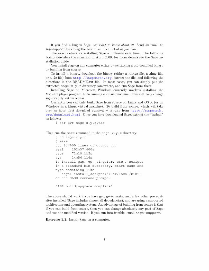
In Linux or OS X, start the command line by typing ./sage in the direc-tory where you installed Sage, or just type sage if the Sage install directorysage-x.y.z is in your PATH. In Windows, after starting the Sage vmwareimage, type sage at the login prompt.

In Linux or OS X, start the notebook by typing ./sage -notebook in thedirectory where you installed Sage:

8

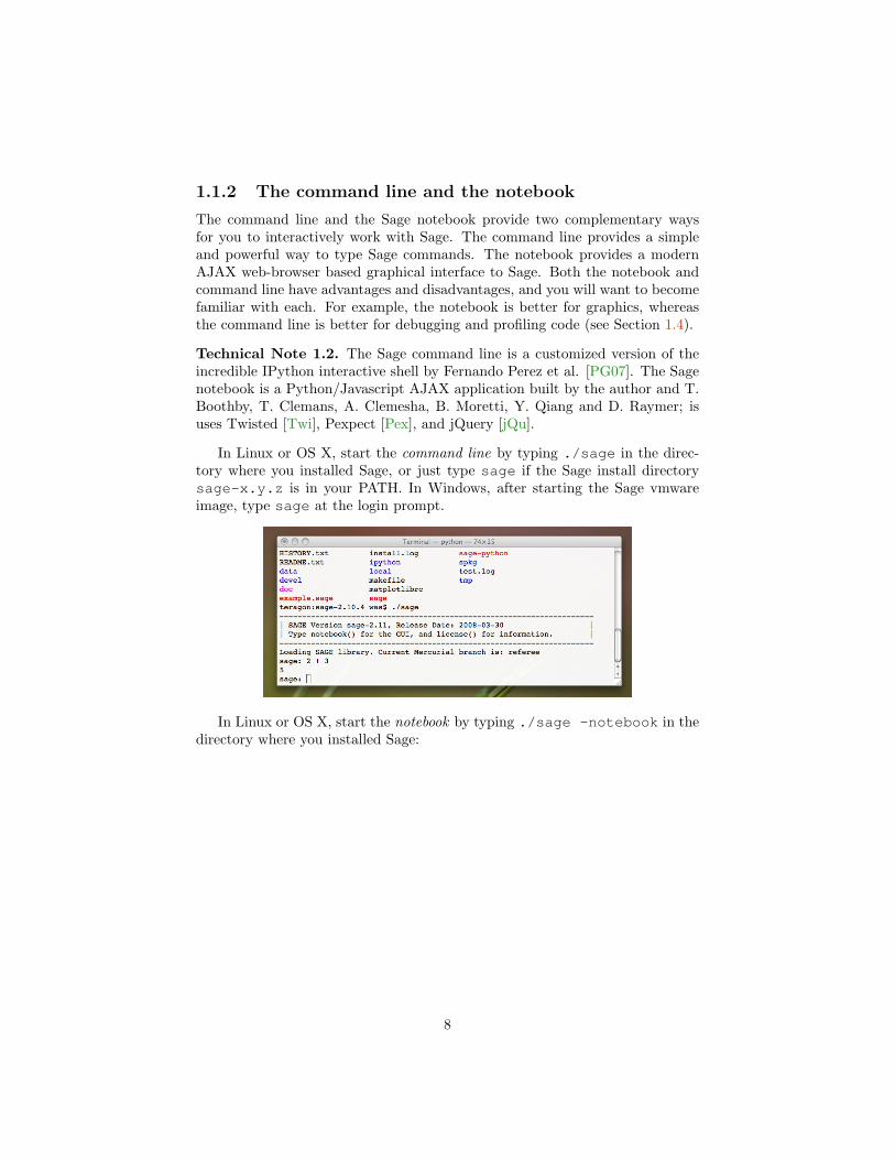
teragon:sage-2.10.4 was$ ./sage -inotebook----------------------------------------------------------------------| SAGE Version 2.10.4, Release Date: 2008-03-16 || Type notebook() for the GUI, and license() for information. |----------------------------------------------------------------------

Please wait while the SAGE Notebook server starts......The notebook files are stored in: /Users/was/.sage//sage_notebookWARNING: Running the notebook insecurely may be dangerous.Make sure you know what you are doing.

*************************************************** ** Open your web browser to http://localhost:8000 ** ***************************************************

In Windows, type notebook at the login prompt, then use your web browser tonavigate to the URL that is displayed. You can also use Sage without installingit on your computer by signing up for an account at https://sagenb.org.

Exercise 1.3.1. Using the Sage command line, compute 123 + 456.

2. Using the Sage notebook, compute 456 + 789.

Tab completion and help are incredibly useful features of both the commandline and notebook, and work in almost the same way in both. This is useful in

9

two ways. First, if you type the first few letters of a command, then press thetab key, you’ll see all commands that begin with those first few letters.

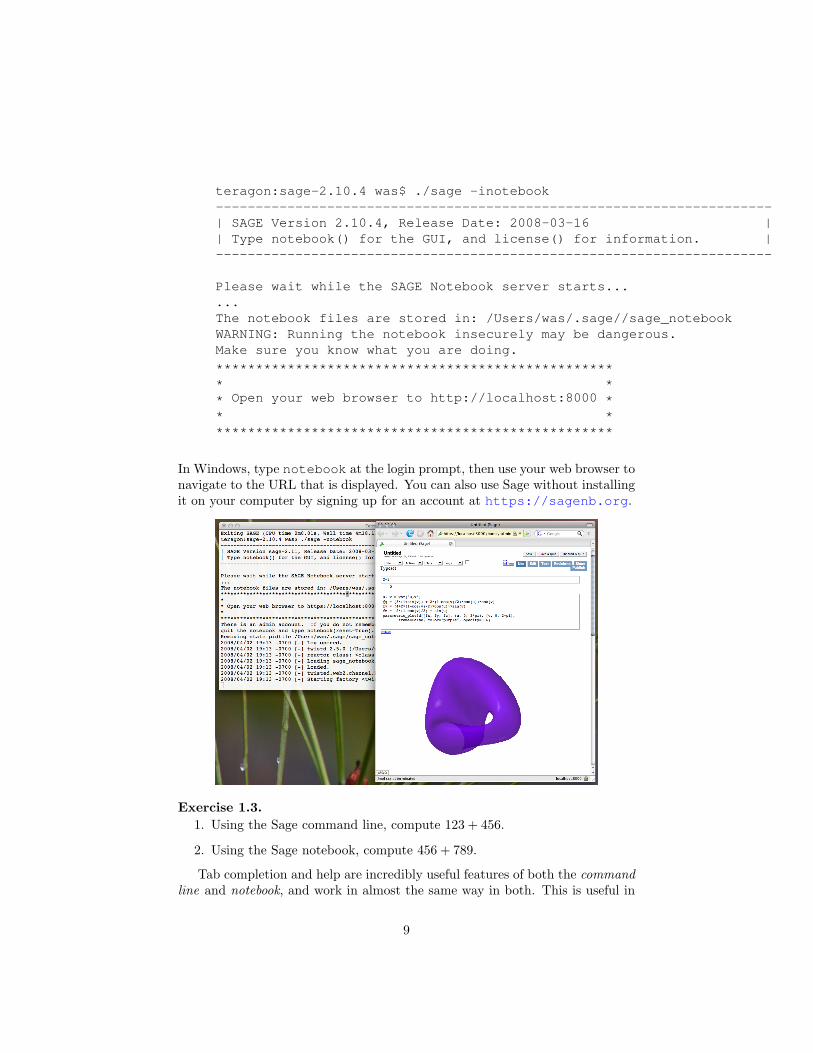
The second way in which tab completion is useful is that it shows you mostof the things you can do with something. For example, if n is an integer andyou type n.[tab key], you’ll see a list of all the functions that you can callon n. For example, the code n=2008 in Sage sets the variable n equal to theinteger 2008:

sage: n = 2008

Then type n.fa[tab key] (press the tab key after typing n.fa), you’ll seethat n.factor is a command associated to n. Type n.factor() to factor n:

sage: n = 2008sage: n.factor()2ˆ3 * 251

Here we are showing all input and output as if they were typed at thecommand line. If you’re using the notebook press shift-enter after typing n =2008 into an input cell. After computing the factorization you will see somethinglike this:

Exercise 1.4. Use tab completion to determine how to compute the factorialof 100.

In the command line every command you type is recorded in the history.Use the up arrow to scroll through previous commands; this history even worksif you quit Sage and restart. Likewise, in the notebook previous commands arevisibly recorded in input cells, and you can click or use the arrow keys to moveto a previous cell and press shift-enter to evaluate it again.

Exercise 1.5. 1. Quit the Sage command line, restart Sage, and press theup arrow until you see n = 2008. Change 2008 to 2009 and press enter.Then factor the result, again using the up arrow to select n.factor().

2. In the Sage notebook click and change n = 2008 to n = 2009, thenpress shift-enter twice to see how 2009 factors.

10

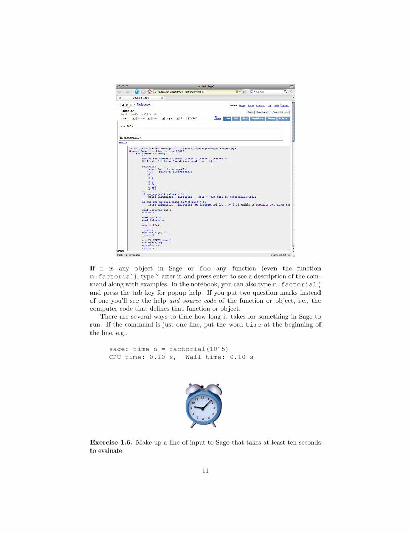
If n is any object in Sage or foo any function (even the functionn.factorial), type ? after it and press enter to see a description of the com-mand along with examples. In the notebook, you can also type n.factorial(and press the tab key for popup help. If you put two question marks insteadof one you’ll see the help and source code of the function or object, i.e., thecomputer code that defines that function or object.

There are several ways to time how long it takes for something in Sage torun. If the command is just one line, put the word time at the beginning ofthe line, e.g.,

sage: time n = factorial(10ˆ5)CPU time: 0.10 s, Wall time: 0.10 s

Exercise 1.6. Make up a line of input to Sage that takes at least ten secondsto evaluate.

11

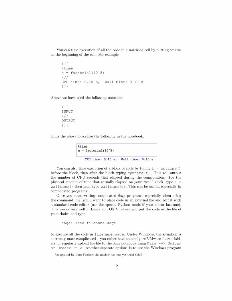
You can time execution of all the code in a notebook cell by putting %timeat the beginning of the cell. For example:

{{{%timen = factorial(10ˆ5)///CPU time: 0.10 s, Wall time: 0.10 s}}}

Above we have used the following notation:

{{{INPUT///OUTPUT}}}

Thus the above looks like the following in the notebook:

You can also time execution of a block of code by typing t = cputime()before the block, then after the block typing cputime(t). This will outputthe number of CPU seconds that elapsed during the computation. For thephysical amount of time that actually elapsed on your “wall” clock, type t =walltime() then later type walltime(t). This can be useful, especially incomplicated programs.

Once you start writing complicated Sage programs, especially when usingthe command line, you’ll want to place code in an external file and edit it witha standard code editor (use the special Python mode if your editor has one).This works very well in Linux and OS X, where you put the code in the file ofyour choice and type

sage: load filename.sage

to execute all the code in filename.sage. Under Windows, the situation iscurrently more complicated – you either have to configure VMware shared fold-ers, or regularly upload the file to the Sage notebook using Data --> Uploador Create File. Another separate option1 is to use the Windows program

1suggested by Lars Fischer; the author has not yet tried this!!

12

WinSCP [?]. Using WinSCP you can login to the VMware machine (use loginname ’login’ and password ’sage’). Then you can select edit from the contextmenu and edit files. WinSCP takes care of automatically uploading and down-loading the modified version of the file whenever you change it. If you call thefile filename.sage, you would type the following to load the file you’re editing:

sage: load /home/login/filename.sage

For OS X or Linux users, if you’re constantly editing filename.sage, andfind yourself regularly typing load filename.sage into Sage, you shouldinstead attach filename.sage by typing

sage: attach filename.sage

This works exactly like load filename.sage, except that iffilename.sage is changed and you execute a new command, Sagereloads filename.sage before executing the command. Try it; you’ll like it.

Exercise 1.7. Create a file hi.sage that contains the line print "hello".Load that file into Sage using the load command, and see that hello is printedout. If you’re using OS X or Linux, attach hi.sage, then change “hello”to something else, then type something at the Sage prompt – you should seesomething besides hello printed out.

1.1.3 Loading and saving variables and sessions

As mentioned above, in Sage you create a new variable by assigning to it. Forexample, typing n = 2008 creates a new variable n and assigns the value 2008to it. Most (but not all!2) individual variables, even incredibly complicatedones, can be easily saved or loaded to disk using the save and load functions.This can be extremely useful if it takes a long time to compute a variable, andyou want to save it to use it again later.

First we discuss using save and load from the command line, then from thenotebook. In the following command-line session, we set n to 2008, then save nto the variable myvar.sobj, quit sage, restart, and reload the value of n fromthat file.

2See the Python documentation on the pickle module.

13

teragon:˜ was$ sagesage: n = 2008sage: save(n, ’myvar’)sage: quitExiting SAGE (CPU time 0m0.02s, Wall time 0m41.28s).teragon:˜ was$ ls -l myvar.sobj-rw-r--r-- 1 was was 48 Mar 26 22:40 myvar.sobjteragon:˜ was$ sagesage: load(’myvar.sobj’)2008

Note that .sobj is added to the end of the filename, if it isn’t given. Also, allsaved objects are compressed to save disk space.

Using save and load from the notebook is a bit different, since every notebookcell is executed in a different subdirectory. In the following example, in the firstcell the value of n is saved in the file myvar.sobj in the current cell directory.In general, in the notebook every file created in the current (cell) directory iseither displayed embedded in the output or a link to it is created – you couldright click and download myvar.sobj to your hard drive if you wanted. In thesecond example we save the value of n to the file myvar.sobj in the directoryabove the current cell directory. This directory is fixed independent of the cellwe’re working in, so we can load myvar.sobj in another cell, which we do.

Not only can you load and save individual objects, but you can save allsave-able objects defined in the current session.3 In this example we define twovariables n = 2008 and m = −2/3, save the session, then restart, load thesession and see that n and m are again defined.

3WARNING: As of March 30, 2008, save session in the Sage notebook is broken.

14

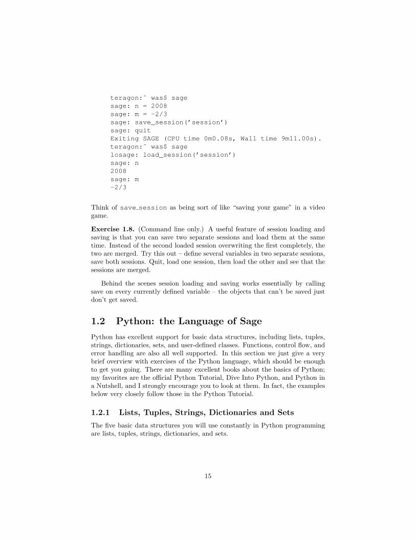
teragon:˜ was$ sagesage: n = 2008sage: m = -2/3sage: save_session(’session’)sage: quitExiting SAGE (CPU time 0m0.08s, Wall time 9m11.00s).teragon:˜ was$ sagelosage: load_session(’session’)sage: n2008sage: m-2/3

Think of save session as being sort of like “saving your game” in a videogame.

Exercise 1.8. (Command line only.) A useful feature of session loading andsaving is that you can save two separate sessions and load them at the sametime. Instead of the second loaded session overwriting the first completely, thetwo are merged. Try this out – define several variables in two separate sessions,save both sessions. Quit, load one session, then load the other and see that thesessions are merged.

Behind the scenes session loading and saving works essentially by callingsave on every currently defined variable – the objects that can’t be saved justdon’t get saved.

1.2 Python: the Language of Sage

Python has excellent support for basic data structures, including lists, tuples,strings, dictionaries, sets, and user-defined classes. Functions, control flow, anderror handling are also all well supported. In this section we just give a verybrief overview with exercises of the Python language, which should be enoughto get you going. There are many excellent books about the basics of Python;my favorites are the official Python Tutorial, Dive Into Python, and Python ina Nutshell, and I strongly encourage you to look at them. In fact, the examplesbelow very closely follow those in the Python Tutorial.

1.2.1 Lists, Tuples, Strings, Dictionaries and Sets

The five basic data structures you will use constantly in Python programmingare lists, tuples, strings, dictionaries, and sets.

15

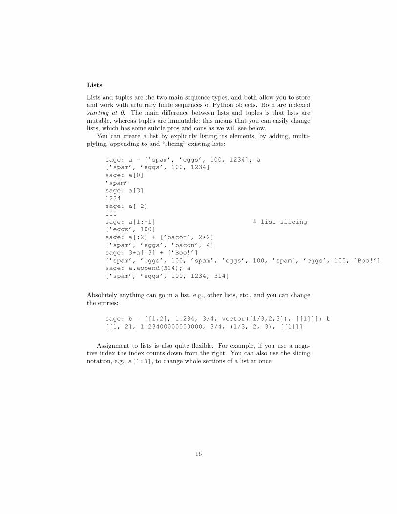
Lists

Lists and tuples are the two main sequence types, and both allow you to storeand work with arbitrary finite sequences of Python objects. Both are indexedstarting at 0. The main difference between lists and tuples is that lists aremutable, whereas tuples are immutable; this means that you can easily changelists, which has some subtle pros and cons as we will see below.

You can create a list by explicitly listing its elements, by adding, multi-plyling, appending to and “slicing” existing lists:

sage: a = [’spam’, ’eggs’, 100, 1234]; a[’spam’, ’eggs’, 100, 1234]sage: a[0]’spam’sage: a[3]1234sage: a[-2]100sage: a[1:-1] # list slicing[’eggs’, 100]sage: a[:2] + [’bacon’, 2*2][’spam’, ’eggs’, ’bacon’, 4]sage: 3*a[:3] + [’Boo!’][’spam’, ’eggs’, 100, ’spam’, ’eggs’, 100, ’spam’, ’eggs’, 100, ’Boo!’]sage: a.append(314); a[’spam’, ’eggs’, 100, 1234, 314]

Absolutely anything can go in a list, e.g., other lists, etc., and you can changethe entries:

sage: b = [[1,2], 1.234, 3/4, vector([1/3,2,3]), [[1]]]; b[[1, 2], 1.23400000000000, 3/4, (1/3, 2, 3), [[1]]]

Assignment to lists is also quite flexible. For example, if you use a nega-tive index the index counts down from the right. You can also use the slicingnotation, e.g., a[1:3], to change whole sections of a list at once.

16

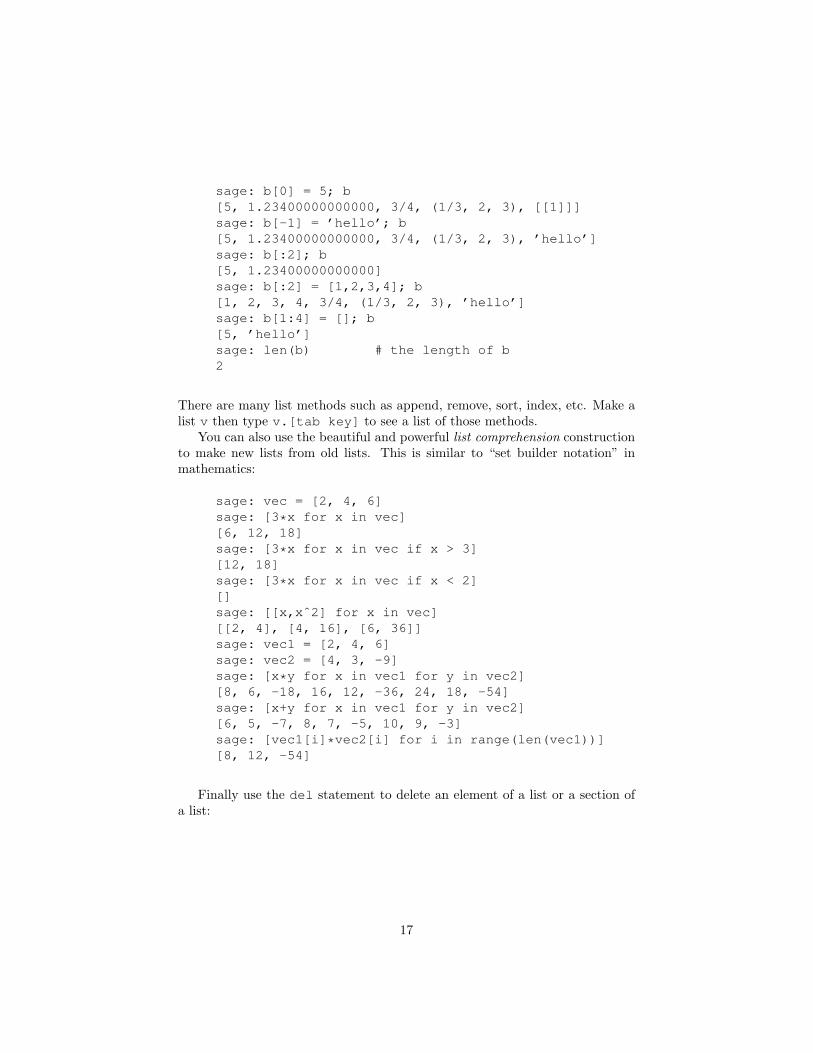
sage: b[0] = 5; b[5, 1.23400000000000, 3/4, (1/3, 2, 3), [[1]]]sage: b[-1] = ’hello’; b[5, 1.23400000000000, 3/4, (1/3, 2, 3), ’hello’]sage: b[:2]; b[5, 1.23400000000000]sage: b[:2] = [1,2,3,4]; b[1, 2, 3, 4, 3/4, (1/3, 2, 3), ’hello’]sage: b[1:4] = []; b[5, ’hello’]sage: len(b) # the length of b2

There are many list methods such as append, remove, sort, index, etc. Make alist v then type v.[tab key] to see a list of those methods.

You can also use the beautiful and powerful list comprehension constructionto make new lists from old lists. This is similar to “set builder notation” inmathematics:

sage: vec = [2, 4, 6]sage: [3*x for x in vec][6, 12, 18]sage: [3*x for x in vec if x > 3][12, 18]sage: [3*x for x in vec if x < 2][]sage: [[x,xˆ2] for x in vec][[2, 4], [4, 16], [6, 36]]sage: vec1 = [2, 4, 6]sage: vec2 = [4, 3, -9]sage: [x*y for x in vec1 for y in vec2][8, 6, -18, 16, 12, -36, 24, 18, -54]sage: [x+y for x in vec1 for y in vec2][6, 5, -7, 8, 7, -5, 10, 9, -3]sage: [vec1[i]*vec2[i] for i in range(len(vec1))][8, 12, -54]

Finally use the del statement to delete an element of a list or a section ofa list:

17

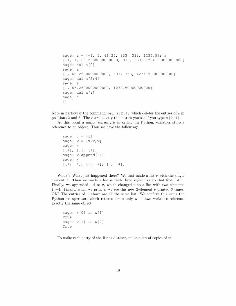
sage: a = [-1, 1, 66.25, 333, 333, 1234.5]; a[-1, 1, 66.2500000000000, 333, 333, 1234.50000000000]sage: del a[0]sage: a[1, 66.2500000000000, 333, 333, 1234.50000000000]sage: del a[2:4]sage: a[1, 66.2500000000000, 1234.50000000000]sage: del a[:]sage: a[]

Note in particular the command del a[2:4] which deletes the entries of a inpositions 2 and 3. These are exactly the entries you see if you type a[2:4].

At this point a major warning is in order. In Python, variables store areference to an object. Thus we have the following:

sage: v = [1]sage: w = [v,v,v]sage: w[[1], [1], [1]]sage: v.append(-4)sage: w[[1, -4], [1, -4], [1, -4]]

Whoa!? What just happened there? We first made a list v with the singleelement 1. Then we made a list w with three references to that first list v.Finally, we appended −4 to v, which changed v to a list with two elements1,−4. Finally, when we print w we see this new 2-element v printed 3 times.OK? The entries of w above are all the same list. We confirm this using thePython is operator, which returns True only when two variables referenceexactly the same object:

sage: w[0] is w[1]Truesage: w[1] is w[2]True

To make each entry of the list w distinct, make a list of copies of v:

18

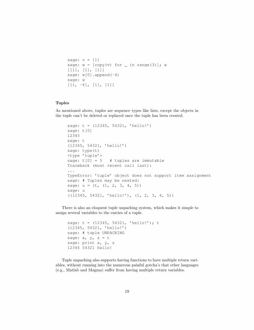
sage: v = [1]sage: w = [copy(v) for _ in range(3)]; w[[1], [1], [1]]sage: w[0].append(-4)sage: w[[1, -4], [1], [1]]

Tuples

As mentioned above, tuples are sequence types like lists, except the objects inthe tuple can’t be deleted or replaced once the tuple has been created.

sage: t = (12345, 54321, ’hello!’)sage: t[0]12345sage: t(12345, 54321, ’hello!’)sage: type(t)<type ’tuple’>sage: t[0] = 5 # tuples are immutableTraceback (most recent call last):...TypeError: ’tuple’ object does not support item assignmentsage: # Tuples may be nested:sage: u = (t, (1, 2, 3, 4, 5))sage: u((12345, 54321, ’hello!’), (1, 2, 3, 4, 5))

There is also an eloquent tuple unpacking system, which makes it simple toassign several variables to the entries of a tuple.

sage: t = (12345, 54321, ’hello!’); t(12345, 54321, ’hello!’)sage: # tuple UNPACKINGsage: x, y, z = tsage: print x, y, z12345 54321 hello!

Tuple unpacking also supports having functions to have multiple return vari-ables, without running into the numerous painful gotcha’s that other languages(e.g., Matlab and Magma) suffer from having multiple return variables.

19

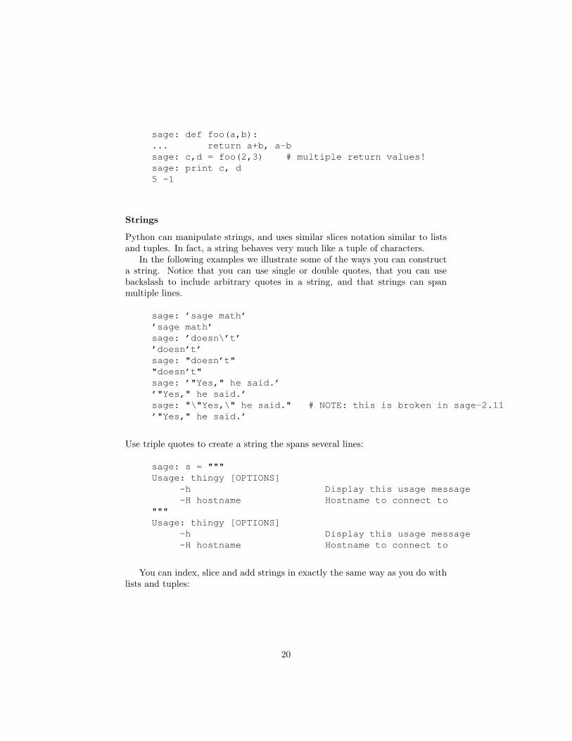
sage: def foo(a,b):... return a+b, a-bsage: c,d = foo(2,3) # multiple return values!sage: print c, d5 -1

Strings

Python can manipulate strings, and uses similar slices notation similar to listsand tuples. In fact, a string behaves very much like a tuple of characters.

In the following examples we illustrate some of the ways you can constructa string. Notice that you can use single or double quotes, that you can usebackslash to include arbitrary quotes in a string, and that strings can spanmultiple lines.

sage: ’sage math’’sage math’sage: ’doesn\’t’’doesn’t’sage: "doesn’t""doesn’t"sage: ’"Yes," he said.’’"Yes," he said.’sage: "\"Yes,\" he said." # NOTE: this is broken in sage-2.11’"Yes," he said.’

Use triple quotes to create a string the spans several lines:

sage: s = """Usage: thingy [OPTIONS]

-h Display this usage message-H hostname Hostname to connect to

"""Usage: thingy [OPTIONS]

-h Display this usage message-H hostname Hostname to connect to

You can index, slice and add strings in exactly the same way as you do withlists and tuples:

20

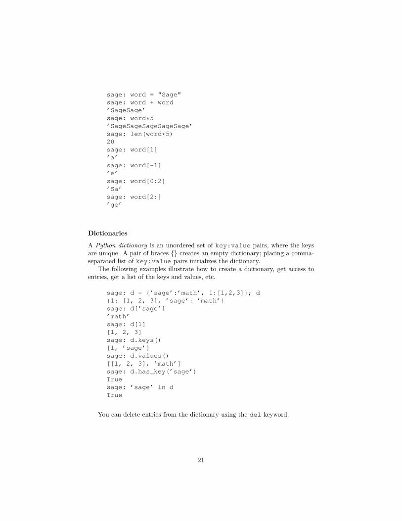
sage: word = "Sage"sage: word + word’SageSage’sage: word*5’SageSageSageSageSage’sage: len(word*5)20sage: word[1]’a’sage: word[-1]’e’sage: word[0:2]’Sa’sage: word[2:]’ge’

Dictionaries

A Python dictionary is an unordered set of key:value pairs, where the keysare unique. A pair of braces {} creates an empty dictionary; placing a comma-separated list of key:value pairs initializes the dictionary.

The following examples illustrate how to create a dictionary, get access toentries, get a list of the keys and values, etc.

sage: d = {’sage’:’math’, 1:[1,2,3]}; d{1: [1, 2, 3], ’sage’: ’math’}sage: d[’sage’]’math’sage: d[1][1, 2, 3]sage: d.keys()[1, ’sage’]sage: d.values()[[1, 2, 3], ’math’]sage: d.has_key(’sage’)Truesage: ’sage’ in dTrue

You can delete entries from the dictionary using the del keyword.

21

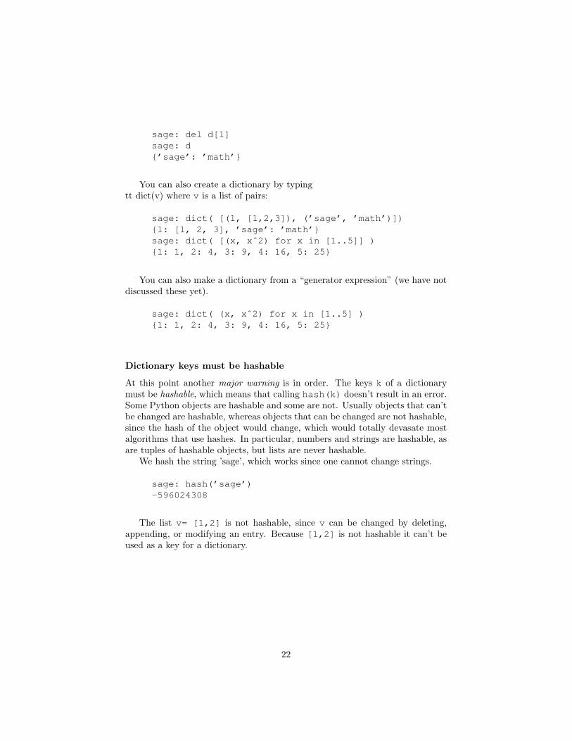
sage: del d[1]sage: d{’sage’: ’math’}

You can also create a dictionary by typingtt dict(v) where v is a list of pairs:

sage: dict( [(1, [1,2,3]), (’sage’, ’math’)]){1: [1, 2, 3], ’sage’: ’math’}sage: dict( [(x, xˆ2) for x in [1..5]] ){1: 1, 2: 4, 3: 9, 4: 16, 5: 25}

You can also make a dictionary from a “generator expression” (we have notdiscussed these yet).

sage: dict( (x, xˆ2) for x in [1..5] ){1: 1, 2: 4, 3: 9, 4: 16, 5: 25}

Dictionary keys must be hashable

At this point another major warning is in order. The keys k of a dictionarymust be hashable, which means that calling hash(k) doesn’t result in an error.Some Python objects are hashable and some are not. Usually objects that can’tbe changed are hashable, whereas objects that can be changed are not hashable,since the hash of the object would change, which would totally devasate mostalgorithms that use hashes. In particular, numbers and strings are hashable, asare tuples of hashable objects, but lists are never hashable.

We hash the string ’sage’, which works since one cannot change strings.

sage: hash(’sage’)-596024308

The list v= [1,2] is not hashable, since v can be changed by deleting,appending, or modifying an entry. Because [1,2] is not hashable it can’t beused as a key for a dictionary.

22

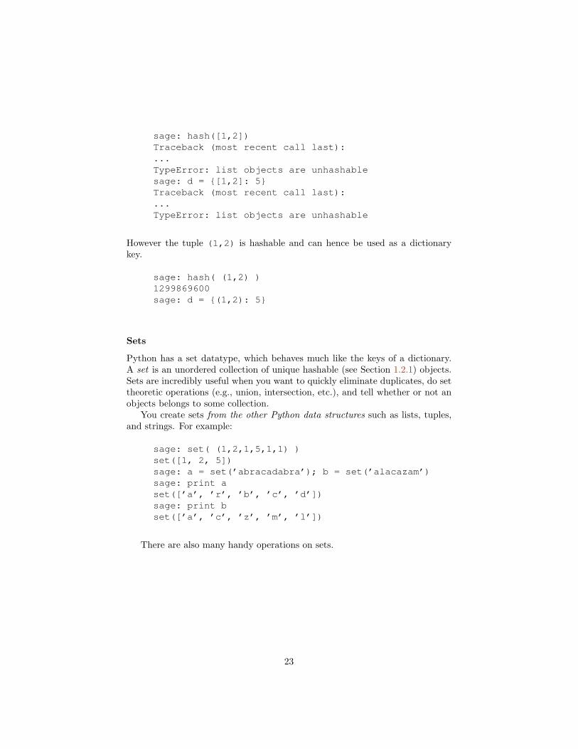
sage: hash([1,2])Traceback (most recent call last):...TypeError: list objects are unhashablesage: d = {[1,2]: 5}Traceback (most recent call last):...TypeError: list objects are unhashable

However the tuple (1,2) is hashable and can hence be used as a dictionarykey.

sage: hash( (1,2) )1299869600sage: d = {(1,2): 5}

Sets

Python has a set datatype, which behaves much like the keys of a dictionary.A set is an unordered collection of unique hashable (see Section 1.2.1) objects.Sets are incredibly useful when you want to quickly eliminate duplicates, do settheoretic operations (e.g., union, intersection, etc.), and tell whether or not anobjects belongs to some collection.

You create sets from the other Python data structures such as lists, tuples,and strings. For example:

sage: set( (1,2,1,5,1,1) )set([1, 2, 5])sage: a = set(’abracadabra’); b = set(’alacazam’)sage: print aset([’a’, ’r’, ’b’, ’c’, ’d’])sage: print bset([’a’, ’c’, ’z’, ’m’, ’l’])

There are also many handy operations on sets.

23

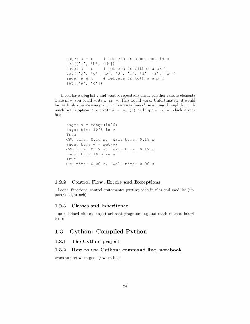
sage: a - b # letters in a but not in bset([’r’, ’b’, ’d’])sage: a | b # letters in either a or bset([’a’, ’c’, ’b’, ’d’, ’m’, ’l’, ’r’, ’z’])sage: a & b # letters in both a and bset([’a’, ’c’])

If you have a big list v and want to repeatedly check whether various elementsx are in v, you could write x in v. This would work. Unfortunately, it wouldbe really slow, since every x in v requires linearly searching through for x. Amuch better option is to create w = set(v) and type x in w, which is veryfast.

sage: v = range(10ˆ6)sage: time 10ˆ5 in vTrueCPU time: 0.16 s, Wall time: 0.18 ssage: time w = set(v)CPU time: 0.12 s, Wall time: 0.12 ssage: time 10ˆ5 in wTrueCPU time: 0.00 s, Wall time: 0.00 s

1.2.2 Control Flow, Errors and Exceptions

- Loops, functions, control statements; putting code in files and modules (im-port/load/attach)

1.2.3 Classes and Inheritence

- user-defined classes; object-oriented programming and mathematics, inheri-tence

1.3 Cython: Compiled Python

1.3.1 The Cython project

1.3.2 How to use Cython: command line, notebook

when to use; when good / when bad

24

1.4 Debugging and Profiling

The best perspective to take when writing or indeed using code is to assumethat it has bugs. Be skeptical! If you read source code of Sage or its componentsyou’ll sometimes see things that will make you worry. This is a good thing, e.g.,this occurs in a comment in the Sage code by Jonathan Bober for computing thenumber of partitions of an integer (the number of partitions command):

// Extensive trial and error has found 3 to be the smallest// value that doesn’t seem to produce any wrong answers.// Thus, to be safe, we use 5 extra bits.

Note, by the way, that Bober’s code for computing the number of partitionsof an integer is currently faster than anything else in the world, and it is notknown to have any bugs.

A healthy amount of skepticism and worry is a good to cultivate when doingcomputational mathematics. Never listen to anybody who suggests you dootherwise. These same sort of issues occur in closed source systems such asMathematica, but you don’t get to see them – that doesn’t make the chance ofbugs less likely. In fact, the Mathematica documentation says the following:

But just as long proofs will inevitably contain errors that go un-detected for many years, so also a complex software system suchas Mathematica will contain errors that go undetected even aftermillions of people have used it.

There can even be bugs in the implementation of basic arithmetic, even at thehardware level! [[reference the pentium hardware bug from the 1990s that wasfound by a number theorist trying to debug his code]] So be skeptical when youdo computations. Always think about what mathematical computations tellyou, and try to find ways to double check results.

It almost goes without saying, but beautifully written, well-documented codethat has been around for a long time and used a great deal is generally muchless likely to be seriously buggy than newly written code. A great example ofsuch high quality – by aging – code is NTL (the Number Theory Library [[url]]).Quality code that has been used for years, and thus likely has few bugs is likegold – treat it that way; don’t just toss it out and assume that something newthat you sit down and write is likely to be better. That said, if you persist youcan and will write beautiful code that equals or surpasses anything ever donebefore. When you do this, please consider contributing you code to the Sageproject.

There are several good reasons to write new code. One excellent reason isthat you simply want to understand an algorithm well, perhaps one you’re learn-ing about in a course, a book, a paper, or that you just designed. Implementingan algorithm correctly forces you to understand every detail, which can providenew insight into the algorithm. If you’re implementing a nontrivial algorithm

25

that is described in a book or paper, the chances that it is wrong in some way(e.g., a typo in a formula, a fundamental mistake in the algorithm, whatever)is quite high – so you will definitely learn something, and possibly improve themathematical literature while you’re at it.

Another great reason to write new code is to implement an algorithm thatisn’t available in Sage. When you do this, make sure to be skeptical about thecorrectness of your code; always test it extensively, document it, etc., just toincrease the chances it might always work correctly. And if there is any wayto independently verify correctness of the output of code, attempt to imple-ment this too. If the algorithm is available in other mathematical software suchas Maple or Mathematica, and you have that program, use the interfaces de-scribed in Section 1.6 to write code that automatically tests the output of yourimplementation against the output of the implementation in that other system.Include such test code in your final product.

1.4.1 Using Print Statements

Yes, you can use print statements for debugging your code. There is no shamein this! Especially when using Python where you do not have to recompile everytime, this can be a particularly useful technique.

specific techniques for using print statements (how to figure out things)use attach for .py or .sage files.

1.4.2 Debugging Python using pdb

Use command line and do %pdb

1.4.3 Debugging Cython using gdb

how to trace things throughbt is enough to get pretty farmultiple processes can be confusing

1.5 Source Control Management

1.5.1 Distributed versus Centralized

1.5.2 Mercurial

1.6 Using Mathematica, Matlab, Maple, etc.,from Sage

A distinctive feature of Sage is that Sage supports using Maple, Mathematica,Octave, Matlab, and many other programs from Sage, assuming you have the

26

relevant program (there are some caveats). This makes it much easier to combinethe functionality of these systems with each other and Sage.

Before discussing interfaces in more detail, we make a few operating systemdependent remarks.

what works on all os’s; in particular gap, singular, gp, maxima, always there.what works on linuxon os xon windows—-example of using gp to do something.example of using mathematicaexample of using mapleexample of using matlab/octave—-eval versus call.Discussion of what goes on behind the scenes. Files used for large inputs –

named pipes for small.—-Warning– multiple processes; complicated; can get parallel, which is harder

to think about...

27

Chapter 2

Algebraic Computing

Algebraic computing is concerned with computing with the algebraic objects ofmathematics such as arbitrary precision integer and rational numbers, groups,rings, fields, vector spaces and matrices, and other object. The tools of algebraiccomputing support research and education in pure mathematics, underly thedesign of error correcting codes and cryptographical systems, and play a role inscientific and statistical computing.

2.1 Groups, Rings and Fields

2.1.1 Groups

2.1.2 Rings

2.1.3 Fields

2.2 Number Theory

2.2.1 Prime numbers and integer factorization

2.2.2 Elliptic curves

2.2.3 Public-key cryptography: Diffie-Hellman, RSA, andElliptic curve

2.3 Linear Algebra

2.3.1 Matrix arithmetic and echelon form

Matrix multiplication using a numerical BLAS (in both mod p and over ZZcases)

28

2.3.2 Vector spaces and free modules

2.3.3 Solving linear systems

Applicatin: computing determinants over ZZ

2.4 Systems of polynomial equations

2.5 Graph Theory

2.5.1 Creating graphs and plotting them

2.5.2 Computing automorphisms and isomorphisms

2.5.3 The genus and other invariants

29

Chapter 3

Scientific Computing

Scientific computing is concerned with constructing mathematical models andusing numerical techniques to solve scientific, social, and engineering problems.

30

3.1 Floating Point Numbers

3.1.1 Machine precision floating point numbers

3.1.2 Arbitrary precision floating point numbers

3.2 Interval arithmetic

3.3 Root Finding and Optimization

3.3.1 Single variable: max, min, roots, rational root iso-lation

3.3.2 Multivariable: local max, min, roots

3.4 NumericalSolution of Linear Systems

3.4.1 Solving linear systems using LU factorization

3.4.2 Solving linear systems iteratively

3.4.3 Eigenvalues and eigenvectors

3.5 Symbolic Calculus

3.5.1 Symbolic Differentiation and integration

3.5.2 Symbolic Limits and Taylor series

3.5.3 Numerical Integration

31

Chapter 4

Statistical Computing

4.1 Introduction to R and Scipy.stats

4.1.1 The R System for Statistical Computing

4.1.2 The Scipy.stats Python Library

4.2 Descriptive Statistics

4.2.1 Mean, standard deviation, etc.

4.3 Inferential Statistics

4.3.1 Simple Inference

4.3.2 Conditional Inference

4.4 Regression

4.4.1 Linear regression

4.4.2 Logistic regression

32

Bibliography

[ABC+] B. Allombert, K. Belabas, H. Cohen, X. Roblot, and I. Zakharevitch,PARI/GP, http://pari.math.u-bordeaux.fr/.

[BCP97] W. Bosma, J. Cannon, and C. Playoust, The Magma algebra system.I. The user language, J. Symbolic Comput. 24 (1997), no. 3–4, 235–265, Computational algebra and number theory (London, 1993). MR1 484 478

[jQu] jQuery, A new type of javascript library, http://www.4dsolutions.net/ocn/overcome.html.

[Pex] Pexpect, A pure python expect-like module, http://www.noah.org/wiki/Pexpect#Download and Installation.

[PG07] Fernando. Perez and Brian E. Granger, IPython: a System for Inter-active Scientific Computing, Comput. Sci. Eng. 9 (2007), no. 3, 21–29,University of Colorado APPM Preprint #549.

[Twi] Twisted, A framework for networked applications, http://twistedmatrix.com.

33