Embed Size (px)
Citation preview
OutlineIntroduction
Basic existence theoryRegularity
End of first part
An introduction to Hamilton-Jacobi equations
Stefano Bianchini
February 2, 2011
Stefano Bianchini An introduction to Hamilton-Jacobi equations

OutlineIntroduction
Basic existence theoryRegularity
End of first part
IntroductionHamilton’s principal functionClassical limit of SchrodingerA study case in calculus of variationsControl theoryOptimal mass transportation
Basic existence theoryExistence in the Lipschitz classViscosity solutionsLagrangian formulation
RegularitySome simple computationsA regularity resultRegularity for hyperbolic conservation laws
End of first partOutline of the second partBibliography
Stefano Bianchini An introduction to Hamilton-Jacobi equations
OutlineIntroduction
Basic existence theoryRegularity
End of first part
Hamilton’s principal functionClassical limit of SchrodingerA study case in calculus of variationsControl theoryOptimal mass transportation
Outline
IntroductionHamilton’s principal functionClassical limit of SchrodingerA study case in calculus of variationsControl theoryOptimal mass transportation
Basic existence theory
Regularity
End of first part
Stefano Bianchini An introduction to Hamilton-Jacobi equations
OutlineIntroduction
Basic existence theoryRegularity
End of first part
Hamilton’s principal functionClassical limit of SchrodingerA study case in calculus of variationsControl theoryOptimal mass transportation
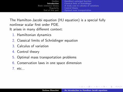
The Hamilton-Jacobi equation (HJ equation) is a special fullynonlinear scalar first order PDE.It arises in many different context:
1. Hamiltonian dynamics
2. Classical limits of Schrodinger equation
3. Calculus of variation
4. Control theory
5. Optimal mass transportation problems
6. Conservation laws in one space dimension
7. etc...
Even if it is fully nonlinear, there is a satisfactory theory ofexistence and regularity of solutions.
Stefano Bianchini An introduction to Hamilton-Jacobi equations

OutlineIntroduction
Basic existence theoryRegularity
End of first part
Hamilton’s principal functionClassical limit of SchrodingerA study case in calculus of variationsControl theoryOptimal mass transportation
The Hamilton-Jacobi equation (HJ equation) is a special fullynonlinear scalar first order PDE.It arises in many different context:
1. Hamiltonian dynamics
2. Classical limits of Schrodinger equation
3. Calculus of variation
4. Control theory
5. Optimal mass transportation problems
6. Conservation laws in one space dimension
7. etc...
Even if it is fully nonlinear, there is a satisfactory theory ofexistence and regularity of solutions.
Stefano Bianchini An introduction to Hamilton-Jacobi equations
OutlineIntroduction
Basic existence theoryRegularity
End of first part
Hamilton’s principal functionClassical limit of SchrodingerA study case in calculus of variationsControl theoryOptimal mass transportation
Hamilton’s principal function
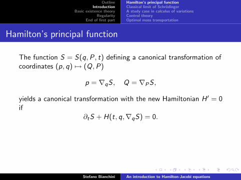
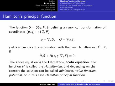
The function S = S(q,P, t) defining a canonical transformation ofcoordinates (p, q) 7→ (Q,P)
p = ∇qS , Q = ∇PS ,
yields a canonical transformation with the new Hamiltonian H ′ = 0if
∂tS + H(t, q,∇qS) = 0.
The above equation is the Hamilton-Jacobi equation: thefunction H is called the Hamiltonian, and depending on thecontext the solution can be called minimizer, value function,potential, or in this case Hamilton principal function.
Stefano Bianchini An introduction to Hamilton-Jacobi equations
OutlineIntroduction
Basic existence theoryRegularity
End of first part
Hamilton’s principal functionClassical limit of SchrodingerA study case in calculus of variationsControl theoryOptimal mass transportation
Hamilton’s principal function
The function S = S(q,P, t) defining a canonical transformation ofcoordinates (p, q) 7→ (Q,P)
p = ∇qS , Q = ∇PS ,
yields a canonical transformation with the new Hamiltonian H ′ = 0if
∂tS + H(t, q,∇qS) = 0.
The above equation is the Hamilton-Jacobi equation: thefunction H is called the Hamiltonian, and depending on thecontext the solution can be called minimizer, value function,potential, or in this case Hamilton principal function.
Stefano Bianchini An introduction to Hamilton-Jacobi equations
OutlineIntroduction
Basic existence theoryRegularity
End of first part
Hamilton’s principal functionClassical limit of SchrodingerA study case in calculus of variationsControl theoryOptimal mass transportation
Schrodinger equation
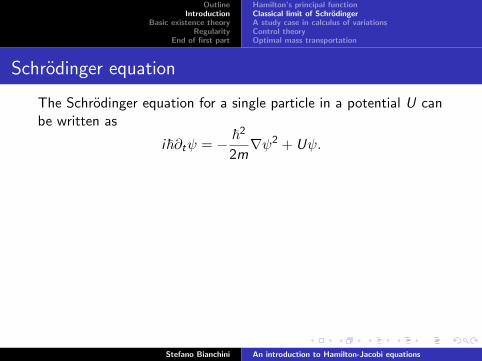
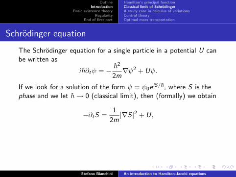
The Schrodinger equation for a single particle in a potential U canbe written as
i~∂tψ = − ~2
2m∇ψ2 + Uψ.
If we look for a solution of the form ψ = ψ0eiS/~, where S is the
phase and we let ~→ 0 (classical limit), then (formally) we obtain
−∂tS =1
2m|∇S |2 + U,
which is the Hamilton-Jacobi equation for the Hamiltonian
H =p2
2m+ U.
Stefano Bianchini An introduction to Hamilton-Jacobi equations
OutlineIntroduction
Basic existence theoryRegularity
End of first part
Hamilton’s principal functionClassical limit of SchrodingerA study case in calculus of variationsControl theoryOptimal mass transportation
Schrodinger equation
The Schrodinger equation for a single particle in a potential U canbe written as
i~∂tψ = − ~2
2m∇ψ2 + Uψ.
If we look for a solution of the form ψ = ψ0eiS/~, where S is the
phase and we let ~→ 0 (classical limit), then (formally) we obtain
−∂tS =1
2m|∇S |2 + U,
which is the Hamilton-Jacobi equation for the Hamiltonian
H =p2
2m+ U.
Stefano Bianchini An introduction to Hamilton-Jacobi equations
OutlineIntroduction
Basic existence theoryRegularity
End of first part
Hamilton’s principal functionClassical limit of SchrodingerA study case in calculus of variationsControl theoryOptimal mass transportation
Calculus of variation
Consider the minimization problem in Ω ⊂ Rd
min
∫ (1I|p|≤1(∇u(x)) + u(x)
)dx : u|∂Ω = u0
.
The solution satisfies the time independent Hamilton-Jacobiequation
1− |∇u| = 0,
with the Hamiltonian |p| and boundary data u0.The Euler-Lagrange equation reads as
div(ρd) = 1,
with d the direction of the optimal ray (see later).
Stefano Bianchini An introduction to Hamilton-Jacobi equations
OutlineIntroduction
Basic existence theoryRegularity
End of first part
Hamilton’s principal functionClassical limit of SchrodingerA study case in calculus of variationsControl theoryOptimal mass transportation
Calculus of variation
Consider the minimization problem in Ω ⊂ Rd
min
∫ (1I|p|≤1(∇u(x)) + u(x)
)dx : u|∂Ω = u0
.
The solution satisfies the time independent Hamilton-Jacobiequation
1− |∇u| = 0,
with the Hamiltonian |p| and boundary data u0.
The Euler-Lagrange equation reads as
div(ρd) = 1,
with d the direction of the optimal ray (see later).
Stefano Bianchini An introduction to Hamilton-Jacobi equations
OutlineIntroduction
Basic existence theoryRegularity
End of first part
Hamilton’s principal functionClassical limit of SchrodingerA study case in calculus of variationsControl theoryOptimal mass transportation
Calculus of variation
Consider the minimization problem in Ω ⊂ Rd
min
∫ (1I|p|≤1(∇u(x)) + u(x)
)dx : u|∂Ω = u0
.
The solution satisfies the time independent Hamilton-Jacobiequation
1− |∇u| = 0,
with the Hamiltonian |p| and boundary data u0.The Euler-Lagrange equation reads as
div(ρd) = 1,
with d the direction of the optimal ray (see later).
Stefano Bianchini An introduction to Hamilton-Jacobi equations
OutlineIntroduction
Basic existence theoryRegularity
End of first part
Hamilton’s principal functionClassical limit of SchrodingerA study case in calculus of variationsControl theoryOptimal mass transportation
Control theory
Consider the ODE
x = f (x , u), u control,
and the problem is to minimize the functional
A(t) = minu
∫ T
tL(x , u)dt + F (x(T ))
.
DefiningH(t, x , p) := min
u
p · f (x , u) + L(x , u)
,
the function A(t) satisfies the Hamilton-Jacobi-Bellman equation
∂tA + H(t, x ,∇A) = 0, A(T ) = F (x).
Stefano Bianchini An introduction to Hamilton-Jacobi equations
OutlineIntroduction
Basic existence theoryRegularity
End of first part
Hamilton’s principal functionClassical limit of SchrodingerA study case in calculus of variationsControl theoryOptimal mass transportation
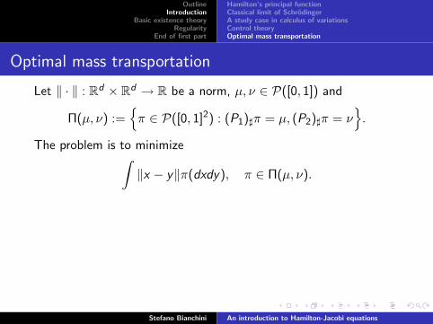
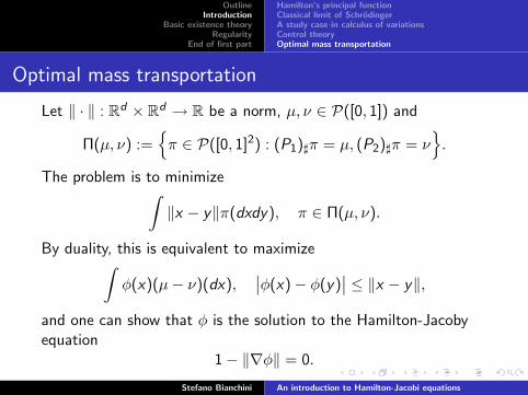
Optimal mass transportation
Let ‖ · ‖ : Rd × Rd → R be a norm, µ, ν ∈ P([0, 1]) and
Π(µ, ν) :=π ∈ P([0, 1]2) : (P1)]π = µ, (P2)]π = ν
.
The problem is to minimize∫‖x − y‖π(dxdy), π ∈ Π(µ, ν).
By duality, this is equivalent to maximize∫φ(x)(µ− ν)(dx),
∣∣φ(x)− φ(y)∣∣ ≤ ‖x − y‖,
and one can show that φ is the solution to the Hamilton-Jacobyequation
1− ‖∇φ‖ = 0.
Stefano Bianchini An introduction to Hamilton-Jacobi equations
OutlineIntroduction
Basic existence theoryRegularity
End of first part
Hamilton’s principal functionClassical limit of SchrodingerA study case in calculus of variationsControl theoryOptimal mass transportation
Optimal mass transportation
Let ‖ · ‖ : Rd × Rd → R be a norm, µ, ν ∈ P([0, 1]) and
Π(µ, ν) :=π ∈ P([0, 1]2) : (P1)]π = µ, (P2)]π = ν
.
The problem is to minimize∫‖x − y‖π(dxdy), π ∈ Π(µ, ν).
By duality, this is equivalent to maximize∫φ(x)(µ− ν)(dx),
∣∣φ(x)− φ(y)∣∣ ≤ ‖x − y‖,
and one can show that φ is the solution to the Hamilton-Jacobyequation
1− ‖∇φ‖ = 0.
Stefano Bianchini An introduction to Hamilton-Jacobi equations

OutlineIntroduction
Basic existence theoryRegularity
End of first part
Hamilton’s principal functionClassical limit of SchrodingerA study case in calculus of variationsControl theoryOptimal mass transportation
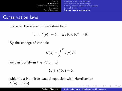
Conservation laws
Consider the scalar conservation laws
ut + f (u)x = 0, u : R× R+ → R.
By the change of variable
U(x) =
∫ x
u(y)dy ,
we can transform the PDE into
Ut + f (Ux) = 0,
which is a Hamilton-Jacobi equation with HamiltonianH(p) = f (p).
Stefano Bianchini An introduction to Hamilton-Jacobi equations
OutlineIntroduction
Basic existence theoryRegularity
End of first part
Hamilton’s principal functionClassical limit of SchrodingerA study case in calculus of variationsControl theoryOptimal mass transportation
Conservation laws
Consider the scalar conservation laws
ut + f (u)x = 0, u : R× R+ → R.
By the change of variable
U(x) =
∫ x
u(y)dy ,
we can transform the PDE into
Ut + f (Ux) = 0,
which is a Hamilton-Jacobi equation with HamiltonianH(p) = f (p).
Stefano Bianchini An introduction to Hamilton-Jacobi equations
OutlineIntroduction
Basic existence theoryRegularity
End of first part
Existence in the Lipschitz classViscosity solutionsLagrangian formulation
Outline
Introduction
Basic existence theoryExistence in the Lipschitz classViscosity solutionsLagrangian formulation
Regularity
End of first part
Stefano Bianchini An introduction to Hamilton-Jacobi equations
OutlineIntroduction
Basic existence theoryRegularity
End of first part
Existence in the Lipschitz classViscosity solutionsLagrangian formulation
What we can expect
The natural space of functions where the solutions lives isLipschitz.
Example. The model Hamiltonian is p2
2 , and the function
u(t, x) = −∫ x
0min
1,−y
t
dy
is a regular solution for t < 1 to
ut +|ux |2
2= 0.
At t = 1 the solution becomes only 1-Lipschitz.
Stefano Bianchini An introduction to Hamilton-Jacobi equations
OutlineIntroduction
Basic existence theoryRegularity
End of first part
Existence in the Lipschitz classViscosity solutionsLagrangian formulation
A solution to Hamilton-Jacobi can be defined as a Lipschitzfunction u : R+ × Rd → R such that
ut + H(t, x ,∇u) = 0
is satisfied at every differentiable point of u, i.e. Ld+1-a.e..
A solution in the above “a.e.-sense” is not unique.Example. The function
u(t, x) = min
|x | − t
2, 0
,
satisfies
ut +|ux |2
2= 0, u(0, x) = 0.
Clearly the expected solution is u(t, x) = 0.
Stefano Bianchini An introduction to Hamilton-Jacobi equations

OutlineIntroduction
Basic existence theoryRegularity
End of first part
Existence in the Lipschitz classViscosity solutionsLagrangian formulation
A solution to Hamilton-Jacobi can be defined as a Lipschitzfunction u : R+ × Rd → R such that
ut + H(t, x ,∇u) = 0
is satisfied at every differentiable point of u, i.e. Ld+1-a.e..A solution in the above “a.e.-sense” is not unique.
Example. The function
u(t, x) = min
|x | − t
2, 0
,
satisfies
ut +|ux |2
2= 0, u(0, x) = 0.
Clearly the expected solution is u(t, x) = 0.
Stefano Bianchini An introduction to Hamilton-Jacobi equations

OutlineIntroduction
Basic existence theoryRegularity
End of first part
Existence in the Lipschitz classViscosity solutionsLagrangian formulation
A solution to Hamilton-Jacobi can be defined as a Lipschitzfunction u : R+ × Rd → R such that
ut + H(t, x ,∇u) = 0
is satisfied at every differentiable point of u, i.e. Ld+1-a.e..A solution in the above “a.e.-sense” is not unique.Example. The function
u(t, x) = min
|x | − t
2, 0
,
satisfies
ut +|ux |2
2= 0, u(0, x) = 0.
Clearly the expected solution is u(t, x) = 0.
Stefano Bianchini An introduction to Hamilton-Jacobi equations

OutlineIntroduction
Basic existence theoryRegularity
End of first part
Existence in the Lipschitz classViscosity solutionsLagrangian formulation
Maximum principle
For scalar equation, a natural requirement is
u(0, x) ≤ v(0, x) ⇒ u(t, x) ≤ v(t, x).
We can restrict the possible solutions to the ones generating asemigroup satisfying the maximum principle.
If φ is a regular function such that uε − φ has a local minimum in(t, x), then it follows
∆(uε − φ) ≥ 0,
Since ∇uε = ∇φ, uεt = φt , we recover
φt + H(t, x ,∇φ)− ε∆φ ≥ 0,
and in the limitφt + H(t, x ,∇φ) ≥ 0.
Stefano Bianchini An introduction to Hamilton-Jacobi equations
OutlineIntroduction
Basic existence theoryRegularity
End of first part
Existence in the Lipschitz classViscosity solutionsLagrangian formulation
Maximum principle
For scalar equation, a natural requirement is
u(0, x) ≤ v(0, x) ⇒ u(t, x) ≤ v(t, x).
We can restrict the possible solutions to the ones generating asemigroup satisfying the maximum principle.If φ is a regular function such that uε − φ has a local minimum in(t, x), then it follows
∆(uε − φ) ≥ 0,
Since ∇uε = ∇φ, uεt = φt , we recover
φt + H(t, x ,∇φ)− ε∆φ ≥ 0,
and in the limitφt + H(t, x ,∇φ) ≥ 0.
Stefano Bianchini An introduction to Hamilton-Jacobi equations
OutlineIntroduction
Basic existence theoryRegularity
End of first part
Existence in the Lipschitz classViscosity solutionsLagrangian formulation
DefinitionA function u is a viscosity solution to the HJ equation if for all φsmooth such that
1. u − φ has a local maximum in (t, x), then
∂tφ(t, x) + H(t, x ,∇φ(t, x)
)≤ 0,
2. u − φ has a local minimum in (t, x), then
∂tφ(t, x) + H(t, x ,∇φ(t, x)
)≥ 0,
Under mild assumptions on H and u0,
Theorem (Crandall-Lions)
The viscosity solution exists and is unique.
Stefano Bianchini An introduction to Hamilton-Jacobi equations
OutlineIntroduction
Basic existence theoryRegularity
End of first part
Existence in the Lipschitz classViscosity solutionsLagrangian formulation
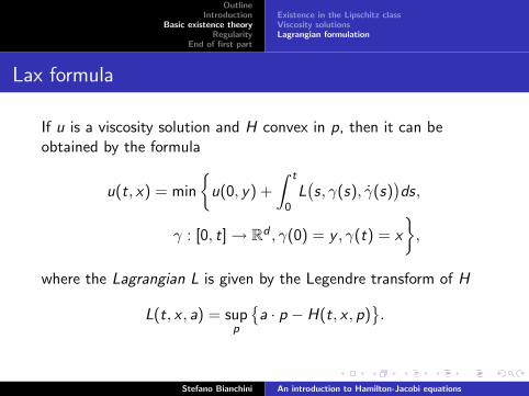
Lax formula
If u is a viscosity solution and H convex in p, then it can beobtained by the formula
u(t, x) = min
u(0, y) +
∫ t
0L(s, γ(s), γ(s)
)ds,
γ : [0, t]→ Rd , γ(0) = y , γ(t) = x
,
where the Lagrangian L is given by the Legendre transform of H
L(t, x , a) = supp
a · p − H(t, x , p)
.
Stefano Bianchini An introduction to Hamilton-Jacobi equations
OutlineIntroduction
Basic existence theoryRegularity
End of first part
Existence in the Lipschitz classViscosity solutionsLagrangian formulation
Lax formula
If u is a viscosity solution and H convex in p, then it can beobtained by the formula
u(t, x) = min
u(0, y) +
∫ t
0L(s, γ(s), γ(s)
)ds,
γ : [0, t]→ Rd , γ(0) = y , γ(t) = x
,
where the Lagrangian L is given by the Legendre transform of H
L(t, x , a) = supp
a · p − H(t, x , p)
.
Stefano Bianchini An introduction to Hamilton-Jacobi equations

OutlineIntroduction
Basic existence theoryRegularity
End of first part
Existence in the Lipschitz classViscosity solutionsLagrangian formulation
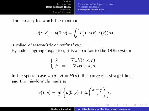
The curve γ for which the minimum
u(t, x) = u(0, y) +
∫ t
0L(s, γ(s), γ(s)
)ds
is called characteristic or optimal ray.
By Euler-Lagrange equation, it is a solution to the ODE systemx = ∇pH(t, x , p)p = −∇xH(t, x , p)
In the special case where H = H(p), this curve is a straight line,and the min-formula reads as
u(t, x) = infy
u(0, y) + tL
(x − y
t
).
Stefano Bianchini An introduction to Hamilton-Jacobi equations

OutlineIntroduction
Basic existence theoryRegularity
End of first part
Existence in the Lipschitz classViscosity solutionsLagrangian formulation
The curve γ for which the minimum
u(t, x) = u(0, y) +
∫ t
0L(s, γ(s), γ(s)
)ds
is called characteristic or optimal ray.By Euler-Lagrange equation, it is a solution to the ODE system
x = ∇pH(t, x , p)p = −∇xH(t, x , p)
In the special case where H = H(p), this curve is a straight line,and the min-formula reads as
u(t, x) = infy
u(0, y) + tL
(x − y
t
).
Stefano Bianchini An introduction to Hamilton-Jacobi equations
OutlineIntroduction
Basic existence theoryRegularity
End of first part
Some simple computationsA regularity resultRegularity for hyperbolic conservation laws
Outline
Introduction
Basic existence theory
RegularitySome simple computationsA regularity resultRegularity for hyperbolic conservation laws
End of first part
Stefano Bianchini An introduction to Hamilton-Jacobi equations
OutlineIntroduction
Basic existence theoryRegularity
End of first part
Some simple computationsA regularity resultRegularity for hyperbolic conservation laws
If H is convex in p, then the solution u is not only Lipschitz, butenjoys more regularity.
Example. Let H = p2/2, so that L = a2/2 and the function
x 7→ tL
(x − y
t
)=|x − y |2
2t
is semiconcave of parameter 1/t.Since the minimum of semiconcave functions is semiconcave, itfollows that the solution u to the HJ equation
∂tu +|∇xu|2
2= 0
is semiconcave.
Stefano Bianchini An introduction to Hamilton-Jacobi equations
OutlineIntroduction
Basic existence theoryRegularity
End of first part
Some simple computationsA regularity resultRegularity for hyperbolic conservation laws
If H is convex in p, then the solution u is not only Lipschitz, butenjoys more regularity.Example. Let H = p2/2, so that L = a2/2 and the function
x 7→ tL
(x − y
t
)=|x − y |2
2t
is semiconcave of parameter 1/t.
Since the minimum of semiconcave functions is semiconcave, itfollows that the solution u to the HJ equation
∂tu +|∇xu|2
2= 0
is semiconcave.
Stefano Bianchini An introduction to Hamilton-Jacobi equations
OutlineIntroduction
Basic existence theoryRegularity
End of first part
Some simple computationsA regularity resultRegularity for hyperbolic conservation laws
If H is convex in p, then the solution u is not only Lipschitz, butenjoys more regularity.Example. Let H = p2/2, so that L = a2/2 and the function
x 7→ tL
(x − y
t
)=|x − y |2
2t
is semiconcave of parameter 1/t.Since the minimum of semiconcave functions is semiconcave, itfollows that the solution u to the HJ equation
∂tu +|∇xu|2
2= 0
is semiconcave.
Stefano Bianchini An introduction to Hamilton-Jacobi equations
OutlineIntroduction
Basic existence theoryRegularity
End of first part
Some simple computationsA regularity resultRegularity for hyperbolic conservation laws
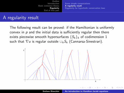
A regularity result
The following result can be proved: if the Hamiltonian is uniformlyconvex in p and the initial data is sufficiently regular then thereexists piecewise smooth hypersurfaces Skk of codimension 1such that ∇u is regular outside ∪kSk (Cannarsa-Sinestrari).
t
x
Stefano Bianchini An introduction to Hamilton-Jacobi equations
OutlineIntroduction
Basic existence theoryRegularity
End of first part
Some simple computationsA regularity resultRegularity for hyperbolic conservation laws
A regularity result
The following result can be proved: if the Hamiltonian is uniformlyconvex in p and the initial data is sufficiently regular then thereexists piecewise smooth hypersurfaces Skk of codimension 1such that ∇u is regular outside ∪kSk (Cannarsa-Sinestrari).
t
x
Stefano Bianchini An introduction to Hamilton-Jacobi equations

OutlineIntroduction
Basic existence theoryRegularity
End of first part
Some simple computationsA regularity resultRegularity for hyperbolic conservation laws
Due to the regularity outside the jumps of ∇xu, it is clear that thechange of variable
t = τ,x = γ(t, y),
y initial point of the characteristic γ,
is regular.
t
y
t
x
Stefano Bianchini An introduction to Hamilton-Jacobi equations
OutlineIntroduction
Basic existence theoryRegularity
End of first part
Some simple computationsA regularity resultRegularity for hyperbolic conservation laws
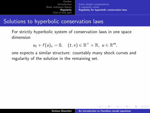
Solutions to hyperbolic conservation laws
For strictly hyperbolic system of conservation laws in one spacedimension
ut + f (u)x = 0, (t, x) ∈ R+ × R, u ∈ Rm,
one expects a similar structure: countably many shock curves andregularity of the solution in the remaining set.
x
t
Stefano Bianchini An introduction to Hamilton-Jacobi equations

OutlineIntroduction
Basic existence theoryRegularity
End of first part
Some simple computationsA regularity resultRegularity for hyperbolic conservation laws
Solutions to hyperbolic conservation laws
For strictly hyperbolic system of conservation laws in one spacedimension
ut + f (u)x = 0, (t, x) ∈ R+ × R, u ∈ Rm,
one expects a similar structure. However the presence of the othercharacteritic families generates a complicated structure.
x
t
Stefano Bianchini An introduction to Hamilton-Jacobi equations
OutlineIntroduction
Basic existence theoryRegularity
End of first part
Outline of the second partBibliography
Outline
Introduction
Basic existence theory
Regularity
End of first partOutline of the second partBibliography
Stefano Bianchini An introduction to Hamilton-Jacobi equations

OutlineIntroduction
Basic existence theoryRegularity
End of first part
Outline of the second partBibliography
In the second part of the talk we will be concerned with:
1. the structure of solutions if the initial data is only Lipschitzand H convex
2. the regularity of the decomposition of R+ × Rd given by thecharacteristics
3. the applications/extension of these results to conservationlaws and optimal transport on manifolds
Stefano Bianchini An introduction to Hamilton-Jacobi equations