CCS workshop, April 2013

An introduction to HYCOM

Matthieu Le Hénaff(1)

(1) RSMAS/CIMAS, Miami, FL

mlehenaff@rsmas.miami.edu

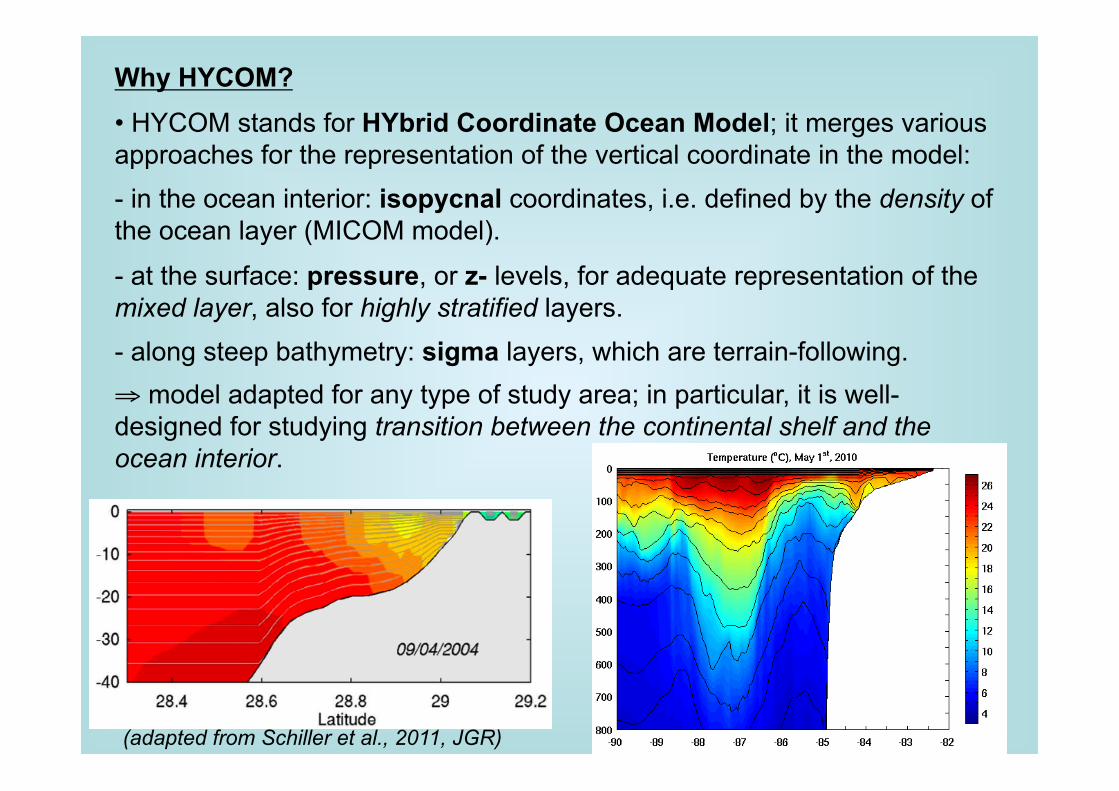
Why HYCOM?

•  HYCOM stands for HYbrid Coordinate Ocean Model; it merges various approaches for the representation of the vertical coordinate in the model: -  in the ocean interior: isopycnal coordinates, i.e. defined by the density of the ocean layer (MICOM model).

-  at the surface: pressure, or z- levels, for adequate representation of the mixed layer, also for highly stratified layers. -  along steep bathymetry: sigma layers, which are terrain-following. ⇒  model adapted for any type of study area; in particular, it is well-designed for studying transition between the continental shelf and the ocean interior.

(adapted from Schiller et al., 2011, JGR)

What do you need to run HYCOM?

•  Grid: based on the horizontal resolution chosen (1/12°, 1/25° etc.) •  Bathymetry: ETOPO, GEBCO etc…

•  Initial conditions: climatology, or output from another simulation. •  Forcing:

•  atmospheric conditions from climatology, or atmospheric model; •  river outflow from climatology or observations; •  photosynthetically available radiation coefficient, from satellite measurements (used for shortwave flux penetration).

•  Boundary conditions: relaxation to climatology, or nesting into another simulation.

But also…

•  Parameters for the model simulation and the multi-processing, and … a compiled model executable.

All these files are organized “rationally” on the computer.

Set-up of hycom directory

Main subdirectories:

•  ALL: toolbox to pre-process, or post-process files used for, or generated during the simulation •  •  various domains where one the model is run. Examples:

-  ATLb2.00 -  GOMl0.04 -  GLBa0.08 -  etc.

In these names: -  ATL means Atlantic, GOM means Gulf of Mexico, GLB mean global etc. -  the small letter is the version of the grid on the domain. -  the number following the root name is the horizontal resolution in degree: 2.00 is 2° resolution, 0.04 is 1/25° resolution etc.

Set-up of hycom directory

Within the domain subdirectories:

•  src: source directory for hycom code. Specific to a domain because the code needs information about the grid (and its decomposition for parallel computing) prior to compilation. Name typically extended to show version of the Hycom code used; example: src_2.2.18_20_mpi. •  •  config: contains files with compilation options, depending on the type of machine. •  •  topo: contains the grid and bathymetry information. •  •  relax: contains files for relaxation, at the boundaries or at the surface; usually based on climatology. •  •  nest: contains files for boundary conditions, in case of nesting. Based on another model simulation over a domain encompassing the study area. NB: Files in relax and nest have to be consistent with the grid configuration (spatial resolution, definition of vertical layers)

Set-up of hycom directory

•  force: contains forcing fields. Typical subdirectories: -  flux: fields used to calculate air-sea fluxes. -  pcip: precipitation. -  wind: wind speed and wind stress vectors. -  rivers: river outflow. -  seawifs: photosynthetically available radiation coefficient.

•  experiment directories: expt_01.0, ext_01.1, etc.

topo directory: grid and bathymetry files

•  regional.grid.a + regional.grid.b : grid •  regional.depth.a + regional.depth.b : bathymetry

NB: HYCOM files in a specific format, by pair: full data file *.a (binary), and header file *.b (in ascii).

•  •  regional.depth files usually have more specific name related to the grid: -  depth_GOMl0.04_71.[a,b] -  depth_ATLb2.00_01.[a,b] -  etc.

relax directory

•  relaxation fields used for: -  initial and/or boundary conditions in case of simulations based on climatology. -  surface relaxation in case of temperature or salinity relaxation needed.

•  files relax.temp.[a,b], relax.saln.[a,b] and nest_rmu.[a,b]

•  Typically use of monthly GDEM3 climatology + executables ‘z_gdem3’ and ‘relax_sig0’ or ‘relax_sig2’, in ~/hycom/ALL/relax/src/ to project fields on the specific HYCOM grid (horizontal and vertical interpolation). •  nest_rmu.[a,b] contains information on the buffer zone at the boundary (width and time-dependence). Created by ‘rmu’, in ~/hycom/ALL/relax/src

nest directory

•  contains archive fields with the same format, and on the same grid, as the specific HYCOM grid for the specified experiment: the fields are typically projected from a lower resolution, greater domain simulation. •  In case this outer simulation is HYCOM, the executable ‘isubregion’ in ~/hycom/ALL/subregion/src/ , to extract fields from the outer domain on the desired area, and project fields on the higher resolution grid.

force directory

•  atmospheric forcing: fields projected from an atmospheric model on the HYCOM horizontal grid. It includes:

•  in flux subdirectory, created with ‘ap’ in ~/hycom/ALL/force/src/ : -  airtmp.[a,b]: air temperature at the surface of the sea. -  radflx.[a,b]: radiative flux. -  shwflx.[a,b]: shortwave flux. -  vapmix.[a,b]: evaporation

•  in pcip, created with ‘ap’ in ~/hycom/ALL/force/src/ : -  pcip.[a,b]: precipition.

•  in wind, created with ‘wi’ in ~/hycom/ALL/force/src/ : -  wndspd.[a,b]: wind speed. -  tauewd.[a,b]: zonal wind stress. -  taunwd.[a,b]: meridional wind stress.

•  Variety of atmospheric models: NOGAPS, COAMPS, GFS etc.

force directory

•  river forcing: based on observations; climatology or actual data: -  monthly values: ‘pcip_riv_mon’ in ~/hycom/ALL/force/src/ -  daily values: ‘pcip_riv_hf’ in ~/hycom/ALL/force/src/

•  •  radiation coefficient: kpar.[a,b], based on monthly Seawifs observations, using ‘kp’ in ~/hycom/ALL/force/src/

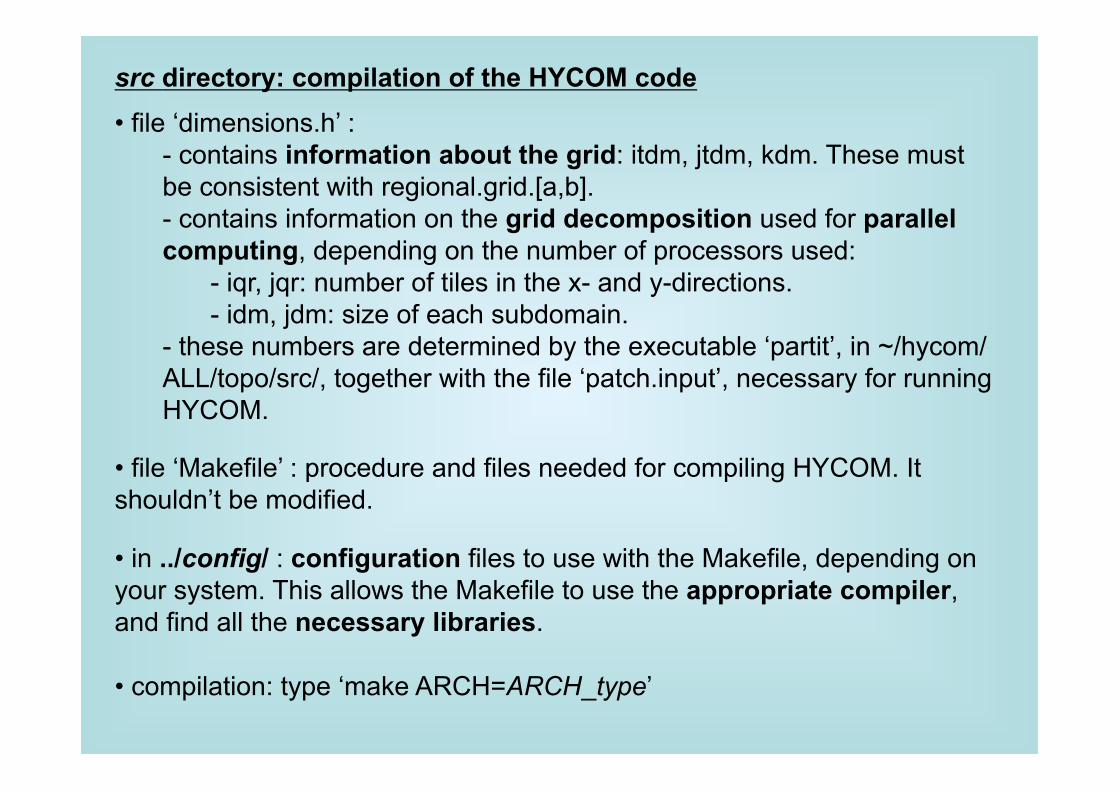
src directory: compilation of the HYCOM code

•  file ‘dimensions.h’ : -  contains information about the grid: itdm, jtdm, kdm. These must be consistent with regional.grid.[a,b]. -  contains information on the grid decomposition used for parallel computing, depending on the number of processors used:

-  iqr, jqr: number of tiles in the x- and y-directions. -  idm, jdm: size of each subdomain.

-  these numbers are determined by the executable ‘partit’, in ~/hycom/ALL/topo/src/, together with the file ‘patch.input’, necessary for running HYCOM.

•  file ‘Makefile’ : procedure and files needed for compiling HYCOM. It shouldn’t be modified.

•  in ../config/ : configuration files to use with the Makefile, depending on your system. This allows the Makefile to use the appropriate compiler, and find all the necessary libraries.

•  compilation: type ‘make ARCH=ARCH_type’

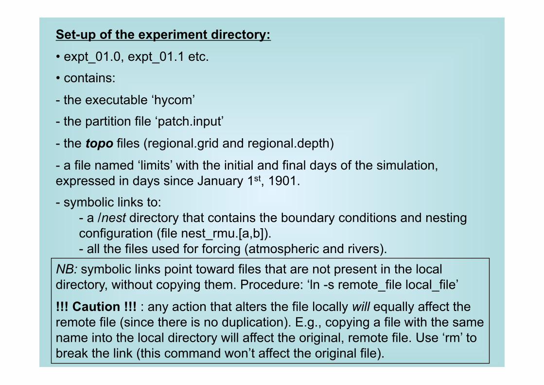
Set-up of the experiment directory: •  expt_01.0, expt_01.1 etc. •  contains:

-  the executable ‘hycom’ -  the partition file ‘patch.input’

-  the topo files (regional.grid and regional.depth)

-  a file named ‘limits’ with the initial and final days of the simulation, expressed in days since January 1st, 1901. -  symbolic links to:

-  a /nest directory that contains the boundary conditions and nesting configuration (file nest_rmu.[a,b]). -  all the files used for forcing (atmospheric and rivers).

NB: symbolic links point toward files that are not present in the local directory, without copying them. Procedure: ‘ln -s remote_file local_file’

!!! Caution !!! : any action that alters the file locally will equally affect the remote file (since there is no duplication). E.g., copying a file with the same name into the local directory will affect the original, remote file. Use ‘rm’ to break the link (this command won’t affect the original file).

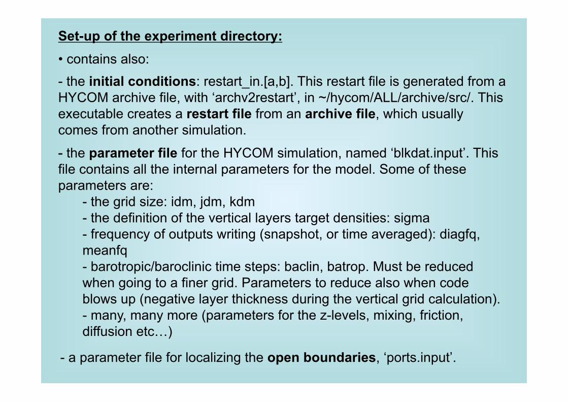
Set-up of the experiment directory:

•  contains also: -  the initial conditions: restart_in.[a,b]. This restart file is generated from a HYCOM archive file, with ‘archv2restart’, in ~/hycom/ALL/archive/src/. This executable creates a restart file from an archive file, which usually comes from another simulation.

-  -  the parameter file for the HYCOM simulation, named ‘blkdat.input’. This file contains all the internal parameters for the model. Some of these parameters are:

-  the grid size: idm, jdm, kdm -  the definition of the vertical layers target densities: sigma -  frequency of outputs writing (snapshot, or time averaged): diagfq, meanfq -  barotropic/baroclinic time steps: baclin, batrop. Must be reduced when going to a finer grid. Parameters to reduce also when code blows up (negative layer thickness during the vertical grid calculation). -  many, many more (parameters for the z-levels, mixing, friction, diffusion etc…)

-  a parameter file for localizing the open boundaries, ‘ports.input’.

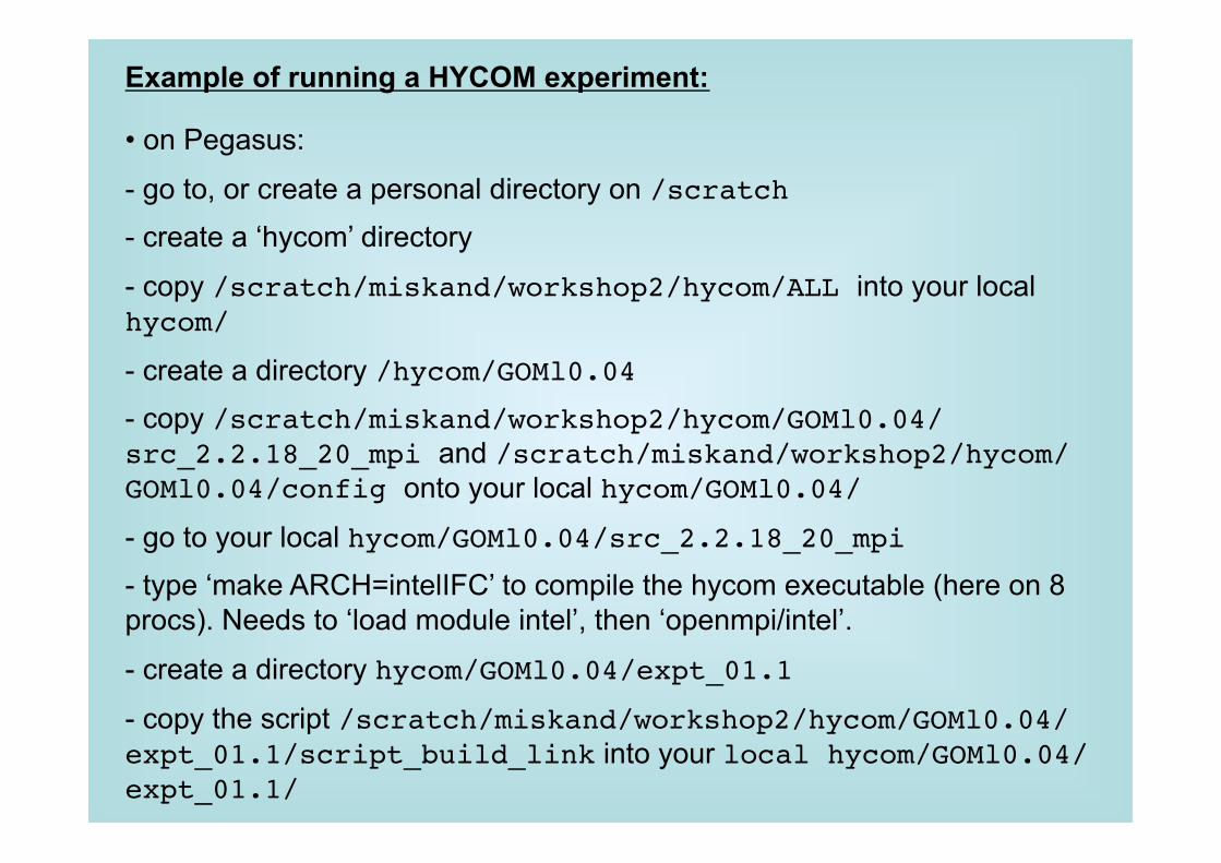
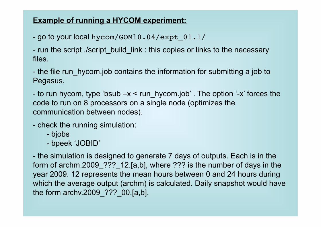
Example of running a HYCOM experiment:

•  on Pegasus:

-  go to, or create a personal directory on /scratch -  create a ‘hycom’ directory

-  copy /scratch/miskand/workshop2/hycom/ALL into your local hycom/

-  create a directory /hycom/GOMl0.04 -  copy /scratch/miskand/workshop2/hycom/GOMl0.04/src_2.2.18_20_mpi and /scratch/miskand/workshop2/hycom/GOMl0.04/config onto your local hycom/GOMl0.04/

-  go to your local hycom/GOMl0.04/src_2.2.18_20_mpi -  type ‘make ARCH=intelIFC’ to compile the hycom executable (here on 8 procs). Needs to ‘load module intel’, then ‘openmpi/intel’.

-  create a directory hycom/GOMl0.04/expt_01.1

-  copy the script /scratch/miskand/workshop2/hycom/GOMl0.04/expt_01.1/script_build_link into your local hycom/GOMl0.04/expt_01.1/

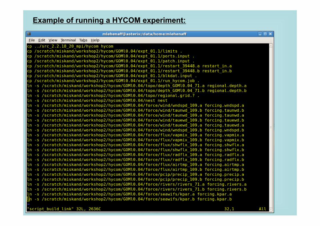
Example of running a HYCOM experiment:

Example of running a HYCOM experiment:

-  go to your local hycom/GOMl0.04/expt_01.1/

-  run the script ./script_build_link : this copies or links to the necessary files. -  the file run_hycom.job contains the information for submitting a job to Pegasus.

-  to run hycom, type ‘bsub –x < run_hycom.job’ . The option ‘-x’ forces the code to run on 8 processors on a single node (optimizes the communication between nodes).

-  check the running simulation: -  bjobs -  bpeek ‘JOBID’

-  the simulation is designed to generate 7 days of outputs. Each is in the form of archm.2009_???_12.[a,b], where ??? is the number of days in the year 2009. 12 represents the mean hours between 0 and 24 hours during which the average output (archm) is calculated. Daily snapshot would have the form archv.2009_???_00.[a,b].

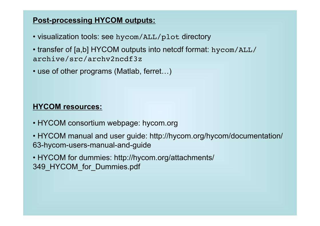
Post-processing HYCOM outputs:

•  visualization tools: see hycom/ALL/plot directory

•  transfer of [a,b] HYCOM outputs into netcdf format: hycom/ALL/archive/src/archv2ncdf3z •  use of other programs (Matlab, ferret…)

HYCOM resources:

•  HYCOM consortium webpage: hycom.org

•  HYCOM manual and user guide: http://hycom.org/hycom/documentation/63-hycom-users-manual-and-guide •  HYCOM for dummies: http://hycom.org/attachments/349_HYCOM_for_Dummies.pdf