Embed Size (px)
Citation preview
Introduction Numerical algorithms for nonsmooth optimization Conclusions References
An introduction to nonsmooth convexoptimization: numerical algorithms
Masoud Ahookhosh
Faculty of Mathematics, University of ViennaVienna, Austria
Convex Optimization I
January 29, 2014
1 / 35
Introduction Numerical algorithms for nonsmooth optimization Conclusions References
Table of contents
1 IntroductionDefinitionsApplications of nonsmooth convex optimizationBasic properties of subdifferential
2 Numerical algorithms for nonsmooth optimizationNonsmooth black-box optimizationProximal gradient algorithmSmoothing algorithmsOptimal complexity algorithms
3 Conclusions
4 References
2 / 35
Introduction Numerical algorithms for nonsmooth optimization Conclusions References
Definition of problems
Definition 1 (Structural convex optimization).
Consider the following a convex optimization problem
minimize f(x)subject to x ∈ C (1)
f(x) is a convex function;
C is a closed convex subset of vector space V ;
Properties:
f(x) can be smooth or nonsmooth;Solving nonsmooth convex optimization problems is much harderthan solving differentiable ones;For some nonsmooth nonconvex cases, even finding a decentdirection is not possible;The problem is involving linear operators. 3 / 35
Introduction Numerical algorithms for nonsmooth optimization Conclusions References
Applications
Applications of convex optimization:
Approximation and fitting;
Norm approximation;Least-norm problems;Regularized approximation;Robust approximation;Function fitting and interpolation;
Statistical estimation;
Parametric and nonparametric distribution estimation;Optimal detector design and hypothesis testing;Chebyshev and Chernoff bounds;Experiment design;
Global optimization;
Find bounds on the optimal value;Find approximation solutions;Convex relaxation;
4 / 35
Introduction Numerical algorithms for nonsmooth optimization Conclusions References
Geometric problems;
Projection on and distance between sets;Centering and classification;Placement and location;Smallest enclosed elipsoid;
Image and signal processing;
Optimizing the number of image models using convex relaxation;Image fusion for medical imaging;Image reconstruction;Sparse signal processing;
Design and control of complex systems;
Machine learning;
Financial and mechanical engineering;
Computational biology;
5 / 35
Introduction Numerical algorithms for nonsmooth optimization Conclusions References
Dfinition: subgradient and subdifferential
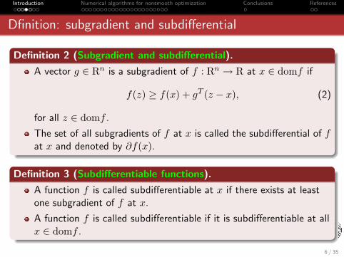
Definition 2 (Subgradient and subdifferential).
A vector g ∈ Rn is a subgradient of f : Rn → R at x ∈ domf if
f(z) ≥ f(x) + gT (z − x), (2)
for all z ∈ domf .
The set of all subgradients of f at x is called the subdifferential of fat x and denoted by ∂f(x).
Definition 3 (Subdifferentiable functions).
A function f is called subdifferentiable at x if there exists at leastone subgradient of f at x.
A function f is called subdifferentiable if it is subdifferentiable at allx ∈ domf .
6 / 35
Introduction Numerical algorithms for nonsmooth optimization Conclusions References
Subgradient and subdifferential
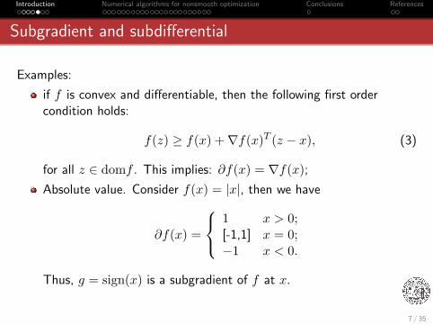
Examples:
if f is convex and differentiable, then the following first ordercondition holds:
f(z) ≥ f(x) +∇f(x)T (z − x), (3)
for all z ∈ domf . This implies: ∂f(x) = ∇f(x);
Absolute value. Consider f(x) = |x|, then we have
∂f(x) =
1 x > 0;[-1,1] x = 0;−1 x < 0.
Thus, g = sign(x) is a subgradient of f at x.
7 / 35
Introduction Numerical algorithms for nonsmooth optimization Conclusions References
Basic properties
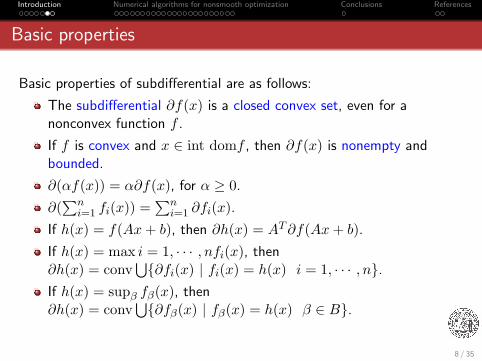
Basic properties of subdifferential are as follows:
The subdifferential ∂f(x) is a closed convex set, even for anonconvex function f .
If f is convex and x ∈ int domf , then ∂f(x) is nonempty andbounded.
∂(αf(x)) = α∂f(x), for α ≥ 0.
∂(∑n
i=1 fi(x)) =∑n
i=1 ∂fi(x).
If h(x) = f(Ax+ b), then ∂h(x) = AT∂f(Ax+ b).
If h(x) = max i = 1, · · · , nfi(x), then∂h(x) = conv
⋃{∂fi(x) | fi(x) = h(x) i = 1, · · · , n}.If h(x) = supβ fβ(x), then∂h(x) = conv
⋃{∂fβ(x) | fβ(x) = h(x) β ∈ B}.
8 / 35
Introduction Numerical algorithms for nonsmooth optimization Conclusions References
How to calculate subgradients
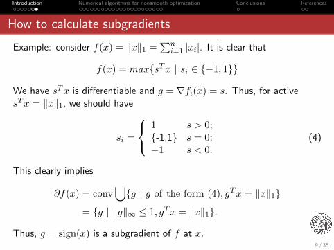
Example: consider f(x) = ‖x‖1 =∑n
i=1 |xi|. It is clear that
f(x) = max{sTx | si ∈ {−1, 1}}We have sTx is differentiable and g = ∇fi(x) = s. Thus, for activesTx = ‖x‖1, we should have
si =
1 s > 0;{-1,1} s = 0;−1 s < 0.
(4)
This clearly implies
∂f(x) = conv⋃{g | g of the form (4), gTx = ‖x‖1}
= {g | ‖g‖∞ ≤ 1, gTx = ‖x‖1}.Thus, g = sign(x) is a subgradient of f at x.
9 / 35
Introduction Numerical algorithms for nonsmooth optimization Conclusions References
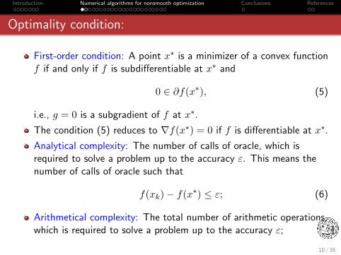
Optimality condition:
First-order condition: A point x∗ is a minimizer of a convex functionf if and only if f is subdifferentiable at x∗ and
0 ∈ ∂f(x∗), (5)
i.e., g = 0 is a subgradient of f at x∗.The condition (5) reduces to ∇f(x∗) = 0 if f is differentiable at x∗.Analytical complexity: The number of calls of oracle, which isrequired to solve a problem up to the accuracy ε. This means thenumber of calls of oracle such that
f(xk)− f(x∗) ≤ ε; (6)
Arithmetical complexity: The total number of arithmetic operations,which is required to solve a problem up to the accuracy ε;
10 / 35
Introduction Numerical algorithms for nonsmooth optimization Conclusions References
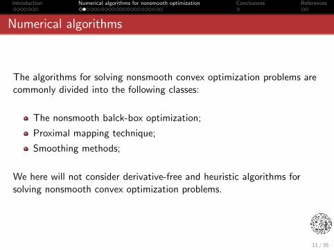
Numerical algorithms
The algorithms for solving nonsmooth convex optimization problems arecommonly divided into the following classes:
The nonsmooth balck-box optimization;
Proximal mapping technique;
Smoothing methods;
We here will not consider derivative-free and heuristic algorithms forsolving nonsmooth convex optimization problems.
11 / 35
Introduction Numerical algorithms for nonsmooth optimization Conclusions References
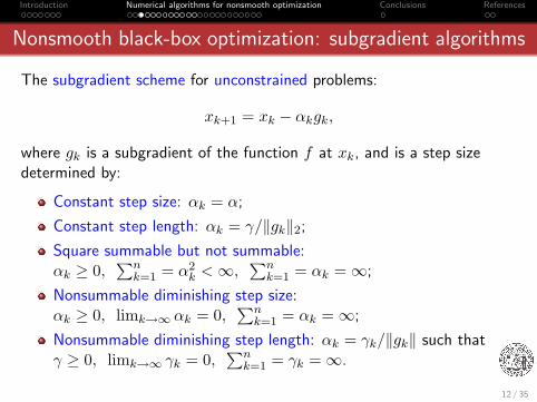
Nonsmooth black-box optimization: subgradient algorithms
The subgradient scheme for unconstrained problems:
xk+1 = xk − αkgk,
where gk is a subgradient of the function f at xk, and is a step sizedetermined by:
Constant step size: αk = α;
Constant step length: αk = γ/‖gk‖2;
Square summable but not summable:αk ≥ 0,
∑nk=1 = α2
k <∞,∑n
k=1 = αk =∞;
Nonsummable diminishing step size:αk ≥ 0, limk→∞ αk = 0,
∑nk=1 = αk =∞;
Nonsummable diminishing step length: αk = γk/‖gk‖ such thatγ ≥ 0, limk→∞ γk = 0,
∑nk=1 = γk =∞.
12 / 35
Introduction Numerical algorithms for nonsmooth optimization Conclusions References
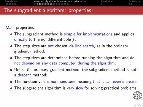
The subgradient algorithm: properties
Main properties:
The subgradient method is simple for implementations and appliesdirectly to the nondifferentiable f ;
The step sizes are not chosen via line search, as in the ordinarygradient method;
The step sizes are determined before running the algorithm and donot depend on any data computed during the algorithm;
Unlike the ordinary gradient method, the subgradient method is nota descent method;
The function vale is nonmonotone meaning that it can even increase;
The subgradient algorithm is very slow for solving practical problems.
13 / 35
Introduction Numerical algorithms for nonsmooth optimization Conclusions References
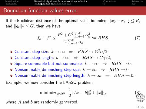
Bound on function values error:
If the Euclidean distance of the optimal set is bounded, ‖x0 − x∗‖2 ≤ R,and ‖gk‖2 ≤ G, then we have
fk − f∗ ≤ R2 +G2∑k
i=1 α2k
2∑k
i=1 αk:= RHS. (7)
Constant step size: k →∞ ⇒ RHS → G2α/2;
Constant step length: k →∞ ⇒ RHS → Gγ/2;
Square summable but not summable: k →∞ ⇒ RHS → 0;
Nonsummable diminishing step size: k →∞ ⇒ RHS → 0;
Nonsummable diminishing step length: k →∞ ⇒ RHS → 0.
Example: we now consider the LASSO problem
minimizex∈Rn12‖Ax− b‖22 + ‖x‖1, (8)
where A and b are randomly generated.14 / 35
Introduction Numerical algorithms for nonsmooth optimization Conclusions References
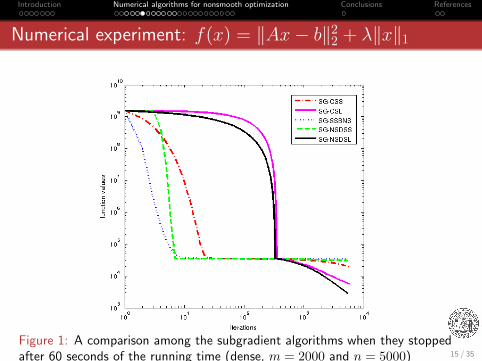
Numerical experiment: f(x) = ‖Ax− b‖22 + λ‖x‖1
Figure 1: A comparison among the subgradient algorithms when they stoppedafter 60 seconds of the running time (dense, m = 2000 and n = 5000) 15 / 35
Introduction Numerical algorithms for nonsmooth optimization Conclusions References
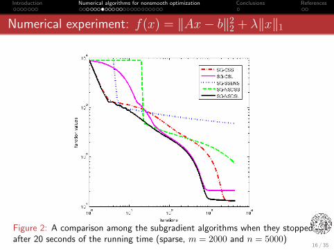
Numerical experiment: f(x) = ‖Ax− b‖22 + λ‖x‖1
Figure 2: A comparison among the subgradient algorithms when they stoppedafter 20 seconds of the running time (sparse, m = 2000 and n = 5000)
16 / 35
Introduction Numerical algorithms for nonsmooth optimization Conclusions References
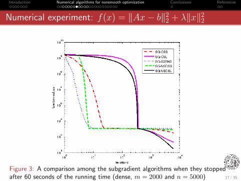
Numerical experiment: f(x) = ‖Ax− b‖22 + λ‖x‖22
Figure 3: A comparison among the subgradient algorithms when they stoppedafter 60 seconds of the running time (dense, m = 2000 and n = 5000) 17 / 35
Introduction Numerical algorithms for nonsmooth optimization Conclusions References
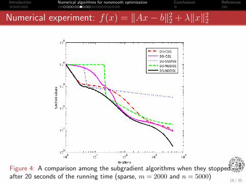
Numerical experiment: f(x) = ‖Ax− b‖22 + λ‖x‖22
Figure 4: A comparison among the subgradient algorithms when they stoppedafter 20 seconds of the running time (sparse, m = 2000 and n = 5000)
18 / 35
Introduction Numerical algorithms for nonsmooth optimization Conclusions References
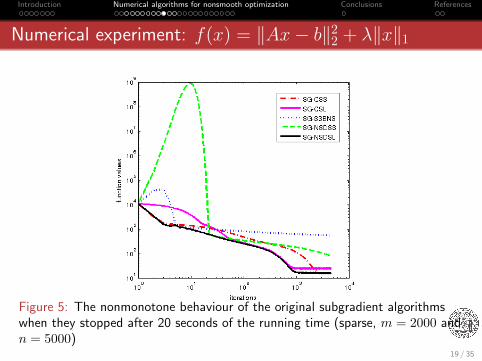
Numerical experiment: f(x) = ‖Ax− b‖22 + λ‖x‖1
Figure 5: The nonmonotone behaviour of the original subgradient algorithmswhen they stopped after 20 seconds of the running time (sparse, m = 2000 andn = 5000)
19 / 35
Introduction Numerical algorithms for nonsmooth optimization Conclusions References
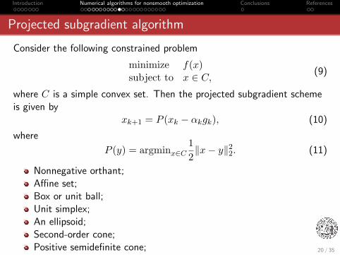
Projected subgradient algorithm
Consider the following constrained problem
minimize f(x)subject to x ∈ C, (9)
where C is a simple convex set. Then the projected subgradient schemeis given by
xk+1 = P (xk − αkgk), (10)
where
P (y) = argminx∈C12‖x− y‖22. (11)
Nonnegative orthant;Affine set;Box or unit ball;Unit simplex;An ellipsoid;Second-order cone;Positive semidefinite cone; 20 / 35
Introduction Numerical algorithms for nonsmooth optimization Conclusions References
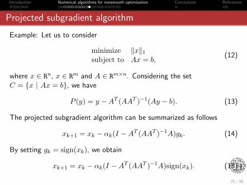
Projected subgradient algorithm
Example: Let us to consider
minimize ‖x‖1subject to Ax = b,
(12)
where x ∈ Rn, x ∈ Rm and A ∈ Rm×n. Considering the setC = {x | Ax = b}, we have
P (y) = y −AT (AAT )−1(Ay − b). (13)
The projected subgradient algorithm can be summarized as follows
xk+1 = xk − αk(I −AT (AAT )−1A)gk. (14)
By setting gk = sign(xk), we obtain
xk+1 = xk − αk(I −AT (AAT )−1A)sign(xk). (15)
21 / 35
Introduction Numerical algorithms for nonsmooth optimization Conclusions References
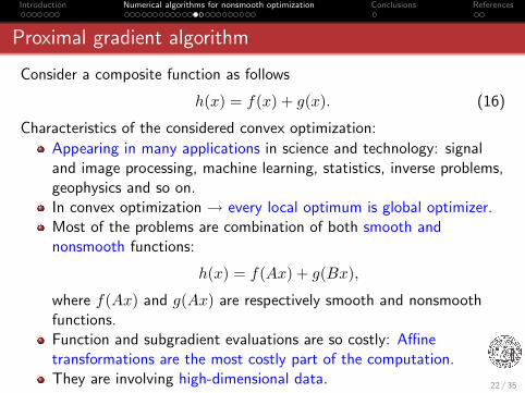
Proximal gradient algorithm
Consider a composite function as follows
h(x) = f(x) + g(x). (16)
Characteristics of the considered convex optimization:
Appearing in many applications in science and technology: signaland image processing, machine learning, statistics, inverse problems,geophysics and so on.In convex optimization → every local optimum is global optimizer.Most of the problems are combination of both smooth andnonsmooth functions:
h(x) = f(Ax) + g(Bx),
where f(Ax) and g(Ax) are respectively smooth and nonsmoothfunctions.Function and subgradient evaluations are so costly: Affinetransformations are the most costly part of the computation.They are involving high-dimensional data.
22 / 35
Introduction Numerical algorithms for nonsmooth optimization Conclusions References
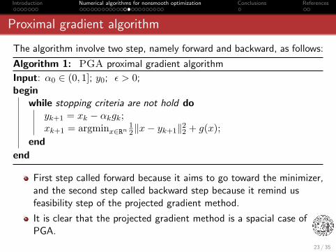
Proximal gradient algorithm
The algorithm involve two step, namely forward and backward, as follows:
Algorithm 1: PGA proximal gradient algorithm
Input: α0 ∈ (0, 1]; y0; ε > 0;begin
while stopping criteria are not hold doyk+1 = xk − αkgk;xk+1 = argminx∈Rn
12‖x− yk+1‖22 + g(x);
end
end
First step called forward because it aims to go toward the minimizer,and the second step called backward step because it remind usfeasibility step of the projected gradient method.
It is clear that the projected gradient method is a spacial case ofPGA.
23 / 35
Introduction Numerical algorithms for nonsmooth optimization Conclusions References
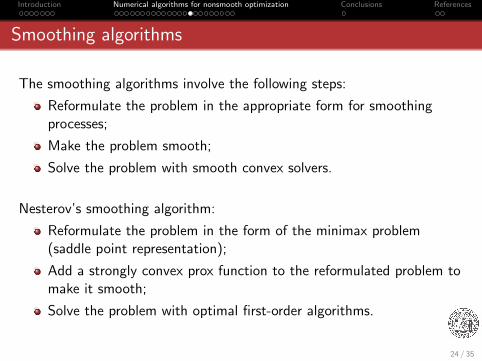
Smoothing algorithms
The smoothing algorithms involve the following steps:
Reformulate the problem in the appropriate form for smoothingprocesses;
Make the problem smooth;
Solve the problem with smooth convex solvers.
Nesterov’s smoothing algorithm:
Reformulate the problem in the form of the minimax problem(saddle point representation);
Add a strongly convex prox function to the reformulated problem tomake it smooth;
Solve the problem with optimal first-order algorithms.
24 / 35
Introduction Numerical algorithms for nonsmooth optimization Conclusions References
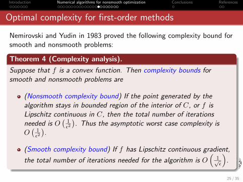
Optimal complexity for first-order methods
Nemirovski and Yudin in 1983 proved the following complexity bound forsmooth and nonsmooth problems:
Theorem 4 (Complexity analysis).
Suppose that f is a convex function. Then complexity bounds forsmooth and nonsmooth problems are
(Nonsmooth complexity bound) If the point generated by thealgorithm stays in bounded region of the interior of C, or f isLipschitz continuous in C, then the total number of iterationsneeded is O
(1ε2
). Thus the asymptotic worst case complexity is
O(
1ε2
).
(Smooth complexity bound) If f has Lipschitz continuous gradient,
the total number of iterations needed for the algorithm is O(
1√ε
).
25 / 35
Introduction Numerical algorithms for nonsmooth optimization Conclusions References
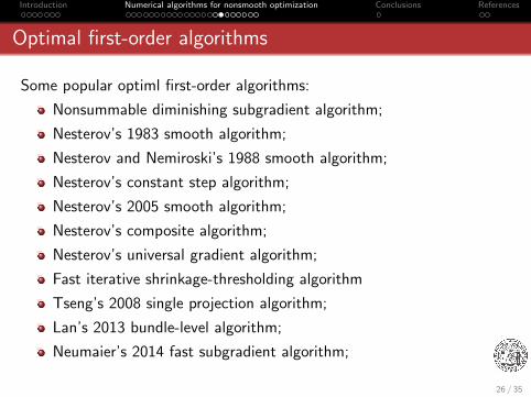
Optimal first-order algorithms
Some popular optiml first-order algorithms:
Nonsummable diminishing subgradient algorithm;
Nesterov’s 1983 smooth algorithm;
Nesterov and Nemiroski’s 1988 smooth algorithm;
Nesterov’s constant step algorithm;
Nesterov’s 2005 smooth algorithm;
Nesterov’s composite algorithm;
Nesterov’s universal gradient algorithm;
Fast iterative shrinkage-thresholding algorithm
Tseng’s 2008 single projection algorithm;
Lan’s 2013 bundle-level algorithm;
Neumaier’s 2014 fast subgradient algorithm;
26 / 35
Introduction Numerical algorithms for nonsmooth optimization Conclusions References
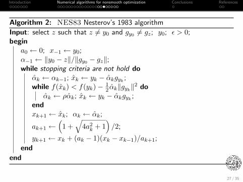
Algorithm 2: NES83 Nesterov’s 1983 algorithm
Input: select z such that z 6= y0 and gy0 6= gz; y0; ε > 0;begin
a0 ← 0; x−1 ← y0;α−1 ← ‖y0 − z‖/‖gy0 − gz‖;while stopping criteria are not hold do
α̂k ← αk−1; x̂k ← yk − α̂kgyk;
while f(x̂k) < f(yk)− 12 α̂k‖gyk
‖2 doα̂k ← ρα̂k; x̂k ← yk − α̂kgyk
;endxk+1 ← x̂k; αk ← α̂k;
ak+1 ←(1 +
√4a2
k + 1)/2;
yk+1 ← xk + (ak − 1)(xk − xk−1)/ak+1;
end
end
27 / 35
Introduction Numerical algorithms for nonsmooth optimization Conclusions References
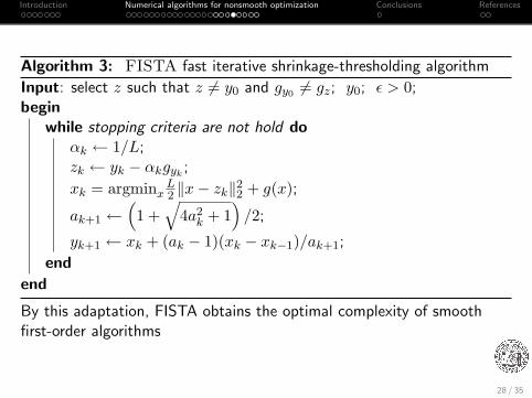
Algorithm 3: FISTA fast iterative shrinkage-thresholding algorithm
Input: select z such that z 6= y0 and gy0 6= gz; y0; ε > 0;begin
while stopping criteria are not hold doαk ← 1/L;zk ← yk − αkgyk
;
xk = argminxL2 ‖x− zk‖22 + g(x);
ak+1 ←(1 +
√4a2
k + 1)/2;
yk+1 ← xk + (ak − 1)(xk − xk−1)/ak+1;
end
end
By this adaptation, FISTA obtains the optimal complexity of smoothfirst-order algorithms
28 / 35
Introduction Numerical algorithms for nonsmooth optimization Conclusions References
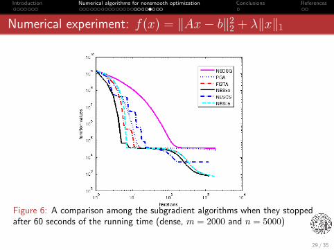
Numerical experiment: f(x) = ‖Ax− b‖22 + λ‖x‖1
Figure 6: A comparison among the subgradient algorithms when they stoppedafter 60 seconds of the running time (dense, m = 2000 and n = 5000)
29 / 35
Introduction Numerical algorithms for nonsmooth optimization Conclusions References
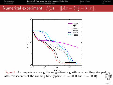
Numerical experiment: f(x) = ‖Ax− b‖22 + λ‖x‖1
Figure 7: A comparison among the subgradient algorithms when they stoppedafter 20 seconds of the running time (sparse, m = 2000 and n = 5000)
30 / 35
Introduction Numerical algorithms for nonsmooth optimization Conclusions References
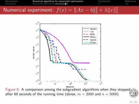
Numerical experiment: f(x) = ‖Ax− b‖22 + λ‖x‖22
Figure 8: A comparison among the subgradient algorithms when they stoppedafter 60 seconds of the running time (dense, m = 2000 and n = 5000)
31 / 35
Introduction Numerical algorithms for nonsmooth optimization Conclusions References
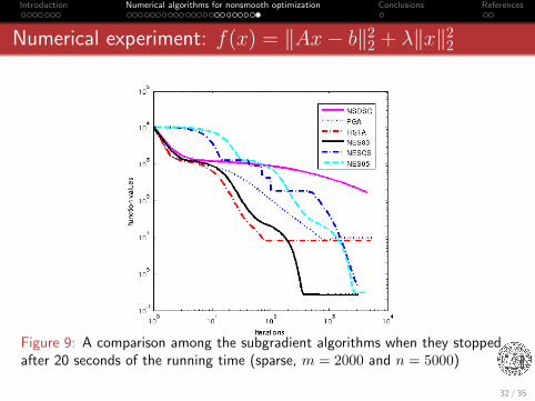
Numerical experiment: f(x) = ‖Ax− b‖22 + λ‖x‖22
Figure 9: A comparison among the subgradient algorithms when they stoppedafter 20 seconds of the running time (sparse, m = 2000 and n = 5000)
32 / 35
Introduction Numerical algorithms for nonsmooth optimization Conclusions References
Conclusions
Summarizing our discussion:
They are appearing in applications much more than smoothoptimization;Solving nonsmooth optimization problems is much harder thancommon smooth optimization;The most efficient algorithms for solving them are first-ordermethods;There are no normal stopping criterion in corresponding algorithms;The algorithms are divided into three classes:
Nonsmooth back-box algorithms;Proximal mapping algorithms;Smoothing algorithms;
Analytical complexity of the algorithms is the most important partof theoretical results;Optimal complexity algorithms are so efficient to solve practicalproblems.
33 / 35
Introduction Numerical algorithms for nonsmooth optimization Conclusions References
References
[1] Beck, A., Teboulle, M.: A fast iterative shrinkage-thresholdingalgorithm for linear inverse problems, SIAM Journal on ImagingSciences, 2 (2009), 183–202.
[2]Boyd, S., Xiao, L., Mutapcic, A.: Subgradient methods, (2003).
[3] Nemirovski, A.S., Yudin, D.: Problem Complexity and MethodEfficiency in Optimization. Wiley- Interscience Series in DiscreteMathematics. Wiley, XV (1983).
[4] Nesterov, Y.E.: Introductory Lectures on Convex Optimization: ABasic Course. Kluwer, Massachusetts (2004).
[5] Nesterov, Y.: A method of solving a convex programmingproblem with convergence rate O(1/k2), Doklady AN SSSR (InRussian), 269 (1983), 543-547. English translation: Soviet Math.Dokl. 27 (1983), 372–376.
34 / 35

Introduction Numerical algorithms for nonsmooth optimization Conclusions References
Thank you for your consideration
35 / 35
Introduction Novel optimal algorithms Numerical experiments Conclusions
Optimal subgradient methods for large-scaleconvex optimization
Masoud Ahookhosh
Faculty of Mathematics, University of ViennaVienna, Austria
Convex Optimization I
January 30, 2014
1 / 26
Introduction Novel optimal algorithms Numerical experiments Conclusions
Table of contents
1 IntroductionDefinition of the problemState-of-the-art solvers
2 Novel optimal algorithmsOptimal SubGradient Algorithm (OSGA)Algorithmic structure: OSGA
3 Numerical experimentsNumerical experiments: linear inverse problemComparison with state-of-the-art software
4 Conclusions
2 / 26
Introduction Novel optimal algorithms Numerical experiments Conclusions
Definition of problems
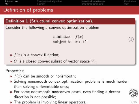
Definition 1 (Structural convex optimization).
Consider the following a convex optimization problem
minimize f(x)subject to x ∈ C (1)
f(x) is a convex function;
C is a closed convex subset of vector space V ;
Properties:
f(x) can be smooth or nonsmooth;Solving nonsmooth convex optimization problems is much harderthan solving differentiable ones;For some nonsmooth nonconvex cases, even finding a decentdirection is not possible;The problem is involving linear operators. 3 / 26
Introduction Novel optimal algorithms Numerical experiments Conclusions
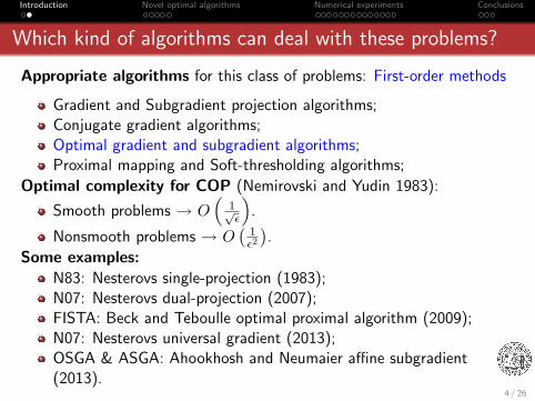
Which kind of algorithms can deal with these problems?
Appropriate algorithms for this class of problems: First-order methods
Gradient and Subgradient projection algorithms;Conjugate gradient algorithms;Optimal gradient and subgradient algorithms;Proximal mapping and Soft-thresholding algorithms;
Optimal complexity for COP (Nemirovski and Yudin 1983):
Smooth problems → O(
1√ε
).
Nonsmooth problems → O(
1ε2
).
Some examples:
N83: Nesterovs single-projection (1983);N07: Nesterovs dual-projection (2007);FISTA: Beck and Teboulle optimal proximal algorithm (2009);N07: Nesterovs universal gradient (2013);OSGA & ASGA: Ahookhosh and Neumaier affine subgradient(2013).
4 / 26
Introduction Novel optimal algorithms Numerical experiments Conclusions
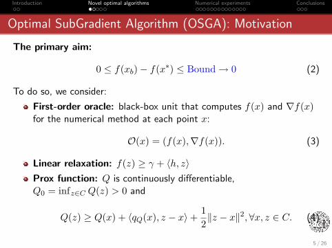
Optimal SubGradient Algorithm (OSGA): Motivation
The primary aim:
0 ≤ f(xb)− f(x∗) ≤ Bound→ 0 (2)
To do so, we consider:
First-order oracle: black-box unit that computes f(x) and ∇f(x)for the numerical method at each point x:
O(x) = (f(x),∇f(x)). (3)
Linear relaxation: f(z) ≥ γ + 〈h, z〉Prox function: Q is continuously differentiable,Q0 = infz∈C Q(z) > 0 and
Q(z) ≥ Q(x) + 〈qQ(x), z − x〉+12‖z − x‖2,∀x, z ∈ C. (4)
5 / 26
Introduction Novel optimal algorithms Numerical experiments Conclusions
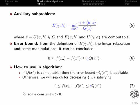
Auxiliary subproblem:
E(γ, h) = infz∈C
γ + 〈h, z〉Q(z)
(5)
where z = U(γ, h) ∈ C and E(γ, h) and U(γ, h) are computable.
Error bound: from the definition of E(γ, h), the linear relaxationand some manipulations, it can be concluded
0 ≤ f(xb)− f(x∗) ≤ ηQ(x∗). (6)
How to use in algorithm:If Q(x∗) is computable, then the error bound ηQ(x∗) is appliable.Otherwise, we will search for decreasing {ηk} satisfying
0 ≤ f(xb)− f(x∗) ≤ εQ(x∗). (7)
for some constant ε > 0.
6 / 26
Introduction Novel optimal algorithms Numerical experiments Conclusions
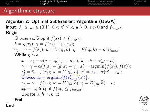
Algorithmic structure
Algoritm 2: Optimal SubGradient Algorithm (OSGA)Input: λ, αmax ∈ (0 1), 0 < κ′ ≤ κ, µ ≥ 0, ε > 0 and ftarget.Begin
Choose xb; Stop if f(xb) ≤ ftarget;h = g(xb); γ = f(xb)− 〈h, xb〉;γb = γ − f(xb); u = U(γb, h); η = E(γb, h)− µ; αmax;While η > ε
x = xb + α(u− xb); g = g(x); h̄ = h+ α(g − h);γ̄ = γ + α(f(x) + 〈g, x〉 − γ); x′b = argmin{f(xb), f(x)};γ′b = γ̄ − f(x′b); u′ = U(γ′b, h̄); x′ = xb + α(u′ − xb);Choose x̄b = argmin{f(x′b), f(x′)};γ̄b = γ̄ − f(x̄b); u′ = U(γ̄b, h̄); η = E(γ̄b, h̄)− µ;xb = x̄b; Stop if f(xb) ≤ ftarget;Update α, h, γ, η, u;
EndEnd
7 / 26
Introduction Novel optimal algorithms Numerical experiments Conclusions
Theoretical Analysis
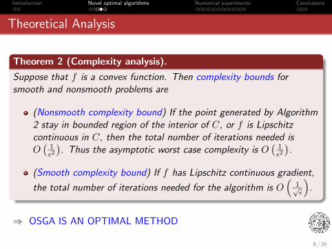
Theorem 2 (Complexity analysis).
Suppose that f is a convex function. Then complexity bounds forsmooth and nonsmooth problems are
(Nonsmooth complexity bound) If the point generated by Algorithm2 stay in bounded region of the interior of C, or f is Lipschitzcontinuous in C, then the total number of iterations needed isO(
1ε2
). Thus the asymptotic worst case complexity is O
(1ε2
).
(Smooth complexity bound) If f has Lipschitz continuous gradient,
the total number of iterations needed for the algorithm is O(
1√ε
).
⇒ OSGA IS AN OPTIMAL METHOD
8 / 26
Introduction Novel optimal algorithms Numerical experiments Conclusions
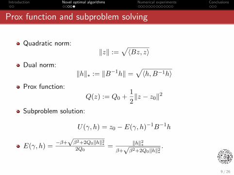
Prox function and subproblem solving
Quadratic norm:‖z‖ :=
√〈Bz, z〉
Dual norm:‖h‖∗ := ‖B−1h‖ =
√〈h,B−1h〉
Prox function:
Q(z) := Q0 +12‖z − z0‖2
Subproblem solution:
U(γ, h) = z0 − E(γ, h)−1B−1h
E(γ, h) = −β+√β2+2Q0‖h‖2∗2Q0
= ‖h‖2∗β+√β2+2Q0‖h‖2∗
.
9 / 26
Introduction Novel optimal algorithms Numerical experiments Conclusions
Numerical experiments: linear inverse problem
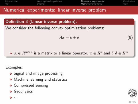
Definition 3 (Linear inverse problem).
We consider the following convex optimization problems:
Ax = b+ δ (8)
A ∈ Rm×n is a matrix or a linear operator, x ∈ Rn and b, δ ∈ Rm
Examples:
Signal and image processing
Machine learning and statistics
Compressed sensing
Geophysics
· · ·10 / 26
Introduction Novel optimal algorithms Numerical experiments Conclusions
Approximate solution
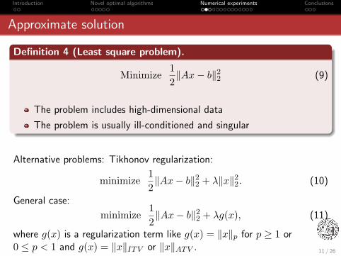
Definition 4 (Least square problem).
Minimize12‖Ax− b‖22 (9)
The problem includes high-dimensional data
The problem is usually ill-conditioned and singular
Alternative problems: Tikhonov regularization:
minimize12‖Ax− b‖22 + λ‖x‖22. (10)
General case:
minimize12‖Ax− b‖22 + λg(x), (11)
where g(x) is a regularization term like g(x) = ‖x‖p for p ≥ 1 or0 ≤ p < 1 and g(x) = ‖x‖ITV or ‖x‖ATV . 11 / 26
Introduction Novel optimal algorithms Numerical experiments Conclusions
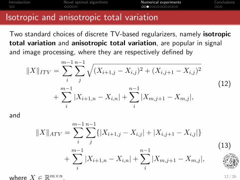
Isotropic and anisotropic total variation
Two standard choices of discrete TV-based regularizers, namely isotropictotal variation and anisotropic total variation, are popular in signaland image processing, where they are respectively defined by
‖X‖ITV =m−1∑i
n−1∑j
√(Xi+1,j −Xi,j)2 + (Xi,j+1 −Xi,j)2
+m−1∑i
|Xi+1,n −Xi,n|+n−1∑i
|Xm,j+1 −Xm,j |,(12)
and
‖X‖ATV =m−1∑i
n−1∑j
{|Xi+1,j −Xi,j |+ |Xi,j+1 −Xi,j |}
+m−1∑i
|Xi+1,n −Xi,n|+n−1∑i
|Xm,j+1 −Xm,j |,(13)
where X ∈ Rm×n. 12 / 26
Introduction Novel optimal algorithms Numerical experiments Conclusions
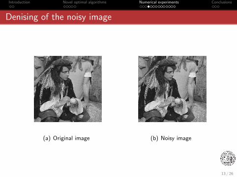
Denising of the noisy image
(a) Original image (b) Noisy image
13 / 26
Introduction Novel optimal algorithms Numerical experiments Conclusions
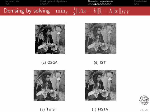
Denising by solving minx12‖Ax− b‖2
2 + λ‖x‖ITV
(c) OSGA (d) IST
(e) TwIST (f) FISTA
Figure 1: A comparison.
14 / 26
Introduction Novel optimal algorithms Numerical experiments Conclusions
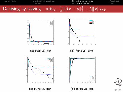
Denising by solving minx12‖Ax− b‖2
2 + λ‖x‖ITV
0 5 10 15 20 25 30 35 40 45 500
0.02
0.04
0.06
0.08
0.1
0.12
0.14
0.16
0.18
ISTTwISTFISTAOSGA
(a) step vs. iter
0 10 20 30 40 50 6010
−4
10−3
10−2
10−1
100
ISTTwISTFISTAOSGA
(b) Func vs. time
0 5 10 15 20 25 30 35 40 45 5010
−4
10−3
10−2
10−1
100
ISTTwISTFISTAOSGA
(c) Func vs. iter
0 5 10 15 20 25 30 35 40 45 500
1
2
3
4
5
6
7
8
ISTTwISTFISTAOSGA
(d) ISNR vs. iter
Figure 2: A comparison.
15 / 26
Introduction Novel optimal algorithms Numerical experiments Conclusions
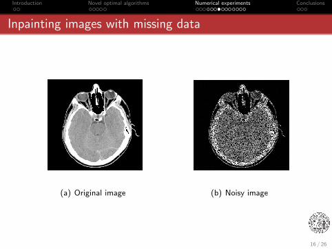
Inpainting images with missing data
(a) Original image (b) Noisy image
16 / 26
Introduction Novel optimal algorithms Numerical experiments Conclusions
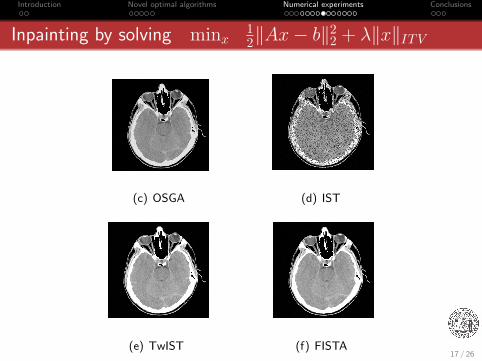
Inpainting by solving minx12‖Ax− b‖2
2 + λ‖x‖ITV
(c) OSGA (d) IST
(e) TwIST (f) FISTA
Figure 3: A comparison.
17 / 26
Introduction Novel optimal algorithms Numerical experiments Conclusions
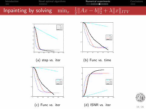
Inpainting by solving minx12‖Ax− b‖2
2 + λ‖x‖ITV
0 100 200 300 400 500 6000
0.1
0.2
0.3
0.4
0.5
0.6
0.7
ISTTwISTFISTAOSGA
(a) step vs. iter
0 10 20 30 40 50 6010
−3
10−2
10−1
100
ISTTwISTFISTAOSGA
(b) Func vs. time
0 100 200 300 400 500 60010
−3
10−2
10−1
100
ISTTwISTFISTAOSGA
(c) Func vs. iter
0 100 200 300 400 500 6000
5
10
15
20
25
ISTTwISTFISTAOSGA
(d) ISNR vs. iter
Figure 4: A comparison.
18 / 26
Introduction Novel optimal algorithms Numerical experiments Conclusions
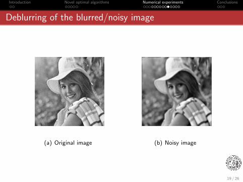
Deblurring of the blurred/noisy image
(a) Original image (b) Noisy image
19 / 26
Introduction Novel optimal algorithms Numerical experiments Conclusions
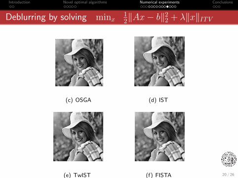
Deblurring by solving minx12‖Ax− b‖2
2 + λ‖x‖ITV
(c) OSGA (d) IST
(e) TwIST (f) FISTA
Figure 5: A comparison.
20 / 26
Introduction Novel optimal algorithms Numerical experiments Conclusions
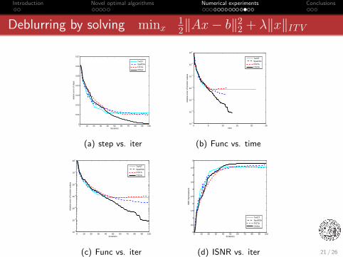
Deblurring by solving minx12‖Ax− b‖2
2 + λ‖x‖ITV
0 10 20 30 40 50 60 70 80 90 1000
0.01
0.02
0.03
0.04
0.05
0.06
0.07
iterations
rela
tive
erro
r of
ste
ps
TwISTSpaRSAFISTAOSGA
(a) step vs. iter
0 5 10 15 20 2510
−6
10−5
10−4
10−3
10−2
10−1
100
time
rela
tive
erro
r of
func
tion
valu
es
TwISTSpaRSAFISTAOSGA
(b) Func vs. time
0 10 20 30 40 50 60 70 80 90 10010
−6
10−5
10−4
10−3
10−2
10−1
100
iterations
rela
tive
erro
r of
func
tion
valu
es
TwISTSpaRSAFISTAOSGA
(c) Func vs. iter
0 10 20 30 40 50 60 70 80 90 1000
0.5
1
1.5
2
2.5
3
3.5
4
4.5
5
iterations
SN
R im
prov
emen
t
TwISTSpaRSAFISTAOSGA
(d) ISNR vs. iter
Figure 6: A comparison.
21 / 26
Introduction Novel optimal algorithms Numerical experiments Conclusions
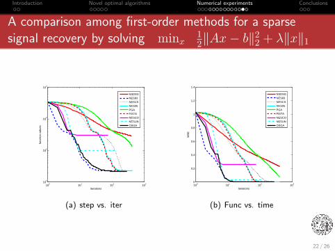
A comparison among first-order methods for a sparsesignal recovery by solving minx
12‖Ax− b‖2
2 + λ‖x‖1
100
101
102
103
101
102
103
104
iterations
func
tion
valu
es
NSDSGNES83NESCSNES05PGAFISTANESCONESUNOSGA
(a) step vs. iter
100
101
102
103
0
0.2
0.4
0.6
0.8
1
1.2
1.4
iterationsM
SE
NSDSGNES83NESCSNES05PGAFISTANESCONESUNOSGA
(b) Func vs. time
22 / 26
Introduction Novel optimal algorithms Numerical experiments Conclusions
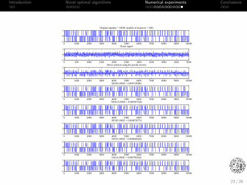
0 1000 2000 3000 4000 5000 6000 7000 8000 9000 10000−1
0
1Original signal(n = 10000, number of nonzeros = 300)
0 500 1000 1500 2000 2500 3000 3500 4000 4500 5000−1
0
1Noisy signal
0 1000 2000 3000 4000 5000 6000 7000 8000 9000 10000−1
0
1Direct solution using the pseudo inverse
0 1000 2000 3000 4000 5000 6000 7000 8000 9000 10000−1
0
1NES83 (MSE = 0.000729386)
0 1000 2000 3000 4000 5000 6000 7000 8000 9000 10000−1
0
1NESCS (MSE = 0.000947418)
0 1000 2000 3000 4000 5000 6000 7000 8000 9000 10000−1
0
1NES05 (MSE = 0.000870573)
0 1000 2000 3000 4000 5000 6000 7000 8000 9000 10000−1
0
1FISTA (MSE = 0.000849244)
0 1000 2000 3000 4000 5000 6000 7000 8000 9000 10000−1
0
1OSGA (MSE = 0.000796183)
23 / 26
Introduction Novel optimal algorithms Numerical experiments Conclusions
Conclusions and references
Summarizing our discussion:
OSGA is optimal algorithms for both smooth and nonsmooth convexoptimization problems;
OSGA is feasible and avoid using the Lipschitz information;
Low memory requirement OSGA makes them to be appropriate forsolving high-dimensional problems;
OSGA is efficient and robust in applications and practice andsuperior to some state-of-the-art solvers.
24 / 26
Introduction Novel optimal algorithms Numerical experiments Conclusions
References
[1] A. Neumaier, OSGA: fast subgradient algorithm with optimalcomplexity, Manuscript, University of Vienna, 2014.
[5] M. Ahookhosh, A. Neumaier, Optimal subgradient methods withapplication in large-scale linear inverse problems, Manuscript,University of Vienna, 2014.
[3] M. Ahookhosh, A. Neumaier, Optimal subgradient-basedmethods for convex constrained optimization I: theoretical results,Manuscript, University of Vienna, 2014.
[4] M. Ahookhosh, A. Neumaier, Optimal subgradient-basedmethods for convex constrained optimization II: numerical results,Manuscript, University of Vienna, 2014.
25 / 26

Introduction Novel optimal algorithms Numerical experiments Conclusions
Thank you for your consideration
26 / 26