Embed Size (px)
Citation preview
Structured Nonconvex and Nonsmooth Optimization:
Algorithms and Iteration Complexity Analysis
Bo Jiang ∗ Tianyi Lin † Shiqian Ma ‡ Shuzhong Zhang §
May 06, 2016
Abstract
Nonconvex and nonsmooth optimization problems are frequently encountered in muchof statistics, business, science and engineering, but they are not yet widely recognized as atechnology in the sense of scalability. A reason for this relatively low degree of popularity isthe lack of a well developed system of theory and algorithms to support the applications, asis the case for its convex counterpart. This paper aims to take one step in the direction ofdisciplined nonconvex and nonsmooth optimization. In particular, we consider in this papersome constrained nonconvex optimization models in block decision variables, with or withoutcoupled affine constraints. In the case of no coupled constraints, we show a sublinear rate ofconvergence to an ε-stationary solution in the form of variational inequality for a generalizedconditional gradient method, where the convergence rate is shown to be dependent on theHolderian continuity of the gradient of the smooth part of the objective. For the modelwith coupled affine constraints, we introduce corresponding ε-stationarity conditions, andpropose two proximal-type variants of the ADMM to solve such a model, assuming theproximal ADMM updates can be implemented for all the block variables except for the lastblock, for which either a gradient step or a majorization-minimization step is implemented.We show an iteration complexity bound of O(1/ε2) to reach an ε-stationary solution forboth algorithms. Moreover, we show that the same iteration complexity of a proximal BCDmethod follows immediately. Numerical results are provided to illustrate the efficacy of theproposed algorithms for tensor robust PCA.
Keywords: Structured Nonconvex Optimization, ε-Stationary Point, Iteration Complexity,Conditional Gradient Method, Alternating Direction Method of Multipliers, Block Coordi-nate Descent Method
Mathematics Subject Classification: 90C26, 90C06, 90C60
∗Research Center for Management Science and Data Analytics, School of Information Management and En-gineering, Shanghai University of Finance and Economics, Shanghai 200433, China. Research of this author wassupported in part by National Natural Science Foundation of China (Grant 11401364).†Research Center for Management Science and Data Analytics, School of Information Management and En-
gineering, Shanghai University of Finance and Economics, Shanghai 200433, China.‡Department of Systems Engineering and Engineering Management, The Chinese University of Hong Kong,
Shatin, N. T., Hong Kong. Research of this author was supported in part by the Hong Kong Research GrantsCouncil General Research Fund (Grant 14205314).§Department of Industrial and Systems Engineering, University of Minnesota, Minneapolis, MN 55455. Re-
search of this author was supported in part by the National Science Foundation (Grant CMMI-1462408).
1
1 Introduction
In this paper, we consider the following nonconvex and nonsmooth optimization problem withmultiple block variables:
min f(x1, x2, · · · , xN ) +N−1∑i=1
ri(xi)
s.t.∑N
i=1Aixi = b, xi ∈ Xi, i = 1, . . . , N − 1,
(1.1)
where f is differentiable and possibly nonconvex, and each ri is possibly nonsmooth and non-convex, i = 1, . . . , N − 1; Ai ∈ Rm×ni , b ∈ Rm, xi ∈ Rni ; and Xi ⊆ Rni are convex sets,i = 1, 2, . . . , N − 1. A special case of (1.1) is when the affine constraints are absent, and thereis no block structure of the variables, which leads to the following more compact form
min Φ(x) := f(x) + r(x), s.t. x ∈ S ⊂ Rn, (1.2)
where S is a convex and compact set. In this paper, we propose several first-order algorithmsfor computing an ε-stationary point (to be defined later) of (1.1) and (1.2), and analyze theiriteration complexities. Throughout this paper, we assume that the sets of the stationary pointsto (1.1) and (1.2) are non-empty.
Problem (1.1) arises from a variety of interesting applications. For example, one of thenonconvex models for matrix robust PCA can be casted as follows (see, e.g., [45]), which seeksto decompose a given matrix M ∈ Rm×n to a superposition of a low-rank matrix Z, a sparsematrix E and a noise matrix B:
minX,Y,Z,E,B ‖Z −XY >‖2F + αR(E)s.t. M = Z + E +B
‖B‖F ≤ η,(1.3)
where X ∈ Rm×r, Y ∈ Rn×r, with r < min(m,n) being the estimated rank of Z; η > 0 is thenoise level, α > 0 is a weighting parameter; R(E) is a regularization function that can improvethe sparsity of E. One of the widely used regularization functions is the `1 norm, which isconvex and nonsmooth. However, there are also many nonconvex regularization functions thatare widely used in statistical learning and information theory, such as smoothly clipped absolutedeviation (SCAD) [21], log-sum penalty (LSP) [15], minimax concave penalty (MCP) [50], andcapped-`1 penalty [51, 52], and they are nonsmooth at point 0 if composed with the absolutevalue function, which is usually the case in statistical learning. Clearly (1.3) is in the form of(1.1). Another example of the form (1.1) is the following nonconvex tensor robust PCA model(see, e.g., [48]), which seeks to decompose a given tensor T ∈ Rn1×n2×···×nd into a superpositionof a low-rank tensor Z, a sparse tensor E and a noise tensor B:
minXi,C,Z,E,B ‖Z − C ×1 X1 ×2 X2 ×3 · · · ×d Xd‖2F + αR(E)s.t. T = Z + E + B
‖B‖F ≤ η,(1.4)
where C is the core tensor that has smaller size than Z, and Xi are matrices with appropriatesizes, i = 1, . . . , d. In fact, the “low-rank” tensor in the above model corresponds to thetensor with a small core; however a recent work [32] demonstrates that the CP-rank of the coreregardless of its size could be as large as the original tensor. Therefore, if one wants to find thelow CP-rank decomposition, then the following model is preferred:
minXi,Z,E,B ‖Z − JX1, X2, · · · , XdK‖2 + αR(E) + ‖B‖2s.t. T = Z + E + B, (1.5)
2
for Xi = [ai,1, ai,2, · · · , ai,R] ∈ Rni×R, 1 ≤ i ≤ d and
JX1, X2, · · · , XdK :=R∑r=1
a1,r ⊗ a2,r ⊗ · · · ⊗ ad,r, (1.6)
where“⊗” denotes the outer product of vectors, and R is an estimation of the CP-rank. Inaddition, the so-called sparse tensor PCA problem [1], which seeks the best sparse rank-oneapproximation for a given d-th order tensor T , can also be formulated in the form of (1.1):
min −T (x1, x2, · · · , xd) + α∑d
i=1R(xi)s.t. xi ∈ Si = {x | ‖x‖22 ≤ 1}, i = 1, 2, . . . , d,
(1.7)
where T (x1, x2, · · · , xd) =∑
i1,...,idTi1,...,id(x1)i1 · · · (xd)id .
The convergence and iteration complexity for various nonconvex and nonsmooth optimiza-tion problems have recently attracted considerable research attention; see e.g. [3,6–8,10,11,19,24, 25, 38]. In this paper, we propose several solution methods that use only the first-order in-formation of the objective function, including generalized conditional gradient method, variantsof alternating direction method of multipliers, and proximal block coordinate descent method,for solving (1.1) and (1.2). Specifically, we propose a generalized conditional gradient (GCG)method for solving (1.2). We prove that GCG can find an ε-stationary point for (1.2) in O(ε−q)iterations under certain mild conditions, where q is a parameter in the Holder condition thatcharacterizes the degree of smoothness of f . In other words, the speed of the algorithm’s con-vergence depends on the degree of “smoothness” of the objective function. It should be notedthat a similar iteration bound that depends on the parameter q was only recently reported inthe context of convex optimization [13]. Furthermore, we show that if f is concave, then GCGfinds an ε-stationary point for (1.2) in O(1/ε) iterations. For the affinely constrained problem(1.1), we propose two algorithms (called proximal ADMM-g and proximal ADMM-m in thispaper) that can both be viewed as variants of the alternating direction method of multipliers(ADMM). Recently, there have been some emerging interests on the ADMM for nonconvexproblems (see, e.g., [2, 29, 30, 35, 46, 47, 49]). The results in [35, 46, 47, 49] only proved the con-vergence of ADMM to a stationary point, and no iteration complexity analysis was provided.Moreover, the objective function is required to satisfy the so-called Kurdyka- Lojasiewicz (KL)property [9, 33, 39, 40] to ensure those convergence results. In [30], Hong, Luo and Razaviyaynanalyzed the convergence of ADMM for solving nonconvex consensus and sharing problems.Note that they also analyzed the iteration complexity of ADMM for the consensus problem.However, they require the nonconvex part of the objective function to be smooth, and nons-mooth part to be convex. In contrast, ri in our model (1.1) can be nonconvex and nonsmoothat the same time. Moreover, we allow general set constraints xi ∈ Xi, i = 1, . . . , N−1, while theconsensus problem in [30] only allows the set constraint for one block variable. The very recentwork by Hong [29] discusses the iteration complexity of an augmented Lagrangian method forfinding an ε-stationary point for the following problem:
min f(x), s.t. Ax = b, x ∈ Rn, (1.8)
under the assumption that f is differentiable. We will compare our results with [29] in moredetails in Section 3.
Throughout this paper, we make the following assumption.
Assumption 1.1 All subproblems in our algorithms, though possibly nonconvex, can be solvedto global optimality.
We shall show later that the solvability of our subproblems usually boils down to the com-putability of the proximal mapping with respect to the nonsmooth part of the objective function.
3
Besides, the proximal mappings of the aforementioned nonsmooth regularization functions, in-cluding the `1 norm, SCAD, LSP, MCP and Capped-`1 penalty, all admit closed-form solutions,and the explicit formulae can be found in [26].
Before proceeding, let us first summarize:
Our contributions.
(i) We provide a systematic study on how to define an ε-stationary point of (1.1) and (1.2).For (1.1), our definition of ε-stationary point covers the cases when each ri is convex, orri is Lipschitz continuous (possibly nonconvex), or ri is lower semi-continuous (possiblynonconvex).
(ii) We propose a generalized conditional gradient method for solving (1.2) and analyze itsiteration complexity for obtaining an ε-stationary point of (1.2).
(iii) We propose two ADMM variants (proximal ADMM-g and proximal ADMM-m) for solving(1.1), under certain conditions on AN . We also analyze their iteration complexities forobtaining an ε-stationary point of (1.1).
(iv) As an extension, we also show how to use proximal ADMM-g and proximal ADMM-m tofind an ε-stationary point of (1.1) without assuming any assumption on AN .
(v) As a by-product, we also propose a proximal block coordinate descent (BCD) methodwith cyclic order for solving (1.1) when the affine constraints are absent, and show thatits iteration complexity can be obtained directly from that of proximal ADMM-g andproximal ADMM-m.
Notation. We use ‖x‖2 to denote the Euclidean norm of vector x, and ‖x‖2H to denotex>Hx for some positive definite matrix H. For set S and scalar p > 1, we denote
diamp(S) := maxx,y ∈S
‖x− y‖p, (1.9)
where ‖x‖p = (∑n
i=1 |xi|p)1/p. Without specification, we denote ‖x‖ = ‖x‖2 and diam(S) =diam2(S) for short. We use dist(x, S) to denote the Euclidean distance of vector x to set S.Given a matrix A, its spectral norm, largest singular value and smallest singular value aredenoted by ‖A‖2, σmax(A) and σmin(A) respectively. We use dae to denote the largest integerthat is less than or equal to scalar a.
Organization. The rest of this paper is organized as follows. In Section 2 we give thedefinition of ε-stationary point of (1.2) and propose a generalized conditional gradient methodthat solves (1.2) and analyze its iteration complexity for obtaining such an ε-stationary point of(1.2). In Section 3 we give three definitions of ε-stationarity for (1.1) under different settings andpropose two ADMM variants that solve (1.1) and analyze their iteration complexities to reachan ε-stationary point of (1.1). In Section 4 we provide some extensions of the results in Section3. In particular, we first show how to remove some of the conditions that we assume in Section3, and then we propose a proximal BCD method to solve (1.1) without affine constraints andprovide an iteration complexity analysis. In Section 5, we provide numerical results to illustratethe practical efficiency of the proposed algorithms.
2 A generalized conditional gradient method
In this section, we propose a GCG method for solving (1.2) and analyze its iteration com-plexity. The conditional gradient (CG) method, also known as the Frank-Wolfe method, was
4
originally proposed in [22], and regained a lot of popularity recently due to its capability ofsolving large-scale problems (see, [4,5,23,27,31,34,42]). However, these works focus on solvingconvex problems. Bredies et al. [14] considered a generalized conditional gradient method forsolving nonconvex problems in Hilbert space, which is similar to our algorithm, but no iterationcomplexity was provided.
Throughout this section, we make the following assumption regarding to problem (1.2).
Assumption 2.1 In (1.2), function r(x) is convex and nonsmooth, and the constraint set S isconvex and compact. Moreover, f is differentiable and there exist some p > 1 and ρ > 0 suchthat
f(y) ≤ f(x) +∇f(x)>(y − x) +ρ
2‖y − x‖pp, ∀x, y ∈ S. (2.1)
The inequality (2.1) is the so-called Holder condition and was also used in other papersthat discuss first-order algorithms (e.g., [20]). It can be shown that (2.1) holds for a variety offunctions. In fact, we have the following results.
Proposition 2.2
(i) If f is concave, then (2.1) holds for any p > 0 and ρ > 0.
(ii) If the gradient of f satisfies
‖∇f(x)−∇f(y)‖qq ≤M‖x− y‖pp, ∀ x, y ∈ S, (2.2)
for some M > 0, 1 < p ≤ 2 and 1p + 1
q = 1, then (2.1) holds.
(iii) (2.1) holds for the p-norm function
f(x) =n∑i=1
xpi , where 1 < p ≤ 2 and xi > 0, i = 1, . . . , n. (2.3)
Proof. Part (i) is obvious. For (ii), let z = y − x and g(α) = f(x+ αz), it follows that
f(y)− f(x) =
∫ 1
0g′(α)z dα =
∫ 1
0∇f(x+ αz)>z dα
≤ ∇f(x)>z +
∣∣∣∣∫ 1
0(∇f(x+ αz)−∇f(x))>z dα
∣∣∣∣≤ ∇f(x)>z +
∫ 1
0‖∇f(x+ αz)−∇f(x)‖q‖z‖p dα
≤ ∇f(x)>z +M1/q‖z‖1+ p
qp
∫ 1
0αpq dα
= ∇f(x)>z +M1/q
p‖z‖pp,
where the last equality is due to 1p + 1
q = 1. Thus, the function with Lipschitz continuousgradient automatically satisfies inequality (2.1) for p = q = 2. In fact, condition (2.2) reflectsthe degree of the Holderian continuity of ∇f , which was also considered in [20] to construct aso-called inexact first-order oracle. For Part (iii), we observe that the function is separable withrespect to all xi, so it suffices to show that there exists some ρ such that:
vp ≤ up + (up)′(v − u) +ρ
2|v − u|p = up + p up−1(v − u) +
ρ
2|v − u|p, (2.4)
5
when 1 < p ≤ 2. If u = 0, then the inequality trivially holds for any ρ ≥ 2; otherwise we candivide both sides by |u|p and aim to prove an equivalent formulation:
kp ≤ 1 + p(k − 1) +ρ
2|k − 1|p, (2.5)
where k = v/u. To this end, define
g(k) :=
{0 if k = 1
kp−1−p(k−1)|k−1|p otherwise.
Observe that limk→+∞
g(k) = 1 and by the L’Hospital rule
limk→1
g(k) =
{0 if 1 < p < 21 if p = 2,
so g(k) is upper bounded on R and there exits some ρ such that (2.5) holds. Finally by lettingρ = max{2, ρ}, the inequality (2.4) follows. �
2.1 An ε-stationary point for problem (1.2)
Our definition of an ε-stationary point of (1.2) is given as follows.
Definition 2.3 We call x to be an ε-stationary point (ε ≥ 0) of (1.2) if the following mixedvariational inequality conditions is satisfied:
ψS(x) := ∇f(x)>(y − x) + r(y)− r(x) ≥ −ε, ∀y ∈ S. (2.6)
If ε = 0, we call x to be a stationary point of (1.2).
When ε = 0, the condition (2.6) is stronger than the commonly used KKT condition in thesense that it is a necessary condition for local minimum of (1.2). To see this, suppose that thereexists some y ∈ S such that ∇f(x)>(y − x) + r(y) − r(x) < 0. Denote d = y − x. Then thedirectional derivative along direction d at point x satisfies
(f + r)′(x; d) = limα↘0
f(x+ αd) + r(x+ αd)− f(x)− r(x)
α
≤ limα↘0
f(x+ αd)− f(x)
α+ limα↘0
(1− α)r(x) + αr(x+ d)− r(x)
α
= ∇f(x)>(y − x) + r(y)− r(x) < 0,
where the first inequality is due to the convexity of r. As a result, x cannot be a local minimizerof problem (1.2).
We now compare our Definition 2.3 with some existing definitions of ε-stationary point inthe literature. For the smooth unconstrained problem {min f(x)}, it is natural to define theε-stationary point using the criterion ‖∇f(x)‖2 ≤ ε. Nesterov [43] and Cartis et al. [17] showedthat the gradient descent type methods with properly chosen step size need O(1/ε2) iterationsto find such a point. Moreover, Cartis et al. [16] constructed an example showing that theO(1/ε2) iteration complexity is tight for the steepest descent type algorithm. However, the casefor the constrained nonconvex optimization is more complicated. When r ≡ 0 in (1.2), i.e., theobjective function is differentiable, Cartis et al. [18] proposed the following measure:
χS(x) :=
∣∣∣∣ minx+d∈S,‖d‖2≤1
∇f(x)>d
∣∣∣∣ ≤ ε. (2.7)
6
They showed that it requires no more than O(1/ε2) iterations for the adaptive cubic regular-ization algorithm in [18] to find an x satisfying (2.7). Ghadimi et al. [25] gave the followingdefinition of an ε-stationary point of (1.2). Define
PS(x, γ) :=1
γ(x− x+), where x+ = arg min
y∈S∇f(x)>y +
1
γV (y, x) + r(y), (2.8)
where γ > 0 and V is a prox-function. Ghadimi et al. [25] proposed a projected gradientalgorithm to solve (1.2) and proved that it takes no more than O(1/ε2) iterations to find an xsatisfying
‖PS(x, γ)‖22 ≤ ε. (2.9)
We have the following proposition regarding the relationships among the three definitionsof ε-stationary point defined in (2.6), (2.7) and (2.9).
Proposition 2.4 Consider (1.2).
(i) When r(x) ≡ 0, if ψS(x) ≥ −ε, then χS(x) ≤ ε;
(ii) Suppose that the prox-function V (y, x) = ‖y−x‖22/2, then ψS(x) ≥ −ε implies ‖PS(x, γ)‖22 ≤ε/γ. Conversely, if we further assume that the gradient function ∇f(x) is continuous, then‖PS(x, γ)‖22 ≤ ε implies
ψS(x) ≥ −(γ τ + γ ς + diam(S))√ε, (2.10)
where τ = maxx∈S ‖∇f(x)‖2, ς = maxx∈S minz∈∂r(x) ‖z‖2. Note that ς is finite, becauseS is compact.
Proof. Part (i) follows from (2.6) and (2.7) by the following relationships:
ψS(x) ≥ −ε =⇒ ∇f(x)>(y − x) ≥ −ε,∀ ‖y − x‖2 ≤ 1, y ∈ S=⇒ 0 ≥ min
x+d∈S,‖d‖2≤1∇f(x)>d ≥ −ε =⇒ χS(x) ≤ ε.
We now prove part (ii). Since V (y, x) = ‖y − x‖22/2, (2.8) implies that(∇f(x) +
1
γ(x+ − x) + z
)>(y − x+) ≥ 0, ∀ y ∈ S, (2.11)
where z ∈ ∂r(x+). By choosing y = x in (2.11) one can get
∇f(x)>(x− x+) + r(x)− r(x+) ≥ (∇f(x) + z)> (x− x+) ≥ 1
γ‖x+ − x‖22. (2.12)
Therefore, if ψS(x) ≥ −ε, then ‖PS(x, γ)‖22 ≤ εγ holds. To show the other direction, note that
for x, x+ ∈ S, one can choose w ∈ ∂r(x) such that
ς ‖x− x+‖2 ≥ w>(x− x+) ≥ r(x)− r(x+),
which together with (2.12) implies that
∇f(x)>(y − x) + r(y)− r(x) + (‖∇f(x)‖2 + ς)‖x− x+‖2≥ ∇f(x)>(y − x) + r(y)− r(x) +∇f(x)>(x− x+) + r(x)− r(x+)
= ∇f(x)>(y − x+) + r(y)− r(x+)
≥ (∇f(x) + z)> (y − x+) ≥ −1
γ(x+ − x)>(y − x+) ≥ −1
γ‖y − x+‖2‖x+ − x‖2, ∀y ∈ S,
7
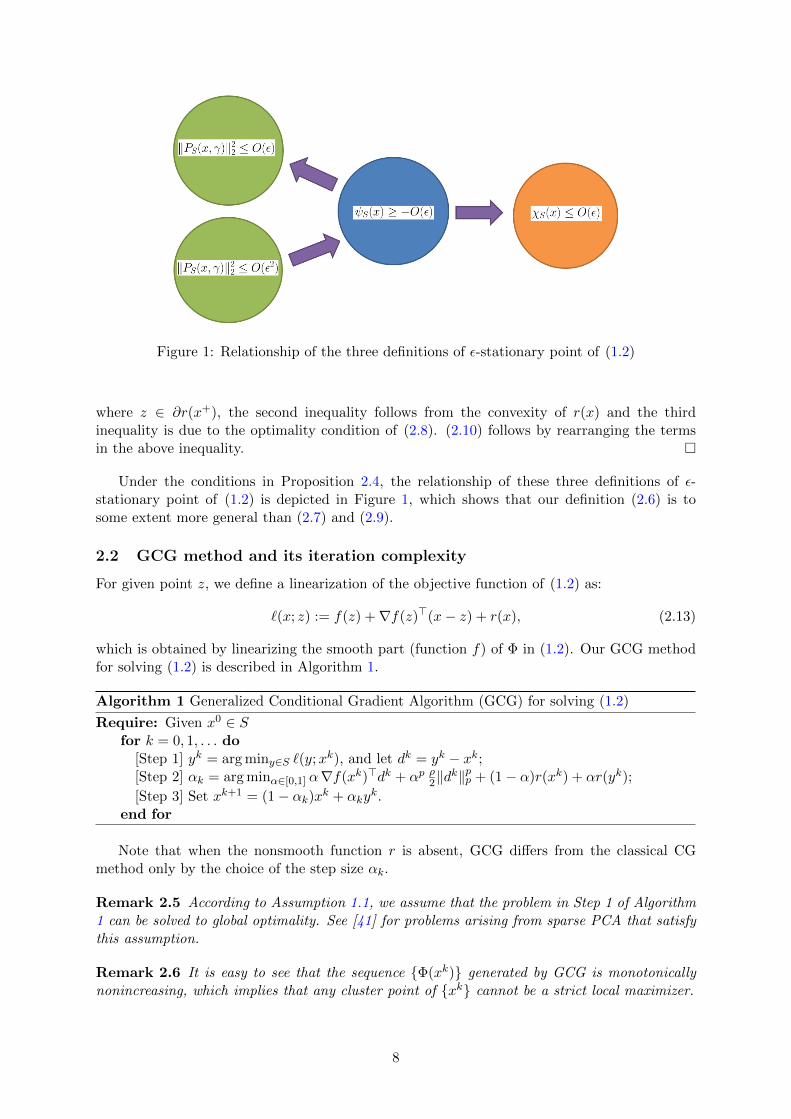
Figure 1: Relationship of the three definitions of ε-stationary point of (1.2)
where z ∈ ∂r(x+), the second inequality follows from the convexity of r(x) and the thirdinequality is due to the optimality condition of (2.8). (2.10) follows by rearranging the termsin the above inequality. �
Under the conditions in Proposition 2.4, the relationship of these three definitions of ε-stationary point of (1.2) is depicted in Figure 1, which shows that our definition (2.6) is tosome extent more general than (2.7) and (2.9).
2.2 GCG method and its iteration complexity
For given point z, we define a linearization of the objective function of (1.2) as:
`(x; z) := f(z) +∇f(z)>(x− z) + r(x), (2.13)
which is obtained by linearizing the smooth part (function f) of Φ in (1.2). Our GCG methodfor solving (1.2) is described in Algorithm 1.
Algorithm 1 Generalized Conditional Gradient Algorithm (GCG) for solving (1.2)
Require: Given x0 ∈ Sfor k = 0, 1, . . . do
[Step 1] yk = arg miny∈S `(y;xk), and let dk = yk − xk;[Step 2] αk = arg minα∈[0,1] α∇f(xk)>dk + αp ρ2‖d
k‖pp + (1− α)r(xk) + αr(yk);
[Step 3] Set xk+1 = (1− αk)xk + αkyk.
end for
Note that when the nonsmooth function r is absent, GCG differs from the classical CGmethod only by the choice of the step size αk.
Remark 2.5 According to Assumption 1.1, we assume that the problem in Step 1 of Algorithm1 can be solved to global optimality. See [41] for problems arising from sparse PCA that satisfythis assumption.
Remark 2.6 It is easy to see that the sequence {Φ(xk)} generated by GCG is monotonicallynonincreasing, which implies that any cluster point of {xk} cannot be a strict local maximizer.
8
Before we proceed to the main result on iteration complexity of GCG, we need the followinglemma that gives a sufficient condition for ε-stationary point of (1.2). This lemma is inspiredby [24], and it indicates that if the progress gained by solving (2.14) is small, then z is close toa stationary point of (1.2).
Lemma 2.7 Definez` := argmin
x∈S`(x; z). (2.14)
The improvement of the linearization at point z is defined as
4`z := `(z; z)− `(z`; z) = −∇f(z)>(z` − z) + r(z)− r(z`).
Given ε ≥ 0, for any z ∈ S, if 4`z ≤ ε, then z is an ε-stationary point of (1.2) as defined inDefinition 2.3.
Proof. Since z` is optimal to (2.14), we have
`(y; z)− `(z`; z) = ∇f(z)>(y − z`) + r(y)− r(z`) ≥ 0,∀y ∈ S,
which implies that
∇f(z)>(y − z) + r(y)− r(z)= ∇f(z)>(y − z`) + r(y)− r(z`) +∇f(z)>(z` − z) + r(z`)− r(z)≥ ∇f(z)>(z` − z) + r(z`)− r(z), ∀y ∈ S.
It then follows immediately that if 4`z ≤ ε, then ∇f(z)>(y− z) + r(y)− r(z) ≥ −4`z ≥ −ε. �
We are now ready to give the main result of the iteration complexity of GCG (Algorithm1) for obtaining an ε-stationary point of (1.2).
Theorem 2.8 For any ε ∈ (0, diampp(S)ρ), GCG finds an ε-stationary point of (1.2) within⌈
2(Φ(x0)−Φ∗)(diampp(S)ρ)q−1
εq
⌉iterations, where 1
p + 1q = 1.
Proof. For ease of presentation, we denote D := diamp(S) and 4`k := 4`xk . By Assumption2.1, using the fact that ε
Dpρ < 1, and by the definition of αk in Algorithm 1, we have
(ε
Dpρ
) 1p−1
4`k − 1
2ρ1/(p−1)
( εD
) pp−1
≤ −(
ε
Dpρ
) 1p−1 (
∇f(xk)>(yk − xk) + r(yk)− r(xk))− ρ
2
(ε
Dpρ
) pp−1
‖yk − xk‖pp
≤ −αk(∇f(xk)>(yk − xk) + r(yk)− r(xk)
)−ραpk
2‖yk − xk‖pp
≤ −∇f(xk)>(xk+1 − xk) + r(xk)− r(xk+1)− ρ
2‖xk+1 − xk‖pp
≤ f(xk)− f(xk+1) + r(xk)− r(xk+1) = Φ(xk)− Φ(xk+1), (2.15)
where the third inequality is due to the convexity of function r and the fact that xk+1 − xk =αk(y
k − xk), and the last inequality is due to (2.1). Furthermore, (2.15) immediately yields
4`k ≤(
ε
Dpρ
)− 1p−1 (
Φ(xk)− Φ(xk+1))
+ε
2. (2.16)
9
For any integer K > 0, summing (2.16) over k = 0, 1, . . . ,K, yields
K mink∈{0,1,...,K}
4`k ≤K∑k=1
4`k ≤(
ε
Dpρ
)− 1p−1 (
Φ(x0)− Φ(xK+1))
+ε
2K
≤(
ε
Dpρ
)− 1p−1 (
Φ(x0)− Φ∗)
+ε
2K,
where Φ∗ is the optimal value of (1.2). It is easy to see that by settingK =⌈
2(Φ(x0)−Φ∗)(Dpρ)q−1
εq
⌉,
the above inequality implies 4`xk∗ ≤ ε, where k∗ := argmink∈{1,...,K}4`k. According to Lemma
2.7, xk∗
is an ε-stationary point of (1.2) as defined in Definition 2.3. �
We have the following immediate corollary when f is a concave function.
Corollary 2.9 When f is a concave function, if we set αk = 1 for all k in GCG (Algorithm
1), then it returns an ε-stationary point of (1.2) within⌈
Φ(x0)−Φ∗
ε
⌉iterations.
Proof. By setting αk = 1 in Algorithm 1 we know that xk+1 = yk for all k. Since f is concave,it holds that
4`k = −∇f(xk)>(xk+1 − xk) + r(xk)− r(xk+1) ≤ Φ(xk)− Φ(xk+1).
Summing this inequality over k = 0, 1, . . . ,K yields
K mink∈{0,1,...,K}
4`k ≤ Φ(x0)− Φ∗,
which leads to the desired result immediately. �
3 Variants of ADMM for solving nonconvex problems with affineconstraints
In this section, we propose two variants of the ADMM (Alternating Direction Method of Multi-pliers) for solving the general problem (1.1), and prove their iteration complexities for obtainingan ε-stationary point (to be defined later) under certain conditions. Throughout this section,we assume the following two assumptions regarding problem (1.1).
Assumption 3.1 The partial gradient of the function f with respect to xN is Lipschitz contin-uous with Lipschitz constant L > 0, i.e., for any (x1
1, · · · , x1N ) and (x2
1, · · · , x2N ) ∈ X1 × · · · ×
XN−1 × RnN , it holds that∥∥∇Nf(x11, x
12, · · · , x1
N )−∇Nf(x21, x
22, · · · , x2
N )∥∥ ≤ L∥∥(x1
1 − x21, x
12 − x2
2, · · · , x1N − x2
N
)∥∥ ,(3.1)
which implies that for any (x1, · · · , xN−1) ∈ X1 × · · · × XN−1 and xN , xN ∈ RnN , it holds that
f(x1, · · · , xN−1, xN ) ≤ f(x1, · · · , xN−1, xN )+(xN−xN )>∇Nf(x1, · · · , xN−1, xN )+L
2‖xN−xN‖2.
(3.2)
Assumption 3.2 f and ri, i = 1, . . . , N − 1 are all lower bounded, and we denote
f∗ = minxi∈Xi,i=1,...,N−1;xN∈RnN
{f(x1, x2, · · · , xN )}
and r∗i = minxi∈Xi
{ri(xi)} for i = 1, 2, . . . , N − 1.
10
3.1 Preliminaries
To characterize the optimality conditions of (1.1) when ri is nonsmooth and nonconvex, weneed to recall the definition of generalized gradient (see, e.g., [44]).
Definition 3.3 Let h : Rn → R ∪ {+∞} be a proper lower semi-continuous function. Supposeh(x) is finite for a given x. For v ∈ Rn, we say that
(i) v is a regular subgradient (also called Frechet subdifferential) of h at x, written v ∈ ∂h(x),if
limx 6=x
infx→x
h(x)− h(x)− 〈v, x− x〉‖x− x‖
≥ 0;
(ii) v is a general subgradient of h at x, written v ∈ ∂h(x), if there exist sequences {xk} and{vk} such that xk → x with h(xk)→ h(x), and vk ∈ ∂h(xk) with vk → v when k →∞.
The following proposition lists some well known facts on semi-continuous functions that willbe used in our analysis later.
Proposition 3.4 Let h : Rn → R ∪ {+∞} and g : Rn → R ∪ {+∞} be proper lower semi-continuous functions. Then it holds that:
(i) (Theorem 10.1 in [44]) The Fermat’s rule remains true: if x is a local minimum of h,then 0 ∈ ∂h(x).
(ii) If h is continuously differentiable function, then ∂(h+ g)(x) = ∇h(x) + ∂g(x).
(iii) (Exercise 10.10 in [44]) If h is locally Lipschitz continuous at x, then ∂(h + g)(x) ⊂∂h(x) + ∂g(x).
As a direct consequence of Proposition 3.4, we have the following optimality conditionsbased on variational inequality (VI) for a general constrained optimization problem.
Lemma 3.5 Suppose h(x) is locally Lipschitz continuous, X is a closed and convex set, and x isa local minimum of minx∈X h(x). Then there exists v ∈ ∂h(x) such that (x− x)>v ≥ 0, ∀x ∈ X.
Proof. Note that minx∈X h(x) is equivalent to minx h(x) + δX(x), where δX(x) = 0 if x ∈ Xand δX(x) = 0 otherwise. According to Proposition 3.4, it holds that
0 ∈ ∂(h+ δX)(x) ⊂ ∂h(x) + ∂δX(x) = ∂h(x) +NX(x),
where NX(x) is the normal cone of X at point x. That is, there exits v ∈ ∂h(x) such that−v ∈ NX(x). By invoking the definition of normal cone of a convex set, we obtain the desiredresult. �
In our analysis, we frequently use the following identity that holds for any vectors a, b, c, d,
(a− b)>(c− d) =1
2
(‖a− d‖22 − ‖a− c‖22 + ‖b− c‖22 − ‖b− d‖22
), (3.3)
and the following inequality that holds for any vectors a, b, and scalar ξ > 0
a>b ≤ 1
4ξ‖a‖22 + ξ‖b‖22. (3.4)
11
3.2 An ε-stationary point for problem (1.1)
We now introduce notions of ε-stationarity for (1.1) in the following three settings: (i) Setting 1:ri is a convex function, and Xi is a compact set, for i = 1, . . . , N − 1; (ii) Setting 2: ri isLipschitz continuous, and Xi is a compact set, for i = 1, . . . , N − 1; (iii) Setting 3: ri is lowersemi-continuous, and Xi = Rni , for i = 1, . . . , N − 1.
Definition 3.6 (ε-stationary point of (1.1) in Setting 1) Under the conditions in Setting 1,for ε ≥ 0, we call (x∗1, · · · , x∗N , λ∗) to be an ε-stationary point of (1.1) if for any (x1, · · · , xN , λ) ∈X1 × · · · × XN−1 × RnN × Rm, it holds that
ri(xi)− ri(x∗i ) + (xi − x∗i )>[∇if(x∗1, · · · , x∗N )−A>i λ∗
]≥ −ε, i = 1, . . . , N − 1, (3.5)∥∥∥∇Nf(x∗1, . . . , x
∗N−1, x
∗N )−A>Nλ∗
∥∥∥ ≤ ε, (3.6)∥∥∥∥∥N∑i=1
Aix∗i − b
∥∥∥∥∥ ≤ ε. (3.7)
If ε = 0, we call (x∗1, · · · , x∗N , λ∗) to be a stationary point of (1.1).
Definition 3.7 (ε-stationary point of (1.1) in Setting 2) Under the conditions in Setting 2,for ε ≥ 0, we call (x∗1, · · · , x∗N , λ∗) to be an ε-stationary point of (1.1) if for any (x1, · · · , xN , λ) ∈X1 × · · · × XN−1 × RnN × Rm, (3.6), (3.7) and the following hold:
(xi − x∗i )>[g∗i +∇if(x∗1, · · · , x∗N )−A>i λ∗
]≥ −ε, i = 1, . . . , N − 1, (3.8)
where g∗i ∈ ∂ri(xi) is a general subgradient of ri at xi as defined in Definition 3.3, i = 1, . . . , N−1. If ε = 0, we call (x∗1, · · · , x∗N , λ∗) to be a stationary point of (1.1).
If Xi = Rni for i = 1, . . . , N − 1, then the VI kind conditions in Definition 3.7 reduce to thefollowing one.
Definition 3.8 (ε-stationary point of (1.1) in Setting 3) Under the conditions in Setting 3,for ε ≥ 0, we call (x∗1, . . . , x
∗N , λ
∗) to be an ε-stationary point of (1.1) if (3.6), (3.7) and thefollowing hold:
dist(−∇if(x∗1, · · · , x∗N ) +A>i λ
∗, ∂ri(x∗i ))≤ ε, i = 1, . . . , N − 1, (3.9)
where ∂ri(x∗i ) is the general subgradient of ri at x∗i , i = 1, 2, . . . , N − 1. If ε = 0, we call
(x∗1, · · · , x∗N , λ∗) to be a stationary point of (1.1).
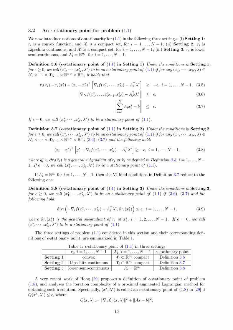
The three settings of problem (1.1) considered in this section and their corresponding defi-nitions of ε-stationary point, are summarized in Table 1.
Table 1: ε-stationary point of (1.1) in three settingsri, i = 1, . . . , N − 1 Xi, i = 1, . . . , N − 1 ε-stationary point
Setting 1 convex Xi ⊂ Rni compact Definition 3.6
Setting 2 Lipschitz continuous Xi ⊂ Rni compact Definition 3.7
Setting 3 lower semi-continuous Xi = Rni Definition 3.8
A very recent work of Hong [29] proposes a definition of ε-stationary point of problem(1.8), and analyzes the iteration complexity of a proximal augmented Lagrangian method forobtaining such a solution. Specifically, (x∗, λ∗) is called an ε-stationary point of (1.8) in [29] ifQ(x∗, λ∗) ≤ ε, where
Q(x, λ) := ‖∇xLβ(x, λ)‖2 + ‖Ax− b‖2,
12
and Lβ(x, λ) := f(x) − λ> (Ax− b) + β2 ‖Ax− b‖
2 is the augmented Lagrangian function of(1.8). Note that [29] assumes that f is differentiable and has bounded gradient in (1.8). Thefollowing result reveals that an ε-stationary point in [29] is equivalent to an O(
√ε)-stationary
point of (1.1) as defined in Definition 3.8 with ri = 0 and f being differentiable. Note thatthere is no set constraint in (1.8), so the definition of ε-stationary point in [29] does not applyto Definitions 3.6 and 3.7.
Proposition 3.9 Consider the ε-stationary point in Definition 3.8 applied to problem (1.8),i.e., one block variable and ri(x) = 0. Then (x∗, λ∗) is a γ1
√ε-stationary point in Definition
3.8, with γ1 = 1/(√
2β2‖A‖22 + 3), implies Q(x∗, λ∗) ≤ ε. On the contrary, if Q(x∗, λ∗) ≤ ε,then (x∗, λ∗) is a γ2
√ε-stationary condition in Definition 3.8, where γ2 =
√2(1 + β2‖A‖22).
Proof. Suppose (x∗, λ∗) is a γ1√ε-stationary point as defined in Definition 3.8. Then we have
‖∇f(x∗)−A>λ∗‖ ≤ γ1
√ε and ‖Ax∗ − b‖ ≤ γ1
√ε,
which implies that
Q(x∗, λ∗) = ‖∇f(x∗)−A>λ∗ + βA>(Ax∗ − b)‖2 + ‖Ax∗ − b‖2
≤ 2‖∇f(x∗)−A>λ∗‖2 + 2β2‖A‖22‖Ax∗ − b‖2 + ‖Ax∗ − b‖2
≤ 2γ21ε+ (2β2‖A‖22 + 1)γ2
1ε = ε.
On the other hand, if Q(x∗, λ∗) ≤ ε, then we have ‖∇f(x∗)−A>λ∗ + βA>(Ax∗ − b)‖2 ≤ ε and‖Ax∗ − b‖2 ≤ ε. Therefore,
‖∇f(x∗)−A>λ∗‖2 ≤ 2‖∇f(x∗)−A>λ∗ + βA>(Ax∗ − b)‖2 + 2‖ − βA>(Ax∗ − b)‖2
≤ 2‖∇f(x∗)−A>λ∗ + βA>(Ax∗ − b)‖2 + 2β2‖A‖22‖Ax∗ − b‖2
≤ 2(1 + β2‖A‖22) ε.
The desired result then follows immediately. �
In the following, we introduce two variants of ADMM, named proximal ADMM-g and prox-imal ADMM-m, that solve (1.1) with some further assumptions on AN . In particular, proximalADMM-g assumes AN = I, and proximal ADMM-m assume AN is full row rank.
3.3 Proximal gradient-based ADMM (proximal ADMM-g)
Our proximal ADMM-g solves (1.1) under the condition that AN = I. Note that when AN = I,the problem is usually referred to as the sharing problem in the literature, and it has a varietyof applications (see, e.g., [12,30,36,37]). Our proximal ADMM-g for solving (1.1) with AN = Iis described in Algorithm 2. It can be seen from Algorithm 2 that proximal ADMM-g is basedon the framework of augmented Lagrangian method, and can be viewed as a variant of theADMM. The augmented Lagrangian function of (1.1) is defined as
Lβ(x1, · · · , xN , λ) := f(x1, · · · , xN ) +N−1∑i=1
ri(xi)−
⟨λ,
N∑i=1
Aixi − b
⟩+β
2
∥∥∥∥∥N∑i=1
Aixi − b
∥∥∥∥∥2
2
,
where λ is the Lagrange multiplier associated with the affine constraint, and β > 0 is a penaltyparameter. In each iteration, proximal ADMM-g minimizes the augmented Lagrangian functionplus a proximal term for block variables x1, . . . , xN−1, with other variables being fixed; and thena gradient descent step was conducted for xN , and finally the Lagrange multiplier λ is updated.
13
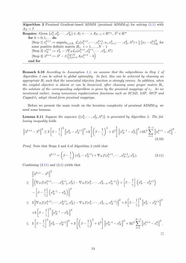
Algorithm 2 Proximal Gradient-based ADMM (proximal ADMM-g) for solving (1.1) withAN = I
Require: Given(x0
1, x02, · · · , x0
N
)∈ X1 × · · · × XN−1 × RnN , λ0 ∈ Rm
for k = 0, 1, . . . do
[Step 1] xk+1i := argminxi∈Xi Lβ(xk+1
1 , · · · , xk+1i−1 , xi, x
ki+1, · · · , xkN , λk)+ 1
2
∥∥xi − xki ∥∥2
Hifor
some positive definite matrix Hi, i = 1, . . . , N − 1[Step 2] xk+1
N := xkN − γ∇NLβ(xk+11 , xk+1
2 , · · · , xkN , λk)[Step 3] λk+1 := λk − β
(∑Ni=1Aix
k+1i − b
)end for
Remark 3.10 According to Assumption 1.1, we assume that the subproblems in Step 1 ofAlgorithm 2 can be solved to global optimality. In fact, this can be achieved by choosing anappropriate Hi such that the associated objective function is strongly convex. In addition, whenthe coupled objective is absent or can be linearized, after choosing some proper matrix Hi,the solution of the corresponding subproblem is given by the proximal mappings of ri. As wementioned earlier, many nonconvex regularization functions such as SCAD, LSP, MCP andCapped-`1 adopt closed-form proximal mappings.
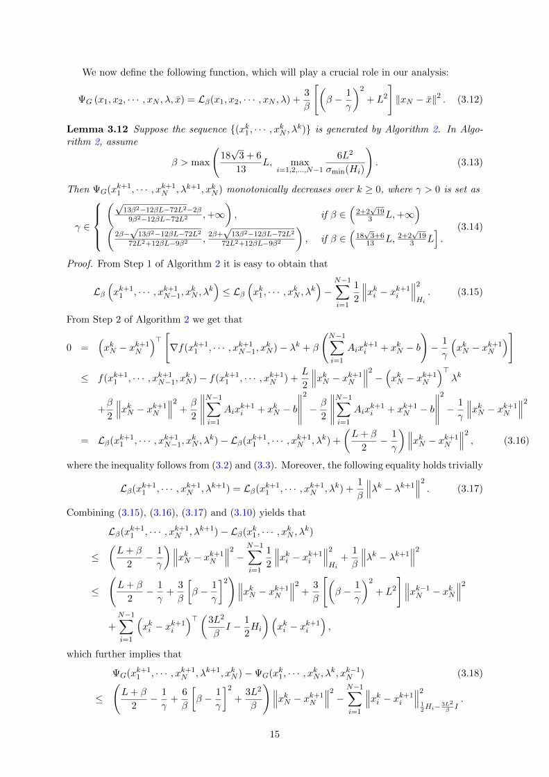
Before we present the main result on the iteration complexity of proximal ADMM-g, weneed some lemmas.
Lemma 3.11 Suppose the sequence {(xk1, · · · , xkN , λk)} is generated by Algorithm 2. The fol-lowing inequality holds
∥∥∥λk+1 − λk∥∥∥2≤ 3
[β − 1
γ
]2 ∥∥∥xkN − xk+1N
∥∥∥2+3
[(β − 1
γ
)2
+ L2
]∥∥∥xk−1N − xkN
∥∥∥2+3L2
N−1∑i=1
∥∥∥xk+1i − xki
∥∥∥2.
(3.10)
Proof. Note that Steps 2 and 3 of Algorithm 2 yield that
λk+1 =
(β − 1
γ
)(xkN − xk+1
N ) +∇Nf(xk+11 , · · · , xk+1
N−1, xkN ). (3.11)
Combining (3.11) and (3.1) yields that∥∥∥λk+1 − λk∥∥∥2
≤∥∥∥∥(∇Nf(xk+1
1 , · · · , xk+1N−1, x
kN )−∇Nf(xk1, · · · , xkN−1, x
k−1N )
)+
[β − 1
γ
](xkN − xk+1
N
)−[β − 1
γ
](xk−1N − xkN
)∥∥∥∥2
≤ 3∥∥∥∇Nf(xk+1
1 , · · · , xk+1N−1, x
kN )−∇Nf(xk1, · · · , xkN−1, x
k−1N )
∥∥∥2+ 3
[β − 1
γ
]2 ∥∥∥xkN − xk+1N
∥∥∥2
+3
[β − 1
γ
]2 ∥∥∥xk−1N − xkN
∥∥∥2
≤ 3
[β − 1
γ
]2 ∥∥∥xkN − xk+1N
∥∥∥2+ 3
[(β − 1
γ
)2
+ L2
]∥∥∥xk−1N − xkN
∥∥∥2+ 3L2
N−1∑i=1
∥∥∥xk+1i − xki
∥∥∥2.
�
14
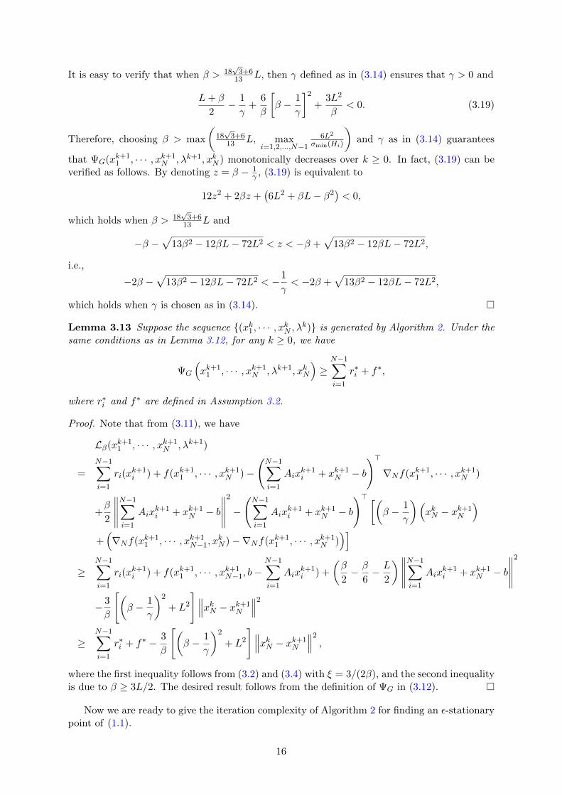
We now define the following function, which will play a crucial role in our analysis:
ΨG (x1, x2, · · · , xN , λ, x) = Lβ(x1, x2, · · · , xN , λ) +3
β
[(β − 1
γ
)2
+ L2
]‖xN − x‖2 . (3.12)
Lemma 3.12 Suppose the sequence {(xk1, · · · , xkN , λk)} is generated by Algorithm 2. In Algo-rithm 2, assume
β > max
(18√
3 + 6
13L, max
i=1,2,...,N−1
6L2
σmin(Hi)
). (3.13)
Then ΨG(xk+11 , · · · , xk+1
N , λk+1, xkN ) monotonically decreases over k ≥ 0, where γ > 0 is set as
γ ∈
(√
13β2−12βL−72L2−2β
9β2−12βL−72L2 ,+∞), if β ∈
(2+2√
193 L,+∞
)(
2β−√
13β2−12βL−72L2
72L2+12βL−9β2 ,2β+√
13β2−12βL−72L2
72L2+12βL−9β2
), if β ∈
(18√
3+613 L, 2+2
√19
3 L].
(3.14)
Proof. From Step 1 of Algorithm 2 it is easy to obtain that
Lβ(xk+1
1 , · · · , xk+1N−1, x
kN , λ
k)≤ Lβ
(xk1, · · · , xkN , λk
)−N−1∑i=1
1
2
∥∥∥xki − xk+1i
∥∥∥2
Hi. (3.15)
From Step 2 of Algorithm 2 we get that
0 =(xkN − xk+1
N
)> [∇f(xk+1
1 , · · · , xk+1N−1, x
kN )− λk + β
(N−1∑i=1
Aixk+1i + xkN − b
)− 1
γ
(xkN − xk+1
N
)]
≤ f(xk+11 , · · · , xk+1
N−1, xkN )− f(xk+1
1 , · · · , xk+1N ) +
L
2
∥∥∥xkN − xk+1N
∥∥∥2−(xkN − xk+1
N
)>λk
+β
2
∥∥∥xkN − xk+1N
∥∥∥2+β
2
∥∥∥∥∥N−1∑i=1
Aixk+1i + xkN − b
∥∥∥∥∥2
− β
2
∥∥∥∥∥N−1∑i=1
Aixk+1i + xk+1
N − b
∥∥∥∥∥2
− 1
γ
∥∥∥xkN − xk+1N
∥∥∥2
= Lβ(xk+11 , · · · , xk+1
N−1, xkN , λ
k)− Lβ(xk+11 , · · · , xk+1
N , λk) +
(L+ β
2− 1
γ
)∥∥∥xkN − xk+1N
∥∥∥2, (3.16)
where the inequality follows from (3.2) and (3.3). Moreover, the following equality holds trivially
Lβ(xk+11 , · · · , xk+1
N , λk+1) = Lβ(xk+11 , · · · , xk+1
N , λk) +1
β
∥∥∥λk − λk+1∥∥∥2. (3.17)
Combining (3.15), (3.16), (3.17) and (3.10) yields that
Lβ(xk+11 , · · · , xk+1
N , λk+1)− Lβ(xk1, · · · , xkN , λk)
≤(L+ β
2− 1
γ
)∥∥∥xkN − xk+1N
∥∥∥2−N−1∑i=1
1
2
∥∥∥xki − xk+1i
∥∥∥2
Hi+
1
β
∥∥∥λk − λk+1∥∥∥2
≤
(L+ β
2− 1
γ+
3
β
[β − 1
γ
]2)∥∥∥xkN − xk+1
N
∥∥∥2+
3
β
[(β − 1
γ
)2
+ L2
]∥∥∥xk−1N − xkN
∥∥∥2
+N−1∑i=1
(xki − xk+1
i
)>(3L2
βI − 1
2Hi
)(xki − xk+1
i
),
which further implies that
ΨG(xk+11 , · · · , xk+1
N , λk+1, xkN )−ΨG(xk1, · · · , xkN , λk, xk−1N ) (3.18)
≤
(L+ β
2− 1
γ+
6
β
[β − 1
γ
]2
+3L2
β
)∥∥∥xkN − xk+1N
∥∥∥2−N−1∑i=1
∥∥∥xki − xk+1i
∥∥∥2
12Hi− 3L2
βI.
15
It is easy to verify that when β > 18√
3+613 L, then γ defined as in (3.14) ensures that γ > 0 and
L+ β
2− 1
γ+
6
β
[β − 1
γ
]2
+3L2
β< 0. (3.19)
Therefore, choosing β > max
(18√
3+613 L, max
i=1,2,...,N−1
6L2
σmin(Hi)
)and γ as in (3.14) guarantees
that ΨG(xk+11 , · · · , xk+1
N , λk+1, xkN ) monotonically decreases over k ≥ 0. In fact, (3.19) can beverified as follows. By denoting z = β − 1
γ , (3.19) is equivalent to
12z2 + 2βz +(6L2 + βL− β2
)< 0,
which holds when β > 18√
3+613 L and
−β −√
13β2 − 12βL− 72L2 < z < −β +√
13β2 − 12βL− 72L2,
i.e.,
−2β −√
13β2 − 12βL− 72L2 < −1
γ< −2β +
√13β2 − 12βL− 72L2,
which holds when γ is chosen as in (3.14). �
Lemma 3.13 Suppose the sequence {(xk1, · · · , xkN , λk)} is generated by Algorithm 2. Under thesame conditions as in Lemma 3.12, for any k ≥ 0, we have
ΨG
(xk+1
1 , · · · , xk+1N , λk+1, xkN
)≥
N−1∑i=1
r∗i + f∗,
where r∗i and f∗ are defined in Assumption 3.2.
Proof. Note that from (3.11), we have
Lβ(xk+11 , · · · , xk+1
N , λk+1)
=
N−1∑i=1
ri(xk+1i ) + f(xk+1
1 , · · · , xk+1N )−
(N−1∑i=1
Aixk+1i + xk+1
N − b
)>∇Nf(xk+1
1 , · · · , xk+1N )
+β
2
∥∥∥∥∥N−1∑i=1
Aixk+1i + xk+1
N − b
∥∥∥∥∥2
−
(N−1∑i=1
Aixk+1i + xk+1
N − b
)> [(β − 1
γ
)(xkN − xk+1
N
)+(∇Nf(xk+1
1 , · · · , xk+1N−1, x
kN )−∇Nf(xk+1
1 , · · · , xk+1N )
)]≥
N−1∑i=1
ri(xk+1i ) + f(xk+1
1 , · · · , xk+1N−1, b−
N−1∑i=1
Aixk+1i ) +
(β
2− β
6− L
2
)∥∥∥∥∥N−1∑i=1
Aixk+1i + xk+1
N − b
∥∥∥∥∥2
− 3
β
[(β − 1
γ
)2
+ L2
]∥∥∥xkN − xk+1N
∥∥∥2
≥N−1∑i=1
r∗i + f∗ − 3
β
[(β − 1
γ
)2
+ L2
]∥∥∥xkN − xk+1N
∥∥∥2,
where the first inequality follows from (3.2) and (3.4) with ξ = 3/(2β), and the second inequalityis due to β ≥ 3L/2. The desired result follows from the definition of ΨG in (3.12). �
Now we are ready to give the iteration complexity of Algorithm 2 for finding an ε-stationarypoint of (1.1).
16
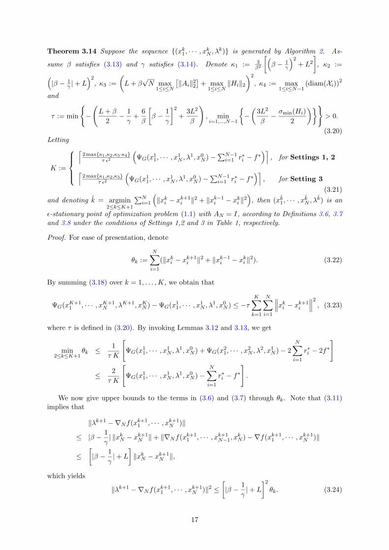
Theorem 3.14 Suppose the sequence {(xk1, · · · , xkN , λk)} is generated by Algorithm 2. As-
sume β satisfies (3.13) and γ satisfies (3.14). Denote κ1 := 3β2
[(β − 1
γ
)2+ L2
], κ2 :=(
|β − 1γ |+ L
)2, κ3 :=
(L+ β
√N max
1≤i≤N
[‖Ai‖22
]+ max
1≤i≤N‖Hi‖2
)2
, κ4 := max1≤i≤N−1
(diam(Xi))2
and
τ := min
{−
(L+ β
2− 1
γ+
6
β
[β − 1
γ
]2
+3L2
β
), mini=1,...,N−1
{−(
3L2
β− σmin(Hi)
2
)}}> 0.
(3.20)Letting
K :=
⌈
2 max{κ1,κ2,κ3·κ4}τ ε2
(ΨG(x1
1, · · · , x1N , λ
1, x0N )−
∑N−1i=1 r∗i − f∗
)⌉, for Settings 1, 2
⌈2 max{κ1,κ2,κ3}
τ ε2
(ΨG(x1
1, · · · , x1N , λ
1, x0N )−
∑N−1i=1 r∗i − f∗
)⌉, for Setting 3
(3.21)
and denoting k = argmin2≤k≤K+1
∑Ni=1
(‖xki − x
k+1i ‖2 + ‖xk−1
i − xki ‖2)
, then (xk1, · · · , xkN , λk) is an
ε-stationary point of optimization problem (1.1) with AN = I, according to Definitions 3.6, 3.7and 3.8 under the conditions of Settings 1,2 and 3 in Table 1, respectively.
Proof. For ease of presentation, denote
θk :=
N∑i=1
(‖xki − xk+1i ‖2 + ‖xk−1
i − xki ‖2). (3.22)
By summing (3.18) over k = 1, . . . ,K, we obtain that
ΨG(xK+11 , · · · , xK+1
N , λK+1, xKN )−ΨG(x11, · · · , x1
N , λ1, x0
N ) ≤ −τK∑k=1
N∑i=1
∥∥∥xki − xk+1i
∥∥∥2, (3.23)
where τ is defined in (3.20). By invoking Lemmas 3.12 and 3.13, we get
min2≤k≤K+1
θk ≤ 1
τ K
[ΨG(x1
1, · · · , x1N , λ
1, x0N ) + ΨG(x2
1, · · · , x2N , λ
2, x1N )− 2
N∑i=1
r∗i − 2f∗
]
≤ 2
τ K
[ΨG(x1
1, · · · , x1N , λ
1, x0N )−
N∑i=1
r∗i − f∗].
We now give upper bounds to the terms in (3.6) and (3.7) through θk. Note that (3.11)implies that
‖λk+1 −∇Nf(xk+11 , · · · , xk+1
N )‖
≤ |β − 1
γ| ‖xkN − xk+1
N ‖+ ‖∇Nf(xk+11 , · · · , xk+1
N−1, xkN )−∇f(xk+1
1 , · · · , xk+1N )‖
≤[|β − 1
γ|+ L
]‖xkN − xk+1
N ‖,
which yields
‖λk+1 −∇Nf(xk+11 , · · · , xk+1
N )‖2 ≤[|β − 1
γ|+ L
]2
θk. (3.24)
17
From Step 3 of Algorithm 2 and (3.10) it is easy to see that∥∥∥∥∥N−1∑i=1
Aixk+1i + xk+1
N − b
∥∥∥∥∥2
=1
β2‖λk+1 − λk‖2
≤ 3
β2
[β − 1
γ
]2 ∥∥∥xkN − xk+1N
∥∥∥2+
3
β2
[(β − 1
γ
)2
+ L2
]∥∥∥xk−1N − xkN
∥∥∥2+
3L2
β2
N−1∑i=1
∥∥∥xki − xk+1i
∥∥∥2
≤ 3
β2
[(β − 1
γ
)2
+ L2
]θk. (3.25)
We now give upper bounds to the terms in (3.5), (3.8) and (3.9) under the three settings inTable 1, respectively.
Setting 3. Because ri is lower semi-continuous and Xi = Rni , i = 1, . . . , N − 1, it followsfrom Step 1 of Algorithm 2 that there exists a general subgradient gi ∈ ∂ri(xk+1
i ) such that
dist(−∇if(xk+1
1 , · · · , xk+1N ) +A>i λ
k+1, ∂ri(xk+1i )
)(3.26)
≤∥∥∥gi +∇if(xk+1
1 , · · · , xk+1N )−A>i λk+1
∥∥∥=
∥∥∥∥∇if(xk+11 , · · · , xk+1
N )−∇if(xk+11 , · · · , xk+1
i , xki+1, · · · , xkN )
+βA>i
( N∑j=i+1
Aj(xk+1j − xkj )
)−Hi(x
k+1i − xki )
∥∥∥∥≤ L
√√√√ N∑j=i+1
‖xkj − xk+1j ‖2 + β ‖Ai‖2
N∑j=i+1
‖Aj‖2‖xk+1j − xkj ‖+ ‖Hi‖2‖xk+1
i − xki ‖2
≤(L+ β
√N max
i+1≤j≤N[‖Aj‖2] ‖Ai‖2
) √√√√ N∑j=i+1
‖xkj − xk+1j ‖2 + ‖Hi‖2‖xk+1
i − xki ‖2
≤(L+ β
√N max
1≤i≤N
[‖Ai‖22
]+ max
1≤i≤N‖Hi‖2
)√θk.
By combining (3.26), (3.24) and (3.25) we conclude that Algorithm 2 returns an ε-stationarypoint of (1.1) according to Definition 3.8 under conditions in Setting 3 in Table 1.
Setting 2. Under this setting, we know ri is Lipschitz continuous and Xi ⊂ Rni is convexand compact. Because f(x1, · · · , xN ) is differentiable, we know ri(xi) + f(x1, · · · , xN ) is locallyLipschitz continuous with respect to xi for i = 1, 2, . . . , N−1. Similar to (3.26), for any xi ∈ Xi,Step 1 of Algorithm 2 yields that(
xi − xk+1i
)> [gi +∇if(xk+1
1 , · · · , xk+1N )−A>i λk+1
](3.27)
≥(xi − xk+1
i
)> [∇if(xk+1
1 , · · · , xk+1N )−∇if(xk+1
1 , · · · , xk+1i , xki+1, · · · , xkN )
+βA>i
( N∑j=i+1
Aj(xk+1j − xkj )
)−Hi(x
k+1i − xki )
]
≥ −Ldiam(Xi)
√√√√ N∑j=i+1
‖xkj − xk+1j ‖2 − β‖Ai‖2 diam(Xi)
N∑j=i+1
‖Aj‖2‖xk+1j − xkj ‖
−diam(Xi) ‖Hi‖2‖xk+1i − xki ‖2
≥ −(β√N max
1≤i≤N
[‖Ai‖22
]+ L+ max
1≤i≤N‖Hi‖2
)max
1≤i≤N−1[diam(Xi)]
√θk,
18
where gi ∈ ∂ri(xk+1i ) is a general subgradient of ri at xk+1
i . By combining (3.27), (3.24)and (3.25) we conclude that Algorithm 2 returns an ε-stationary point of (1.1) according toDefinition 3.7 under conditions in Setting 2 in Table 1.
Setting 1. Under this setting, ri is convex, so gi in (3.27) becomes a subgradient of ri atxk+1i . Therefore, for i = 1, 2, · · · , N − 1 and any xi ∈ Xi we have that
ri(xi)− ri(xk+1i ) +
(xi − xk+1
i
)> [∇if(xk+1
1 , · · · , xk+1N )−A>i λk+1
](3.28)
≥(xi − xk+1
i
)> [gi +∇if(xk+1
1 , · · · , xk+1N )−A>i λk+1
]≥ −
(β√N max
1≤i≤N
[‖Ai‖22
]+ L+ max
1≤i≤N‖Hi‖2
)max
1≤i≤N−1[diam(Xi)]
√θk.
By combining (3.28), (3.24) and (3.25) we conclude that Algorithm 2 returns an ε-stationarypoint of (1.1) according to Definition 3.6 under the conditions of Setting 1 in Table 1. �
Remark 3.15 Note that the potential function ΨG defined in (3.12) is related to the augmentedLagrangian function. The augmented Lagrangian function has been used as a potential functionin analyzing the convergence of nonconvex splitting and ADMM methods in [2, 28–30, 35]. See[29] for a more detailed discussion on this.
Remark 3.16 In Step 1 of Algorithm 2, we can also replace the function
f(xk+11 , · · · , xk+1
i−1 , xi, xki+1, · · · , xkN )
by its linearization
f(xk+11 , · · · , xk+1
i−1 , xki , x
ki+1, · · · , xkN ) +
(xi − xki
)>∇if(xk+1
1 , · · · , xk+1i−1 , x
ki , x
ki+1, · · · , xN ),
so that the subproblem can be solved by computing the proximal mappings of ri, with someproperly chosen matrix Hi. Under the additional condition that∥∥∇if(x1
1, x12, · · · , x1
N )−∇if(x21, x
22, · · · , x2
N )∥∥ ≤ Li ∥∥(x1
1 − x21, x
12 − x2
2, · · · , x1N − x2
N
)∥∥ .and setting Hi � LiI for i = 1, . . . , N − 1, the same iteration bound still holds by slightlymodifying the analysis above.
3.4 Proximal majorization ADMM (proximal ADMM-m)
Our proximal ADMM-m solves (1.1) under the condition that AN is full row rank. In thissection, we use σN to denote the smallest eigenvalue of ANA
>N . Note that σN > 0 because
AN is full row rank. Our proximal ADMM-m can be described as in Algorithm 3, whereU(x1, · · · , xN−1, xN , λ, x) is defined as
U(x1, · · · , xN−1, xN , λ, x) = f(x1, · · · , xN−1, x) + (xN − x)>∇Nf(x1, · · · , xN−1, x)
+L
2‖xN − x‖2 −
⟨λ,
N∑i=1
Aixi − b
⟩+β
2
∥∥∥∥∥N∑i=1
Aixi − b
∥∥∥∥∥2
.
It is worth noting the proximal ADMM-m and proximal ADMM-g differ only in Step 2:Step 2 of proximal ADMM-g takes a gradient step of the augmented Lagrangian function withrespect to xN , while Step 2 of proximal ADMM-m requires to minimize a quadratic function ofxN .
We provide some lemmas that are useful in analyzing the iteration complexity of proximalADMM-m for solving (1.1).
19
Algorithm 3 Proximal majorization ADMM (proximal ADMM-m) for solving (1.1) with ANbeing full row rank
Require: Given(x0
1, x02, · · · , x0
N
)∈ X1 × · · · × XN−1 × RnN , λ0 ∈ Rm
for k = 0, 1, . . . do
[Step 1] xk+1i := argminxi∈Xi Lβ(xk+1
1 , · · · , xk+1i−1 , xi, x
ki+1, · · · , xkN , λk)+ 1
2
∥∥xi − xki ∥∥2
Hifor
some positive definite matrix Hi, i = 1, . . . , N − 1[Step 2] xk+1
N := argminxN U(xk+11 , · · · , xk+1
N−1, xN , λk, xkN )
[Step 3] λk+1 := λk − β(∑N
i=1Aixk+1i − b
)end for
Lemma 3.17 Suppose the sequence {(xk1, · · · , xkN , λk)} is generated by Algorithm 3. The fol-lowing inequality holds∥∥∥λk+1 − λk
∥∥∥2≤ 3L2
σN
∥∥∥xkN − xk+1N
∥∥∥2+
6L2
σN
∥∥∥xk−1N − xkN
∥∥∥2+
3L2
σN
N−1∑i=1
∥∥∥xki − xk+1i
∥∥∥2. (3.29)
Proof. From the optimality conditions of Step 2 of Algorithm 3, we have
0 = ∇Nf(xk+11 , · · · , xk+1
N−1, xkN )−A>Nλk + βA>N
(N∑i=1
Aixk+1i − b
)− L
(xkN − xk+1
N
)= ∇Nf(xk+1
1 , · · · , xk+1N−1, x
kN )−A>Nλk+1 − L
(xkN − xk+1
N
),
where the second equality is due to Step 3 of Algorithm 3. Therefore, we have
‖λk+1 − λk‖2 ≤ σ−1N ‖A
>Nλ
k+1 −A>Nλk‖2
≤ σ−1N ‖(∇Nf(xk+1
1 , · · · , xk+1N−1, x
kN )−∇Nf(xk1, · · · , xkN−1, x
k−1N ))− L(xkN − xk+1
N ) + L(xk−1N − xkN )‖2
≤ 3
σN‖∇Nf(xk+1
1 , · · · , xk+1N−1, x
kN )−∇Nf(xk1, · · · , xkN−1, x
k−1N )‖2 +
3L2
σN(‖xkN − xk+1
N ‖2 + ‖xk−1N − xkN‖2)
≤ 3L2
σN‖xkN − xk+1
N ‖2 +6L2
σN‖xk−1
N − xkN‖2 +3L2
σN
N−1∑i=1
‖xki − xk+1i ‖2.
�
We define the following function that will be used in the analysis of proximal ADMM-m:
ΨL (x1, · · · , xN , λ, x) = Lβ(x1, · · · , xN , λ) +6L2
βσN‖xN − x‖2 .
Similar as the function used in proximal ADMM-g, we can prove the monotonicity and bound-edness of function ΨL.
Lemma 3.18 Suppose the sequence {(xk1, · · · , xkN , λk)} is generated by Algorithm 3. In Algo-rithm 3, assume
β > max
{18L
σN, max
1≤i≤N−1
{6L2
σNσmin(Hi)
}}. (3.30)
Then ΨL(xk+1, · · · , xk+1N , λk+1, xkN ) monotonically decreases over k > 0.
Proof. By Step 1 of Algorithm 3 one observes that
Lβ(xk+1
1 , · · · , xk+1N−1, x
kN , λ
k)≤ Lβ
(xk1, · · · , xkN , λk
)−N−1∑i=1
1
2
∥∥∥xki − xk+1i
∥∥∥2
Hi, (3.31)
20
while by Step 2 of Algorithm 3 we have
0 =(xkN − xk+1
N
)> [∇Nf(xk+1
1 , · · · , xk+1N−1, x
kN )−AN>λk + βAN
>
(N∑i=1
Aixk+1i − b
)− L
(xkN − xk+1
N
)]
≤ f(xk+11 , · · · , xk+1
N−1, xkN )− f(xk+1
1 , · · · , xk+1N )− L
2
∥∥∥xkN − xk+1N
∥∥∥2−
(N−1∑i=1
Aixk+1i +ANx
kN − b
)>λk
+
(N∑i=1
Aixk+1i − b
)>λk +
β
2
∥∥∥∥∥N−1∑i=1
Aixk+1i +ANx
kN − b
∥∥∥∥∥2
− β
2
∥∥∥∥∥N∑i=1
Aixk+1i − b
∥∥∥∥∥2
−β2
∥∥∥ANxkN −ANxk+1N
∥∥∥2
≤ Lβ(xk+11 , · · · , xk+1
N−1, xkN , λ
k)− Lβ(xk+11 , · · · , xk+1
N , λk)− L
2
∥∥∥xkN − xk+1N
∥∥∥2, (3.32)
where the first inequality is due to (3.2) and (3.3). Moreover, from (3.29) we have
Lβ(xk+11 , · · · , xk+1
N , λk+1)− Lβ(xk+11 , · · · , xk+1
N , λk) =1
β‖λk − λk+1‖2
≤ 3L2
βσN‖xkN − xk+1
N ‖2 +6L2
βσN‖xk−1
N − xkN‖2 +3L2
βσN
N−1∑i=1
‖xki − xk+1i ‖2. (3.33)
Combining (3.31), (3.32) and (3.33) yields that
Lβ(xk+11 , · · · , xk+1
N , λk+1)− Lβ(xk1, · · · , xkN , λk)
≤(
3L2
βσN− L
2
)‖xkN − xk+1
N ‖2 +
N−1∑i=1
‖xki − xk+1i ‖23L2
βσNI− 1
2Hi
+6L2
βσN‖xk−1
N − xkN‖2,
which further implies that
ΨL(xk+11 , · · · , xk+1
N , λk+1, xkN )−ΨL(xk1, · · · , xkN , λk, xk−1N ) (3.34)
≤(
9L2
βσN− L
2
)∥∥∥xkN − xk+1N
∥∥∥2+
N−1∑i=1
(3L2
βσN− σmin(Hi)
2
)∥∥∥xki − xk+1i
∥∥∥2< 0,
where the second inequality is due to (3.30). This completes the proof. �
The following lemma shows that the function ΨL is lower bounded.
Lemma 3.19 Suppose the sequence {(xk1, · · · , xkN , λk)} is generated by Algorithm 3. Under thesame conditions as in Lemma 3.18, the sequence {ΨL(xk+1, · · · , xk+1
N , λk+1, xkN )} is boundedfrom below.
Proof. From Step 3 of Algorithm 3 we have
ΨL(xk+11 , · · · , xk+1
N , λk+1, xkN ) ≥ Lβ(xk+11 , · · · , xk+1
N , λk+1)
=N−1∑i=1
ri(xk+1i ) + f(xk+1
1 , · · · , xk+1N )−
(N∑i=1
Aixk+1i − b
)>λk+1 +
β
2
∥∥∥∥∥N∑i=1
Aixk+1i − b
∥∥∥∥∥2
(3.35)
=N−1∑i=1
ri(xk+1i ) + f(xk+1
1 , · · · , xk+1N )− 1
β(λk − λk+1)>λk+1 +
1
2β‖λk − λk+1‖2
=
N−1∑i=1
ri(xk+1i ) + f(xk+1
1 , · · · , xk+1N )− 1
2β‖λk‖2 +
1
2β‖λk+1‖2 +
1
β‖λk − λk+1‖2
≥N−1∑i=1
r∗i + f∗ − 1
2β‖λk‖2 +
1
2β‖λk+1‖2,
21
where the third equality follows from (3.3). Summing this inequality over k = 0, 1, . . . ,K − 1for any integer K ≥ 1 yields that
1
K
K−1∑k=0
ΨL
(xk+1
1 , · · · , xk+1N , λk+1, xkN
)≥
N−1∑i=1
r∗i + f∗ − 1
2β
∥∥λ0∥∥2.
Lemma 3.18 stipulates that {ΨL(xk+11 , . . . , xk+1
N , λk+1, xkN )} is a monotonically decreasing se-quence; the above inequality thus further implies that the entire sequence is bounded frombelow. �
We are now ready to give the iteration complexity of proximal ADMM-m, whose proof issimilar to that of Theorem 3.14.
Theorem 3.20 Suppose the sequence {(xk1, · · · , xkN , λk)} is generated by proximal ADMM-m(Algorithm 3), and β satisfies (3.30). Denote
κ1 :=6L2
β2σN, κ2 := 4L2, κ3 :=
(L+ β
√N max
1≤i≤N
[‖Ai‖22
]+ max
1≤i≤N‖Hi‖2
)2
, κ4 := max1≤i≤N−1
(diam(Xi))2
and
τ := min
{−(
9L2
βσN− L
2
), mini=1,...,N−1
{−(
3L2
βσN− σmin(Hi)
2
)}}> 0. (3.36)
Letting
K :=
⌈
2 max{κ1,κ2,κ3·κ4}τ ε2
(ΨL(x11, · · · , x1
N , λ1, x0
N )−∑N−1
i=1 r∗i − f∗)⌉, for Settings 1,2
⌈2 max{κ1,κ2,κ3}
τ ε2(ΨL(x1
1, · · · , x1N , λ
1, x0N )−
∑N−1i=1 r∗i − f∗)
⌉, for Setting 3
(3.37)
and denoting k := min2≤k≤K+1
∑Ni=1
(‖xki − x
k+1i ‖2 + ‖xk−1
i − xki ‖2)
, then (xk1, · · · , xkN , λk) is an
ε-stationary point of problem (1.1) with AN being full row rank, according to Definitions 3.6,3.7 and 3.8 under the conditions of Settings 1,2 and 3 in Table 1, respectively.
Proof. By summing (3.34) over k = 1, . . . ,K, we obtain that
ΨL(xK+11 , · · · , xK+1
N , λK+1, xKN )−ΨL(x11, · · · , x1
N , λ1, x0
N ) ≤ −τK∑k=1
N∑i=1
∥∥∥xki − xk+1i
∥∥∥2, (3.38)
where τ is defined in (3.36). From Lemma 3.19 we know that there exists a constant Ψ∗L suchthat Ψ(xk+1
1 , · · · , xk+1N , λk+1, xkN ) ≥ Ψ∗L holds for any k ≥ 1. Therefore,
min2≤k≤K+1
θk ≤2
τ K
[ΨL(x1
1, · · · , x1N , λ
1, x0N )−Ψ∗L
], (3.39)
where θk is defined in (3.22), i.e., for K defined as in (3.37), θk = O(ε2).We now give upper bounds to the terms in (3.6) and (3.7) through θk. Note that (3.30)
implies that
‖A>Nλk+1 −∇Nf(xk+11 , · · · , xk+1
N )‖≤ L ‖xkN − xk+1
N ‖+ ‖∇Nf(xk+11 , · · · , xk+1
N−1, xkN )−∇Nf(xk+1
1 , · · · , xk+1N )‖
≤ 2L ‖xkN − xk+1N ‖,
which implies that‖A>Nλk+1 −∇Nf(xk+1
1 , · · · , xk+1N )‖2 ≤ 4L2θk. (3.40)
22
By Step 3 of Algorithm 3 and (3.29) we have∥∥∥∥∥N∑i=1
Aixk+1i − b
∥∥∥∥∥2
=1
β2‖λk+1 − λk‖2 (3.41)
≤ 3L2
β2σN
∥∥∥xkN − xk+1N
∥∥∥2+
6L2
β2σN
∥∥∥xk−1N − xkN
∥∥∥2+
3L2
β2σN
N−1∑i=1
∥∥∥xki − xk+1i
∥∥∥2≤ 6L2
β2σNθk.
The remaining proof is to give upper bounds to the terms in (3.5), (3.8) and (3.9). Sincethe proof steps are very similar to the that of Theorem 3.14, we shall only provide the keyinequalities below.
Setting 3. Under conditions in Setting 3 in Table 1, the inequality (3.26) becomes
dist(−∇if(xk+1
1 , · · · , xk+1N ) +A>i λ
k+1, ∂ri(xk+1i )
)≤
(L+ β
√N max
1≤i≤N
[‖Ai‖22
]+ max
1≤i≤N‖Hi‖2
)√θk. (3.42)
By combining (3.42), (3.40) and (3.41) we conclude that Algorithm 3 returns an ε-stationarypoint of (1.1) according to Definition 3.8 under conditions in Setting 3 in Table 1.
Setting 2. Under conditions in Setting 2 in Table 1, the inequality (3.27) becomes(xi − xk+1
i
)> [gi +∇if(xk+1
1 , · · · , xk+1N )−A>i λk+1
]≥ −
(β√N max
1≤i≤N
[‖Ai‖22
]+ L+ max
1≤i≤N‖Hi‖2
)max
1≤i≤N−1[diam(Xi)]
√θk. (3.43)
By combining (3.43), (3.40) and (3.41) we conclude that Algorithm 3 returns an ε-stationarypoint of (1.1) according to Definition 3.7 under conditions in Setting 2 in Table 1.
Setting 1. Under conditions in Setting 1 in Table 1, inequality (3.28) becomes
ri(xi)− ri(xk+1i ) +
(xi − xk+1
i
)> [∇if(xk+1
1 , · · · , xk+1N )−A>i λk+1
]≥ −
(β√N max
1≤i≤N
[‖Ai‖22
]+ L+ max
1≤i≤N‖Hi‖2
)max
1≤i≤N−1[diam(Xi)]
√θk. (3.44)
By combining (3.44), (3.40) and (3.41) we conclude that Algorithm 3 returns an ε-stationarypoint of (1.1) according to Definition 3.6 under conditions in Setting 1 in Table 1. �
Remark 3.21 In Step 1 of Algorithm 3, we can replace the function f(xk+11 , · · · , xk+1
i−1 , xi, xki+1, · · · , xkN )
by its linearization
f(xk+11 , · · · , xk+1
i−1 , xki , x
ki+1, · · · , xkN ) +
(xi − xki
)>∇if(xk+1
1 , · · · , xk+1i−1 , x
ki , x
ki+1, · · · , xN ).
Under the same conditions as in Remark 3.16, the same iteration bound follows by slightlymodifying the analysis above.
4 Extensions
4.1 Relax the assumption on the last block variable xN
It is noted that in (1.1), we have some restrictions on the last block variable xN , i.e., rN ≡ 0,XN = RnN and AN = I or is full row rank. A more general problem to consider is
min f(x1, x2, · · · , xN ) +N∑i=1
ri(xi)
s.t.∑N
i=1Aixi = b, xi ∈ Xi, i = 1, . . . , N,
(4.1)
23
with the same assumptions as in (1.1), plus XN ⊂ RnN being a compact set. Note that we do notassume AN = I nor that AN is full row rank. Moreover, note that if rN = 0 and XN = RnN ,then (4.1) reduces to (1.1). In the following, we shall briefly illustrate how to use proximalADMM-m to find an ε-stationary point of (4.1), and proximal ADMM-g can be applied in thesame manner. We introduce the following problem that is closely related to (4.1):
min f(x1, x2, · · · , xN ) +N∑i=1
ri(xi) + µ2‖xN+1‖2
s.t.∑N
i=1Aixi + xN+1 = b, xi ∈ Xi, i = 1, . . . , N,
(4.2)
where µ > 0. Now proximal ADMM-m is ready to be used for solving (4.2) because AN+1 = Iand xN+1 is unconstrained. We have the following iteration complexity result for proximalADMM-m to obtain an ε-stationary point of (4.1).
Theorem 4.1 Suppose the sequence {(xk1, · · · , xkN+1, λk)} is generated by proximal ADMM-m
for solving (4.2) with µ = 1/ε2, where ε > 0 is the given tolerance. Under the same conditions
and using the same notation as in Theorem 3.20, (xk1, · · · , xkN+1, λk) is an ε-stationary point of
(4.2), and (xk1, · · · , xkN , λk) is an ε-stationary point of (4.1), according to Definitions 3.6, 3.7and 3.8 under conditions in Settings 1,2 and 3 in Table 1, respectively.
Proof. We only show the case for Setting 3 in Table 1, i.e., Definition 3.8, and the other twosettings can be proved similarly. Note that if (x∗1, · · · , x∗N+1, λ
∗) satisfies (3.9), (3.6) and (3.7)with N being replaced by N + 1, then it is an ε-stationary point of (4.2). Therefore, accordingto Theorem 3.20, we have
dist(−∇if(xk1, · · · , xkN ) +A>i λ
k, ∂ri(xki ))≤ ε, for i = 1, . . . , N, (4.3)∥∥∥∥∥
N∑i=1
Aixki + xkN+1 − b
∥∥∥∥∥ ≤ ε. (4.4)
From (3.35), it holds that
ΨL(xk+11 , · · · , xk+1
N+1, λk+1, xkN+1)
≥N∑i=1
ri(xk+1i ) + f(xk+1
1 , · · · , xk+1N ) +
‖xk+1N+1‖2
2ε2−
(N+1∑i=1
Aixk+1i − b
)>λk+1 +
β
2
∥∥∥∥∥N+1∑i=1
Aixk+1i − b
∥∥∥∥∥2
≥N∑i=1
r∗i + f∗ +‖xk+1
N+1‖2
2ε2− 1
2β‖λk+1‖2 − β
2
∥∥∥∥∥N+1∑i=1
Aixk+1i − b
∥∥∥∥∥2
+β
2
∥∥∥∥∥N+1∑i=1
Aixk+1i − b
∥∥∥∥∥2
.
Moreover, by Step 2 of Algorithm 3, we have that xk+1N+1 = ε2λk+1 in this particular problem.
Recall that in Theorem 3.20, β ≥ 18L = 18µ = 18/ε2. Therefore, when β > 1ε2
, the above in-
equality combined with monotonically decreasing of {ΨL(xk+11 , · · · , xk+1
N+1, λk+1, xkN+1)} implies
that
17
18
‖xk+1N+1‖2
2ε2≤ (1− 1/(βε2))
‖xk+1N+1‖2
2ε2≤ ΨL(x1
1, · · · , x1N+1, λ
1, x0N+1)−
N∑i=1
r∗i − f∗
As a result, the sequence
{‖xk+1N+1‖
2
2ε2
}is bounded. Therefore, from (4.4) we get∥∥∥∥∥
N∑i=1
Aixki − b
∥∥∥∥∥ ≤∥∥∥∥∥N∑i=1
Aixki + xkN+1 − b
∥∥∥∥∥+∥∥∥xkN+1
∥∥∥ ≤ Cε, (4.5)
for some constant C > 0. Finally, (4.3) and (4.5) imply that (xk1, · · · , xkN , λk) is an ε-stationarypoint of (4.1), according to Definition 3.8 under the conditions of Setting 3 in Table 1. �
24
4.2 Proximal BCD (Block Coordinate Descent)
In this section, we propose a proximal block coordinate descent method for solving the followingvariant of (1.1) and prove its iteration complexity:
min F (x1, x2, · · · , xN ) := f(x1, x2, · · · , xN ) +N∑i=1
ri(xi)
s.t. xi ∈ Xi, i = 1, . . . , N,
(4.6)
where f is differentiable, ri is nonsmooth, and Xi ⊂ Rni is a closed convex set for i = 1, 2, . . . , N .Note that f and ri can be nonconvex functions. Our proximal BCD method for solving (4.6) isdescribed in Algorithm 4.
Algorithm 4 A proximal BCD method for solving (4.6)
Require: Given(x0
1, x02, · · · , x0
N
)∈ X1 × · · · × XN
for k = 0, 1, . . . doUpdate block xi in a cyclic order, i.e., for i = 1, . . . , N (Hi positive definite):
xk+1i := argmin
xi∈XiF (xk+1
1 , · · · , xk+1i−1 , xi, x
ki+1, · · · , xkN ) +
1
2
∥∥∥xi − xki ∥∥∥2
Hi. (4.7)
end for
Similar as settings in Table 1, depending on the properties of ri and Xi, the ε-stationarypoint of (4.6) can be defined as follows.
Definition 4.2 (x∗1, . . . , x∗N , λ
∗) is called an ε-stationary point of (4.6), if
(i) ri is convex, Xi is convex and compact, and for any xi ∈ Xi, i = 1, . . . , N , it holds that
ri(xi)− ri(x∗i ) + (xi − x∗i )>[∇if(x∗1, · · · , x∗N )−A>i λ∗
]≥ −ε;
(ii) or, if ri is Lipschitz continuous, Xi is convex and compact, and for any xi ∈ Xi, i =1, . . . , N , it holds that (gi = ∂ri(x
∗i ) denotes a generalized subgradient of ri)
(xi − x∗i )>[∇if(x∗1, · · · , x∗N ) + gi −A>i λ∗
]≥ −ε;
(iii) or, if ri is lower semi-continuous, Xi = Rni for i = 1, . . . , N , it holds that
dist(−∇if(x∗1, · · · , x∗N ) +A>i λ
∗, ∂ri(x∗i ))≤ ε.
We now show that the iteration complexity of Algorithm 4 can be obtained from that ofproximal ADMM-g. By introducing an auxiliary variable xN+1 and an arbitrary vector b ∈ Rm,problem (4.6) can be equivalently rewritten as
min f(x1, x2, · · · , xN ) +N∑i=1
ri(xi)
s.t. xN+1 = b, xi ∈ Xi, i = 1, . . . , N.
(4.8)
It is easy to see that applying proximal ADMM-g to solve (4.8) (with xN+1 being the last blockvariable) reduces exactly to Algorithm 4. Hence, we have the following iteration complexityresult of Algorithm 4 for obtaining an ε-stationary point of (4.6).
25
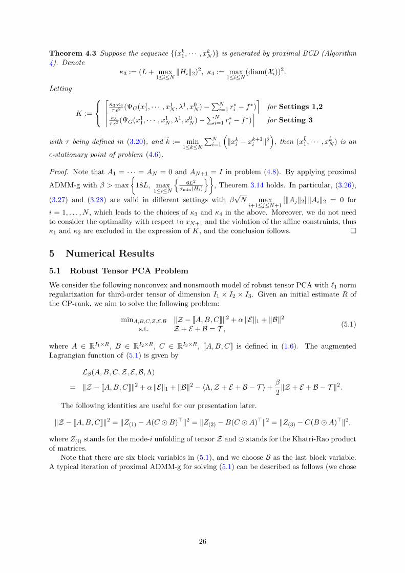
Theorem 4.3 Suppose the sequence {(xk1, · · · , xkN )} is generated by proximal BCD (Algorithm4). Denote
κ3 := (L+ max1≤i≤N
‖Hi‖2)2, κ4 := max1≤i≤N
(diam(Xi))2.
Letting
K :=
⌈κ3·κ4τ ε2
(ΨG(x11, · · · , x1
N , λ1, x0
N )−∑N
i=1 r∗i − f∗)
⌉for Settings 1,2⌈
κ3τ ε2
(ΨG(x11, · · · , x1
N , λ1, x0
N )−∑N
i=1 r∗i − f∗)
⌉for Setting 3
with τ being defined in (3.20), and k := min1≤k≤K
∑Ni=1
(‖xki − x
k+1i ‖2
), then (xk1, · · · , xkN ) is an
ε-stationary point of problem (4.6).
Proof. Note that A1 = · · · = AN = 0 and AN+1 = I in problem (4.8). By applying proximal
ADMM-g with β > max
{18L, max
1≤i≤N
{6L2
σmin(Hi)
}}, Theorem 3.14 holds. In particular, (3.26),
(3.27) and (3.28) are valid in different settings with β√N max
i+1≤j≤N+1[‖Aj‖2] ‖Ai‖2 = 0 for
i = 1, . . . , N , which leads to the choices of κ3 and κ4 in the above. Moreover, we do not needto consider the optimality with respect to xN+1 and the violation of the affine constraints, thusκ1 and κ2 are excluded in the expression of K, and the conclusion follows. �
5 Numerical Results
5.1 Robust Tensor PCA Problem
We consider the following nonconvex and nonsmooth model of robust tensor PCA with `1 normregularization for third-order tensor of dimension I1 × I2 × I3. Given an initial estimate R ofthe CP-rank, we aim to solve the following problem:
minA,B,C,Z,E,B ‖Z − JA,B,CK‖2 + α ‖E‖1 + ‖B‖2s.t. Z + E + B = T , (5.1)
where A ∈ RI1×R, B ∈ RI2×R, C ∈ RI3×R, JA,B,CK is defined in (1.6). The augmentedLagrangian function of (5.1) is given by
Lβ(A,B,C,Z, E ,B,Λ)
= ‖Z − JA,B,CK‖2 + α ‖E‖1 + ‖B‖2 − 〈Λ,Z + E + B − T 〉+β
2‖Z + E + B − T ‖2.
The following identities are useful for our presentation later.
‖Z − JA,B,CK‖2 = ‖Z(1) −A(C �B)>‖2 = ‖Z(2) −B(C �A)>‖2 = ‖Z(3) − C(B �A)>‖2,
where Z(i) stands for the mode-i unfolding of tensor Z and � stands for the Khatri-Rao productof matrices.
Note that there are six block variables in (5.1), and we choose B as the last block variable.A typical iteration of proximal ADMM-g for solving (5.1) can be described as follows (we chose
26
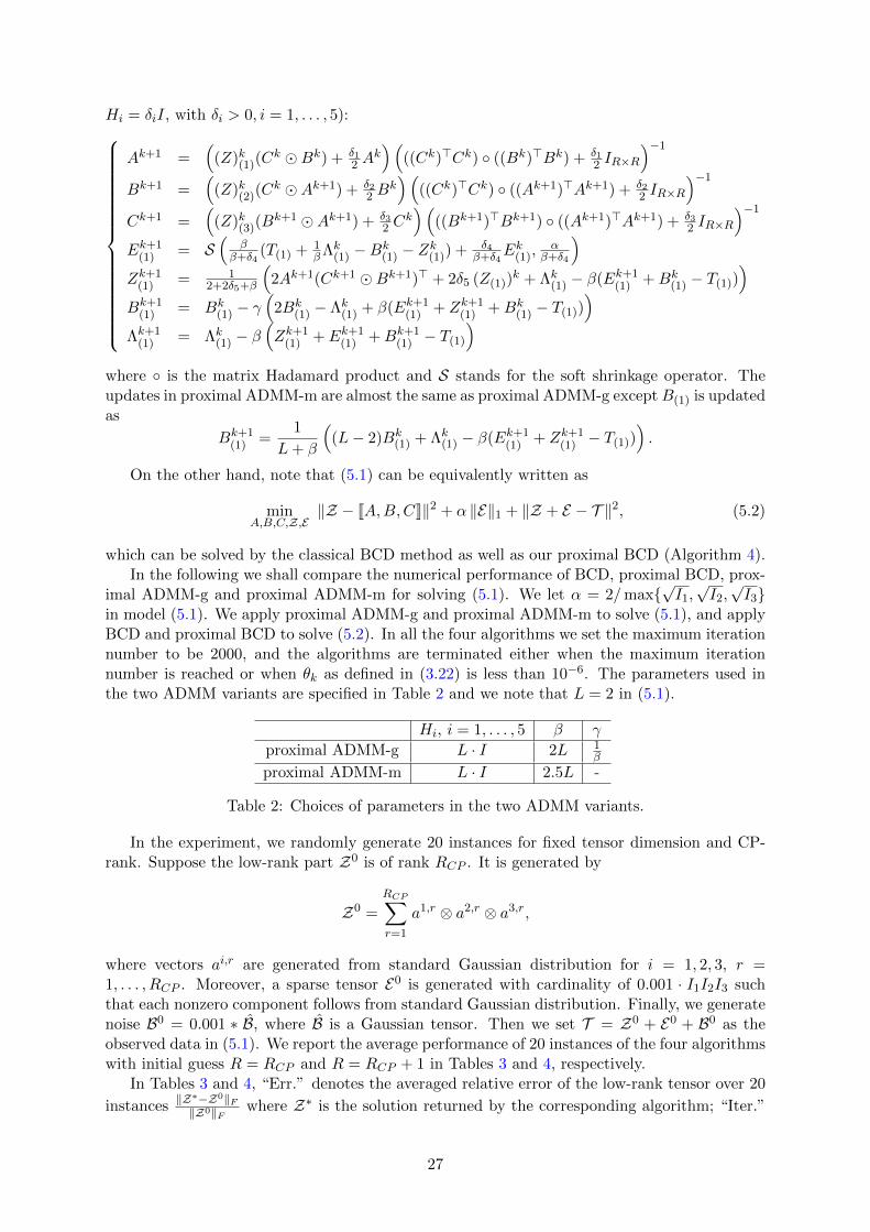
Hi = δiI, with δi > 0, i = 1, . . . , 5):
Ak+1 =(
(Z)k(1)(Ck �Bk) + δ1
2 Ak)(
((Ck)>Ck) ◦ ((Bk)>Bk) + δ12 IR×R
)−1
Bk+1 =(
(Z)k(2)(Ck �Ak+1) + δ2
2 Bk)(
((Ck)>Ck) ◦ ((Ak+1)>Ak+1) + δ22 IR×R
)−1
Ck+1 =(
(Z)k(3)(Bk+1 �Ak+1) + δ3
2 Ck)(
((Bk+1)>Bk+1) ◦ ((Ak+1)>Ak+1) + δ32 IR×R
)−1
Ek+1(1) = S
(β
β+δ4(T(1) + 1
βΛk(1) −Bk(1) − Z
k(1)) + δ4
β+δ4Ek(1),
αβ+δ4
)Zk+1
(1) = 12+2δ5+β
(2Ak+1(Ck+1 �Bk+1)> + 2δ5 (Z(1))
k + Λk(1) − β(Ek+1(1) +Bk
(1) − T(1)))
Bk+1(1) = Bk
(1) − γ(
2Bk(1) − Λk(1) + β(Ek+1
(1) + Zk+1(1) +Bk
(1) − T(1)))
Λk+1(1) = Λk(1) − β
(Zk+1
(1) + Ek+1(1) +Bk+1
(1) − T(1)
)where ◦ is the matrix Hadamard product and S stands for the soft shrinkage operator. Theupdates in proximal ADMM-m are almost the same as proximal ADMM-g except B(1) is updatedas
Bk+1(1) =
1
L+ β
((L− 2)Bk
(1) + Λk(1) − β(Ek+1(1) + Zk+1
(1) − T(1))).
On the other hand, note that (5.1) can be equivalently written as
minA,B,C,Z,E
‖Z − JA,B,CK‖2 + α ‖E‖1 + ‖Z + E − T ‖2, (5.2)
which can be solved by the classical BCD method as well as our proximal BCD (Algorithm 4).In the following we shall compare the numerical performance of BCD, proximal BCD, prox-
imal ADMM-g and proximal ADMM-m for solving (5.1). We let α = 2/max{√I1,√I2,√I3}
in model (5.1). We apply proximal ADMM-g and proximal ADMM-m to solve (5.1), and applyBCD and proximal BCD to solve (5.2). In all the four algorithms we set the maximum iterationnumber to be 2000, and the algorithms are terminated either when the maximum iterationnumber is reached or when θk as defined in (3.22) is less than 10−6. The parameters used inthe two ADMM variants are specified in Table 2 and we note that L = 2 in (5.1).
Hi, i = 1, . . . , 5 β γ
proximal ADMM-g L · I 2L 1β
proximal ADMM-m L · I 2.5L -
Table 2: Choices of parameters in the two ADMM variants.
In the experiment, we randomly generate 20 instances for fixed tensor dimension and CP-rank. Suppose the low-rank part Z0 is of rank RCP . It is generated by
Z0 =
RCP∑r=1
a1,r ⊗ a2,r ⊗ a3,r,
where vectors ai,r are generated from standard Gaussian distribution for i = 1, 2, 3, r =1, . . . , RCP . Moreover, a sparse tensor E0 is generated with cardinality of 0.001 · I1I2I3 suchthat each nonzero component follows from standard Gaussian distribution. Finally, we generatenoise B0 = 0.001 ∗ B, where B is a Gaussian tensor. Then we set T = Z0 + E0 + B0 as theobserved data in (5.1). We report the average performance of 20 instances of the four algorithmswith initial guess R = RCP and R = RCP + 1 in Tables 3 and 4, respectively.
In Tables 3 and 4, “Err.” denotes the averaged relative error of the low-rank tensor over 20
instances ‖Z∗−Z0‖F‖Z0‖F where Z∗ is the solution returned by the corresponding algorithm; “Iter.”
27
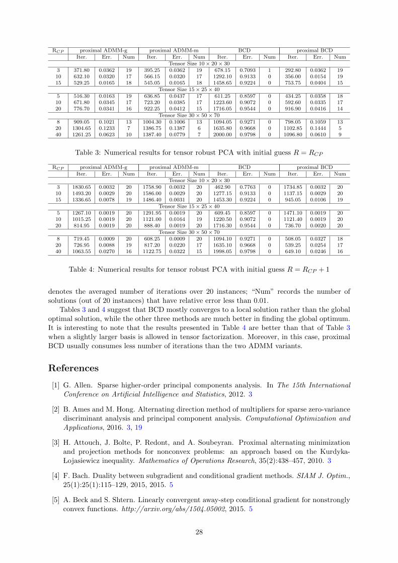
RCP proximal ADMM-g proximal ADMM-m BCD proximal BCDIter. Err. Num Iter. Err. Num Iter. Err. Num Iter. Err. Num
Tensor Size 10× 20× 303 371.80 0.0362 19 395.25 0.0362 19 678.15 0.7093 1 292.80 0.0362 1910 632.10 0.0320 17 566.15 0.0320 17 1292.10 0.9133 0 356.00 0.0154 1915 529.25 0.0165 18 545.05 0.0165 18 1458.65 0.9224 0 753.75 0.0404 15
Tensor Size 15× 25× 405 516.30 0.0163 19 636.85 0.0437 17 611.25 0.8597 0 434.25 0.0358 1810 671.80 0.0345 17 723.20 0.0385 17 1223.60 0.9072 0 592.60 0.0335 1720 776.70 0.0341 16 922.25 0.0412 15 1716.05 0.9544 0 916.90 0.0416 14
Tensor Size 30× 50× 708 909.05 0.1021 13 1004.30 0.1006 13 1094.05 0.9271 0 798.05 0.1059 1320 1304.65 0.1233 7 1386.75 0.1387 6 1635.80 0.9668 0 1102.85 0.1444 540 1261.25 0.0623 10 1387.40 0.0779 7 2000.00 0.9798 0 1096.80 0.0610 9
Table 3: Numerical results for tensor robust PCA with initial guess R = RCP
RCP proximal ADMM-g proximal ADMM-m BCD proximal BCDIter. Err. Num Iter. Err. Num Iter. Err. Num Iter. Err. Num
Tensor Size 10× 20× 303 1830.65 0.0032 20 1758.90 0.0032 20 462.90 0.7763 0 1734.85 0.0032 2010 1493.20 0.0029 20 1586.00 0.0029 20 1277.15 0.9133 0 1137.15 0.0029 2015 1336.65 0.0078 19 1486.40 0.0031 20 1453.30 0.9224 0 945.05 0.0106 19
Tensor Size 15× 25× 405 1267.10 0.0019 20 1291.95 0.0019 20 609.45 0.8597 0 1471.10 0.0019 2010 1015.25 0.0019 20 1121.00 0.0164 19 1220.50 0.9072 0 1121.40 0.0019 2020 814.95 0.0019 20 888.40 0.0019 20 1716.30 0.9544 0 736.70 0.0020 20
Tensor Size 30× 50× 708 719.45 0.0009 20 608.25 0.0009 20 1094.10 0.9271 0 508.05 0.0327 1820 726.95 0.0088 19 817.20 0.0220 17 1635.10 0.9668 0 539.25 0.0254 1740 1063.55 0.0270 16 1122.75 0.0322 15 1998.05 0.9798 0 649.10 0.0246 16
Table 4: Numerical results for tensor robust PCA with initial guess R = RCP + 1
denotes the averaged number of iterations over 20 instances; “Num” records the number ofsolutions (out of 20 instances) that have relative error less than 0.01.
Tables 3 and 4 suggest that BCD mostly converges to a local solution rather than the globaloptimal solution, while the other three methods are much better in finding the global optimum.It is interesting to note that the results presented in Table 4 are better than that of Table 3when a slightly larger basis is allowed in tensor factorization. Moreover, in this case, proximalBCD usually consumes less number of iterations than the two ADMM variants.
References
[1] G. Allen. Sparse higher-order principal components analysis. In The 15th InternationalConference on Artificial Intelligence and Statistics, 2012. 3
[2] B. Ames and M. Hong. Alternating direction method of multipliers for sparse zero-variancediscriminant analysis and principal component analysis. Computational Optimization andApplications, 2016. 3, 19
[3] H. Attouch, J. Bolte, P. Redont, and A. Soubeyran. Proximal alternating minimizationand projection methods for nonconvex problems: an approach based on the Kurdyka- Lojasiewicz inequality. Mathematics of Operations Research, 35(2):438–457, 2010. 3
[4] F. Bach. Duality between subgradient and conditional gradient methods. SIAM J. Optim.,25(1):25(1):115–129, 2015, 2015. 5
[5] A. Beck and S. Shtern. Linearly convergent away-step conditional gradient for nonstronglyconvex functions. http://arxiv.org/abs/1504.05002, 2015. 5
28
[6] W. Bian and X. Chen. Worst-case complexity of smoothing quadratic regularization meth-ods for non-Lipschitzian optimization. SIAM Journal on Optimization, 23:1718–1741, 2013.3
[7] W. Bian and X. Chen. Feasible smoothing quadratic regularization method for box con-strained non-Lipschitz optimization. Technical Report, 2014. 3
[8] W. Bian, X. Chen, and Y. Ye. Complexity analysis of interior point algorithms for non-Lipschitz and nonconvex minimization. Mathematical Programming, 149:301–327, 2015.3
[9] J. Bolte, A. Daniilidis, and A. Lewis. The lojasiewicz inequality for nonsmooth suban-alytic functions with applications to subgradient dynamical systems. SIAM Journal onOptimization, 17:1205–1223, 2006. 3
[10] J. Bolte, A. Daniilidis, O. Ley, and L. Mazet. Characterizations of lojasiewicz inequalities:subgradient flows, talweg, convexity. Transactions of the American Mathematical Society,362(6):3319–3363, 2010. 3
[11] J. Bolte, S. Sabach, and M. Teboulle. Proximal alternating linearized minimization fornonconvex and nonsmooth problems. Mathematical Programming, 146:459–494, 2014. 3
[12] S. Boyd, N. Parikh, E. Chu, B. Peleato, and J. Eckstein. Distributed optimization andstatistical learning via the alternating direction method of multipliers. Foundations andTrends in Machine Learning, 3(1):1–122, 2011. 13
[13] K. Bredies. A forward-backward splitting algorithm for the minimization of non-smoothconvex functionals in Banach space. Inverse Problems, 25(1), 2009. 3
[14] K. Bredies, D. A. Lorenz, and P. Maass. A generalized conditional gradient method andits connection to an iterative shrinkage method. Computational Optimization and Appli-cations, 42(2):173–193, 2009. 5
[15] E. J. Candes, M. B. Wakin, and S. P. Boyd. Enhancing sparsity by reweighted `1 mini-mization. Journal of Fourier analysis and applications, 14(5-6):877–905, 2008. 2
[16] C. Cartis, N. I. M. Gould, and Ph. L. Toint. On the complexity of steepest descent,Newton’s and regularized Newton’s methods for nonconvex unconstrained optimization.SIAM Journal on Optimization, 20(6):2833–2852, 2010. 6
[17] C. Cartis, N. I. M. Gould, and Ph. L. Toint. Adaptive cubic overestimation methods for un-constrained optimization. part ii: worst-case function-evaluation complexity. MathematicalProgramming, Series A, 130(2):295–319, 2011. 6
[18] C. Cartis, N. I. M. Gould, and Ph. L. Toint. An adaptive cubic regularization algorithmfor nonconvex optimization with convex constraints and its function-evaluation complexity.IMA Journal of Numerical Analysis, 2013. 6, 7
[19] X. Chen, D. Ge, Z. Wang, and Y. Ye. Complexity of unconstrained l2-lp minimization.Mathematical Programming, 143:371–383, 2014. 3
[20] O. Devolder, G. Francois, and Yu. Nesterov. First-order methods of smooth convex opti-mization with inexact oracle. Mathematical Programming, Ser. A, 146:37–75, 2014. 5
[21] J. Fan and R. Li. Variable selection via nonconcave penalized likelihood and its oracleproperties. Journal of the American statistical Association, 96(456):1348–1360, 2001. 2
29
[22] M. Frank and P. Wolfe. An algorithm for quadratic programming. Naval Research LogisticsQuarterly, 3:95–110, 1956. 5
[23] R. M. Freund and P. Grigas. New analysis and results for the Frank-Wolfe method.Mathematical Programming, 2013. 5
[24] D. Ge, R. He, and S. He. A three criteria algorithm for l2 − lp minimization problem withlinear constraints. Technical report, Shanghai University of Finance and Economics, 2014.3, 9
[25] S. Ghadimi, G. Lan, and H. Zhang. Mini-batch stochastic approximation methods fornonconvex stochastic composite optimization. Mathematical Programming, 2014. 3, 7
[26] P. Gong, C. Zhang, Z. Lu, J. Huang, and J. Ye. A general iterative shrinkage and thresh-olding algorithm for non-convex regularized optimization problems. In ICML, pages 37–45,2013. 4
[27] Z. Harchaoui, A. Juditsky, and A. Nemirovski. Conditional gradient algorithms for norm-regularized smooth convex optimization. Math. Program., 152:75–112, 2015. 5
[28] M. Hong. A distributed, asynchronous and incremental algorithm for nonconvex optimiza-tion: An ADMM based approach. http://arxiv.org/pdf/1412.6058v1.pdf, 2014. 19
[29] M. Hong. Decomposing linearly constrained nonconvex problems by a proximal primal dualapproach: Algorithms, convergence, and applications. https://arxiv.org/abs/1604.00543,2016. 3, 12, 13, 19
[30] M. Hong, Z.-Q. Luo, and M M. Razaviyayn. Convergence analysis of alternating directionmethod of multipliers for a family of nonconvex problems. SIAM Journal on Optimization,2015. 3, 13, 19
[31] M. Jaggi. Revisiting Frank-Wolfe: Projection-free sparse convex optimization. In ICML,2013. 5
[32] B. Jiang, F. Yang, and S. Zhang. Tensor and its Tucker core: the invariance relationships.arXiv preprint arXiv:1601.01469, 2016. 2
[33] K. Kurdyka. On gradients of functions definable in o-minimal structures. Annales del’institut Fourier, 146:769–783, 1998. 3
[34] G. Lan and Y. Zhou. Conditional gradient sliding for convex optimization. 2014. 5
[35] G. Li and T. K. Pong. Global convergence of splitting methods for nonconvex compositeoptimization. SIAM Journal on Optimization, 25(4):2434–2460, 2015. 3, 19
[36] T. Lin, S. Ma, and S. Zhang. Global convergence of unmodified 3-block ADMM for a classof convex minimization problems. Preprint http://arxiv.org/abs/1505.04252, 2015. 13
[37] T. Lin, S. Ma, and S. Zhang. Iteration complexity analysis of multi-block ADMM for afamily of convex minimization without strong convexity. Journal of Scientific Computing,2015. 13
[38] Y. Liu, S. Ma, Y. Dai, and S. Zhang. A smoothing SQP framework for a class of composite`q minimization over polyhedron. Mathematical Programming Series A, to appear, 2015. 3
[39] S. Lojasiewicz. Une propriete topologique des sous-ensembles analytiques reels, LesEquations aux Derivees Partielles. Editions du centre National de la Recherche Scien-tifique, Paris, 1963. 3
30
[40] S. Lojasiewicz. Clarke subgradients of stratifiable functions. SIAM Journal on Optimiza-tion, 18:556–572, 2007. 3
[41] R. Luss and M. Teboulle. Conditional gradient algorithms for rank one matrix approxima-tions with a sparsity constraint. SIAM Review, 55:65–98, 2013. 8
[42] C. Mu, Y. Zhang, J. Wright, and D. Goldfarb. Scalable robust matrix recovery: Frank-Wolfe meets proximal methods. arXiv preprint arXiv:1403.7588v1, 2014. 5
[43] Y. E. Nesterov. Introductory lectures on convex optimization. Applied Optimization. K-luwer Academic Publishers, Boston, MA, 2004. 6
[44] R. T. Rockafellar and R. Wets. Variational Analysis. Springer, Volume 317 of Grundlehrender Mathematischen Wissenschafte, 1998. 11
[45] Y. Shen, Z. Wen, and Y. Zhang. Augmented Lagrangian alternating direction method formatrix separation based on low-rank factorization. Optimization Methods and Software,29(2):239–263, 2014. 2
[46] F. Wang, W. Cao, and Z. Xu. Convergence of multiblock Bregman ADMM for nonconvexcomposite problems. http://arxiv.org/abs/1505.03063, 2015. 3
[47] Y. Wang, W. Yin, and J. Zeng. Global convergence of ADMM in nonconvex nonsmoothoptimization. http://arxiv.org/abs/1511.06324, 2015. 3
[48] Y. Xu. Alternating proximal gradient method for sparse nonnegative Tucker decomposition.Mathematical Programming Computation, 7(1):39–70, 2015. 2
[49] L. Yang, T.K. Pong, and X. Chen. Alternating direction method of multipliers for aclass of nonconvex and nonsmooth problems with applications to background/foregroundextraction. Preprint available at http://arxiv.org/abs/1506.07029, 2016. 3
[50] C.-H. Zhang. Nearly unbiased variable selection under minimax concave penalty. TheAnnals of Statistics, pages 894–942, 2010. 2
[51] T. Zhang. Analysis of multi-stage convex relaxation for sparse regularization. The Journalof Machine Learning Research, 11:1081–1107, 2010. 2
[52] T. Zhang. Multi-stage convex relaxation for feature selection. Bernoulli, 19(5B):2277–2293,2013. 2
31


![[Poster Presentation] Nonconvex Optimization …rhayakawa/paper/RCC2019...[Poster Presentation] Nonconvex Optimization Based Algorithm for Discrete-Valued Vector Reconstruction Ryo](https://img.pdfslide.net/doc/110x75/5f0609c97e708231d415fbb0/poster-presentation-nonconvex-optimization-rhayakawapaperrcc2019-poster.jpg)