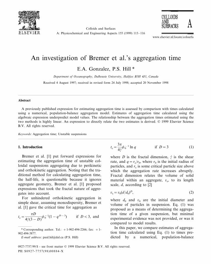
Colloids and Surfaces

A: Physicochemical and Engineering Aspects 155 (1999) 113–116

An investigation of Bremer et al.’s aggregation time

E.A. Gonzalez, P.S. Hill *Department of Oceanography, Dalhousie Uni6ersity, Halifax B3H 4J1, Canada

Received 4 August 1997; received in revised form 24 July 1998; accepted 20 November 1998

Abstract

A previously published expression for estimating aggregation time is assessed by comparison with times calculatedusing a numerical, population-balance aggregation model. Estimates of aggregation time calculated using thealgebraic expression underpredict model values. The relationship between the aggregation times estimated using thetwo methods is highly linear. An expression to directly relate the two estimates is derived. © 1999 Elsevier ScienceB.V. All rights reserved.

Keywords: Aggregation time; Unstable suspensions

www.elsevier.nl/locate/colsurfa

1. Introduction

Bremer et al. [1] put forward expressions forestimating the aggregation time of unstable col-loidal suspensions aggregating due to perikineticand orthokinetic aggregation. Noting that the tra-ditional method for calculating aggregation time,the half-life, is questionable because it ignoresaggregate geometry, Bremer et al. [1] proposedexpressions that took the fractal nature of aggre-gates into account.

For unhindered orthokinetic aggregation insimple shear, assuming monodispersity, Bremer etal. [1] gave the critical time for aggregation as

tc=pD

4g; (3−D)f0

−1(1−qD−3) if DB3, and

tc=3p

4g; f0−1 ln q if D=3 (1)

where D is the fractal dimension, g; is the shearrate, and q=rc/r0, where r0 is the initial radius ofparticles, and rc is some critical particle size abovewhich the aggregation rate increases abruptly.Fractal dimension relates the volume of solidmaterial within an aggregate, 6s, to its lengthscale, d, according to [2]

6s=60(d/d0)D, (2)

where d0 and 60 are the initial diameter andvolume of particles in suspension. Eq. (1) wasproposed as a means of determining the aggrega-tion time of a given suspension, but minimalexperimental evidence was not provided, or was itcompared to model results.

In this paper, we compare estimates of aggrega-tion time calculated using Eq. (1) to times pre-dicted by a numerical, population-balance

* Corresponding author. Tel.: +1-902-494-2266; fax: +1-902-494-3877.

E-mail address: paul.hil@dal.ca (P.S. Hill)

0927-7757/99/$ - see front matter © 1999 Elsevier Science B.V. All rights reserved.

PII: S0927 -7757 (98 )00884 -X

E.A. Gonzalez, P.S. Hill / Colloids and Surfaces A: Physicochem. Eng. Aspects 155 (1999) 113–116114

aggregation model. These models predict anabrupt transition from the unaggregated to theaggregated state [3–5] (Fig. 1). We define theaggregation time as the time at which the medianmass diameter of particles in suspension, d50, ismidway between its minimum and maximumvalue.

2. Methods

2.1. Sectional model

In a review of zero-order coagulation models[6], models of the type proposed by Batterham etal. [7] were found to give the best overall perfor-mance. (more recent modeling attempts [8] haveimproved upon [7]). The model of Batterham etal. [7] conserves particle mass, and most closelyapproximates analytical solutions of the aggrega-tion equation. Also, its form is computationallyefficient.

The model is a discrete geometric sectionalmodel in which the particle-size distribution isapproximated by a histogram with a constant sizedistribution in each cell or section; section widthsincrease geometrically with particle volume. Thesize distribution is further simplified by assumingthat only particles of discrete volumes exist, suchthat particles in section j have volume equal to2 j−160 where 60 is the initial mean volume ofparticles in suspension.

According to the population balance approach,an ordinary differential equation expressing therate of change of dimensionless particle number,n, with dimensionless time, t, is required for eachsection. For section i, the model states

dni

dt=

38

b. i−2, i−1 ni−2 ni−1+34

b. i−1, ini−1 ni

+b. i−1, i−1 ni−12

+ %i−2

m=1

2i+2m

2i b. i, mni nm− %h−1

m=1

qi, m b. i, mni nm

qi,m=2, if i=m

qi,m=1, otherwise (3)

where for the sections below, only the indicatedterms are used:

i=1, fifth term

i=2, second, third and fifth terms

i=h, first and third terms.

The coefficients b. are dimensionless encounter-rate kernels, h is the number of sections, and

t=b1, 1 N0 t, (4)

where b1,1 is the encounter-rate kernel for parti-cles in the first section, N0 is the initial particlenumber concentration, and t is time. Note thatsince there are no explicit disaggregation terms inthe model, nor are there other loss terms forsection h, material accumulates in the largest sec-tion. For a discussion of each term in Eq. (3), see[9].

Dimensionless encounter-rate kernels b. , aredefined as

b. i, j=bi, j/b1,1 (5)

where bi, j is the encounter-rate kernel for particlesi and j. For orthokinetic aggregation in simpleshear [10]

b. i, j=43

g; (ri+rj)3 (6)

where ri, rj are the radii of interacting particles,and g; is the shear rate. To include the fractalnature of aggregates, b. is calculated using the

Fig. 1. Model output [5] showing nondimensional mediandiameter (d50/d0) as a function of nondimensional time (t).

E.A. Gonzalez, P.S. Hill / Colloids and Surfaces A: Physicochem. Eng. Aspects 155 (1999) 113–116 115

Fig. 2. Comparison of dimensionless aggregation times calculated using the model (tM) and Eq. (1) (tE). The number of sections in(a), (b) and (c) is 12, 16 and 20, respectively. For all regression lines, R2\0.99.

diameter that an aggregate in section j must haveif its solids volume is 2 j−160. Rearranging Eq. (2)for aggregate diameter gives

d=d0(6s/60)1/D,

or

dj=d0(2 j−1)1/D. (7)

Therefore, for a given value of h, the maximumparticle diameter varies depending on the fractaldimension.

To simplify notation, the dimensionless aggre-gation time predicted by the model is representedby tM.

2.2. Estimate of aggregation time

To implement Eq. (1), the volume fraction ofparticles is given by

f0=N060,

where N0 is the initial number concentration ofparticle. The aggregation time estimated using Eq.(1) is nondimensionalized as in Eq. (4), and isgiven the symbol tE.

2.3. Analysis

Four model inputs affect aggregation time: ini-tial particle size, r0, shear rate, g; , fractal dimen-sion, D, and the size of the largest allowableparticle, which is determined by the number ofsections used, h. Of these, the variation in only

two, D and h, can affect dimensionless aggrega-tion time. Because encounter-rate coefficients arenondimensionalized with respect to orthokineticencounter between particles of size r0, dimension-less aggregation times for all values of shear rateand initial particle size with respect to D and hcollapse onto a single curve. Therefore, aggrega-tion times are calculated for a range of particlesizes, h={10, 12, 14, 16, 18, 20}, and fractaldimensions, D={3.0, 2.9, 2.8, 2.7, 2.6, 2.5, 2.4,2.3, 2.2, 2.1, 2.0}.

The model was run using a small time-step, andat each step, the nondimensional median diameterwas calculated for the particle size distribution,with dmax determined using Eq. (7) for j=h. Oncethe nondimensional median diameter exceeded thevalue d50=dmax+d0/2D0, linear interpolation was

Fig. 3. Comparison of dimensionless aggregation times forturbulent shear encounter calculated using the model (tM) andEq. (1) (tE) for all cases.

E.A. Gonzalez, P.S. Hill / Colloids and Surfaces A: Physicochem. Eng. Aspects 155 (1999) 113–116116

used to determine the nondimensional aggrega-tion time. This value was compared against thatgiven by Eq. (1), using q=dmax+d0/2d0

3. Results and discussion

Bremer et al.’s [1] estimation gives dimension-less aggregation times that are on the same orderas those predicted by the model, and the relation-ship between the two is highly linear (Fig. 2).Each point represents a different fractal dimen-sion; t increases with D.

It is rather surprising that tE should predict tM

so well, given that Batterham et al.’s [7] modelpredicts that suspensions become highly dispersedwithin a very short time; the assumption thatsuspensions remain monodispersed is invalid.Nevertheless, the formulation of Bremer et al. [1]manages to capture the overall behaviour of thesuspension. The assumption of monodispersitymeans that there is only one loss rate to considerat any time, but the size of particles in suspensionis constantly increasing, as is the encounter rate.

Estimates of aggregation time are always longerthan model results. Modeled size distributionsshow that small numbers of large particles areformed shortly after the onset of aggregation.Although rare, these large particles have highaggregation rates with smaller particles since en-counter rate is a strong function of particle size(see Eq. (6)). The overall aggregation time, there-fore, is decreased as a result. Because Bremer etal.’s [1] expression is based on a monodispersedsize distribution, the effect of very large particlesis removed.

Because the relationship between tM and tE forall cases is linear (Fig. 3), a first-order multiplelinear regression equation is determined to di-rectly relate the two. Using Matlab, the best fit is

tM=0.84tE−0.59D−0.044h−0.84, (8)

where h can be calculated using

h=D log2(dmax/d0)+1. (9)

This model should be restricted to the range ofvalues of h and D used to develop Eq. (8), i.e.105h520 and 2.05D53.0.

4. Conclusions

Bremer et al.’s [1] expression provides an easymethod for estimating aggregation time. Usedwith the correction given in Eq. (8), it predictsaggregation times with the accuracy of a popula-tion-balance, aggregation model, without thecomputational effort required to run such amodel.

References

[1] L.G.B. Bremer, P. Walstra, T. van Vliet, Colloids Surf. A:Physicochem. Eng. Aspects 99 (1995) 121.

[2] B.E. Logan, D.G. Wilkinson, Limnol. Oceanogr. 35(1990) 130.

[3] W. Lick, J. Lick, C.K. Ziegler, Hydrobiologia 235/236(1992) 1.

[4] W. Lick, H. Huang, in: A.J. Mehta (Ed.), Nearshore andEstuarine Cohesive Sediment Transport, AmericanGeophysical Union, Washington, DC, 1993, p. 21.

[5] P.S. Hill, A.R.M. Nowell, J. Geophys. Res. 100 (1995)749.

[6] M. Kostoglou, A.J. Karabelas, J. Colloid Interface Sci.163 (1994) 420.

[7] R.J. Batterham, J.S. Hall, G. Barton, in: Proceedings, 3rdInternational Symposium on Agglomeration, Nurnberg,Federal Republic of Germany, 1981, pp. A136.

[8] S. Kumar, D. Ramkrishna, Chem. Eng. Sci. 51 (1996)1311.

[9] P.T.L. Koh, J.R.G Andrews, P.H.T. Uhlherr, Chem. Eng.Sci. 42 (1987) 353.

[10] M. Smoluchowski, Z. Phys. Chem. 92 (1917) 129.

.