Analysis of a hydrostatic drive wind turbine for improved

AIMS Energy, 6(6): 908–925.

DOI: 10.3934/energy.2018.6.908

Received: 19 August 2018

Accepted: 21 October 2018

Published: 26 October 2018

http://www.aimspress.com/journal/energy

Research article

Analysis of a hydrostatic drive wind turbine for improved annual

energy production

Majid Deldar1, Afshin Izadian

2 and Sohel Anwar

3,*

1 Meggitt Control Systems, Los Angeles, CA 91605, USA 2 Energy Systems and Power Electronics Lab, Purdue School of Engineering and Technology,

Indianapolis, Indiana, USA 3 Department of Mechanical and Energy Engineering, Purdue School of Engineering and Technology

Indianapolis, Indiana, USA

* Correspondence: Email: [email protected]; Tel: +13172747640.

Abstract: This paper presents an analysis on ways to improve the annual energy production (AEP) of

a wind turbine utilizing a drivetrain that operates based on the hydrostatic transmission. The system

configuration of such a drivetrain is explained in details and a comparison of operation and

characteristics with existing drivetrains is provided. AEP was estimated for these configurations

through appropriate dynamic modeling and operational efficiency optimization. Optimal selection of a

number of design variables and system parameters contributed to the improvements in the AEP.

Findings of this study demonstrate that the proposed hydrostatic drivetrain improves the AEP of

a 750 kW turbine by up to +8% when compared with a geared wind turbine. The AEP improvements of

the hydrostatic drive wind turbine were more than 10% for a 1.5 MW system over geared configuration.

It is also demonstrated that the efficiency of power generation can be improved under various wind

speeds. The suitable selection of synchronous speed of the generator directly improves the efficiency

of operation by up to 35% at low wind speeds. An efficiency improvement was also observed under

higher operating pressures and longer turbine blades.

Keywords: hydrostatic drivetrain; governing equations; efficiency enhancement; system

characteristics; annual energy production

mailto:[email protected]

909

AIMS Energy Volume 6, Issue 6, 908–925.

1. Introduction

By 2030, the wind energy is planned to cover significant share of the US energy [1]. Improving

the performance of wind turbine operation results in a higher energy production over time.

Conventional gearbox system transmits the power from a high torque-low speed rotor shaft to a low

torque-high speed generator shaft. This subassembly is heavy and expensive [2] causing long failure

downtime [3]. The variable speed on the generator shaft raises the need for a power electronic

converter to adjust the frequency variations. However, hydrostatic transmission system (HTS) can be

an alternative power transmission with inherent advantages. The system introduced in this paper is

comprised of a fixed displacement pump coupled with the rotor within the nacelle and a variable

displacement motor coupled with a generator on the ground level.

In this configuration controlling the displacement of motor adjusts the transmission ratio which

consequently sets the generator speed to a synchronous speed. Therefore, the power electronic

converters can be eliminated from the drivetrain. To maintain the frequency, the displacement of the

hydraulic motor is controlled. The speed of hydraulic pump which varies by the variable speed of wind

can be controlled to track the maximum power point. The efficiency of HTS utilized in wind turbines

(HTSWT) specifically at low wind speed operations has been studied by Thul et al. [4] and

Schmitz el at. [5]. To maximize the transmission system efficiency, Schmitz suggests a switching

mechanism between two hardware configurations, one with smaller pumps and motors (set to have

high efficiency at low wind speeds) and one with larger pumps and motors (set to have high efficiency

at high wind speeds. However, the transition between the sets of low and high speed imposes large

breaking torque on hydrostatic components. Dutta [6] suggested an auxiliary pump to be used to store

pressurized flow in an accumulator. This stored energy can be released when wind speed is slightly

lower than rated speed. Although this approach can increase AEP, the issue of low efficiency at low

wind speeds has not been addressed. The effect of system parameters such as the synchronous speed of

the generator and the blade size as well as its operating conditions on the efficiency of hydrostatic wind

turbines have not been studied before.

In this paper, efficiency improvement techniques in a wind turbine drivetrain with hydrostatic

transmission system are investigated. The design of the turbine is optimized to achieve higher efficiency

resulting in an increased annual energy production (AEP). The AEP of the optimized wind turbine is

simulated and compared with conventional wind turbines with gearbox to demonstrate the benefits.

The paper is organized as follows: In section II, the hydrostatic transmission system is utilized for the

wind turbine drivetrain and the governing equations are shown. In section III, the effect of regional

operating conditions on the efficiency improvements is discussed. In section IV, the effect of synchronous

speed on the efficiency improvements are discussed. In section V, the effect of operating pressure and rotor

blade on the efficiency is discussed. The power generation and annual energy production are discussed in

sections VI and VII. A comparison is provided with the existing drivetrains in section VII.

2. Hydrostatic transmission system for wind turbine applications

Hydraulic pumps and motors are the key components of a hydrostatic circuit of power

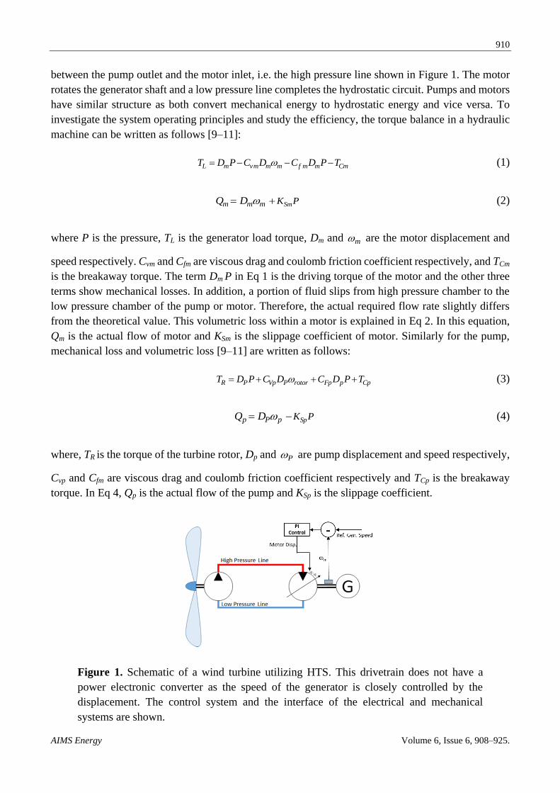
transmission. Figure 1 shows the proposed configuration of the hydrostatic drivetrain wind turbine

where the turbine shaft drives a hydraulic pump providing high pressure flow to the circuit. On the

motor side, the generator torque that imposes load on the hydraulic motor shaft induces pressure

910


between the pump outlet and the motor inlet, i.e. the high pressure line shown in Figure 1. The motor

rotates the generator shaft and a low pressure line completes the hydrostatic circuit. Pumps and motors

have similar structure as both convert mechanical energy to hydrostatic energy and vice versa. To

investigate the system operating principles and study the efficiency, the torque balance in a hydraulic

machine can be written as follows [9–11]:

L m vm m f m m CmmT D D C P TC DP (1)

Smm m m K PQ D (2)

where P is the pressure, TL is the generator load torque, Dm and m are the motor displacement and

speed respectively. Cvm and Cfm are viscous drag and coulomb friction coefficient respectively, and TCm

is the breakaway torque. The term Dm P in Eq 1 is the driving torque of the motor and the other three

terms show mechanical losses. In addition, a portion of fluid slips from high pressure chamber to the

low pressure chamber of the pump or motor. Therefore, the actual required flow rate slightly differs

from the theoretical value. This volumetric loss within a motor is explained in Eq 2. In this equation,

Qm is the actual flow of motor and KSm is the slippage coefficient of motor. Similarly for the pump,

mechanical loss and volumetric loss [9–11] are written as follows:

R P rotorVp P Fp p CpT D C DP C D P T (3)

Spp pP K PQ D (4)

where, TR is the torque of the turbine rotor, Dp and P are pump displacement and speed respectively,

Cvp and Cfm are viscous drag and coulomb friction coefficient respectively and TCp is the breakaway

torque. In Eq 4, Qp is the actual flow of the pump and KSp is the slippage coefficient.

Figure 1. Schematic of a wind turbine utilizing HTS. This drivetrain does not have a

power electronic converter as the speed of the generator is closely controlled by the

displacement. The control system and the interface of the electrical and mechanical

systems are shown.

911


3. Effect of regional operating conditions on overall efficiency

From motor and pump models 1–4, it can be seen that the energy conversion efficiency is

influenced by the mechanical and volumetric losses. The mechanical losses are viscous drag, coulomb

friction and breakaway torque. Viscous drag is caused by the fluid shear between two parts having

relative motion. The coulomb friction is due to contact between two metal surfaces such as bearing and

shaft and the breakaway torque is caused by sealing friction. Overall efficiency of a pump and a motor

including losses [9–11] are formulated as follows:

1

,

1p

S p

p

c pv p fp

p

K

A AT P

AC CD P

(5)

1

,

1m

cmvm f m

m m

S m

TBC C

D pB

K P

B

(6)

where P

and m

are the overall efficiencies of pump and motor respectively and is the dynamic

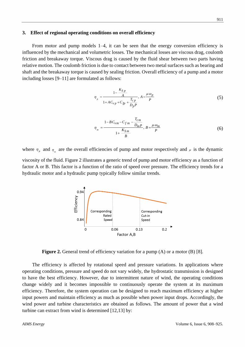
viscosity of the fluid. Figure 2 illustrates a generic trend of pump and motor efficiency as a function of

factor A or B. This factor is a function of the ratio of speed over pressure. The efficiency trends for a

hydraulic motor and a hydraulic pump typically follow similar trends.

Figure 2. General trend of efficiency variation for a pump (A) or a motor (B) [8].

The efficiency is affected by rotational speed and pressure variations. In applications where

operating conditions, pressure and speed do not vary widely, the hydrostatic transmission is designed

to have the best efficiency. However, due to intermittent nature of wind, the operating conditions

change widely and it becomes impossible to continuously operate the system at its maximum

efficiency. Therefore, the system operation can be designed to reach maximum efficiency at higher

input powers and maintain efficiency as much as possible when power input drops. Accordingly, the

wind power and turbine characteristics are obtained as follows. The amount of power that a wind

turbine can extract from wind is determined [12,13] by:

912


321

2pp C VR ,

(7)

where p is the rotor power, ρ is the air density, Cp is the power coefficient of turbine, R is the radius of

rotor, V is the instantaneous wind speed, and pR

V

is the instantaneous tip-speed-ratio of the rotor.

Considering Rp

pT

, the rotor torque can be expressed as follows:

52

3

1

2R p pC

RT

(8)

The rotor driving torque equals the braking torque applied on the pump shaft as p RT T , where

p

pPmech

D PT

, with

.P mech being the mechanical efficiency of the pump. Hence, the operating pressure of

the transmission fluid becomes proportional to the square of rotor shaft speed as follows:

251

2p

p

Pmechopt p

CR

PD

(9)

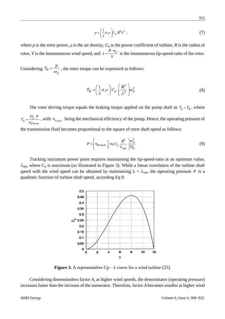
Tracking maximum power point requires maintaining the tip-speed-ratio at an optimum value,

opt, where Cp is maximum (as illustrated in Figure 3). While a linear correlation of the turbine shaft

speed with the wind speed can be obtained by maintaining = opt, the operating pressure P is a

quadratic function of turbine shaft speed, according Eq 9.

Figure 3. A representative Cp— curve for a wind turbine [25].

Considering dimensionless factor A, at higher wind speeds, the denominator (operating pressure)

increases faster than the increase of the numerator. Therefore, factor A becomes smaller at higher wind

913


speeds. This creates an optimum operation region as illustrated in Figure 2. In this optimum region, the

operating efficiency uniformly increases as the wind speed increases from the cut-in to the rated wind

speed where at it reaches the maximum efficiency within the range.

In factor B, which determines motor efficiency, the numerator is constant since motor speed is

desired to be maintained regardless of the wind speed. Pressure varies quadratic with wind speed,

hence, the value of factor B decreases faster at higher wind speed. This suggests that motors follow a

similar operational planning to the pump.

In this section, it was explained that the efficiency of hydrostatic transmission depends on the

operating conditions. To achieve higher efficiencies at low wind speeds, the characteristics of the

turbine (prime-mover) and the generator (load) must be considered in conjunction with HTS operation

characteristics. Therefore, in the next sections, the efficiency is measured against the generator speed

and the operating pressure variations.

4. Effect of generator’s synchronous speed on the overall efficiency

To increase the overall energy conversion efficiency, both mechanical efficiency .mech

, and the

volumetric efficiency vol

should be improved. Hydrostatic parameters that affect the efficiency are:

Pressure, pump/motor speeds, and displacements. Pump displacement is a constant value but its speed

is controlled to maintain the optimum tip-speed-ratio. Thus, this parameter cannot be controlled for

efficiency improvement. Effects of motor displacement and pressure are analyzed here to suggest

approaches for efficiency improvements.

The motor efficiency as a function of motor displacement is strictly increasing as observed

in Eq 6. This means that larger motor displacement improves motor efficiency. The optimality of this

relationship between efficiency variations and motor displacement is derived using the following

partial derivative:

2

20

1

cm

m m

m S m

T P

D P

D K

B

(10a)

Also, the hydrostatic drivetrain efficiency is obtained as:

(10b)

The hydraulic flow rate is determined by pump speed. To maintain higher efficiency, the same

amount of flow, when received by the motor at a large displacement, exhibits a reduced shaft speed.

This imposes a larger number of pole pairs in the generator to maintain the 60 Hz frequency.

Considering high speed generators as reported in [7], when a 1500 rpm 50 Hz generator [5] or

an 1800 rpm 60 Hz generator was used, low efficiencies were reported at low wind speeds.

914


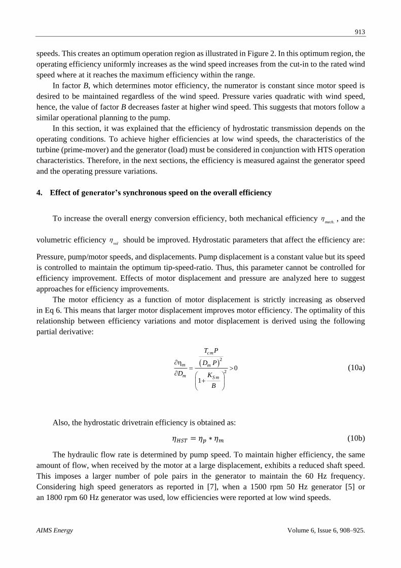
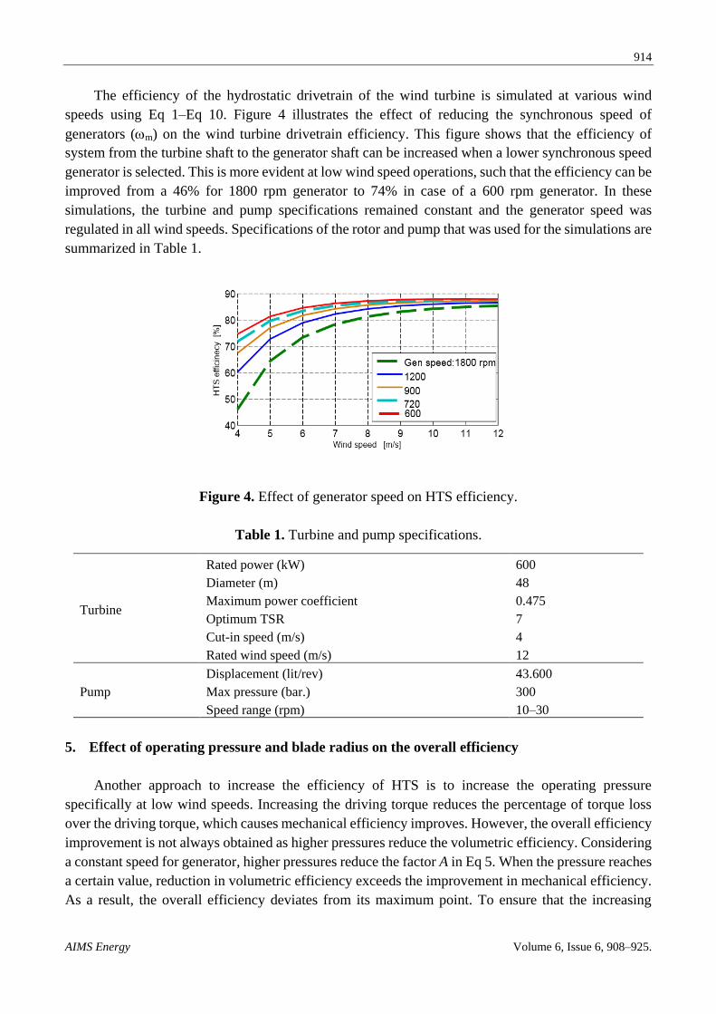
The efficiency of the hydrostatic drivetrain of the wind turbine is simulated at various wind

speeds using Eq 1–Eq 10. Figure 4 illustrates the effect of reducing the synchronous speed of

generators (m) on the wind turbine drivetrain efficiency. This figure shows that the efficiency of

system from the turbine shaft to the generator shaft can be increased when a lower synchronous speed

generator is selected. This is more evident at low wind speed operations, such that the efficiency can be

improved from a 46% for 1800 rpm generator to 74% in case of a 600 rpm generator. In these

simulations, the turbine and pump specifications remained constant and the generator speed was

regulated in all wind speeds. Specifications of the rotor and pump that was used for the simulations are

summarized in Table 1.

Figure 4. Effect of generator speed on HTS efficiency.

Table 1. Turbine and pump specifications.

Turbine

Rated power (kW) 600

Diameter (m) 48

Maximum power coefficient 0.475

Optimum TSR 7

Cut-in speed (m/s) 4

Rated wind speed (m/s) 12

Pump

Displacement (lit/rev) 43.600

Max pressure (bar.) 300

Speed range (rpm) 10–30

5. Effect of operating pressure and blade radius on the overall efficiency

Another approach to increase the efficiency of HTS is to increase the operating pressure

specifically at low wind speeds. Increasing the driving torque reduces the percentage of torque loss

over the driving torque, which causes mechanical efficiency improves. However, the overall efficiency

improvement is not always obtained as higher pressures reduce the volumetric efficiency. Considering

a constant speed for generator, higher pressures reduce the factor A in Eq 5. When the pressure reaches

a certain value, reduction in volumetric efficiency exceeds the improvement in mechanical efficiency.

As a result, the overall efficiency deviates from its maximum point. To ensure that the increasing

915


pressure improves the efficiency, a HTS is designated to operate in optimum regions shown in Figure 2.

The point of maximum efficiency is obtained analytically for the motor as follows (similar argument is

applied to the pump):

2

2

22

1

s m cm f m s mm m vm cm vm s m

m mm m

S m

K T C KD C T C K

P D PD P

P K

B

(11)

Sign of m

P

is determined by summation of the three terms in the numerator. The term

2

m m vm cm

m

D C T

D P

is always positive but its value is decreased at very high pressure since its denominator

increases quadratic with pressure. The term 2 vm smC K

P is also positive. However, the sign of the third

term, 2sm cm f m sm

m m

K T C K

D P

, can be either positive or negative. If the third term is positive, all of terms of

the partial derivate are positive and hence the overall efficiency of motor is a strictly increasing

function of pressure. However, Breakaway torque, Tcm and coulomb friction, Cvm are usually smaller

than the slippage coefficient, Ksm. Thus, the third term of the partial derivate can become negative. The

following argument illustrates that from low to a medium pressure, the overall efficiency is strictly

increasing with pressure.

At low to medium pressures:

20

20 0

20

m m vm cm

m

vm s m M

s m cm f m s m

m m

D C T

D P

C K

P P

K T C K

D P

(12)

At high pressure:

20

20 0

20

m m vm cm

m

vm s m M

s m cm f m s m

m m

D C T

D P

C K

P P

K T C K

D P

(13)

Hence, at high pressure, the drivetrain efficiency decreases as the pressure increases. From low to

medium pressure, the effect of mechanical efficiency overcomes the effect of volumetric efficiency.

However, at high pressure, the effect of volumetric efficiency dominates. The HTS should be designed

to operate in the region where efficiency increases by pressure.

To increase the pressure at low wind speeds, a large driving torque (prime-mover) is required.

Based on wind turbine power-torque characteristics, a larger swept area generates higher torque, as

indicated by Eq 7. Assuming that the wind turbine is designed for a fixed power rating, a larger swept

916


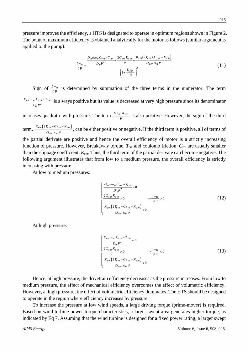
area helps the turbine reach the rated power at a lower wind speed. Figure 5 illustrates the correlation

between the blade radius, R, the rated wind speed and turbine rated power.

Figure 5. Power rating at different blade radius and rated wind speed.

As Figure 5 demonstrates, different combination of blade radius and rated wind speed might yield

a specific power rating. For instance, 1000 kW power can be generated with blade radius of 30 m in a

geographic area with rated wind speed of 11.4 m/s. It was observed in Eq 8 that the rotor torque was

proportional to 5R . Hence, the torque generation enhancement at low wind speeds can be achieved by

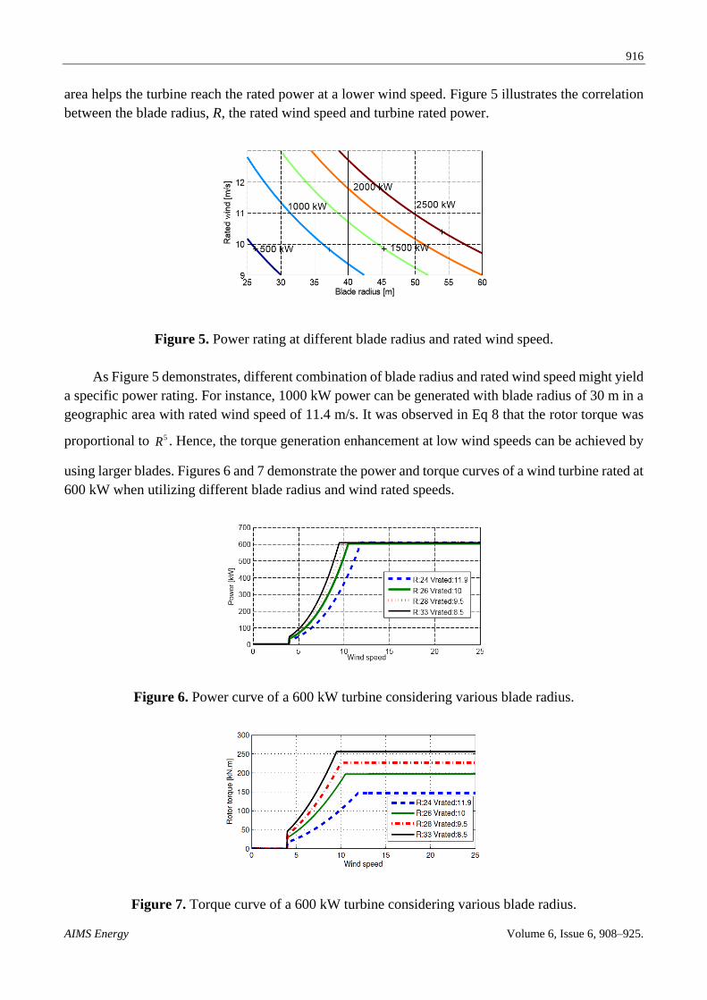
using larger blades. Figures 6 and 7 demonstrate the power and torque curves of a wind turbine rated at

600 kW when utilizing different blade radius and wind rated speeds.

Figure 6. Power curve of a 600 kW turbine considering various blade radius.

Figure 7. Torque curve of a 600 kW turbine considering various blade radius.

917


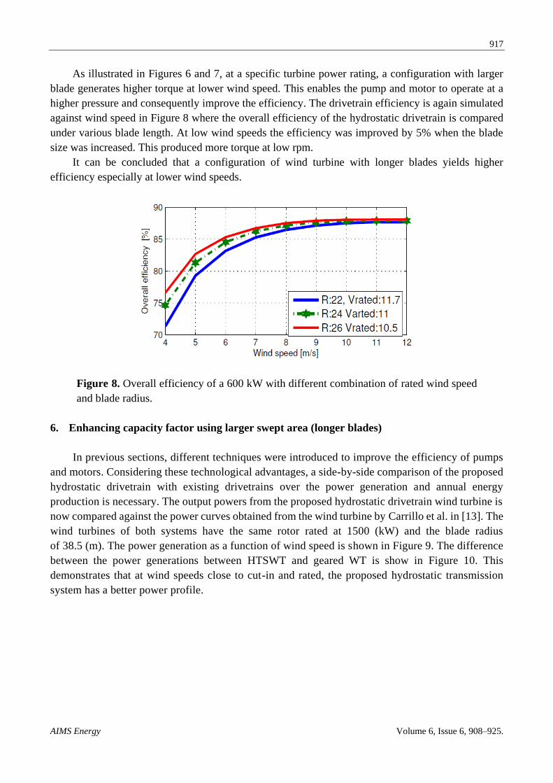
As illustrated in Figures 6 and 7, at a specific turbine power rating, a configuration with larger

blade generates higher torque at lower wind speed. This enables the pump and motor to operate at a

higher pressure and consequently improve the efficiency. The drivetrain efficiency is again simulated

against wind speed in Figure 8 where the overall efficiency of the hydrostatic drivetrain is compared

under various blade length. At low wind speeds the efficiency was improved by 5% when the blade

size was increased. This produced more torque at low rpm.

It can be concluded that a configuration of wind turbine with longer blades yields higher

efficiency especially at lower wind speeds.

Figure 8. Overall efficiency of a 600 kW with different combination of rated wind speed

and blade radius.

6. Enhancing capacity factor using larger swept area (longer blades)

In previous sections, different techniques were introduced to improve the efficiency of pumps

and motors. Considering these technological advantages, a side-by-side comparison of the proposed

hydrostatic drivetrain with existing drivetrains over the power generation and annual energy

production is necessary. The output powers from the proposed hydrostatic drivetrain wind turbine is

now compared against the power curves obtained from the wind turbine by Carrillo et al. in [13]. The

wind turbines of both systems have the same rotor rated at 1500 (kW) and the blade radius

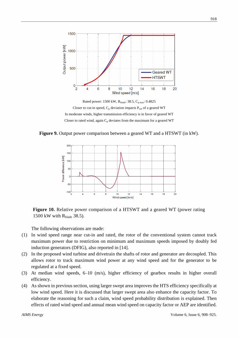
of 38.5 (m). The power generation as a function of wind speed is shown in Figure 9. The difference

between the power generations between HTSWT and geared WT is show in Figure 10. This

demonstrates that at wind speeds close to cut-in and rated, the proposed hydrostatic transmission

system has a better power profile.

918


Rated power: 1500 kW, Rblade: 38.5, Cp max: 0.4825

Closer to cut-in speed, Cp deviation impacts Pout of a geared WT

In moderate winds, higher transmission efficiency is in favor of geared WT

Closer to rated wind, again Cp deviates from the maximum for a geared WT

Figure 9. Output power comparison between a geared WT and a HTSWT (in kW).

Figure 10. Relative power comparison of a HTSWT and a geared WT (power rating

1500 kW with Rblade 38.5).

The following observations are made:

(1) In wind speed range near cut-in and rated, the rotor of the conventional system cannot track

maximum power due to restriction on minimum and maximum speeds imposed by doubly fed

induction generators (DFIG), also reported in [14].

(2) In the proposed wind turbine and drivetrain the shafts of rotor and generator are decoupled. This

allows rotor to track maximum wind power at any wind speed and for the generator to be

regulated at a fixed speed.

(3) At median wind speeds, 6–10 (m/s), higher efficiency of gearbox results in higher overall

efficiency.

(4) As shown in previous section, using larger swept area improves the HTS efficiency specifically at

low wind speed. Here it is discussed that larger swept area also enhance the capacity factor. To

elaborate the reasoning for such a claim, wind speed probability distribution is explained. Then

effects of rated wind speed and annual mean wind speed on capacity factor or AEP are identified.

919


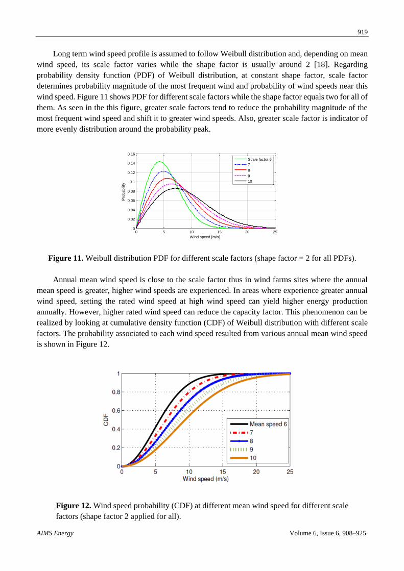
Long term wind speed profile is assumed to follow Weibull distribution and, depending on mean

wind speed, its scale factor varies while the shape factor is usually around 2 [18]. Regarding

probability density function (PDF) of Weibull distribution, at constant shape factor, scale factor

determines probability magnitude of the most frequent wind and probability of wind speeds near this

wind speed. Figure 11 shows PDF for different scale factors while the shape factor equals two for all of

them. As seen in the this figure, greater scale factors tend to reduce the probability magnitude of the

most frequent wind speed and shift it to greater wind speeds. Also, greater scale factor is indicator of

more evenly distribution around the probability peak.

Figure 11. Weibull distribution PDF for different scale factors (shape factor = 2 for all PDFs).

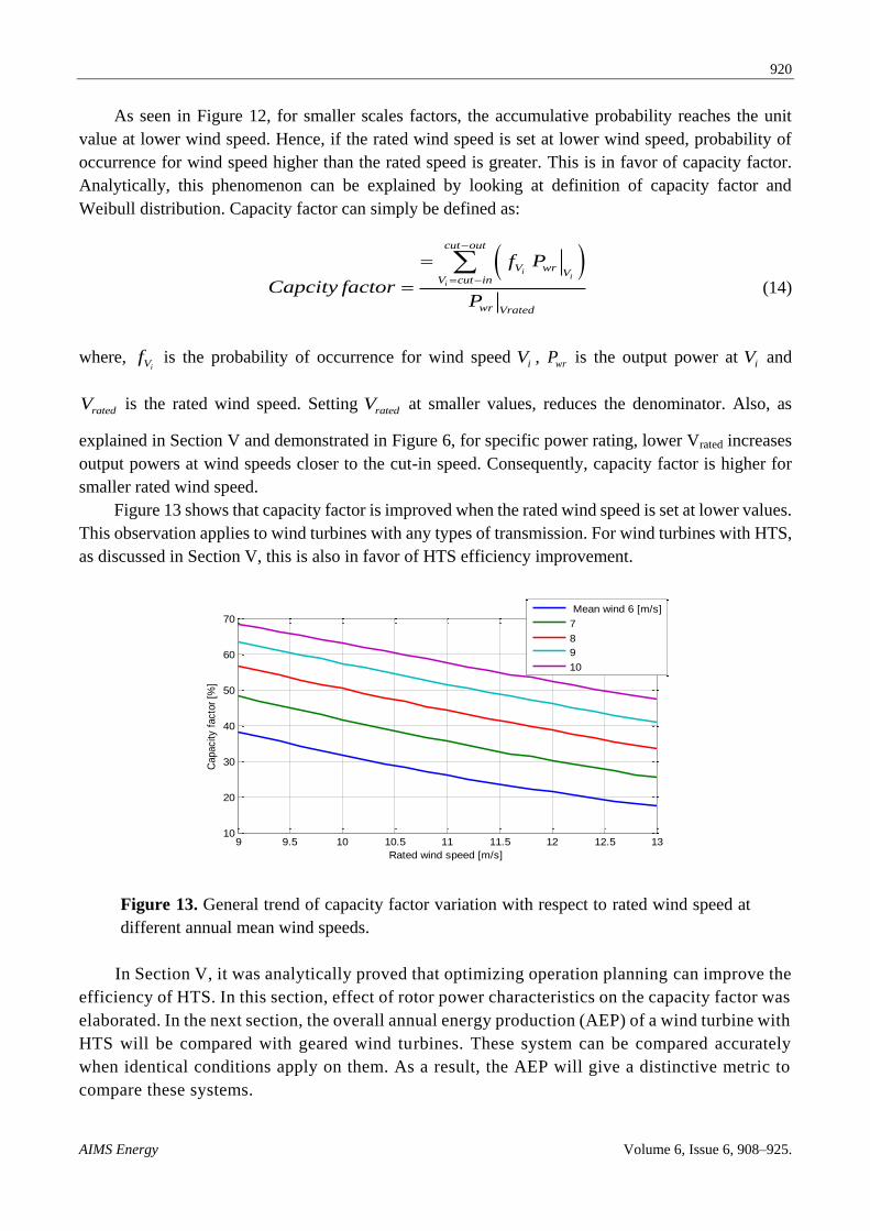
Annual mean wind speed is close to the scale factor thus in wind farms sites where the annual

mean speed is greater, higher wind speeds are experienced. In areas where experience greater annual

wind speed, setting the rated wind speed at high wind speed can yield higher energy production

annually. However, higher rated wind speed can reduce the capacity factor. This phenomenon can be

realized by looking at cumulative density function (CDF) of Weibull distribution with different scale

factors. The probability associated to each wind speed resulted from various annual mean wind speed

is shown in Figure 12.

Figure 12. Wind speed probability (CDF) at different mean wind speed for different scale

factors (shape factor 2 applied for all).

0 5 10 15 20 250

0.02

0.04

0.06

0.08

0.1

0.12

0.14

0.16

Wind speed [m/s]

Pro

babili

ty

Scale factor 6

7

8

9

10

920


As seen in Figure 12, for smaller scales factors, the accumulative probability reaches the unit

value at lower wind speed. Hence, if the rated wind speed is set at lower wind speed, probability of

occurrence for wind speed higher than the rated speed is greater. This is in favor of capacity factor.

Analytically, this phenomenon can be explained by looking at definition of capacity factor and

Weibull distribution. Capacity factor can simply be defined as:

ii

i

cut out

V wrV

V cut in

wr Vrated

f P

Capcity factorP

(14)

where, iVf is the probability of occurrence for wind speed iV , wrP is the output power at iV and

ratedV is the rated wind speed. Setting ratedV at smaller values, reduces the denominator. Also, as

explained in Section V and demonstrated in Figure 6, for specific power rating, lower Vrated increases

output powers at wind speeds closer to the cut-in speed. Consequently, capacity factor is higher for

smaller rated wind speed.

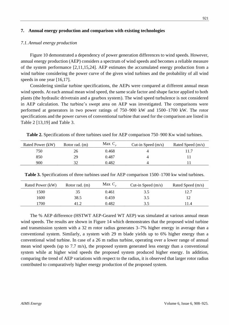
Figure 13 shows that capacity factor is improved when the rated wind speed is set at lower values.

This observation applies to wind turbines with any types of transmission. For wind turbines with HTS,

as discussed in Section V, this is also in favor of HTS efficiency improvement.

Figure 13. General trend of capacity factor variation with respect to rated wind speed at

different annual mean wind speeds.

In Section V, it was analytically proved that optimizing operation planning can improve the

efficiency of HTS. In this section, effect of rotor power characteristics on the capacity factor was

elaborated. In the next section, the overall annual energy production (AEP) of a wind turbine with

HTS will be compared with geared wind turbines. These system can be compared accurately

when identical conditions apply on them. As a result, the AEP will give a distinctive metric to

compare these systems.

9 9.5 10 10.5 11 11.5 12 12.5 1310

20

30

40

50

60

70

Rated wind speed [m/s]

Capacity f

acto

r [%

]

Mean wind 6 [m/s]

7

8

9

10

921


7. Annual energy production and comparison with existing technologies

7.1. Annual energy production

Figure 10 demonstrated a dependency of power generation differences to wind speeds. However,

annual energy production (AEP) considers a spectrum of wind speeds and becomes a reliable measure

of the system performance [2,11,15,24]. AEP estimates the accumulated energy production from a

wind turbine considering the power curve of the given wind turbines and the probability of all wind

speeds in one year [16,17].

Considering similar turbine specifications, the AEPs were compared at different annual mean

wind speeds. At each annual mean wind speed, the same scale factor and shape factor applied to both

plants (the hydraulic drivetrain and a gearbox system). The wind speed turbulence is not considered

in AEP calculation. The turbine’s swept area on AEP was investigated. The comparisons were

performed at generators in two power ratings of 750–900 kW and 1500–1700 kW. The rotor

specifications and the power curves of conventional turbine that used for the comparison are listed in

Table 2 [13,19] and Table 3.

Table 2. Specifications of three turbines used for AEP comparison 750–900 Kw wind turbines.

Rated Power (kW) Rotor rad. (m) Max pC Cut-in Speed (m/s) Rated Speed (m/s)

750 26 0.468 4 11.7

850 29 0.487 4 11

900 32 0.482 4 11

Table 3. Specifications of three turbines used for AEP comparison 1500–1700 kw wind turbines.

Rated Power (kW) Rotor rad. (m) Max pC Cut-in Speed (m/s) Rated Speed (m/s)

1500 35 0.461 3.5 12.7

1600 38.5 0.459 3.5 12

1700 41.2 0.482 3.5 11.4

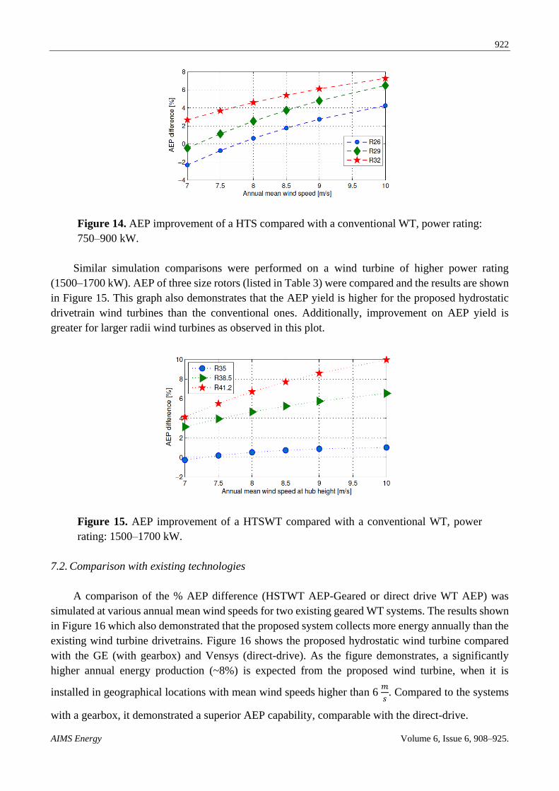
The % AEP difference (HSTWT AEP-Geared WT AEP) was simulated at various annual mean

wind speeds. The results are shown in Figure 14 which demonstrates that the proposed wind turbine

and transmission system with a 32 m rotor radius generates 3–7% higher energy in average than a

conventional system. Similarly, a system with 29 m blade yields up to 6% higher energy than a

conventional wind turbine. In case of a 26 m radius turbine, operating over a lower range of annual

mean wind speeds (up to 7.7 m/s), the proposed system generated less energy than a conventional

system while at higher wind speeds the proposed system produced higher energy. In addition,

comparing the trend of AEP variations with respect to the radius, it is observed that larger rotor radius

contributed to comparatively higher energy production of the proposed system.

922


Figure 14. AEP improvement of a HTS compared with a conventional WT, power rating:

750–900 kW.

Similar simulation comparisons were performed on a wind turbine of higher power rating

(1500–1700 kW). AEP of three size rotors (listed in Table 3) were compared and the results are shown

in Figure 15. This graph also demonstrates that the AEP yield is higher for the proposed hydrostatic

drivetrain wind turbines than the conventional ones. Additionally, improvement on AEP yield is

greater for larger radii wind turbines as observed in this plot.

Figure 15. AEP improvement of a HTSWT compared with a conventional WT, power

rating: 1500–1700 kW.

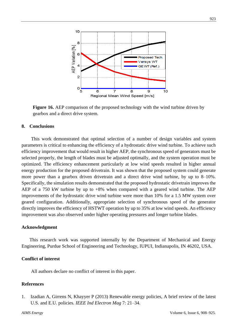
7.2. Comparison with existing technologies

A comparison of the % AEP difference (HSTWT AEP-Geared or direct drive WT AEP) was

simulated at various annual mean wind speeds for two existing geared WT systems. The results shown

in Figure 16 which also demonstrated that the proposed system collects more energy annually than the

existing wind turbine drivetrains. Figure 16 shows the proposed hydrostatic wind turbine compared

with the GE (with gearbox) and Vensys (direct-drive). As the figure demonstrates, a significantly

higher annual energy production (~8%) is expected from the proposed wind turbine, when it is

installed in geographical locations with mean wind speeds higher than 6

. Compared to the systems

with a gearbox, it demonstrated a superior AEP capability, comparable with the direct-drive.

923


Figure 16. AEP comparison of the proposed technology with the wind turbine driven by

gearbox and a direct drive system.

8. Conclusions

This work demonstrated that optimal selection of a number of design variables and system

parameters is critical to enhancing the efficiency of a hydrostatic drive wind turbine. To achieve such

efficiency improvement that would result in higher AEP, the synchronous speed of generators must be

selected properly, the length of blades must be adjusted optimally, and the system operation must be

optimized. The efficiency enhancement particularly at low wind speeds resulted in higher annual

energy production for the proposed drivetrain. It was shown that the proposed system could generate

more power than a gearbox driven drivetrain and a direct drive wind turbine, by up to 8–10%.

Specifically, the simulation results demonstrated that the proposed hydrostatic drivetrain improves the

AEP of a 750 kW turbine by up to +8% when compared with a geared wind turbine. The AEP

improvements of the hydrostatic drive wind turbine were more than 10% for a 1.5 MW system over

geared configuration. Additionally, appropriate selection of synchronous speed of the generator

directly improves the efficiency of HSTWT operation by up to 35% at low wind speeds. An efficiency

improvement was also observed under higher operating pressures and longer turbine blades.

Acknowledgment

This research work was supported internally by the Department of Mechanical and Energy

Engineering, Purdue School of Engineering and Technology, IUPUI, Indianapolis, IN 46202, USA.

Conflict of interest

All authors declare no conflict of interest in this paper.

References

1. Izadian A, Girrens N, Khayyer P (2013) Renewable energy policies, A brief review of the latest

U.S. and E.U. policies. IEEE Ind Electron Mag 7: 21–34.

924


2. Tegen S, Hand M, Maples B, et al. (2012) 2010 cost of wind energy review. No.

NREL/TP-5000-52920. National Renewable Energy Lab. (NREL), Golden, CO, United States.

3. Sheng S (2013) Report on wind turbine subsystem reliability-a survey of various databases.

NREL/PR-5000-59111. Golden, CO: National Renewable Energy Laboratory, Report.

4. Thul B, Dutta R, Stelson KA (2011) Hydrostatic transmission for mid-size wind turbines, In:

Proceedings of 52nd National Conference on Fluid Power, Las Vegas, NV, Conference

Proceedings.

5. Schmitz J, Vatheuer N, Murrenhoff H (2011) Hydrostatic drive train in wind energy plants.

RWTH Aachen University, IFAS Aachen, Germany.

6. Dutta R, Wang F, Bohlmann BF, et al. (2014) Analysis of short-term energy storage for midsize

hydrostatic wind turbine. J Dyn Syst Meas Control 136: 011007.

7. Merritt HE (1967) Hydraulic control systems. John Wiley & Sons.

8. Fitch EC (2004) Hydraulic component design and selection. Bardyne, Incorporated.

9. Manring N (2005) Hydraulic control systems. John Wiley and Sons Incorporated.

10. Bianchi FD, Battista HD, Mantz RJ (2006) Wind turbine control systems: Principles, modelling

and gain scheduling design. Springer.

11. Bhadra SN, Kastha D, Banerjee S (2005) Wind electrical systems. Oxford University Press.

12. Burton T, Jenkins N, Sharpe D, et al. (2011) Wind energy handbook. John Wiley and Sons.

13. Carrillo C, Montano AO, Cidras J, et al. (2013) Review of power curve modelling for wind

turbines. Renew Sust Energ Rev 21: 572–581.

14. Jonkman J, Butterfield S, Musial W, et al. (2009) Definition of a 5-MW reference wind turbine for

offshore system development. CO: National Renewable Energy Laboratory Golden.

15. Manwell JF, Mcgowan JG, Rogers AL (2010) Wind energy explained: Theory, design and

application. John Wiley & Sons.

16. Nielsen P, Sorsen T (2006) Windpro software user manual. Alborg, Denmark, EMD International

AS, vol. 181.

17. Johnson GL (2006) Wind energy systems. Gary L. Johnson.

18. Mon e C, Stehly T, Maples B, et al. (2015) 2014 cost of wind energy review. In: Lawrence

Berkeley National Laboratory Paper LBNL-6A20-64281.

19. West M (2005) Microsoft Excel Wind Analysis Software Program: Instructions and Walkthrough.

Available from: https://www.scribd.com/presentation/98726382/Excel-Wind-Analysis-Present.

20. Bryson AE (1975) Applied optimal control: Optimization, estimation and control. CRC Press.

21. Bertsekas DP (2005) Dynamic programming and optimal control. Athena scientific, vol. 1, no. 3.

Belmont, MA.

22. Lewis FL, Syrmos VL (1995) Optimal control. John Wiley and Sons.

23. Deldar M (2016) Decentralized multivariable modeling and control of wind turbine with

hydrostatic drivetrain. Dissertation, Purdue University.

24. Deldar M, Izadian A, Anwar S (2015) Reconfiguration of a wind turbine with hydrostatic

drivetrain to maximize annual energy production. IEEE Energ Convers Congr Expo 2015:

6660–6666.

925


25. Available from: http://mstudioblackboard.tudelft.nl/duwind/Wind%20energy%20online%20

reader/Static_pages/Cp_lamda_curve.htm.

© 2018 author name, licensee AIMS Press. This is an open access

article distributed under the terms of the Creative Commons

Attribution License (http://creativecommons.org/licenses/by/4.0)

Documents

Analysis of a hydrostatic drive wind turbine for improved