1

Analysis of Aircraft Accuracy Location in

Aeronautical Multilateration Systems

Tiago Costa

Instituto Superior Técnico / INOV-INESC

University of Lisbon

Lisbon, Portugal

tiagomrcosta@tecnico.ulisboa.pt

Abstract—Aeronautical multilateration systems enable the

locating of an aircraft based on the Time Difference of Arrival of

its signal to three or more strategically placed receiving ground

stations, located around an area of interest, providing continuous

air traffic surveillance. The aim of this dissertation was to develop

a model for the performance analysis of multilateration systems,

concerning radio coverage and aircraft location accuracy. The

proposed model considers ground stations’ location, their

antennas radiation patterns, transmitted power, receiver

sensitivity, and the corresponding parameters for the aircraft.

Line of Sight conditions are assessed by considering Digital

Elevation, Fresnel’s Ellipsoid, and the Effective Earth’s Radius

Models. The Free-Space Path Loss Model is also used, with fading

margins being set to model power oscillations due to multipath and

the aircraft orientation uncertainty. Aircraft accuracy location is

estimated from the system’s Geometric Dilution of Precision,

considering error components due to tropospheric delay,

multipath, receiver noise, quantisation, and clock bias. The model

was implemented in a simulator and successfully validated, with

results in agreement with data from the literature and previously

implemented systems. The developed model was employed in the

analysis of an implemented system from NAV Portugal, with

results suggesting that the system has a good degree of

redundancy, displaying negligible reductions in coverage, of as low

as 2%, when two out of twelve ground stations are removed. A

statistical analysis suggests that a Shifted Exponential Distribution

can model the positioning error, with parameters proportional to

the aircraft’s altitude.

Index Terms—Air Traffic Control; Distributed Positioning

Systems; Aeronautical Multilateration; Positioning Error.

I. INTRODUCTION

Aeronautical multilateration systems are used in Air Traffic Management (ATM), for the various types of airspace, allowing the extraction and display of the position and identification of an aircraft, to air traffic controllers. A reply is requested to targets within range, and the targets’ replies are captured by carefully placed Ground Stations (GS). Using a telecommunications network, the information retrieved by all the receivers is sent to a central processing unit, where targets are identified and positions are determined. Based on the Time Difference of Arrival (TDoA) of a target’s reply, to at least three GSs, it is possible to determine the target location within a confidence region.

The accuracy of this system depends on the geometry of the problem, and on the technical parameters of the target’s transponder, and the GS’s receiver; namely, their radiation patterns, transmitted power, and sensitivity. In general, the accuracy of the system is defined by the Mean Square Error (MSE) of the location. The desired capacity and separation minima between aircraft, set the minimal performance parameters of the system. The MSE of the location needs to be lower than a given threshold, to comply with these requirements.

Local Area Multilateration (LAM) systems are an essential element for Advanced Surface Movement Guidance and Control Systems (A SMGCS) in airport surveillance, allowing for the monitoring of aircraft and vehicle movements on the airport’s surface, replacing radar based systems such as the Surface Movement Radar (SMR). Contrary to radar solutions, LAM systems offer tailored coverage, combined with the ability of uniquely identifying all aircraft and vehicles on the airport surface, that are equipped with ATC transponders [1].

Wide Area Multilateration (WAM) systems are characterised by a large distance between adjacent receiver sites, otherwise known as system baseline, which can go up to 100 km, allowing for a larger coverage area than that of Secondary Surveillance Radar (SSR) and Primary Surveillance Radar (PSR) radars. The small receivers can be mounted on offshore drilling platforms, or spread over mountainous regions, offering coverage where it would be impossible to install a radar.

II. WIDE AREA MULTILATERATION

Aircraft are equipped with transponders constantly transmitting information; by exploiting these signals, measuring the TDoA of these waveforms, to receivers on the ground, it is possible to estimate the transmitter’s position. Aeronautical multilateration systems exploit the radio interface of existing technologies, such as the SSR and Automatic Dependent Surveillance-Broadcast (ADS-B) Out systems; integrating the Mode A/C/S/ES data transfer capabilities, with an independent method for locating the aircraft, and validate its reported position.

The uplink interrogation channel operates with a 1030 MHz carrier; this channel is used to interrogate cooperative aircraft in range [2]. Different modulation schemes are used, depending on the selected interrogation mode. The Mode A and C interrogations, consist of two rectangular pulses, of 0.8 μs

2

width; the separation interval between the two pulses is used by the GSs, to inform the interrogated transponders of the selected mode; for Mode A, an interval of 8 ± 0.2 μs is used; Mode C is selected with an interval of 21 ± 0.2 μs. Under these operation modes, the interrogation message is unaddressed, and all the aircraft in range, are interrogated. Mode S allows discrete interrogation of an aircraft; for this purpose, following a two-pulse preamble, an additional Differential Phased Shift Keying (DPSK) modulated data block is sent, carrying the address of the selected aircraft [2]. This mode enables a considerable reduction of interference in the channel. The transmitter power depends on the intended coverage, and is not usually disclosed by the manufacturers; nonetheless, one should expect a value that guarantees balance with the downlink.

The downlink reply channel operates at 1090 MHz , this channel is used to locate and identify cooperative aircraft in range [2]. The transponder reply message, is identical for all the operation modes, and consists of a preamble with four 0.5 μs rectangular pulses, followed by a Pulse Position Modulated (PPM) data block. The data block bitlength differs with operation mode; for modes A and C, the data block has 12 bit; and, for modes S, the data block can have 56 bit or 112 bit. The transmitter power varies between 48.5 dBm and 57 dBm , depending on the aircraft class [2].

In general, the system of TDoA equations is overdetermined; that is, at least three hyperbolic equations, associated to four receivers, are available, allowing the estimation of the three unknown aircraft coordinates. It is also possible to attain this calculation with only three receivers, through the replacement of one of the hyperboloids, by a horizontal plane [3], [4]. In this scenario, the system should get hold of the aircraft’s barometric height, as the target’s altitude defines the height of the horizontal plane; this information is usually available from a Mode C, or S, message.

Hyperbolic positioning is done over random variables; mathematically this means that the TDoA from a pair of GSs, provides not a surface, but rather a confidence region around a hyperboloid surface; therefore, the intersection of these regions gives not a single point in space, where the aircraft can be located, but rather a confidence volume. Accuracy location of aircrafts, using multilateration, becomes subject to the problem geometry; and, for every position calculation, it is required the use of GSs that minimise the position error. Regular synchronisation of the receivers’ clocks is required, to minimise the error associated with the clock offset, in each receiver; moreover, precise assessment of the positions of the GSs is key, when defining the nonlinear hyperbolic system of equations.

WAM systems are based on ToA correlation, to provide estimates for the TDoA. Using matched filter techniques, the ToAs are estimated in each sensor, and subsequently transmitted to a central processing unit. The TDoA estimator is simply the analytical difference between a pair of ToAs. This procedure is appropriate for signal waveforms where a defined pulse edge can be easily measured; as is the case with the preamble pulses in aircraft transponder signals [5], [6], [7].

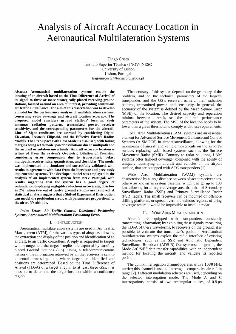
Figure 1 presents the simplified data flow for a TDoA system, based on ToA correlation.

Figure 1. Simplified data flow for a TDoA system based on ToA correlation

(adapted from [5]).

A brief description of the blocks presented in Figure 1, is provided bellow:

• Down Converter – converts the received 1090 MHz RF

signal to baseband, and allows the digitisation of the

signal;

• Digitisation – digitises the analogue signal, by means of

an appropriate Analogue-to-Digital Converter (ADC);

• ToA Measurement – calculates the ToA of the signals;

additionally, the transponder message is demodulated,

and used to identify the target;

• ToA Correlation – the ToA estimations are correlated

using the target’s identification;

• TDoA Algorithm – the correlated and grouped ToA

measurements, are applied to a TDoA algorithm, to

estimate the aircraft position;

• Tracker – improves accuracy, by filtering the raw

position data, and producing an aircraft track; this is

done by means of a tracking and filtering algorithm.

Examples of employed tracking algorithms include the

Extended Kalman Filter (EKF), the Unscented Kalman

Filter (UKF), and the Interacting Multiple Model

Kalman Filter (IMMKF) [8].

III. MODELS AND SIMULATOR DESCRIPTION

A. Model Overview

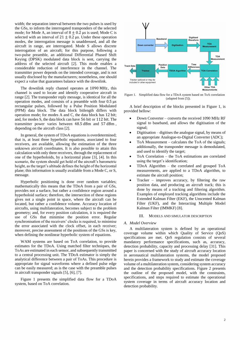
A multilateration system is defined by an operational coverage volume within which Quality of Service (QoS) specifications are met. QoS regulation consists of several mandatory performance specifications, such as, accuracy, detection probability, capacity and processing delay [31]. This paper is concerned with the study of aircraft accuracy location in aeronautical multilateration systems, the model proposed herein provides a framework to study and estimate the coverage volume of a multilateration system, considering system accuracy and the detection probability specifications. Figure 2 presents the outline of the proposed model, with the constraints, specifications, and steps required to estimate the operational system coverage in terms of aircraft accuracy location and detection probability.

3

ModelModel

Number and location of

ground stations

Design constraints

Number and location of

ground stations

Design constraints

Probability of detection

Horizontal accuracy

Performance regulations

Probability of detection

Horizontal accuracy

Performance regulations

Theoretical coverage

Theoretical accuracy

System resilience

Output

Theoretical coverage

Theoretical accuracy

System resilience

Output

Analytically determined parameters

• Expected signal-to-noise ratio

• RMS ToA error

• RMS TDoA error

• RMS positioning error

• Free-space basic transmission loss

• Fresnel ellipsoid radius

• Effective earth radius

• Orthodromic distance

• Expected signal-to-noise ratio

• RMS ToA error

• RMS TDoA error

• RMS positioning error

• Free-space basic transmission loss

• Fresnel ellipsoid radius

• Effective earth radius

• Orthodromic distance

• Expected signal-to-noise ratio

• RMS ToA error

• RMS TDoA error

• RMS positioning error

• Free-space basic transmission loss

• Fresnel ellipsoid radius

• Effective earth radius

• Orthodromic distance

Analytically determined parameters

• Expected signal-to-noise ratio

• RMS ToA error

• RMS TDoA error

• RMS positioning error

• Free-space basic transmission loss

• Fresnel ellipsoid radius

• Effective earth radius

• Orthodromic distance

Terrain profile

Antenna patterns

Receivers noise figure

Implementation

constraints

Terrain profile

Antenna patterns

Receivers noise figure

Implementation

constraints

Propagation modelling

and coverage analysis

Resilience analysis

Error modelling and

accuracy analysis

Figure 2. Model overview.

Taking a set of possible GSs’ sites, one defines the geographic volume within which the system complies with the minimum performance specifications, by discretising this volume in terms of possible aircraft coordinates, and checking, for each possible coordinate, if the minimum performance specifications are met. The flowchart of the model has 3 elementary steps, that should be run for each one of the considered aircraft coordinates:

• Coverage analysis: with a Propagation Model (PrM), and considering the minimum probability of detection specification, estimate the GSs that effectively detect the aircraft.

• Accuracy analysis: with an Error Model (ErM), and considering the minimum positioning accuracy specification, check if the aircraft coordinate is effectively covered by the system.

• Resilience analysis: considering the results from the PrM simulations, generate all the 𝑁𝐺𝑆 − 1, and 𝑁𝐺𝑆 −2 , combinations of GSs that effectively detect the aircraft, and, for each combination, reapply the ErM model to check if the aircraft coordinate is covered by the system.

The performance specifications considered for this assessment are the horizontal positioning accuracy and the detection probability. One does not consider aircraft capacity and processing delay. The developed model reduces the aircraft to a point target in an horizontal plane parallel to the Earth, disregarding the yaw, pitch and roll angles. GSs are assumed to lie on the ground within fixed and limited positions. All sensors are assumed equal, with known noise factor, sensitivity, and height Above Ground Level (AGL). Radiation patterns are assumed to be omnidirectional in the horizontal plane and with known behaviour in the vertical one; their local spherical coordinate systems are always assumed to have vertical axis normal to the Earth’s surface with the cone of silence pointing upwards for the GSs, and downwards for the aircraft. Unless otherwise specified, geographic coordinates are referenced to the 1984 World Geodetic System (WGS84) with heights referenced to the 1996 Earth Gravitational Model (EGM96) geoid.

Coverage analysis should be divided into two categories: Line-of-Sight (LoS) coverage, and sensitivity coverage. LoS coverage analysis should consider the terrain profile and the first order Fresnel ellipsoid model to determine if an aircraft and a GS are in view or if their radio-path is blocked by the terrain. On the other hand, the sensitivity coverage analysis is used to determine if the signal arriving to a receiver is above the minimum Carrier-to-Noise Ratio (CNR) threshold required to comply with the probability of detection regulation.

Accuracy analysis should be divided into three processes: the Root Mean Square (RMS) ToA error model, the RMS TDoA error model, and the RMS positioning error model. The RMS ToA error model estimates the ToA error associated with each GS-Aircraft link, considering the expected SNR and the signal bandwidth. The RMS TDoA error model measures the TDoA error associated with each of the possible GS pairs that are used to estimate the aircraft position. The RMS positioning error model takes into consideration the RMS TDoA error estimates and the geometry of the GSs network to estimate the positioning error associated with the given aircraft coordinate.

B. Error Model

A telecommunications system’s coverage is a complex concept that might depend on a number of factors, such as the received signal strength, delay between the edge of the network and its core, or capacity in terms of users and bitrate. In the case of aeronautical multilateration, coverage should also be defined in terms of aircraft location accuracy.

Considering a TDoA estimator based on ToA correlation, the RMS TDoA estimation accuracy can be modelled by a Root Sum of Squares (RSS) of the RMS ToA accuracy of each pair of sensors,

Δ𝑑𝑇𝐷𝑜𝐴 (𝐺𝑆1,𝐺𝑆2) [m] = √Δ𝑑𝑇𝑂𝐴 𝐺𝑆1 [m2]2 + Δ𝑑𝑇𝑂𝐴 𝐺𝑆2 [m2]

2 (1)

where:

• Δ𝑑𝑇𝐷𝑜𝐴 (𝐺𝑆1,𝐺𝑆2): RMS TDoA accuracy associated with

the GSs pair (𝐺𝑆1, 𝐺𝑆2),

• Δ𝑑𝑇𝑜𝐴 𝐺𝑆𝑘: RMS ToA accuracy associated with the 𝑘𝑡ℎ

GS.

Considering the several error components, the RMS ToA accuracy can be modelled by the RSS,

Δ𝑑𝑇𝑂𝐴 [m] = √∑ Δ𝑑𝒞(𝑖) [m2]2

𝑁𝒞

𝑖=1

with:

𝒞 = {𝑆𝑁𝑅; 𝑠𝑎𝑚𝑝𝑙𝑖𝑛𝑔; 𝑞𝑢𝑎𝑛𝑡𝑖𝑠𝑎𝑡𝑖𝑜𝑛; 𝑗𝑖𝑡𝑡𝑒𝑟; 𝑠𝑦𝑛𝑐}

(2)

where:

• Δ𝑑𝑆𝑁𝑅 : error component due to pulse detection

ambiguity,

• Δ𝑑𝑠𝑎𝑚𝑝𝑙𝑖𝑛𝑔 : error component due to sampling timing

ambiguity,

4

• Δ𝑑𝑞𝑢𝑎𝑛𝑡𝑖𝑠𝑎𝑡𝑖𝑜𝑛 : error component due to pulse

quantisation,

• Δ𝑑𝑗𝑖𝑡𝑡𝑒𝑟: error component due to local clock jitter,

• Δ𝑑𝑠𝑦𝑛𝑐: error component due to system synchronisation.

The effect of the additive white Gaussian noise at the matched filter detector is modelled by [61], [62],

Δ𝑑𝑆𝑁𝑅 [m] =𝑐[m s⁄ ]

2√2 𝜋 𝐵𝑤[Hz]√𝐸𝑏 [J bit⁄ ] 𝑁0 [W Hz⁄ ]⁄ (3)

where:

• Δ𝑑𝑆𝑁𝑅 : error component due to pulse detection

ambiguity,

• 𝑐: light speed in vacuum,

• 𝐵𝑤: effective bandwidth of the preamble pulses,

• 𝐸𝑏: signal energy per bit,

• 𝑁0: noise power density per Hertz of noise bandwidth.

The effect of the additive white Gaussian noise at the sampling time instant is modelled as an error component by [63],

Δ𝑑𝑠𝑎𝑚𝑝𝑙𝑖𝑛𝑔 [m] = 𝑐[m s⁄ ] Δ𝑡𝑠𝑎𝑚𝑝𝑙𝑖𝑛𝑔 [s]

√12 (4)

where:

• Δ𝑑𝑠𝑎𝑚𝑝𝑙𝑖𝑛𝑔 : error component due to sampling timing

ambiguity,

• Δ𝑡𝑠𝑎𝑚𝑝𝑙𝑖𝑛𝑔: sampling interval.

The model assumes an optimal receiver and only measures the error component due to thermal noise, corrupting the receiver’s ability to read the correct pulse time of arrival. One should complete the model with other error components, namely, the timing errors (typ. 15 m) and the propagation errors (typ. 23 m). As seen from TABLE I, the RMS ToA accuracy for each sensor is given by the RSS of several error components.

ERROR COMPONENTS OF THE RMS TOA ACCURACY

(EXTRACTED FROM [31]).

Error source Typical RMS value Reference

Timing 15 m Leeson [64]

Propagation 23 m Leeson [64]

Sensor survey 5 m Leeson [64]

Multipath Unknown Leeson [64]

AWGN Analytically determined McDonough et al. [65]

The design matrix, 𝐃, [3×𝑁𝐺𝑆], holding the aircraft-sensor geometry, has columns containing the LoS unit vectors between the aircraft and each ground station [42], [55],

𝐃[3×𝑁𝐺𝑆] = [

ρ1 𝑥 ρ𝑁𝐺𝑆 𝑥

ρ1 𝑦 ⋯ ρ𝑁𝐺𝑆 𝑦

ρ1 𝑧 ρ𝑁𝐺𝑆 𝑧

]

𝛒𝑘 [3×1] =𝐱[3×1] − 𝐱[3×1]

𝑘

‖𝐱[3×1] − 𝐱[3×1]𝑘 ‖

(5)

where:

• 𝐃: design matrix,

• 𝛒𝑘 : aircraft LoS unit vector associated with the 𝑘𝑡ℎ

ground station,

• 𝑁𝐺𝑆: number of ground stations,

• 𝐱: aircraft ECEF coordinates,

• 𝐱𝑘: 𝑘𝑡ℎ ground station ECEF coordinates.

The GDoP is a dimensionless quantity defined by the Frobenius norm [90],

𝐷𝐺𝐷𝑂𝑃 = √tr (𝐃[3×𝑁𝐺𝑆] 𝐃[𝑁𝐺𝑆×3]T ) (6)

where:

• 𝐷𝐺𝐷𝑂𝑃: Geometric Dilution of Precision,

• tr (⋅): trace of a square matrix.

The RMS position accuracy is defined as,

𝚺𝑒𝑐𝑒𝑓 [3×3][m2] = 𝐃[3×𝑁𝐺𝑆] 𝚺𝑡𝑑𝑜𝑎 [𝑁𝐺𝑆×𝑁𝐺𝑆][m2] 𝐃[𝑁𝐺𝑆×3]T (7)

where:

• 𝚺𝑒𝑐𝑒𝑓 : covariance matrix of the aircraft ECEF

positioning estimates,

• 𝚺𝑡𝑑𝑜𝑎: covariance matrix of the TDoA estimates.

Under LoS conditions the measurement errors can be considered zero-mean, independent and identically distributed Gaussian variables [66]; as a result, the covariance matrix is expressed as,

𝚺𝑡𝑑𝑜𝑎 [𝑁𝐺𝑆×𝑁𝐺𝑆][m2] = [

Δ𝑑𝑇𝐷𝑜𝐴 (𝐺𝑆1,𝐺𝑆2)2

[m]

⋮Δ𝑑𝑇𝐷𝑜𝐴 (𝐺𝑆1,𝐺𝑆𝑁𝐺𝑆

)2

[m]

] 𝐈[𝑁𝐺𝑆×𝑁𝐺𝑆] (8)

where:

• 𝐈: identity matrix.

The transformation matrix from East-North-Up (ENU) coordinates to ECEF [56],

𝐓𝑒𝑛𝑢𝑒𝑐𝑒𝑓

[3×3] = [− sin λ cos λ 0

− sin ϕ cos λ − sin ϕ sin λ cos ϕcos ϕ cos λ cos ϕ sin λ sin ϕ

] (9)

where:

• 𝐓𝑒𝑛𝑢𝑒𝑐𝑒𝑓

: coordinate transformation matrix from ENU to

ECEF coordinates.

Applying the transformation matrix, the error matrix becomes,

𝚺𝑒𝑛𝑢 [3×3][m2] = 𝐓𝑒𝑛𝑢𝑒𝑐𝑒𝑓

[3×3] 𝚺𝑒𝑐𝑒𝑓 [3×3][m2] 𝐓𝑒𝑛𝑢𝑒𝑐𝑒𝑓

[3×3]

T (10)

where:

• 𝚺𝑒𝑛𝑢: covariance matrix of the aircraft ENU positioning

estimates.

When estimating the aircraft’s position, the aeronautical service provider relies on the altitude transmitted by the on-board altimeter via ADS-B; therefore, only the East and

5

North terms of the error matrix should be considered for the accuracy analysis of the aeronautical multilateration system. In this scenario, the RMS positioning error becomes,

Δ𝑑𝑝𝑜𝑠 [m] = √Δ𝑑𝑒𝑒2

[m2] + Δ𝑑𝑛𝑛2

[m2] (11)

where:

• Δ𝑑𝑝𝑜𝑠: aircraft RMS positioning error,

• Δ𝑑𝑒𝑒2 : variance of the aircraft positioning estimates in

the East direction,

• Δ𝑑𝑛𝑛2 : variance of the aircraft positioning estimates in

the North direction.

IV. RESULTS ANALYSIS

A. Canonical scenarios

This section provides a study of the target and sensors relative positions effect on the GDoP. The target coordinates are taken from a uniform square grid of 31×31 points on the plane 𝑧 = 12.2 km (FL 400) with limits at 𝑥max = −𝑥min = 𝑦max =−𝑦min = 150 km . The sensor baseline is 100 km , a typical value for the aeronautical multilateration scenario [11].

Taking into account previous results from the literature, one expects the GDoP to display an inversely proportional trend with the number and angular distance (or apparent separation) of the sensors seen by the target [83]. Furthermore, the effect of small angular distances over the GDoP should diminish as the number of sensors increases [83].

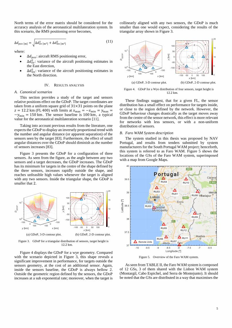
Figure 3 presents the GDoP for a configuration of three sensors. As seen from the figure, as the angle between any two sensors and a target decreases, the GDoP increases. The GDoP has its minimum for targets in the centre of the shape defined by the three sensors, increases rapidly outside the shape, and reaches unfeasible high values whenever the target is aligned with any two sensors. Inside the triangular shape, the GDoP is smaller that 2.

(a) GDoP, 3-D contour plot. (b) GDoP, 2-D contour plot.

Figure 3. GDoP for a triangular distribution of sensors, target height is

12.2 km.

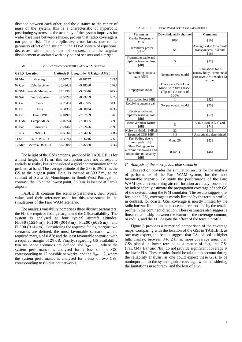
Figure 4 displays the GDoP for a wye geometry. Compared with the scenario depicted in Figure 3, this shape reveals a significant improvement in performance, for targets outside the sensors geometry, at the cost of an additional sensor. Again, inside the sensors baseline, the GDoP is always bellow 2. Outside the geometric region defined by the sensors, the GDoP increases at a sub exponential rate; moreover, when the target is

collinearly aligned with any two sensors, the GDoP is much smaller than one would expect, considering the results of the triangular array shown in Figure 3.

(a) GDoP, 3-D contour plot. (b) GDoP, 2-D contour plot.

Figure 4. GDoP for a Wye distribution of four sensors, target height is

12.2 km.

These findings suggest, that for a given FL, the sensor distribution has a small effect on performance for targets inside, or close to the region defined by the network. However, the GDoP behaviour changes drastically as the target moves away from the centre of the sensor network, this effect is more relevant for networks with less sensors, or with a non-uniform distribution of sensors.

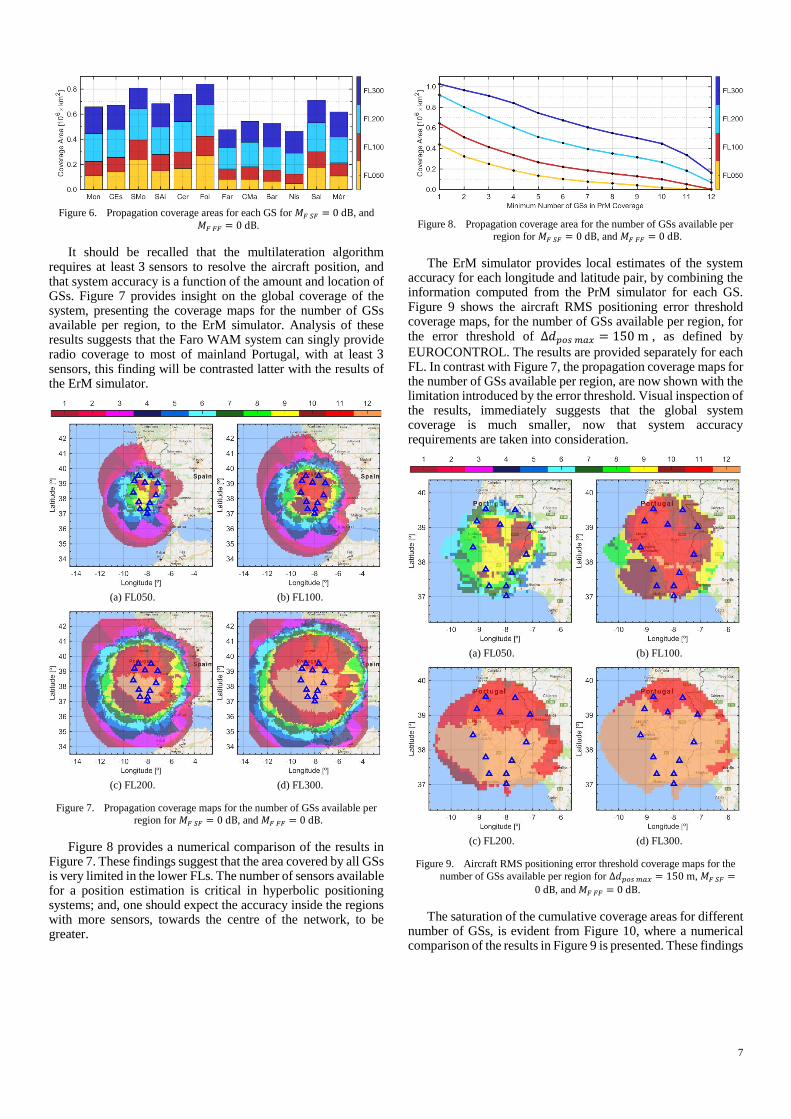
B. Faro WAM System description

The system studied in this thesis was proposed by NAV Portugal, and results from tenders submitted by system manufacturers for the South Portugal WAM project; henceforth, this system is referred to as Faro WAM. Figure 5 shows the locations of the GSs of the Faro WAM system, superimposed with a map from Google Maps.

Figure 5. Overview of the Faro WAM system.

As seen from TABLE II, the Faro WAM system is composed of 12 GSs, 3 of them shared with the Lisbon WAM system (Montargil, Cabo Espichel, and Serra de Montejunto). It should be noted that the GSs are distributed in a way that maximises the

6

distance between each other, and the distance to the centre of mass of the system, this is a characteristic of hyperbolic positioning systems, as the accuracy of the system improves for wider baselines between sensors, proven that radio coverage is not put at risk. The multiplicative error factor, due to the geometry effect of the system in the TDoA system of equations, decreases with the number of sensors, and the angular displacement associated with any pair of sensors and a target.

GROUND STATIONS OF THE FARO WAM SYSTEM.

GS ID Location Latitude [º] Longitude [º] Height AMSL [m]

01 Mon Montargil 39.07725 -8.18757 243.7

02 CEs Cabo Espichel 38.42431 -9.18590 176.7

03 SMo Serra de Montejunto 39.17386 -9.05346 675.2

04 SAi Serra de Aire 39.53205 -8.73209 567.2

05 Cer Cercal 37.79451 -8.71825 343.9

06 Foi Foia 37.31357 -8.60024 893.2

07 Far Faro TWR 37.01907 -7.97109 26.0

08 CMa Campo Maior 39.02724 -7.08595 339.8

09 Bar Barrancos 38.21448 -7.22676 239.3

10 Nis Nisa RT 39.50340 -7.64286 308.2

11 Sal Salir DME RT 37.30761 -7.96246 586.9

12 Mér Mértola DME RT 37.70088 -7.76380 353.7

The height of the GS’s antenna, provided in TABLE II, is for a mast height of 12 m, this assumption does not correspond entirely to reality but is considered a good approximation for the problem at hand. The average altitude of the GSs is 396.2 m, the GS at the highest point, Foia, is located at 893.2 m , at the summit of Serra de Monchique, in South-West Portugal; in contrast, the GS at the lowest point, 26.0 m, is located at Faro’s airport.

TABLE III contains the scenario parameters, their typical value, and their reference used for this assessment in the simulations of the Faro WAM scenario.

The analysis variability comprises three distinct parameters, the FL, the required fading margin, and the GSs availability. The system is analysed at four typical aircraft altitudes, FL050 (1524 m) , FL100 (3048 m) , FL200 (6096 m) , and FL300 (9144 m). Considering the required fading margins two scenarios are defined, the most favourable scenario, with a required margin of 0 dB; and the least favourable scenario, with a required margin of 29 dB. Finally, regarding GS availability two resilience scenarios are defined, the 𝑁𝐺𝑆 − 1 , where the system performance is analysed for a loss of one GS, corresponding to 12 possible networks; and the 𝑁𝐺𝑆 − 2, where the system performance is analysed for a loss of two GSs, corresponding to 66 distinct networks.

FARO WAM SCENARIO PARAMETERS.

Parameter Downlink reply channel Comment

Carrier Frequency

[MHz] 1090 [16]

Transmitter power

[dBm] 54

Average value for aircraft transponders, [85] and

[16]

Transmitter cable and

diplexer insertion loss

[dB] 3 [52]

Transmitting antenna

gain [dBi] Nonparametric model

Simulations for a narrow-body, commercial

passenger, twin-engine jet

airliner

Propagation model

Free-Space Path Loss

Model with first Fresnel

ellipsoid clearance of

100%

-

Polarisation loss [dB] 1 [52]

Receiving antenna gain

[dBi] Nonparametric model [75]

Receiver cable and

diplexer insertion loss

[dB] 1 [52]

Receiver noise factor

[dB] 5

Value used in [73] and [74]

Noise bandwidth [MHz] 22 [11]

Required CNR [dB] 6.3 Analytically determined

Fast Fading due to

multipath [dB] 0 and 26 [52]

Slow Fading due to

airframe shadowing and orientation uncertainty

[dB]

0 and 3 [46]

C. Analysis of the most favourable scenario

This section provides the simulation results for the analysis of performance of the Faro WAM system, for the most favourable scenario. To study the performance of the Faro WAM system concerning aircraft location accuracy, one starts by independently estimate the propagation coverage of each GS of the system, using the PrM simulator. The results suggest that for inland GSs, coverage is mostly limited by the terrain profile; in contrast, for coastal GSs, coverage is mostly limited by the radio horizon limitation in the ocean direction, and by the terrain profile in the continent direction. These estimates also suggest a linear relationship between the extent of the coverage contour, or radius, and the FL, despite the effect of the terrain profile.

Figure 6 provides a numerical comparison of the coverage maps. Comparing with the location of the GSs in TABLE II, as one may expect, the results suggest that GSs placed in higher hills display, between 3 to 2 times more coverage area, than GSs placed in lower terrain; as a matter of fact, the GSs {Far, CMa, Bar and Nis} do not provide significant coverage at the lower FLs. These results should be taken into account during the reliability analysis, as one could expect these GSs, to be nonimportant to the system global coverage, when considering the limitations in accuracy, and the loss of a GS.

7

Figure 6. Propagation coverage areas for each GS for 𝑀𝐹 𝑆𝐹 = 0 dB, and

𝑀𝐹 𝐹𝐹 = 0 dB.

It should be recalled that the multilateration algorithm requires at least 3 sensors to resolve the aircraft position, and that system accuracy is a function of the amount and location of GSs. Figure 7 provides insight on the global coverage of the system, presenting the coverage maps for the number of GSs available per region, to the ErM simulator. Analysis of these results suggests that the Faro WAM system can singly provide radio coverage to most of mainland Portugal, with at least 3 sensors, this finding will be contrasted latter with the results of the ErM simulator.

(a) FL050. (b) FL100.

(c) FL200. (d) FL300.

Figure 7. Propagation coverage maps for the number of GSs available per

region for 𝑀𝐹 𝑆𝐹 = 0 dB, and 𝑀𝐹 𝐹𝐹 = 0 dB.

Figure 8 provides a numerical comparison of the results in Figure 7. These findings suggest that the area covered by all GSs is very limited in the lower FLs. The number of sensors available for a position estimation is critical in hyperbolic positioning systems; and, one should expect the accuracy inside the regions with more sensors, towards the centre of the network, to be greater.

Figure 8. Propagation coverage area for the number of GSs available per

region for 𝑀𝐹 𝑆𝐹 = 0 dB, and 𝑀𝐹 𝐹𝐹 = 0 dB.

The ErM simulator provides local estimates of the system accuracy for each longitude and latitude pair, by combining the information computed from the PrM simulator for each GS. Figure 9 shows the aircraft RMS positioning error threshold coverage maps, for the number of GSs available per region, for the error threshold of Δ𝑑𝑝𝑜𝑠 𝑚𝑎𝑥 = 150 m , as defined by

EUROCONTROL. The results are provided separately for each FL. In contrast with Figure 7, the propagation coverage maps for the number of GSs available per region, are now shown with the limitation introduced by the error threshold. Visual inspection of the results, immediately suggests that the global system coverage is much smaller, now that system accuracy requirements are taken into consideration.

(a) FL050. (b) FL100.

(c) FL200. (d) FL300.

Figure 9. Aircraft RMS positioning error threshold coverage maps for the

number of GSs available per region for Δ𝑑𝑝𝑜𝑠 𝑚𝑎𝑥 = 150 m, 𝑀𝐹 𝑆𝐹 =

0 dB, and 𝑀𝐹 𝐹𝐹 = 0 dB.

The saturation of the cumulative coverage areas for different number of GSs, is evident from Figure 10, where a numerical comparison of the results in Figure 9 is presented. These findings

8

suggest that for the higher FLs, accuracy is not limited by the number of GSs; instead, accuracy appears to be limited by the geometry of the system; in other words, the limiting factor is the narrowing of the apparent angle between the aircraft and any pair of sensors, as it moves away from the centre of the system. Moreover, one may expect that removing a sensor in these conditions does not affect performance. Figure 11 provides the spatial distribution of the positioning error. The positioning error has its lower values inside the region delimited by the GSs; with a guaranteed maximum RMS positioning error of 50 m, for all FLs.

The positioning error was computed for every longitude and latitude sample, with at least three corresponding GSs available; as seen previously in Figure 7, this region corresponds to the area painted in light magenta. In what follows, is provided the statistical analysis for the spatial distribution of the positioning error inside this region. In Figure 12 an histogram for each FL is presented with the corresponding proposed theoretical model for the population. The histograms suggest a saturation of the positioning error towards the minimum value, this result is also confirmed by inspection of the raw positioning error values. The histograms are plotted with the shifted exponential distribution fitted by maximum likelihood estimation for the observations at each FL.

The proposed theoretical distribution overestimates the positioning error, failing to correctly model the saturation around the minimum. Nonetheless, the shifted exponential distribution is suggested as a model for the spatial behaviour of the positioning error population, exhibiting the best ratio between model goodness-of-fit, model complexity, and explanatory power. Due to the significant increase in coverage with FL, the number of longitude and latitude samples is much higher for higher FLs, this expansion of the region considered for error analysis, matched with a decrease in the angular displacement between any pair of GSs and a sample, causes the tails of the empirical distribution to grow in length with higher FLs.

Figure 10. Aircraft RMS positioning error threshold coverage area for the

number of GSs available per region for Δ𝑑𝑝𝑜𝑠 𝑚𝑎𝑥 = 150 m, 𝑀𝐹 𝑆𝐹 =

0 dB, and 𝑀𝐹 𝐹𝐹 = 0 dB.

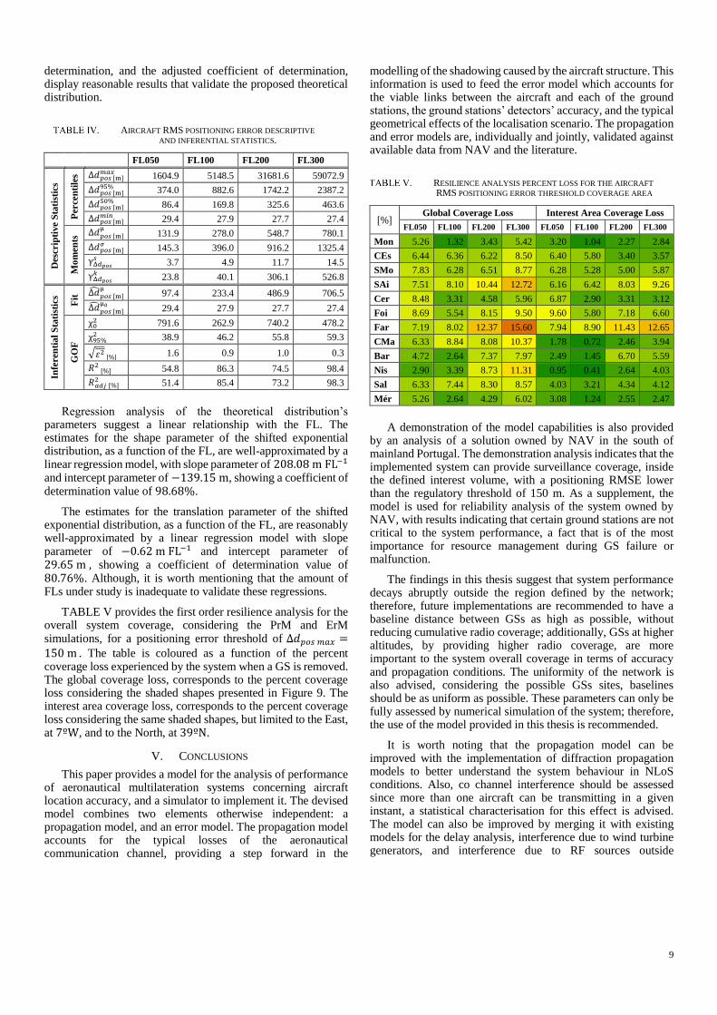
TABLE IV provides the descriptive and inferential statistics for the results in Figure 11. The descriptive statistics display a linear relationship with FL. It is worth mentioning that all statistics but the minimum positioning error, increase with increasing FL. The growth with FL of the region covered by at least 12 GSs might suggest an explanation for the slightly decrease with FL of the minimum value observed for the positioning error dataset.

(a) FL050. (b) FL100.

(c) FL200. (d) FL300.

Figure 11. Aircraft RMS positioning error spatial distribution for 𝑀𝐹 𝑆𝐹 =0 dB, and 𝑀𝐹 𝐹𝐹 = 0 dB.

(a) FL050. (b) FL100.

(c) FL200. (d) FL300.

Figure 12. Aircraft RMS positioning error histogram and fitted distribution

for 𝑀𝐹 𝑆𝐹 = 0 dB, and 𝑀𝐹 𝐹𝐹 = 0 dB.

The results for the inference on the positioning error population are also presented in TABLE IV; the chi-squared goodness-of-fit test rejects the hypothesis that the data is consistent with the shifted exponential distribution, this result is explained by the inability of the theoretical distribution to model the saturated observations about the minimum, and the sensitivity of the chi-squared goodness-of-fit test to outliers. Alternative metrics, such as the RMSE, the coefficient of

9

determination, and the adjusted coefficient of determination, display reasonable results that validate the proposed theoretical distribution.

AIRCRAFT RMS POSITIONING ERROR DESCRIPTIVE AND INFERENTIAL STATISTICS.

FL050 FL100 FL200 FL300

Desc

rip

tive S

tati

stic

s

Perce

nti

les Δ𝑑𝑝𝑜𝑠 [m]

𝑚𝑎𝑥 1604.9 5148.5 31681.6 59072.9

Δ𝑑𝑝𝑜𝑠 [m]95% 374.0 882.6 1742.2 2387.2

Δ𝑑𝑝𝑜𝑠 [m]50% 86.4 169.8 325.6 463.6

Δ𝑑𝑝𝑜𝑠 [m]𝑚𝑖𝑛 29.4 27.9 27.7 27.4

Mo

men

ts Δ𝑑𝑝𝑜𝑠 [m]

µ 131.9 278.0 548.7 780.1

Δ𝑑𝑝𝑜𝑠 [m]𝜎 145.3 396.0 916.2 1325.4

γΔ𝑑𝑝𝑜𝑠

𝑠 3.7 4.9 11.7 14.5

γΔ𝑑𝑝𝑜𝑠

𝑘 23.8 40.1 306.1 526.8

Infe

ren

tia

l S

tati

stic

s

Fit

Δ�̂�𝑝𝑜𝑠 [m]µ

97.4 233.4 486.9 706.5

Δ�̂�𝑝𝑜𝑠 [m]µ0 29.4 27.9 27.7 27.4

GO

F

χ02 791.6 262.9 740.2 478.2

χ95%2 38.9 46.2 55.8 59.3

√𝜀2̅̅̅ [%] 1.6 0.9 1.0 0.3

𝑅2 [%] 54.8 86.3 74.5 98.4

𝑅𝑎𝑑𝑗2

[%] 51.4 85.4 73.2 98.3

Regression analysis of the theoretical distribution’s parameters suggest a linear relationship with the FL. The estimates for the shape parameter of the shifted exponential distribution, as a function of the FL, are well-approximated by a linear regression model, with slope parameter of 208.08 m FL−1 and intercept parameter of −139.15 m, showing a coefficient of determination value of 98.68%.

The estimates for the translation parameter of the shifted exponential distribution, as a function of the FL, are reasonably well-approximated by a linear regression model with slope parameter of −0.62 m FL−1 and intercept parameter of 29.65 m , showing a coefficient of determination value of 80.76%. Although, it is worth mentioning that the amount of FLs under study is inadequate to validate these regressions.

TABLE V provides the first order resilience analysis for the overall system coverage, considering the PrM and ErM simulations, for a positioning error threshold of Δ𝑑𝑝𝑜𝑠 𝑚𝑎𝑥 =150 m . The table is coloured as a function of the percent coverage loss experienced by the system when a GS is removed. The global coverage loss, corresponds to the percent coverage loss considering the shaded shapes presented in Figure 9. The interest area coverage loss, corresponds to the percent coverage loss considering the same shaded shapes, but limited to the East, at 7ºW, and to the North, at 39ºN.

V. CONCLUSIONS

This paper provides a model for the analysis of performance of aeronautical multilateration systems concerning aircraft location accuracy, and a simulator to implement it. The devised model combines two elements otherwise independent: a propagation model, and an error model. The propagation model accounts for the typical losses of the aeronautical communication channel, providing a step forward in the

modelling of the shadowing caused by the aircraft structure. This information is used to feed the error model which accounts for the viable links between the aircraft and each of the ground stations, the ground stations’ detectors’ accuracy, and the typical geometrical effects of the localisation scenario. The propagation and error models are, individually and jointly, validated against available data from NAV and the literature.

RESILIENCE ANALYSIS PERCENT LOSS FOR THE AIRCRAFT RMS POSITIONING ERROR THRESHOLD COVERAGE AREA

[%] Global Coverage Loss Interest Area Coverage Loss

FL050 FL100 FL200 FL300 FL050 FL100 FL200 FL300

Mon 5.26 1.32 3.43 5.42 3.20 1.04 2.27 2.84

CEs 6.44 6.36 6.22 8.50 6.40 5.80 3.40 3.57

SMo 7.83 6.28 6.51 8.77 6.28 5.28 5.00 5.87

SAi 7.51 8.10 10.44 12.72 6.16 6.42 8.03 9.26

Cer 8.48 3.31 4.58 5.96 6.87 2.90 3.31 3.12

Foi 8.69 5.54 8.15 9.50 9.60 5.80 7.18 6.60

Far 7.19 8.02 12.37 15.60 7.94 8.90 11.43 12.65

CMa 6.33 8.84 8.08 10.37 1.78 0.72 2.46 3.94

Bar 4.72 2.64 7.37 7.97 2.49 1.45 6.70 5.59

Nis 2.90 3.39 8.73 11.31 0.95 0.41 2.64 4.03

Sal 6.33 7.44 8.30 8.57 4.03 3.21 4.34 4.12

Mér 5.26 2.64 4.29 6.02 3.08 1.24 2.55 2.47

A demonstration of the model capabilities is also provided by an analysis of a solution owned by NAV in the south of mainland Portugal. The demonstration analysis indicates that the implemented system can provide surveillance coverage, inside the defined interest volume, with a positioning RMSE lower than the regulatory threshold of 150 m. As a supplement, the model is used for reliability analysis of the system owned by NAV, with results indicating that certain ground stations are not critical to the system performance, a fact that is of the most importance for resource management during GS failure or malfunction.

The findings in this thesis suggest that system performance decays abruptly outside the region defined by the network; therefore, future implementations are recommended to have a baseline distance between GSs as high as possible, without reducing cumulative radio coverage; additionally, GSs at higher altitudes, by providing higher radio coverage, are more important to the system overall coverage in terms of accuracy and propagation conditions. The uniformity of the network is also advised, considering the possible GSs sites, baselines should be as uniform as possible. These parameters can only be fully assessed by numerical simulation of the system; therefore, the use of the model provided in this thesis is recommended.

It is worth noting that the propagation model can be improved with the implementation of diffraction propagation models to better understand the system behaviour in NLoS conditions. Also, co channel interference should be assessed since more than one aircraft can be transmitting in a given instant, a statistical characterisation for this effect is advised. The model can also be improved by merging it with existing models for the delay analysis, interference due to wind turbine generators, and interference due to RF sources outside

10

aeronautical telecommunications. The simulator can be programmed to be a general-purpose tool for the assessment of the aeronautical Communication, Navigation, and Surveillance (CNS) infrastructure since much of the geometry, propagation and error algorithms are already implemented. The model for the error component due to noise and signal bandwidth in the ToA estimation is shared with many other systems such as the PSR, the SSR, and Navigational Aid (NAVAID) technologies such as the Distance Measuring Equipment (DME). The model for the GDoP can also be adapted to assess accuracy in emergent surveillance systems, such as the Multi-Static Primary Surveillance Radar (MSPSR).

ACKNOWLEDGMENT

I would like to express my sincere gratitude to my thesis supervisor, Prof. Luís M. Correia, for all the knowledge, guidance, motivation, consideration, and time, shared with me during the development of this work.

I would also very much like to thank NAV Portugal; particularly, Eng. Carlos Alves, Eng. André Maia, and Eng. Luís Pissarro, whose valuable input and feedback were paramount to the development, improvement, and technical relevance of this work.

REFERENCES

[1] Era Systems Corporation, Multilateration - Executive Reference Guide, Era Systems Corporation, Pardubice, Czech Republic, (http://www.multilateration.com/downloads/MLAT-ADS-B-Reference-Guide.pdf).

[2] ICAO, Annex 10 — Aeronautical Telecommunications: Volume IV — Surveillance and Collision Avoidance Systems, 5th Edition, International Standards and Recommended Practices, ICAO, Montréal, Quebec, Canada, Jul. 2014.

[3] K. Pourvoyeur, A. Mathias, and R. Heidger, “Investigation of Measurement Characteristics of MLAT / WAM and ADS-B,” in Proc. of TIWDC/ESAV’11 - 22nd IEEE Tyrrhenian International Workshop on Digital Communications - Enhanced Surveillance of Aircraft and Vehicles, Capri, Italy, Sep. 2011 (http://ieeexplore.ieee.org/stamp/stamp.jsp?tp=&arnumber=6060989).

[4] N. Xu, R. Cassell, C. Evers, S. Hauswald, and W. Langhans, “Performance assessment of Multilateration Systems - a solution to nextgen surveillance,” in Proc. of ICNS’10 - 10th IEEE Integrated Communications, Navigation and Surveilance Conference, Herndon, VA, USA, May 2010 (http://ieeexplore.ieee.org/stamp/stamp.jsp?tp=&arnumber=5503290).

[5] W.H.L. Neven, T.J. Quilter, R. Weedon, and R.A. Hogendoorn, Report on Wide Area Multilateration, Report on EATMP TRS 131/04, Deliverable NLR-CR-2004-472, EUROCONTROL, Brussels, Belgium, Aug. 2005 (https://www.eurocontrol.int/sites/default/files/publication/files/surveilllance-report-wide-area-multilateration-200508.pdf).

[6] S. Gezici and H.V. Poor, “Position Estimation via Ultra-Wideband Signals,” Proceedings of the IEEE - Special Issue on UWB Technology and Emerging Applications, Vol. 97, No. 2, Feb. 2009, pp. 386–403 (http://ieeexplore.ieee.org/lpdocs/epic03/wrapper.htm?arnumber=4796279).

[7] H.I. Ahmed, P. Wei, I. Memon, Y. Du, and W. Xie, “Estimation of Time Difference of Arrival (TDOA) for the Source Radiates BPSK Signal,” International Journal of Computer Science Issues (IJCSI), Vol. 10, No. 3, May 2013, pp. 164–171 (http://ijcsi.org/papers/IJCSI-10-3-2-164-171.pdf).

[8] R.A. Hogendoorn, C. Rekkas, and W.H.L. Neven, “ARTAS: An IMM-based Multisensor Tracker,” in Proc. of FUSION’99 - 2nd IEEE International Conference on Information Fusion, Sunnyvale, CA, USA, Jul. 1999 (http://fusion.isif.org/proceedings/fusion99CD/C-131.pdf?).