Embed Size (px)
Citation preview
Analysis of Pile-Concrete Connectionsin Near-Shore Applications
S. Belfroid
Mas
ter
ofSc
ienc
eT
hesi
s

Analysis of Pile-Concrete Connections in
Near-Shore Applications
In partial fulfilment of the requirements for the degree of
Master of Science
In Civil Engineering at Delft University of Technology
by
S. Belfroid
September 2015
Thesis Committee:
Prof. ir. F.S.K. Bijlaard TU Delft, Steel Constructions (Chairman)
Ir. R. Abspoel TU Delft, Steel Constructions
Dr. ir. drs. C.R. Braam TU Delft, Concrete Structures
Dr. ir. M.A.N. Hendriks TU Delft, Structural Mechanics
Ing. F. van der Woerdt MBA Ballast Nedam Engineering
An electronic version of this thesis is available at http://repository.tudelft.nl/.
Faculty of Civil Engineering and Geosciences (CiTG)
Delft University of Technology

i
Summary
Tubular steel sections are used as foundation piles in near-shore applications like jetties or
bridgeworks. The steel tubes are connected to a concrete capping beam or pile cap which transfers the
forces from the structure to the piles. Multiple options for this connection type have been developed
over the years with varying specifications. Constructability, costs and construction time are of high
importance when adopting an alternative.
The possible options have been identified by means of a literature survey. These alternatives follow
from various disciplines like pile-footing, pile-to-cap and concrete filled tubes (CFT). Design issues or
problems are acknowledged and a consideration is made about the applicability. A further distinction
is made by introducing the trade-off aspects like the costs, the construction time and the
manufacturability.
The concrete plug connection seems the most used and suitable option. Only in a few situations, this
connection is not applicable. A major design problem is the relatively unknown bond strength between
the concrete plug and the steel pile. This bond stress is examined in more detail and most influences
are identified. Current design expressions, including pile-sleeve formulations, are elaborated by a
comparative study in relation to the influences on bond strength found in testing. Furthermore, a new
analytical model for the bond strength for circular tubes is proposed. Based on the stresses and strains
of both the steel and the concrete, this formulation is obtained by solving the equations. This newly
derived formulation (DF) is verified using 61 selected test specimens with the appropriate failure
mechanism. When comparing the outcome of this analysis with other bond expressions, the new
formulation results in the largest prediction for the 61 specimens with the lowest standard deviation. In
combination with the correction factor, this formula calculates safely the bond capacity between the
steel pile and the concrete core.
The model is expanded to allow for shear keys in the connection. Unfortunately, this expression
cannot be verified as in the case of the bond capacity due to the lack of experimental data. Lastly, a
proposition is done for the bending moment capacity of the connection. Two major assumptions in this
model need to be verified with testing.
Summary
ii
iii
Preface & Acknowledgements
This document is the Master’s thesis report to finalize the Master Structural Engineering at Delft
University of Technology. This document is established in cooperation with Ballast Nedam
Engineering. I first came in contact with Ballast Nedam Engineering on the company fair at the civil
engineering faculty. I had a very interesting talk with one of the employees about internships and
graduation projects. Infected with enthusiasm, I contacted the engineering department for an
appointment.
During the first interview, an idea arose for the graduation topic: the connection between steel piles
and concrete elements in near-shore applications. What intrigued me the most concerning this topic is
the interface between the steel and the concrete. Multiple disciplines are involved which results in
great and numerous difficulties. Right after a very interesting conversation with the professor, I
accepted the challenge.
I am really grateful for the opportunity that I got at Ballast Nedam Engineering. Special thanks go to
my supervisor Frank van der Woerdt. I want to thank you for the inspiring meetings we had and for
the wisdom you provided. Furthermore, I want to thank all members of the committee for guiding me
through this process. I found the consultations very interesting and inspirational.
Of course, I want to thank my parents, family and friends for the support. Not only during completion
of this thesis but also during the rest of my study and beyond. Mam, pap, de laatste is dan ook
eindelijk afgeleverd. Ik kan jullie niet genoeg bedanken voor alles wat jullie voor mij hebben gedaan.
Anne-Michelle, thanks for all the support during completion of this work. You could always get my
mind off when I needed it. I could not thank you enough.
Delft, University of Technology,
September 2015
Bas Belfroid
Preface & Acknowledgements
iv
v
Contents
1. Problem Description ....................................................................................................................... 1
Motivation .................................................................................................................................. 1 1.1
Research objectives .................................................................................................................... 1 1.2
Outline ........................................................................................................................................ 2 1.3
2. Applications & Background ........................................................................................................... 3
Applications ................................................................................................................................ 3 2.1
2.1.1 Force deviation ................................................................................................................... 4
2.1.2 Loading .............................................................................................................................. 5
Pipe piles .................................................................................................................................... 5 2.2
2.2.1 Production methods ............................................................................................................ 6
2.2.2 Driving tolerances .............................................................................................................. 6
2.2.3 Corrosion ............................................................................................................................ 7
2.2.4 Capacity ............................................................................................................................. 7
Capping beam/pile cap ............................................................................................................... 8 2.3
2.3.1 Reinforcement design......................................................................................................... 8
Conclusion .................................................................................................................................. 9 2.4
3. Alternatives ................................................................................................................................... 11
Design strategies ....................................................................................................................... 11 3.1
3.1.1 Seismic design strategy .................................................................................................... 11
3.1.2 Non-seismic design strategy ............................................................................................ 12
Connection alternatives ............................................................................................................ 12 3.2
3.2.1 In-situ capping beam/pile cap .......................................................................................... 12
3.2.2 Prefab capping beam/pile cap .......................................................................................... 14
3.2.3 Both prefab and in-situ ..................................................................................................... 16
Suitability for seismic regions .................................................................................................. 19 3.3
Conclusion ................................................................................................................................ 19 3.4
4. Decision Model............................................................................................................................. 21
Design influences ..................................................................................................................... 21 4.1
4.1.1 Aspect groups ................................................................................................................... 21
Advanced decisions .................................................................................................................. 21 4.2
Decision scheme ....................................................................................................................... 22 4.3
4.3.1 Instructions ....................................................................................................................... 22
Contents
vi
4.3.2 Demonstrations ................................................................................................................ 22
4.3.3 Appearance....................................................................................................................... 23
Trade-off ................................................................................................................................... 23 4.4
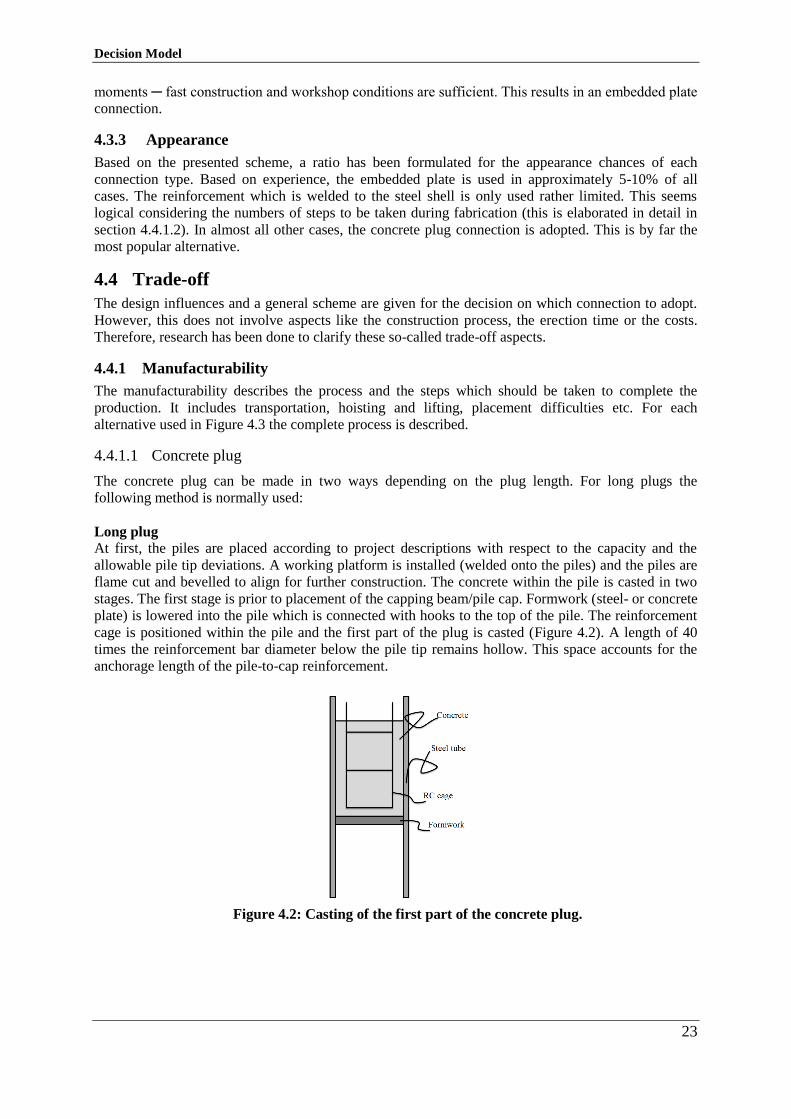
4.4.1 Manufacturability ............................................................................................................. 23
4.4.2 Durability ......................................................................................................................... 28
4.4.3 Construction time ............................................................................................................. 29
4.4.4 Costs analysis ................................................................................................................... 30
Conclusion ................................................................................................................................ 31 4.5
5. Behaviour Plug Connection .......................................................................................................... 33
Axial behaviour without shear keys ......................................................................................... 33 5.1
5.1.1 Pull-out ............................................................................................................................. 33
5.1.2 Push-out ........................................................................................................................... 35
5.1.3 Design capacity ................................................................................................................ 35
Axial behaviour with shear keys .............................................................................................. 35 5.2
5.2.1 Pile-sleeve systems .......................................................................................................... 36
Bending moment and shear behaviour ..................................................................................... 37 5.3
Conclusion ................................................................................................................................ 37 5.4
6. Axial Capacity Without Shear Keys ............................................................................................. 39
Bond ......................................................................................................................................... 39 6.1
Parameter study ........................................................................................................................ 40 6.2
6.2.1 Concrete compressive strength ........................................................................................ 40
6.2.2 Interface length/diameter ................................................................................................. 41
6.2.3 Pipe pile diameter ............................................................................................................. 41
6.2.4 Shrinkage ......................................................................................................................... 42
6.2.5 Compaction of the concrete ............................................................................................. 43
6.2.6 Surface roughness ............................................................................................................ 43
6.2.7 Eccentric loading .............................................................................................................. 43
6.2.8 Cyclic loading .................................................................................................................. 43
Improvement ............................................................................................................................ 45 6.3
6.3.1 Fly ash .............................................................................................................................. 45
Bond stress along the interface ................................................................................................. 45 6.4
Design expressions ................................................................................................................... 46 6.5
6.5.1 Circular piles .................................................................................................................... 46
6.5.2 Roeder et al. (1999). ......................................................................................................... 46
6.5.3 Pile-sleeve systems .......................................................................................................... 46
6.5.4 Comparison (example) ..................................................................................................... 48
Conclusion ................................................................................................................................ 49 6.6
7. New Axial Strength Model Without Shear Keys .......................................................................... 51
Definitions ................................................................................................................................ 51 7.1
Contents
vii
Friction ..................................................................................................................................... 52 7.2
Steel stresses and strain ............................................................................................................ 53 7.3
7.3.1 Thin walled cylinders ....................................................................................................... 53
7.3.2 Circumferential stress....................................................................................................... 53
7.3.3 Longitudinal stress ........................................................................................................... 54
7.3.4 Radial stress ..................................................................................................................... 54
7.3.5 Circumferential strain....................................................................................................... 54
Concrete stresses and strain ...................................................................................................... 55 7.4
7.4.1 Circumferential and radial stress ...................................................................................... 55
7.4.2 Longitudinal stress ........................................................................................................... 56
7.4.3 Concrete strain ................................................................................................................. 56
Relative displacement between pile and plug ........................................................................... 56 7.5
Bond expression ....................................................................................................................... 57 7.6
Stiffness factor K ...................................................................................................................... 57 7.7
7.7.1 Comparing stiffness factors .............................................................................................. 58
Bond formulation ..................................................................................................................... 58 7.8
Final bond formulation including shrinkage ............................................................................ 58 7.9
Assumptions ......................................................................................................................... 59 7.10
Conclusion ............................................................................................................................ 60 7.11
8. Comparison Bond Formulation to Test Results ............................................................................ 61
Comparing trends ..................................................................................................................... 61 8.1
8.1.1 Interface length ................................................................................................................ 61
8.1.2 Diameter ........................................................................................................................... 62
8.1.3 Thickness ......................................................................................................................... 63
8.1.4 Concrete compressive strength ........................................................................................ 63
8.1.5 Difference pull- and push-out .......................................................................................... 64
Shrinkage models ..................................................................................................................... 64 8.2
8.2.1 Models .............................................................................................................................. 65
Matching to test results ............................................................................................................. 66 8.3
8.3.1 Validation ......................................................................................................................... 67
8.3.2 Comparison of theoretical and experimental values ........................................................ 67
8.3.3 Correction......................................................................................................................... 68
8.3.4 Comparison with correction factor ................................................................................... 69
Comparison with other expressions .......................................................................................... 69 8.4
8.4.1 Design factors .................................................................................................................. 70
8.4.2 Comparison of the different shrinkage models ................................................................ 70
Conclusion ................................................................................................................................ 71 8.5
9. Axial Capacity With Shear Keys .................................................................................................. 73
Ratio between bond and shear keys .......................................................................................... 73 9.1
Contents
viii
Shear key capacity .................................................................................................................... 74 9.2
Expanding the analytical model with shear keys ...................................................................... 75 9.3
9.3.1 Stresses and strains ........................................................................................................... 76
9.3.2 Difference in radial displacement .................................................................................... 76
9.3.3 Stiffness factor ................................................................................................................. 76
9.3.4 Axial capacity .................................................................................................................. 77
9.3.5 Assumptions ..................................................................................................................... 77
9.3.6 Verification assumption ................................................................................................... 78
Reformulating shear key expression ......................................................................................... 78 9.4
Verification ............................................................................................................................... 79 9.5
Consideration shear keys or bond ............................................................................................. 79 9.6
9.6.1 Costs comparison ............................................................................................................. 80
Conclusion ................................................................................................................................ 81 9.7
10. Bending Moment Capacity ........................................................................................................... 83
Contributions ........................................................................................................................ 83 10.1
10.1.1 Shear key component ................................................................................................... 83
10.1.2 Wrenching component ................................................................................................. 84
10.1.3 Friction component ...................................................................................................... 86
Bending moment capacity .................................................................................................... 86 10.2
Assumptions ......................................................................................................................... 87 10.3
Contact pressure ................................................................................................................... 87 10.4
Bending plug ........................................................................................................................ 88 10.5
Conclusion ............................................................................................................................ 88 10.6
11. Conclusions & Recommendations ................................................................................................ 89
Conclusions .......................................................................................................................... 89 11.1
Research question ................................................................................................................. 90 11.2
Recommendations ................................................................................................................ 91 11.3
12. References .................................................................................................................................... 93
Appendix A Formulations Embedded Connections ....................................................................... 101
Appendix B Influential Aspects ..................................................................................................... 105
Appendix C Costs Comparison Plug and Plate .............................................................................. 109
Appendix D Background & Comparative Study Bond: Pile-Sleeve Standards .............................. 111
Appendix E Proof of Lame’s Equations ........................................................................................ 117
Appendix F Representative Test Data ........................................................................................... 119
Appendix G Comparative Study Shear Keys: Pile-Sleeve Standards ............................................ 125
Appendix H Costs Comparison ...................................................................................................... 129
Glossary List of Symbols .......................................................................................................... 133
List of Acronyms ....................................................................................................... 134
1
Chapter 1
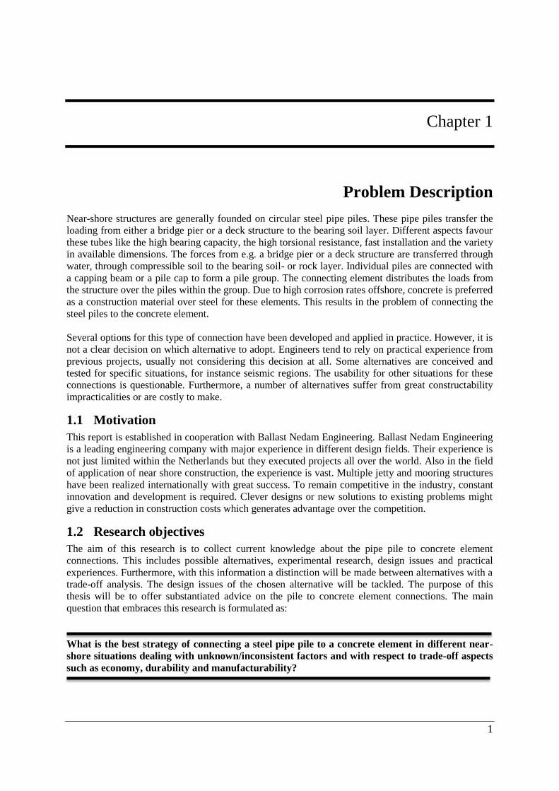
1. Problem Description
Near-shore structures are generally founded on circular steel pipe piles. These pipe piles transfer the
loading from either a bridge pier or a deck structure to the bearing soil layer. Different aspects favour
these tubes like the high bearing capacity, the high torsional resistance, fast installation and the variety
in available dimensions. The forces from e.g. a bridge pier or a deck structure are transferred through
water, through compressible soil to the bearing soil- or rock layer. Individual piles are connected with
a capping beam or a pile cap to form a pile group. The connecting element distributes the loads from
the structure over the piles within the group. Due to high corrosion rates offshore, concrete is preferred
as a construction material over steel for these elements. This results in the problem of connecting the
steel piles to the concrete element.
Several options for this type of connection have been developed and applied in practice. However, it is
not a clear decision on which alternative to adopt. Engineers tend to rely on practical experience from
previous projects, usually not considering this decision at all. Some alternatives are conceived and
tested for specific situations, for instance seismic regions. The usability for other situations for these
connections is questionable. Furthermore, a number of alternatives suffer from great constructability
impracticalities or are costly to make.
Motivation 1.1
This report is established in cooperation with Ballast Nedam Engineering. Ballast Nedam Engineering
is a leading engineering company with major experience in different design fields. Their experience is
not just limited within the Netherlands but they executed projects all over the world. Also in the field
of application of near shore construction, the experience is vast. Multiple jetty and mooring structures
have been realized internationally with great success. To remain competitive in the industry, constant
innovation and development is required. Clever designs or new solutions to existing problems might
give a reduction in construction costs which generates advantage over the competition.
Research objectives 1.2
The aim of this research is to collect current knowledge about the pipe pile to concrete element
connections. This includes possible alternatives, experimental research, design issues and practical
experiences. Furthermore, with this information a distinction will be made between alternatives with a
trade-off analysis. The design issues of the chosen alternative will be tackled. The purpose of this
thesis will be to offer substantiated advice on the pile to concrete element connections. The main
question that embraces this research is formulated as:
What is the best strategy of connecting a steel pipe pile to a concrete element in different near-
shore situations dealing with unknown/inconsistent factors and with respect to trade-off aspects
such as economy, durability and manufacturability?
Problem Description
2
To answer this question, a literature research will be carried out about possible joining options. With
the help of the expertise within Ballast Nedam Engineering, more information about practical
experience, like costs, manufacturability etc. will be obtained.
Outline 1.3
The outline of this document is as follows:
The general picture concerning the near-shore structure is given in Chapter 2. Aspects to take into
account in making a proper decision are identified. The developed alternatives are listed and
subdivided into the production method of the capping beam in Chapter 3. Chapter 4 deals with the
decision model in which a distinction is made between the remaining options from Chapter 3. Trade-
off aspects like the manufacturability, costs and construction times are considered.
The analysis results in one single alternative which is preferred on this basis. The behaviour of this
connection is deepened in Chapter 5. A distinction is made between two axial load transfer methods.
The first one, about the natural bond stress, is elaborated in more detail in Chapter 6. An analytical
bond model is proposed in Chapter 7 and verified to test data in Chapter 8. The second transfer
method is deepened in Chapter 9. The following chapter discusses a proposition for the bending
moment capacity. In the final chapter, the main conclusions are presented and recommendations for
future research are given.
3
Chapter 2
2. Applications & Background
The considered pipe pile to concrete element connections are applied in multiple applications with
varying properties. Structures in which the joints are adopted are briefly discussed together with more
background information regarding production methods of the pile and the concrete element, design
influences and the loading which can be expected. This will reveal a number of issues to keep in mind
for further design.
Applications 2.1
The function of the steel pipe piles is to transfer the loading from the superstructure to the more
compact and less compressible soil- or rock layer (Tomlinson et al. (2008)). In offshore situations, this
is through water, through compressible soil to the bearing sand- or rock layer. The structure is
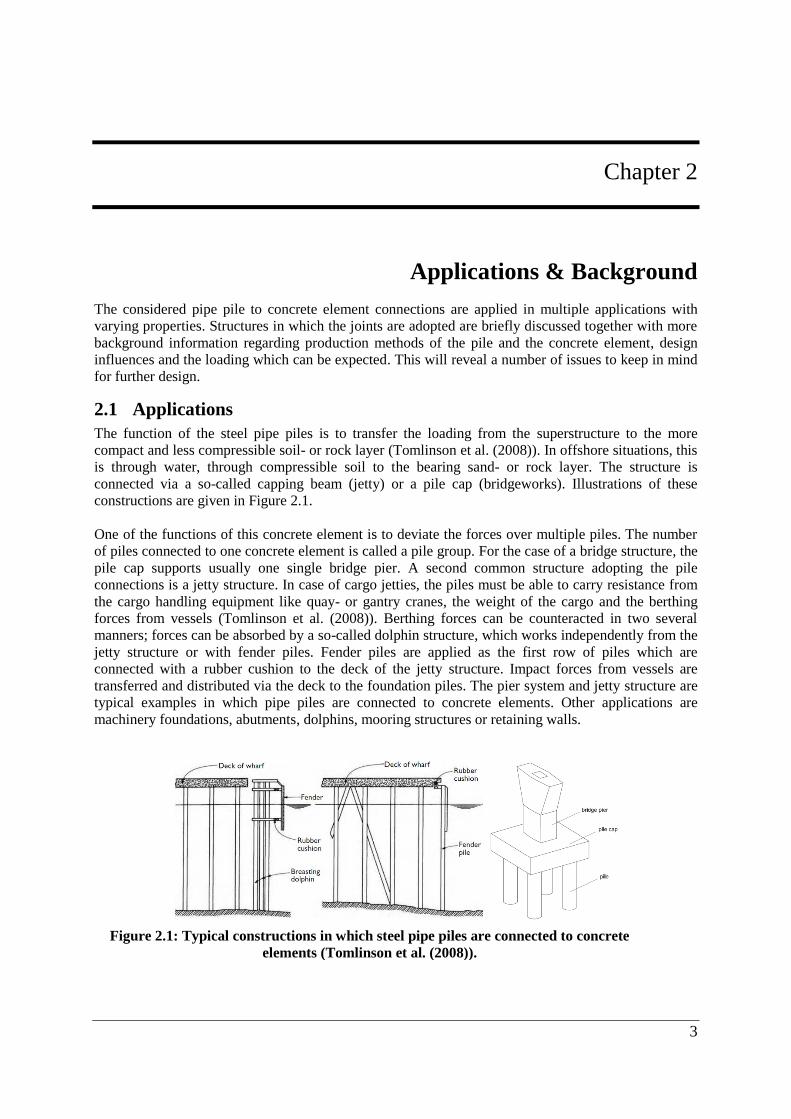
connected via a so-called capping beam (jetty) or a pile cap (bridgeworks). Illustrations of these
constructions are given in Figure 2.1.
One of the functions of this concrete element is to deviate the forces over multiple piles. The number
of piles connected to one concrete element is called a pile group. For the case of a bridge structure, the
pile cap supports usually one single bridge pier. A second common structure adopting the pile
connections is a jetty structure. In case of cargo jetties, the piles must be able to carry resistance from
the cargo handling equipment like quay- or gantry cranes, the weight of the cargo and the berthing
forces from vessels (Tomlinson et al. (2008)). Berthing forces can be counteracted in two several
manners; forces can be absorbed by a so-called dolphin structure, which works independently from the
jetty structure or with fender piles. Fender piles are applied as the first row of piles which are
connected with a rubber cushion to the deck of the jetty structure. Impact forces from vessels are
transferred and distributed via the deck to the foundation piles. The pier system and jetty structure are
typical examples in which pipe piles are connected to concrete elements. Other applications are
machinery foundations, abutments, dolphins, mooring structures or retaining walls.
Figure 2.1: Typical constructions in which steel pipe piles are connected to concrete
elements (Tomlinson et al. (2008)).
Applications & Background
4
2.1.1 Force deviation
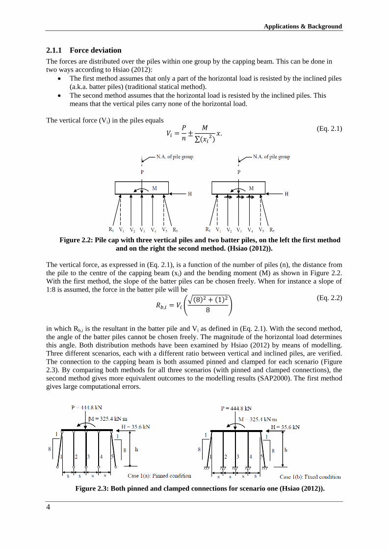
The forces are distributed over the piles within one group by the capping beam. This can be done in
two ways according to Hsiao (2012):
The first method assumes that only a part of the horizontal load is resisted by the inclined piles
(a.k.a. batter piles) (traditional statical method).
The second method assumes that the horizontal load is resisted by the inclined piles. This
means that the vertical piles carry none of the horizontal load.
The vertical force (Vi) in the piles equals
𝑉𝑖 =
𝑃
𝑛±
𝑀
∑(𝑥𝑖2)𝑥.
(Eq. 2.1)
Figure 2.2: Pile cap with three vertical piles and two batter piles, on the left the first method
and on the right the second method. (Hsiao (2012)).
The vertical force, as expressed in (Eq. 2.1), is a function of the number of piles (n), the distance from
the pile to the centre of the capping beam (xi) and the bending moment (M) as shown in Figure 2.2.
With the first method, the slope of the batter piles can be chosen freely. When for instance a slope of
1:8 is assumed, the force in the batter pile will be
𝑅𝑏,𝑖 = 𝑉𝑖 (
√(8)2 + (1)2
8)
(Eq. 2.2)
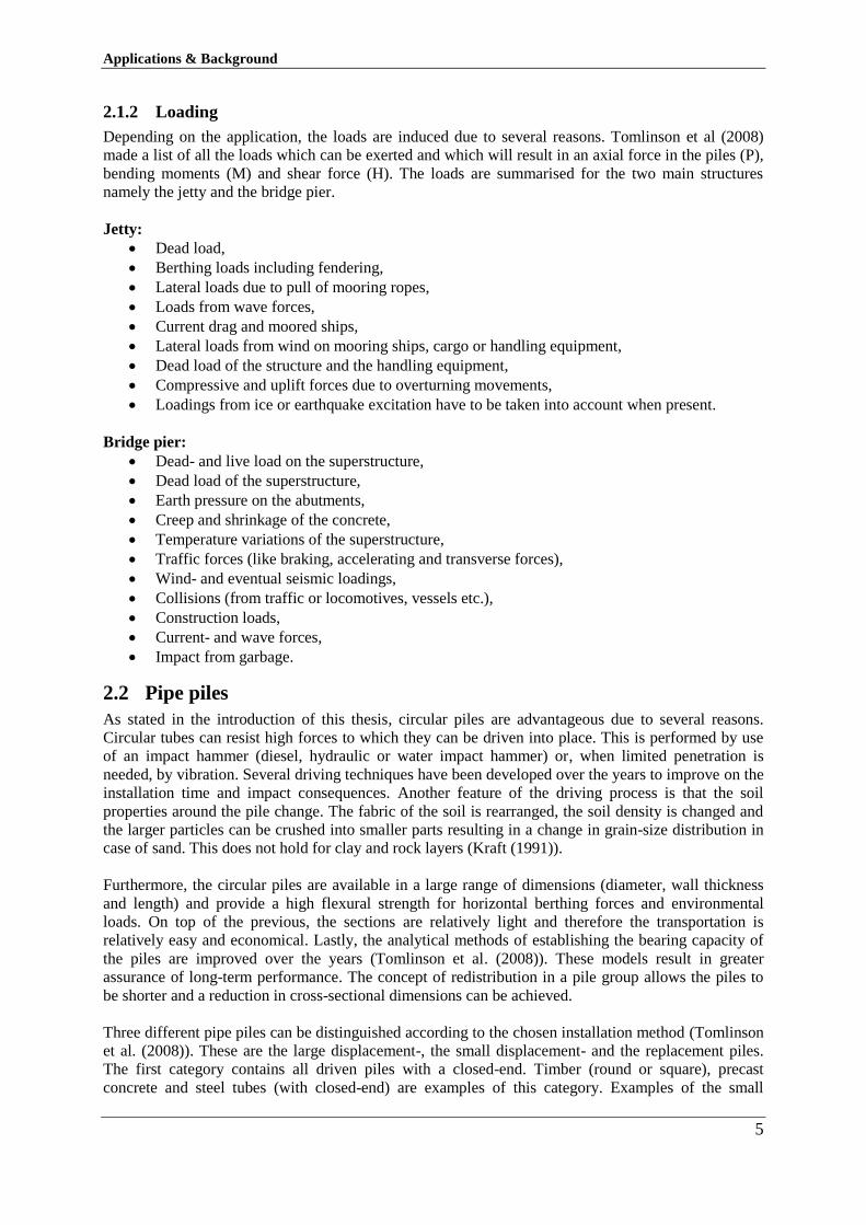
in which Rb,i is the resultant in the batter pile and Vi as defined in (Eq. 2.1). With the second method,
the angle of the batter piles cannot be chosen freely. The magnitude of the horizontal load determines
this angle. Both distribution methods have been examined by Hsiao (2012) by means of modelling.
Three different scenarios, each with a different ratio between vertical and inclined piles, are verified.
The connection to the capping beam is both assumed pinned and clamped for each scenario (Figure
2.3). By comparing both methods for all three scenarios (with pinned and clamped connections), the
second method gives more equivalent outcomes to the modelling results (SAP2000). The first method
gives large computational errors.
Figure 2.3: Both pinned and clamped connections for scenario one (Hsiao (2012)).
Applications & Background
5
2.1.2 Loading
Depending on the application, the loads are induced due to several reasons. Tomlinson et al (2008)
made a list of all the loads which can be exerted and which will result in an axial force in the piles (P),
bending moments (M) and shear force (H). The loads are summarised for the two main structures
namely the jetty and the bridge pier.
Jetty:
Dead load,
Berthing loads including fendering,
Lateral loads due to pull of mooring ropes,
Loads from wave forces,
Current drag and moored ships,
Lateral loads from wind on mooring ships, cargo or handling equipment,
Dead load of the structure and the handling equipment,
Compressive and uplift forces due to overturning movements,
Loadings from ice or earthquake excitation have to be taken into account when present.
Bridge pier:
Dead- and live load on the superstructure,
Dead load of the superstructure,
Earth pressure on the abutments,
Creep and shrinkage of the concrete,
Temperature variations of the superstructure,
Traffic forces (like braking, accelerating and transverse forces),
Wind- and eventual seismic loadings,
Collisions (from traffic or locomotives, vessels etc.),
Construction loads,
Current- and wave forces,
Impact from garbage.
Pipe piles 2.2
As stated in the introduction of this thesis, circular piles are advantageous due to several reasons.
Circular tubes can resist high forces to which they can be driven into place. This is performed by use
of an impact hammer (diesel, hydraulic or water impact hammer) or, when limited penetration is
needed, by vibration. Several driving techniques have been developed over the years to improve on the
installation time and impact consequences. Another feature of the driving process is that the soil
properties around the pile change. The fabric of the soil is rearranged, the soil density is changed and
the larger particles can be crushed into smaller parts resulting in a change in grain-size distribution in
case of sand. This does not hold for clay and rock layers (Kraft (1991)).
Furthermore, the circular piles are available in a large range of dimensions (diameter, wall thickness
and length) and provide a high flexural strength for horizontal berthing forces and environmental
loads. On top of the previous, the sections are relatively light and therefore the transportation is
relatively easy and economical. Lastly, the analytical methods of establishing the bearing capacity of
the piles are improved over the years (Tomlinson et al. (2008)). These models result in greater
assurance of long-term performance. The concept of redistribution in a pile group allows the piles to
be shorter and a reduction in cross-sectional dimensions can be achieved.
Three different pipe piles can be distinguished according to the chosen installation method (Tomlinson
et al. (2008)). These are the large displacement-, the small displacement- and the replacement piles.
The first category contains all driven piles with a closed-end. Timber (round or square), precast
concrete and steel tubes (with closed-end) are examples of this category. Examples of the small
Applications & Background
6
displacement piles are open-ended steel pipes or open-ended prestressed or precast concrete piles. The
pile is called open-ended when the soil is able to enter the pile (no further provisions are given).
Nonetheless, this research is limited to steel piles only.
Pipe piles transfer the forcing to the bearing soil layer via either the tip of the pile (point bearing piles),
friction (friction piles), and lateral force transfer or tension forces via shaft friction. Due to overturning
moments (due to wind or berthing loads), piles can be loaded in tension which can be permanent or
temporally. The resistance of such a tension pile contains the own weight of the pile, the friction
between the pile shaft and the surrounding soil and the adhesion between pile and soil (FinnRa
(2000)).
2.2.1 Production methods
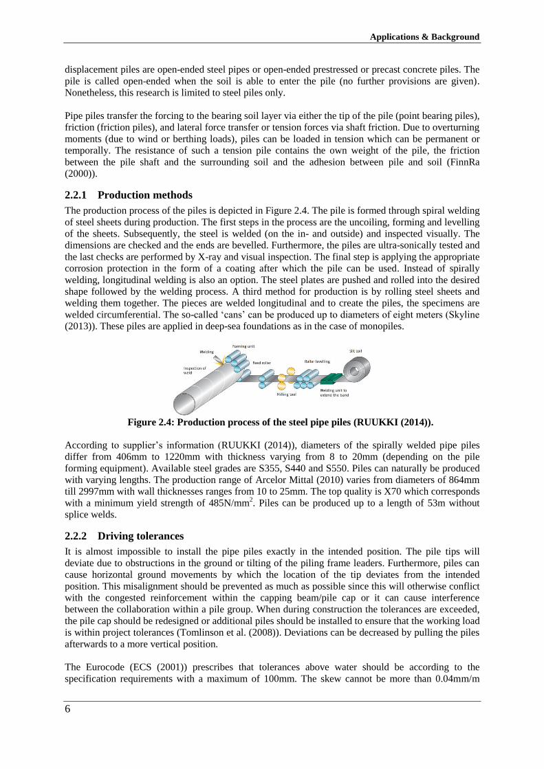
The production process of the piles is depicted in Figure 2.4. The pile is formed through spiral welding
of steel sheets during production. The first steps in the process are the uncoiling, forming and levelling
of the sheets. Subsequently, the steel is welded (on the in- and outside) and inspected visually. The
dimensions are checked and the ends are bevelled. Furthermore, the piles are ultra-sonically tested and
the last checks are performed by X-ray and visual inspection. The final step is applying the appropriate
corrosion protection in the form of a coating after which the pile can be used. Instead of spirally
welding, longitudinal welding is also an option. The steel plates are pushed and rolled into the desired
shape followed by the welding process. A third method for production is by rolling steel sheets and
welding them together. The pieces are welded longitudinal and to create the piles, the specimens are
welded circumferential. The so-called ‘cans’ can be produced up to diameters of eight meters (Skyline
(2013)). These piles are applied in deep-sea foundations as in the case of monopiles.
Figure 2.4: Production process of the steel pipe piles (RUUKKI (2014)).
According to supplier’s information (RUUKKI (2014)), diameters of the spirally welded pipe piles
differ from 406mm to 1220mm with thickness varying from 8 to 20mm (depending on the pile
forming equipment). Available steel grades are S355, S440 and S550. Piles can naturally be produced
with varying lengths. The production range of Arcelor Mittal (2010) varies from diameters of 864mm
till 2997mm with wall thicknesses ranges from 10 to 25mm. The top quality is X70 which corresponds
with a minimum yield strength of 485N/mm2. Piles can be produced up to a length of 53m without
splice welds.
2.2.2 Driving tolerances
It is almost impossible to install the pipe piles exactly in the intended position. The pile tips will
deviate due to obstructions in the ground or tilting of the piling frame leaders. Furthermore, piles can
cause horizontal ground movements by which the location of the tip deviates from the intended
position. This misalignment should be prevented as much as possible since this will otherwise conflict
with the congested reinforcement within the capping beam/pile cap or it can cause interference
between the collaboration within a pile group. When during construction the tolerances are exceeded,
the pile cap should be redesigned or additional piles should be installed to ensure that the working load
is within project tolerances (Tomlinson et al. (2008)). Deviations can be decreased by pulling the piles
afterwards to a more vertical position.
The Eurocode (ECS (2001)) prescribes that tolerances above water should be according to the
specification requirements with a maximum of 100mm. The skew cannot be more than 0.04mm/m
Applications & Background
7
pile. These values need to be adopted for both vertical- and batter piles installed as displacement piles.
According to ECS (2011e), the maximum deviation is 100mm for pipe piles with a diameter (Dp)
smaller then 1.0m, 0.1Dp for 1.0m≤Dp≤1.5m and 150mm for Dp>1.5m in case of bored piles.
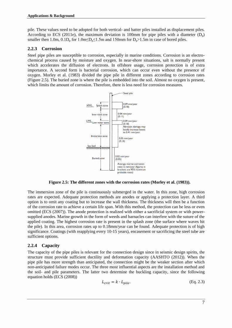
2.2.3 Corrosion
Steel pipe piles are susceptible to corrosion, especially in marine conditions. Corrosion is an electro-
chemical process caused by moisture and oxygen. In near-shore situations, salt is normally present
which accelerates the diffusion of electrons. In offshore usage, corrosion protection is of extra
importance. A second form is bacterial corrosion, which can occur even without the presence of
oxygen. Morley et al. (1983) divided the pipe pile in different zones according to corrosion rates
(Figure 2.5). The buried zone is where the pile is embedded into the soil. Almost no oxygen is present,
which limits the amount of corrosion. Therefore, there is less need for corrosion measures.
Figure 2.5: The different zones with the corrosion rates (Morley et al. (1983)).
The immersion zone of the pile is continuously submerged in the water. In this zone, high corrosion
rates are expected. Adequate protection methods are anodes or applying a protection layer. A third
option is to omit any coating but to increase the wall thickness. The thickness will then be a function
of the corrosion rate to achieve a certain life span. With this method, the protection can be less or even
omitted (ECS (2007)). The anode protection is realized with either a sacrificial system or with power-
supplied anodes. Marine growth in the form of weeds and barnacles can interfere with the suture of the
applied coating. The highest corrosion rate is present in the splash zone (the surface where waves hit
the pile). In this area, corrosion rates up to 0.18mm/year can be found. Adequate protection is of high
significance. Coatings (with reapplying every 10-15 years), encasement or sacrificing the steel tube are
sufficient options.
2.2.4 Capacity
The capacity of the pipe piles is relevant for the connection design since in seismic design spirits, the
structure must provide sufficient ductility and deformation capacity (AASHTO (2012)). When the
pipe pile has more strength than anticipated, the connection might be the weaker section after which
non-anticipated failure modes occur. The three most influential aspects are the installation method and
the soil- and pile parameters. The latter two determine the buckling capacity, since the following
equation holds (ECS (2008))
𝐿𝑐𝑟𝑖𝑡 = 𝑘 ∙ 𝐿𝑝𝑖𝑙𝑒 . (Eq. 2.3)
Applications & Background
8
The buckling length (Lpile) is a function of the length above the firm soil and the stiffness of the
connection (k). In the case of soft soil, the firm layer is far down after which a long buckling length is
found. The connection design can counteract this effect.
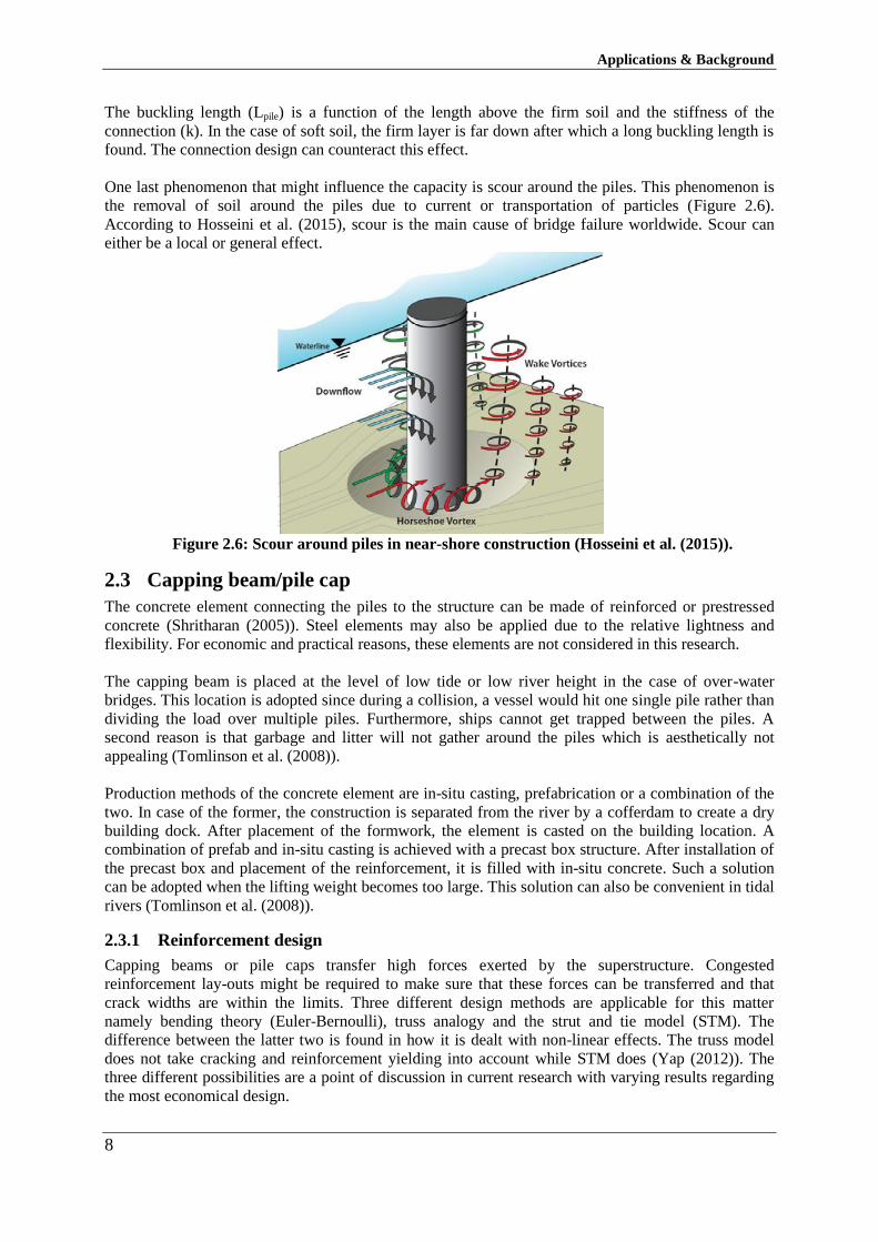
One last phenomenon that might influence the capacity is scour around the piles. This phenomenon is
the removal of soil around the piles due to current or transportation of particles (Figure 2.6).
According to Hosseini et al. (2015), scour is the main cause of bridge failure worldwide. Scour can
either be a local or general effect.
Figure 2.6: Scour around piles in near-shore construction (Hosseini et al. (2015)).
Capping beam/pile cap 2.3
The concrete element connecting the piles to the structure can be made of reinforced or prestressed
concrete (Shritharan (2005)). Steel elements may also be applied due to the relative lightness and
flexibility. For economic and practical reasons, these elements are not considered in this research.
The capping beam is placed at the level of low tide or low river height in the case of over-water
bridges. This location is adopted since during a collision, a vessel would hit one single pile rather than
dividing the load over multiple piles. Furthermore, ships cannot get trapped between the piles. A
second reason is that garbage and litter will not gather around the piles which is aesthetically not
appealing (Tomlinson et al. (2008)).
Production methods of the concrete element are in-situ casting, prefabrication or a combination of the
two. In case of the former, the construction is separated from the river by a cofferdam to create a dry
building dock. After placement of the formwork, the element is casted on the building location. A
combination of prefab and in-situ casting is achieved with a precast box structure. After installation of
the precast box and placement of the reinforcement, it is filled with in-situ concrete. Such a solution
can be adopted when the lifting weight becomes too large. This solution can also be convenient in tidal
rivers (Tomlinson et al. (2008)).
2.3.1 Reinforcement design
Capping beams or pile caps transfer high forces exerted by the superstructure. Congested
reinforcement lay-outs might be required to make sure that these forces can be transferred and that
crack widths are within the limits. Three different design methods are applicable for this matter
namely bending theory (Euler-Bernoulli), truss analogy and the strut and tie model (STM). The
difference between the latter two is found in how it is dealt with non-linear effects. The truss model
does not take cracking and reinforcement yielding into account while STM does (Yap (2012)). The
three different possibilities are a point of discussion in current research with varying results regarding
the most economical design.
Applications & Background
9
Raj et al. (2008) conducted an experiment on all three different theories and concluded that the STM
leads to the lowest cost regarding reinforcement. Contrary to the conclusion from Raj et al. (2008), is
the result from Nori et al. (2007). They state that an STM will result in more flexural reinforcement
than the beam theory (bending theory). The reason for this difference is that no shear reinforcement is
needed. This conclusion is based on strut and tie models for pile caps with different numbers of piles
and with different loading situations. Furthermore, they conclude that an STM cannot be used for
loading situations which include bending moments.
According to Souza et al. (2009), this inconsistency in test results between Raj et al. (2008) and Nori
et al. (2007) can be explained by two factors. The first is the position of the critical section for bending
and the second is the position of the nodal zone underneath the column. Therefore it is difficult to state
that the STM is more efficient in general. Added to this conclusion is that the strut and tie model
represents the flow of forces better than the sectional design methods.
Conclusion 2.4
The backgrounds concerning the steel piles, the concrete element and the possible applications are
investigated in this chapter. Important issues are pile tip deviations up to 150mm, steel corrosion,
capacity of the piles and the reinforcement design of the concrete element. These matters should
definitely be taken into account.
The connection type investigated in this report, finds its application in for instance jetty structures,
bridgeworks and mooring structures. Due to the several possible applications, multiple designs have
been made over the years. These are examined in the following chapter.

Applications & Background
10
11
Chapter 3
3. Alternatives
Resulting from the multiple applications to which the considered connections are applicable,
numerous alternatives have been developed over the years. These variants are subjected to a great deal
of research about failure mechanisms, strength properties and seismic behaviour. An overview of the
current knowledge is reported and alternatives are listed.
Design strategies 3.1
During this literature research, two design strategies are acknowledged. Most of the found research
concerns the usability in areas with seismic activity. The intention for those areas is completely
different since it focusses on different principles.
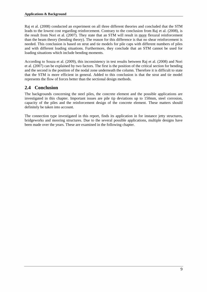
3.1.1 Seismic design strategy
Seismic design is aimed at ductility within the connection/system. According to the AASHTO (2012),
the piles are the members that are able to provide this capacity the most. Their reasoning is that the
piles provide a high energy-dissipation and rotation capacity. Prior to failure of the connection, the
piles should have formed plastic hinges. As seen in the left of Figure 3.1, the pile tends to buckle to
which plastic hinges are formed. The pile will tear at the location of the local buckle when the load is
further increased as displayed in the right of Figure 3.1.
Experimental research for seismic purposes is aimed at demonstration of the proper failure
mechanism. These seismic systems are called capacity-protected, since the connection provides higher
cyclic loading strength in comparison to the adjacent members (NCHRP (2011)).
Figure 3.1: Local buckling of the pipe piles on the left and tearing of the tube at the position
of the local buckle at the right (Stephens et al. (2014)).
Due to the unpredictable character of seismic activity, design forces are taken twice the expected
magnitude. An overstrength factor is introduced to make sure that the correct failure mechanism
occurs. This factor increases the column capacity by 1.25 in order to make sure that all other parts in
the system are stronger than the column. It happens that columns are stronger than accounted for due
to miscommunications or delivery reasons (AASHTO (2012)).
Alternatives
12
3.1.2 Non-seismic design strategy
Non-seismic design aims at adequate strength during service and exceptional conditions. Components
should be designed according to the appropriate design code to provide adequate levels of safety.
Choosing between alternatives is based on practical and economic reasons in contrast to the previous
paragraph. These alternatives are likely to be too expensive in non-seismic application.
Connection alternatives 3.2
To be able to make a distinction between the options, the construction method of the capping beam is
used. Following from the previous chapter, it is seen that this element can be produced either in-situ or
prefab. The results from experimental research are added for every connection design.
3.2.1 In-situ capping beam/pile cap
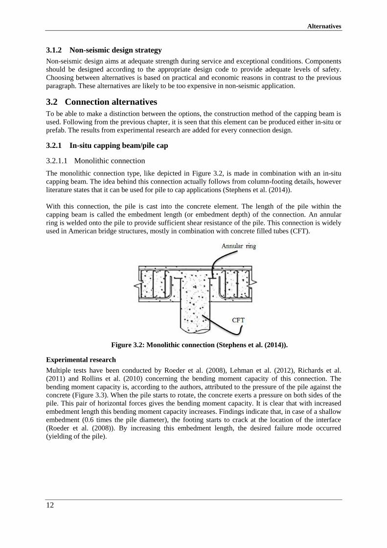
3.2.1.1 Monolithic connection
The monolithic connection type, like depicted in Figure 3.2, is made in combination with an in-situ
capping beam. The idea behind this connection actually follows from column-footing details, however
literature states that it can be used for pile to cap applications (Stephens et al. (2014)).
With this connection, the pile is cast into the concrete element. The length of the pile within the
capping beam is called the embedment length (or embedment depth) of the connection. An annular
ring is welded onto the pile to provide sufficient shear resistance of the pile. This connection is widely
used in American bridge structures, mostly in combination with concrete filled tubes (CFT).
Figure 3.2: Monolithic connection (Stephens et al. (2014)).
Experimental research
Multiple tests have been conducted by Roeder et al. (2008), Lehman et al. (2012), Richards et al.
(2011) and Rollins et al. (2010) concerning the bending moment capacity of this connection. The
bending moment capacity is, according to the authors, attributed to the pressure of the pile against the
concrete (Figure 3.3). When the pile starts to rotate, the concrete exerts a pressure on both sides of the
pile. This pair of horizontal forces gives the bending moment capacity. It is clear that with increased
embedment length this bending moment capacity increases. Findings indicate that, in case of a shallow
embedment (0.6 times the pile diameter), the footing starts to crack at the location of the interface
(Roeder et al. (2008)). By increasing this embedment length, the desired failure mode occurred
(yielding of the pile).
Alternatives
13
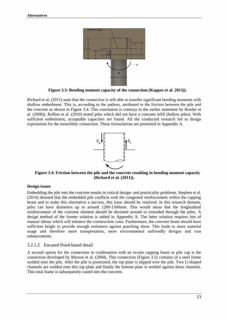
Figure 3.3: Bending moment capacity of the connection (Kappes et al. 2013)).
Richard et al. (2011) state that the connection is still able to transfer significant bending moments with
shallow embedment. This is, according to the authors, attributed to the friction between the pile and
the concrete as shown in Figure 3.4. This conclusion is contrary to the earlier statement by Roeder et
al. (2008)). Rollins et al. (2010) tested piles which did not have a concrete infill (hollow piles). With
sufficient embedment, acceptable capacities are found. All the conducted research led to design
expressions for the monolithic connection. These formulations are presented in Appendix A.
Figure 3.4: Friction between the pile and the concrete resulting in bending moment capacity
(Richard et al. (2011)).
Design issues
Embedding the pile into the concrete results in critical design- and practicality problems. Stephen et al.
(2014) denoted that the embedded pile conflicts with the congested reinforcement within the capping
beam and to make this alternative a success, this issue should be resolved. In this research domain,
piles can have diameters up to around 1200-1500mm. This would mean that the longitudinal
reinforcement of the concrete element should be deviated around or extended through the piles. A
design method of the former solution is added in Appendix A. The latter solution requires lots of
manual labour which will enhance the construction costs. Furthermore, the concrete beam should have
sufficient height to provide enough resistance against punching shear. This leads to more material
usage and therefore more transportation, more environmental unfriendly designs and cost
enhancements.
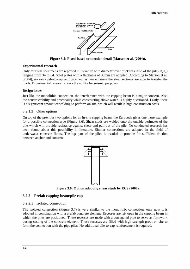
3.2.1.2 Encased fixed-based detail
A second option for the connection in combination with an in-situ capping beam or pile cap is the
connection developed by Marson et al. (2004). This connection (Figure 3.5) contains of a steel frame
welded onto the pile. After the pile is positioned, the top plate is slipped over the pile. Two U-shaped
channels are welded onto this top plate and finally the bottom plate is welded against these channels.
This total frame is subsequently casted into the concrete.
Alternatives
14
Figure 3.5: Fixed-based connection detail (Marson et al. (2004)).
Experimental research
Only four test specimens are reported in literature with diameter over thickness ratio of the pile (Dp/tp)
ranging from 34 to 64. Steel plates with a thickness of 30mm are adopted. According to Marson et al.
(2004), no extra pile-to-cap reinforcement is needed since the steel sections are able to transfer the
loads. Experimental research shows the ability for seismic purposes.
Design issues
Just like the monolithic connection, the interference with the capping beam is a major concern. Also
the constructability and practicality while constructing above water, is highly questioned. Lastly, there
is a significant amount of welding to perform on site, which will result in high construction costs.
3.2.1.3 Other options
On top of the previous two options for an in-situ capping beam, the Eurocode gives one more example
for a possible connection type (Figure 3.6). Shear studs are welded onto the outside perimeter of the
pile which will provide resistance against shear and pull-out of the pile. No conducted research has
been found about this possibility in literature. Similar connections are adopted in the field of
underwater concrete floors. The top part of the piles is treaded to provide for sufficient friction
between anchor and concrete.
Figure 3.6: Option adopting shear studs by ECS (2008).
3.2.2 Prefab capping beam/pile cap
3.2.2.1 Isolated connection
The isolated connection (Figure 3.7) is very similar to the monolithic connection, only now it is
adopted in combination with a prefab concrete element. Recesses are left open in the capping beam in
which the piles are positioned. These recesses are made with a corrugated pipe to serve as formwork
during casting of the concrete element. These recesses are filled with high strength grout on site to
form the connection with the pipe piles. No additional pile-to-cap reinforcement is required.
Alternatives
15
Figure 3.7: Isolated connection (Stephens et al. (2014)).
Experimental research
Research about the isolated connection is associated with research of the monolithic from section
3.2.1.1. The results as presented in Appendix A are also applicable to this connection type.
Design issues
The same design issues apply to the isolated connection as to the monolithic variant due to the
similarities. Adopting this connection in a pile-to-cap construction, the recesses should provide for the
ability of pile deviations. A problem arises when these deviations are larger than the recesses can
provide. Secondly, the grout is poured immediately after the element is positioned, which gives cause
to new issues. The space around the pile should be closed and sealed, to which the grout is poured
from either below or above the capping beam. This results in impracticalities at the workplace.
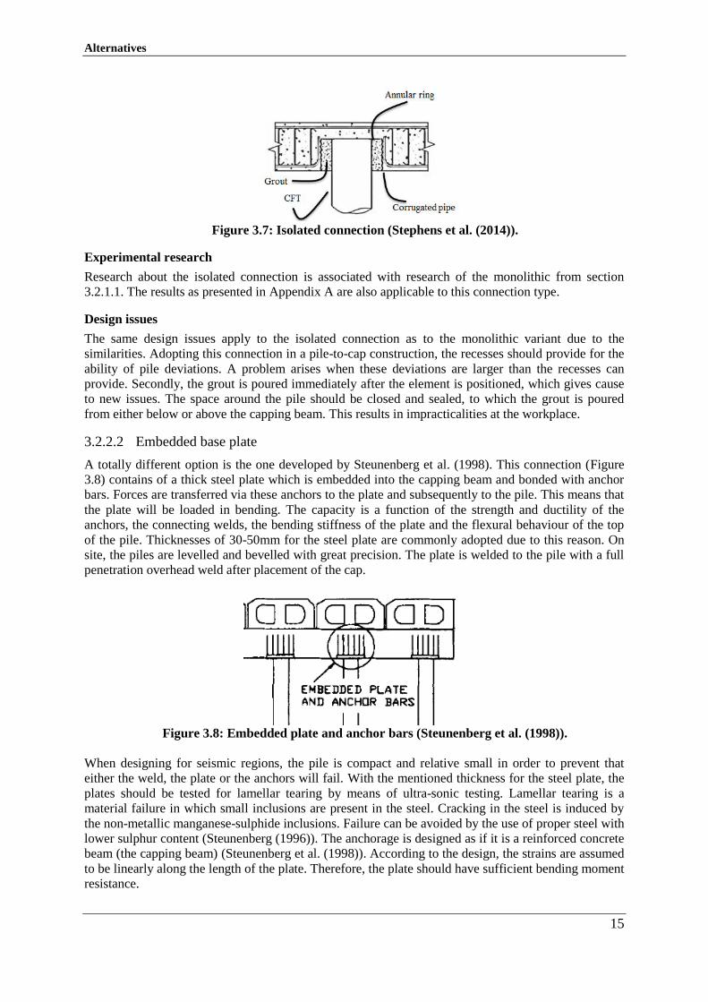
3.2.2.2 Embedded base plate
A totally different option is the one developed by Steunenberg et al. (1998). This connection (Figure
3.8) contains of a thick steel plate which is embedded into the capping beam and bonded with anchor
bars. Forces are transferred via these anchors to the plate and subsequently to the pile. This means that
the plate will be loaded in bending. The capacity is a function of the strength and ductility of the
anchors, the connecting welds, the bending stiffness of the plate and the flexural behaviour of the top
of the pile. Thicknesses of 30-50mm for the steel plate are commonly adopted due to this reason. On
site, the piles are levelled and bevelled with great precision. The plate is welded to the pile with a full
penetration overhead weld after placement of the cap.
Figure 3.8: Embedded plate and anchor bars (Steunenberg et al. (1998)).
When designing for seismic regions, the pile is compact and relative small in order to prevent that
either the weld, the plate or the anchors will fail. With the mentioned thickness for the steel plate, the
plates should be tested for lamellar tearing by means of ultra-sonic testing. Lamellar tearing is a
material failure in which small inclusions are present in the steel. Cracking in the steel is induced by
the non-metallic manganese-sulphide inclusions. Failure can be avoided by the use of proper steel with
lower sulphur content (Steunenberg (1996)). The anchorage is designed as if it is a reinforced concrete
beam (the capping beam) (Steunenberg et al. (1998)). According to the design, the strains are assumed
to be linearly along the length of the plate. Therefore, the plate should have sufficient bending moment
resistance.
Alternatives
16
The welding of the steel plate to the circular pile has to be performed by a qualified welder with the
appropriate inspection afterwards. When weld faults are found, it needs to be repaired and rechecked.
Experimental research
Research has been performed by Steunenberg et al. (1998). Only one test specimen is examined with a
diameter of 324mm and a wall thickness of 12.7mm. The yield strength of the pile appeared to be
almost 30% higher than expected which indicates the usefulness of the overstrength factor (like
explained in section 3.1.1). Despite the exceedance of this factor, the connection still fulfilled the
requirements and the appropriate failure mechanism was found.
Design issues
The large thickness of the plate is cause for ultra-sonic testing and high workshop specifications. The
required tools to handle such a plate are expensive and not present in every region. Holes are drilled in
the plate in which the anchor bars are positioned. This means double welding of the anchor bars on
both sides of the plate, which is costly to perform. Furthermore, deviations in pile tip position need to
be accounted for in the anchor plan resulting in a lot of anchors and large plate dimensions. The plates
are welded to the piles with overhead welds on site. Only special trained and licensed workmen may
perform this weld. Nonetheless the quality of the welders, weld defects are hard to prevent.
3.2.3 Both prefab and in-situ
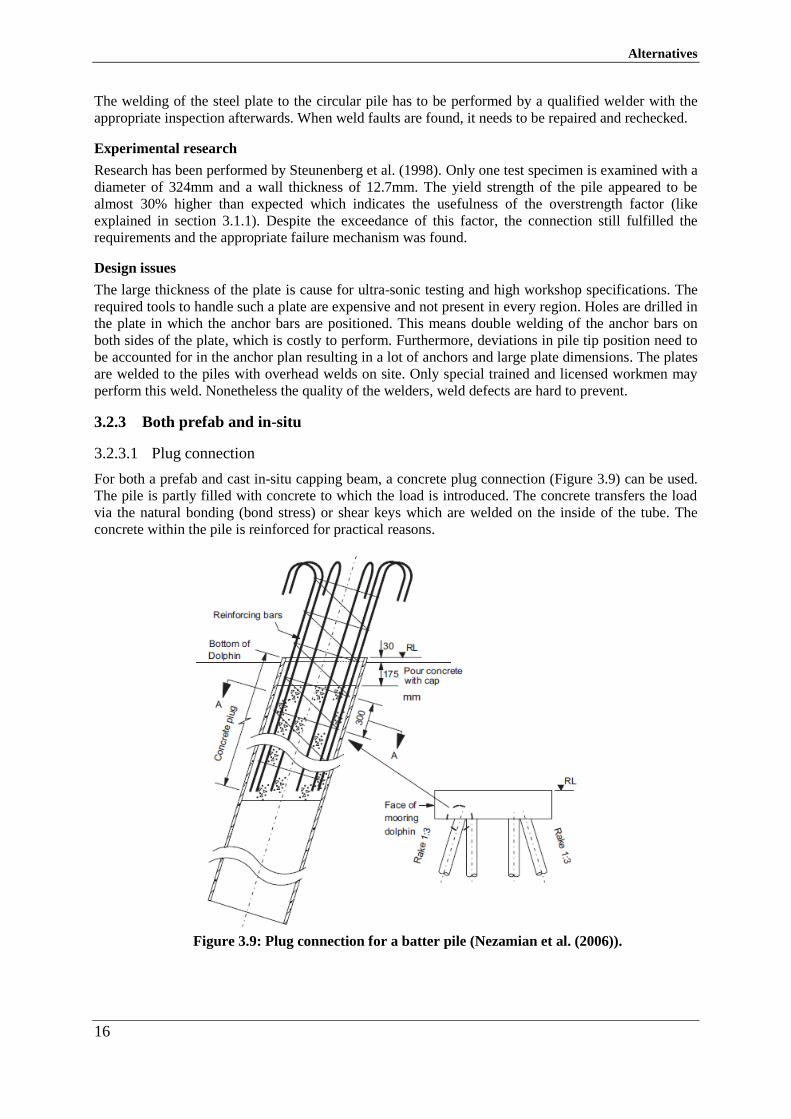
3.2.3.1 Plug connection
For both a prefab and cast in-situ capping beam, a concrete plug connection (Figure 3.9) can be used.
The pile is partly filled with concrete to which the load is introduced. The concrete transfers the load
via the natural bonding (bond stress) or shear keys which are welded on the inside of the tube. The
concrete within the pile is reinforced for practical reasons.
Figure 3.9: Plug connection for a batter pile (Nezamian et al. (2006)).
Alternatives
17
Experimental research
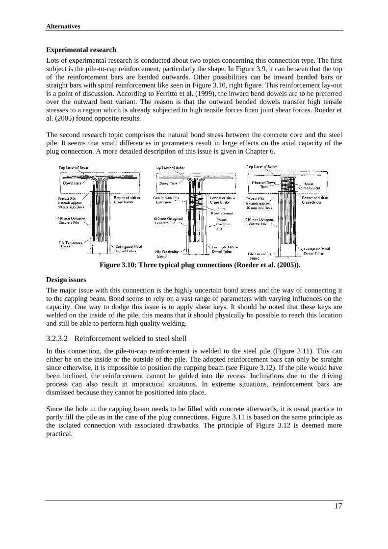
Lots of experimental research is conducted about two topics concerning this connection type. The first
subject is the pile-to-cap reinforcement, particularly the shape. In Figure 3.9, it can be seen that the top
of the reinforcement bars are bended outwards. Other possibilities can be inward bended bars or
straight bars with spiral reinforcement like seen in Figure 3.10, right figure. This reinforcement lay-out
is a point of discussion. According to Ferritto et al. (1999), the inward bend dowels are to be preferred
over the outward bent variant. The reason is that the outward bended dowels transfer high tensile
stresses to a region which is already subjected to high tensile forces from joint shear forces. Roeder et
al. (2005) found opposite results.
The second research topic comprises the natural bond stress between the concrete core and the steel
pile. It seems that small differences in parameters result in large effects on the axial capacity of the
plug connection. A more detailed description of this issue is given in Chapter 6.
Figure 3.10: Three typical plug connections (Roeder et al. (2005)).
Design issues
The major issue with this connection is the highly uncertain bond stress and the way of connecting it
to the capping beam. Bond seems to rely on a vast range of parameters with varying influences on the
capacity. One way to dodge this issue is to apply shear keys. It should be noted that these keys are
welded on the inside of the pile, this means that it should physically be possible to reach this location
and still be able to perform high quality welding.
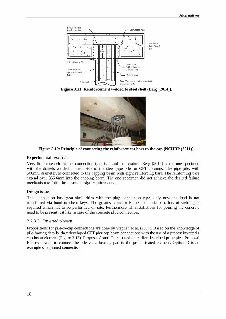
3.2.3.2 Reinforcement welded to steel shell
In this connection, the pile-to-cap reinforcement is welded to the steel pile (Figure 3.11). This can
either be on the inside or the outside of the pile. The adopted reinforcement bars can only be straight
since otherwise, it is impossible to position the capping beam (see Figure 3.12). If the pile would have
been inclined, the reinforcement cannot be guided into the recess. Inclinations due to the driving
process can also result in impractical situations. In extreme situations, reinforcement bars are
dismissed because they cannot be positioned into place.
Since the hole in the capping beam needs to be filled with concrete afterwards, it is usual practice to
partly fill the pile as in the case of the plug connections. Figure 3.11 is based on the same principle as
the isolated connection with associated drawbacks. The principle of Figure 3.12 is deemed more
practical.
Alternatives
18
Figure 3.11: Reinforcement welded to steel shell (Berg (2014)).
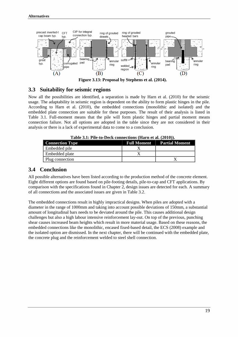
Figure 3.12: Principle of connecting the reinforcement bars to the cap (NCHRP (2011)).
Experimental research
Very little research on this connection type is found in literature. Berg (2014) tested one specimen
with the dowels welded to the inside of the steel pipe pile for CFT columns. The pipe pile, with
508mm diameter, is connected to the capping beam with eight reinforcing bars. The reinforcing bars
extend over 355.6mm into the capping beam. The one specimen did not achieve the desired failure
mechanism to fulfil the seismic design requirements.
Design issues
This connection has great similarities with the plug connection type, only now the load is not
transferred via bond or shear keys. The greatest concern is the economic part, lots of welding is
required which has to be performed on site. Furthermore, all installations for pouring the concrete
need to be present just like in case of the concrete plug connection.
3.2.3.3 Inverted t-beam
Propositions for pile-to-cap connections are done by Stephen et al. (2014). Based on the knowledge of
pile-footing details, they developed CFT pier cap beam connections with the use of a precast inverted-t
cap beam element (Figure 3.13). Proposal A and C are based on earlier described principles. Proposal
B uses dowels to connect the pile via a bearing pad to the prefabricated element. Option D is an
example of a pinned connection.
Alternatives
19
Figure 3.13: Proposal by Stephens et al. (2014).
Suitability for seismic regions 3.3
Now all the possibilities are identified, a separation is made by Harn et al. (2010) for the seismic
usage. The adaptability in seismic region is dependent on the ability to form plastic hinges in the pile.
According to Harn et al. (2010), the embedded connections (monolithic and isolated) and the
embedded plate connection are suitable for these purposes. The result of their analysis is listed in
Table 3.1. Full-moment means that the pile will form plastic hinges and partial moment means
connection failure. Not all options are adopted in the table since they are not considered in their
analysis or there is a lack of experimental data to come to a conclusion.
Table 3.1: Pile-to-Deck connections (Harn et al. (2010)).
Connection Type Full Moment Partial Moment
Embedded pile X
Embedded plate X
Plug connection X
Conclusion 3.4
All possible alternatives have been listed according to the production method of the concrete element.
Eight different options are found based on pile-footing details, pile-to-cap and CFT applications. By
comparison with the specifications found in Chapter 2, design issues are detected for each. A summary
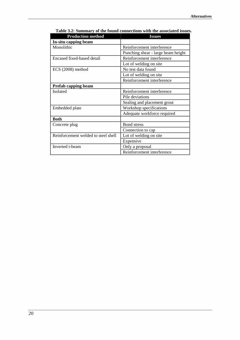
of all connections and the associated issues are given in Table 3.2.
The embedded connections result in highly impractical designs. When piles are adopted with a
diameter in the range of 1000mm and taking into account possible deviations of 150mm, a substantial
amount of longitudinal bars needs to be deviated around the pile. This causes additional design
challenges but also a high labour intensive reinforcement lay-out. On top of the previous, punching
shear causes increased beam heights which result in more material usage. Based on these reasons, the
embedded connections like the monolithic, encased fixed-based detail, the ECS (2008) example and
the isolated option are dismissed. In the next chapter, there will be continued with the embedded plate,
the concrete plug and the reinforcement welded to steel shell connection.
Alternatives
20
Table 3.2: Summary of the found connections with the associated issues.
Production method Issues
In-situ capping beam
Monolithic Reinforcement interference
Punching shear - large beam height
Encased fixed-based detail Reinforcement interference
Lot of welding on site
ECS (2008) method No test data found
Lot of welding on site
Reinforcement interference
Prefab capping beam
Isolated Reinforcement interference
Pile deviations
Sealing and placement grout
Embedded plate Workshop specifications
Adequate workforce required
Both
Concrete plug Bond stress
Connection to cap
Reinforcement welded to steel shell Lot of welding on site
Expensive
Inverted t-beam Only a proposal
Reinforcement interference
21
Chapter 4
4. Decision Model
Choosing between the presented alternatives is directly related to the situation at hand. In practice,
experience plays an important role in this decision. Knowledge within a company is obtained about a
few alternatives by means of development, testing and adaptation. A distinction will be made between
the remaining options from the previous chapter. A decision scheme is proposed which can be used by
engineers to adopt an alternative. It should be noted that this is a general scheme in which general
assumptions are done. In particular situations, specifications can change to which the outcome may be
different. One project is not like another. The information within this chapter is mostly obtained with
interviews within Ballast Nedam.
Design influences 4.1
Multiple influences on the decision for a connection are already found in Chapter 2. The final decision
follows from minor decisions during the design process. If for example a jetty construction is
considered, the construction method of the capping beams is chosen for economic reasons, which
subsequently influence the connection type. Sticking with this jetty, if this structure is realized in an
area where large tidal differences are expected, assembly time is of importance. For this example, the
embedded base plate by Steunenberg et al. (1998) will probably be best suited. However, suppose that
this same jetty is used for transportation of liquefied natural gas. This -180 degrees fluid will cause
brittle failure of the welds during leakages. In that situation, the proposed connection can definitely
not be used. This simple example already shows the vast range of influences on the connection design.
4.1.1 Aspect groups
The influences found during this analysis are organised within groups. Arising from available project
data within Ballast-Nedam Engineering, the following clusters are established. A detailed description,
possible examples and a list of influences is given in Appendix B.
Construction aspects,
Function,
Loading,
Availability,
Possible lifting weights,
Local conditions,
Capacity and installation method piles,
Practical experience.
Advanced decisions 4.2
The design issue is subdivided into multiple decisions prior to the connection consideration. How this
simplification is performed, is elaborated in Appendix B (section B.2). These decisions include
The type and magnitude of loading (following from e.g. the function),
The production method of the capping beam,
Type of pile (including capacity),
Speed of construction.
Decision Model
22
Decision scheme 4.3
With the simplifications that are proposed in section B.2 of Appendix B, a decision scheme can be
formulated to which a decision for a connection can be made (Figure 4.3). This scheme is composed
with the help of the expertise within Ballast-Nedam Engineering. Three options remained from
Chapter 3 namely, the embedded plate connection by Steunenberg et al. (1998), the concrete plug
connection and the reinforcement which is welded to the steel shell. The embedded options are
dismissed due to the capping beam reinforcement and economic reasons.
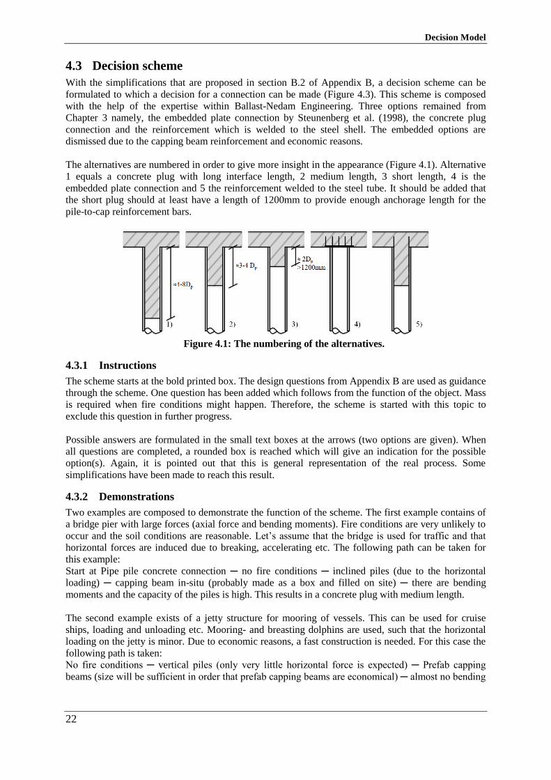
The alternatives are numbered in order to give more insight in the appearance (Figure 4.1). Alternative
1 equals a concrete plug with long interface length, 2 medium length, 3 short length, 4 is the
embedded plate connection and 5 the reinforcement welded to the steel tube. It should be added that
the short plug should at least have a length of 1200mm to provide enough anchorage length for the
pile-to-cap reinforcement bars.
Figure 4.1: The numbering of the alternatives.
4.3.1 Instructions
The scheme starts at the bold printed box. The design questions from Appendix B are used as guidance
through the scheme. One question has been added which follows from the function of the object. Mass
is required when fire conditions might happen. Therefore, the scheme is started with this topic to
exclude this question in further progress.
Possible answers are formulated in the small text boxes at the arrows (two options are given). When
all questions are completed, a rounded box is reached which will give an indication for the possible
option(s). Again, it is pointed out that this is general representation of the real process. Some
simplifications have been made to reach this result.
4.3.2 Demonstrations
Two examples are composed to demonstrate the function of the scheme. The first example contains of
a bridge pier with large forces (axial force and bending moments). Fire conditions are very unlikely to
occur and the soil conditions are reasonable. Let’s assume that the bridge is used for traffic and that
horizontal forces are induced due to breaking, accelerating etc. The following path can be taken for
this example:
Start at Pipe pile concrete connection ─ no fire conditions ─ inclined piles (due to the horizontal
loading) ─ capping beam in-situ (probably made as a box and filled on site) ─ there are bending
moments and the capacity of the piles is high. This results in a concrete plug with medium length.
The second example exists of a jetty structure for mooring of vessels. This can be used for cruise
ships, loading and unloading etc. Mooring- and breasting dolphins are used, such that the horizontal
loading on the jetty is minor. Due to economic reasons, a fast construction is needed. For this case the
following path is taken:
No fire conditions ─ vertical piles (only very little horizontal force is expected) ─ Prefab capping
beams (size will be sufficient in order that prefab capping beams are economical) ─ almost no bending
Decision Model
23
moments ─ fast construction and workshop conditions are sufficient. This results in an embedded plate
connection.
4.3.3 Appearance
Based on the presented scheme, a ratio has been formulated for the appearance chances of each
connection type. Based on experience, the embedded plate is used in approximately 5-10% of all
cases. The reinforcement which is welded to the steel shell is only used rather limited. This seems
logical considering the numbers of steps to be taken during fabrication (this is elaborated in detail in
section 4.4.1.2). In almost all other cases, the concrete plug connection is adopted. This is by far the
most popular alternative.
Trade-off 4.4
The design influences and a general scheme are given for the decision on which connection to adopt.
However, this does not involve aspects like the construction process, the erection time or the costs.
Therefore, research has been done to clarify these so-called trade-off aspects.
4.4.1 Manufacturability
The manufacturability describes the process and the steps which should be taken to complete the
production. It includes transportation, hoisting and lifting, placement difficulties etc. For each
alternative used in Figure 4.3 the complete process is described.
4.4.1.1 Concrete plug
The concrete plug can be made in two ways depending on the plug length. For long plugs the
following method is normally used:
Long plug
At first, the piles are placed according to project descriptions with respect to the capacity and the
allowable pile tip deviations. A working platform is installed (welded onto the piles) and the piles are
flame cut and bevelled to align for further construction. The concrete within the pile is casted in two
stages. The first stage is prior to placement of the capping beam/pile cap. Formwork (steel- or concrete
plate) is lowered into the pile which is connected with hooks to the top of the pile. The reinforcement
cage is positioned within the pile and the first part of the plug is casted (Figure 4.2). A length of 40
times the reinforcement bar diameter below the pile tip remains hollow. This space accounts for the
anchorage length of the pile-to-cap reinforcement.
Figure 4.2: Casting of the first part of the concrete plug.
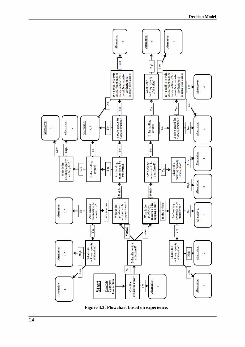
Decision Model
24
Figure 4.3: Flowchart based on experience.
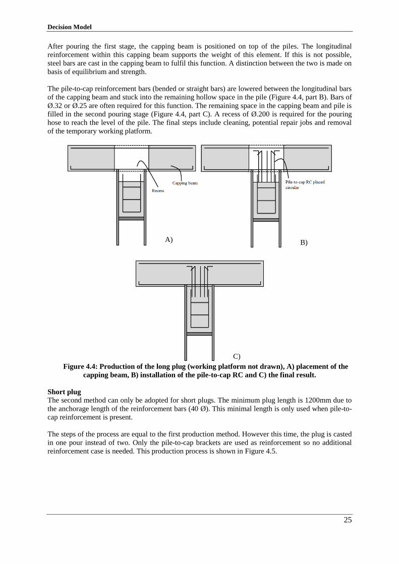
Decision Model
25
After pouring the first stage, the capping beam is positioned on top of the piles. The longitudinal
reinforcement within this capping beam supports the weight of this element. If this is not possible,
steel bars are cast in the capping beam to fulfil this function. A distinction between the two is made on
basis of equilibrium and strength.
The pile-to-cap reinforcement bars (bended or straight bars) are lowered between the longitudinal bars
of the capping beam and stuck into the remaining hollow space in the pile (Figure 4.4, part B). Bars of
Ø.32 or Ø.25 are often required for this function. The remaining space in the capping beam and pile is
filled in the second pouring stage (Figure 4.4, part C). A recess of Ø.200 is required for the pouring
hose to reach the level of the pile. The final steps include cleaning, potential repair jobs and removal
of the temporary working platform.
Figure 4.4: Production of the long plug (working platform not drawn), A) placement of the
capping beam, B) installation of the pile-to-cap RC and C) the final result.
Short plug
The second method can only be adopted for short plugs. The minimum plug length is 1200mm due to
the anchorage length of the reinforcement bars (40 Ø). This minimal length is only used when pile-to-
cap reinforcement is present.
The steps of the process are equal to the first production method. However this time, the plug is casted
in one pour instead of two. Only the pile-to-cap brackets are used as reinforcement so no additional
reinforcement case is needed. This production process is shown in Figure 4.5.
A) B)
C)
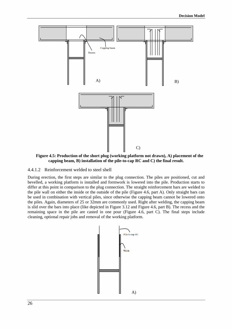
Decision Model
26
Figure 4.5: Production of the short plug (working platform not drawn), A) placement of the
capping beam, B) installation of the pile-to-cap RC and C) the final result.
4.4.1.2 Reinforcement welded to steel shell
During erection, the first steps are similar to the plug connection. The piles are positioned, cut and
bevelled, a working platform is installed and formwork is lowered into the pile. Production starts to
differ at this point in comparison to the plug connection. The straight reinforcement bars are welded to
the pile wall on either the inside or the outside of the pile (Figure 4.6, part A). Only straight bars can
be used in combination with vertical piles, since otherwise the capping beam cannot be lowered onto
the piles. Again, diameters of 25 or 32mm are commonly used. Right after welding, the capping beam
is slid over the bars into place (like depicted in Figure 3.12 and Figure 4.6, part B). The recess and the
remaining space in the pile are casted in one pour (Figure 4.6, part C). The final steps include
cleaning, optional repair jobs and removal of the working platform.
A)
A) B)
C)
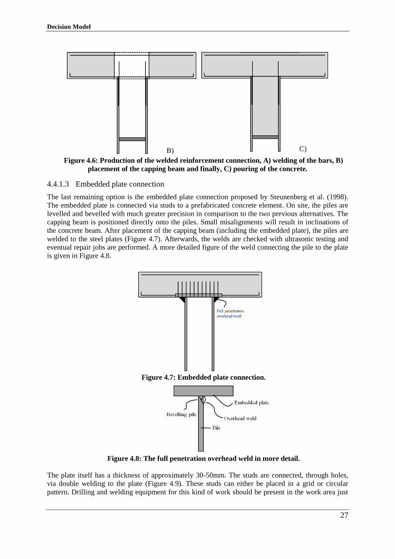
Decision Model
27
Figure 4.6: Production of the welded reinforcement connection, A) welding of the bars, B)
placement of the capping beam and finally, C) pouring of the concrete.
4.4.1.3 Embedded plate connection
The last remaining option is the embedded plate connection proposed by Steunenberg et al. (1998).
The embedded plate is connected via studs to a prefabricated concrete element. On site, the piles are
levelled and bevelled with much greater precision in comparison to the two previous alternatives. The
capping beam is positioned directly onto the piles. Small misalignments will result in inclinations of
the concrete beam. After placement of the capping beam (including the embedded plate), the piles are
welded to the steel plates (Figure 4.7). Afterwards, the welds are checked with ultrasonic testing and
eventual repair jobs are performed. A more detailed figure of the weld connecting the pile to the plate
is given in Figure 4.8.
Figure 4.7: Embedded plate connection.
Figure 4.8: The full penetration overhead weld in more detail.
The plate itself has a thickness of approximately 30-50mm. The studs are connected, through holes,
via double welding to the plate (Figure 4.9). These studs can either be placed in a grid or circular
pattern. Drilling and welding equipment for this kind of work should be present in the work area just
B) C)
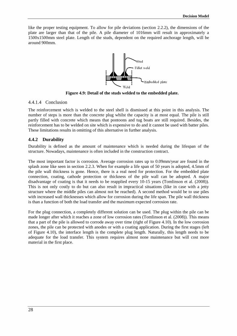
Decision Model
28
like the proper testing equipment. To allow for pile deviations (section 2.2.2), the dimensions of the
plate are larger than that of the pile. A pile diameter of 1016mm will result in approximately a
1500x1500mm steel plate. Length of the studs, dependent on the required anchorage length, will be
around 900mm.
Figure 4.9: Detail of the studs welded to the embedded plate.
4.4.1.4 Conclusion
The reinforcement which is welded to the steel shell is dismissed at this point in this analysis. The
number of steps is more than the concrete plug whilst the capacity is at most equal. The pile is still
partly filled with concrete which means that pontoons and tug boats are still required. Besides, the
reinforcement has to be welded on site which is expensive to do and it cannot be used with batter piles.
These limitations results in omitting of this alternative in further analysis.
4.4.2 Durability
Durability is defined as the amount of maintenance which is needed during the lifespan of the
structure. Nowadays, maintenance is often included in the construction contract.
The most important factor is corrosion. Average corrosion rates up to 0.09mm/year are found in the
splash zone like seen in section 2.2.3. When for example a life span of 50 years is adopted, 4.5mm of
the pile wall thickness is gone. Hence, there is a real need for protection. For the embedded plate
connection, coating, cathode protection or thickness of the pile wall can be adopted. A major
disadvantage of coating is that it needs to be reapplied every 10-15 years (Tomlinson et al. (2008)).
This is not only costly to do but can also result in impractical situations (like in case with a jetty
structure where the middle piles can almost not be reached). A second method would be to use piles
with increased wall thicknesses which allow for corrosion during the life span. The pile wall thickness
is than a function of both the load transfer and the maximum expected corrosion rate.
For the plug connection, a completely different solution can be used. The plug within the pile can be
made longer after which it reaches a zone of low corrosion rates (Tomlinson et al. (2008)). This means
that a part of the pile is allowed to corrode away over time (right of Figure 4.10). In the low corrosion
zones, the pile can be protected with anodes or with a coating application. During the first stages (left
of Figure 4.10), the interface length is the complete plug length. Naturally, this length needs to be
adequate for the load transfer. This system requires almost none maintenance but will cost more
material in the first place.
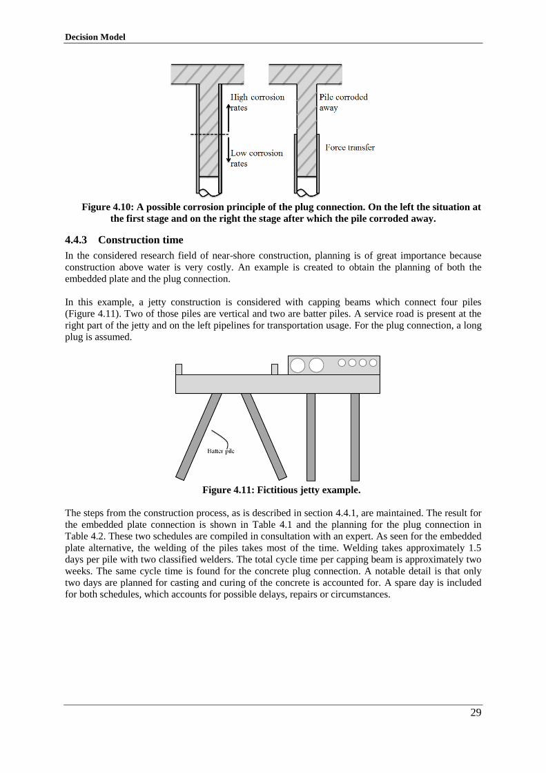
Decision Model
29
Figure 4.10: A possible corrosion principle of the plug connection. On the left the situation at
the first stage and on the right the stage after which the pile corroded away.
4.4.3 Construction time
In the considered research field of near-shore construction, planning is of great importance because
construction above water is very costly. An example is created to obtain the planning of both the
embedded plate and the plug connection.
In this example, a jetty construction is considered with capping beams which connect four piles
(Figure 4.11). Two of those piles are vertical and two are batter piles. A service road is present at the
right part of the jetty and on the left pipelines for transportation usage. For the plug connection, a long
plug is assumed.
Figure 4.11: Fictitious jetty example.
The steps from the construction process, as is described in section 4.4.1, are maintained. The result for
the embedded plate connection is shown in Table 4.1 and the planning for the plug connection in
Table 4.2. These two schedules are compiled in consultation with an expert. As seen for the embedded
plate alternative, the welding of the piles takes most of the time. Welding takes approximately 1.5
days per pile with two classified welders. The total cycle time per capping beam is approximately two
weeks. The same cycle time is found for the concrete plug connection. A notable detail is that only
two days are planned for casting and curing of the concrete is accounted for. A spare day is included
for both schedules, which accounts for possible delays, repairs or circumstances.
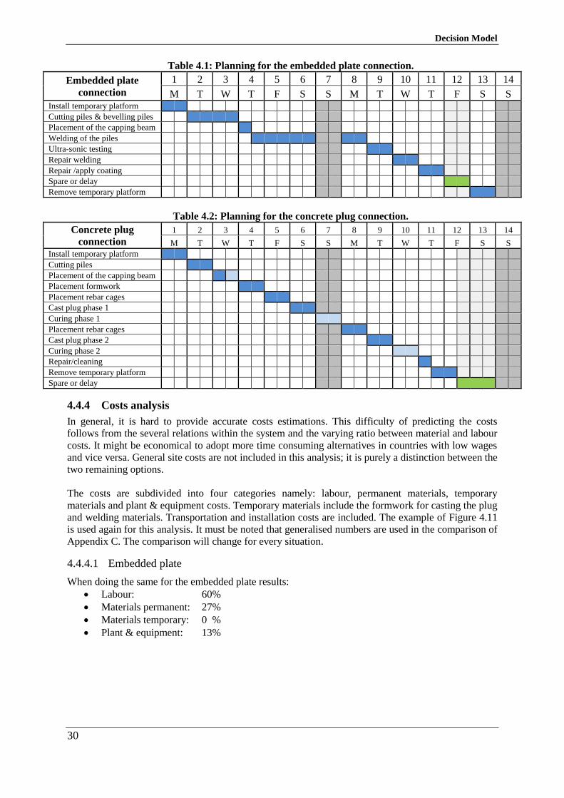
Decision Model
30
Table 4.1: Planning for the embedded plate connection.
Embedded plate
connection
1 2 3 4 5 6 7 8 9 10 11 12 13 14
M T W T F S S M T W T F S S Install temporary platform Cutting piles & bevelling piles Placement of the capping beam Welding of the piles Ultra-sonic testing Repair welding Repair /apply coating Spare or delay Remove temporary platform
Table 4.2: Planning for the concrete plug connection.
Concrete plug
connection
1 2 3 4 5 6 7 8 9 10 11 12 13 14
M T W T F S S M T W T F S S
Install temporary platform Cutting piles Placement of the capping beam Placement formwork Placement rebar cages Cast plug phase 1 Curing phase 1 Placement rebar cages Cast plug phase 2 Curing phase 2 Repair/cleaning Remove temporary platform Spare or delay
4.4.4 Costs analysis
In general, it is hard to provide accurate costs estimations. This difficulty of predicting the costs
follows from the several relations within the system and the varying ratio between material and labour
costs. It might be economical to adopt more time consuming alternatives in countries with low wages
and vice versa. General site costs are not included in this analysis; it is purely a distinction between the
two remaining options.
The costs are subdivided into four categories namely: labour, permanent materials, temporary
materials and plant & equipment costs. Temporary materials include the formwork for casting the plug
and welding materials. Transportation and installation costs are included. The example of Figure 4.11
is used again for this analysis. It must be noted that generalised numbers are used in the comparison of
Appendix C. The comparison will change for every situation.
4.4.4.1 Embedded plate
When doing the same for the embedded plate results:
Labour: 60%
Materials permanent: 27%
Materials temporary: 0 %
Plant & equipment: 13%
Decision Model
31
4.4.4.2 Plug connection
For the plug connection, the following partition is found:
Labour: 6%
Materials permanent: 65%
Materials temporary: 17%
Plant & equipment: 12%
4.4.4.3 Mutual differences
When comparing the plug connection to the embedded plate connection, the plate is around 20-30%
more expensive. The reason is the amount of required manual labour just to make the plate and
perform the welding. Testing is required and coating is required which needs to be reapplied every 10
years (Tomlinson et al. (2008)). The plug connection is relative simple to make since only few
specialized operations are required.
Conclusion 4.5
A general decision scheme is proposed based on the influential aspects. These aspects are subdivided
into a number of decisions to make. These are the construction method of the capping beam, the
construction speed, the function and the capacity of the piles.
Generally seen, the concrete plug is the most suitable solution for the design issue. This is due to the
fact that this connection is cheaper in comparison to the embedded plate connection, the production is
relatively simple and the producing time is comparable with the embedded plate connection. Only in
some situations (determined by local conditions) the embedded plate is more favourable, since it is
constructed in a different manner. Thus from eight possible options, the concrete plug connection will
be examined in more detail in the following chapters.

Decision Model
32
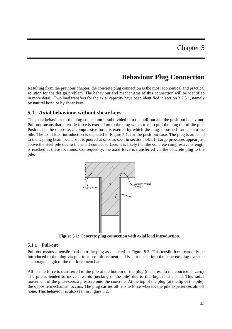
33
Chapter 5
5. Behaviour Plug Connection
Resulting from the previous chapter, the concrete plug connection is the most economical and practical
solution for the design problem. The behaviour and mechanisms of this connection will be identified
in more detail. Two load transfers for the axial capacity have been identified in section 3.2.3.1, namely
by natural bond or by shear keys.
Axial behaviour without shear keys 5.1
The axial behaviour of the plug connection is subdivided into the pull-out and the push-out behaviour.
Pull-out means that a tensile force is exerted on to the plug which tries to pull the plug out of the pile.
Push-out is the opposite; a compressive force is exerted by which the plug is pushed further into the
pile. The axial load introduction is depicted in Figure 5.1, for the push-out case. The plug is attached
to the capping beam because it is poured at once as seen in section 4.4.1.1. Large pressures appear just
above the steel pile due to the small contact surface. It is likely that the concrete compressive strength
is reached at these locations. Consequently, the axial force is transferred via the concrete plug to the
pile.
Figure 5.1: Concrete plug connection with axial load introduction.
5.1.1 Pull-out
Pull-out means a tensile load onto the plug as depicted in Figure 5.2. This tensile force can only be
introduced to the plug via pile-to-cap reinforcement and is introduced into the concrete plug over the
anchorage length of the reinforcement bars.
All tensile force is transferred to the pile at the bottom of the plug (the stress in the concrete is zero).
The pile is tended to move inwards (necking of the pile) due to this high tensile load. This radial
movement of the pile exerts a pressure onto the concrete. At the top of the plug (at the tip of the pile),
the opposite mechanism occurs. The plug carries all tensile force whereas the pile experiences almost
none. This behaviour is also seen in Figure 5.2.
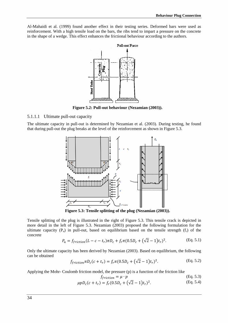
Behaviour Plug Connection
34
Al-Mahaidi et al. (1999) found another effect in their testing series. Deformed bars were used as
reinforcement. With a high tensile load on the bars, the ribs tend to impart a pressure on the concrete
in the shape of a wedge. This effect enhances the frictional behaviour according to the authors.
Figure 5.2: Pull-out behaviour (Nezamian (2003)).
5.1.1.1 Ultimate pull-out capacity
The ultimate capacity in pull-out is determined by Nezamian et al. (2003). During testing, he found
that during pull-out the plug breaks at the level of the reinforcement as shown in Figure 5.3.
Figure 5.3: Tensile splitting of the plug (Nezamian (2003)).
Tensile splitting of the plug is illustrated in the right of Figure 5.3. This tensile crack is depicted in
more detail in the left of Figure 5.3. Nezamian (2003) proposed the following formulation for the
ultimate capacity (Pu) in pull-out, based on equilibrium based on the tensile strength (fr) of the
concrete
𝑃𝑢 = 𝑓𝑓𝑟𝑖𝑐𝑡𝑖𝑜𝑛(𝐿 − 𝑐 − 𝑡𝑟)𝜋𝐷𝑐 + 𝑓𝑟𝜋(0.5𝐷𝑐 + (√2 − 1)𝑡𝑟)2. (Eq. 5.1)
Only the ultimate capacity has been derived by Nezamian (2003). Based on equilibrium, the following
can be obtained
𝑓𝑓𝑟𝑖𝑐𝑡𝑖𝑜𝑛𝜋𝐷𝑐(𝑐 + 𝑡𝑟) = 𝑓𝑟𝜋(0.5𝐷𝑐 + (√2 − 1)𝑡𝑟)2. (Eq. 5.2)
Applying the Mohr- Coulomb friction model, the pressure (p) is a function of the friction like
𝑓𝑓𝑟𝑖𝑐𝑡𝑖𝑜𝑛 = 𝜇 ∙ 𝑝 (Eq. 5.3)
𝜇𝑝𝐷𝑐(𝑐 + 𝑡𝑟) = 𝑓𝑟(0.5𝐷𝑐 + (√2 − 1)𝑡𝑟)2. (Eq. 5.4)
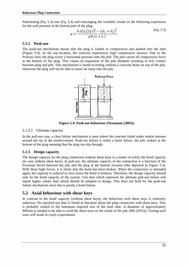
Behaviour Plug Connection
35
Substituting (Eq. 5.3) into (Eq. 5.4) and rearranging the variables results in the following expression
for the wall pressure at the bottom part of the plug.
𝑝 =
0.25𝑓𝑟(2(√2 − 1)𝑡𝑟 + 𝐷𝑐)2
𝜇𝐷𝑐(𝑐 + 𝑡𝑟).
(Eq. 5.5)
5.1.2 Push-out
The push-out mechanism means that the plug is loaded in compression and pushed into the tube
(Figure 5.4). At the top location, the concrete experiences high compressive stresses. Due to the
Poisson ratio, the plug exerts a horizontal pressure onto the pile. The pile carries all compressive force
at the bottom of the plug. This causes an expansion of the pile diameter resulting in low contact
between plug and pile. This mechanism is found in testing without a concrete beam on top of the pile,
otherwise the plug will not be able to move far away into the pile.
Figure 5.4: Push-out behaviour (Nezamian (2003)).
5.1.2.1 Ultimate capacity
In the pull-out case, a clear failure mechanism is seen where the concrete failed under tensile stresses
around the tip of the reinforcement. Push-out failure is really a bond failure, the pile widens at the
bottom of the plug meaning that the plug can slip through.
5.1.3 Design capacity
The design capacity for the plug connection without shear keys is a matter of solely the bond capacity
(in case without shear keys). In pull-out, the ultimate capacity of the connection is a function of the
frictional forces between the pile and the plug at the bottom location (like depicted in Figure 5.3).
With these high forces, it is likely that the bond has been broken. When the connection is unloaded
again, the capacity is reduced to zero (since the bond is broken). Therefore, the design capacity should
only be the bond capacity of the system. Test data which represent the ultimate pull-out failure will
report higher values than which should be adopted in design. This does not hold for the push-out
failure mechanism since this is purely a bond failure.
Axial behaviour with shear keys 5.2
In contrast to the bond capacity (without shear keys), the behaviour with shear keys is relatively
unknown. No reported test data is found in literature about the plug connection with shear keys. This
is probably related to the minimum required size of the steel tube. A diameter of approximately
900mm is needed to be able to weld the shear keys on the inside of the pile (BN (2015)). Testing such
sizes will result in costly experiments.
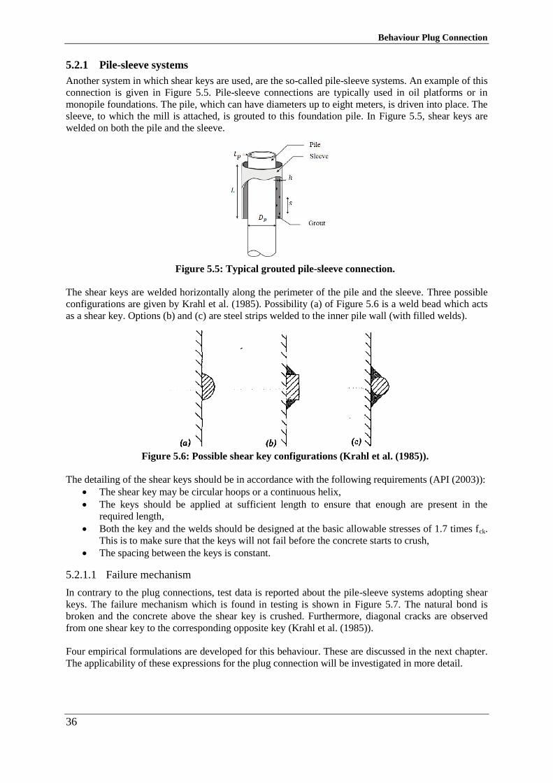
Behaviour Plug Connection
36
5.2.1 Pile-sleeve systems
Another system in which shear keys are used, are the so-called pile-sleeve systems. An example of this
connection is given in Figure 5.5. Pile-sleeve connections are typically used in oil platforms or in
monopile foundations. The pile, which can have diameters up to eight meters, is driven into place. The
sleeve, to which the mill is attached, is grouted to this foundation pile. In Figure 5.5, shear keys are
welded on both the pile and the sleeve.
Figure 5.5: Typical grouted pile-sleeve connection.
The shear keys are welded horizontally along the perimeter of the pile and the sleeve. Three possible
configurations are given by Krahl et al. (1985). Possibility (a) of Figure 5.6 is a weld bead which acts
as a shear key. Options (b) and (c) are steel strips welded to the inner pile wall (with filled welds).
Figure 5.6: Possible shear key configurations (Krahl et al. (1985)).
The detailing of the shear keys should be in accordance with the following requirements (API (2003)):
The shear key may be circular hoops or a continuous helix,
The keys should be applied at sufficient length to ensure that enough are present in the
required length,
Both the key and the welds should be designed at the basic allowable stresses of 1.7 times fck.
This is to make sure that the keys will not fail before the concrete starts to crush,
The spacing between the keys is constant.
5.2.1.1 Failure mechanism
In contrary to the plug connections, test data is reported about the pile-sleeve systems adopting shear
keys. The failure mechanism which is found in testing is shown in Figure 5.7. The natural bond is
broken and the concrete above the shear key is crushed. Furthermore, diagonal cracks are observed
from one shear key to the corresponding opposite key (Krahl et al. (1985)).
Four empirical formulations are developed for this behaviour. These are discussed in the next chapter.
The applicability of these expressions for the plug connection will be investigated in more detail.
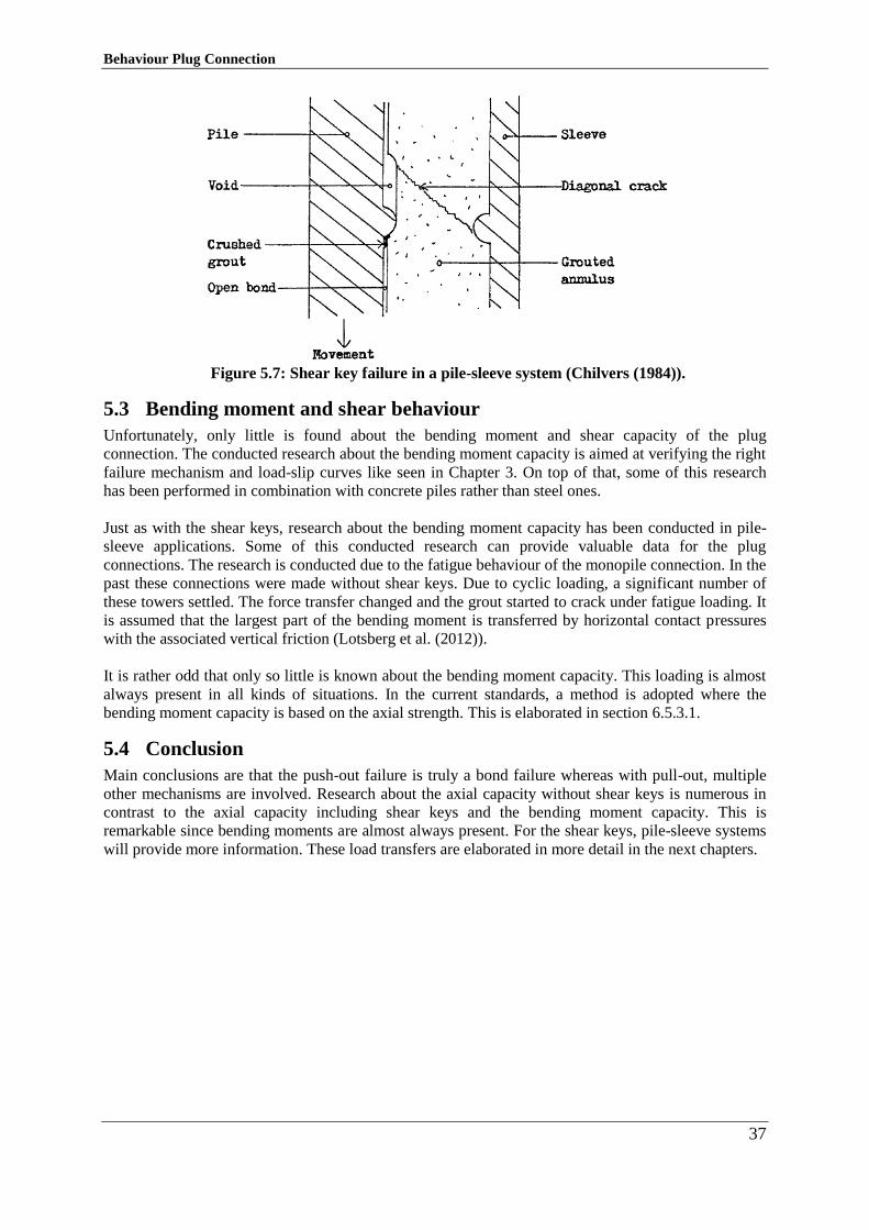
Behaviour Plug Connection
37
Figure 5.7: Shear key failure in a pile-sleeve system (Chilvers (1984)).
Bending moment and shear behaviour 5.3
Unfortunately, only little is found about the bending moment and shear capacity of the plug
connection. The conducted research about the bending moment capacity is aimed at verifying the right
failure mechanism and load-slip curves like seen in Chapter 3. On top of that, some of this research
has been performed in combination with concrete piles rather than steel ones.
Just as with the shear keys, research about the bending moment capacity has been conducted in pile-
sleeve applications. Some of this conducted research can provide valuable data for the plug
connections. The research is conducted due to the fatigue behaviour of the monopile connection. In the
past these connections were made without shear keys. Due to cyclic loading, a significant number of
these towers settled. The force transfer changed and the grout started to crack under fatigue loading. It
is assumed that the largest part of the bending moment is transferred by horizontal contact pressures
with the associated vertical friction (Lotsberg et al. (2012)).
It is rather odd that only so little is known about the bending moment capacity. This loading is almost
always present in all kinds of situations. In the current standards, a method is adopted where the
bending moment capacity is based on the axial strength. This is elaborated in section 6.5.3.1.
Conclusion 5.4
Main conclusions are that the push-out failure is truly a bond failure whereas with pull-out, multiple
other mechanisms are involved. Research about the axial capacity without shear keys is numerous in
contrast to the axial capacity including shear keys and the bending moment capacity. This is
remarkable since bending moments are almost always present. For the shear keys, pile-sleeve systems
will provide more information. These load transfers are elaborated in more detail in the next chapters.

Behaviour Plug Connection
38
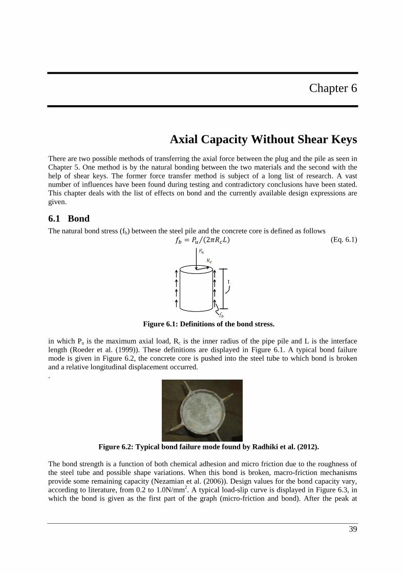
39
Chapter 6
6. Axial Capacity Without Shear Keys
There are two possible methods of transferring the axial force between the plug and the pile as seen in
Chapter 5. One method is by the natural bonding between the two materials and the second with the
help of shear keys. The former force transfer method is subject of a long list of research. A vast
number of influences have been found during testing and contradictory conclusions have been stated.
This chapter deals with the list of effects on bond and the currently available design expressions are
given.
Bond 6.1
The natural bond stress (fb) between the steel pile and the concrete core is defined as follows
𝑓𝑏 = 𝑃𝑢 (2𝜋𝑅𝑐𝐿)⁄ (Eq. 6.1)
Figure 6.1: Definitions of the bond stress.
in which Pu is the maximum axial load, Rc is the inner radius of the pipe pile and L is the interface
length (Roeder et al. (1999)). These definitions are displayed in Figure 6.1. A typical bond failure
mode is given in Figure 6.2, the concrete core is pushed into the steel tube to which bond is broken
and a relative longitudinal displacement occurred.
.
Figure 6.2: Typical bond failure mode found by Radhiki et al. (2012).
The bond strength is a function of both chemical adhesion and micro friction due to the roughness of
the steel tube and possible shape variations. When this bond is broken, macro-friction mechanisms
provide some remaining capacity (Nezamian et al. (2006)). Design values for the bond capacity vary,
according to literature, from 0.2 to 1.0N/mm2. A typical load-slip curve is displayed in Figure 6.3, in
which the bond is given as the first part of the graph (micro-friction and bond). After the peak at
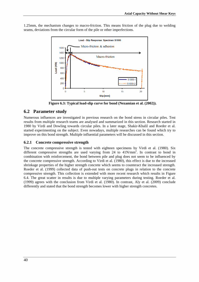
Axial Capacity Without Shear Keys
40
1.25mm, the mechanism changes to macro-friction. This means friction of the plug due to welding
seams, deviations from the circular form of the pile or other imperfections.
Figure 6.3: Typical load-slip curve for bond (Nezamian et al. (2002)).
Parameter study 6.2
Numerous influences are investigated in previous research on the bond stress in circular piles. Test
results from multiple research teams are analysed and summarized in this section. Research started in
1980 by Virdi and Dowling towards circular piles. In a later stage, Shakir-Khalil and Roeder et al.
started experimenting on the subject. Even nowadays, multiple researches can be found which try to
improve on this bond strength. Multiple influential parameters will be discussed in this section.
6.2.1 Concrete compressive strength
The concrete compressive strength is tested with eighteen specimens by Virdi et al. (1980). Six
different compressive strengths are used varying from 24 to 41N/mm2. In contrast to bond in
combination with reinforcement, the bond between pile and plug does not seem to be influenced by
the concrete compressive strength. According to Virdi et al. (1980), this effect is due to the increased
shrinkage properties of the higher strength concrete which seems to counteract the increased strength.
Roeder et al. (1999) collected data of push-out tests on concrete plugs in relation to the concrete
compressive strength. This collection is extended with more recent research which results in Figure
6.4. The great scatter in results is due to multiple varying parameters during testing. Roeder et al.
(1999) agrees with the conclusion from Virdi et al. (1980). In contrast, Aly et al. (2009) conclude
differently and stated that the bond strength becomes lower with higher strength concretes.
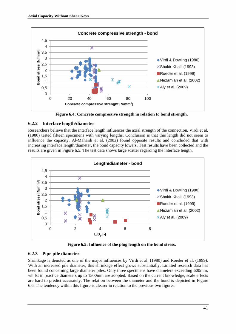
Axial Capacity Without Shear Keys
41
Figure 6.4: Concrete compressive strength in relation to bond strength.
6.2.2 Interface length/diameter
Researchers believe that the interface length influences the axial strength of the connection. Virdi et al.
(1980) tested fifteen specimens with varying lengths. Conclusion is that this length did not seem to
influence the capacity. Al-Mahaidi et al. (2002) found opposite results and concluded that with
increasing interface length/diameter, the bond capacity lowers. Test results have been collected and the
results are given in Figure 6.5. The test data shows large scatter regarding the interface length.
Figure 6.5: Influence of the plug length on the bond stress.
6.2.3 Pipe pile diameter
Shrinkage is denoted as one of the major influences by Virdi et al. (1980) and Roeder et al. (1999).
With an increased pile diameter, this shrinkage effect grows substantially. Limited research data has
been found concerning large diameter piles. Only three specimens have diameters exceeding 600mm,
whilst in practice diameters up to 1500mm are adopted. Based on the current knowledge, scale effects
are hard to predict accurately. The relation between the diameter and the bond is depicted in Figure
6.6. The tendency within this figure is clearer in relation to the previous two figures.
0
0,5
1
1,5
2
2,5
3
3,5
4
4,5
0 20 40 60 80 100
Bo
nd
str
es
s [
N/m
m2]
Concrete compressive strenght [N/mm2]
Concrete compressive strength - bond
Virdi & Dowling (1980)
Shakir-Khalil (1993)
Roeder et al. (1999)
Nezamian et al. (2002)
Aly et al. (2009)
0
0,5
1
1,5
2
2,5
3
3,5
4
4,5
0 2 4 6 8
Bo
nd
str
es
s [
N/m
m2]
L/Dp [-]
Length/diameter - bond
Virdi & Dowling (1980)
Shakir-Khalil (1993)
Roeder et al. (1999)
Nezamian et al. (2002)
Aly et al. (2009)
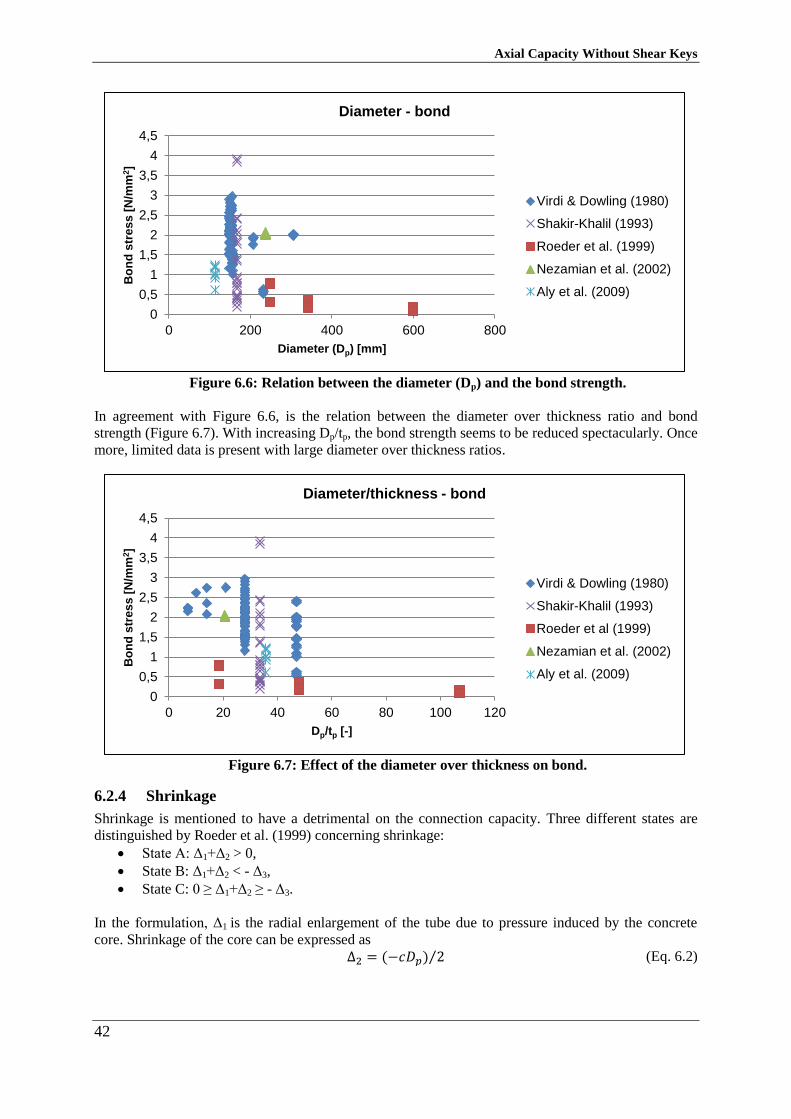
Axial Capacity Without Shear Keys
42
Figure 6.6: Relation between the diameter (Dp) and the bond strength.
In agreement with Figure 6.6, is the relation between the diameter over thickness ratio and bond
strength (Figure 6.7). With increasing Dp/tp, the bond strength seems to be reduced spectacularly. Once
more, limited data is present with large diameter over thickness ratios.
Figure 6.7: Effect of the diameter over thickness on bond.
6.2.4 Shrinkage
Shrinkage is mentioned to have a detrimental on the connection capacity. Three different states are
distinguished by Roeder et al. (1999) concerning shrinkage:
State A: Δ1+Δ2 > 0,
State B: Δ1+Δ2 < - Δ3,
State C: 0 ≥ Δ1+Δ2 ≥ - Δ3.
In the formulation, Δ1 is the radial enlargement of the tube due to pressure induced by the concrete
core. Shrinkage of the core can be expressed as
Δ2 = (−𝑐𝐷𝑝) 2⁄ (Eq. 6.2)
0
0,5
1
1,5
2
2,5
3
3,5
4
4,5
0 200 400 600 800
Bo
nd
str
es
s [
N/m
m2]
Diameter (Dp) [mm]
Diameter - bond
Virdi & Dowling (1980)
Shakir-Khalil (1993)
Roeder et al. (1999)
Nezamian et al. (2002)
Aly et al. (2009)
0
0,5
1
1,5
2
2,5
3
3,5
4
4,5
0 20 40 60 80 100 120
Bo
nd
str
es
s [
N/m
m2]
Dp/tp [-]
Diameter/thickness - bond
Virdi & Dowling (1980)
Shakir-Khalil (1993)
Roeder et al (1999)
Nezamian et al. (2002)
Aly et al. (2009)
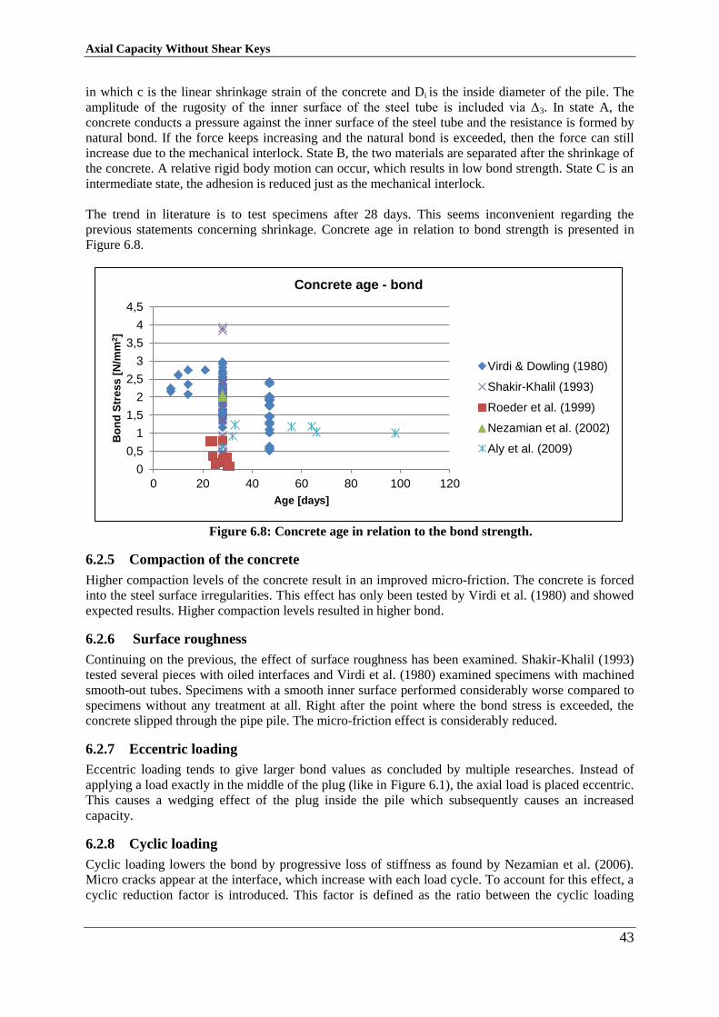
Axial Capacity Without Shear Keys
43
in which c is the linear shrinkage strain of the concrete and Di is the inside diameter of the pile. The
amplitude of the rugosity of the inner surface of the steel tube is included via Δ3. In state A, the
concrete conducts a pressure against the inner surface of the steel tube and the resistance is formed by
natural bond. If the force keeps increasing and the natural bond is exceeded, then the force can still
increase due to the mechanical interlock. State B, the two materials are separated after the shrinkage of
the concrete. A relative rigid body motion can occur, which results in low bond strength. State C is an
intermediate state, the adhesion is reduced just as the mechanical interlock.
The trend in literature is to test specimens after 28 days. This seems inconvenient regarding the
previous statements concerning shrinkage. Concrete age in relation to bond strength is presented in
Figure 6.8.
Figure 6.8: Concrete age in relation to the bond strength.
6.2.5 Compaction of the concrete
Higher compaction levels of the concrete result in an improved micro-friction. The concrete is forced
into the steel surface irregularities. This effect has only been tested by Virdi et al. (1980) and showed
expected results. Higher compaction levels resulted in higher bond.
6.2.6 Surface roughness
Continuing on the previous, the effect of surface roughness has been examined. Shakir-Khalil (1993)
tested several pieces with oiled interfaces and Virdi et al. (1980) examined specimens with machined
smooth-out tubes. Specimens with a smooth inner surface performed considerably worse compared to
specimens without any treatment at all. Right after the point where the bond stress is exceeded, the
concrete slipped through the pipe pile. The micro-friction effect is considerably reduced.
6.2.7 Eccentric loading
Eccentric loading tends to give larger bond values as concluded by multiple researches. Instead of
applying a load exactly in the middle of the plug (like in Figure 6.1), the axial load is placed eccentric.
This causes a wedging effect of the plug inside the pile which subsequently causes an increased
capacity.
6.2.8 Cyclic loading
Cyclic loading lowers the bond by progressive loss of stiffness as found by Nezamian et al. (2006).
Micro cracks appear at the interface, which increase with each load cycle. To account for this effect, a
cyclic reduction factor is introduced. This factor is defined as the ratio between the cyclic loading
0
0,5
1
1,5
2
2,5
3
3,5
4
4,5
0 20 40 60 80 100 120
Bo
nd
Str
es
s [
N/m
m2]
Age [days]
Concrete age - bond
Virdi & Dowling (1980)
Shakir-Khalil (1993)
Roeder et al. (1999)
Nezamian et al. (2002)
Aly et al. (2009)
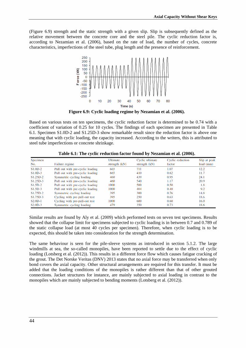
Axial Capacity Without Shear Keys
44
(Figure 6.9) strength and the static strength with a given slip. Slip is subsequently defined as the
relative movement between the concrete core and the steel pile. The cyclic reduction factor is,
according to Nezamian et al. (2006), based on the rate of load, the number of cycles, concrete
characteristics, imperfections of the steel tube, plug length and the presence of reinforcement.
Figure 6.9: Cyclic loading regime by Nezamian et al. (2006).
Based on various tests on ten specimens, the cyclic reduction factor is determined to be 0.74 with a
coefficient of variation of 0.25 for 10 cycles. The findings of each specimen are presented in Table
6.1. Specimen S1.0D-2 and S1.25D-3 show remarkable result since the reduction factor is above one
meaning that with cyclic loading, the capacity increased. According to the writers, this is attributed to
steel tube imperfections or concrete shrinkage.
Table 6.1: The cyclic reduction factor found by Nezamian et al. (2006).
Similar results are found by Aly et al. (2009) which performed tests on seven test specimens. Results
showed that the collapse limit for specimens subjected to cyclic loading is in between 0.7 and 0.789 of
the static collapse load (at most 40 cycles per specimen). Therefore, when cyclic loading is to be
expected, this should be taken into consideration for the strength determination.
The same behaviour is seen for the pile-sleeve systems as introduced in section 5.1.2. The large
windmills at sea, the so-called monopiles, have been reported to settle due to the effect of cyclic
loading (Lotsberg et al. (2012)). This results in a different force flow which causes fatigue cracking of
the grout. The Det Norske Veritas (DNV) 2013 states that no axial force may be transferred when only
bond covers the axial capacity. Other structural arrangements are required for this transfer. It must be
added that the loading conditions of the monopiles is rather different than that of other grouted
connections. Jacket structures for instance, are mainly subjected to axial loading in contrast to the
monopiles which are mainly subjected to bending moments (Lotsberg et al. (2012)).
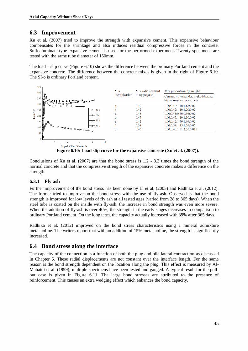
Axial Capacity Without Shear Keys
45
Improvement 6.3
Xu et al. (2007) tried to improve the strength with expansive cement. This expansive behaviour
compensates for the shrinkage and also induces residual compressive forces in the concrete.
Sulfoaluminate-type expansive cement is used for the performed experiment. Twenty specimens are
tested with the same tube diameter of 150mm.
The load – slip curve (Figure 6.10) shows the difference between the ordinary Portland cement and the
expansive concrete. The difference between the concrete mixes is given in the right of Figure 6.10.
The SI-o is ordinary Portland cement.
Figure 6.10: Load slip curve for the expansive concrete (Xu et al. (2007)).
Conclusions of Xu et al. (2007) are that the bond stress is 1.2 - 3.3 times the bond strength of the
normal concrete and that the compressive strength of the expansive concrete makes a difference on the
strength.
6.3.1 Fly ash
Further improvement of the bond stress has been done by Li et al. (2005) and Radhika et al. (2012).
The former tried to improve on the bond stress with the use of fly-ash. Observed is that the bond
strength is improved for low levels of fly ash at all tested ages (varied from 28 to 365 days). When the
steel tube is coated on the inside with fly-ash, the increase in bond strength was even more severe.
When the addition of fly-ash is over 40%, the strength in the early stages decreases in comparison to
ordinary Portland cement. On the long term, the capacity actually increased with 39% after 365 days.
Radhika et al. (2012) improved on the bond stress characteristics using a mineral admixture
metakaoline. The writers report that with an addition of 15% metakaoline, the strength is significantly
increased.
Bond stress along the interface 6.4
The capacity of the connection is a function of both the plug and pile lateral contraction as discussed
in Chapter 5. These radial displacements are not constant over the interface length. For the same
reason is the bond strength dependent on the location along the plug. This effect is measured by Al-
Mahaidi et al. (1999); multiple specimens have been tested and gauged. A typical result for the pull-
out case is given in Figure 6.11. The large bond stresses are attributed to the presence of
reinforcement. This causes an extra wedging effect which enhances the bond capacity.
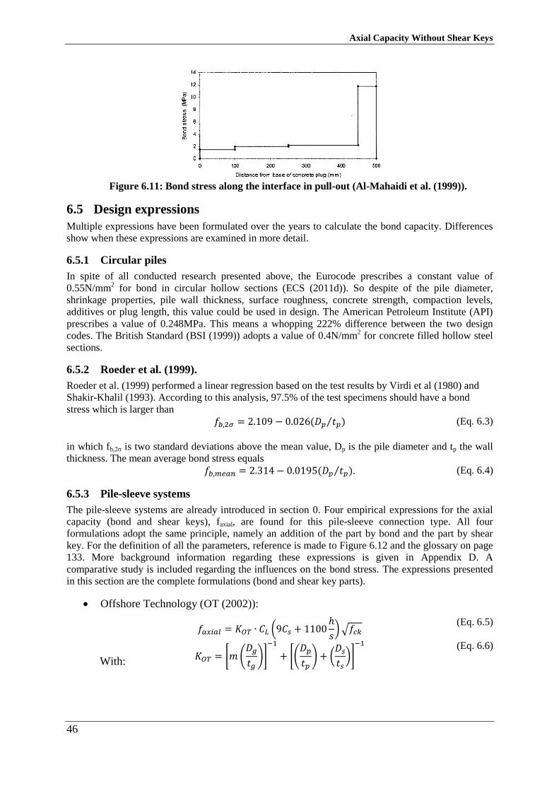
Axial Capacity Without Shear Keys
46
Figure 6.11: Bond stress along the interface in pull-out (Al-Mahaidi et al. (1999)).
Design expressions 6.5
Multiple expressions have been formulated over the years to calculate the bond capacity. Differences
show when these expressions are examined in more detail.
6.5.1 Circular piles
In spite of all conducted research presented above, the Eurocode prescribes a constant value of
0.55N/mm2 for bond in circular hollow sections (ECS (2011d)). So despite of the pile diameter,
shrinkage properties, pile wall thickness, surface roughness, concrete strength, compaction levels,
additives or plug length, this value could be used in design. The American Petroleum Institute (API)
prescribes a value of 0.248MPa. This means a whopping 222% difference between the two design
codes. The British Standard (BSI (1999)) adopts a value of 0.4N/mm2 for concrete filled hollow steel
sections.
6.5.2 Roeder et al. (1999).
Roeder et al. (1999) performed a linear regression based on the test results by Virdi et al (1980) and
Shakir-Khalil (1993). According to this analysis, 97.5% of the test specimens should have a bond
stress which is larger than
𝑓𝑏,2𝜎 = 2.109 − 0.026(𝐷𝑝 𝑡𝑝⁄ ) (Eq. 6.3)
in which fb,2σ is two standard deviations above the mean value, Dp is the pile diameter and tp the wall
thickness. The mean average bond stress equals
𝑓𝑏,𝑚𝑒𝑎𝑛 = 2.314 − 0.0195(𝐷𝑝 𝑡𝑝⁄ ). (Eq. 6.4)
6.5.3 Pile-sleeve systems
The pile-sleeve systems are already introduced in section 0. Four empirical expressions for the axial
capacity (bond and shear keys), faxial, are found for this pile-sleeve connection type. All four
formulations adopt the same principle, namely an addition of the part by bond and the part by shear
key. For the definition of all the parameters, reference is made to Figure 6.12 and the glossary on page
133. More background information regarding these expressions is given in Appendix D. A
comparative study is included regarding the influences on the bond stress. The expressions presented
in this section are the complete formulations (bond and shear key parts).
Offshore Technology (OT (2002)):
With:
𝑓𝑎𝑥𝑖𝑎𝑙 = 𝐾𝑂𝑇 ∙ 𝐶𝐿 (9𝐶𝑠 + 1100ℎ
𝑠)√𝑓𝑐𝑘
𝐾𝑂𝑇 = [𝑚(𝐷𝑔
𝑡𝑔)]
−1
+ [(𝐷𝑝
𝑡𝑝) + (
𝐷𝑠𝑡𝑠)]
−1
(Eq. 6.5)
(Eq. 6.6)
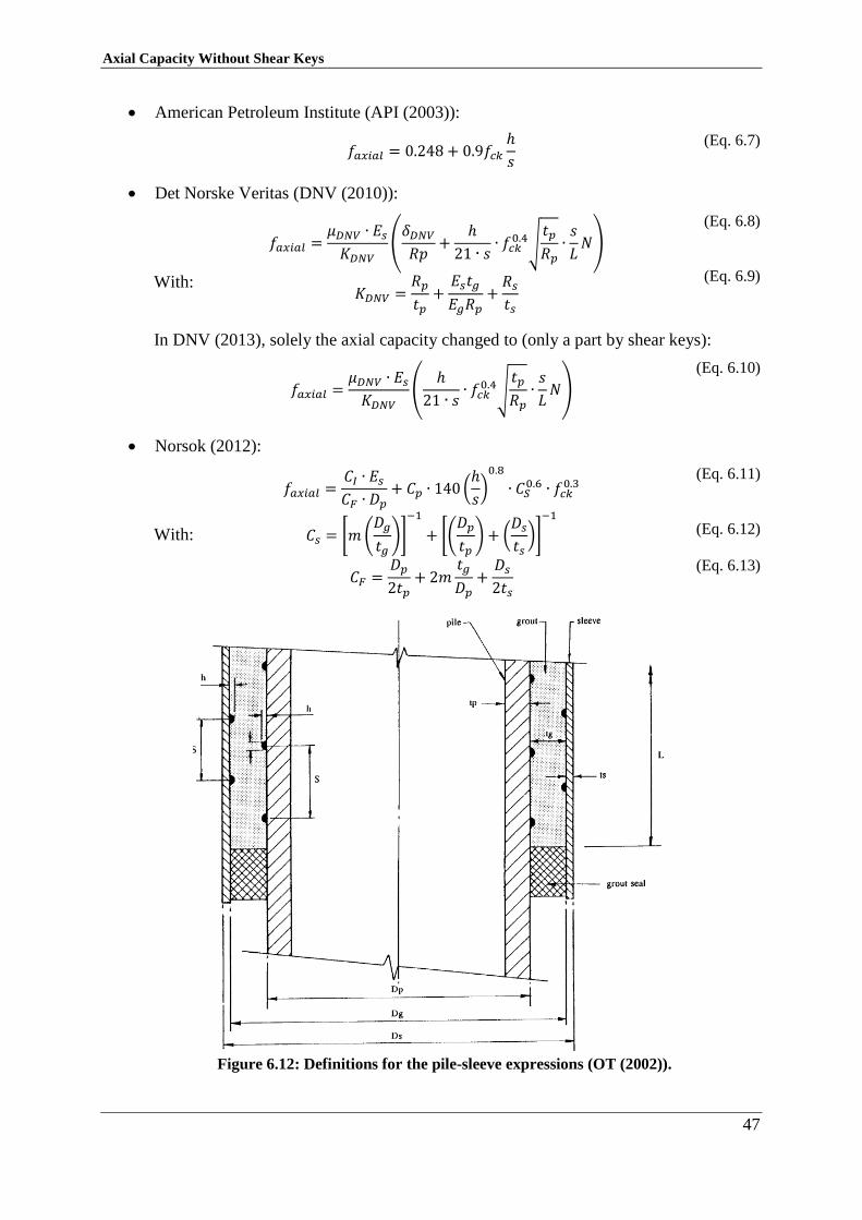
Axial Capacity Without Shear Keys
47
American Petroleum Institute (API (2003)):
𝑓𝑎𝑥𝑖𝑎𝑙 = 0.248 + 0.9𝑓𝑐𝑘
ℎ
𝑠
(Eq. 6.7)
Det Norske Veritas (DNV (2010)):
With:
𝑓𝑎𝑥𝑖𝑎𝑙 =𝜇𝐷𝑁𝑉 ∙ 𝐸𝑠𝐾𝐷𝑁𝑉
(𝛿𝐷𝑁𝑉𝑅𝑝
+ℎ
21 ∙ 𝑠∙ 𝑓𝑐𝑘0.4√
𝑡𝑝𝑅𝑝∙𝑠
𝐿𝑁)
𝐾𝐷𝑁𝑉 =𝑅𝑝
𝑡𝑝+𝐸𝑠𝑡𝑔
𝐸𝑔𝑅𝑝+𝑅𝑠𝑡𝑠
(Eq. 6.8)
(Eq. 6.9)
In DNV (2013), solely the axial capacity changed to (only a part by shear keys):
𝑓𝑎𝑥𝑖𝑎𝑙 =𝜇𝐷𝑁𝑉 ∙ 𝐸𝑠𝐾𝐷𝑁𝑉
(ℎ
21 ∙ 𝑠∙ 𝑓𝑐𝑘0.4√
𝑡𝑝
𝑅𝑝∙𝑠
𝐿𝑁)
(Eq. 6.10)
Norsok (2012):
With:
𝑓𝑎𝑥𝑖𝑎𝑙 =𝐶𝐼 ∙ 𝐸𝑠𝐶𝐹 ∙ 𝐷𝑝
+ 𝐶𝑝 ∙ 140 (ℎ
𝑠)0.8
∙ 𝐶𝑆0.6 ∙ 𝑓𝑐𝑘
0.3
𝐶𝑠 = [𝑚(𝐷𝑔
𝑡𝑔)]
−1
+ [(𝐷𝑝𝑡𝑝) + (
𝐷𝑠𝑡𝑠)]
−1
𝐶𝐹 =𝐷𝑝
2𝑡𝑝+ 2𝑚
𝑡𝑔
𝐷𝑝+𝐷𝑠2𝑡𝑠
(Eq. 6.11)
(Eq. 6.12)
(Eq. 6.13)
Figure 6.12: Definitions for the pile-sleeve expressions (OT (2002)).
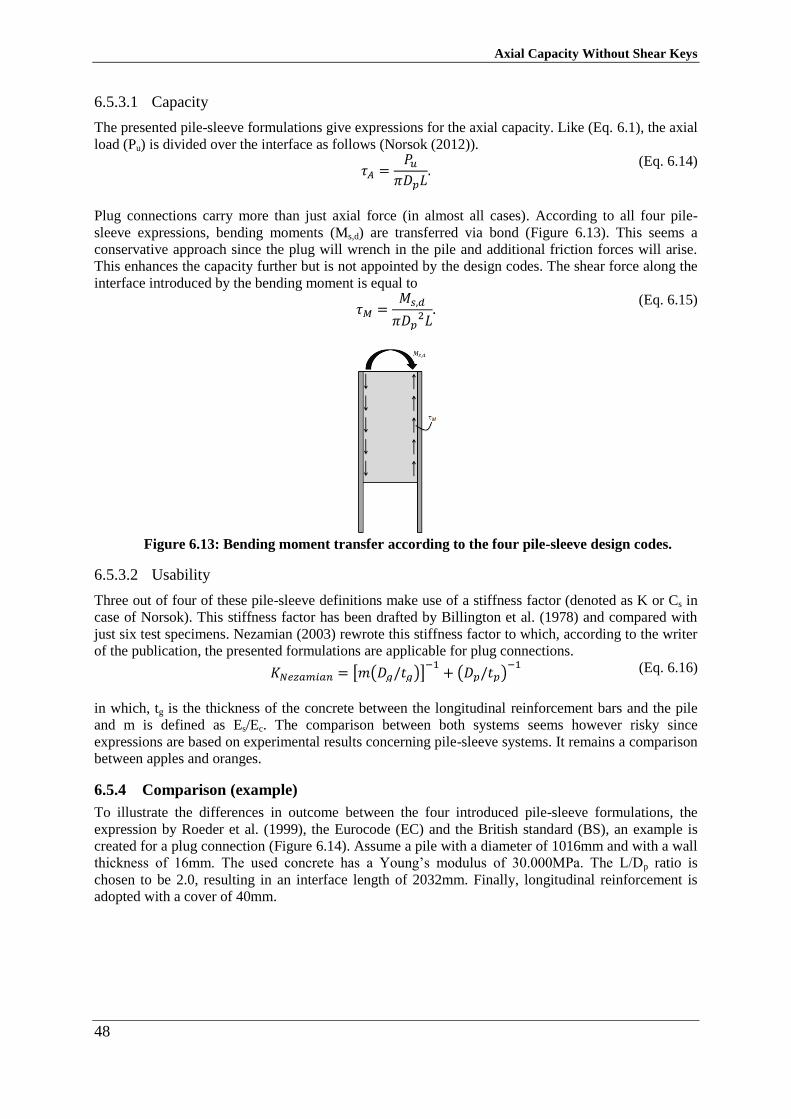
Axial Capacity Without Shear Keys
48
6.5.3.1 Capacity
The presented pile-sleeve formulations give expressions for the axial capacity. Like (Eq. 6.1), the axial
load (Pu) is divided over the interface as follows (Norsok (2012)).
𝜏𝐴 =
𝑃𝑢𝜋𝐷𝑝𝐿
. (Eq. 6.14)
Plug connections carry more than just axial force (in almost all cases). According to all four pile-
sleeve expressions, bending moments (Ms,d) are transferred via bond (Figure 6.13). This seems a
conservative approach since the plug will wrench in the pile and additional friction forces will arise.
This enhances the capacity further but is not appointed by the design codes. The shear force along the
interface introduced by the bending moment is equal to
𝜏𝑀 =
𝑀𝑠,𝑑
𝜋𝐷𝑝2𝐿.
(Eq. 6.15)
Figure 6.13: Bending moment transfer according to the four pile-sleeve design codes.
6.5.3.2 Usability
Three out of four of these pile-sleeve definitions make use of a stiffness factor (denoted as K or Cs in
case of Norsok). This stiffness factor has been drafted by Billington et al. (1978) and compared with
just six test specimens. Nezamian (2003) rewrote this stiffness factor to which, according to the writer
of the publication, the presented formulations are applicable for plug connections.
𝐾𝑁𝑒𝑧𝑎𝑚𝑖𝑎𝑛 = [𝑚(𝐷𝑔/𝑡𝑔)]−1+ (𝐷𝑝/𝑡𝑝)
−1 (Eq. 6.16)
in which, tg is the thickness of the concrete between the longitudinal reinforcement bars and the pile
and m is defined as Es/Ec. The comparison between both systems seems however risky since
expressions are based on experimental results concerning pile-sleeve systems. It remains a comparison
between apples and oranges.
6.5.4 Comparison (example)
To illustrate the differences in outcome between the four introduced pile-sleeve formulations, the
expression by Roeder et al. (1999), the Eurocode (EC) and the British standard (BS), an example is
created for a plug connection (Figure 6.14). Assume a pile with a diameter of 1016mm and with a wall
thickness of 16mm. The used concrete has a Young’s modulus of 30.000MPa. The L/Dp ratio is
chosen to be 2.0, resulting in an interface length of 2032mm. Finally, longitudinal reinforcement is
adopted with a cover of 40mm.
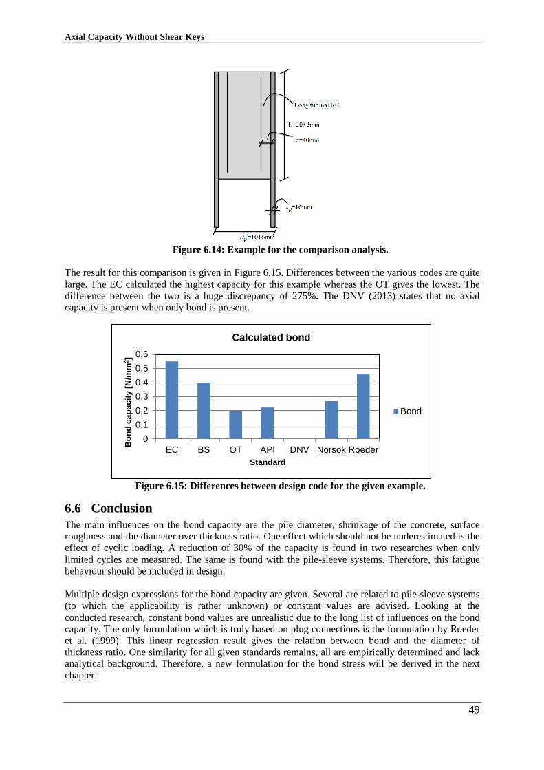
Axial Capacity Without Shear Keys
49
Figure 6.14: Example for the comparison analysis.
The result for this comparison is given in Figure 6.15. Differences between the various codes are quite
large. The EC calculated the highest capacity for this example whereas the OT gives the lowest. The
difference between the two is a huge discrepancy of 275%. The DNV (2013) states that no axial
capacity is present when only bond is present.
Figure 6.15: Differences between design code for the given example.
Conclusion 6.6
The main influences on the bond capacity are the pile diameter, shrinkage of the concrete, surface
roughness and the diameter over thickness ratio. One effect which should not be underestimated is the
effect of cyclic loading. A reduction of 30% of the capacity is found in two researches when only
limited cycles are measured. The same is found with the pile-sleeve systems. Therefore, this fatigue
behaviour should be included in design.
Multiple design expressions for the bond capacity are given. Several are related to pile-sleeve systems
(to which the applicability is rather unknown) or constant values are advised. Looking at the
conducted research, constant bond values are unrealistic due to the long list of influences on the bond
capacity. The only formulation which is truly based on plug connections is the formulation by Roeder
et al. (1999). This linear regression result gives the relation between bond and the diameter of
thickness ratio. One similarity for all given standards remains, all are empirically determined and lack
analytical background. Therefore, a new formulation for the bond stress will be derived in the next
chapter.
0
0,1
0,2
0,3
0,4
0,5
0,6
EC BS OT API DNV Norsok Roeder
Bo
nd
ca
pa
cit
y [
N/m
m2]
Standard
Calculated bond
Bond

Axial Capacity Without Shear Keys
50
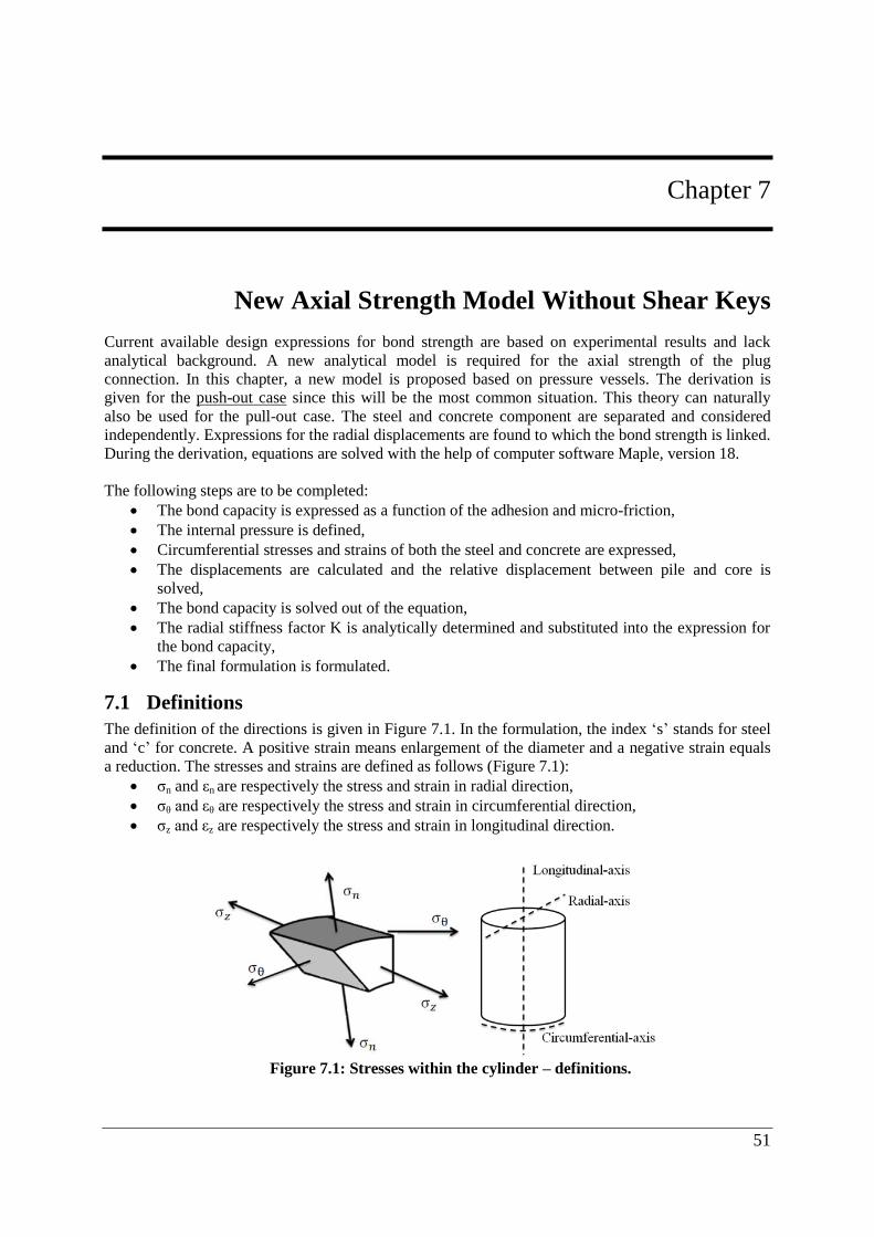
51
Chapter 7
7. New Axial Strength Model Without Shear Keys
Current available design expressions for bond strength are based on experimental results and lack
analytical background. A new analytical model is required for the axial strength of the plug
connection. In this chapter, a new model is proposed based on pressure vessels. The derivation is
given for the push-out case since this will be the most common situation. This theory can naturally
also be used for the pull-out case. The steel and concrete component are separated and considered
independently. Expressions for the radial displacements are found to which the bond strength is linked.
During the derivation, equations are solved with the help of computer software Maple, version 18.
The following steps are to be completed:
The bond capacity is expressed as a function of the adhesion and micro-friction,
The internal pressure is defined,
Circumferential stresses and strains of both the steel and concrete are expressed,
The displacements are calculated and the relative displacement between pile and core is
solved,
The bond capacity is solved out of the equation,
The radial stiffness factor K is analytically determined and substituted into the expression for
the bond capacity,
The final formulation is formulated.
Definitions 7.1
The definition of the directions is given in Figure 7.1. In the formulation, the index ‘s’ stands for steel
and ‘c’ for concrete. A positive strain means enlargement of the diameter and a negative strain equals
a reduction. The stresses and strains are defined as follows (Figure 7.1):
σn and εn are respectively the stress and strain in radial direction,
σθ and εθ are respectively the stress and strain in circumferential direction,
σz and εz are respectively the stress and strain in longitudinal direction.
Figure 7.1: Stresses within the cylinder – definitions.
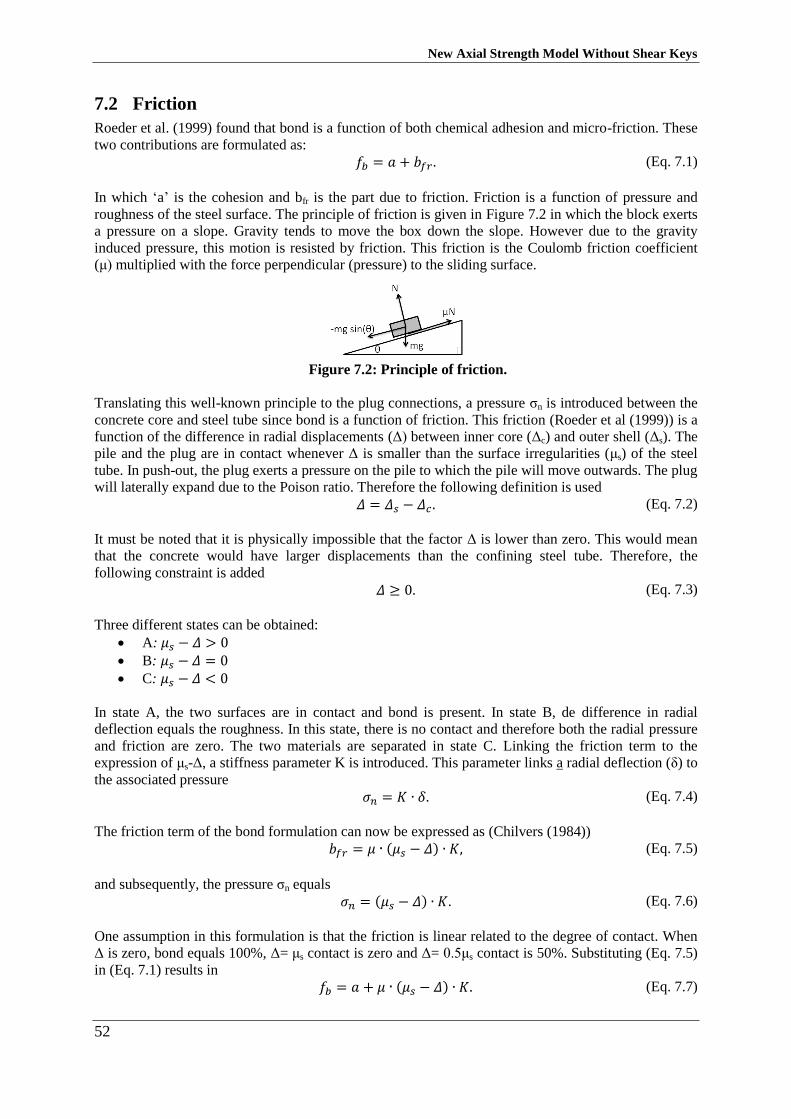
New Axial Strength Model Without Shear Keys
52
Friction 7.2
Roeder et al. (1999) found that bond is a function of both chemical adhesion and micro-friction. These
two contributions are formulated as:
𝑓𝑏 = 𝑎 + 𝑏𝑓𝑟. (Eq. 7.1)
In which ‘a’ is the cohesion and bfr is the part due to friction. Friction is a function of pressure and
roughness of the steel surface. The principle of friction is given in Figure 7.2 in which the block exerts
a pressure on a slope. Gravity tends to move the box down the slope. However due to the gravity
induced pressure, this motion is resisted by friction. This friction is the Coulomb friction coefficient
(μ) multiplied with the force perpendicular (pressure) to the sliding surface.
Figure 7.2: Principle of friction.
Translating this well-known principle to the plug connections, a pressure σn is introduced between the
concrete core and steel tube since bond is a function of friction. This friction (Roeder et al (1999)) is a
function of the difference in radial displacements (Δ) between inner core (Δc) and outer shell (Δs). The
pile and the plug are in contact whenever Δ is smaller than the surface irregularities (μs) of the steel
tube. In push-out, the plug exerts a pressure on the pile to which the pile will move outwards. The plug
will laterally expand due to the Poison ratio. Therefore the following definition is used
𝛥 = 𝛥𝑠 − 𝛥𝑐 . (Eq. 7.2)
It must be noted that it is physically impossible that the factor Δ is lower than zero. This would mean
that the concrete would have larger displacements than the confining steel tube. Therefore, the
following constraint is added
𝛥 ≥ 0. (Eq. 7.3)
Three different states can be obtained:
A: 𝜇𝑠 − 𝛥 > 0
B: 𝜇𝑠 − 𝛥 = 0
C: 𝜇𝑠 − 𝛥 < 0
In state A, the two surfaces are in contact and bond is present. In state B, de difference in radial
deflection equals the roughness. In this state, there is no contact and therefore both the radial pressure
and friction are zero. The two materials are separated in state C. Linking the friction term to the
expression of μs-Δ, a stiffness parameter K is introduced. This parameter links a radial deflection (δ) to
the associated pressure
𝜎𝑛 = 𝐾 ∙ 𝛿. (Eq. 7.4)
The friction term of the bond formulation can now be expressed as (Chilvers (1984))
𝑏𝑓𝑟 = 𝜇 ∙ (𝜇𝑠 − 𝛥) ∙ 𝐾, (Eq. 7.5)
and subsequently, the pressure σn equals
𝜎𝑛 = (𝜇𝑠 − 𝛥) ∙ 𝐾. (Eq. 7.6)
One assumption in this formulation is that the friction is linear related to the degree of contact. When
Δ is zero, bond equals 100%, Δ= μs contact is zero and Δ= 0.5μs contact is 50%. Substituting (Eq. 7.5)
in (Eq. 7.1) results in
𝑓𝑏 = 𝑎 + 𝜇 ∙ (𝜇𝑠 − 𝛥) ∙ 𝐾. (Eq. 7.7)
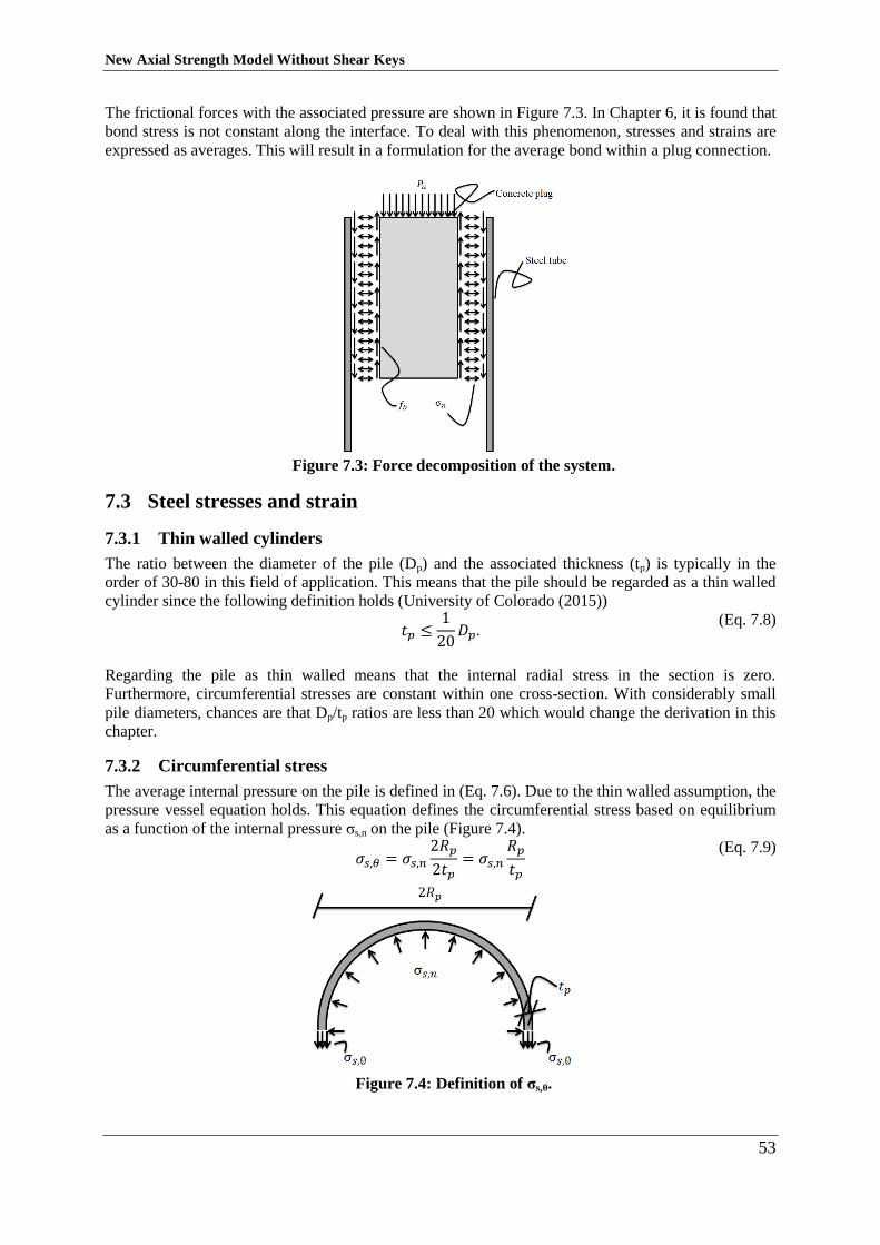
New Axial Strength Model Without Shear Keys
53
The frictional forces with the associated pressure are shown in Figure 7.3. In Chapter 6, it is found that
bond stress is not constant along the interface. To deal with this phenomenon, stresses and strains are
expressed as averages. This will result in a formulation for the average bond within a plug connection.
Figure 7.3: Force decomposition of the system.
Steel stresses and strain 7.3
7.3.1 Thin walled cylinders
The ratio between the diameter of the pile (Dp) and the associated thickness (tp) is typically in the
order of 30-80 in this field of application. This means that the pile should be regarded as a thin walled
cylinder since the following definition holds (University of Colorado (2015))
𝑡𝑝 ≤
1
20𝐷𝑝.
(Eq. 7.8)
Regarding the pile as thin walled means that the internal radial stress in the section is zero.
Furthermore, circumferential stresses are constant within one cross-section. With considerably small
pile diameters, chances are that Dp/tp ratios are less than 20 which would change the derivation in this
chapter.
7.3.2 Circumferential stress
The average internal pressure on the pile is defined in (Eq. 7.6). Due to the thin walled assumption, the
pressure vessel equation holds. This equation defines the circumferential stress based on equilibrium
as a function of the internal pressure σs,n on the pile (Figure 7.4).
𝜎𝑠,𝜃 = 𝜎𝑠,𝑛
2𝑅𝑝
2𝑡𝑝= 𝜎𝑠,𝑛
𝑅𝑝
𝑡𝑝
(Eq. 7.9)
Figure 7.4: Definition of σs,θ.
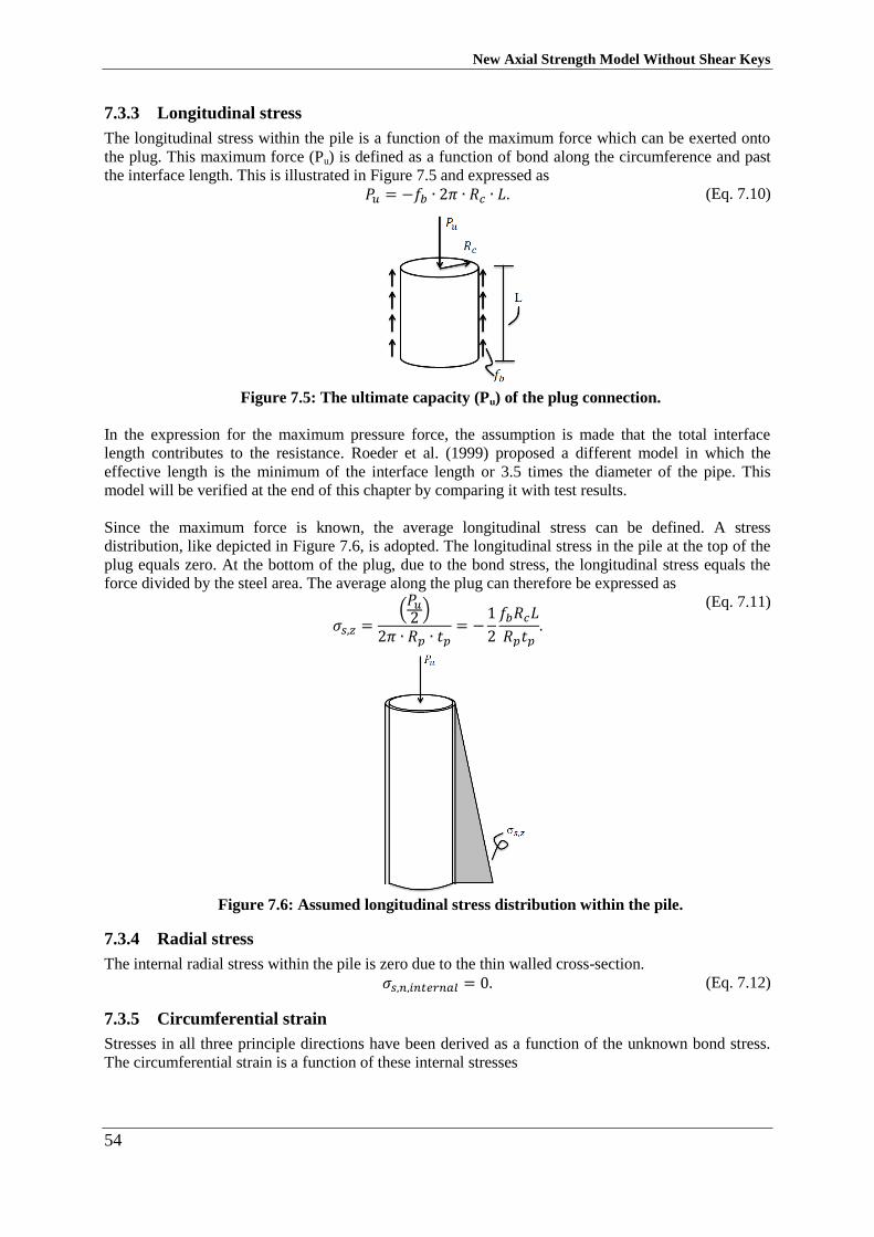
New Axial Strength Model Without Shear Keys
54
7.3.3 Longitudinal stress
The longitudinal stress within the pile is a function of the maximum force which can be exerted onto
the plug. This maximum force (Pu) is defined as a function of bond along the circumference and past
the interface length. This is illustrated in Figure 7.5 and expressed as
𝑃𝑢 = −𝑓𝑏 ∙ 2𝜋 ∙ 𝑅𝑐 ∙ 𝐿. (Eq. 7.10)
Figure 7.5: The ultimate capacity (Pu) of the plug connection.
In the expression for the maximum pressure force, the assumption is made that the total interface
length contributes to the resistance. Roeder et al. (1999) proposed a different model in which the
effective length is the minimum of the interface length or 3.5 times the diameter of the pipe. This
model will be verified at the end of this chapter by comparing it with test results.
Since the maximum force is known, the average longitudinal stress can be defined. A stress
distribution, like depicted in Figure 7.6, is adopted. The longitudinal stress in the pile at the top of the
plug equals zero. At the bottom of the plug, due to the bond stress, the longitudinal stress equals the
force divided by the steel area. The average along the plug can therefore be expressed as
𝜎𝑠,𝑧 =(𝑃𝑢2 )
2𝜋 ∙ 𝑅𝑝 ∙ 𝑡𝑝= −
1
2
𝑓𝑏𝑅𝑐𝐿
𝑅𝑝𝑡𝑝.
(Eq. 7.11)
Figure 7.6: Assumed longitudinal stress distribution within the pile.
7.3.4 Radial stress
The internal radial stress within the pile is zero due to the thin walled cross-section.
𝜎𝑠,𝑛,𝑖𝑛𝑡𝑒𝑟𝑛𝑎𝑙 = 0. (Eq. 7.12)
7.3.5 Circumferential strain
Stresses in all three principle directions have been derived as a function of the unknown bond stress.
The circumferential strain is a function of these internal stresses
New Axial Strength Model Without Shear Keys
55
휀𝑠,𝜃 =
1
𝐸𝑠(𝜎𝑠,𝜃 − 𝜈𝑠(𝜎𝑠,𝑧 + 𝜎𝑠,𝑛,𝑖𝑛𝑡𝑒𝑟𝑛𝑎𝑙)).
(Eq. 7.13)
By substituting the expressions for σs,θ, σs,z and σs,n,internal into (Eq. 7.13) results in the following
expression for the circumferential steel strain
휀𝑠,𝜃 =
1
𝐸𝑠(𝐾(𝜇𝑠 − 𝛥)𝑅𝑝
𝑡𝑝+1
2
𝜈𝑠𝑓𝑏𝑅𝑐𝐿
𝑅𝑝𝑡𝑝).
(Eq. 7.14)
Concrete stresses and strain 7.4
In contrast to the steel section, the concrete cylinder needs to be regarded as a thick walled cylinder.
This results in a different approach for defining the radial and circumferential stresses. These stresses
are defined by making use of Lame’s equations (proof is given in Appendix E)
𝜎𝑛 = 𝑎 +
𝑏
𝑅2
𝜎𝜃 = 𝑎 −𝑏
𝑅2.
(Eq. 7.15)
(Eq. 7.16)
The factors ‘a’ and ‘b’ are constants which should be solved with the boundary conditions of the
system. For the plug, the following two boundary conditions can be defined:
At the internal radius (Ri, which is actually zero), the radial stress on the plug is zero,
At the outer radius (Rc), the radial stress is equal to the exerted pressure σn (Eq. 7.6).
Solving the first boundary condition, an expression for ‘a’ can be found
0 = 𝑎 +
𝑏
𝑅𝑖2 → 𝑎 = −
𝑏
𝑅𝑖2.
(Eq. 7.17)
The second boundary condition results in an expression for ‘b’ after which ‘a’ can be solved as well.
−𝐾(𝜇𝑠 − 𝛥) = −
𝑏
𝑅𝑖2 +
𝑏
𝑅𝑐2 → 𝑏 = 𝐾(𝜇𝑠 − 𝛥)
𝑅𝑖2𝑅𝑐
2
𝑅𝑐2 − 𝑅𝑖
2 (Eq. 7.18)
and subsequently ‘a’ is equal to
𝑎 = −𝐾(𝜇𝑠 − 𝛥)
𝑅𝑐2
𝑅𝑐2 − 𝑅𝑖
2. (Eq. 7.19)
7.4.1 Circumferential and radial stress
Substituting the expression for ‘a’ and ‘b’ into (Eq. 7.15) and (Eq. 7.16), results in the expressions for
the circumferential and radial stress within the plug.
𝜎𝑐,𝜃 = −𝐾(𝜇𝑠 − 𝛥)(
𝑅𝑐2
𝑅𝑐2 − 𝑅𝑖
2 +𝑅𝑖2
𝑅𝑐2 − 𝑅𝑖
2)
𝜎𝑐,𝑛,𝑖𝑛𝑡𝑒𝑟𝑛𝑎𝑙 = −𝐾(𝜇𝑠 − 𝛥)(𝑅𝑐2
𝑅𝑐2 − 𝑅𝑖
2 −𝑅𝑖2
𝑅𝑐2 − 𝑅𝑖
2).
(Eq. 7.20)
(Eq. 7.21)
The concrete part of the connection is casted as a solid cylinder. This means that the internal radius
(Ri) is equal to zero. By doing so, the expressions for the stresses reduce to
𝜎𝑐,𝜃 = −𝐾(𝜇𝑠 − 𝛥) 𝜎𝑐,𝑛,𝑖𝑛𝑡𝑒𝑟𝑛𝑎𝑙 = −𝐾(𝜇𝑠 − 𝛥).
(Eq. 7.22)
(Eq. 7.23)
New Axial Strength Model Without Shear Keys
56
7.4.2 Longitudinal stress
The longitudinal stress can be defined as like the longitudinal stress in the pile. The opposite stress
distribution is assumed, zero stress at the bottom and Pu divided by the area at the top of the plug. This
results in
𝜎𝑐,𝑧 =(𝑃𝑢2)
𝜋𝑅𝑐2 = −
𝑓𝑏𝐿
𝑅𝑐.
(Eq. 7.24)
7.4.3 Concrete strain
Just like the steel part, the circumferential strain is a function of the three stress components.
휀𝑐,𝜃 =
1
𝐸𝑐(𝜎𝑠,𝜃 − 𝜈𝑐(𝜎𝑐,𝑧 + 𝜎𝑐,𝑛,𝑖𝑛𝑡𝑒𝑟𝑛𝑎𝑙)).
(Eq. 7.25)
By substituting (Eq. 7.22), (Eq. 7.23) and (Eq. 7.24) into the strain equation (Eq. 7.25), the following
definition for the strain is found
휀𝑐,𝜃 =
−𝐾(𝜇𝑠 − 𝛥) − 𝑣𝑐 (−𝑓𝑏𝐿𝑅𝑐
− 𝐾(𝜇𝑠 − 𝛥))
𝐸𝑐.
(Eq. 7.26)
Relative displacement between pile and plug 7.5
The relative displacement between the pile and the plug can be defined since both expressions for the
strains are known. A radial displacement (δ) is related to the circumferential strain as follows
휀𝜃 =
𝐼𝑛𝑐𝑟𝑒𝑎𝑠𝑒 𝑖𝑛 𝑐𝑖𝑟𝑐𝑢𝑚𝑓𝑒𝑟𝑒𝑛𝑐𝑒
𝐼𝑛𝑖𝑡𝑖𝑎𝑙 𝑐𝑖𝑟𝑐𝑢𝑚𝑓𝑒𝑟𝑒𝑛𝑐𝑒=2𝜋(𝑅 + 𝛿) − 2𝜋𝑅
2𝜋𝑅=𝛿
𝑅.
(Eq. 7.27)
Since the pile is considered thin walled, the radial displacement is constant along the cross-section.
The inner- and outer circumference are subjected to the same radial displacement. The strain of the
concrete varies along the axis. Both displacements at the location of the interface are therefore equal to
𝛥𝑠 = 휀𝑠,𝜃𝑅𝑝 =
(
𝐾(𝜇𝑠 − 𝛥)𝑅𝑝𝑡𝑝
+12𝜈𝑠𝑓𝑏𝑅𝑐𝐿𝑅𝑝𝑡𝑝
𝐸𝑠
)
𝑅𝑝
𝛥𝑐 = 휀𝑠,𝜃𝑅𝑐 =
(
−𝐾(𝜇𝑠 − 𝛥) − 𝑣𝑐 (
−𝑓𝑏𝐿𝑅𝑐
− 𝐾(𝜇𝑠 − 𝛥))
𝐸𝑐
)
𝑅𝑐 .
(Eq. 7.28)
(Eq. 7.29)
The relative displacement as defined in the beginning of this chapter equals
𝛥 = 𝛥𝑠 − 𝛥𝑐 . (Eq. 7.30)
Substituting (Eq. 7.28) and (Eq. 7.29) into (Eq. 7.30) gives the expression for the difference in radial
displacement
𝛥 =
(
𝐾(𝜇𝑠 − 𝛥)𝑅𝑝𝑡𝑝
+12𝜈𝑠𝑓𝑏𝑅𝑐𝐿𝑅𝑝𝑡𝑝
𝐸𝑠)
𝑅𝑝 −
(
−𝐾(𝜇𝑠 − 𝛥) − 𝑣𝑐 (
−𝑓𝑏𝐿𝑅𝑐
− 𝐾(𝜇𝑠 − 𝛥))
𝐸𝑐
)
𝑅𝑐.
(Eq. 7.31)
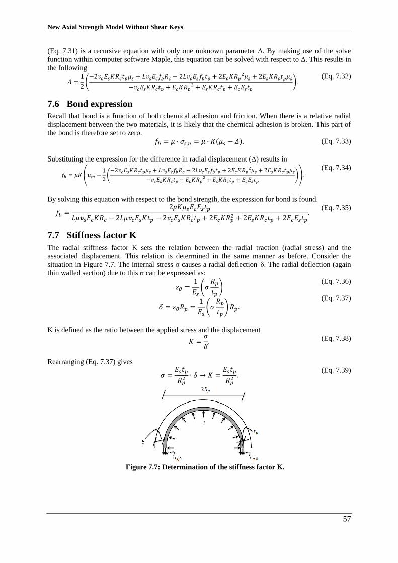
New Axial Strength Model Without Shear Keys
57
(Eq. 7.31) is a recursive equation with only one unknown parameter Δ. By making use of the solve
function within computer software Maple, this equation can be solved with respect to Δ. This results in
the following
𝛥 =
1
2(−2𝑣𝑐𝐸𝑠𝐾𝑅𝑐𝑡𝑝𝜇𝑠 + 𝐿𝑣𝑠𝐸𝑐𝑓𝑏𝑅𝑐 − 2𝐿𝑣𝑐𝐸𝑠𝑓𝑏𝑡𝑝 + 2𝐸𝑐𝐾𝑅𝑝
2𝜇𝑠 + 2𝐸𝑠𝐾𝑅𝑐𝑡𝑝𝜇𝑠
−𝑣𝑐𝐸𝑠𝐾𝑅𝑐𝑡𝑝 + 𝐸𝑐𝐾𝑅𝑝2 + 𝐸𝑠𝐾𝑅𝑐𝑡𝑝 + 𝐸𝑐𝐸𝑠𝑡𝑝
). (Eq. 7.32)
Bond expression 7.6
Recall that bond is a function of both chemical adhesion and friction. When there is a relative radial
displacement between the two materials, it is likely that the chemical adhesion is broken. This part of
the bond is therefore set to zero.
𝑓𝑏 = 𝜇 ∙ 𝜎𝑠,𝑛 = 𝜇 ∙ 𝐾(𝜇𝑠 − 𝛥). (Eq. 7.33)
Substituting the expression for the difference in radial displacement (Δ) results in
𝑓𝑏 = 𝜇𝐾(𝑢𝑚 −
1
2(−2𝑣𝑐𝐸𝑠𝐾𝑅𝑐𝑡𝑝𝜇𝑠 + 𝐿𝑣𝑠𝐸𝑐𝑓𝑏𝑅𝑐 − 2𝐿𝑣𝑐𝐸𝑠𝑓𝑏𝑡𝑝 + 2𝐸𝑐𝐾𝑅𝑝
2𝜇𝑠 + 2𝐸𝑠𝐾𝑅𝑐𝑡𝑝𝜇𝑠
−𝑣𝑐𝐸𝑠𝐾𝑅𝑐𝑡𝑝 + 𝐸𝑐𝐾𝑅𝑝2 + 𝐸𝑠𝐾𝑅𝑐𝑡𝑝 + 𝐸𝑐𝐸𝑠𝑡𝑝
)). (Eq. 7.34)
By solving this equation with respect to the bond strength, the expression for bond is found.
𝑓𝑏 =
2𝜇𝐾𝜇𝑠𝐸𝑐𝐸𝑠𝑡𝑝
𝐿𝜇𝑣𝑠𝐸𝑐𝐾𝑅𝑐 − 2𝐿𝜇𝑣𝑐𝐸𝑠𝐾𝑡𝑝 − 2𝑣𝑐𝐸𝑠𝐾𝑅𝑐𝑡𝑝 + 2𝐸𝑐𝐾𝑅𝑝2 + 2𝐸𝑠𝐾𝑅𝑐𝑡𝑝 + 2𝐸𝑐𝐸𝑠𝑡𝑝
. (Eq. 7.35)
Stiffness factor K 7.7
The radial stiffness factor K sets the relation between the radial traction (radial stress) and the
associated displacement. This relation is determined in the same manner as before. Consider the
situation in Figure 7.7. The internal stress σ causes a radial deflection δ. The radial deflection (again
thin walled section) due to this σ can be expressed as:
휀𝜃 =
1
𝐸𝑠(𝜎𝑅𝑝𝑡𝑝)
𝛿 = 휀𝜃𝑅𝑝 =1
𝐸𝑠(𝜎𝑅𝑝𝑡𝑝)𝑅𝑝.
(Eq. 7.36)
(Eq. 7.37)
K is defined as the ratio between the applied stress and the displacement
𝐾 =𝜎
𝛿. (Eq. 7.38)
Rearranging (Eq. 7.37) gives
𝜎 =
𝐸𝑠𝑡𝑝
𝑅𝑝2 ∙ 𝛿 → 𝐾 =
𝐸𝑠𝑡𝑝
𝑅𝑝2 .
(Eq. 7.39)
Figure 7.7: Determination of the stiffness factor K.
New Axial Strength Model Without Shear Keys
58
7.7.1 Comparing stiffness factors
Comparing the derived factor with the one from Billington et al. (1978), shows substantial differences.
The one from Billington (Eq. 6.6) is related to the radius of the pile whilst in the derived formulation it
is related to the radius squared. This means that the formulation is way more sensitive to scale effects,
which is in line with test results from chapter 6. A comparison of the units gives
𝐾𝑎𝑛𝑎𝑙𝑦𝑡𝑖𝑐𝑎𝑙𝑙𝑦 =
[𝑁]
[𝑚𝑚]2[𝑚𝑚]
[𝑚𝑚]2= [
𝑁
𝑚𝑚3]
𝐾𝐵𝑖𝑙𝑙𝑖𝑛𝑔𝑡𝑜𝑛 =[𝑁]
[𝑚𝑚]2[𝑚𝑚]
[𝑚𝑚]= [
𝑁
𝑚𝑚2].
(Eq. 7.40)
(Eq. 7.41)
When both formulations are checked, it seems that the formula, formulated by Billington et al. (1978)
to which current design formulations are based, is incorrect. In the denoted paper, the stiffness factor
is introduced as an approximation rather than an equality. This might be the reason that current
formulations diverge with large pile diameters.
Bond formulation 7.8
The expression for the bond strength from section 7.6 can be shortened. The following properties are
adopted:
The friction coefficient between steel and concrete (μ) is examined by Rabbat et al. (1985).
The purpose of their research was to examine the friction coefficient in containment vessels by
testing. For a dry interface (meaning that the concrete has hardened), a value for μ of 0.57 is
found. ECS (2011c) prescribes a value of 0.5 for steel without paint. This latter value is
considered safe and will be used,
The surface roughness of the steel (μs) can be taken as 0.05mm for steel sections (ECS
(2005)),
The Poisson ratio for steel is 0.3 and for concrete 0.2.
Applying the previous values for the friction, roughness and Poisson ratios together with the derived
stiffness factor K (Eq. 7.39), the bond expression reduces to
𝑓𝑏,𝑝𝑢𝑠ℎ−𝑜𝑢𝑡 =
𝐸𝑠𝑡𝑝
𝑅𝑐(3𝐿 + 32𝑚𝑡𝑝) − 4𝐿𝑚𝑡𝑝 + 80𝑅𝑝2.
(Eq. 7.42)
In which m is defined as the modular ratio (Es/Ec). Note that this is the expression for the push-out
mechanism of the plug. When the complete derivation is deduced again for pull-out, the following
formulation is found
𝑓𝑏,𝑝𝑢𝑙𝑙−𝑜𝑢𝑡 =
𝐸𝑠𝑡𝑝
𝑅𝑐(3𝐿 − 32𝑚𝑡𝑝) − 4𝐿𝑚𝑡𝑝 − 80𝑅𝑝2.
(Eq. 7.43)
Final bond formulation including shrinkage 7.9
Shrinkage is denoted as one of the most influencing factors on the bond capacity and therefore it
should be incorporated in the model. In the equation for the concrete strain (Eq. 7.26), an additional
shrinkage term (εshrinkage) is included. This equation changes to
휀𝑐,𝑛 =1
𝐸𝑐(−𝐾(𝜇𝑠 − 𝛥) − 𝑣𝑐 (
−𝑓𝑏𝐿
𝑅𝑐− 𝐾(𝜇𝑠 − 𝛥))) − 휀𝑠ℎ𝑟𝑖𝑛𝑘𝑎𝑔𝑒 .
(Eq. 7.44)
By rerunning the analysis and resolving the equations, the bond formulations (including shrinkage) are
found
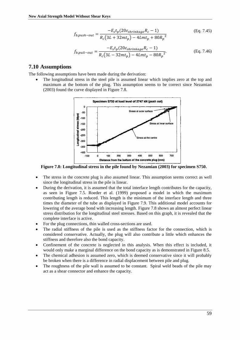
New Axial Strength Model Without Shear Keys
59
𝑓𝑏,𝑝𝑢𝑠ℎ−𝑜𝑢𝑡 =
−𝐸𝑠𝑡𝑝(20휀𝑠ℎ𝑟𝑖𝑛𝑘𝑎𝑔𝑒𝑅𝑐 − 1)
𝑅𝑐(3𝐿 + 32𝑚𝑡𝑝) − 4𝐿𝑚𝑡𝑝 + 80𝑅𝑝2
𝑓𝑏,𝑝𝑢𝑙𝑙−𝑜𝑢𝑡 =−𝐸𝑠𝑡𝑝(20휀𝑠ℎ𝑟𝑖𝑛𝑘𝑎𝑔𝑒𝑅𝑐 − 1)
𝑅𝑐(3𝐿 − 32𝑚𝑡𝑝) − 4𝐿𝑚𝑡𝑝 − 80𝑅𝑝2.
(Eq. 7.45)
(Eq. 7.46)
Assumptions 7.10
The following assumptions have been made during the derivation:
The longitudinal stress in the steel pile is assumed linear which implies zero at the top and
maximum at the bottom of the plug. This assumption seems to be correct since Nezamian
(2003) found the curve displayed in Figure 7.8.
Figure 7.8: Longitudinal stress in the pile found by Nezamian (2003) for specimen S750.
The stress in the concrete plug is also assumed linear. This assumption seems correct as well
since the longitudinal stress in the pile is linear.
During the derivation, it is assumed that the total interface length contributes for the capacity,
as seen in Figure 7.5. Roeder et al. (1999) proposed a model in which the maximum
contributing length is reduced. This length is the minimum of the interface length and three
times the diameter of the tube as displayed in Figure 7.9. This additional model accounts for
lowering of the average bond with increasing length. Figure 7.8 shows an almost perfect linear
stress distribution for the longitudinal steel stresses. Based on this graph, it is revealed that the
complete interface is active.
For the plug connections, thin walled cross-sections are used.
The radial stiffness of the pile is used as the stiffness factor for the connection, which is
considered conservative. Actually, the plug will also contribute a little which enhances the
stiffness and therefore also the bond capacity.
Confinement of the concrete is neglected in this analysis. When this effect is included, it
would only make a marginal difference on the bond capacity as is demonstrated in Figure 8.5.
The chemical adhesion is assumed zero, which is deemed conservative since it will probably
be broken when there is a difference in radial displacement between pile and plug.
The roughness of the pile wall is assumed to be constant. Spiral weld beads of the pile may
act as a shear connector and enhance the capacity.
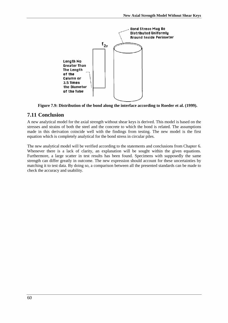
New Axial Strength Model Without Shear Keys
60
Figure 7.9: Distribution of the bond along the interface according to Roeder et al. (1999).
Conclusion 7.11
A new analytical model for the axial strength without shear keys is derived. This model is based on the
stresses and strains of both the steel and the concrete to which the bond is related. The assumptions
made in this derivation coincide well with the findings from testing. The new model is the first
equation which is completely analytical for the bond stress in circular piles.
The new analytical model will be verified according to the statements and conclusions from Chapter 6.
Whenever there is a lack of clarity, an explanation will be sought within the given equations.
Furthermore, a large scatter in test results has been found. Specimens with supposedly the same
strength can differ greatly in outcome. The new expression should account for these uncertainties by
matching it to test data. By doing so, a comparison between all the presented standards can be made to
check the accuracy and usability.
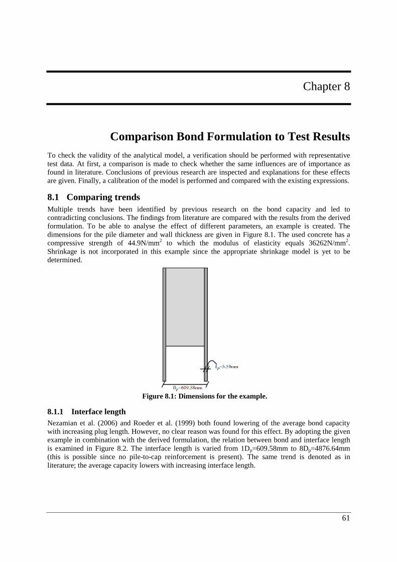
61
Chapter 8
8. Comparison Bond Formulation to Test Results
To check the validity of the analytical model, a verification should be performed with representative
test data. At first, a comparison is made to check whether the same influences are of importance as
found in literature. Conclusions of previous research are inspected and explanations for these effects
are given. Finally, a calibration of the model is performed and compared with the existing expressions.
Comparing trends 8.1
Multiple trends have been identified by previous research on the bond capacity and led to
contradicting conclusions. The findings from literature are compared with the results from the derived
formulation. To be able to analyse the effect of different parameters, an example is created. The
dimensions for the pile diameter and wall thickness are given in Figure 8.1. The used concrete has a
compressive strength of 44.9N/mm2 to which the modulus of elasticity equals 36262N/mm
2.
Shrinkage is not incorporated in this example since the appropriate shrinkage model is yet to be
determined.
Figure 8.1: Dimensions for the example.
8.1.1 Interface length
Nezamian et al. (2006) and Roeder et al. (1999) both found lowering of the average bond capacity
with increasing plug length. However, no clear reason was found for this effect. By adopting the given
example in combination with the derived formulation, the relation between bond and interface length
is examined in Figure 8.2. The interface length is varied from 1Dp=609.58mm to 8Dp=4876.64mm
(this is possible since no pile-to-cap reinforcement is present). The same trend is denoted as in
literature; the average capacity lowers with increasing interface length.
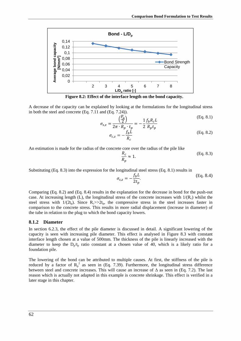
Comparison Bond Formulation to Test Results
62
Figure 8.2: Effect of the interface length on the bond capacity.
A decrease of the capacity can be explained by looking at the formulations for the longitudinal stress
in both the steel and concrete (Eq. 7.11 and (Eq. 7.24)).
𝜎𝑠,𝑧 =(𝑃𝑢2)
2𝜋 ∙ 𝑅𝑝 ∙ 𝑡𝑝= −
1
2
𝑓𝑏𝑅𝑐𝐿
𝑅𝑝𝑡𝑝
𝜎𝑐,𝑧 = −𝑓𝑏𝐿
𝑅𝑐
(Eq. 8.1)
(Eq. 8.2)
An estimation is made for the radius of the concrete core over the radius of the pile like
𝑅𝑐𝑅𝑝≈ 1.
(Eq. 8.3)
Substituting (Eq. 8.3) into the expression for the longitudinal steel stress (Eq. 8.1) results in
𝜎𝑠,𝑧 = −
𝑓𝑏𝐿
2𝑡𝑝.
(Eq. 8.4)
Comparing (Eq. 8.2) and (Eq. 8.4) results in the explanation for the decrease in bond for the push-out
case. At increasing length (L), the longitudinal stress of the concrete increases with 1/(Rc) whilst the
steel stress with 1/(2tp). Since Rc>>2tp, the compressive stress in the steel increases faster in
comparison to the concrete stress. This results in more radial displacement (increase in diameter) of
the tube in relation to the plug to which the bond capacity lowers.
8.1.2 Diameter
In section 6.2.3, the effect of the pile diameter is discussed in detail. A significant lowering of the
capacity is seen with increasing pile diameter. This effect is analysed in Figure 8.3 with constant
interface length chosen at a value of 500mm. The thickness of the pile is linearly increased with the
diameter to keep the Dp/tp ratio constant at a chosen value of 40, which is a likely ratio for a
foundation pile.
The lowering of the bond can be attributed to multiple causes. At first, the stiffness of the pile is
reduced by a factor of Rp2 as seen in (Eq. 7.39). Furthermore, the longitudinal stress difference
between steel and concrete increases. This will cause an increase of Δ as seen in (Eq. 7.2). The last
reason which is actually not adapted in this example is concrete shrinkage. This effect is verified in a
later stage in this chapter.
0
0,02
0,04
0,06
0,08
0,1
0,12
0,14
2 3 4 5 6 7 8
Ave
rag
e b
on
d c
ap
ac
ity
[N/m
m2]
L/Dp ratio [-]
Bond - L/Dp
Bond StrengthCapacity
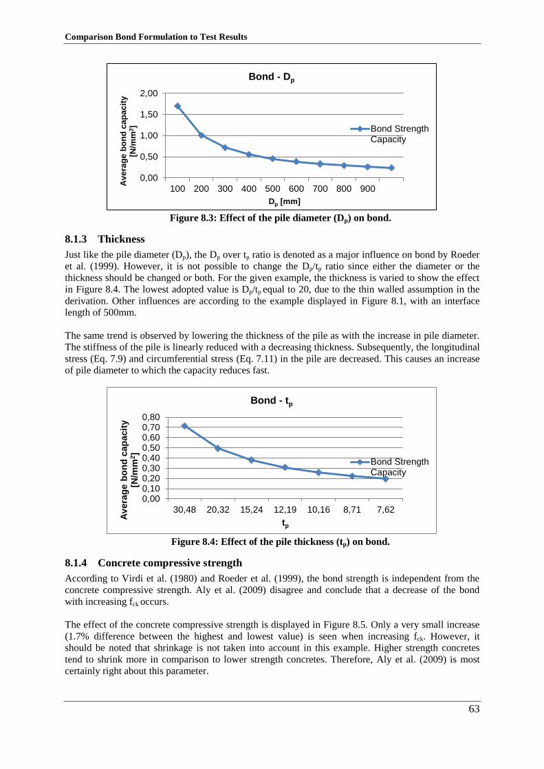
Comparison Bond Formulation to Test Results
63
Figure 8.3: Effect of the pile diameter (Dp) on bond.
8.1.3 Thickness
Just like the pile diameter (Dp), the Dp over tp ratio is denoted as a major influence on bond by Roeder
et al. (1999). However, it is not possible to change the Dp/tp ratio since either the diameter or the
thickness should be changed or both. For the given example, the thickness is varied to show the effect
in Figure 8.4. The lowest adopted value is Dp/tp equal to 20, due to the thin walled assumption in the
derivation. Other influences are according to the example displayed in Figure 8.1, with an interface
length of 500mm.
The same trend is observed by lowering the thickness of the pile as with the increase in pile diameter.
The stiffness of the pile is linearly reduced with a decreasing thickness. Subsequently, the longitudinal
stress (Eq. 7.9) and circumferential stress (Eq. 7.11) in the pile are decreased. This causes an increase
of pile diameter to which the capacity reduces fast.
Figure 8.4: Effect of the pile thickness (tp) on bond.
8.1.4 Concrete compressive strength
According to Virdi et al. (1980) and Roeder et al. (1999), the bond strength is independent from the
concrete compressive strength. Aly et al. (2009) disagree and conclude that a decrease of the bond
with increasing fck occurs.
The effect of the concrete compressive strength is displayed in Figure 8.5. Only a very small increase
(1.7% difference between the highest and lowest value) is seen when increasing fck. However, it
should be noted that shrinkage is not taken into account in this example. Higher strength concretes
tend to shrink more in comparison to lower strength concretes. Therefore, Aly et al. (2009) is most
certainly right about this parameter.
0,00
0,50
1,00
1,50
2,00
100 200 300 400 500 600 700 800 900
Ave
rag
e b
on
d c
ap
ac
ity
[N/m
m2]
Dp [mm]
Bond - Dp
Bond StrengthCapacity
0,000,100,200,300,400,500,600,700,80
30,48 20,32 15,24 12,19 10,16 8,71 7,62
Av
era
ge b
on
d c
ap
acit
y
[N/m
m2]
tp
Bond - tp
Bond StrengthCapacity
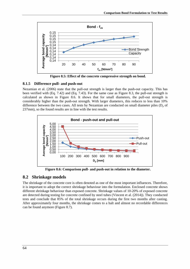
Comparison Bond Formulation to Test Results
64
Figure 8.5: Effect of the concrete compressive strength on bond.
8.1.5 Difference pull- and push-out
Nezamian et al. (2006) state that the pull-out strength is larger than the push-out capacity. This has
been verified with (Eq. 7.42) and (Eq. 7.43). For the same case as Figure 8.3, the pull-out strength is
calculated as shown in Figure 8.6. It shows that for small diameters, the pull-out strength is
considerably higher than the push-out strength. With larger diameters, this reduces to less than 10%
difference between the two cases. All tests by Nezamian are conducted on small diameter piles (Dp of
237mm), so the found results are in line with the test results.
Figure 8.6: Comparison pull- and push-out in relation to the diameter.
Shrinkage models 8.2
The shrinkage of the concrete core is often denoted as one of the most important influences. Therefore,
it is important to adopt the correct shrinkage behaviour into the formulation. Enclosed concrete shows
different shrinkage behaviour than exposed concrete. Shrinkage values of 10-20% of exposed concrete
are detected during testing for concrete confined by steel tubes (Vincent et al. (2014)). They conducted
tests and conclude that 85% of the total shrinkage occurs during the first two months after casting.
After approximately four months, the shrinkage comes to a halt and almost no recordable differences
can be found anymore (Figure 8.7).
0,140,140,140,140,140,140,150,150,150,15
20 30 40 50 60 70 80 90
Av
era
ge b
on
d c
ap
acit
y
[N/m
m2]
fck [N/mm2]
Bond - fck
Bond StrengthCapacity
0,000,501,001,502,002,503,003,504,004,505,00
100 200 300 400 500 600 700 800 900Ave
rag
e b
on
d c
ap
ac
ity
[N/m
m2]
Dp [mm]
Bond - push-out and pull-out
Push-out
Pull-out
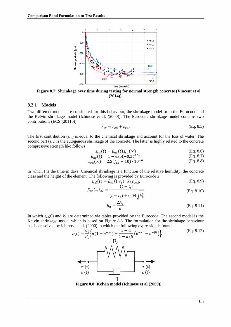
Comparison Bond Formulation to Test Results
65
Figure 8.7: Shrinkage over time during testing for normal strength concrete (Vincent et al.
(2014)).
8.2.1 Models
Two different models are considered for this behaviour, the shrinkage model from the Eurocode and
the Kelvin shrinkage model (Ichinose et al. (2000)). The Eurocode shrinkage model contains two
contributions (ECS (2011b))
휀𝑐𝑠 = 휀𝑐𝑑 + 휀𝑐𝑎 . (Eq. 8.5)
The first contribution (εcd) is equal to the chemical shrinkage and account for the loss of water. The
second part (εca) is the autogenous shrinkage of the concrete. The latter is highly related to the concrete
compressive strength like follows
휀𝑐𝑎(𝑡) = 𝛽𝑎𝑠(𝑡)휀𝑐𝑎(∞) 𝛽𝑎𝑠(𝑡) = 1 − exp(−0.2𝑡
0.5) 휀𝑐𝑎(∞) = 2.5(𝑓𝑐𝑘 − 10) ∙ 10
−6
(Eq. 8.6)
(Eq. 8.7)
(Eq. 8.8)
in which t is the time in days. Chemical shrinkage is a function of the relative humidity, the concrete
class and the height of the element. The following is provided by Eurocode 2
휀𝑐𝑑(𝑡) = 𝛽𝑑𝑠(𝑡, 𝑡𝑠) ∙ 𝑘ℎ휀𝑐𝑑,0
𝛽𝑑𝑠(𝑡, 𝑡𝑠) =(𝑡 − 𝑡𝑠)
(𝑡 − 𝑡𝑠) + 0.04√ℎ03
ℎ0 =2𝐴𝑐𝑢.
(Eq. 8.9)
(Eq. 8.10)
(Eq. 8.11)
In which εcd(0) and kh are determined via tables provided by the Eurocode. The second model is the
Kelvin shrinkage model which is based on Figure 8.8. The formulation for the shrinkage behaviour
has been solved by Ichinose et al. (2000) to which the following expression is found
휀(𝑡) =
𝜎0𝐸𝑐{𝛼(1 − 𝑒−𝜅𝑡) +
1 − 𝛼
1 − 𝜅/𝛽(𝑒−𝜅𝑡 − 𝑒−𝛽𝑡)}.
(Eq. 8.12)
Figure 8.8: Kelvin model (Ichinose et al.(2000)).
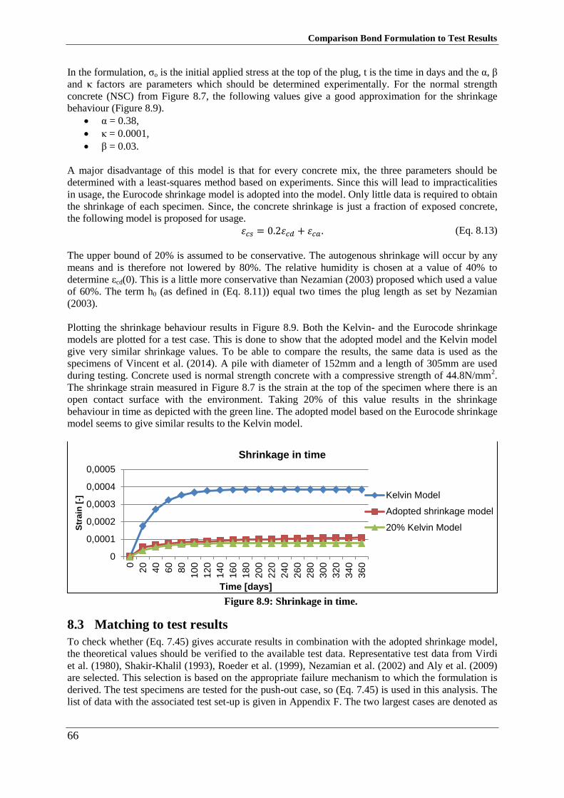
Comparison Bond Formulation to Test Results
66
In the formulation, σo is the initial applied stress at the top of the plug, t is the time in days and the α, β
and κ factors are parameters which should be determined experimentally. For the normal strength
concrete (NSC) from Figure 8.7, the following values give a good approximation for the shrinkage
behaviour (Figure 8.9).
α = 0.38,
κ = 0.0001,
β = 0.03.
A major disadvantage of this model is that for every concrete mix, the three parameters should be
determined with a least-squares method based on experiments. Since this will lead to impracticalities
in usage, the Eurocode shrinkage model is adopted into the model. Only little data is required to obtain
the shrinkage of each specimen. Since, the concrete shrinkage is just a fraction of exposed concrete,
the following model is proposed for usage.
휀𝑐𝑠 = 0.2휀𝑐𝑑 + 휀𝑐𝑎 . (Eq. 8.13)
The upper bound of 20% is assumed to be conservative. The autogenous shrinkage will occur by any
means and is therefore not lowered by 80%. The relative humidity is chosen at a value of 40% to
determine εcd(0). This is a little more conservative than Nezamian (2003) proposed which used a value
of 60%. The term h0 (as defined in (Eq. 8.11)) equal two times the plug length as set by Nezamian
(2003).
Plotting the shrinkage behaviour results in Figure 8.9. Both the Kelvin- and the Eurocode shrinkage
models are plotted for a test case. This is done to show that the adopted model and the Kelvin model
give very similar shrinkage values. To be able to compare the results, the same data is used as the
specimens of Vincent et al. (2014). A pile with diameter of 152mm and a length of 305mm are used
during testing. Concrete used is normal strength concrete with a compressive strength of 44.8N/mm2.
The shrinkage strain measured in Figure 8.7 is the strain at the top of the specimen where there is an
open contact surface with the environment. Taking 20% of this value results in the shrinkage
behaviour in time as depicted with the green line. The adopted model based on the Eurocode shrinkage
model seems to give similar results to the Kelvin model.
Figure 8.9: Shrinkage in time.
Matching to test results 8.3
To check whether (Eq. 7.45) gives accurate results in combination with the adopted shrinkage model,
the theoretical values should be verified to the available test data. Representative test data from Virdi
et al. (1980), Shakir-Khalil (1993), Roeder et al. (1999), Nezamian et al. (2002) and Aly et al. (2009)
are selected. This selection is based on the appropriate failure mechanism to which the formulation is
derived. The test specimens are tested for the push-out case, so (Eq. 7.45) is used in this analysis. The
list of data with the associated test set-up is given in Appendix F. The two largest cases are denoted as
0
0,0001
0,0002
0,0003
0,0004
0,0005
0
20
40
60
80
10
0
12
0
14
0
16
0
18
0
20
0
22
0
24
0
26
0
28
0
30
0
32
0
34
0
36
0
Str
ain
[-]
Time [days]
Shrinkage in time
Kelvin Model
Adopted shrinkage model
20% Kelvin Model
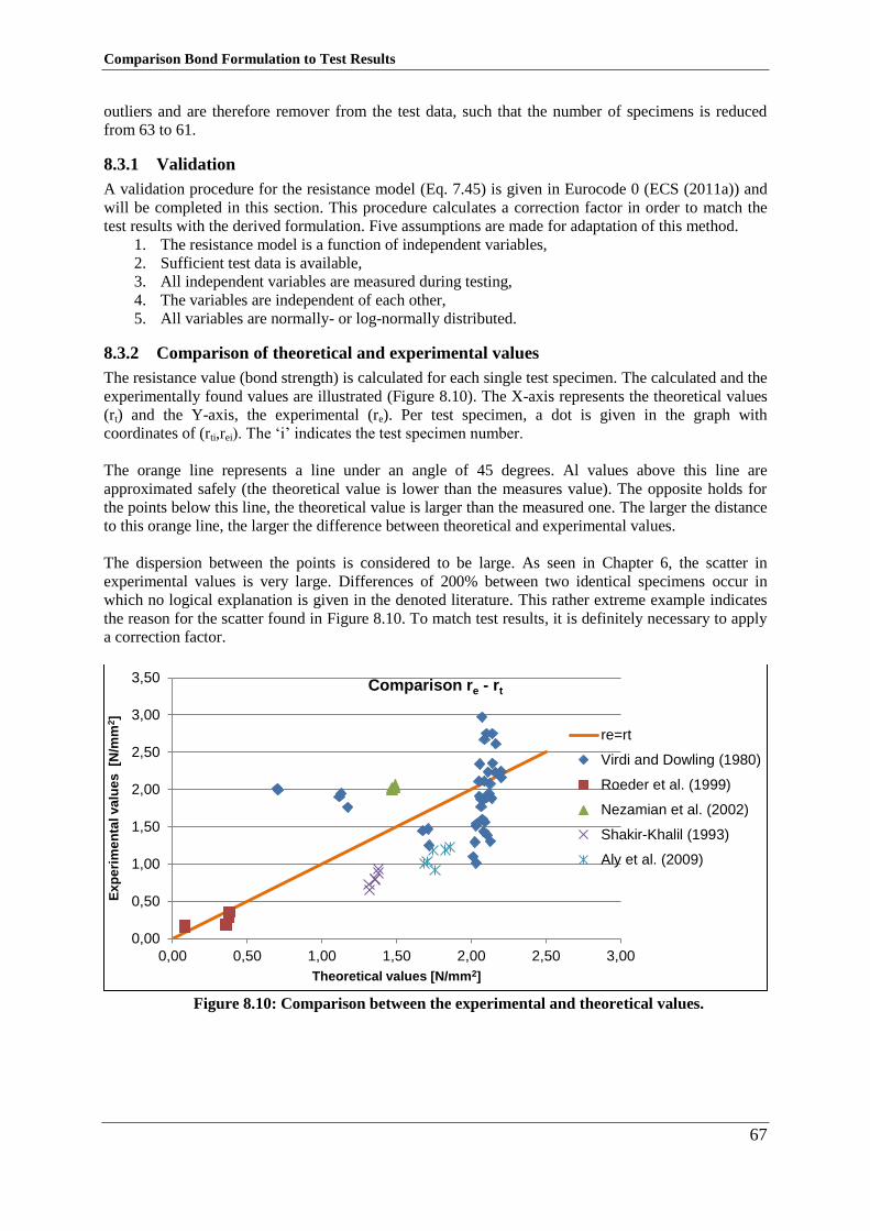
Comparison Bond Formulation to Test Results
67
outliers and are therefore remover from the test data, such that the number of specimens is reduced
from 63 to 61.
8.3.1 Validation
A validation procedure for the resistance model (Eq. 7.45) is given in Eurocode 0 (ECS (2011a)) and
will be completed in this section. This procedure calculates a correction factor in order to match the
test results with the derived formulation. Five assumptions are made for adaptation of this method.
1. The resistance model is a function of independent variables,
2. Sufficient test data is available,
3. All independent variables are measured during testing,
4. The variables are independent of each other,
5. All variables are normally- or log-normally distributed.
8.3.2 Comparison of theoretical and experimental values
The resistance value (bond strength) is calculated for each single test specimen. The calculated and the
experimentally found values are illustrated (Figure 8.10). The X-axis represents the theoretical values
(rt) and the Y-axis, the experimental (re). Per test specimen, a dot is given in the graph with
coordinates of (rti,rei). The ‘i’ indicates the test specimen number.
The orange line represents a line under an angle of 45 degrees. Al values above this line are
approximated safely (the theoretical value is lower than the measures value). The opposite holds for
the points below this line, the theoretical value is larger than the measured one. The larger the distance
to this orange line, the larger the difference between theoretical and experimental values.
The dispersion between the points is considered to be large. As seen in Chapter 6, the scatter in
experimental values is very large. Differences of 200% between two identical specimens occur in
which no logical explanation is given in the denoted literature. This rather extreme example indicates
the reason for the scatter found in Figure 8.10. To match test results, it is definitely necessary to apply
a correction factor.
Figure 8.10: Comparison between the experimental and theoretical values.
0,00
0,50
1,00
1,50
2,00
2,50
3,00
3,50
0,00 0,50 1,00 1,50 2,00 2,50 3,00
Ex
pe
rim
en
tal va
lue
s [N
/mm
2]
Theoretical values [N/mm2]
Comparison re - rt
re=rt
Virdi and Dowling (1980)
Roeder et al. (1999)
Nezamian et al. (2002)
Shakir-Khalil (1993)
Aly et al. (2009)
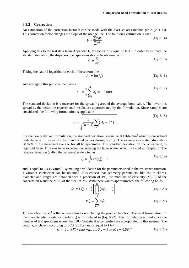
Comparison Bond Formulation to Test Results
68
8.3.3 Correction
An estimation of the correction factor b can be made with the least squares method (ECS (2011a)).
This correction factor changes the slope of the orange line. The following estimation is used
𝑏 =
∑𝑟𝑒𝑟𝑡∑𝑟𝑡
2 . (Eq. 8.14)
Applying this to the test data from Appendix F, the factor b is equal to 0.90. In order to estimate the
standard deviation, the dispersion per specimen should be obtained with
𝛿𝑖 =𝑟𝑒𝑖𝑏𝑟𝑡𝑖
. (Eq. 8.15)
Taking the natural logarithm of each of these term like
𝛥𝑖 = ln(𝛿𝑖) (Eq. 8.16)
and averaging this per specimen gives
𝛥− =
1
𝑛∑𝛥𝑖
𝑛
𝑖=1
= −0.009. (Eq. 8.17)
The standard deviation is a measure for the spreading around the average bond value. The lower this
spread is, the better the experimental results are approximated by the formulation. Since samples are
considered, the following formulation is applicable
𝑠𝛥 = √
1
(𝑛 − 1)∑( 𝛥𝑖 − 𝛥
−)2𝑛
𝑖=1
.
(Eq. 8.18)
For the newly derived formulation, the standard deviation is equal to 0.416N/mm2 which is considered
quite large with respect to the found bond values during testing. The average calculated strength is
98.92% of the measured average for all 61 specimens. The standard deviation on the other hand, is
regarded large. This was to be expected considering the huge scatter which is found in Chapter 6. The
relative deviation (called the variance) is denoted as
𝑉𝛿 = √exp(𝑠𝛥
2) − 1 (Eq. 8.19)
and is equal to 0.435N/mm2. By making a validation for the parameters used in the resistance function,
a variance coefficient can be obtained. It is chosen that geometry parameters, like the thickness,
diameter and length are obtained with a precision of 1%, the modulus of elasticity (MOE) of the
concrete 20% and the MOE of the steel of 7%. With these values approximated, the following holds
𝑉𝑟2 = (𝑉𝛿
2 + 1) [∏(𝑣𝑋𝑖2 + 1)
𝑛
𝑖=1
] − 1
𝑉𝑟𝑡2 =∑𝑉𝑋𝑖
2
𝑗
𝑖=1
.
(Eq. 8.20)
(Eq. 8.21)
This function for Vr2 is the variance function including the product function. The final formulation for
the characteristic resistance model (rk) is formulated in (Eq. 8.22). This formulation is used since the
number of test specimens is less than 100. Statistical uncertainties are incorporated in this manner. The
factor kn is chosen according to ECS (2011a) and is equal to 1.64.
𝑟𝑘 = 𝑏𝑔𝑟𝑡(𝑋) ∙ exp(−𝑘∞𝛼𝑟𝑡𝑄𝑟𝑡 − 𝑘𝑛𝛼𝛿𝑄𝛿 − 0.5𝑄2) (Eq. 8.22)
Comparison Bond Formulation to Test Results
69
In which:
𝑄𝑟𝑡 = √𝑙𝑛(𝑉𝑟𝑡
2 + 1) = 0.058 (Eq. 8.23)
𝑄𝛿 = √𝑙𝑛(𝑉𝛿
2 + 1) = 0.417 (Eq. 8.24)
𝑄 = √𝑙𝑛(𝑉
𝑟2 + 1) = 0.421
(Eq. 8.25)
𝛼𝑟𝑡 =
𝑄𝑟𝑡𝑄= 0.139
(Eq. 8.26)
𝛼𝛿 =
𝑄𝛿𝑄= 0.990
(Eq. 8.27)
With k∞ equal to 1.64, the factor to calibrate the derived formulation to the test results is equal to 0.40.
The resistance function therefore changes to
𝑓𝑏,𝑝𝑢𝑠ℎ−𝑜𝑢𝑡 = 0.40 ∙
−𝐸𝑠𝑡𝑝(20휀𝑠ℎ𝑟𝑖𝑛𝑘𝑎𝑔𝑒𝑅𝑐 − 1)
𝑅𝑐(3𝐿 + 32𝑚𝑡𝑝) − 4𝐿𝑚𝑡𝑝 + 80𝑅𝑝2.
(Eq. 8.28)
8.3.4 Comparison with correction factor
The effect of this correction factor can be seen in the re-rt graph. When the graph of Figure 8.10 is
redrawn including the correction factor, Figure 8.11 is obtained. All data points are now above the
orange line which indicates that the calculated numbers are below the measured values. The average
calculated bond (including correction factor) for the 61 specimens is 0.67N/mm2.
Figure 8.11: Comparison between the experimental and theoretical values with the
correction factor.
Comparison with other expressions 8.4
To put the obtained numbers from the previous section into perspective, the same analysis is
performed using the bond formulation of Roeder et al. (1999)
𝑓𝑏 = 2.109 − 0.026(𝐷𝑝 𝑡𝑝⁄ ). (Eq. 8.29)
The expression is obtained with a regression analysis based on experimental data, partly similar to the
data used in this report. The bond expression is derived in order that only 2.5% of the measurements
exceed the predicted strength.
0,00
0,50
1,00
1,50
2,00
2,50
3,00
3,50
0,00 0,50 1,00 1,50 2,00 2,50 3,00
Ex
pe
rim
en
tal va
lue
s [
N/m
m2]
Theoretical values [N/mm2]
Comparison re - rt with correction
re=rt
Virdi and Dowling (1980)
Roeder et al. (1999)
Nezamian et al. (2002)
Shakir-Khalil (1993)
Aly et al. (2009)
Comparison Bond Formulation to Test Results
70
The sample standard deviation for the formulation from (Eq. 8.29) is 0.46N/mm2 which is 18.5%
larger in comparison to the standard deviation of the derived formula. The final correction factor is
0.46, which is 15% higher than before. This is attributed to the conservative nature of the regression
analysis. The factor b (Eq. 8.14) is relative large to which the correction factor is relative high
regarding the large standard deviation. When the correction factor of 0.46 is applied and verified
against the test data, an average of 0.64N/mm2 is found. This is 5% lower in comparison to the new
formula. A remarkable detail is that of all data, the own test results by Roeder et al. (1999) are
approximated the worst. Even with the applied correction factor, the measured data is still lower than
the calculated ones.
The results of this analysis for all design expressions (without design factors) are given in Table 8.1.
The expressions are used in combination with the proposed stiffness factor by Nezamian et al. (2003).
(Eq. 7.39) has also been tried as stiffness factor but performed much worse. The derived formula (DF)
has the lowest standard deviation (SD) and when applying the correction factor, it has the largest
average for all 61 specimens within a safe margin. This implies that the most accurate and the highest
bond stresses are obtained for the derived formulation within a safe margin. The most right column
indicates the percentage of the average in relation to the derived formulation. The API, the British
Standard (BS) and the Eurocode (EC) which prescribe constant bond values, all result in similar
results. The average to be used according to these standards is 0.38N/mm2. Based on the selection of
test specimens used in this report, the British Standard seems to use the most appropriate value of
0.4N/mm2. The Eurocode value of 0.55N/mm
2 is, based on this analysis, regarded not safe. This value
will hold for small diameter pipe piles. It must be noted that when more test data on large pile is
available, the average of all three codes will drop drastically.
Table 8.1: Comparison of all design expressions.
Formulation SD
[N/mm2]
Correction factor Average
[N/mm2]
Percentage of av.
[%]
DF 0.42 0.40 0.67 100%
Roeder (1999) 0.46 0.46 0.64 95%
Norsok (2012) 0.47 0.16 0.61 91%
EC (2011) 0.72 0.69 0.38 57%
BS (1999) 0.73 0.95 0.38 57%
API (2003) 0.75 1.53 0.38 57%
OT (2002) 0.78 0.05 0.29 43%
8.4.1 Design factors
The design factors (including safety factors, material factors etc.) of each expression can be verified
with the correction factor. The American Petroleum Institute (API) seems to be too conservative to
which the factor is well above one. The correction factors in the OT and Norsok standard are much
lower in relation to the design factors. The statement by Nezamian (2003) that these pile-sleeve
expressions should be used for the plug connection is doubtful since the expression by Roeder et al.
(1999) and the newly derived formulations perform better.
8.4.2 Comparison of the different shrinkage models
A comparison is made to review the difference between the introduced shrinkage models. The
Eurocode model, the Kelvin model and the formulation introduced in (Eq. 8.13) are compared in Table
8.2. Noticeable is the average value found using the Kelvin model, which is considerably larger than
the other two. The correction factor, which is relative high, is originated from the average of the
predictions at first glance. Without correction factor, the average is estimated with 119.62% for the
Kelvin model. This results in a large b factor as defined in (Eq. 8.14) of 1.32. However, as pointed out
before, the Kelvin model depends on the compressive strength of the concrete via the three empirical
parameters α, κ and β. The values found in section 8.2.1 are adopted for this analysis which is not
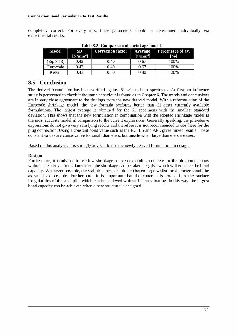
Comparison Bond Formulation to Test Results
71
completely correct. For every mix, these parameters should be determined individually via
experimental results.
Table 8.2: Comparison of shrinkage models.
Model SD
[N/mm2]
Correction factor Average
[N/mm2]
Percentage of av.
[%]
(Eq. 8.13) 0.42 0.40 0.67 100%
Eurocode 0.42 0.40 0.67 100%
Kelvin 0.43 0.60 0.80 120%
Conclusion 8.5
The derived formulation has been verified against 61 selected test specimens. At first, an influence
study is performed to check if the same behaviour is found as in Chapter 6. The trends and conclusions
are in very close agreement to the findings from the new derived model. With a reformulation of the
Eurocode shrinkage model, the new formula performs better than all other currently available
formulations. The largest average is obtained for the 61 specimens with the smallest standard
deviation. This shows that the new formulation in combination with the adopted shrinkage model is
the most accurate model in comparison to the current expressions. Generally speaking, the pile-sleeve
expressions do not give very satisfying results and therefore it is not recommended to use these for the
plug connection. Using a constant bond value such as the EC, BS and API, gives mixed results. These
constant values are conservative for small diameters, but unsafe when large diameters are used.
Based on this analysis, it is strongly advised to use the newly derived formulation in design.
Design:
Furthermore, it is advised to use low shrinkage or even expanding concrete for the plug connections
without shear keys. In the latter case, the shrinkage can be taken negative which will enhance the bond
capacity. Whenever possible, the wall thickness should be chosen large whilst the diameter should be
as small as possible. Furthermore, it is important that the concrete is forced into the surface
irregularities of the steel pile, which can be achieved with sufficient vibrating. In this way, the largest
bond capacity can be achieved when a new structure is designed.
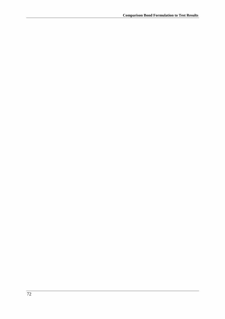
Comparison Bond Formulation to Test Results
72
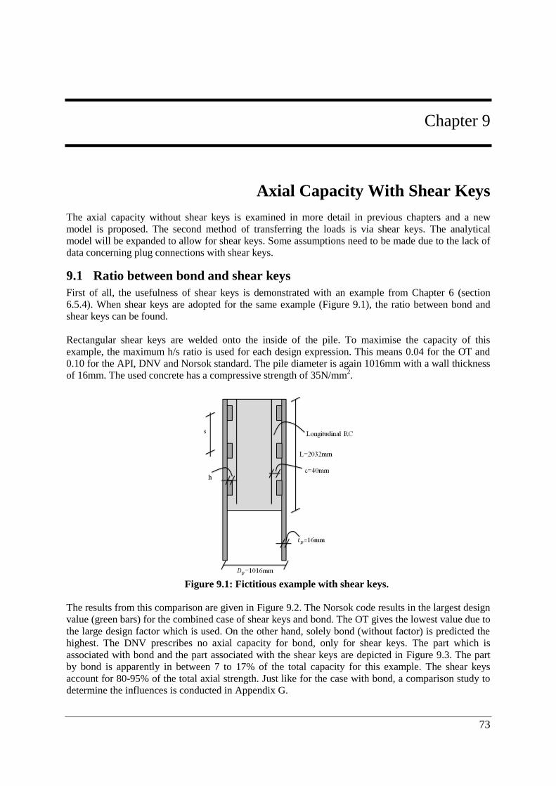
73
Chapter 9
9. Axial Capacity With Shear Keys
The axial capacity without shear keys is examined in more detail in previous chapters and a new
model is proposed. The second method of transferring the loads is via shear keys. The analytical
model will be expanded to allow for shear keys. Some assumptions need to be made due to the lack of
data concerning plug connections with shear keys.
Ratio between bond and shear keys 9.1
First of all, the usefulness of shear keys is demonstrated with an example from Chapter 6 (section
6.5.4). When shear keys are adopted for the same example (Figure 9.1), the ratio between bond and
shear keys can be found.
Rectangular shear keys are welded onto the inside of the pile. To maximise the capacity of this
example, the maximum h/s ratio is used for each design expression. This means 0.04 for the OT and
0.10 for the API, DNV and Norsok standard. The pile diameter is again 1016mm with a wall thickness
of 16mm. The used concrete has a compressive strength of 35N/mm2.
Figure 9.1: Fictitious example with shear keys.
The results from this comparison are given in Figure 9.2. The Norsok code results in the largest design
value (green bars) for the combined case of shear keys and bond. The OT gives the lowest value due to
the large design factor which is used. On the other hand, solely bond (without factor) is predicted the
highest. The DNV prescribes no axial capacity for bond, only for shear keys. The part which is
associated with bond and the part associated with the shear keys are depicted in Figure 9.3. The part
by bond is apparently in between 7 to 17% of the total capacity for this example. The shear keys
account for 80-95% of the total axial strength. Just like for the case with bond, a comparison study to
determine the influences is conducted in Appendix G.
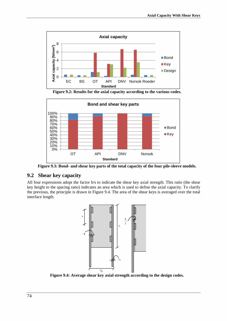
Axial Capacity With Shear Keys
74
Figure 9.2: Results for the axial capacity according to the various codes.
Figure 9.3: Bond- and shear key parts of the total capacity of the four pile-sleeve models.
Shear key capacity 9.2
All four expressions adopt the factor h/s to indicate the shear key axial strength. This ratio (the shear
key height to the spacing ratio) indicates an area which is used to define the axial capacity. To clarify
the previous, the principle is drawn in Figure 9.4. The area of the shear keys is averaged over the total
interface length.
Figure 9.4: Average shear key axial strength according to the design codes.
0
2
4
6
8
EC BS OT API DNV Norsok RoederAx
ial
ca
pa
cit
y [
N/m
m2]
Standard
Axial capacity
Bond
Key
Design
0%10%20%30%40%50%60%70%80%90%
100%
OT API DNV Norsok
Standard
Bond and shear key parts
Bond
Key
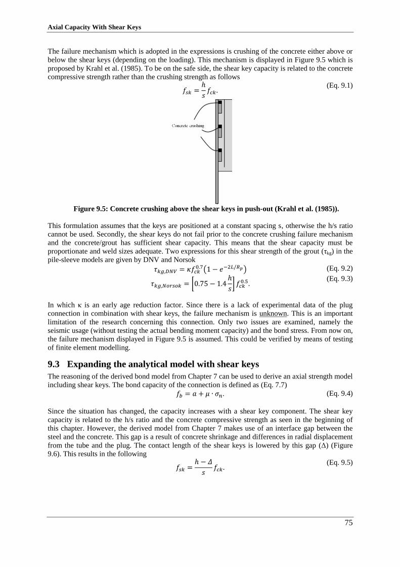
Axial Capacity With Shear Keys
75
The failure mechanism which is adopted in the expressions is crushing of the concrete either above or
below the shear keys (depending on the loading). This mechanism is displayed in Figure 9.5 which is
proposed by Krahl et al. (1985). To be on the safe side, the shear key capacity is related to the concrete
compressive strength rather than the crushing strength as follows
𝑓𝑠𝑘 =
ℎ
𝑠𝑓𝑐𝑘.
(Eq. 9.1)
Figure 9.5: Concrete crushing above the shear keys in push-out (Krahl et al. (1985)).
This formulation assumes that the keys are positioned at a constant spacing s, otherwise the h/s ratio
cannot be used. Secondly, the shear keys do not fail prior to the concrete crushing failure mechanism
and the concrete/grout has sufficient shear capacity. This means that the shear capacity must be
proportionate and weld sizes adequate. Two expressions for this shear strength of the grout (τkg) in the
pile-sleeve models are given by DNV and Norsok
𝜏𝑘𝑔,𝐷𝑁𝑉 = 𝜅𝑓𝑐𝑘0.7(1 − 𝑒−2𝐿/𝑅𝑝) (Eq. 9.2)
𝜏𝑘𝑔,𝑁𝑜𝑟𝑠𝑜𝑘 = [0.75 − 1.4
ℎ
𝑠] 𝑓𝑐𝑘
0.5. (Eq. 9.3)
In which κ is an early age reduction factor. Since there is a lack of experimental data of the plug
connection in combination with shear keys, the failure mechanism is unknown. This is an important
limitation of the research concerning this connection. Only two issues are examined, namely the
seismic usage (without testing the actual bending moment capacity) and the bond stress. From now on,
the failure mechanism displayed in Figure 9.5 is assumed. This could be verified by means of testing
of finite element modelling.
Expanding the analytical model with shear keys 9.3
The reasoning of the derived bond model from Chapter 7 can be used to derive an axial strength model
including shear keys. The bond capacity of the connection is defined as (Eq. 7.7)
𝑓𝑏 = 𝑎 + 𝜇 ∙ 𝜎𝑛. (Eq. 9.4)
Since the situation has changed, the capacity increases with a shear key component. The shear key
capacity is related to the h/s ratio and the concrete compressive strength as seen in the beginning of
this chapter. However, the derived model from Chapter 7 makes use of an interface gap between the
steel and the concrete. This gap is a result of concrete shrinkage and differences in radial displacement
from the tube and the plug. The contact length of the shear keys is lowered by this gap (Δ) (Figure
9.6). This results in the following
𝑓𝑠𝑘 =
ℎ − 𝛥
𝑠𝑓𝑐𝑘.
(Eq. 9.5)
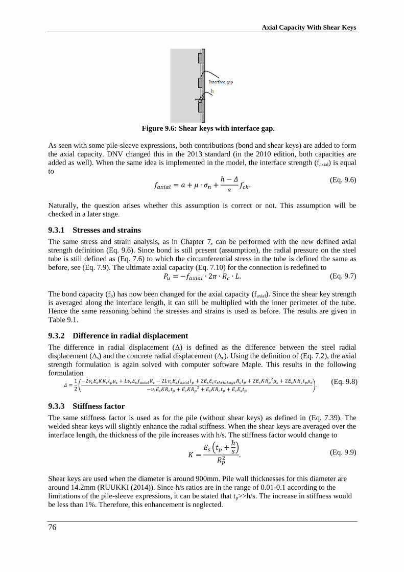
Axial Capacity With Shear Keys
76
Figure 9.6: Shear keys with interface gap.
As seen with some pile-sleeve expressions, both contributions (bond and shear keys) are added to form
the axial capacity. DNV changed this in the 2013 standard (in the 2010 edition, both capacities are
added as well). When the same idea is implemented in the model, the interface strength (faxial) is equal
to
𝑓𝑎𝑥𝑖𝑎𝑙 = 𝑎 + 𝜇 ∙ 𝜎𝑛 +
ℎ − 𝛥
𝑠𝑓𝑐𝑘.
(Eq. 9.6)
Naturally, the question arises whether this assumption is correct or not. This assumption will be
checked in a later stage.
9.3.1 Stresses and strains
The same stress and strain analysis, as in Chapter 7, can be performed with the new defined axial
strength definition (Eq. 9.6). Since bond is still present (assumption), the radial pressure on the steel
tube is still defined as (Eq. 7.6) to which the circumferential stress in the tube is defined the same as
before, see (Eq. 7.9). The ultimate axial capacity (Eq. 7.10) for the connection is redefined to
𝑃𝑢 = −𝑓𝑎𝑥𝑖𝑎𝑙 ∙ 2𝜋 ∙ 𝑅𝑐 ∙ 𝐿. (Eq. 9.7)
The bond capacity (fb) has now been changed for the axial capacity (faxial). Since the shear key strength
is averaged along the interface length, it can still be multiplied with the inner perimeter of the tube.
Hence the same reasoning behind the stresses and strains is used as before. The results are given in
Table 9.1.
9.3.2 Difference in radial displacement
The difference in radial displacement (Δ) is defined as the difference between the steel radial
displacement (Δs) and the concrete radial displacement (Δc). Using the definition of (Eq. 7.2), the axial
strength formulation is again solved with computer software Maple. This results in the following
formulation
𝛥 =1
2(−2𝑣𝑐𝐸𝑠𝐾𝑅𝑐𝑡𝑝𝜇𝑠 + 𝐿𝑣𝑠𝐸𝑐𝑓𝑎𝑥𝑖𝑎𝑙𝑅𝑐 − 2𝐿𝑣𝑐𝐸𝑠𝑓𝑎𝑥𝑖𝑎𝑙𝑡𝑝 + 2𝐸𝑠𝐸𝑐휀𝑠ℎ𝑟𝑖𝑛𝑘𝑎𝑔𝑒𝑅𝑐𝑡𝑝 + 2𝐸𝑐𝐾𝑅𝑝
2𝜇𝑠 + 2𝐸𝑠𝐾𝑅𝑐𝑡𝑝𝜇𝑠
−𝑣𝑐𝐸𝑠𝐾𝑅𝑐𝑡𝑝 + 𝐸𝑐𝐾𝑅𝑝2 + 𝐸𝑠𝐾𝑅𝑐𝑡𝑝 + 𝐸𝑐𝐸𝑠𝑡𝑝
). (Eq. 9.8)
9.3.3 Stiffness factor
The same stiffness factor is used as for the pile (without shear keys) as defined in (Eq. 7.39). The
welded shear keys will slightly enhance the radial stiffness. When the shear keys are averaged over the
interface length, the thickness of the pile increases with h/s. The stiffness factor would change to
𝐾 =𝐸𝑠 (𝑡𝑝 +
ℎ𝑠)
𝑅𝑝2 .
(Eq. 9.9)
Shear keys are used when the diameter is around 900mm. Pile wall thicknesses for this diameter are
around 14.2mm (RUUKKI (2014)). Since h/s ratios are in the range of 0.01-0.1 according to the
limitations of the pile-sleeve expressions, it can be stated that tp>>h/s. The increase in stiffness would
be less than 1%. Therefore, this enhancement is neglected.
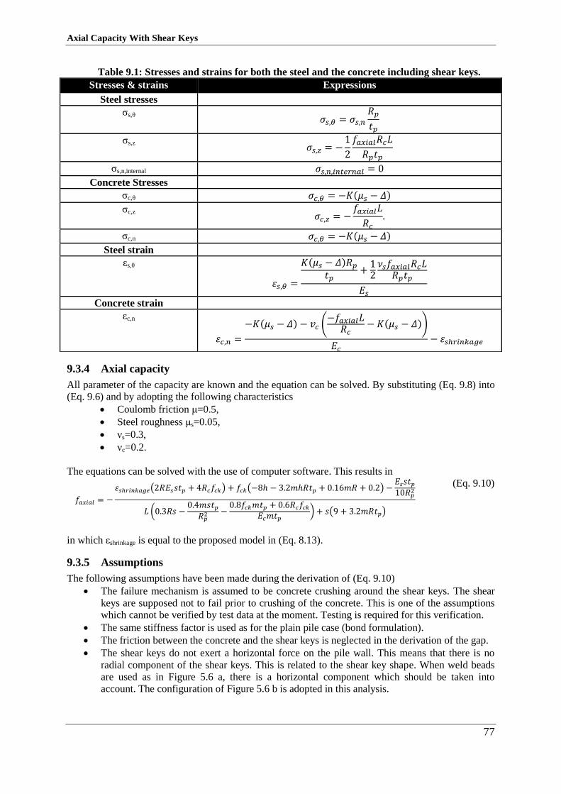
Axial Capacity With Shear Keys
77
Table 9.1: Stresses and strains for both the steel and the concrete including shear keys.
9.3.4 Axial capacity
All parameter of the capacity are known and the equation can be solved. By substituting (Eq. 9.8) into
(Eq. 9.6) and by adopting the following characteristics
Coulomb friction μ=0.5,
Steel roughness μs=0.05,
νs=0.3,
νc=0.2.
The equations can be solved with the use of computer software. This results in
𝑓𝑎𝑥𝑖𝑎𝑙 = −
휀𝑠ℎ𝑟𝑖𝑛𝑘𝑎𝑔𝑒(2𝑅𝐸𝑠𝑠𝑡𝑝 + 4𝑅𝑐𝑓𝑐𝑘) + 𝑓𝑐𝑘(−8ℎ − 3.2𝑚ℎ𝑅𝑡𝑝 + 0.16𝑚𝑅 + 0.2) −𝐸𝑠𝑠𝑡𝑝10𝑅𝑝
2
𝐿 (0.3𝑅𝑠 −0.4𝑚𝑠𝑡𝑝𝑅𝑝2 −
0.8𝑓𝑐𝑘𝑚𝑡𝑝 + 0.6𝑅𝑐𝑓𝑐𝑘𝐸𝑐𝑚𝑡𝑝
) + 𝑠(9 + 3.2𝑚𝑅𝑡𝑝)
(Eq. 9.10)
in which εshrinkage is equal to the proposed model in (Eq. 8.13).
9.3.5 Assumptions
The following assumptions have been made during the derivation of (Eq. 9.10)
The failure mechanism is assumed to be concrete crushing around the shear keys. The shear
keys are supposed not to fail prior to crushing of the concrete. This is one of the assumptions
which cannot be verified by test data at the moment. Testing is required for this verification.
The same stiffness factor is used as for the plain pile case (bond formulation).
The friction between the concrete and the shear keys is neglected in the derivation of the gap.
The shear keys do not exert a horizontal force on the pile wall. This means that there is no
radial component of the shear keys. This is related to the shear key shape. When weld beads
are used as in Figure 5.6 a, there is a horizontal component which should be taken into
account. The configuration of Figure 5.6 b is adopted in this analysis.
Stresses & strains Expressions
Steel stresses
σs,θ 𝜎𝑠,𝜃 = 𝜎𝑠,𝑛
𝑅𝑝𝑡𝑝
σs,z 𝜎𝑠,𝑧 = −
1
2
𝑓𝑎𝑥𝑖𝑎𝑙𝑅𝑐𝐿
𝑅𝑝𝑡𝑝
σs,n,internal 𝜎𝑠,𝑛,𝑖𝑛𝑡𝑒𝑟𝑛𝑎𝑙 = 0
Concrete Stresses
σc,θ 𝜎𝑐,𝜃 = −𝐾(𝜇𝑠 − 𝛥)
σc,z 𝜎𝑐,𝑧 = −
𝑓𝑎𝑥𝑖𝑎𝑙𝐿
𝑅𝑐.
σc,n 𝜎𝑐,𝜃 = −𝐾(𝜇𝑠 − 𝛥)
Steel strain
εs,θ
휀𝑠,𝜃 =
𝐾(𝜇𝑠 − 𝛥)𝑅𝑝𝑡𝑝
+12𝜈𝑠𝑓𝑎𝑥𝑖𝑎𝑙𝑅𝑐𝐿𝑅𝑝𝑡𝑝
𝐸𝑠
Concrete strain
εc,n
휀𝑐,𝑛 =
−𝐾(𝜇𝑠 − 𝛥) − 𝑣𝑐 (−𝑓𝑎𝑥𝑖𝑎𝑙𝐿𝑅𝑐
− 𝐾(𝜇𝑠 − 𝛥))
𝐸𝑐− 휀𝑠ℎ𝑟𝑖𝑛𝑘𝑎𝑔𝑒
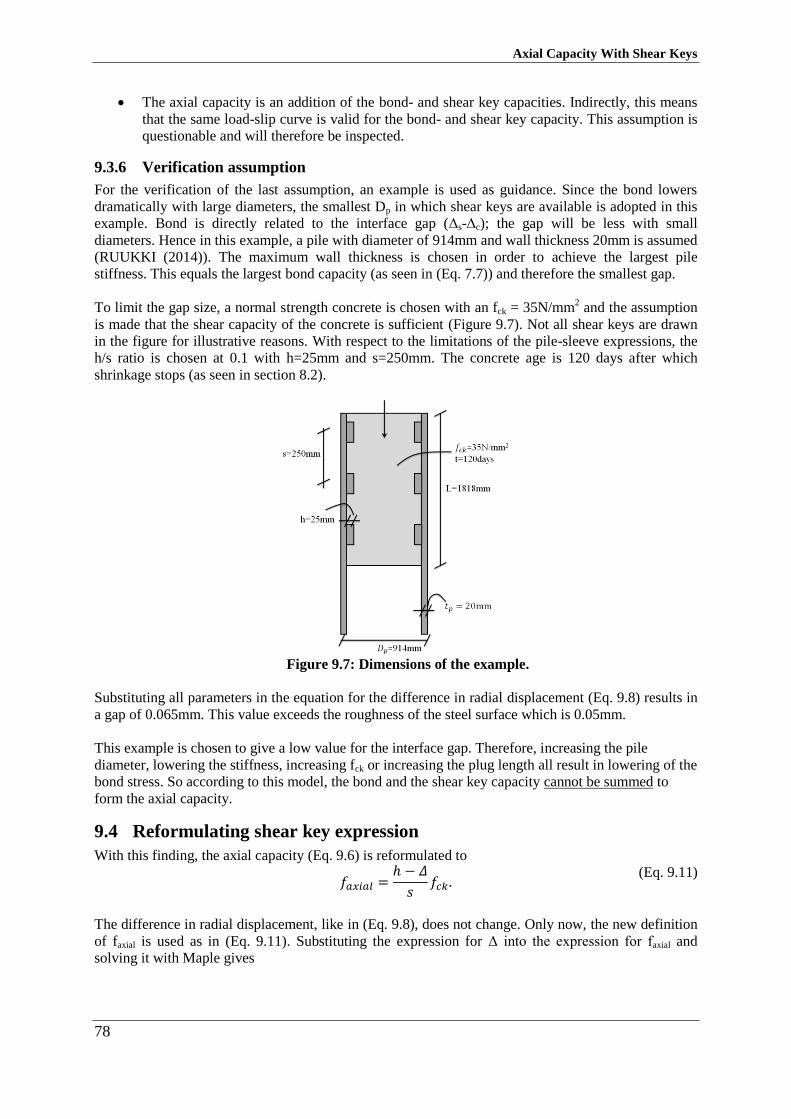
Axial Capacity With Shear Keys
78
The axial capacity is an addition of the bond- and shear key capacities. Indirectly, this means
that the same load-slip curve is valid for the bond- and shear key capacity. This assumption is
questionable and will therefore be inspected.
9.3.6 Verification assumption
For the verification of the last assumption, an example is used as guidance. Since the bond lowers
dramatically with large diameters, the smallest Dp in which shear keys are available is adopted in this
example. Bond is directly related to the interface gap (Δs-Δc); the gap will be less with small
diameters. Hence in this example, a pile with diameter of 914mm and wall thickness 20mm is assumed
(RUUKKI (2014)). The maximum wall thickness is chosen in order to achieve the largest pile
stiffness. This equals the largest bond capacity (as seen in (Eq. 7.7)) and therefore the smallest gap.
To limit the gap size, a normal strength concrete is chosen with an fck = 35N/mm2 and the assumption
is made that the shear capacity of the concrete is sufficient (Figure 9.7). Not all shear keys are drawn
in the figure for illustrative reasons. With respect to the limitations of the pile-sleeve expressions, the
h/s ratio is chosen at 0.1 with h=25mm and s=250mm. The concrete age is 120 days after which
shrinkage stops (as seen in section 8.2).
Figure 9.7: Dimensions of the example.
Substituting all parameters in the equation for the difference in radial displacement (Eq. 9.8) results in
a gap of 0.065mm. This value exceeds the roughness of the steel surface which is 0.05mm.
This example is chosen to give a low value for the interface gap. Therefore, increasing the pile
diameter, lowering the stiffness, increasing fck or increasing the plug length all result in lowering of the
bond stress. So according to this model, the bond and the shear key capacity cannot be summed to
form the axial capacity.
Reformulating shear key expression 9.4
With this finding, the axial capacity (Eq. 9.6) is reformulated to
𝑓𝑎𝑥𝑖𝑎𝑙 =
ℎ − 𝛥
𝑠𝑓𝑐𝑘.
(Eq. 9.11)
The difference in radial displacement, like in (Eq. 9.8), does not change. Only now, the new definition
of faxial is used as in (Eq. 9.11). Substituting the expression for Δ into the expression for faxial and
solving it with Maple gives
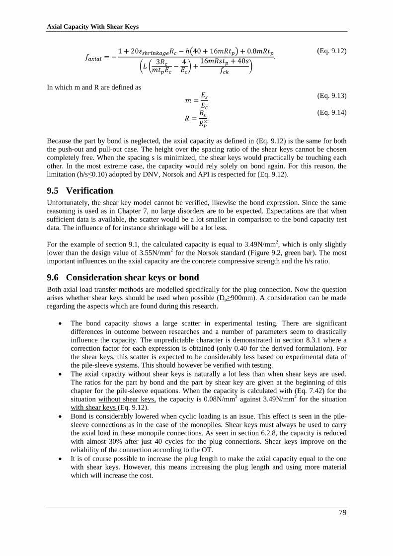
Axial Capacity With Shear Keys
79
𝑓𝑎𝑥𝑖𝑎𝑙 = −
1 + 20휀𝑠ℎ𝑟𝑖𝑛𝑘𝑎𝑔𝑒𝑅𝑐 − ℎ(40 + 16𝑚𝑅𝑡𝑝) + 0.8𝑚𝑅𝑡𝑝
(𝐿 (3𝑅𝑐𝑚𝑡𝑝𝐸𝑐
−4𝐸𝑐) +
16𝑚𝑅𝑠𝑡𝑝 + 40𝑠𝑓𝑐𝑘
)
. (Eq. 9.12)
In which m and R are defined as
𝑚 =
𝐸𝑠𝐸𝑐
𝑅 =𝑅𝑐
𝑅𝑝2.
(Eq. 9.13)
(Eq. 9.14)
Because the part by bond is neglected, the axial capacity as defined in (Eq. 9.12) is the same for both
the push-out and pull-out case. The height over the spacing ratio of the shear keys cannot be chosen
completely free. When the spacing s is minimized, the shear keys would practically be touching each
other. In the most extreme case, the capacity would rely solely on bond again. For this reason, the
limitation (h/s≤0.10) adopted by DNV, Norsok and API is respected for (Eq. 9.12).
Verification 9.5
Unfortunately, the shear key model cannot be verified, likewise the bond expression. Since the same
reasoning is used as in Chapter 7, no large disorders are to be expected. Expectations are that when
sufficient data is available, the scatter would be a lot smaller in comparison to the bond capacity test
data. The influence of for instance shrinkage will be a lot less.
For the example of section 9.1, the calculated capacity is equal to 3.49N/mm2, which is only slightly
lower than the design value of 3.55N/mm2 for the Norsok standard (Figure 9.2, green bar). The most
important influences on the axial capacity are the concrete compressive strength and the h/s ratio.
Consideration shear keys or bond 9.6
Both axial load transfer methods are modelled specifically for the plug connection. Now the question
arises whether shear keys should be used when possible (Dp≥900mm). A consideration can be made
regarding the aspects which are found during this research.
The bond capacity shows a large scatter in experimental testing. There are significant
differences in outcome between researches and a number of parameters seem to drastically
influence the capacity. The unpredictable character is demonstrated in section 8.3.1 where a
correction factor for each expression is obtained (only 0.40 for the derived formulation). For
the shear keys, this scatter is expected to be considerably less based on experimental data of
the pile-sleeve systems. This should however be verified with testing.
The axial capacity without shear keys is naturally a lot less than when shear keys are used.
The ratios for the part by bond and the part by shear key are given at the beginning of this
chapter for the pile-sleeve equations. When the capacity is calculated with (Eq. 7.42) for the
situation without shear keys, the capacity is 0.08N/mm2 against 3.49N/mm
2 for the situation
with shear keys (Eq. 9.12).
Bond is considerably lowered when cyclic loading is an issue. This effect is seen in the pile-
sleeve connections as in the case of the monopiles. Shear keys must always be used to carry
the axial load in these monopile connections. As seen in section 6.2.8, the capacity is reduced
with almost 30% after just 40 cycles for the plug connections. Shear keys improve on the
reliability of the connection according to the OT.
It is of course possible to increase the plug length to make the axial capacity equal to the one
with shear keys. However, this means increasing the plug length and using more material
which will increase the cost.
Axial Capacity With Shear Keys
80
The last bullet implies that a cost comparison should be made for the situation with and without shear
keys. For this analysis (Figure 9.8), the same pile as in the example of section 9.3.6 is used. For the
cost analysis, it is assumed that this connection is made at a location with relative high wages (west
European wages). The distance to suppliers is considered reasonable and all required labour and
materials are present within reasonable distances.
The smallest possible diameter of 914mm is adopted with a large wall thickness of 20mm (RUUKKI
(2014)). These values are chosen because the bond capacity will be the highest for this situation since
it drops dramatically with increasing diameters. The used plug length is equal to the minimal length of
1200mm. With the limitations in mind, the shear key height is 25mm and the width (w) equal to
40mm. The latter is chosen according to the API limitation. In total two shear keys are used which
result in an h/s ratio of 0.06. The used concrete is C35/45 at an age of 120 days.
For this example, an axial force (P) of 3000kN is assumed, which needs to be transferred from the
plug to the pile. For the plain plug connection (without shear keys), the interface length can be
determined with the given axial force. The bond multiplied with the area, should equal the exerted
axial force
𝑓𝑏 ∙ 2𝜋𝑅𝑐𝐿 = 𝑃. (Eq. 9.15)
Substituting the expression for fb (Eq. 7.45) and solving (Eq. 9.15) with respect to L gives
𝐿 =
16𝑃(5𝐸𝑐𝑅𝑝2 + 2𝐸𝑠𝑅𝑐𝑡𝑝
40𝜋𝐸𝑐𝐸𝑠휀𝑠ℎ𝑟𝑖𝑛𝑘𝑎𝑔𝑒𝑅𝑐2𝑡𝑝 − 2𝜋𝐸𝑐𝐸𝑠𝑅𝑐𝑡𝑝 + 3𝑃𝐸𝑐𝑅𝑐 − 4𝑃𝐸𝑠𝑡𝑝
. (Eq. 9.16)
Substituting all parameters gives the required plug length, which is equal to 6050mm.
Figure 9.8: Example with the given dimensions, on the left the option with shear keys and on
the right the option without shear keys.
9.6.1 Costs comparison
The main differences in costs between the two options arise due to two reasons:
Welding of the shear keys and the required steel,
The amount of concrete which is used with the associated reinforcement and transportation
costs.
Axial Capacity With Shear Keys
81
Assumptions for this comparison are
Formwork for casting the plug for both cases is equally expensive,
20 plugs a day can be casted for the one with shear keys and 15 plugs for the plain connection,
200kg reinforcement is used per m3 concrete.
Labour costs €35/hr except for welders, which cost €50/hr.
Concrete costs €150/m3 (including additional pumping charges of €10/m
3) and steel €1500/m
3.
Transportation is done with a pontoon propelled by a tug boat.
With the given assumptions, the costs per plug connection are estimated in Appendix H. When the
costs for the plug with shear keys are set to 100%, the costs for the plug without (plain connection) are
approximately 104% for the axial load of 3000kN. With an axial load of 2500kN, the plain plug is
only 91% of the costs of the one with shear keys, since the plug length is less.
Like seen in section 4.4.4, the costs are closely related to the situation at hand. Distance to suppliers,
availability of certified welders, available equipment, labour costs etc. are aspects which should be
taken into account. A statement regarding which solution to adopt in general based on the costs,
cannot be made. A cost comparison should be made for every project to determine the most favourable
option of the two. Furthermore, it is noted that the costs which are presented are only the direct
material and labour costs. The profit margin, costs for potential risks, and general company costs are
not included.
Since the difference in costs is rather limited, it is advised to use shear keys whenever possible. The
problem of deterioration of the bond capacity due to cyclic loading is excluded from happening in this
manner. The long term behaviour of the connection will be secured.
Conclusion 9.7
In this chapter, a new equation is proposed for the plug connection with shear keys. Due to the lack of
test data, this formulation cannot be verified in the same way as with the bond model. When sufficient
data is present, the formulation will most probably give satisfactory results because the same
reasoning is used as with bond. One of the most important conclusions is that the bond and shear key
part cannot be summed according to the used methodology. The gap exceeds the surface roughness
and therefore the bond is broken.
A cost analysis should be made for each project to determine the cheapest solution. Shear keys are
advantageous over bond when cyclic loading is considered. Since the difference in costs between the
two options is rather limited, it is advised to use shear keys when possible to exclude the cyclic
loading effect.
Design:
For the design of the plug with shear keys, it is advised to use an adequate dimensioned reinforcement
net to provide the required shear capacity for the plug itself. The concrete compressive strength has a
large influence on the shear key capacity, so usage of high strength concrete is advised. Furthermore,
the keys should be placed with a constant distance and with an appropriate spacing. The maximum h/s
ratio of 0.10 is therefore respected.
Axial Capacity With Shear Keys
82
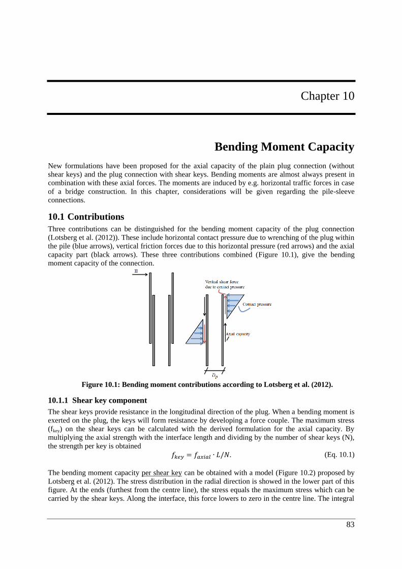
83
Chapter 10
10. Bending Moment Capacity
New formulations have been proposed for the axial capacity of the plain plug connection (without
shear keys) and the plug connection with shear keys. Bending moments are almost always present in
combination with these axial forces. The moments are induced by e.g. horizontal traffic forces in case
of a bridge construction. In this chapter, considerations will be given regarding the pile-sleeve
connections.
Contributions 10.1
Three contributions can be distinguished for the bending moment capacity of the plug connection
(Lotsberg et al. (2012)). These include horizontal contact pressure due to wrenching of the plug within
the pile (blue arrows), vertical friction forces due to this horizontal pressure (red arrows) and the axial
capacity part (black arrows). These three contributions combined (Figure 10.1), give the bending
moment capacity of the connection.
Figure 10.1: Bending moment contributions according to Lotsberg et al. (2012).
10.1.1 Shear key component
The shear keys provide resistance in the longitudinal direction of the plug. When a bending moment is
exerted on the plug, the keys will form resistance by developing a force couple. The maximum stress
(fkey) on the shear keys can be calculated with the derived formulation for the axial capacity. By
multiplying the axial strength with the interface length and dividing by the number of shear keys (N),
the strength per key is obtained
𝑓𝑘𝑒𝑦 = 𝑓𝑎𝑥𝑖𝑎𝑙 ∙ 𝐿/𝑁. (Eq. 10.1)
The bending moment capacity per shear key can be obtained with a model (Figure 10.2) proposed by
Lotsberg et al. (2012). The stress distribution in the radial direction is showed in the lower part of this
figure. At the ends (furthest from the centre line), the stress equals the maximum stress which can be
carried by the shear keys. Along the interface, this force lowers to zero in the centre line. The integral
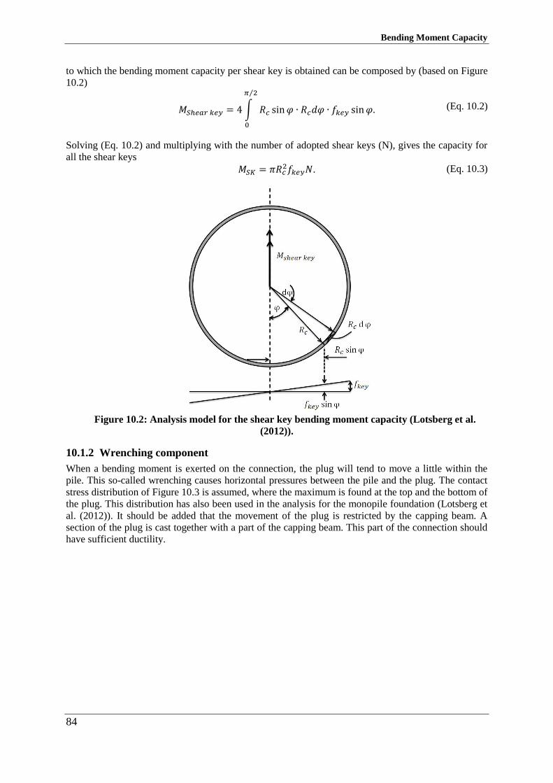
Bending Moment Capacity
84
to which the bending moment capacity per shear key is obtained can be composed by (based on Figure
10.2)
𝑀𝑆ℎ𝑒𝑎𝑟 𝑘𝑒𝑦 = 4 ∫ 𝑅𝑐 sin𝜑 ∙ 𝑅𝑐𝑑𝜑 ∙ 𝑓𝑘𝑒𝑦 sin𝜑.
𝜋 2⁄
0
(Eq. 10.2)
Solving (Eq. 10.2) and multiplying with the number of adopted shear keys (N), gives the capacity for
all the shear keys
𝑀𝑆𝐾 = 𝜋𝑅𝑐2𝑓𝑘𝑒𝑦𝑁. (Eq. 10.3)
Figure 10.2: Analysis model for the shear key bending moment capacity (Lotsberg et al.
(2012)).
10.1.2 Wrenching component
When a bending moment is exerted on the connection, the plug will tend to move a little within the
pile. This so-called wrenching causes horizontal pressures between the pile and the plug. The contact
stress distribution of Figure 10.3 is assumed, where the maximum is found at the top and the bottom of
the plug. This distribution has also been used in the analysis for the monopile foundation (Lotsberg et
al. (2012)). It should be added that the movement of the plug is restricted by the capping beam. A
section of the plug is cast together with a part of the capping beam. This part of the connection should
have sufficient ductility.
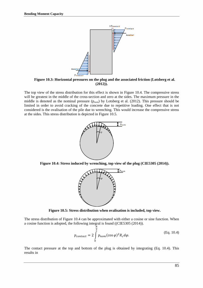
Bending Moment Capacity
85
Figure 10.3: Horizontal pressures on the plug and the associated friction (Lotsberg et al.
(2012)).
The top view of the stress distribution for this effect is shown in Figure 10.4. The compressive stress
will be greatest in the middle of the cross-section and zero at the sides. The maximum pressure in the
middle is denoted as the nominal pressure (pnom) by Lotsberg et al. (2012). This pressure should be
limited in order to avoid cracking of the concrete due to repetitive loading. One effect that is not
considered is the ovalisation of the pile due to wrenching. This would increase the compressive stress
at the sides. This stress distribution is depicted in Figure 10.5.
Figure 10.4: Stress induced by wrenching, top view of the plug (CIE5305 (2014)).
Figure 10.5: Stress distribution when ovalisation is included, top view.
The stress distribution of Figure 10.4 can be approximated with either a cosine or sine function. When
a cosine function is adopted, the following integral is found ((CIE5305 (2014)).
𝑝𝑐𝑜𝑛𝑡𝑎𝑐𝑡 = 2∫𝑝𝑛𝑜𝑚(cos𝜑)2𝑅𝑐𝑑𝜑.
𝜋2
0
(Eq. 10.4)
The contact pressure at the top and bottom of the plug is obtained by integrating (Eq. 10.4). This
results in
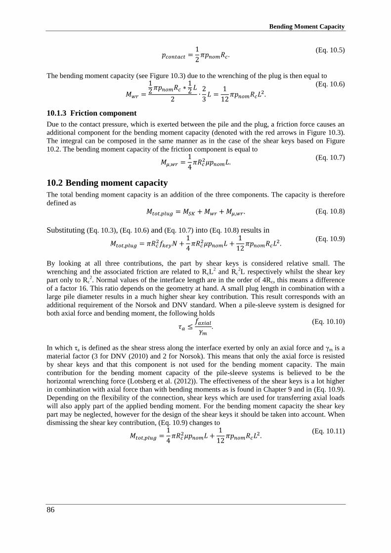
Bending Moment Capacity
86
𝑝𝑐𝑜𝑛𝑡𝑎𝑐𝑡 =
1
2𝜋𝑝𝑛𝑜𝑚𝑅𝑐 .
(Eq. 10.5)
The bending moment capacity (see Figure 10.3) due to the wrenching of the plug is then equal to
𝑀𝑤𝑟 =
12𝜋𝑝𝑛𝑜𝑚𝑅𝑐 ∗
12𝐿
2∙2
3𝐿 =
1
12𝜋𝑝𝑛𝑜𝑚𝑅𝑐𝐿
2.
(Eq. 10.6)
10.1.3 Friction component
Due to the contact pressure, which is exerted between the pile and the plug, a friction force causes an
additional component for the bending moment capacity (denoted with the red arrows in Figure 10.3).
The integral can be composed in the same manner as in the case of the shear keys based on Figure
10.2. The bending moment capacity of the friction component is equal to
𝑀𝜇,𝑤𝑟 =
1
4𝜋𝑅𝑐
2𝜇𝑝𝑛𝑜𝑚𝐿. (Eq. 10.7)
Bending moment capacity 10.2
The total bending moment capacity is an addition of the three components. The capacity is therefore
defined as
𝑀𝑡𝑜𝑡,𝑝𝑙𝑢𝑔 = 𝑀𝑆𝐾 +𝑀𝑤𝑟 +𝑀𝜇,𝑤𝑟. (Eq. 10.8)
Substituting (Eq. 10.3), (Eq. 10.6) and (Eq. 10.7) into (Eq. 10.8) results in
𝑀𝑡𝑜𝑡,𝑝𝑙𝑢𝑔 = 𝜋𝑅𝑐
2𝑓𝑘𝑒𝑦𝑁 +1
4𝜋𝑅𝑐
2𝜇𝑝𝑛𝑜𝑚𝐿 +1
12𝜋𝑝𝑛𝑜𝑚𝑅𝑐𝐿
2. (Eq. 10.9)
By looking at all three contributions, the part by shear keys is considered relative small. The
wrenching and the associated friction are related to RcL2 and Rc
2L respectively whilst the shear key
part only to Rc2. Normal values of the interface length are in the order of 4Rc, this means a difference
of a factor 16. This ratio depends on the geometry at hand. A small plug length in combination with a
large pile diameter results in a much higher shear key contribution. This result corresponds with an
additional requirement of the Norsok and DNV standard. When a pile-sleeve system is designed for
both axial force and bending moment, the following holds
𝜏𝑎 ≤
𝑓𝑎𝑥𝑖𝑎𝑙𝛾𝑚
. (Eq. 10.10)
In which τa is defined as the shear stress along the interface exerted by only an axial force and γm is a
material factor (3 for DNV (2010) and 2 for Norsok). This means that only the axial force is resisted
by shear keys and that this component is not used for the bending moment capacity. The main
contribution for the bending moment capacity of the pile-sleeve systems is believed to be the
horizontal wrenching force (Lotsberg et al. (2012)). The effectiveness of the shear keys is a lot higher
in combination with axial force than with bending moments as is found in Chapter 9 and in (Eq. 10.9).
Depending on the flexibility of the connection, shear keys which are used for transferring axial loads
will also apply part of the applied bending moment. For the bending moment capacity the shear key
part may be neglected, however for the design of the shear keys it should be taken into account. When
dismissing the shear key contribution, (Eq. 10.9) changes to
𝑀𝑡𝑜𝑡,𝑝𝑙𝑢𝑔 =
1
4𝜋𝑅𝑐
2𝜇𝑝𝑛𝑜𝑚𝐿 +1
12𝜋𝑝𝑛𝑜𝑚𝑅𝑐𝐿
2. (Eq. 10.11)
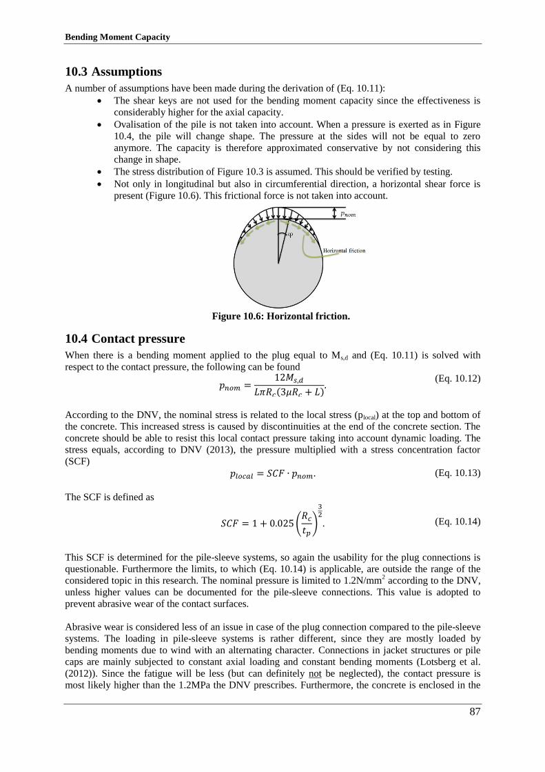
Bending Moment Capacity
87
Assumptions 10.3
A number of assumptions have been made during the derivation of (Eq. 10.11):
The shear keys are not used for the bending moment capacity since the effectiveness is
considerably higher for the axial capacity.
Ovalisation of the pile is not taken into account. When a pressure is exerted as in Figure
10.4, the pile will change shape. The pressure at the sides will not be equal to zero
anymore. The capacity is therefore approximated conservative by not considering this
change in shape.
The stress distribution of Figure 10.3 is assumed. This should be verified by testing.
Not only in longitudinal but also in circumferential direction, a horizontal shear force is
present (Figure 10.6). This frictional force is not taken into account.
Figure 10.6: Horizontal friction.
Contact pressure 10.4
When there is a bending moment applied to the plug equal to Ms,d and (Eq. 10.11) is solved with
respect to the contact pressure, the following can be found
𝑝𝑛𝑜𝑚 =
12𝑀𝑠,𝑑𝐿𝜋𝑅𝑐(3𝜇𝑅𝑐 + 𝐿)
. (Eq. 10.12)
According to the DNV, the nominal stress is related to the local stress (plocal) at the top and bottom of
the concrete. This increased stress is caused by discontinuities at the end of the concrete section. The
concrete should be able to resist this local contact pressure taking into account dynamic loading. The
stress equals, according to DNV (2013), the pressure multiplied with a stress concentration factor
(SCF)
𝑝𝑙𝑜𝑐𝑎𝑙 = 𝑆𝐶𝐹 ∙ 𝑝𝑛𝑜𝑚. (Eq. 10.13)
The SCF is defined as
𝑆𝐶𝐹 = 1 + 0.025(𝑅𝑐𝑡𝑝)
32
.
(Eq. 10.14)
This SCF is determined for the pile-sleeve systems, so again the usability for the plug connections is
questionable. Furthermore the limits, to which (Eq. 10.14) is applicable, are outside the range of the
considered topic in this research. The nominal pressure is limited to 1.2N/mm2 according to the DNV,
unless higher values can be documented for the pile-sleeve connections. This value is adopted to
prevent abrasive wear of the contact surfaces.
Abrasive wear is considered less of an issue in case of the plug connection compared to the pile-sleeve
systems. The loading in pile-sleeve systems is rather different, since they are mostly loaded by
bending moments due to wind with an alternating character. Connections in jacket structures or pile
caps are mainly subjected to constant axial loading and constant bending moments (Lotsberg et al.
(2012)). Since the fatigue will be less (but can definitely not be neglected), the contact pressure is
most likely higher than the 1.2MPa the DNV prescribes. Furthermore, the concrete is enclosed in the
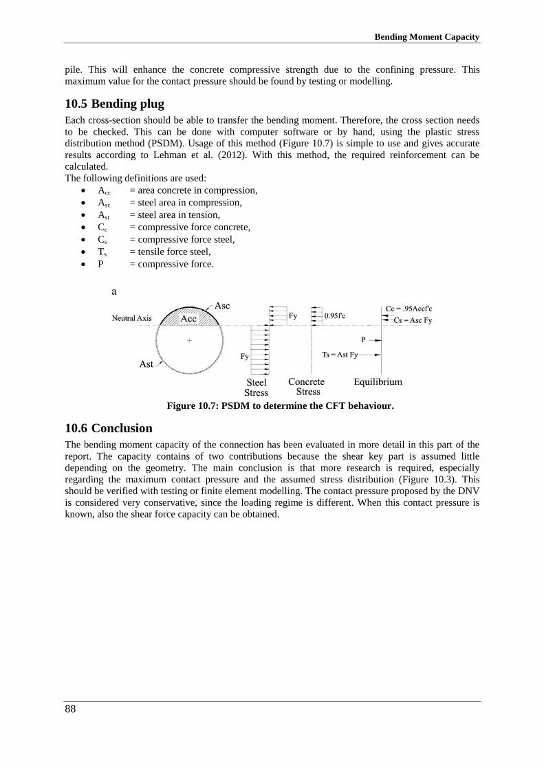
Bending Moment Capacity
88
pile. This will enhance the concrete compressive strength due to the confining pressure. This
maximum value for the contact pressure should be found by testing or modelling.
Bending plug 10.5
Each cross-section should be able to transfer the bending moment. Therefore, the cross section needs
to be checked. This can be done with computer software or by hand, using the plastic stress
distribution method (PSDM). Usage of this method (Figure 10.7) is simple to use and gives accurate
results according to Lehman et al. (2012). With this method, the required reinforcement can be
calculated.
The following definitions are used:
Acc = area concrete in compression,
Asc = steel area in compression,
Ast = steel area in tension,
Cc = compressive force concrete,
Cs = compressive force steel,
Ts = tensile force steel,
P = compressive force.
Figure 10.7: PSDM to determine the CFT behaviour.
Conclusion 10.6
The bending moment capacity of the connection has been evaluated in more detail in this part of the
report. The capacity contains of two contributions because the shear key part is assumed little
depending on the geometry. The main conclusion is that more research is required, especially
regarding the maximum contact pressure and the assumed stress distribution (Figure 10.3). This
should be verified with testing or finite element modelling. The contact pressure proposed by the DNV
is considered very conservative, since the loading regime is different. When this contact pressure is
known, also the shear force capacity can be obtained.
89
Chapter 11
11. Conclusions & Recommendations
The most important conclusions of this research are drawn in this chapter. The main research question
will be answered and recommendations for future research are formulated.
Conclusions 11.1
Various possible solutions for the steel pile to concrete element connection are developed over the
years. The embedded alternatives result in capping beam reinforcement problems and large concrete
elements due to punching shear. This is associated with constructability issues on site and an increase
of the costs due to the very dense reinforcement lay-out. The encased-fixed based detail suffers from
the same issues as the embedded connection types. Additionally, a lot of welding is required which
need to be performed on site.
Concluding from a trade-off analysis, the plug connection is less expensive, equally fast to make and
more durable in relation to the plate connection and the reinforcement welded to steel shell option. The
latter solution is dismissed, due to the many steps during production and the amount of required
welding on site. Furthermore, the plug connection is adopted in almost 90% of the cases. This latter
finding is based on experience and a proposed decision scheme. This decision scheme is subsequently
based on a list of possible influences on the connection design.
The plug connection can either be axially loaded in tension (pull-out) or compression (push-out). In
pull-out, the plug breaks at the tip of the longitudinal reinforcement bars. The push-out case is purely a
bond failure. Two axial transfer methods are possible, namely by bond or by shear keys. The most
influential parameters for bond are the geometry of the pile, concrete shrinkage and cyclic loading.
The latter gives a reduction up to 30% with only limited cycles.
Bond
Various bond formulations are available today based on pile sleeve-systems, constant values or linear
regression. All lack an empirical background. A new formulation is proposed based on the stresses and
strains of both the plug and the pile. Bond is defined as micro-friction, the adhesion part is assumed
zero. This new formulation coincides well with the found trends from literature. The main
disadvantage of the Kelvin shrinkage model is the required testing for each concrete mixture. The
shrinkage behaviour within the tubular piles is different than that of exposed concrete. Therefore, it is
concluded that a reformulation of the Eurocode shrinkage model is preferred.
This new formulation together with the chosen shrinkage model is verified with 61 test specimens.
The standard deviation equals 0.42N/mm2 which is regarded as large. The main reason is the large
scatter in the test data. With the correction factor of 0.40, the average bond for the 61 specimens is
equal to 0.67N/mm2. These numbers are put into perspective by testing the six currently available
formulations. All resulted in higher standard deviations and average values which are lower.
Therefore, it is concluded that the new formulation predicts best. Low shrinkage or even expanding
concrete should be used. Furthermore, it is not recommended to use the pile-sleeve expressions.
Conclusions & Recommendations
90
Shear keys
The bond and shear key capacities cannot be summed in the new shear key formulation. Furthermore,
there is a lack of experimental data of the plug connection in combination with shear keys. The new
formulation cannot be verified as is done with the new bond expression. Shear keys should be used
whenever possible due to the deterioration effect of cyclic loading on the bond capacity. The
difference in costs between the two options is rather limited depending on the specific situation.
The bending moment capacity contains two contributions, namely the wrenching effect and the
associated friction. The third possible contribution, shear keys, is only limited when common
geometry values are used. The maximum contact pressure is set to a maximum value based on cyclic
loading effects in pile-sleeve connections. This effect is expected to be less for the plug connections
and therefore this value can most probably be increased.
Research question 11.2
The findings of this research are used to answer the main research question, formulated at the
beginning of this report:
What is the best strategy of connecting a steel pipe pile to a concrete element in different near-
shore situations dealing with unknown/inconsistent factors and with respect to trade-off aspects
such as economy, durability and manufacturability?
The best strategy of connecting the pipe pile to a concrete element is by using the concrete plug
connection. This connection type can be used in all kinds of situations, can transfer high loads and is
relatively easy to construct. The costs of this connection are rather low and the durability of the
connection is good.
The main issues concerning the plug connection are the inconsistent design formulations for the bond
capacity and the lack of formulations for the axial capacity. These matters are addressed by
formulating new design expressions. The formulation for the bond capacity agrees better with test data
than any other currently available formulation. It is therefore highly recommended to use this new
equation in design.
Currently, formulations including shear keys are only available for pile-sleeve applications. Therefore,
there is a large need for shear key formulations for the plug connection. The analytical model is
expanded such that shear keys are adopted in the formulation. It is expected that as with the bond,
these values will coincide well with reality. This should however be verified. Finally, an expression
for the bending moment capacity is formulated. Before using this for design, certain assumptions need
to be checked.
Conclusions & Recommendations
91
Recommendations 11.3
Based on this research, the following recommendations for future research are formulated:
This research is focused on the load transfer from the plug to the pile. The top part of the
connection, namely the dowels connecting the plug to the concrete element, can be further
optimized.
Reinforcement in the plug can change the failure mode due to wedging effects. It is believed
that this effect increases the bond capacity of the connection. This should be determined in
more detail.
The effect of cyclic loading can be determined in more detail.
The plug connection should be tested in combination with shear keys. The assumed failure
mechanism should be checked. Subsequently, the proposed formulation of Chapter 9 can be
verified as done with the formulation for bond.
The maximum contact pressure should be verified with either testing or modelling.
The assumed stress distribution used to calculate the bending moment capacity should be
verified with experiments.
Conclusions & Recommendations
92
93
Bibliography
12. References
AASHTO (2012). ‘AASHTO LRFD Bridge, Design Specifications.’ American Association of State
Highway and Transportation Officials (AASHTO), 2012, ISBN 978-1-56051-523-4.
Al-Mahaidi, R., Grundy, P. and Bean, W. (1999). ‘Pullout Strength of Concrete Plugs in Tubular
Piles.’ Proceedings of the Ninth International Offshore and Polar Engineering Conference, Brest
France, May 1999, pp. 24-29.
Aly, T., Elchalakani, M., Thayalan, P. and Patnuikuni, I. (2009). ‘Incremental Collapse Treshold for
Pushout Resistance of Circular Concrete Filled Steel Tubular Columns.’ Journal of Constructional
Steel Research 66, Elsevier, 2010, pp. 11-18.
API (2003). ‘API Recommended Practice2A-LRFD.’ American Petroleum Institute (API), Chapter 4:
Grouted Pile-to-Structure Connections, pp. 79-80.
Arcelor Mittal (2010). ‘Spirally Welded Steel Pipes.’ Product Range, 2010.
BN (2015). Ballast Nedam (BN), Personal Communication.
Berg, L.M. (2014). ‘CFT Column-to-Cap Beam Connections for Accelerated Bridge Construction in
Seismic Regions.’ Master Thesis, Civil and Environmental Engineering, University of Washington.
Billington, C.J. and Lewis, H.G. (1978). ‘The Strength of Large Diameter Grouted Connections.’
Offshore Technology Conference, 10th Annual OTC 3083, Houston Texas.
Billington, C.J. and Tebbett, I.E. (1980). ‘The Basis for New Design Formulae for Grouted Jacket to
Pile Connections.’ Offshore Technology Conference, 12th Annual OTC, OTC 3788, Houston, Texas.
BSI (1999). ‘Steel, Concrete and Composite Bridges: Code of Practice for Design of Composite
Bridges.’ British Standard Institution (BSI), British Standard BS5400, London UK, pp. 29.
CIE5305 (2014). ‘Bored and Immersed Tunnels.’ Chapter 4: Bored Tunnels.
Chilvers, G.A. (1984). ‘Analysis of the Structural Behaviour of Grouted Pile/Sleeve Connections for
Offshore Structures.’ Thesis Submitted to the City University for the Degree of Doctor of Philosophy
in the Department of Civil Engineering.
DNV (2013). ‘Design of Offshore Wind Turbine Structures.’ Det Norske Veritas (DNV), Offshore
Standard, DNV-OS-J101.
Bibliography
94
ECS (2001). ‘NEN-EN12699: Adopted European Prestandard, Execution of Special Geotechnical
Work – Displacement Piles.’ NEN-EN12699, European Committee for Standardization (ECS),
Brussels Belgium.
ECS (2005). ‘Eurocode 1: Adopted European Prestandard.’ NEN-EN1991-1-4 European Committee
for Standardization (ECS), Brussels Belgium.
ECS (2007). ‘NEN-EN12944: Adopted European Prestandard.’ NEN-EN12944, European Committee
for Standardization (ECS), Brussels Belgium.
ECS (2008). ‘Eurocode 3: Adopted European Prestandard.’ NEN-EN1993-5 (en), European
Committee for Standardization (ECS), Brussels Belgium.
ECS (2011a). ‘Eurocode 0: Adopted European Prestandard.’ NEN-EN1990+A1+A1/C1,
European Committee for Standardization (ECS), Brussels, Belgium.
ECS (2011b). ‘Eurocode 2: Adopted European Prestandard.’ NEN-EN1992-1-1+C2, European
Committee for Standardization (ECS), Brussels Belgium.
ECS (2011c). ’Eurocode 4: Adopted European Prestandard.’ NEN-EN1994-1-1+C1, European
Committee for Standardization (ECS), Brussels Belgium.
ECS (2011d). ’Eurocode 4: Adopted European Prestandard.’ NEN-EN1994-2+C1, European
Committee for Standardization (ECS), Brussels Belgium.
ECS (2011e). ‘NEN-EN1536: Adopted European Prestandard, Execution of Special Geotechnical
Work - Bored Piles.’ NEN-EN1536, European Committee for Standardization (ECS), Brussels
Belgium.
Ferritto, J., Dickenson, S., Priestley, N., Werner, S. and Taylor, C. (1999). ‘Seismic Criteria for
California Marine Oil Terminals Volume 1.’ Naval Facilities Engineering Service Centre, California,
Technical Report TR-2103-SHR.
FinnRa (2000), ‘Steel Pipe Piles.’ Finnish National Road Administration (FinnRa) Bridge
Engineering, Helsinki, 2000, ISBN 951-726-617-0.
Harn, R., Mays, T.W. and Johnson, G.S. (2010). ‘Proposed Seismic Detailing Criteria for Piers and
Wharves.’ Twelfth Triannual International Conference on Ports, ASCE, Jacksonville Florida USA,
April 2010, pp. 460-469.
Hosseini, R. and Amini, A. (2015). ‘Scour Depth Methods around Pile Groups.’ Korean Society of
Civil Engineers (KSCE), Journal of Civil Engineering, 2015, pp. 1-13.
Hsiao, J.K. (2012). ‘Statical Analysis of Pile Groups Containing Batter Piles.’ Electronic Journal of
Structural Engineering 12, 2012, pp. 74-81.
Ichinose, L.H., Watanabe, E. and Nakai, H. (2000). ‘An Experimental Study on Creep of Concrete
Filled Steel Pipes.’ Journal of Constructional Steel Research 57, Elsevier, 2001, pp. 453-466.
Jensen, U.F. and Hoang, L.C. (2012). ‘Collapse Mechanisms and Strength Prediction of Reinforced
Concrete Pile Caps.’ Engineering Structures 35, Elsevier, 2012, pp. 203-214.
Bibliography
95
Kappes, L., Berry, M. and Stephens, J. (2013). ‘Performance of Steel Pipe Pile-to-Concrete Cap
Connections Subject to Seismic or High Transverse Loading: Phase III Confirmation of Connection
Performance.’ The State of Montana Department of Transportation (MDT), Report No. FHWA/MT-
13-001/8203.
Kingsley, A.M. (2005). ‘Experimental and Analytical Investigation of Embedded Column Base
Connections for Concrete Filled High Strength Steel Tubes.’ Master Thesis, Civil and Environmental
Engineering, University of Washington.
Kraft, L.M. (1991). ‘Performance of Axially Loaded Pipe Piles in Sand.’ Journal of Geotechnical
Engineering 117-2, ASCE, February 1991, pp. 272-296.
Krahl, N.W. and Karsan, D.I. (1985). ‘Axial Strength of Grouted Pile-to-Sleeve Connections.’ Journal
of Structural Engineering 111-4, ASCE, April 1985, pp. 889-905.
Lamport, W.B., Jirsa, J.O. and Yura, J.A. (1991). ‘Strength and Behaviour of Grouted Pile-to-Sleeve
Connections.’ Journal of Structural Engineering 117-8, ASCE, August 1991, pp. 2477-2498.
Lehman, D.E. and Roeder C.W. (2012). ‘Foundation Connections for Circular Concrete-Filled
Tubes.’ Journal of Constructional Steel Research 78, Elsevier, 2012, pp. 212-225.
Li, G., Zhao, X., Wang, P. and Liu, X. (2005). ‘Behaviour of Concrete-Filled Steel Tubular Columns
Incorporating Fly Ash.’ Cement & Concrete Composites 28, Elsevier, 2006, pp. 189-196.
Lotsberg, I., Serednicki, A., Bertnes, H. and Lervik, A. (2012). ‘Design of Grouted Connections for
Monopile Offshore Structures.’ Stahlbau 81, Ernst & Sohn, Berlin Germany, 2012, pp. 695-704.
Marson, J. and Bruneau, M. (2004). ‘Cyclic Testing of Concrete-Filled Circular Steel Bridge Piers
Having Encased Fixed-Based Detail.’ Journal of Bridge Engineering 9-1, ASCE, January 2004, pp.
14-23.
Moon, J., Lehman, D.E., Roeder, C.W. and Lee, H. (2013). ‘Evaluation of Embedded Concrete-Filled
Tube (CFT) Column-to-Foundation Connections.’ Engineering Structures 56, Elsevier, 2013, pp. 22-
35.
Morley, J. and Bruce, D.W. (1983). ‘Survey of Steel Piling Performance in Marine Environments,
Final Report.’ Commission of the European Communities, 1983, EUR8492 EN.
NCHRP (2011). ‘Application of Accelerate Bridge Construction Connections in Moderate-to-High
Seismic Regions.’ National Cooperative Highway Research Program (NCHRP), 2011, Report 698.
Nezamian, A. (2003). ‘Bond Strength of Concrete Plugs Embedded in Tubular Steel Piles.’ Thesis in
Fulfilment of the Requirements for the Degree of Doctor of Philosophy in Civil Engineering, Monash
University.
Nezamian, A., Al-Mahaidi, R. and Grundy, P. (2006). ‘Bond Strength of Concrete Plugs Embedded in
Tubular Piles Under Cyclic Loading.’ Canadian Journal of Civil Engineering 33, NRC, 2006, pp. 111-
125.
Nezamian, A., Al-Mahaidi, R., Grundy, P. and O’Loughlin, B. (2002). ‘Push-Out Strength of Concrete
Plugs in Tubular Steel Piles.’ Proceedings of the Twelfth International Offshore and Polar
Engineering Conference, Kitakyushu Japan, May 2002, pp. 60-64.
Bibliography
96
Nori, V.V. and Tharval, M.S. (2007). ‘Design of Pile Caps – Strut and Tie Model Method.’ The Indian
Concrete Journal, April 2007, pp. 13-19.
Norsok standard (2012). ‘Design of Steel Structures.’ Annex K, Special Design Provisions for Jackets.
OT (2002). ‘Pile/Sleeve Connections.’ Offshore Technology (OT), Edited by HSE, Report No.
2001/016, ISBN 0717623904.
Rabbat, B.G. and Russell, H.G. (1985). ‘Friction coefficient of Steel on Concrete or Grout.’ Journal of
Structural Engineering 111-3, ASCE, March 1985, pp. 505-515.
Radhika, K.S. and Baskar, K. (2012). ‘Bond Stress Characteristics on Circular Concrete Filled Steel
Tubular Columns Using Mineral Admixture Metakaoline.’ International Journal of Civil and Structural
Engineering 3-1, July 2012, pp. 1-8.
Raj, A. and Airin, M.G. (2008). ‘Experimental and Analytical Investigation of Strut and Tie Model
Method of Pile Cap.’ IOSR, Journal of Mechanical and Civil Engineering, 2008, pp. 30-35.
Richards, P.W., Rollins, K.M. and Stenlund, T.E. (2011) ‘Experimental Testing of Pile-to-Cap
Connections for Embedded Pipe Piles.’ Journal of Bridge Engineering 16-2, ASCE, March-April
2011, pp. 286-294.
Roeder, C.W. and Lehman, D.E. (2008). ‘An Economical and Efficient Foundation Connection for
Concrete Filled Steel Tube Piers and Columns.’ International Conference on Composite Construction
in Steel and Concrete, Tabernash Colorado, USA, July 2008, pp. 351-363.
Roeder, C.W., Cameron, B. and Brown, B. (1999). ‘Composite Action in Concrete Filled Tubes.’
Journal of Structural Engineering 125-5, ASCE, May 1999, pp. 477-484.
Roeder, C.W., Graff, R., Soderstrom, J. and Yoo, J.H. (2005). ‘Seismic Performance of Pile-Wharf
Connections.’ Journal of Structural Engineering 131-3, ASCE, March 2005, pp. 428-437.
Rollins, K.M. and Stenlund, T.E. (2010). ‘Laterally Loaded Pile Cap Connections.’ Utah Department
of Transportation Research Division, August 2010, Report No. UT-10.16.
RUUKKI (2014). ‘Large Diameter Steel Pipe Piles in Foundation Construction.’ RUUKKI, Energy
Efficient Steel Solution for Better Living. Working. Moving.
Shakir-Khalil, H. (1993). ‘Pushout Strength of Concrete-Filled Steel Hollow Sections.’ The Structural
Engineer 71-13. 6 July 1993, Civil Engineering Department, University of Manchester.
Shritharan, S. (2005). ‘Improved Design Procedure for Concrete Bridge Joints.’ Journal of Structural
Engineering 131-9, ASCE, September 2005, pp. 1334-1344.
Skyline (2013). ‘Pipe.’ Skyline Steel I, A Nucor Company.
Souza, R., Kuchma, D., Park, J. and Bittencourt, T. (2009). ‘Adaptable Strut-and-Tie Model for
Design and Verification of Four-Pile Caps.’ ACI Structural Journal 106-2, March-April 2009, pp.
142-150.
Stephens, J.E. and McKittrick, L.R. (2005). ‘Performance of Steel Pipe Pile-to-Concrete Bent Cap
Connections Subject to Seismic or High Transverse Loading: Phase II.’ The State of Montana
Department of Transportation (MDT), Report No. FHWA/MT-05-001/8144.
Bibliography
97
Stephens, M.T., Roeder, C.W., Lehman, D.E. and Moon, J. (2014). ‘Seismic Design of Concrete Filled
Tube Columns and Their Connections.’ University of Washington, Department of Civil and
Environmental Engineering.
Steunenberg (1996). ‘A Contribution to the Study of the Performance of Steel Pipe Piles Welded to
Concrete Pier Cap Beams Under Seismic Loading.’ Master Thesis, Department of Civil Engineering,
University of British Columbia.
Steunenberg, M., Sexsmith, R.G. and Stiemer, S.F. (1998). ‘Seismic Behaviour of Steel Pile to Precast
Concrete Cap Beam Connections.’ Journal of Bridge Engineering 3-4, ASCE, November 1998, pp.
177-185.
Tomlinson, M. and Woodward, J. (2008). ‘Pile Design and Construction Practice, Fifth Edition.’
Taylor & Francis: London and New York, 2008, ISBN 0-203-96429-2.
University of Colorado (2015). ‘Thin Walled Pressure Vessels.’ Lecture 3.
University of Washington (2015). ‘Thick Walled Cylinders.’ ME354A.
Vincent, T. and Ozbakkaloglu, T. (2014). ‘Influence of Shrinkage on Compressive Behaviour of
Concrete-Filled FRP Tubes: An Experimental Study on Interface Gap Effect.’ Construction and
Building Materials 75, Elsevier, 2015, pp. 144-156.
Virdi, K.S. and Dowling, P.J. (1980). ‘Bond Strength in Concrete Filled Tubes.’ IABSE Proceedings
p-33/80, pp. 125-139.
Xu, C., Chengkui, H., Decheng, J. and Yuancheng, S. (2007). ‘Push-Out Test of Prestressing Concrete
Filled Circular Steel Tube Columns By Means of Expansive Cement.’ Construction and Building
Materials 23, Elsevier, 2009, pp. 491-497.
Yap, W.T. (2012). ‘Strut and Tie Modelling of Reinforced Concrete Short Span Beams.’ First Civil
and Environmental Engineering Student Conference, Imperial College, London, June 2012, pp. 1-6.

Bibliography
98
99
Appendices

Appendices
100
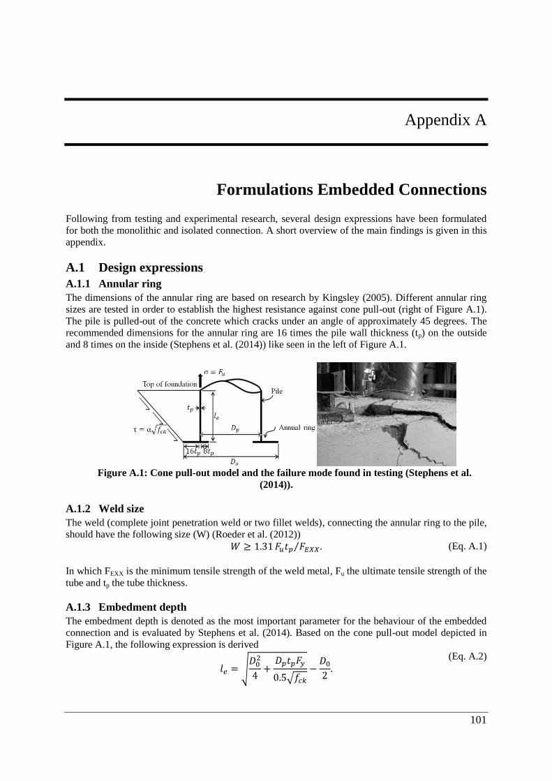
101
Appendix A
Appendix A Formulations Embedded Connections
Following from testing and experimental research, several design expressions have been formulated
for both the monolithic and isolated connection. A short overview of the main findings is given in this
appendix.
A.1 Design expressions
A.1.1 Annular ring
The dimensions of the annular ring are based on research by Kingsley (2005). Different annular ring
sizes are tested in order to establish the highest resistance against cone pull-out (right of Figure A.1).
The pile is pulled-out of the concrete which cracks under an angle of approximately 45 degrees. The
recommended dimensions for the annular ring are 16 times the pile wall thickness (tp) on the outside
and 8 times on the inside (Stephens et al. (2014)) like seen in the left of Figure A.1.
Figure A.1: Cone pull-out model and the failure mode found in testing (Stephens et al.
(2014)).
A.1.2 Weld size
The weld (complete joint penetration weld or two fillet welds), connecting the annular ring to the pile,
should have the following size (W) (Roeder et al. (2012))
𝑊 ≥ 1.31𝐹𝑢𝑡𝑝 𝐹𝐸𝑋𝑋⁄ . (Eq. A.1)
In which FEXX is the minimum tensile strength of the weld metal, Fu the ultimate tensile strength of the
tube and tp the tube thickness.
A.1.3 Embedment depth
The embedment depth is denoted as the most important parameter for the behaviour of the embedded
connection and is evaluated by Stephens et al. (2014). Based on the cone pull-out model depicted in
Figure A.1, the following expression is derived
𝑙𝑒 = √
𝐷02
4+𝐷𝑝𝑡𝑝𝐹𝑦
0.5√𝑓𝑐𝑘−𝐷02.
(Eq. A.2)
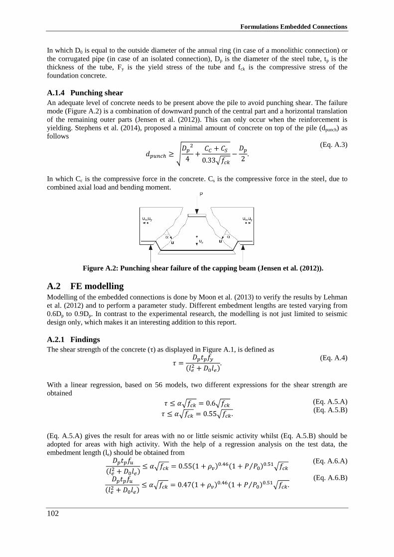
Formulations Embedded Connections
102
In which D0 is equal to the outside diameter of the annual ring (in case of a monolithic connection) or
the corrugated pipe (in case of an isolated connection), Dp is the diameter of the steel tube, tp is the
thickness of the tube, Fy is the yield stress of the tube and fck is the compressive stress of the
foundation concrete.
A.1.4 Punching shear
An adequate level of concrete needs to be present above the pile to avoid punching shear. The failure
mode (Figure A.2) is a combination of downward punch of the central part and a horizontal translation
of the remaining outer parts (Jensen et al. (2012)). This can only occur when the reinforcement is
yielding. Stephens et al. (2014), proposed a minimal amount of concrete on top of the pile (dpunch) as
follows
𝑑𝑝𝑢𝑛𝑐ℎ ≥ √𝐷𝑝
2
4+𝐶𝐶 + 𝐶𝑆
0.33√𝑓𝑐𝑘−𝐷𝑝
2.
(Eq. A.3)
In which Cc is the compressive force in the concrete. Cs is the compressive force in the steel, due to
combined axial load and bending moment.
Figure A.2: Punching shear failure of the capping beam (Jensen et al. (2012)).
A.2 FE modelling Modelling of the embedded connections is done by Moon et al. (2013) to verify the results by Lehman
et al. (2012) and to perform a parameter study. Different embedment lengths are tested varying from
0.6Dp to 0.9Dp. In contrast to the experimental research, the modelling is not just limited to seismic
design only, which makes it an interesting addition to this report.
A.2.1 Findings
The shear strength of the concrete (τ) as displayed in Figure A.1, is defined as
𝜏 =
𝐷𝑝𝑡𝑝𝑓𝑦
(𝑙𝑒2 + 𝐷0𝑙𝑒)
. (Eq. A.4)
With a linear regression, based on 56 models, two different expressions for the shear strength are
obtained
𝜏 ≤ 𝛼√𝑓𝑐𝑘 = 0.6√𝑓𝑐𝑘
𝜏 ≤ 𝛼√𝑓𝑐𝑘 = 0.55√𝑓𝑐𝑘.
(Eq. A.5.A)
(Eq. A.5.B)
(Eq. A.5.A) gives the result for areas with no or little seismic activity whilst (Eq. A.5.B) should be
adopted for areas with high activity. With the help of a regression analysis on the test data, the
embedment length (le) should be obtained from
𝐷𝑝𝑡𝑝𝑓𝑢
(𝑙𝑒2 + 𝐷0𝑙𝑒)
≤ 𝛼√𝑓𝑐𝑘 = 0.55(1 + 𝜌𝑣)0.46(1 + 𝑃 𝑃0⁄ )0.51√𝑓𝑐𝑘
𝐷𝑝𝑡𝑝𝑓𝑢(𝑙𝑒2 + 𝐷0𝑙𝑒)
≤ 𝛼√𝑓𝑐𝑘 = 0.47(1 + 𝜌𝑣)0.46(1 + 𝑃 𝑃0⁄ )0.51√𝑓𝑐𝑘.
(Eq. A.6.A)
(Eq. A.6.B)
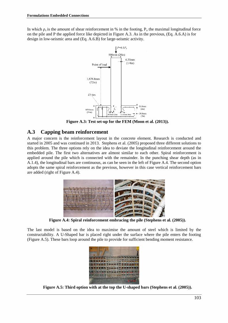
Formulations Embedded Connections
103
In which ρv is the amount of shear reinforcement in % in the footing, Po the maximal longitudinal force
on the pile and P the applied force like depicted in Figure A.3. As in the previous, (Eq. A.6.A) is for
design in low-seismic area and (Eq. A.6.B) for large-seismic activity.
Figure A.3: Test set-up for the FEM (Moon et al. (2013)).
A.3 Capping beam reinforcement A major concern is the reinforcement layout in the concrete element. Research is conducted and
started in 2005 and was continued in 2013. Stephens et al. (2005) proposed three different solutions to
this problem. The three options rely on the idea to deviate the longitudinal reinforcement around the
embedded pile. The first two alternatives are almost similar to each other. Spiral reinforcement is
applied around the pile which is connected with the remainder. In the punching shear depth (as in
A.1.4), the longitudinal bars are continuous, as can be seen in the left of Figure A.4. The second option
adopts the same spiral reinforcement as the previous, however in this case vertical reinforcement bars
are added (right of Figure A.4).
Figure A.4: Spiral reinforcement embracing the pile (Stephens et al. (2005)).
The last model is based on the idea to maximise the amount of steel which is limited by the
constructability. A U-Shaped bar is placed right under the surface where the pile enters the footing
(Figure A.5). These bars loop around the pile to provide for sufficient bending moment resistance.
Figure A.5: Third option with at the top the U-shaped bars (Stephens et al. (2005)).
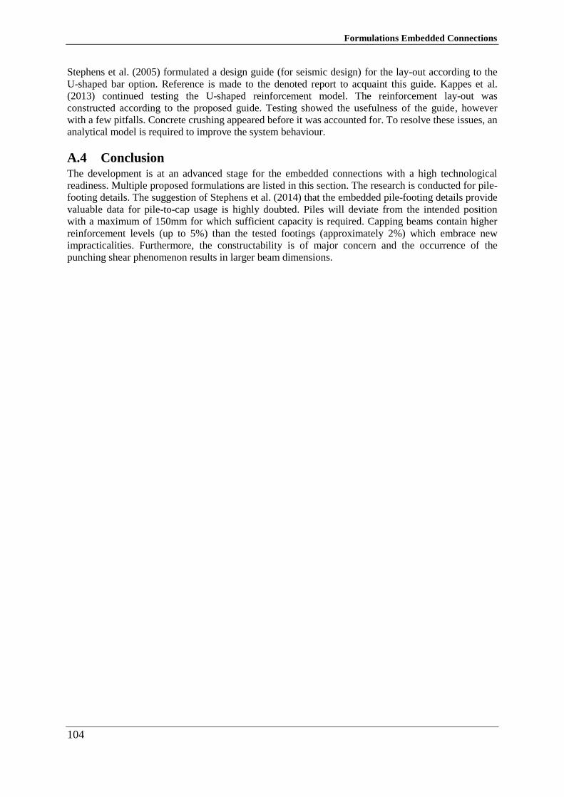
Formulations Embedded Connections
104
Stephens et al. (2005) formulated a design guide (for seismic design) for the lay-out according to the
U-shaped bar option. Reference is made to the denoted report to acquaint this guide. Kappes et al.
(2013) continued testing the U-shaped reinforcement model. The reinforcement lay-out was
constructed according to the proposed guide. Testing showed the usefulness of the guide, however
with a few pitfalls. Concrete crushing appeared before it was accounted for. To resolve these issues, an
analytical model is required to improve the system behaviour.
A.4 Conclusion The development is at an advanced stage for the embedded connections with a high technological
readiness. Multiple proposed formulations are listed in this section. The research is conducted for pile-
footing details. The suggestion of Stephens et al. (2014) that the embedded pile-footing details provide
valuable data for pile-to-cap usage is highly doubted. Piles will deviate from the intended position
with a maximum of 150mm for which sufficient capacity is required. Capping beams contain higher
reinforcement levels (up to 5%) than the tested footings (approximately 2%) which embrace new
impracticalities. Furthermore, the constructability is of major concern and the occurrence of the
punching shear phenomenon results in larger beam dimensions.
105
Appendix B
Appendix B Influential Aspects
Subsequent to the example in section 4.1, potential design influences are listed and subdivided. This
section gives an indication of the aspects involved and the decisions that are to be taken during the
design process. This information is obtained, based on available project data, interviews and literature.
B.1 Influences The composed list is given in Figure B.1. This figure illustrates the most important parameters which
are of influence. It is pointed out that during new projects, new aspects or conditions can arise which
are not included in the list.
Possible influencing aspects are clustered to keep a better overview of all the involved parameters.
Each group of aspects is elaborated in more detail in the following sections.
B.1.1 Construction aspects
The considered connection is adopted in several different construction types and situations. Even
within one construction, multiple solutions are adopted. Within a jetty, the piles may have
considerably shorter lengths near the shore compared to the ones positioned further away from shore.
Buckling lengths change and so will the capacity. This can be accommodated by filling the piles with
concrete for instance. To remain with the location, the outer piles need to resist most of the loads
induced by waves, berthing forces etc. This whilst the effect on the inner piles will remain limited.
Construction size and quantities determine the most economic lifting equipment. With small batches,
in-situ casting is preferred over prefabrication.
B.1.2 Function
It is already seen how the function can influence the design with the LNG jetty example (section 4.1).
If this same structure is a cargo jetty, it is necessary to deal with loads from handling equipment,
storage of containers, movements due to wind, berthing loads etc. One special consideration is made
regarding situations where fire ignition is possible. This results in totally different situations in
comparison to the earlier mentioned principles.
B.1.3 Loading
Loading conditions follow from the function of the structure, the type of construction and the local
conditions in which it is adopted. A distinction can be made between piles which need to transfer
axial- and shear force and piles which transfer bending moments as well.
B.1.4 Availability
The next issue is the availability of materials, labour and equipment. In some regions
experienced/classified labour is hard or impossible to get. In some extreme cases, labour from other
countries is flown in for specific jobs. The same applies to equipment. The design should be adapted
to the available cranes, vessels etc.
Influential Aspects
106
B.1.5 Possible lifting weight
Following from the accessibility of the site, the availability of equipment, the local conditions and the
construction size, the most cost effective equipment is chosen. The magnitude of the possible lifting
capacity will determine the installation method of the piles and therefore the capacity, the construction
method of the concrete element and thus the connection design.
B.1.6 Local conditions
Local conditions include wave-, water-, wind-, scour-, soil-, marine and climate conditions. Wave
height sets the construction height, which subsequently influences the pile lengths. Water conditions
like tidal data are already discussed with the jetty example. Climate conditions change material
behaviour, the curing conditions for the concrete or ice loads might be present. Local soil conditions
affect the construction- and installation method of the pipe piles. In soft soil, the herniation point is
low down which results in long buckling lengths of the pipe piles, hard soil conditions result in a high
herniation point.
B.1.7 Capacity and installation method piles
The required capacity is defined by the loading conditions following from the function and the type of
construction. The possible capacity is subsequently determined by the local soil conditions, which
influence the bearing capacity and the buckling capacity. External loading on the piles is induced by
wave, wind and ice actions which is dependent on the local conditions. Furthermore, marine life might
have an impact on the installation method, since it might affect animal behaviour during some time of
the year due to noise and vibrations.
B.1.8 Practical experience
Common practice within an engineering department plays an important role in design. When a
previous adopted alternative works properly, it is likely that this alternative is reused in new projects.
Switching from alternative means investing in obtaining new knowledge, new design rules and
laboratory testing.
B.2 Decisions To get a grip on the design issue, the matter is subdivided into several decisions prior to the decision
for the connection. These decisions follow from the influence groups from the previous section.
Design decisions include the production method of the capping beam, the installation method of the
piles, construction speed etc. To illustrate the basic design idea, the scheme in Figure B.2 is compiled.
The process starts at the basic principles which are known, namely local conditions and the type of
structure. Subsequently, more detailed data is gathered concerning soil- and water properties,
availability of equipment and materials etc. This contextual information is used for establishing the
proper hoist equipment, the design loads and the required location-bound information.
The scheme is composed as follows: the bold printed texts are the groups as defined in section B.1.
The round boxes indicate that properties need to be determined. A normal line stands for a link and an
arrow for a design decision. The small boxes are the possible outcomes. When for instance the lifting
weights are known, a decision can be made for the production method of the capping beam. This can
be an in-situ solution, prefab or box option.
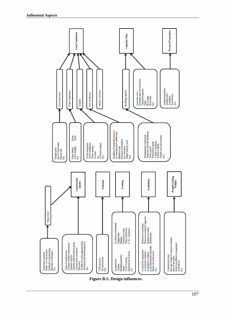
Influential Aspects
107
Figure B.1: Design influences.
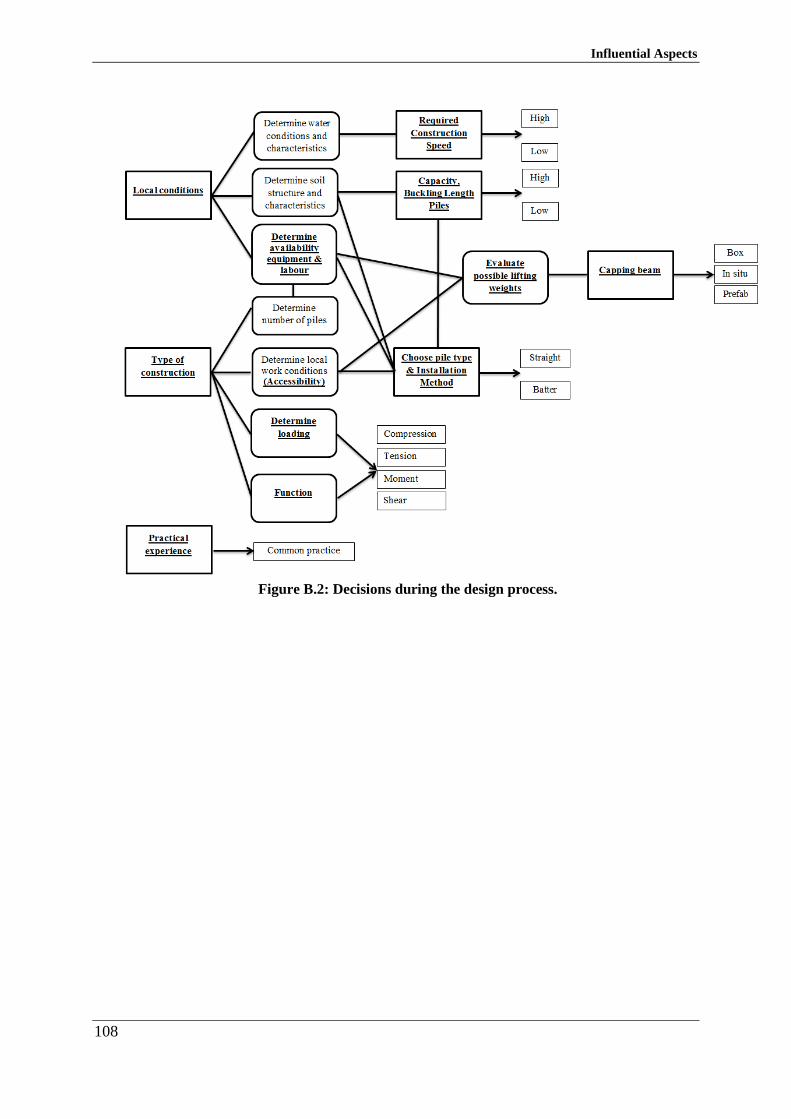
Influential Aspects
108
Figure B.2: Decisions during the design process.
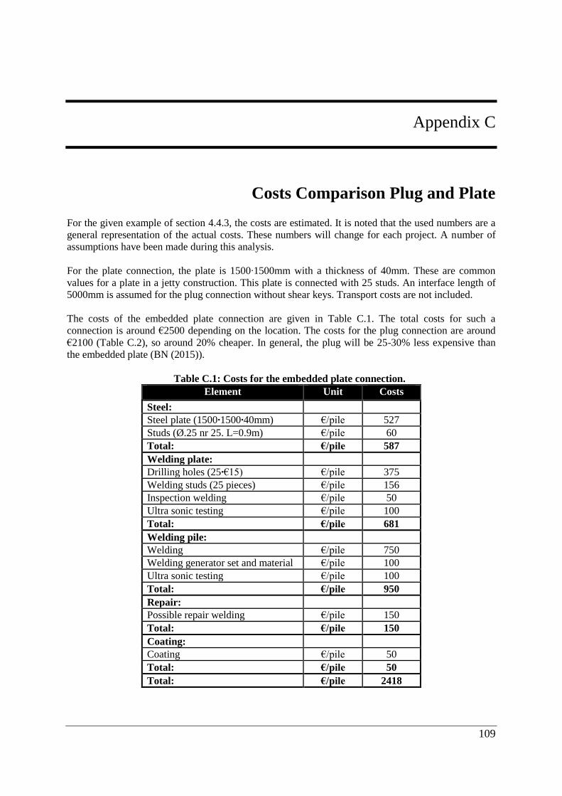
109
Appendix C
Appendix C Costs Comparison Plug and Plate
For the given example of section 4.4.3, the costs are estimated. It is noted that the used numbers are a
general representation of the actual costs. These numbers will change for each project. A number of
assumptions have been made during this analysis.
For the plate connection, the plate is 1500∙1500mm with a thickness of 40mm. These are common
values for a plate in a jetty construction. This plate is connected with 25 studs. An interface length of
5000mm is assumed for the plug connection without shear keys. Transport costs are not included.
The costs of the embedded plate connection are given in Table C.1. The total costs for such a
connection is around €2500 depending on the location. The costs for the plug connection are around
€2100 (Table C.2), so around 20% cheaper. In general, the plug will be 25-30% less expensive than
the embedded plate (BN (2015)).
Table C.1: Costs for the embedded plate connection.
Element Unit Costs
Steel:
Steel plate (1500∙1500∙40mm) €/pile 527
Studs (Ø.25 nr 25. L=0.9m) €/pile 60
Total: €/pile 587
Welding plate:
Drilling holes (25∙€15) €/pile 375
Welding studs (25 pieces) €/pile 156
Inspection welding €/pile 50
Ultra sonic testing €/pile 100
Total: €/pile 681
Welding pile:
Welding €/pile 750
Welding generator set and material €/pile 100
Ultra sonic testing €/pile 100
Total: €/pile 950
Repair:
Possible repair welding €/pile 150
Total: €/pile 150
Coating:
Coating €/pile 50
Total: €/pile 50
Total: €/pile 2418
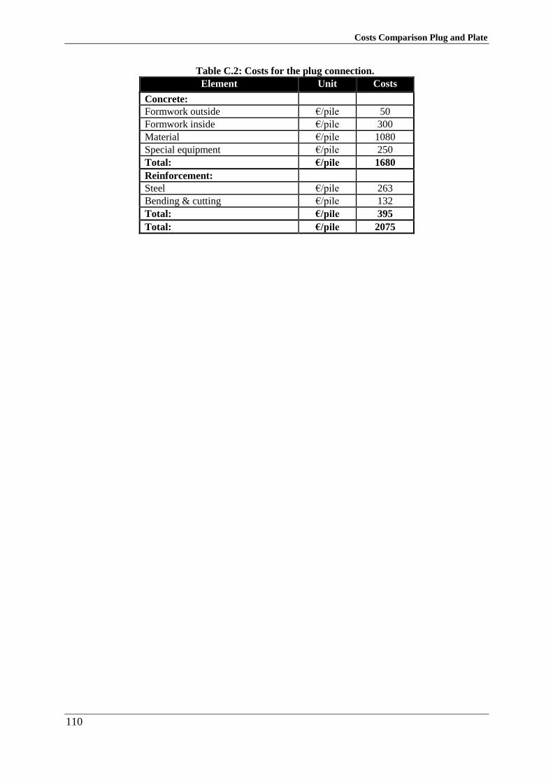
Costs Comparison Plug and Plate
110
Table C.2: Costs for the plug connection.
Element Unit Costs
Concrete:
Formwork outside €/pile 50
Formwork inside €/pile 300
Material €/pile 1080
Special equipment €/pile 250
Total: €/pile 1680
Reinforcement:
Steel €/pile 263
Bending & cutting €/pile 132
Total: €/pile 395
Total: €/pile 2075
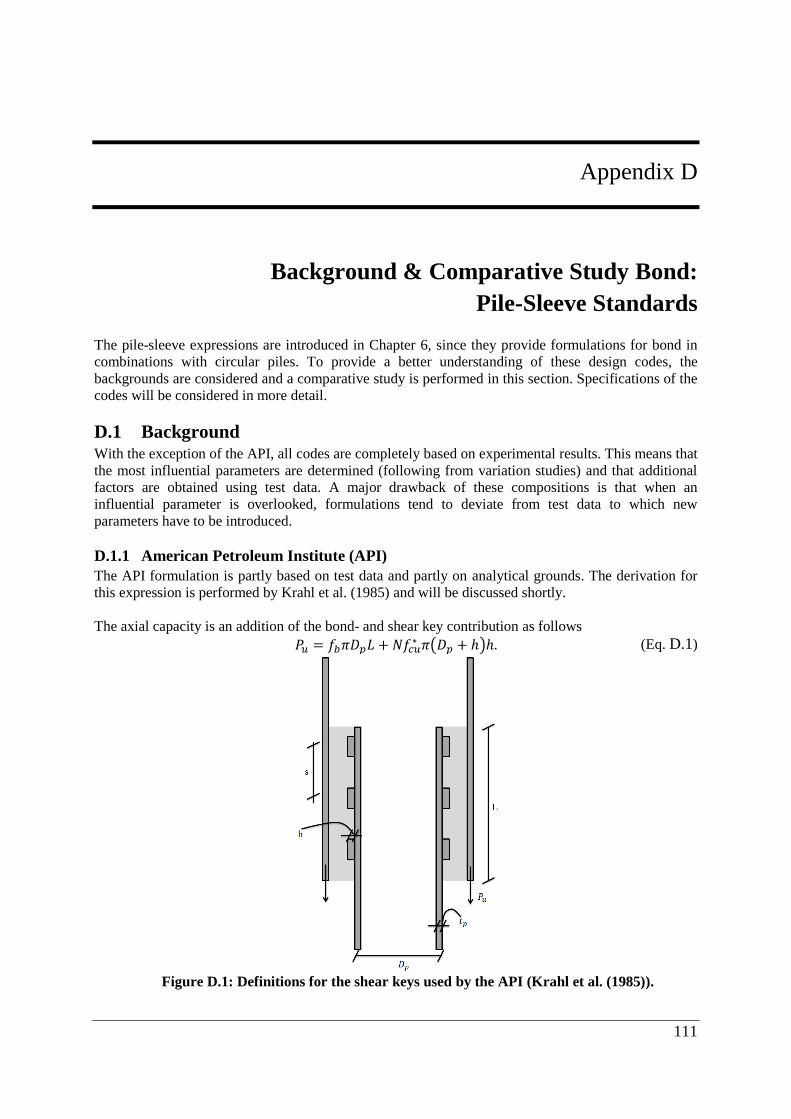
111
Appendix D
Appendix D Background & Comparative Study Bond:
Pile-Sleeve Standards
The pile-sleeve expressions are introduced in Chapter 6, since they provide formulations for bond in
combinations with circular piles. To provide a better understanding of these design codes, the
backgrounds are considered and a comparative study is performed in this section. Specifications of the
codes will be considered in more detail.
D.1 Background With the exception of the API, all codes are completely based on experimental results. This means that
the most influential parameters are determined (following from variation studies) and that additional
factors are obtained using test data. A major drawback of these compositions is that when an
influential parameter is overlooked, formulations tend to deviate from test data to which new
parameters have to be introduced.
D.1.1 American Petroleum Institute (API)
The API formulation is partly based on test data and partly on analytical grounds. The derivation for
this expression is performed by Krahl et al. (1985) and will be discussed shortly.
The axial capacity is an addition of the bond- and shear key contribution as follows
𝑃𝑢 = 𝑓𝑏𝜋𝐷𝑝𝐿 + 𝑁𝑓𝑐𝑢∗ 𝜋(𝐷𝑝 + ℎ)ℎ. (Eq. D.1)
Figure D.1: Definitions for the shear keys used by the API (Krahl et al. (1985)).
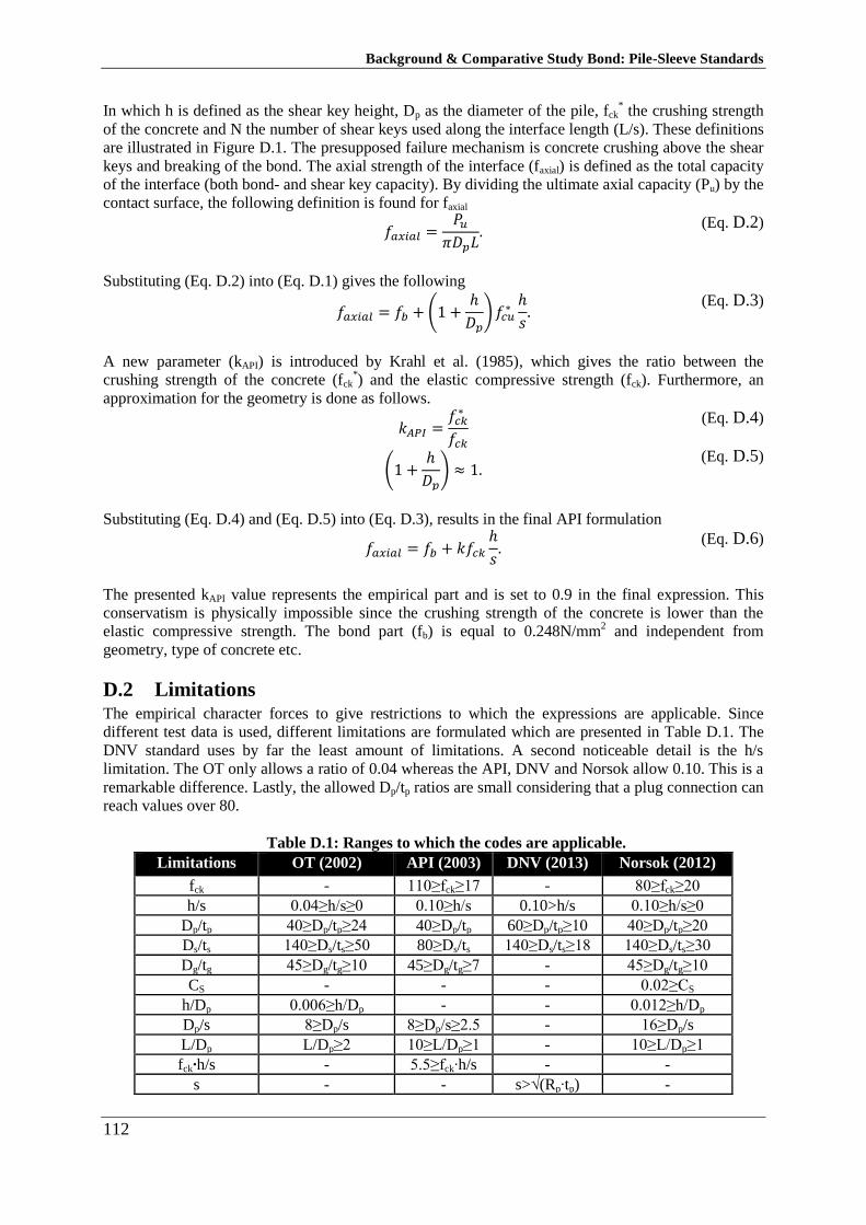
Background & Comparative Study Bond: Pile-Sleeve Standards
112
In which h is defined as the shear key height, Dp as the diameter of the pile, fck* the crushing strength
of the concrete and N the number of shear keys used along the interface length (L/s). These definitions
are illustrated in Figure D.1. The presupposed failure mechanism is concrete crushing above the shear
keys and breaking of the bond. The axial strength of the interface (faxial) is defined as the total capacity
of the interface (both bond- and shear key capacity). By dividing the ultimate axial capacity (Pu) by the
contact surface, the following definition is found for faxial
𝑓𝑎𝑥𝑖𝑎𝑙 =
𝑃𝑢𝜋𝐷𝑝𝐿
. (Eq. D.2)
Substituting (Eq. D.2) into (Eq. D.1) gives the following
𝑓𝑎𝑥𝑖𝑎𝑙 = 𝑓𝑏 + (1 +
ℎ
𝐷𝑝)𝑓𝑐𝑢
∗ℎ
𝑠.
(Eq. D.3)
A new parameter (kAPI) is introduced by Krahl et al. (1985), which gives the ratio between the
crushing strength of the concrete (fck*) and the elastic compressive strength (fck). Furthermore, an
approximation for the geometry is done as follows.
𝑘𝐴𝑃𝐼 =
𝑓𝑐𝑘∗
𝑓𝑐𝑘
(1 +ℎ
𝐷𝑝) ≈ 1.
(Eq. D.4)
(Eq. D.5)
Substituting (Eq. D.4) and (Eq. D.5) into (Eq. D.3), results in the final API formulation
𝑓𝑎𝑥𝑖𝑎𝑙 = 𝑓𝑏 + 𝑘𝑓𝑐𝑘
ℎ
𝑠.
(Eq. D.6)
The presented kAPI value represents the empirical part and is set to 0.9 in the final expression. This
conservatism is physically impossible since the crushing strength of the concrete is lower than the
elastic compressive strength. The bond part (fb) is equal to 0.248N/mm2 and independent from
geometry, type of concrete etc.
D.2 Limitations The empirical character forces to give restrictions to which the expressions are applicable. Since
different test data is used, different limitations are formulated which are presented in Table D.1. The
DNV standard uses by far the least amount of limitations. A second noticeable detail is the h/s
limitation. The OT only allows a ratio of 0.04 whereas the API, DNV and Norsok allow 0.10. This is a
remarkable difference. Lastly, the allowed Dp/tp ratios are small considering that a plug connection can
reach values over 80.
Table D.1: Ranges to which the codes are applicable.
Limitations OT (2002) API (2003) DNV (2013) Norsok (2012)
fck - 110≥fck≥17 - 80≥fck≥20
h/s 0.04≥h/s≥0 0.10≥h/s 0.10>h/s 0.10≥h/s≥0
Dp/tp 40≥Dp/tp≥24 40≥Dp/tp 60≥Dp/tp≥10 40≥Dp/tp≥20
Ds/ts 140≥Ds/ts≥50 80≥Ds/ts 140≥Ds/ts≥18 140≥Ds/ts≥30
Dg/tg 45≥Dg/tg≥10 45≥Dg/tg≥7 - 45≥Dg/tg≥10
CS - - - 0.02≥CS
h/Dp 0.006≥h/Dp - - 0.012≥h/Dp
Dp/s 8≥Dp/s 8≥Dp/s≥2.5 - 16≥Dp/s
L/Dp L/Dp≥2 10≥L/Dp≥1 - 10≥L/Dp≥1
fck∙h/s - 5.5≥fck∙h/s - -
s - - s>√(Rp∙tp) -
Background & Comparative Study Bond: Pile-Sleeve Standards
113
D.3 Design factors In each standard, different design factors are assigned. Design factors include safety-, material- and/or
load factors. The Offshore Technology (OT) uses a design factor of 6.0 during normal conditions
which is lowered to 4.5 in extreme conditions. This includes a load factor of 1.5, a material factor of
1.5 and a behaviour factor accounting for grouting conditions, cyclic loading effects, incomplete
grouting and differences in compressive strength between on- and offshore (Billington et al. (1980)).
DNV (2010) and Norsok both apply material factors which are respectively 3.0 and 2.0 during normal
operating conditions. DNV (2013) prescribes a material factor around 1.5 till 1.75 depending on the
thickness of the grout layer. This values can only be used when small grout thicknesses are adopted
which does not hold for the plug connections. Therefore, the material factor of 3.0 is applied which
counts for offshore grouting operations. Lastly, the American design code applies a resistance factor
for the axial load transfer stress equal to 0.9. The API factor seems low in relation to the other
standards, however the kAPI value which is adopted in their formulation is chosen very conservatively.
Appropriate safety is arranged in this manner instead of applying higher factors.
D.4 Comparison between pile-sleeve codes Comparing formulations of all four pile-sleeve systems result in the following findings. Agreements
between codes are:
Three formulations are completely empirical meaning they are fitted to test results,
All four codes add up the bond- and the shear key part (implying the same load deflection
curves),
The shear key transfer strength is dependent on the ratio of the outstand divided by the spacing
h/s, see Figure D.1,
The interface strength of the connection is a function of the concrete compressive strength,
OT and Norsok apply the same stiffness parameter. DNV uses a similar which gives slightly
different results.
Differences between codes are:
The API uses one single independent value for bond whereas the OT and Norsok involve a
stiffness factor (based on Billington’s findings),
Norsok incorporates surface irregularities,
Norsok includes a flexibility factor.
Further remarks which can be made are:
The API does not involve the geometry of the connecting elements. This seems unreasonable
since experimental results show lowering of strength with increasing diameters (also in the
pile-sleeve format),
The stiffness parameters in the OT, DNV and Norsok account for the Dp/tp ratio of the pile, the
sleeve and the grout. However, like noted in Table D.1, no limitation for the maximum pile
thickness and diameter are given. This means when the thickness is increased linearly with the
diameter of the pile, the diameter over thickness ratio keeps constant and the capacity remains
constant. This is contrary to the conclusions from Chapter 6 in which shrinkage is depicted as
one of the major influences,
Again, it is pointed out that the plug- and the pile-sleeve are two different systems. Mutual
differences are present.
D.5 Comparative study bond From literature (Chapter 6), a number of parameters show large influences on the bond capacity in
plug connections. To check whether the formulations follow these trends and show corresponding
results, a parameter study is performed. All expressions for the bond capacity are included in this
analysis. The design example from section 6.5.4 is used as guidance during this analysis unless stated
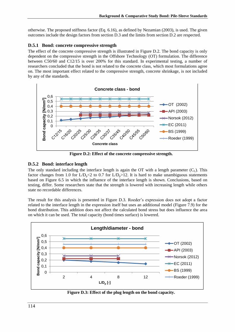
Background & Comparative Study Bond: Pile-Sleeve Standards
114
otherwise. The proposed stiffness factor (Eq. 6.16), as defined by Nezamian (2003), is used. The given
outcomes include the design factors from section D.3 and the limits from section D.2 are respected.
D.5.1 Bond: concrete compressive strength
The effect of the concrete compressive strength is illustrated in Figure D.2. The bond capacity is only
dependent on the compressive strength in the Offshore Technology (OT) formulation. The difference
between C50/60 and C12/15 is over 200% for this standard. In experimental testing, a number of
researchers concluded that the bond is not related to the concrete class, which most formulations agree
on. The most important effect related to the compressive strength, concrete shrinkage, is not included
by any of the standards.
Figure D.2: Effect of the concrete compressive strength.
D.5.2 Bond: interface length
The only standard including the interface length is again the OT with a length parameter (CL). This
factor changes from 1.0 for L/Dp<2 to 0.7 for L/Dp>12. It is hard to make unambiguous statements
based on Figure 6.5 in which the influence of the interface length is shown. Conclusions, based on
testing, differ. Some researchers state that the strength is lowered with increasing length while others
state no recordable differences.
The result for this analysis is presented in Figure D.3. Roeder’s expression does not adopt a factor
related to the interface length in the expression itself but uses an additional model (Figure 7.9) for the
bond distribution. This addition does not affect the calculated bond stress but does influence the area
on which it can be used. The total capacity (bond times surface) is lowered.
Figure D.3: Effect of the plug length on the bond capacity.
0
0,1
0,2
0,3
0,4
0,5
0,6
Bo
nd
cap
acit
y [
N/m
m2]
Concrete class
Concrete class - bond
OT (2002)
API (2003)
Norsok (2012)
EC (2011)
BS (1999)
Roeder (1999)
0
0,1
0,2
0,3
0,4
0,5
0,6
2 4 8 12
Bo
nd
ca
pa
cit
y [
N/m
m2]
L/Dp [-]
Length/diameter - bond
OT (2002)
API (2003)
Norsok (2012)
EC (2011)
BS (1999)
Roeder (1999)
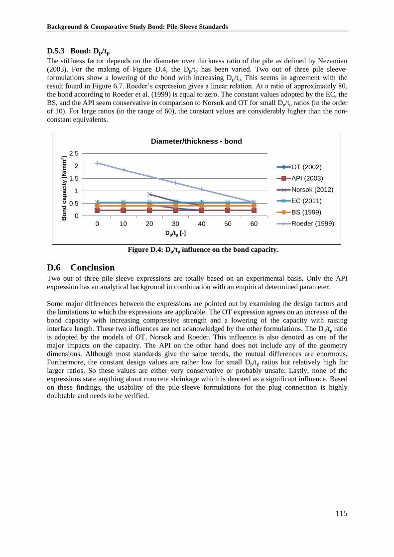
Background & Comparative Study Bond: Pile-Sleeve Standards
115
D.5.3 Bond: Dp/tp
The stiffness factor depends on the diameter over thickness ratio of the pile as defined by Nezamian
(2003). For the making of Figure D.4, the Dp/tp has been varied. Two out of three pile sleeve-
formulations show a lowering of the bond with increasing Dp/tp. This seems in agreement with the
result found in Figure 6.7. Roeder’s expression gives a linear relation. At a ratio of approximately 80,
the bond according to Roeder et al. (1999) is equal to zero. The constant values adopted by the EC, the
BS, and the API seem conservative in comparison to Norsok and OT for small Dp/tp ratios (in the order
of 10). For large ratios (in the range of 60), the constant values are considerably higher than the non-
constant equivalents.
Figure D.4: Dp/tp influence on the bond capacity.
D.6 Conclusion Two out of three pile sleeve expressions are totally based on an experimental basis. Only the API
expression has an analytical background in combination with an empirical determined parameter.
Some major differences between the expressions are pointed out by examining the design factors and
the limitations to which the expressions are applicable. The OT expression agrees on an increase of the
bond capacity with increasing compressive strength and a lowering of the capacity with raising
interface length. These two influences are not acknowledged by the other formulations. The Dp/tp ratio
is adopted by the models of OT, Norsok and Roeder. This influence is also denoted as one of the
major impacts on the capacity. The API on the other hand does not include any of the geometry
dimensions. Although most standards give the same trends, the mutual differences are enormous.
Furthermore, the constant design values are rather low for small Dp/tp ratios but relatively high for
larger ratios. So these values are either very conservative or probably unsafe. Lastly, none of the
expressions state anything about concrete shrinkage which is denoted as a significant influence. Based
on these findings, the usability of the pile-sleeve formulations for the plug connection is highly
doubtable and needs to be verified.
0
0,5
1
1,5
2
2,5
0 10 20 30 40 50 60
Bo
nd
ca
pa
cit
y [
N/m
m2]
Dp/tp [-]
Diameter/thickness - bond
OT (2002)
API (2003)
Norsok (2012)
EC (2011)
BS (1999)
Roeder (1999)
Background & Comparative Study Bond: Pile-Sleeve Standards
116
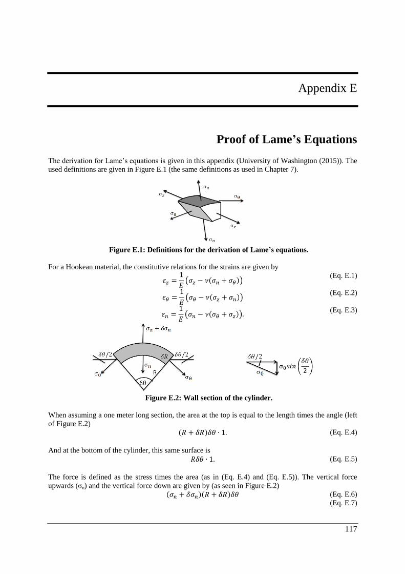
117
Appendix E
Appendix E Proof of Lame’s Equations
The derivation for Lame’s equations is given in this appendix (University of Washington (2015)). The
used definitions are given in Figure E.1 (the same definitions as used in Chapter 7).
Figure E.1: Definitions for the derivation of Lame’s equations.
For a Hookean material, the constitutive relations for the strains are given by
휀𝑧 =
1
𝐸(𝜎𝑧 − 𝜈(𝜎𝑛 + 𝜎𝜃))
휀𝜃 =1
𝐸(𝜎𝜃 − 𝜈(𝜎𝑧 + 𝜎𝑛))
휀𝑛 =1
𝐸(𝜎𝑛 − 𝜈(𝜎𝜃 + 𝜎𝑧)).
(Eq. E.1)
(Eq. E.2)
(Eq. E.3)
Figure E.2: Wall section of the cylinder.
When assuming a one meter long section, the area at the top is equal to the length times the angle (left
of Figure E.2)
(𝑅 + 𝛿𝑅)𝛿𝜃 ∙ 1. (Eq. E.4)
And at the bottom of the cylinder, this same surface is
𝑅𝛿𝜃 ∙ 1. (Eq. E.5)
The force is defined as the stress times the area (as in (Eq. E.4) and (Eq. E.5)). The vertical force
upwards (σn) and the vertical force down are given by (as seen in Figure E.2)
(𝜎𝑛 + 𝛿𝜎𝑛)(𝑅 + 𝛿𝑅)𝛿𝜃 (Eq. E.6)
(Eq. E.7)
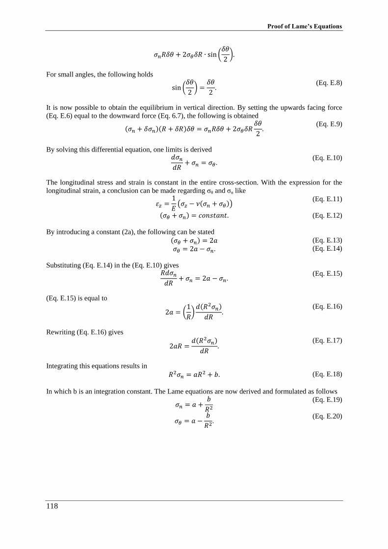
Proof of Lame’s Equations
118
𝜎𝑛𝑅𝛿𝜃 + 2𝜎𝜃𝛿𝑅 ∙ sin (𝛿𝜃
2).
For small angles, the following holds
sin (
𝛿𝜃
2) =
𝛿𝜃
2.
(Eq. E.8)
It is now possible to obtain the equilibrium in vertical direction. By setting the upwards facing force
(Eq. E.6) equal to the downward force (Eq. 6.7), the following is obtained
(𝜎𝑛 + 𝛿𝜎𝑛)(𝑅 + 𝛿𝑅)𝛿𝜃 = 𝜎𝑛𝑅𝛿𝜃 + 2𝜎𝜃𝛿𝑅
𝛿𝜃
2.
(Eq. E.9)
By solving this differential equation, one limits is derived
𝑑𝜎𝑛𝑑𝑅
+ 𝜎𝑛 = 𝜎𝜃. (Eq. E.10)
The longitudinal stress and strain is constant in the entire cross-section. With the expression for the
longitudinal strain, a conclusion can be made regarding σθ and σn like
휀𝑧 =
1
𝐸(𝜎𝑧 − 𝜈(𝜎𝑛 + 𝜎𝜃))
(𝜎𝜃 + 𝜎𝑛) = 𝑐𝑜𝑛𝑠𝑡𝑎𝑛𝑡.
(Eq. E.11)
(Eq. E.12)
By introducing a constant (2a), the following can be stated
(𝜎𝜃 + 𝜎𝑛) = 2𝑎
𝜎𝜃 = 2𝑎 − 𝜎𝑛. (Eq. E.13)
(Eq. E.14)
Substituting (Eq. E.14) in the (Eq. E.10) gives
𝑅𝑑𝜎𝑛𝑑𝑅
+ 𝜎𝑛 = 2𝑎 − 𝜎𝑛. (Eq. E.15)
(Eq. E.15) is equal to
2𝑎 = (
1
𝑅)𝑑(𝑅2𝜎𝑛)
𝑑𝑅.
(Eq. E.16)
Rewriting (Eq. E.16) gives
2𝑎𝑅 =
𝑑(𝑅2𝜎𝑛)
𝑑𝑅.
(Eq. E.17)
Integrating this equations results in
𝑅2𝜎𝑛 = 𝑎𝑅2 + 𝑏. (Eq. E.18)
In which b is an integration constant. The Lame equations are now derived and formulated as follows
𝜎𝑛 = 𝑎 +
𝑏
𝑅2
𝜎𝜃 = 𝑎 −𝑏
𝑅2.
(Eq. E.19)
(Eq. E.20)
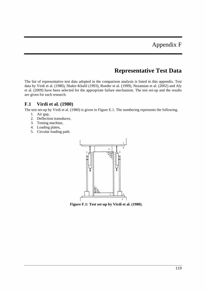
119
Appendix F
Appendix F Representative Test Data
The list of representative test data adopted in the comparison analysis is listed in this appendix. Test
data by Virdi et al. (1980), Shakir-Khalil (1993), Roeder et al. (1999), Nezamian et al. (2002) and Aly
et al. (2009) have been selected for the appropriate failure mechanism. The test set-up and the results
are given for each research.
F.1 Virdi et al. (1980) The test set-up by Virdi et al. (1980) is given in Figure E.1. The numbering represents the following.
1. Air gap,
2. Deflection transduces,
3. Testing machine,
4. Loading plates,
5. Circular loading path.
Figure F.1: Test set-up by Virdi et al. (1980).
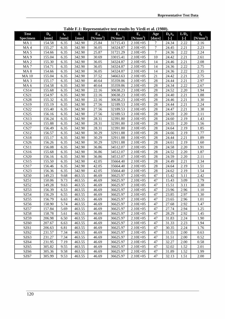
Representative Test Data
120
Table F.1: Representative test results by Virdi et al. (1980).
Test
Specimen
Dp
[mm]
tp
[mm]
L
[mm]
Fck
[N/mm2]
Ec
[N/mm2]
Es
[N/mm2]
Age
[days]
Dp/tp
[-]
L/Dp
[-]
fb
[N/mm2]
MA 1 154.58 6.35 342.90 25.84 31715.43 2.10E+05 7 24.34 2.22 2.16
MA 4 155.27 6.35 342.90 36.05 34324.87 2.10E+05 7 24.45 2.21 2.23
MA 5 154.66 6.35 342.90 25.87 31721.29 2.10E+05 7 24.36 2.22 2.24
MA 9 155.04 6.35 342.90 30.69 33015.41 2.10E+05 10 24.42 2.21 2.61
MA 2 155.30 6.35 342.90 36.05 34324.87 2.10E+05 14 24.46 2.21 2.08
MA 7 154.71 6.35 342.90 36.05 34324.87 2.10E+05 14 24.36 2.22 2.75
MA 8 154.66 6.35 342.90 36.05 34324.87 2.10E+05 14 24.36 2.22 2.35
MA 10 155.04 6.35 342.90 37.52 34663.63 2.10E+05 21 24.42 2.21 2.75
MA 3 155.17 6.35 342.90 40.64 35359.86 2.10E+05 28 24.44 2.21 2.97
MA 6 154.58 6.35 342.90 40.64 35359.86 2.10E+05 28 24.34 2.22 2.67
CS14 155.68 6.35 342.90 22.16 30638.23 2.10E+05 28 24.52 2.20 1.94
CS21 154.97 6.35 342.90 22.16 30638.23 2.10E+05 28 24.40 2.21 1.88
CS28 155.32 6.35 342.90 22.16 30638.23 2.10E+05 28 24.46 2.21 1.30
CS19 155.19 6.35 342.90 27.56 32189.53 2.10E+05 28 24.44 2.21 2.24
CS22 155.40 6.35 342.90 27.56 32189.53 2.10E+05 28 24.47 2.21 1.38
CS25 156.16 6.35 342.90 27.56 32189.53 2.10E+05 28 24.59 2.20 2.11
CS13 156.24 6.35 342.90 28.31 32391.80 2.10E+05 28 24.60 2.19 1.43
CS24 155.88 6.35 342.90 28.31 32391.80 2.10E+05 28 24.55 2.20 1.56
CS27 156.49 6.35 342.90 28.31 32391.80 2.10E+05 28 24.64 2.19 1.85
CS12 156.57 6.35 342.90 30.29 32911.88 2.10E+05 28 24.66 2.19 1.77
CS18 155.17 6.35 342.90 30.29 32911.88 2.10E+05 28 24.44 2.21 1.89
CS26 156.26 6.35 342.90 30.29 32911.88 2.10E+05 28 24.61 2.19 1.60
CS11 156.08 6.35 342.90 36.86 34512.07 2.10E+05 28 24.58 2.20 1.91
CS16 155.68 6.35 342.90 36.86 34512.07 2.10E+05 28 24.52 2.20 1.87
CS20 156.16 6.35 342.90 36.86 34512.07 2.10E+05 28 24.59 2.20 2.11
CS15 155.50 6.35 342.90 42.05 35664.40 2.10E+05 28 24.49 2.21 2.34
CS17 156.46 6.35 342.90 42.05 35664.40 2.10E+05 28 24.64 2.19 1.51
CS23 156.36 6.35 342.90 42.05 35664.40 2.10E+05 28 24.62 2.19 1.54
SZ50 149.23 9.68 463.55 46.69 36625.97 2.10E+05 47 15.42 3.11 2.42
SZ51 150.06 9.73 463.55 46.69 36625.97 2.10E+05 47 15.43 3.09 1.79
SZ52 149.28 9.63 463.55 46.69 36625.97 2.10E+05 47 15.51 3.11 2.38
SZ53 156.39 6.53 463.55 46.69 36625.97 2.10E+05 47 23.96 2.96 1.10
SZ54 156.29 6.55 463.55 46.69 36625.97 2.10E+05 47 23.85 2.97 1.30
SZ55 156.79 6.63 463.55 46.69 36625.97 2.10E+05 47 23.65 2.96 1.01
SZ56 158.90 5.74 463.55 46.69 36625.97 2.10E+05 47 27.68 2.92 1.47
SZ57 157.84 5.69 463.55 46.69 36625.97 2.10E+05 47 27.74 2.94 1.25
SZ58 158.78 5.61 463.55 46.69 36625.97 2.10E+05 47 28.29 2.92 1.45
SZ59 206.98 6.50 463.55 46.69 36625.97 2.10E+05 47 31.83 2.24 1.90
SZ60 207.67 6.63 463.55 46.69 36625.97 2.10E+05 47 31.33 2.23 1.94
SZ61 206.63 6.81 463.55 46.69 36625.97 2.10E+05 47 30.35 2.24 1.76
SZ62 231.57 7.34 463.55 46.69 36625.97 2.10E+05 47 31.55 2.00 0.63
SZ63 231.27 7.34 463.55 46.69 36625.97 2.10E+05 47 31.51 2.00 0.52
SZ64 231.95 7.19 463.55 46.69 36625.97 2.10E+05 47 32.27 2.00 0.58
SZ65 305.82 9.55 463.55 46.69 36625.97 2.10E+05 47 32.02 1.52 2.01
SZ66 305.36 9.58 463.55 46.69 36625.97 2.10E+05 47 31.89 1.52 1.99
SZ67 305.99 9.53 463.55 46.69 36625.97 2.10E+05 47 32.13 1.51 2.00
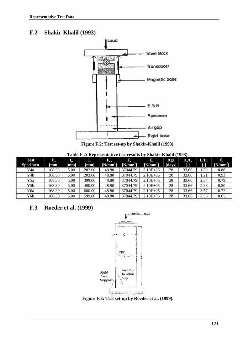
Representative Test Data
121
F.2 Shakir-Khalil (1993)
Figure F.2: Test set-up by Shakir-Khalil (1993).
Table F.2: Representative test results by Shakir-Khalil (1993).
Test
Specimen
Dp
[mm]
tp
[mm]
L
[mm]
Fck
[N/mm2]
Ec
[N/mm2]
Es
[N/mm2]
Age
[days]
Dp/tp
[-]
L/Dp
[-]
fb
[N/mm2]
Y4a 168.30 5.00 202.00 48.80 37044.79 2.10E+05 28 33.66 1.20 0.88
Y4b 168.30 5.00 203.00 48.80 37044.79 2.10E+05 28 33.66 1.21 0.93
Y5a 168.30 5.00 399.00 48.80 37044.79 2.10E+05 28 33.66 2.37 0.79
Y5b 168.30 5.00 400.00 48.80 37044.79 2.10E+05 28 33.66 2.38 0.80
Y6a 168.30 5.00 600.00 48.80 37044.79 2.10E+05 28 33.66 3.57 0.72
Y6b 168.30 5.00 599.00 48.80 37044.79 2.10E+05 28 33.66 3.56 0.65
F.3 Roeder et al. (1999)
Figure F.3: Test set-up by Roeder et al. (1999).
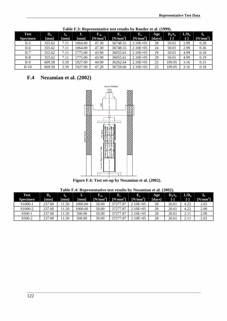
Representative Test Data
122
Table F.3: Representative test results by Roeder et al. (1999).
Test
Specimen
Dp
[mm]
tp
[mm]
L
[mm]
Fck
[N/mm2]
Ec
[N/mm2]
Es
[N/mm2]
Age
[days]
Dp/tp
[-]
L/Dp
[-]
fb
[N/mm2]
II-5 355.62 7.11 1064.00 47.30 36748.55 2.10E+05 28 50.01 2.99 0.28
II-6 355.62 7.11 1064.00 47.30 36748.55 2.10E+05 24 50.01 2.99 0.36
II-7 355.62 7.11 1775.00 43.90 36055.61 2.10E+05 29 50.01 4.99 0.18
II-8 355.62 7.11 1775.00 43.90 36055.61 2.10E+05 29 50.01 4.99 0.19
II-9 609.58 5.59 1927.00 44.90 36262.64 2.10E+05 25 109.05 3.16 0.15
II-10 609.58 5.59 1927.00 47.20 36728.60 2.10E+05 25 109.05 3.16 0.18
F.4 Nezamian et al. (2002)
Figure F.4: Test set-up by Nezamian et al. (2002).
Table F.4: Representative test results by Nezamian et al. (2002).
Test
Specimen
Dp
[mm]
tp
[mm]
L
[mm]
Fck
[N/mm2]
Ec
[N/mm2]
Es
[N/mm2]
Age
[days]
Dp/tp
[-]
L/Dp
[-]
fb
[N/mm2]
S1000-1 237.00 11.50 1000.00 50.00 37277.87 2.10E+05 28 20.61 4.22 2.02
S1000-2 237.00 11.50 1000.00 50.00 37277.87 2.10E+05 28 20.61 4.22 2.00
S500-1 237.00 11.50 500.00 50.00 37277.87 2.10E+05 28 20.61 2.11 2.06
S500-2 237.00 11.50 500.00 50.00 37277.87 2.10E+05 28 20.61 2.11 2.02
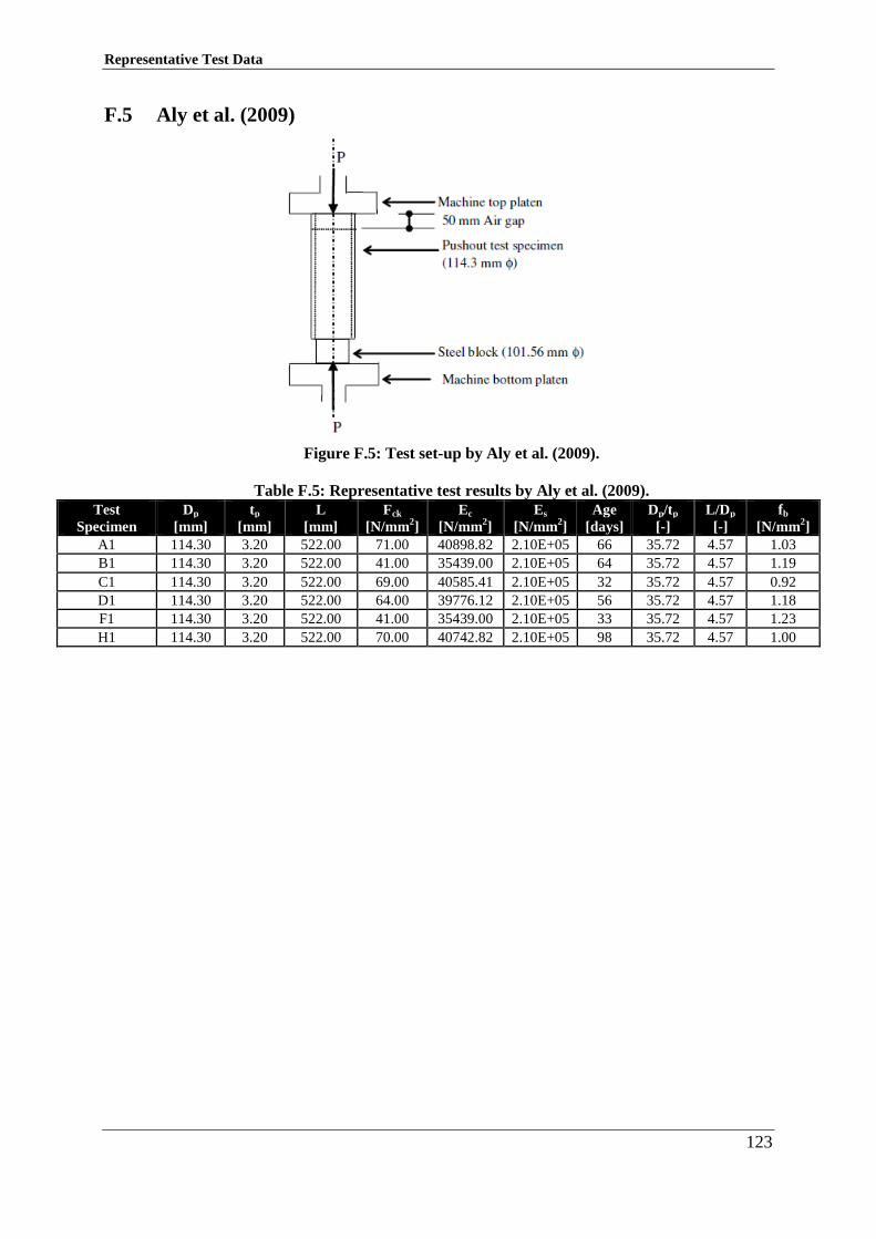
Representative Test Data
123
F.5 Aly et al. (2009)
Figure F.5: Test set-up by Aly et al. (2009).
Table F.5: Representative test results by Aly et al. (2009).
Test
Specimen
Dp
[mm]
tp
[mm]
L
[mm]
Fck
[N/mm2]
Ec
[N/mm2]
Es
[N/mm2]
Age
[days]
Dp/tp
[-]
L/Dp
[-]
fb
[N/mm2]
A1 114.30 3.20 522.00 71.00 40898.82 2.10E+05 66 35.72 4.57 1.03
B1 114.30 3.20 522.00 41.00 35439.00 2.10E+05 64 35.72 4.57 1.19
C1 114.30 3.20 522.00 69.00 40585.41 2.10E+05 32 35.72 4.57 0.92
D1 114.30 3.20 522.00 64.00 39776.12 2.10E+05 56 35.72 4.57 1.18
F1 114.30 3.20 522.00 41.00 35439.00 2.10E+05 33 35.72 4.57 1.23
H1 114.30 3.20 522.00 70.00 40742.82 2.10E+05 98 35.72 4.57 1.00

Representative Test Data
124
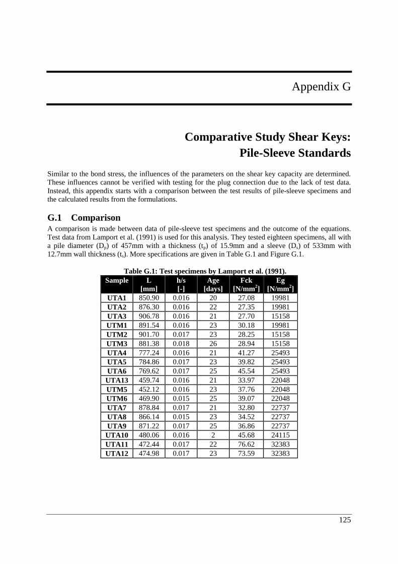
125
Appendix G
Appendix G Comparative Study Shear Keys:
Pile-Sleeve Standards
Similar to the bond stress, the influences of the parameters on the shear key capacity are determined.
These influences cannot be verified with testing for the plug connection due to the lack of test data.
Instead, this appendix starts with a comparison between the test results of pile-sleeve specimens and
the calculated results from the formulations.
G.1 Comparison A comparison is made between data of pile-sleeve test specimens and the outcome of the equations.
Test data from Lamport et al. (1991) is used for this analysis. They tested eighteen specimens, all with
a pile diameter (Dp) of 457mm with a thickness (tp) of 15.9mm and a sleeve (Ds) of 533mm with
12.7mm wall thickness (ts). More specifications are given in Table G.1 and Figure G.1.
Table G.1: Test specimens by Lamport et al. (1991).
Sample L
[mm]
h/s
[-]
Age
[days]
Fck
[N/mm2]
Eg
[N/mm2]
UTA1 850.90 0.016 20 27.08 19981
UTA2 876.30 0.016 22 27.35 19981
UTA3 906.78 0.016 21 27.70 15158
UTM1 891.54 0.016 23 30.18 19981
UTM2 901.70 0.017 23 28.25 15158
UTM3 881.38 0.018 26 28.94 15158
UTA4 777.24 0.016 21 41.27 25493
UTA5 784.86 0.017 23 39.82 25493
UTA6 769.62 0.017 25 45.54 25493
UTA13 459.74 0.016 21 33.97 22048
UTM5 452.12 0.016 23 37.76 22048
UTM6 469.90 0.015 25 39.07 22048
UTA7 878.84 0.017 21 32.80 22737
UTA8 866.14 0.015 23 34.52 22737
UTA9 871.22 0.017 25 36.86 22737
UTA10 480.06 0.016 2 45.68 24115
UTA11 472.44 0.017 22 76.62 32383
UTA12 474.98 0.017 23 73.59 32383
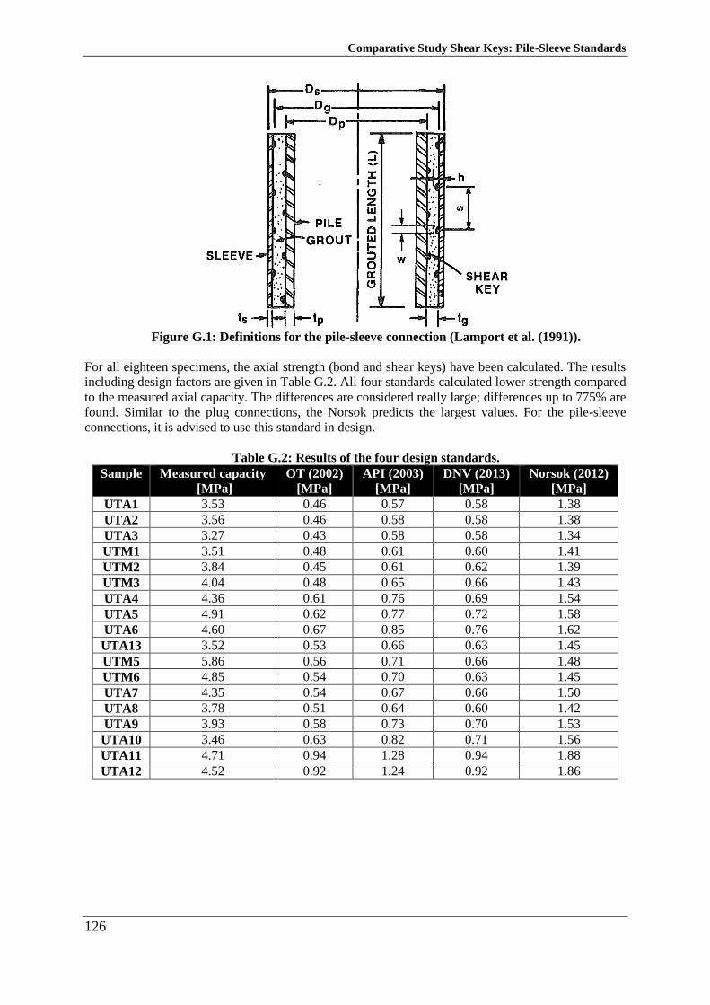
Comparative Study Shear Keys: Pile-Sleeve Standards
126
Figure G.1: Definitions for the pile-sleeve connection (Lamport et al. (1991)).
For all eighteen specimens, the axial strength (bond and shear keys) have been calculated. The results
including design factors are given in Table G.2. All four standards calculated lower strength compared
to the measured axial capacity. The differences are considered really large; differences up to 775% are
found. Similar to the plug connections, the Norsok predicts the largest values. For the pile-sleeve
connections, it is advised to use this standard in design.
Table G.2: Results of the four design standards.
Sample Measured capacity
[MPa]
OT (2002)
[MPa]
API (2003)
[MPa]
DNV (2013)
[MPa]
Norsok (2012)
[MPa]
UTA1 3.53 0.46 0.57 0.58 1.38
UTA2 3.56 0.46 0.58 0.58 1.38
UTA3 3.27 0.43 0.58 0.58 1.34
UTM1 3.51 0.48 0.61 0.60 1.41
UTM2 3.84 0.45 0.61 0.62 1.39
UTM3 4.04 0.48 0.65 0.66 1.43
UTA4 4.36 0.61 0.76 0.69 1.54
UTA5 4.91 0.62 0.77 0.72 1.58
UTA6 4.60 0.67 0.85 0.76 1.62
UTA13 3.52 0.53 0.66 0.63 1.45
UTM5 5.86 0.56 0.71 0.66 1.48
UTM6 4.85 0.54 0.70 0.63 1.45
UTA7 4.35 0.54 0.67 0.66 1.50
UTA8 3.78 0.51 0.64 0.60 1.42
UTA9 3.93 0.58 0.73 0.70 1.53
UTA10 3.46 0.63 0.82 0.71 1.56
UTA11 4.71 0.94 1.28 0.94 1.88
UTA12 4.52 0.92 1.24 0.92 1.86
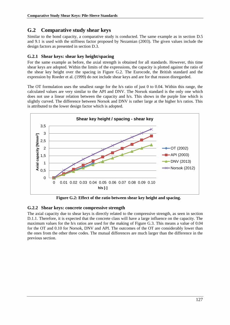
Comparative Study Shear Keys: Pile-Sleeve Standards
127
G.2 Comparative study shear keys Similar to the bond capacity, a comparative study is conducted. The same example as in section D.5
and 9.1 is used with the stiffness factor proposed by Nezamian (2003). The given values include the
design factors as presented in section D.3.
G.2.1 Shear keys: shear key height/spacing
For the same example as before, the axial strength is obtained for all standards. However, this time
shear keys are adopted. Within the limits of the expressions, the capacity is plotted against the ratio of
the shear key height over the spacing in Figure G.2. The Eurocode, the British standard and the
expression by Roeder et al. (1999) do not include shear keys and are for that reason disregarded.
The OT formulation uses the smallest range for the h/s ratio of just 0 to 0.04. Within this range, the
calculated values are very similar to the API and DNV. The Norsok standard is the only one which
does not use a linear relation between the capacity and h/s. This shows in the purple line which is
slightly curved. The difference between Norsok and DNV is rather large at the higher h/s ratios. This
is attributed to the lower design factor which is adopted.
Figure G.2: Effect of the ratio between shear key height and spacing.
G.2.2 Shear keys: concrete compressive strength
The axial capacity due to shear keys is directly related to the compressive strength, as seen in section
D.1.1. Therefore, it is expected that the concrete class will have a large influence on the capacity. The
maximum values for the h/s ratios are used for the making of Figure G.3. This means a value of 0.04
for the OT and 0.10 for Norsok, DNV and API. The outcomes of the OT are considerably lower than
the ones from the other three codes. The mutual differences are much larger than the difference in the
previous section.
0
0,5
1
1,5
2
2,5
3
3,5
0 0.01 0.02 0.03 0.04 0.05 0.06 0.07 0.08 0.09 0.10
Ax
ial
ca
pa
cit
y [
N/m
m2]
h/s [-]
Shear key height / spacing - shear key
OT (2002)
API (2003)
DNV (2013)
Norsok (2012)
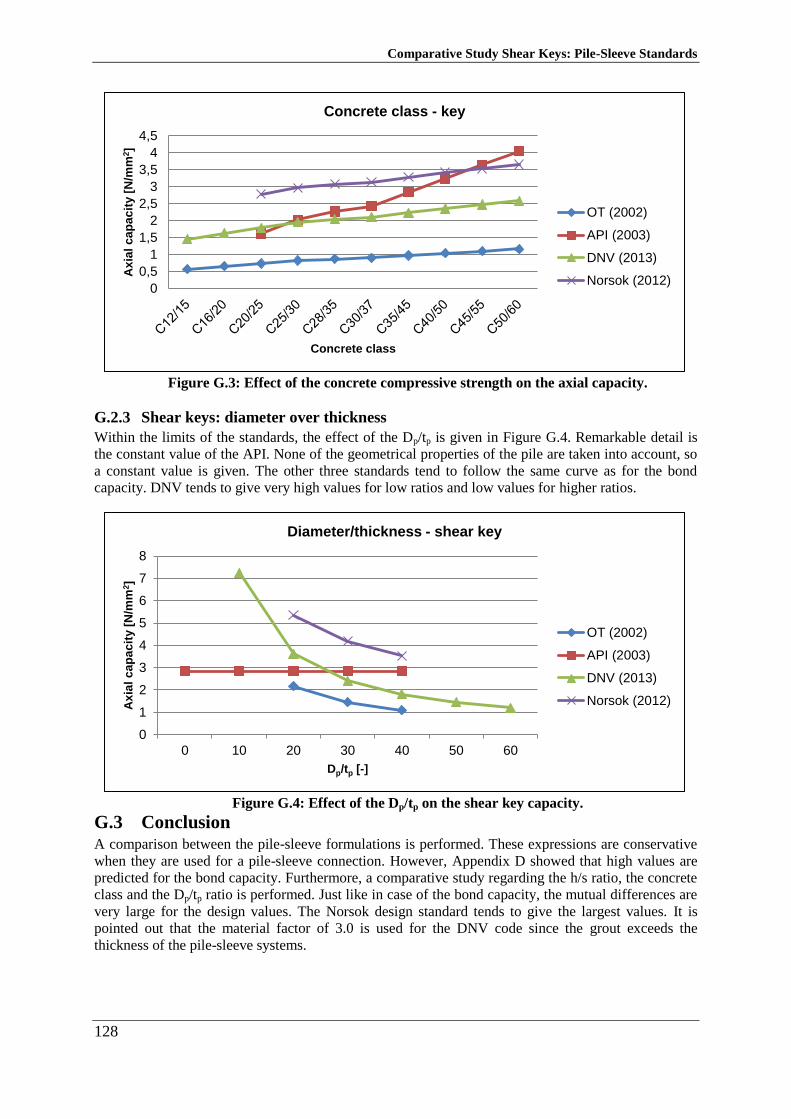
Comparative Study Shear Keys: Pile-Sleeve Standards
128
Figure G.3: Effect of the concrete compressive strength on the axial capacity.
G.2.3 Shear keys: diameter over thickness
Within the limits of the standards, the effect of the Dp/tp is given in Figure G.4. Remarkable detail is
the constant value of the API. None of the geometrical properties of the pile are taken into account, so
a constant value is given. The other three standards tend to follow the same curve as for the bond
capacity. DNV tends to give very high values for low ratios and low values for higher ratios.
Figure G.4: Effect of the Dp/tp on the shear key capacity.
G.3 Conclusion A comparison between the pile-sleeve formulations is performed. These expressions are conservative
when they are used for a pile-sleeve connection. However, Appendix D showed that high values are
predicted for the bond capacity. Furthermore, a comparative study regarding the h/s ratio, the concrete
class and the Dp/tp ratio is performed. Just like in case of the bond capacity, the mutual differences are
very large for the design values. The Norsok design standard tends to give the largest values. It is
pointed out that the material factor of 3.0 is used for the DNV code since the grout exceeds the
thickness of the pile-sleeve systems.
0
0,5
1
1,5
2
2,5
3
3,5
4
4,5A
xia
l c
ap
ac
ity [
N/m
m2]
Concrete class
Concrete class - key
OT (2002)
API (2003)
DNV (2013)
Norsok (2012)
0
1
2
3
4
5
6
7
8
0 10 20 30 40 50 60
Ax
ial
ca
pa
cit
y [
N/m
m2]
Dp/tp [-]
Diameter/thickness - shear key
OT (2002)
API (2003)
DNV (2013)
Norsok (2012)
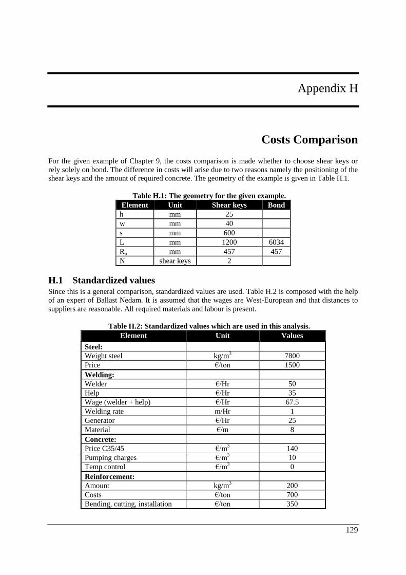
129
Appendix H
Appendix H Costs Comparison
For the given example of Chapter 9, the costs comparison is made whether to choose shear keys or
rely solely on bond. The difference in costs will arise due to two reasons namely the positioning of the
shear keys and the amount of required concrete. The geometry of the example is given in Table H.1.
Table H.1: The geometry for the given example.
Element Unit Shear keys Bond
h mm 25
w mm 40
s mm 600
L mm 1200 6034
Rp mm 457 457
N shear keys 2
H.1 Standardized values Since this is a general comparison, standardized values are used. Table H.2 is composed with the help
of an expert of Ballast Nedam. It is assumed that the wages are West-European and that distances to
suppliers are reasonable. All required materials and labour is present.
Table H.2: Standardized values which are used in this analysis.
Element Unit Values
Steel:
Weight steel kg/m3
7800
Price €/ton 1500
Welding:
Welder €/Hr 50
Help €/Hr 35
Wage (welder + help) €/Hr 67.5
Welding rate m/Hr 1
Generator €/Hr 25
Material €/m 8
Concrete:
Price C35/45 €/m3
140
Pumping charges €/m3 10
Temp control €/m3
0
Reinforcement:
Amount kg/m3 200
Costs €/ton 700
Bending, cutting, installation €/ton 350
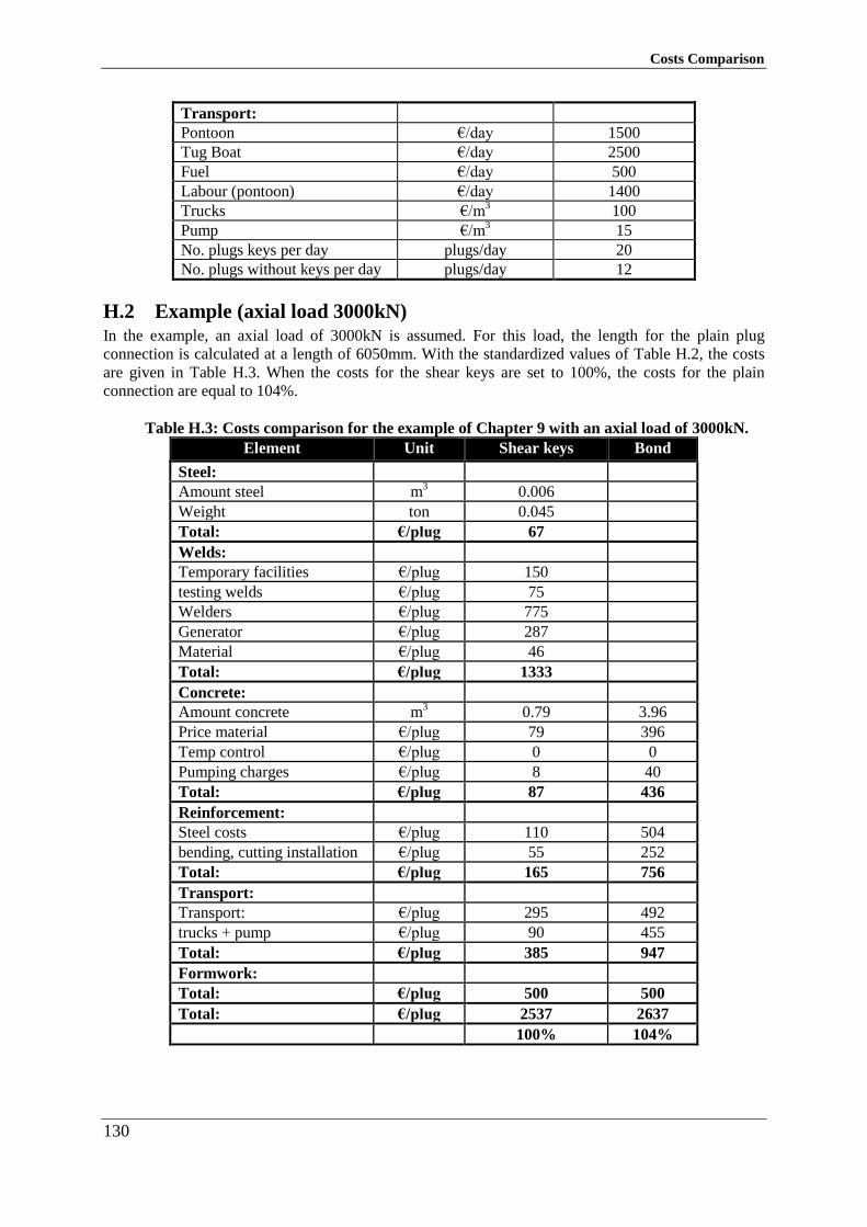
Costs Comparison
130
Transport:
Pontoon €/day 1500
Tug Boat €/day 2500
Fuel €/day 500
Labour (pontoon) €/day 1400
Trucks €/m3 100
Pump €/m3
15
No. plugs keys per day plugs/day 20
No. plugs without keys per day plugs/day 12
H.2 Example (axial load 3000kN) In the example, an axial load of 3000kN is assumed. For this load, the length for the plain plug
connection is calculated at a length of 6050mm. With the standardized values of Table H.2, the costs
are given in Table H.3. When the costs for the shear keys are set to 100%, the costs for the plain
connection are equal to 104%.
Table H.3: Costs comparison for the example of Chapter 9 with an axial load of 3000kN.
Element Unit Shear keys Bond
Steel:
Amount steel m3 0.006
Weight ton 0.045
Total: €/plug 67
Welds:
Temporary facilities €/plug 150
testing welds €/plug 75
Welders €/plug 775
Generator €/plug 287
Material €/plug 46
Total: €/plug 1333
Concrete:
Amount concrete m3 0.79 3.96
Price material €/plug 79 396
Temp control €/plug 0 0
Pumping charges €/plug 8 40
Total: €/plug 87 436
Reinforcement:
Steel costs €/plug 110 504
bending, cutting installation €/plug 55 252
Total: €/plug 165 756
Transport:
Transport: €/plug 295 492
trucks + pump €/plug 90 455
Total: €/plug 385 947
Formwork:
Total: €/plug 500 500
Total: €/plug 2537 2637
100% 104%
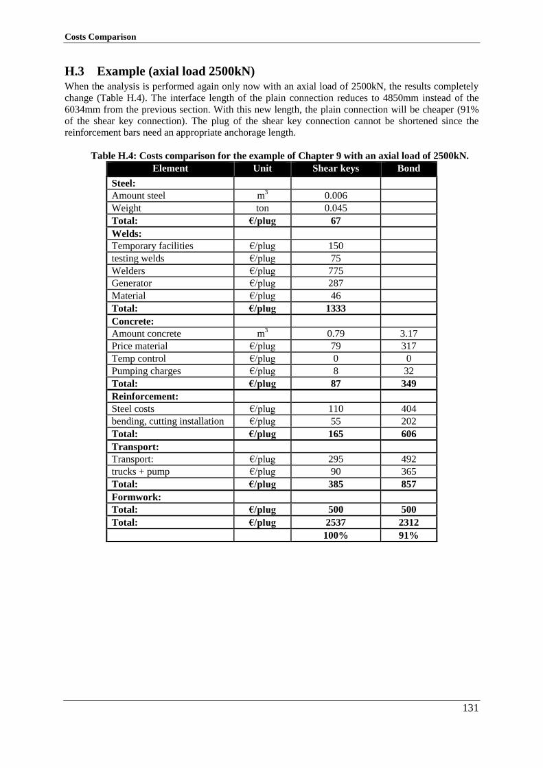
Costs Comparison
131
H.3 Example (axial load 2500kN) When the analysis is performed again only now with an axial load of 2500kN, the results completely
change (Table H.4). The interface length of the plain connection reduces to 4850mm instead of the
6034mm from the previous section. With this new length, the plain connection will be cheaper (91%
of the shear key connection). The plug of the shear key connection cannot be shortened since the
reinforcement bars need an appropriate anchorage length.
Table H.4: Costs comparison for the example of Chapter 9 with an axial load of 2500kN.
Element Unit Shear keys Bond
Steel:
Amount steel m3 0.006
Weight ton 0.045
Total: €/plug 67
Welds:
Temporary facilities €/plug 150
testing welds €/plug 75
Welders €/plug 775
Generator €/plug 287
Material €/plug 46
Total: €/plug 1333
Concrete:
Amount concrete m3 0.79 3.17
Price material €/plug 79 317
Temp control €/plug 0 0
Pumping charges €/plug 8 32
Total: €/plug 87 349
Reinforcement:
Steel costs €/plug 110 404
bending, cutting installation €/plug 55 202
Total: €/plug 165 606
Transport:
Transport: €/plug 295 492
trucks + pump €/plug 90 365
Total: €/plug 385 857
Formwork:
Total: €/plug 500 500
Total: €/plug 2537 2312
100% 91%
Costs Comparison
132
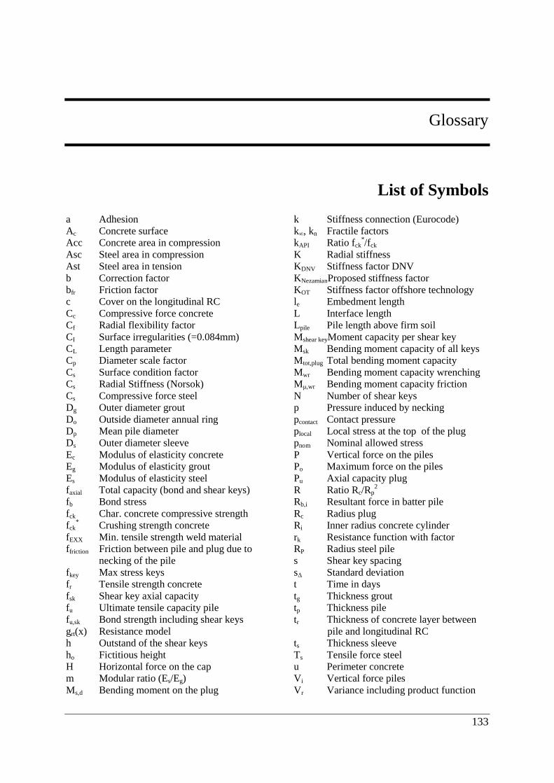
133
Glossary
Appendix I List of Symbols
a Adhesion
Ac Concrete surface
Acc Concrete area in compression
Asc Steel area in compression
Ast Steel area in tension
b Correction factor
bfr Friction factor
c Cover on the longitudinal RC
Cc Compressive force concrete
Cf Radial flexibility factor
CI Surface irregularities (=0.084mm)
CL Length parameter
Cp Diameter scale factor
Cs Surface condition factor
Cs Radial Stiffness (Norsok)
Cs Compressive force steel
Dg Outer diameter grout
Do Outside diameter annual ring
Dp Mean pile diameter
Ds Outer diameter sleeve
Ec Modulus of elasticity concrete
Eg Modulus of elasticity grout
Es Modulus of elasticity steel
faxial Total capacity (bond and shear keys)
fb Bond stress
fck Char. concrete compressive strength
fck* Crushing strength concrete
fEXX Min. tensile strength weld material
ffriction Friction between pile and plug due to
necking of the pile
fkey Max stress keys
fr Tensile strength concrete
fsk Shear key axial capacity
fu Ultimate tensile capacity pile
fu,sk Bond strength including shear keys
grt(x) Resistance model
h Outstand of the shear keys
ho Fictitious height
H Horizontal force on the cap
m Modular ratio (Es/Eg)
Ms,d Bending moment on the plug
k Stiffness connection (Eurocode)
k∞, kn Fractile factors
kAPI Ratio fck*/fck
K Radial stiffness
KDNV Stiffness factor DNV
KNezamianProposed stiffness factor
KOT Stiffness factor offshore technology
le Embedment length
L Interface length
Lpile Pile length above firm soil
Mshear keyMoment capacity per shear key
Msk Bending moment capacity of all keys
Mtot,plug Total bending moment capacity
Mwr Bending moment capacity wrenching
Mμ,wr Bending moment capacity friction
N Number of shear keys
p Pressure induced by necking
pcontact Contact pressure
plocal Local stress at the top of the plug
pnom Nominal allowed stress
P Vertical force on the piles
Po Maximum force on the piles
Pu Axial capacity plug
R Ratio Rc/Rp2
Rb,i Resultant force in batter pile
Rc Radius plug
Ri Inner radius concrete cylinder
rk Resistance function with factor
RP Radius steel pile
s Shear key spacing
sΔ Standard deviation
t Time in days
tg Thickness grout
tp Thickness pile
tr Thickness of concrete layer between
pile and longitudinal RC
ts Thickness sleeve
Ts Tensile force steel
u Perimeter concrete
Vi Vertical force piles
Vr Variance including product function
Glossary
134
Vxi Variance resistance factors
Vδ Variance test data
w Shear key width
W Weld size
Greek Symbols
αrt, αδ Weighing factors
α, β, κ Empirical parameters Kelvin model
βas Time factor autogenous shrinkage
βds(t,ts) Time factor chemical shrinkage
δDNV Surface condition DNV (0.0037Rp)
δi Specimen dispersion
Δ Difference in radial displacements
Δ- Average dispersion
Δ1 Enlargement of the steel tube
Δ2 Shrinkage
Δ3 Rugosity of the tube
Δc Radial displacement concrete
Δi Logarithm of dispersion terms
Δs Radial displacement steel
εac(∞) Final autogenous shrinkage
εcd(t) Chemical shrinkage
εc,θ Circumferential strain concrete
εs,θ Circumferential strain steel
κ Early age reduction factor (DNV)
μ Coulomb-friction coefficient (=0.5)
μs Surface irregularities tube (=0.05)
μDNV Surface interface DNV (=0.4-0.6)
υc Poisson ratio concrete
υs Poisson ratio steel
ρv Amount of shear RC
σc,n Radial pressure on the concrete
σc,θ Circumferential stress concrete
σc,z Longitudinal stress concrete
σs,n Radial pressure on the steel tube
σs,θ Circumferential stress steel tube
σs,z Longitudinal stress steel tube
τ Shear strength concrete
τA Axial shear due to normal force
τM Axial shear due to bending moment
τkg Shear strength grout
φ Angle
Appendix J List of Acronyms
API American Petroleum Institute
BS British Standard
CFT Concrete Filled Tube
DF Derived Formulation
DNV Det Norske Veritas
EC Eurocode
FE Finite Element
MOE Modulus of Elasticity
NSC Normal Strength Concrete
OT Offshore Technology
PSDM Plastic Stress Distribution Method
RC Reinforcement
SD Standard Deviation
SCF Stress Concentration Factor
STM Strut and Tie Model