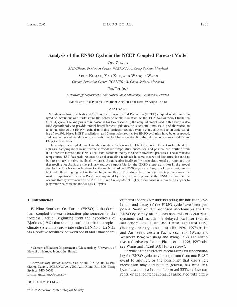
Analysis of the ENSO Cycle in the NCEP Coupled Forecast Model

QIN ZHANG

RSIS/Climate Prediction Center, NCEP/NOAA, Camp Springs, Maryland

ARUN KUMAR, YAN XUE, AND WANQIU WANG

Climate Prediction Center, NCEP/NOAA, Camp Springs, Maryland

FEI-FEI JIN*Meteorology Department, The Florida State University, Tallahassee, Florida

(Manuscript received 30 November 2005, in final form 29 August 2006)

ABSTRACT

Simulations from the National Centers for Environmental Prediction (NCEP) coupled model are ana-lyzed to document and understand the behavior of the evolution of the El Niño–Southern Oscillation(ENSO) cycle. The analysis is of importance for two reasons: 1) the coupled model used in this study is alsoused operationally to provide model-based forecast guidance on a seasonal time scale, and therefore, anunderstanding of the ENSO mechanism in this particular coupled system could also lead to an understand-ing of possible biases in SST predictions; and 2) multiple theories for ENSO evolution have been proposed,and coupled model simulations are a useful test bed for understanding the relative importance of differentENSO mechanisms.

The analyses of coupled model simulations show that during the ENSO evolution the net surface heat fluxacts as a damping mechanism for the mixed-layer temperature anomalies, and positive contribution fromthe advection terms to the ENSO evolution is dominated by the linear advective processes. The subsurfacetemperature–SST feedback, referred to as thermocline feedback in some theoretical literature, is found tobe the primary positive feedback, whereas the advective feedback by anomalous zonal currents and thethermocline feedback are the primary sources responsible for the ENSO phase transition in the modelsimulation. The basic mechanisms for the model-simulated ENSO cycle are thus, to a large extent, consis-tent with those highlighted in the recharge oscillator. The atmospheric anticyclone (cyclone) over thewestern equatorial northern Pacific accompanied by a warm (cold) phase of the ENSO, as well as theoceanic Rossby waves outside of 15°S–15°N and the equatorial higher-order baroclinic modes, all appear toplay minor roles in the model ENSO cycles.

1. Introduction

El Niño–Southern Oscillation (ENSO) is the domi-nant coupled air–sea interaction phenomenon in thetropical Pacific. Beginning from the hypothesis ofBjerknes (1969) that small perturbations in the tropicalclimate system may grow into either El Niño or La Niñavia a positive feedback between ocean and atmosphere,

different theories for understanding the initiation, evo-lution, and decay of the ENSO cycle have been pro-posed. Some of the proposed mechanisms for theENSO cycle rely on the dominant role of ocean wavedynamics and include the delayed oscillator (Suarezand Schopf 1988; Hirst 1988; Battisti and Hirst 1989),discharge–recharge oscillator (Jin 1996, 1997a,b; Jinand An 1999), western Pacific oscillator (Wang andWeisberg 1994; Weisberg and Wang 1997), and advec-tive–reflective oscillator (Picaut et al. 1996, 1997; alsosee Wang and Picaut 2004 for a review).

To what extent different mechanisms for understand-ing the ENSO cycle may be important from one ENSOevent to another, or the possibility that one singlemechanism may dominate in general, has been ana-lyzed based on evolution of observed SSTs, surface cur-rents, or heat content anomalies associated with differ-

* Current affiliation: Department of Meteorology, University ofHawaii at Manoa, Honolulu, Hawaii.

Corresponding author address: Qin Zhang, RSIS/Climate Pre-diction Center, NCEP/NOAA, 5200 Auth Road, Rm. 800, CampSprings, MD 20746.E-mail: qin.zhang@noaa.gov

1 APRIL 2007 Z H A N G E T A L . 1265

DOI: 10.1175/JCLI4062.1

© 2007 American Meteorological Society

JCLI4062

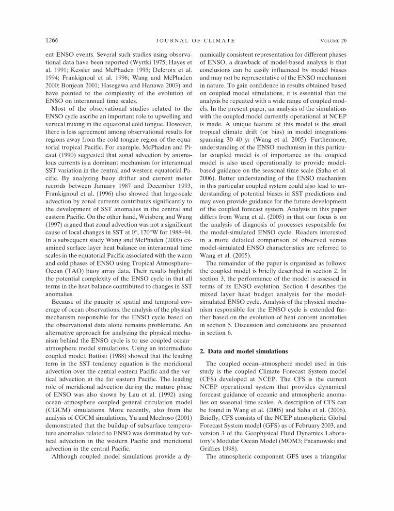
ent ENSO events. Several such studies using observa-tional data have been reported (Wyrtki 1975; Hayes etal. 1991; Kessler and McPhaden 1995; Delcroix et al.1994; Frankignoul et al. 1996; Wang and McPhaden2000; Bonjean 2001; Hasegawa and Hanawa 2003) andhave pointed to the complexity of the evolution ofENSO on interannual time scales.

Most of the observational studies related to theENSO cycle ascribe an important role to upwelling andvertical mixing in the equatorial cold tongue. However,there is less agreement among observational results forregions away from the cold tongue region of the equa-torial tropical Pacific. For example, McPhaden and Pi-caut (1990) suggested that zonal advection by anoma-lous currents is a dominant mechanism for interannualSST variation in the central and western equatorial Pa-cific. By analyzing buoy drifter and current meterrecords between January 1987 and December 1993,Frankignoul et al. (1996) also showed that large-scaleadvection by zonal currents contributes significantly tothe development of SST anomalies in the central andeastern Pacific. On the other hand, Weisberg and Wang(1997) argued that zonal advection was not a significantcause of local changes in SST at 0°, 170°W for 1988–94.In a subsequent study Wang and McPhaden (2000) ex-amined surface layer heat balance on interannual timescales in the equatorial Pacific associated with the warmand cold phases of ENSO using Tropical Atmosphere–Ocean (TAO) buoy array data. Their results highlightthe potential complexity of the ENSO cycle in that allterms in the heat balance contributed to changes in SSTanomalies.

Because of the paucity of spatial and temporal cov-erage of ocean observations, the analysis of the physicalmechanism responsible for the ENSO cycle based onthe observational data alone remains problematic. Analternative approach for analyzing the physical mecha-nism behind the ENSO cycle is to use coupled ocean–atmosphere model simulations. Using an intermediatecoupled model, Battisti (1988) showed that the leadingterm in the SST tendency equation is the meridionaladvection over the central-eastern Pacific and the ver-tical advection at the far eastern Pacific. The leadingrole of meridional advection during the mature phaseof ENSO was also shown by Lau et al. (1992) usingocean–atmosphere coupled general circulation model(CGCM) simulations. More recently, also from theanalysis of CGCM simulations, Yu and Mechoso (2001)demonstrated that the buildup of subsurface tempera-ture anomalies related to ENSO was dominated by ver-tical advection in the western Pacific and meridionaladvection in the central Pacific.

Although coupled model simulations provide a dy-

namically consistent representation for different phasesof ENSO, a drawback of model-based analysis is thatconclusions can be easily influenced by model biasesand may not be representative of the ENSO mechanismin nature. To gain confidence in results obtained basedon coupled model simulations, it is essential that theanalysis be repeated with a wide range of coupled mod-els. In the present paper, an analysis of the simulationswith the coupled model currently operational at NCEPis made. A unique feature of this model is the smalltropical climate drift (or bias) in model integrationsspanning 30–40 yr (Wang et al. 2005). Furthermore,understanding of the ENSO mechanism in this particu-lar coupled model is of importance as the coupledmodel is also used operationally to provide model-based guidance on the seasonal time scale (Saha et al.2006). Better understanding of the ENSO mechanismin this particular coupled system could also lead to un-derstanding of potential biases in SST predictions andmay even provide guidance for the future developmentof the coupled forecast system. Analysis in this paperdiffers from Wang et al. (2005) in that our focus is onthe analysis of diagnosis of processes responsible forthe model-simulated ENSO cycle. Readers interestedin a more detailed comparison of observed versusmodel-simulated ENSO characteristics are referred toWang et al. (2005).

The remainder of the paper is organized as follows:the coupled model is briefly described in section 2. Insection 3, the performance of the model is assessed interms of its ENSO evolution. Section 4 describes themixed layer heat budget analysis for the model-simulated ENSO cycle. Analysis of the physical mecha-nism responsible for the ENSO cycle is extended fur-ther based on the evolution of heat content anomaliesin section 5. Discussion and conclusions are presentedin section 6.

2. Data and model simulations

The coupled ocean–atmosphere model used in thisstudy is the coupled Climate Forecast System model(CFS) developed at NCEP. The CFS is the currentNCEP operational system that provides dynamicalforecast guidance of oceanic and atmospheric anoma-lies on seasonal time scales. A description of CFS canbe found in Wang et al. (2005) and Saha et al. (2006).Briefly, CFS consists of the NCEP atmospheric GlobalForecast System model (GFS) as of February 2003, andversion 3 of the Geophysical Fluid Dynamics Labora-tory’s Modular Ocean Model (MOM3; Pacanowski andGriffies 1998).

The atmospheric component GFS uses a triangular

1266 J O U R N A L O F C L I M A T E VOLUME 20

horizontal spectral truncation of 62 waves (T62) andhas 64 vertical levels with enhanced resolution near thelower and the upper boundaries of the vertical domain.The top-most boundary of the model extends to 0.2hPa. The model also includes a comprehensive packageof parameterization schemes related to different atmo-spheric processes.

The MOM3 ocean model is configured as a globalocean model with north–south domain extending from74°S to 64°N. The model has 40 layers in the verticalwith 10-m resolution in the upper 240 m. Latitudinalspacing is 1/3° between 10°S and 10°N, gradually in-creasing through the Tropics until becoming fixed 1°poleward of 30°S and 30°N. The longitudinal spacing is1°. Vertical mixing follows the nonlocal K-profile pa-rameterization of Large et al. (1994). The horizontalmixing of tracers uses the isoneutral method pioneeredby Gent and McWilliams (1990; see also Griffies et al.1998). The horizontal mixing of momentum uses thenonlinear scheme of Smagorinsky (1963).

The atmospheric and oceanic components arecoupled without any flux adjustment. The two compo-nents exchange daily averaged quantities once per day.Because of the difference in latitudinal domain, fullinteraction between atmospheric and oceanic compo-nents is confined to 65°S to 50°N. Poleward of 74°S and64°N, SSTs for the atmospheric component are takenfrom observed climatology. Between 74° and 65°S, and64° and 50°N, SSTs for the atmospheric component arethe weighted average of the observed SST climatologyand the SST from the ocean component of CFS, withweights linearly varying in latitude such that SSTs at74°S and 64°N equal the observed climatology, and at65°S to 50°N equal SSTs from the ocean model. Sea iceextent is prescribed from the observed climatology.

In the present study a set of three 30-yr coupledsimulations is analyzed. These simulations started frominitial conditions of 1 January of 1988, 1995, and 2002.The oceanic initial states were taken from the NCEPGlobal Ocean and Data Assimilation System (GODAS)and the atmospheric initial conditions from the NCEP/Department of Energy (DOE) Reanalysis-2 (Kana-mitsu et al. 2002). Each of the three coupled modelintegrations is for a 40-yr period, and the first 10 yr ofthe model integration are not included in the analysis.This allows analysis of data after the coupled modelsimulations have entered their state of climatologicalinterannual variability. Although the model drift forthe first 40 yr of integrations is small, to avoid compli-cations due to larger potential drift that may exist inlonger integrations, we restrict each coupled integra-tion to a 40-yr period. Our analysis is based on monthly

mean fields and all anomalies are computed with re-spect to each model’s own climatology.

3. Coupled model simulation of the ENSOvariability

Prior to presenting the heat budget analysis, theENSO cycle in the coupled model simulation is de-scribed. The analysis complements the analysis ofWang et al. (2005), who for the same coupled modelsimulations, also discussed some basic features ofmodel biases and simulation of the ENSO variability.

For the three coupled simulations we first identifythe ENSO events. Model ENSO events are identifiedbased on the time series of the model-simulated Niño-3.4 SST index. Specifically, whenever a warm, as well asthe subsequent cold, peak in the Niño-3.4 time seriesexceeds one standard deviation, a warm event followedby a cold event (referred to as the ENSO cycle) is iden-tified. If a warm or cold event occurs in isolation, suchisolated events are not included in our analysis, a sce-nario that occurs quite infrequently. Based on this cri-terion, a total of 14 warm–cold ENSO cycle events areidentified.

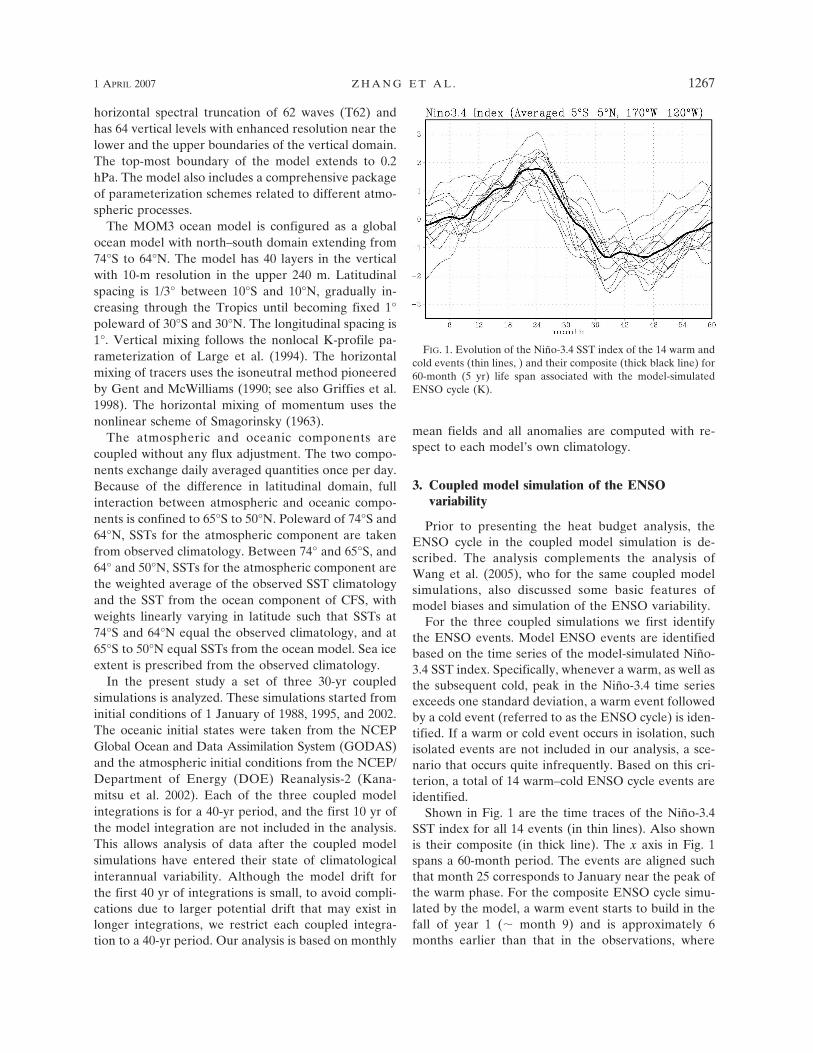
Shown in Fig. 1 are the time traces of the Niño-3.4SST index for all 14 events (in thin lines). Also shownis their composite (in thick line). The x axis in Fig. 1spans a 60-month period. The events are aligned suchthat month 25 corresponds to January near the peak ofthe warm phase. For the composite ENSO cycle simu-lated by the model, a warm event starts to build in thefall of year 1 (� month 9) and is approximately 6months earlier than that in the observations, where

FIG. 1. Evolution of the Niño-3.4 SST index of the 14 warm andcold events (thin lines, ) and their composite (thick black line) for60-month (5 yr) life span associated with the model-simulatedENSO cycle (K).

1 APRIL 2007 Z H A N G E T A L . 1267

warm events start to develop around March of year 2(month 15; Rasmusson and Carpenter 1982). The warmNiño-3.4 SST anomalies reach their peak during thenorthern winter of years 2/3, following which the Niño-3.4 anomaly evolves to a cold phase. The duration ofthe peak in the cold Niño-3.4 SST anomalies is broadercompared to the warm events, and furthermore, similarto the observations, it is weaker in amplitude than forthe warm event.

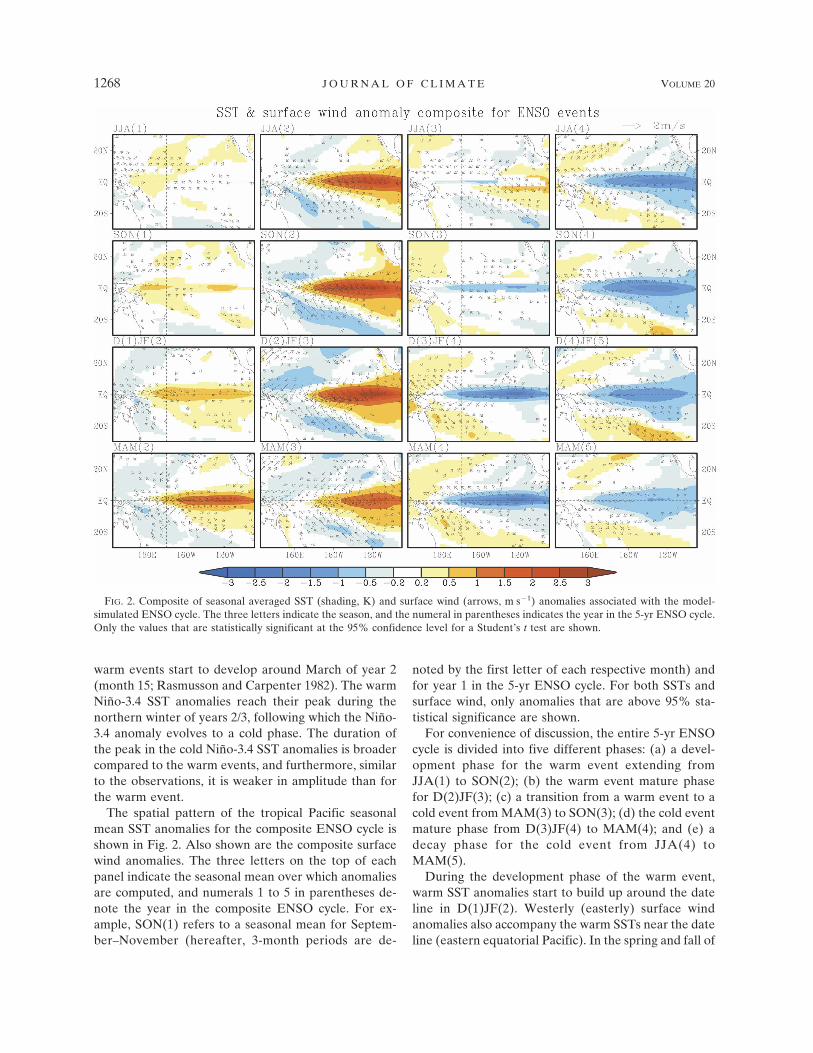
The spatial pattern of the tropical Pacific seasonalmean SST anomalies for the composite ENSO cycle isshown in Fig. 2. Also shown are the composite surfacewind anomalies. The three letters on the top of eachpanel indicate the seasonal mean over which anomaliesare computed, and numerals 1 to 5 in parentheses de-note the year in the composite ENSO cycle. For ex-ample, SON(1) refers to a seasonal mean for Septem-ber–November (hereafter, 3-month periods are de-

noted by the first letter of each respective month) andfor year 1 in the 5-yr ENSO cycle. For both SSTs andsurface wind, only anomalies that are above 95% sta-tistical significance are shown.

For convenience of discussion, the entire 5-yr ENSOcycle is divided into five different phases: (a) a devel-opment phase for the warm event extending fromJJA(1) to SON(2); (b) the warm event mature phasefor D(2)JF(3); (c) a transition from a warm event to acold event from MAM(3) to SON(3); (d) the cold eventmature phase from D(3)JF(4) to MAM(4); and (e) adecay phase for the cold event from JJA(4) toMAM(5).

During the development phase of the warm event,warm SST anomalies start to build up around the dateline in D(1)JF(2). Westerly (easterly) surface windanomalies also accompany the warm SSTs near the dateline (eastern equatorial Pacific). In the spring and fall of

FIG. 2. Composite of seasonal averaged SST (shading, K) and surface wind (arrows, m s�1) anomalies associated with the model-simulated ENSO cycle. The three letters indicate the season, and the numeral in parentheses indicates the year in the 5-yr ENSO cycle.Only the values that are statistically significant at the 95% confidence level for a Student’s t test are shown.

1268 J O U R N A L O F C L I M A T E VOLUME 20

Fig 2 live 4/C

year 2, weak SST anomalies amplify and spreadthroughout the equatorial tropical Pacific. Strengthen-ing of warm SSTs is also associated with the strength-ening of westerly wind anomalies throughout the Pa-cific basin with the exception of anomalous easterliesconfined near the west coast of South America. Inphase with the warming of the equatorial SSTs, well-defined cold SST anomalies in the form of a horseshoepattern, straddling the warm SSTs, also begin to estab-lish. Warm SST anomalies peak around December ofyear 2. A particular feature to note is that the warmestanomalies are located around 150°W, and not close tothe South American coast. At the peak of the warmevent around D(2)JF(3), easterly surface wind anoma-lies also appear over the warm pool, and consistent withthe observations, are associated with the establishmentof an anticyclone over the Philippine Sea (Wang et al.2000; Wang and Zhang 2002).

Following the peak phase of the warm event in thewinter of years 2/3, SST anomalies start to decrease andtransition to the cold phase of the ENSO cycle. BySON(3) the westerly surface wind anomalies are re-placed by the easterly anomalies throughout the equa-torial tropical Pacific. For the ENSO cycle simulated bythe coupled model, the mature phase of cold event lastsalmost through year 4, and has a broader peak than thatcorresponding for the warm event. The cold SSTanomalies in the eastern Pacific and warm SST anoma-lies in the western Pacific, as well as the anomalies offthe equatorial latitudes, are almost opposite to the SSTconditions during the warm phase of the ENSO cycle.Finally, in year 4 of the ENSO cycle, the cold SSTanomalies gradually start to decrease and reach neutralconditions by the end of year 5 (Fig. 1).

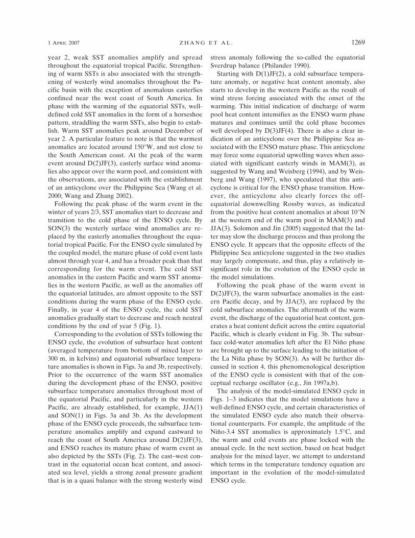
Corresponding to the evolution of SSTs following theENSO cycle, the evolution of subsurface heat content(averaged temperature from bottom of mixed layer to300 m, in kelvins) and equatorial subsurface tempera-ture anomalies is shown in Figs. 3a and 3b, respectively.Prior to the occurrence of the warm SST anomaliesduring the development phase of the ENSO, positivesubsurface temperature anomalies throughout most ofthe equatorial Pacific, and particularly in the westernPacific, are already established, for example, JJA(1)and SON(1) in Figs. 3a and 3b. As the developmentphase of the ENSO cycle proceeds, the subsurface tem-perature anomalies amplify and expand eastward toreach the coast of South America around D(2)JF(3),and ENSO reaches its mature phase of warm event asalso depicted by the SSTs (Fig. 2). The east–west con-trast in the equatorial ocean heat content, and associ-ated sea level, yields a strong zonal pressure gradientthat is in a quasi balance with the strong westerly wind

stress anomaly following the so-called the equatorialSverdrup balance (Philander 1990).

Starting with D(1)JF(2), a cold subsurface tempera-ture anomaly, or negative heat content anomaly, alsostarts to develop in the western Pacific as the result ofwind stress forcing associated with the onset of thewarming. This initial indication of discharge of warmpool heat content intensifies as the ENSO warm phasematures and continues until the cold phase becomeswell developed by D(3)JF(4). There is also a clear in-dication of an anticyclone over the Philippine Sea as-sociated with the ENSO mature phase. This anticyclonemay force some equatorial upwelling waves when asso-ciated with significant easterly winds in MAM(3), assuggested by Wang and Weisberg (1994), and by Weis-berg and Wang (1997), who speculated that this anti-cyclone is critical for the ENSO phase transition. How-ever, the anticyclone also clearly forces the off-equatorial downwelling Rossby waves, as indicatedfrom the positive heat content anomalies at about 10°Nat the western end of the warm pool in MAM(3) andJJA(3). Solomon and Jin (2005) suggested that the lat-ter may slow the discharge process and thus prolong theENSO cycle. It appears that the opposite effects of thePhilippine Sea anticyclone suggested in the two studiesmay largely compensate, and thus, play a relatively in-significant role in the evolution of the ENSO cycle inthe model simulations.

Following the peak phase of the warm event inD(2)JF(3), the warm subsurface anomalies in the east-ern Pacific decay, and by JJA(3), are replaced by thecold subsurface anomalies. The aftermath of the warmevent, the discharge of the equatorial heat content, gen-erates a heat content deficit across the entire equatorialPacific, which is clearly evident in Fig. 3b. The subsur-face cold-water anomalies left after the El Niño phaseare brought up to the surface leading to the initiation ofthe La Niña phase by SON(3). As will be further dis-cussed in section 4, this phenomenological descriptionof the ENSO cycle is consistent with that of the con-ceptual recharge oscillator (e.g., Jin 1997a,b).

The analysis of the model-simulated ENSO cycle inFigs. 1–3 indicates that the model simulations have awell-defined ENSO cycle, and certain characteristics ofthe simulated ENSO cycle also match their observa-tional counterparts. For example, the amplitude of theNiño-3.4 SST anomalies is approximately 1.5°C, andthe warm and cold events are phase locked with theannual cycle. In the next section, based on heat budgetanalysis for the mixed layer, we attempt to understandwhich terms in the temperature tendency equation areimportant in the evolution of the model-simulatedENSO cycle.

1 APRIL 2007 Z H A N G E T A L . 1269

4. Mixed-layer heat budget associated with ENSO

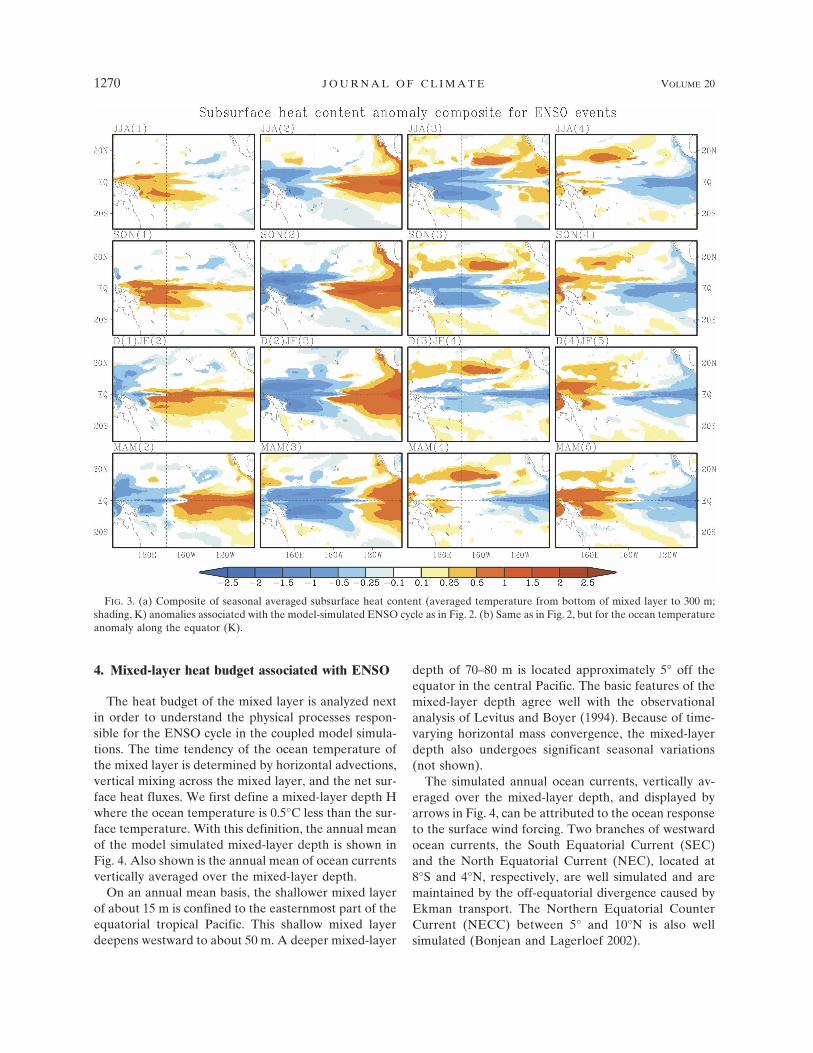
The heat budget of the mixed layer is analyzed nextin order to understand the physical processes respon-sible for the ENSO cycle in the coupled model simula-tions. The time tendency of the ocean temperature ofthe mixed layer is determined by horizontal advections,vertical mixing across the mixed layer, and the net sur-face heat fluxes. We first define a mixed-layer depth Hwhere the ocean temperature is 0.5°C less than the sur-face temperature. With this definition, the annual meanof the model simulated mixed-layer depth is shown inFig. 4. Also shown is the annual mean of ocean currentsvertically averaged over the mixed-layer depth.

On an annual mean basis, the shallower mixed layerof about 15 m is confined to the easternmost part of theequatorial tropical Pacific. This shallow mixed layerdeepens westward to about 50 m. A deeper mixed-layer

depth of 70–80 m is located approximately 5° off theequator in the central Pacific. The basic features of themixed-layer depth agree well with the observationalanalysis of Levitus and Boyer (1994). Because of time-varying horizontal mass convergence, the mixed-layerdepth also undergoes significant seasonal variations(not shown).

The simulated annual ocean currents, vertically av-eraged over the mixed-layer depth, and displayed byarrows in Fig. 4, can be attributed to the ocean responseto the surface wind forcing. Two branches of westwardocean currents, the South Equatorial Current (SEC)and the North Equatorial Current (NEC), located at8°S and 4°N, respectively, are well simulated and aremaintained by the off-equatorial divergence caused byEkman transport. The Northern Equatorial CounterCurrent (NECC) between 5° and 10°N is also wellsimulated (Bonjean and Lagerloef 2002).

FIG. 3. (a) Composite of seasonal averaged subsurface heat content (averaged temperature from bottom of mixed layer to 300 m;shading, K) anomalies associated with the model-simulated ENSO cycle as in Fig. 2. (b) Same as in Fig. 2, but for the ocean temperatureanomaly along the equator (K).

1270 J O U R N A L O F C L I M A T E VOLUME 20

Fig 3a live 4/C

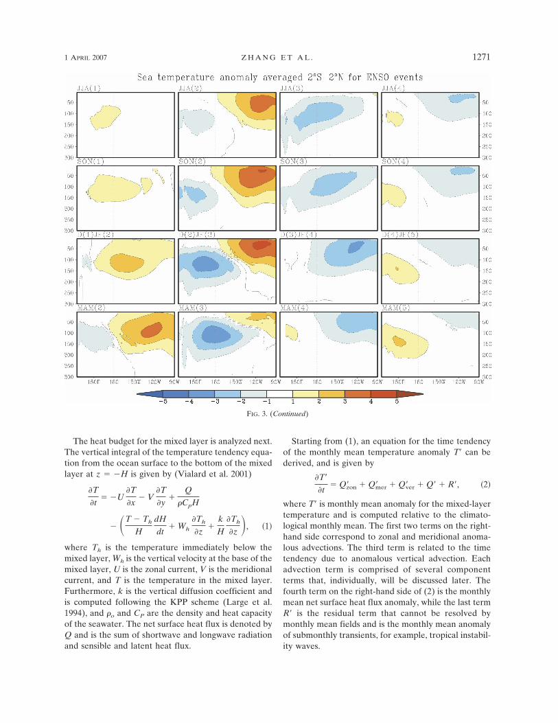
The heat budget for the mixed layer is analyzed next.The vertical integral of the temperature tendency equa-tion from the ocean surface to the bottom of the mixedlayer at z � �H is given by (Vialard et al. 2001)

�T

�t� �U

�T

�x� V

�T

�y�

Q

�CpH

� �T � Th

H

dH

dt� Wh

�Th

�z�

k

H

�Th

�z �, �1�

where Th is the temperature immediately below themixed layer, Wh is the vertical velocity at the base of themixed layer, U is the zonal current, V is the meridionalcurrent, and T is the temperature in the mixed layer.Furthermore, k is the vertical diffusion coefficient andis computed following the KPP scheme (Large et al.1994), and �o and CP are the density and heat capacityof the seawater. The net surface heat flux is denoted byQ and is the sum of shortwave and longwave radiationand sensible and latent heat flux.

Starting from (1), an equation for the time tendencyof the monthly mean temperature anomaly T� can bederived, and is given by

�T�

�t� Q�zon � Q�mer � Q�ver � Q� � R�, �2�

where T� is monthly mean anomaly for the mixed-layertemperature and is computed relative to the climato-logical monthly mean. The first two terms on the right-hand side correspond to zonal and meridional anoma-lous advections. The third term is related to the timetendency due to anomalous vertical advection. Eachadvection term is comprised of several componentterms that, individually, will be discussed later. Thefourth term on the right-hand side of (2) is the monthlymean net surface heat flux anomaly, while the last termR� is the residual term that cannot be resolved bymonthly mean fields and is the monthly mean anomalyof submonthly transients, for example, tropical instabil-ity waves.

FIG. 3. (Continued)

1 APRIL 2007 Z H A N G E T A L . 1271

Fig 3b live 4/C

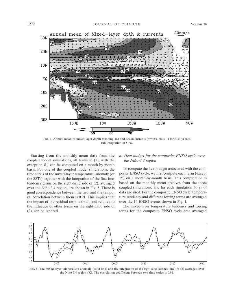
Starting from the monthly mean data from thecoupled model simulations, all terms in (1), with theexception R�, can be computed on a month-by-monthbasis. For one of the coupled model simulations, thetime series of the mixed-layer temperature anomaly (orthe SSTs) together with the integration of the first fourtendency terms on the right-hand side of (2), averagedover the Niño-3.4 region, are shown in Fig. 5. There isgood correspondence between the two, and the tempo-ral correlation between them is 0.91. This implies thatthe impact of the residual term is small, and relative tothe influence of other terms on the right-hand side of(2), can be ignored.

a. Heat budget for the composite ENSO cycle overthe Niño-3.4 region

To compute the heat budget associated with the com-posite ENSO cycle, we first compute each term (exceptR�) on a month-by-month basis. This computation isbased on the monthly mean archives from the threecoupled simulations, and for each simulation 30 yr ofdata are used. For the composite ENSO cycle, tempera-ture tendency and different forcing terms are averagedover the 14 ENSO events shown in Fig. 1.

The mixed-layer temperature tendency and forcingterms for the composite ENSO cycle area averaged

FIG. 5. The mixed-layer temperature anomaly (solid line) and the integration of the right side (dashed line) of (2) averaged overthe Niño-3.4 region (K). The correlation coefficient between two time series is 0.91.

FIG. 4. Annual mean of mixed-layer depth (shading, m) and ocean currents (arrows, cm s�1) for a 30-yr freerun integration of CFS.

1272 J O U R N A L O F C L I M A T E VOLUME 20

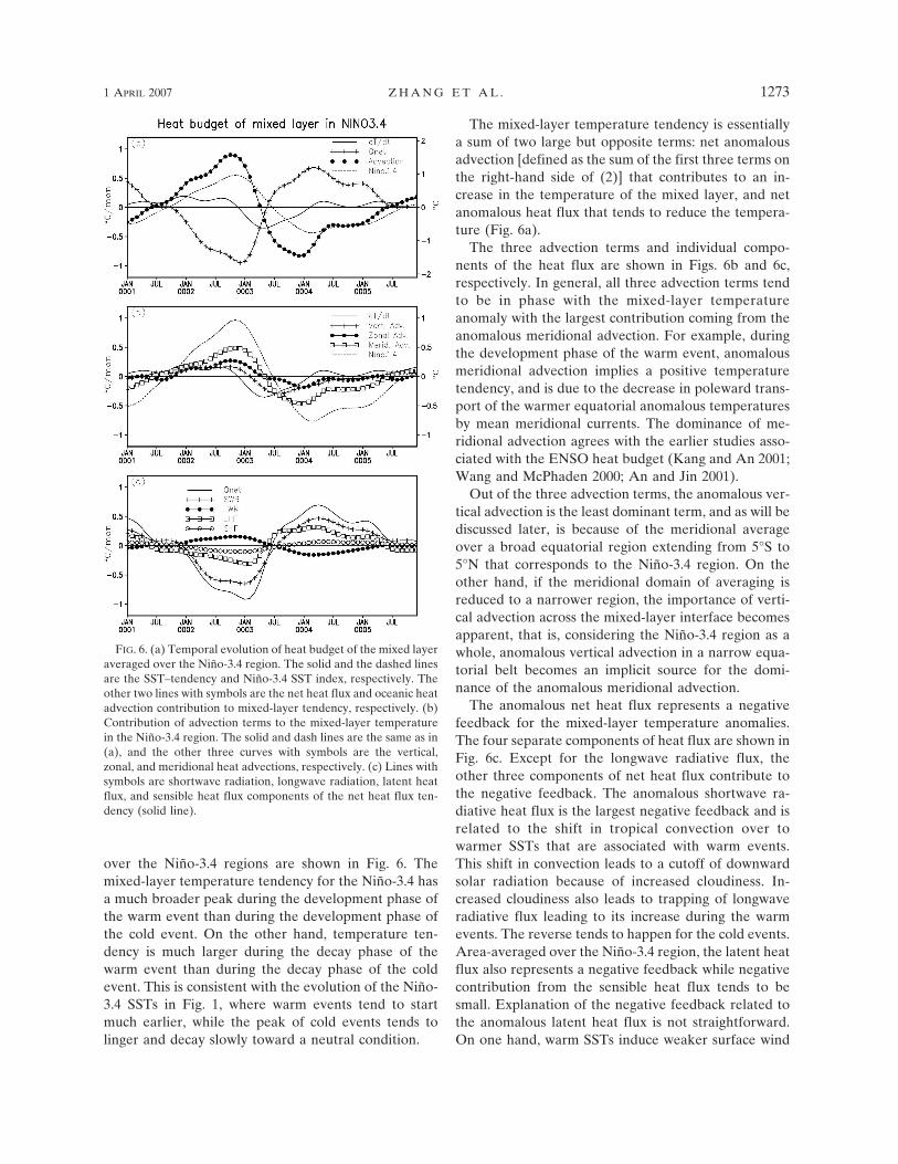
over the Niño-3.4 regions are shown in Fig. 6. Themixed-layer temperature tendency for the Niño-3.4 hasa much broader peak during the development phase ofthe warm event than during the development phase ofthe cold event. On the other hand, temperature ten-dency is much larger during the decay phase of thewarm event than during the decay phase of the coldevent. This is consistent with the evolution of the Niño-3.4 SSTs in Fig. 1, where warm events tend to startmuch earlier, while the peak of cold events tends tolinger and decay slowly toward a neutral condition.

The mixed-layer temperature tendency is essentiallya sum of two large but opposite terms: net anomalousadvection [defined as the sum of the first three terms onthe right-hand side of (2)] that contributes to an in-crease in the temperature of the mixed layer, and netanomalous heat flux that tends to reduce the tempera-ture (Fig. 6a).

The three advection terms and individual compo-nents of the heat flux are shown in Figs. 6b and 6c,respectively. In general, all three advection terms tendto be in phase with the mixed-layer temperatureanomaly with the largest contribution coming from theanomalous meridional advection. For example, duringthe development phase of the warm event, anomalousmeridional advection implies a positive temperaturetendency, and is due to the decrease in poleward trans-port of the warmer equatorial anomalous temperaturesby mean meridional currents. The dominance of me-ridional advection agrees with the earlier studies asso-ciated with the ENSO heat budget (Kang and An 2001;Wang and McPhaden 2000; An and Jin 2001).

Out of the three advection terms, the anomalous ver-tical advection is the least dominant term, and as will bediscussed later, is because of the meridional averageover a broad equatorial region extending from 5°S to5°N that corresponds to the Niño-3.4 region. On theother hand, if the meridional domain of averaging isreduced to a narrower region, the importance of verti-cal advection across the mixed-layer interface becomesapparent, that is, considering the Niño-3.4 region as awhole, anomalous vertical advection in a narrow equa-torial belt becomes an implicit source for the domi-nance of the anomalous meridional advection.

The anomalous net heat flux represents a negativefeedback for the mixed-layer temperature anomalies.The four separate components of heat flux are shown inFig. 6c. Except for the longwave radiative flux, theother three components of net heat flux contribute tothe negative feedback. The anomalous shortwave ra-diative heat flux is the largest negative feedback and isrelated to the shift in tropical convection over towarmer SSTs that are associated with warm events.This shift in convection leads to a cutoff of downwardsolar radiation because of increased cloudiness. In-creased cloudiness also leads to trapping of longwaveradiative flux leading to its increase during the warmevents. The reverse tends to happen for the cold events.Area-averaged over the Niño-3.4 region, the latent heatflux also represents a negative feedback while negativecontribution from the sensible heat flux tends to besmall. Explanation of the negative feedback related tothe anomalous latent heat flux is not straightforward.On one hand, warm SSTs induce weaker surface wind

FIG. 6. (a) Temporal evolution of heat budget of the mixed layeraveraged over the Niño-3.4 region. The solid and the dashed linesare the SST–tendency and Niño-3.4 SST index, respectively. Theother two lines with symbols are the net heat flux and oceanic heatadvection contribution to mixed-layer tendency, respectively. (b)Contribution of advection terms to the mixed-layer temperaturein the Niño-3.4 region. The solid and dash lines are the same as in(a), and the other three curves with symbols are the vertical,zonal, and meridional heat advections, respectively. (c) Lines withsymbols are shortwave radiation, longwave radiation, latent heatflux, and sensible heat flux components of the net heat flux ten-dency (solid line).

1 APRIL 2007 Z H A N G E T A L . 1273

speed as a result of the associated westerly anomalieson top of the mean easterly wind, causing less evapo-ration and thus positive latent heat flux anomalies intothe ocean. On the other hand, warmer SSTs increaseevaporation for a given amplitude of wind speed, lead-ing to negative latent heat flux anomalies into theocean. The net negative latent heat flux anomalies dur-ing the development phase of the warm event in Fig. 6cindicate that the change in latent heat flux due to SSTanomalies dominates over the change due to the sur-face wind speed anomalies.

The analysis of the heat budget so far relates to themixed-layer temperature anomalies averaged over theNiño-3.4 region. In the subsequent analysis, we de-scribe the spatial distribution of different forcing termsin (2). Particularly, we focus on the anomalous advec-tions and also analyze their subcomponents. Since thenet heat flux tends to be a negative feedback to themixed-layer temperature anomalies throughout theENSO cycle, and also throughout the tropical Pacific,for the sake of brevity, results for net heat flux are notshown.

b. Spatial structure of anomalous advections for thecomposite ENSO cycle

The time evolution of mixed-layer tendency and forc-ing terms averaged over the Niño-3.4 region is a suc-cinct way to illustrate the temporal evolution of heatbudget anomalies. To illustrate the spatial evolution ofanomalous advections, a convenient alternative is toextract the mode of variability in the mixed-layer tem-perature tendency that is related to the ENSO cycle,and then to analyze the corresponding spatial patternsfor different tendency terms. This approach is followedto illustrate the spatial variability of anomalous advec-tions.

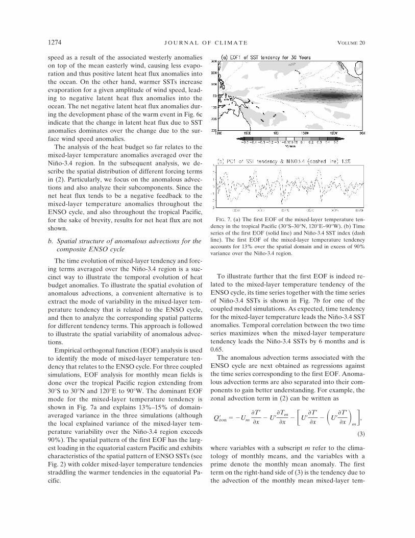
Empirical orthogonal function (EOF) analysis is usedto identify the mode of mixed-layer temperature ten-dency that relates to the ENSO cycle. For three coupledsimulations, EOF analysis for monthly mean fields isdone over the tropical Pacific region extending from30°S to 30°N and 120°E to 90°W. The dominant EOFmode for the mixed-layer temperature tendency isshown in Fig. 7a and explains 13%–15% of domain-averaged variance in the three simulations (althoughthe local explained variance of the mixed-layer tem-perature variability over the Niño-3.4 region exceeds90%). The spatial pattern of the first EOF has the larg-est loading in the equatorial eastern Pacific and exhibitscharacteristics of the spatial pattern of ENSO SSTs (seeFig. 2) with colder mixed-layer temperature tendenciesstraddling the warmer tendencies in the equatorial Pa-cific.

To illustrate further that the first EOF is indeed re-lated to the mixed-layer temperature tendency of theENSO cycle, its time series together with the time seriesof Niño-3.4 SSTs is shown in Fig. 7b for one of thecoupled model simulations. As expected, time tendencyfor the mixed-layer temperature leads the Niño-3.4 SSTanomalies. Temporal correlation between the two timeseries maximizes when the mixed-layer temperaturetendency leads the Niño-3.4 SSTs by 6 months and is0.65.

The anomalous advection terms associated with theENSO cycle are next obtained as regressions againstthe time series corresponding to the first EOF. Anoma-lous advection terms are also separated into their com-ponents to gain better understanding. For example, thezonal advection term in (2) can be written as

Q�zon � �Um

�T�

�x� U�

�Tm

�x� �U�

�T�

�x� �U�

�T�

�x �m�,

�3�

where variables with a subscript m refer to the clima-tology of monthly means, and the variables with aprime denote the monthly mean anomaly. The firstterm on the right-hand side of (3) is the tendency due tothe advection of the monthly mean mixed-layer tem-

FIG. 7. (a) The first EOF of the mixed-layer temperature ten-dency in the tropical Pacific (30°S–30°N, 120°E–90°W). (b) Timeseries of the first EOF (solid line) and Niño-3.4 SST index (dashline). The first EOF of the mixed-layer temperature tendencyaccounts for 13% over the spatial domain and in excess of 90%variance over the Niño-3.4 region.

1274 J O U R N A L O F C L I M A T E VOLUME 20

perature anomaly by the climatological zonal current.The second term on the right-hand side of (3) repre-sents the tendency due to the advection of climatologi-cal mixed-layer temperature by the anomalous monthlymean zonal current. Finally, the last term in (3) is theanomalous nonlinear advection of the monthly meanmixed-layer temperature anomaly by the anomalousmonthly mean zonal currents.

Similar to the decomposition of the zonal advectionterm in (3), the meridional and vertical advection termscan also be written as

Q�mer � �Vm

�T�

�y� V�

�Tm

�y� �V�

�T�

�y� �V�

�T�

�y �m��4�

Q�ver � �Wm

�T�h�z

� W��Thm

�z

� �W��T�h�z

� �W��T�h�z �m

��0.5H

�H�

�t. �5�

In (5), T�h is the temperature anomaly just below themixed layer, while Thm is its climatological value.

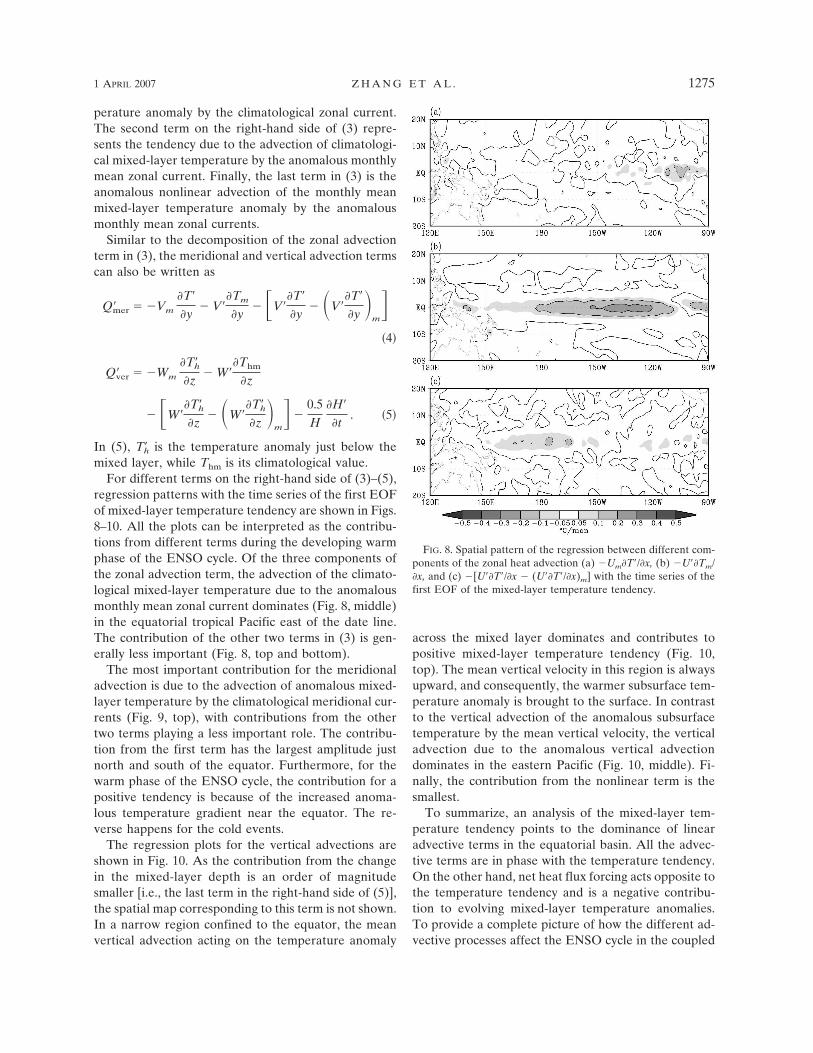
For different terms on the right-hand side of (3)–(5),regression patterns with the time series of the first EOFof mixed-layer temperature tendency are shown in Figs.8–10. All the plots can be interpreted as the contribu-tions from different terms during the developing warmphase of the ENSO cycle. Of the three components ofthe zonal advection term, the advection of the climato-logical mixed-layer temperature due to the anomalousmonthly mean zonal current dominates (Fig. 8, middle)in the equatorial tropical Pacific east of the date line.The contribution of the other two terms in (3) is gen-erally less important (Fig. 8, top and bottom).

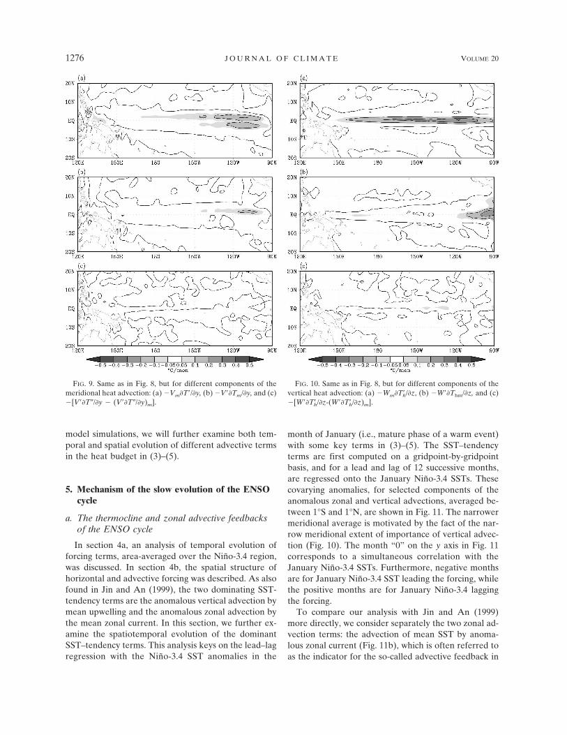
The most important contribution for the meridionaladvection is due to the advection of anomalous mixed-layer temperature by the climatological meridional cur-rents (Fig. 9, top), with contributions from the othertwo terms playing a less important role. The contribu-tion from the first term has the largest amplitude justnorth and south of the equator. Furthermore, for thewarm phase of the ENSO cycle, the contribution for apositive tendency is because of the increased anoma-lous temperature gradient near the equator. The re-verse happens for the cold events.

The regression plots for the vertical advections areshown in Fig. 10. As the contribution from the changein the mixed-layer depth is an order of magnitudesmaller [i.e., the last term in the right-hand side of (5)],the spatial map corresponding to this term is not shown.In a narrow region confined to the equator, the meanvertical advection acting on the temperature anomaly

across the mixed layer dominates and contributes topositive mixed-layer temperature tendency (Fig. 10,top). The mean vertical velocity in this region is alwaysupward, and consequently, the warmer subsurface tem-perature anomaly is brought to the surface. In contrastto the vertical advection of the anomalous subsurfacetemperature by the mean vertical velocity, the verticaladvection due to the anomalous vertical advectiondominates in the eastern Pacific (Fig. 10, middle). Fi-nally, the contribution from the nonlinear term is thesmallest.

To summarize, an analysis of the mixed-layer tem-perature tendency points to the dominance of linearadvective terms in the equatorial basin. All the advec-tive terms are in phase with the temperature tendency.On the other hand, net heat flux forcing acts opposite tothe temperature tendency and is a negative contribu-tion to evolving mixed-layer temperature anomalies.To provide a complete picture of how the different ad-vective processes affect the ENSO cycle in the coupled

FIG. 8. Spatial pattern of the regression between different com-ponents of the zonal heat advection (a) �UmT�/x, (b) �U�Tm/x, and (c) �[U�T�/x � (U�T�/x)m] with the time series of thefirst EOF of the mixed-layer temperature tendency.

1 APRIL 2007 Z H A N G E T A L . 1275

model simulations, we will further examine both tem-poral and spatial evolution of different advective termsin the heat budget in (3)–(5).

5. Mechanism of the slow evolution of the ENSOcycle

a. The thermocline and zonal advective feedbacksof the ENSO cycle

In section 4a, an analysis of temporal evolution offorcing terms, area-averaged over the Niño-3.4 region,was discussed. In section 4b, the spatial structure ofhorizontal and advective forcing was described. As alsofound in Jin and An (1999), the two dominating SST-tendency terms are the anomalous vertical advection bymean upwelling and the anomalous zonal advection bythe mean zonal current. In this section, we further ex-amine the spatiotemporal evolution of the dominantSST–tendency terms. This analysis keys on the lead–lagregression with the Niño-3.4 SST anomalies in the

month of January (i.e., mature phase of a warm event)with some key terms in (3)–(5). The SST–tendencyterms are first computed on a gridpoint-by-gridpointbasis, and for a lead and lag of 12 successive months,are regressed onto the January Niño-3.4 SSTs. Thesecovarying anomalies, for selected components of theanomalous zonal and vertical advections, averaged be-tween 1°S and 1°N, are shown in Fig. 11. The narrowermeridional average is motivated by the fact of the nar-row meridional extent of importance of vertical advec-tion (Fig. 10). The month “0” on the y axis in Fig. 11corresponds to a simultaneous correlation with theJanuary Niño-3.4 SSTs. Furthermore, negative monthsare for January Niño-3.4 SST leading the forcing, whilethe positive months are for January Niño-3.4 laggingthe forcing.

To compare our analysis with Jin and An (1999)more directly, we consider separately the two zonal ad-vection terms: the advection of mean SST by anoma-lous zonal current (Fig. 11b), which is often referred toas the indicator for the so-called advective feedback in

FIG. 9. Same as in Fig. 8, but for different components of themeridional heat advection: (a) �VmT�/y, (b) �V�Tm/y, and (c)�[V�T/y � (V�T/y)m].

FIG. 10. Same as in Fig. 8, but for different components of thevertical heat advection: (a) �WmT�h/z, (b) �W�Thm/z, and (c)�[W�T�h/z-(W�T�h/z)m].

1276 J O U R N A L O F C L I M A T E VOLUME 20

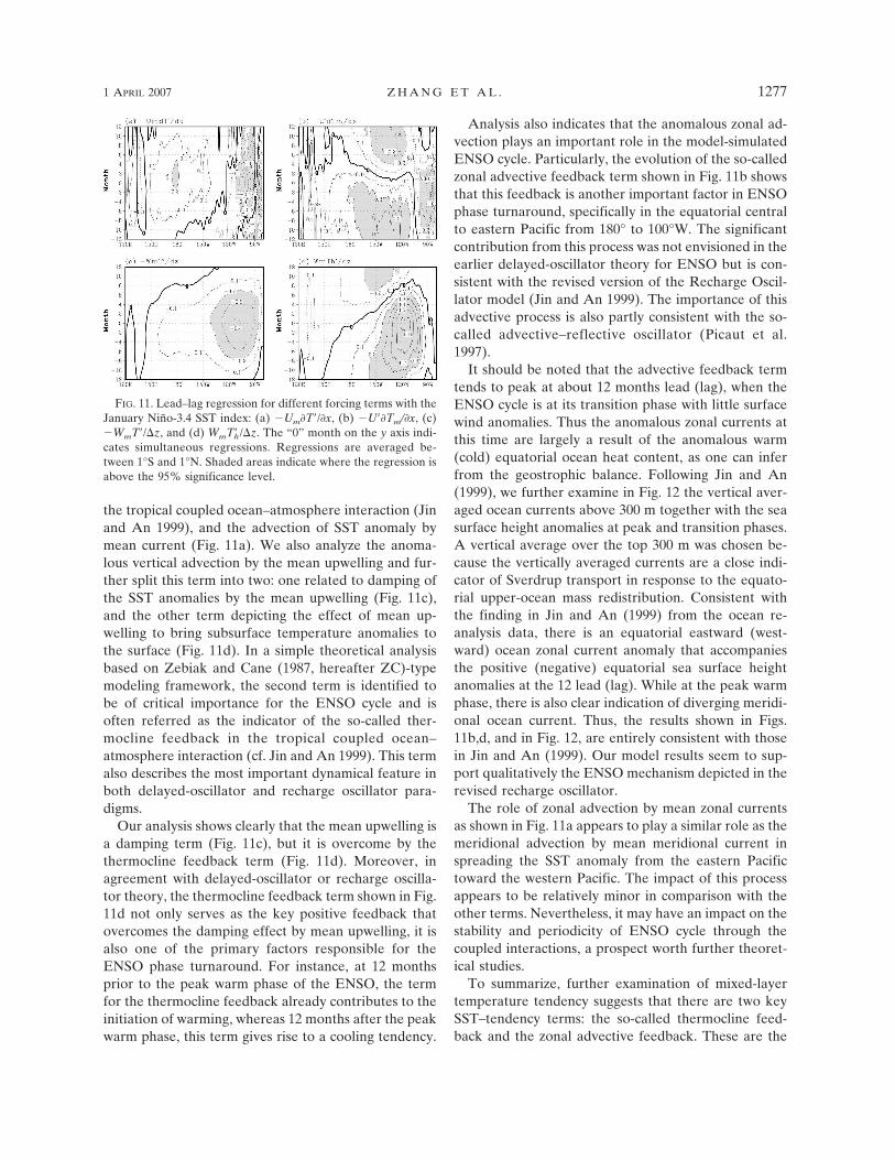
the tropical coupled ocean–atmosphere interaction (Jinand An 1999), and the advection of SST anomaly bymean current (Fig. 11a). We also analyze the anoma-lous vertical advection by the mean upwelling and fur-ther split this term into two: one related to damping ofthe SST anomalies by the mean upwelling (Fig. 11c),and the other term depicting the effect of mean up-welling to bring subsurface temperature anomalies tothe surface (Fig. 11d). In a simple theoretical analysisbased on Zebiak and Cane (1987, hereafter ZC)-typemodeling framework, the second term is identified tobe of critical importance for the ENSO cycle and isoften referred as the indicator of the so-called ther-mocline feedback in the tropical coupled ocean–atmosphere interaction (cf. Jin and An 1999). This termalso describes the most important dynamical feature inboth delayed-oscillator and recharge oscillator para-digms.

Our analysis shows clearly that the mean upwelling isa damping term (Fig. 11c), but it is overcome by thethermocline feedback term (Fig. 11d). Moreover, inagreement with delayed-oscillator or recharge oscilla-tor theory, the thermocline feedback term shown in Fig.11d not only serves as the key positive feedback thatovercomes the damping effect by mean upwelling, it isalso one of the primary factors responsible for theENSO phase turnaround. For instance, at 12 monthsprior to the peak warm phase of the ENSO, the termfor the thermocline feedback already contributes to theinitiation of warming, whereas 12 months after the peakwarm phase, this term gives rise to a cooling tendency.

Analysis also indicates that the anomalous zonal ad-vection plays an important role in the model-simulatedENSO cycle. Particularly, the evolution of the so-calledzonal advective feedback term shown in Fig. 11b showsthat this feedback is another important factor in ENSOphase turnaround, specifically in the equatorial centralto eastern Pacific from 180° to 100°W. The significantcontribution from this process was not envisioned in theearlier delayed-oscillator theory for ENSO but is con-sistent with the revised version of the Recharge Oscil-lator model (Jin and An 1999). The importance of thisadvective process is also partly consistent with the so-called advective–reflective oscillator (Picaut et al.1997).

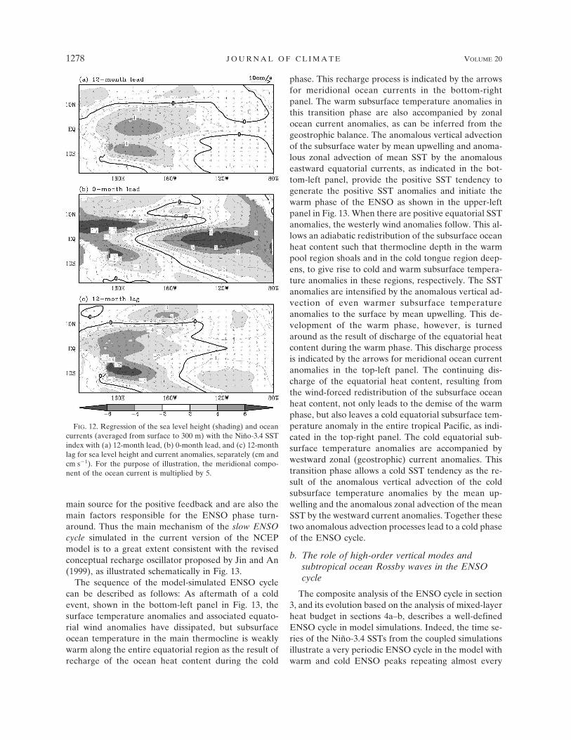
It should be noted that the advective feedback termtends to peak at about 12 months lead (lag), when theENSO cycle is at its transition phase with little surfacewind anomalies. Thus the anomalous zonal currents atthis time are largely a result of the anomalous warm(cold) equatorial ocean heat content, as one can inferfrom the geostrophic balance. Following Jin and An(1999), we further examine in Fig. 12 the vertical aver-aged ocean currents above 300 m together with the seasurface height anomalies at peak and transition phases.A vertical average over the top 300 m was chosen be-cause the vertically averaged currents are a close indi-cator of Sverdrup transport in response to the equato-rial upper-ocean mass redistribution. Consistent withthe finding in Jin and An (1999) from the ocean re-analysis data, there is an equatorial eastward (west-ward) ocean zonal current anomaly that accompaniesthe positive (negative) equatorial sea surface heightanomalies at the 12 lead (lag). While at the peak warmphase, there is also clear indication of diverging meridi-onal ocean current. Thus, the results shown in Figs.11b,d, and in Fig. 12, are entirely consistent with thosein Jin and An (1999). Our model results seem to sup-port qualitatively the ENSO mechanism depicted in therevised recharge oscillator.

The role of zonal advection by mean zonal currentsas shown in Fig. 11a appears to play a similar role as themeridional advection by mean meridional current inspreading the SST anomaly from the eastern Pacifictoward the western Pacific. The impact of this processappears to be relatively minor in comparison with theother terms. Nevertheless, it may have an impact on thestability and periodicity of ENSO cycle through thecoupled interactions, a prospect worth further theoret-ical studies.

To summarize, further examination of mixed-layertemperature tendency suggests that there are two keySST–tendency terms: the so-called thermocline feed-back and the zonal advective feedback. These are the

FIG. 11. Lead–lag regression for different forcing terms with theJanuary Niño-3.4 SST index: (a) �UmT�/x, (b) �U�Tm/x, (c)�WmT�/�z, and (d) WmT�h/�z. The “0” month on the y axis indi-cates simultaneous regressions. Regressions are averaged be-tween 1°S and 1°N. Shaded areas indicate where the regression isabove the 95% significance level.

1 APRIL 2007 Z H A N G E T A L . 1277

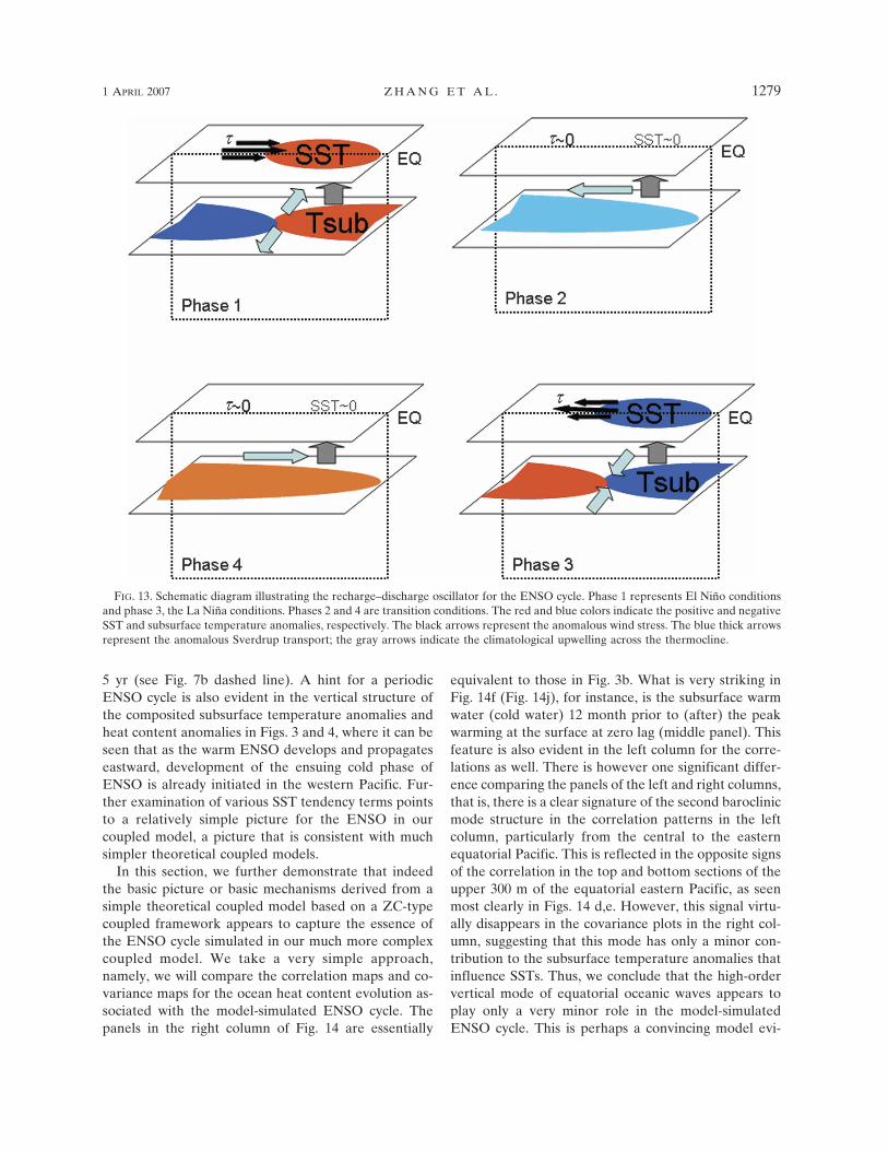
main source for the positive feedback and are also themain factors responsible for the ENSO phase turn-around. Thus the main mechanism of the slow ENSOcycle simulated in the current version of the NCEPmodel is to a great extent consistent with the revisedconceptual recharge oscillator proposed by Jin and An(1999), as illustrated schematically in Fig. 13.

The sequence of the model-simulated ENSO cyclecan be described as follows: As aftermath of a coldevent, shown in the bottom-left panel in Fig. 13, thesurface temperature anomalies and associated equato-rial wind anomalies have dissipated, but subsurfaceocean temperature in the main thermocline is weaklywarm along the entire equatorial region as the result ofrecharge of the ocean heat content during the cold

phase. This recharge process is indicated by the arrowsfor meridional ocean currents in the bottom-rightpanel. The warm subsurface temperature anomalies inthis transition phase are also accompanied by zonalocean current anomalies, as can be inferred from thegeostrophic balance. The anomalous vertical advectionof the subsurface water by mean upwelling and anoma-lous zonal advection of mean SST by the anomalouseastward equatorial currents, as indicated in the bot-tom-left panel, provide the positive SST tendency togenerate the positive SST anomalies and initiate thewarm phase of the ENSO as shown in the upper-leftpanel in Fig. 13. When there are positive equatorial SSTanomalies, the westerly wind anomalies follow. This al-lows an adiabatic redistribution of the subsurface oceanheat content such that thermocline depth in the warmpool region shoals and in the cold tongue region deep-ens, to give rise to cold and warm subsurface tempera-ture anomalies in these regions, respectively. The SSTanomalies are intensified by the anomalous vertical ad-vection of even warmer subsurface temperatureanomalies to the surface by mean upwelling. This de-velopment of the warm phase, however, is turnedaround as the result of discharge of the equatorial heatcontent during the warm phase. This discharge processis indicated by the arrows for meridional ocean currentanomalies in the top-left panel. The continuing dis-charge of the equatorial heat content, resulting fromthe wind-forced redistribution of the subsurface oceanheat content, not only leads to the demise of the warmphase, but also leaves a cold equatorial subsurface tem-perature anomaly in the entire tropical Pacific, as indi-cated in the top-right panel. The cold equatorial sub-surface temperature anomalies are accompanied bywestward zonal (geostrophic) current anomalies. Thistransition phase allows a cold SST tendency as the re-sult of the anomalous vertical advection of the coldsubsurface temperature anomalies by the mean up-welling and the anomalous zonal advection of the meanSST by the westward current anomalies. Together thesetwo anomalous advection processes lead to a cold phaseof the ENSO cycle.

b. The role of high-order vertical modes andsubtropical ocean Rossby waves in the ENSOcycle

The composite analysis of the ENSO cycle in section3, and its evolution based on the analysis of mixed-layerheat budget in sections 4a–b, describes a well-definedENSO cycle in model simulations. Indeed, the time se-ries of the Niño-3.4 SSTs from the coupled simulationsillustrate a very periodic ENSO cycle in the model withwarm and cold ENSO peaks repeating almost every

FIG. 12. Regression of the sea level height (shading) and oceancurrents (averaged from surface to 300 m) with the Niño-3.4 SSTindex with (a) 12-month lead, (b) 0-month lead, and (c) 12-monthlag for sea level height and current anomalies, separately (cm andcm s�1). For the purpose of illustration, the meridional compo-nent of the ocean current is multiplied by 5.

1278 J O U R N A L O F C L I M A T E VOLUME 20

5 yr (see Fig. 7b dashed line). A hint for a periodicENSO cycle is also evident in the vertical structure ofthe composited subsurface temperature anomalies andheat content anomalies in Figs. 3 and 4, where it can beseen that as the warm ENSO develops and propagateseastward, development of the ensuing cold phase ofENSO is already initiated in the western Pacific. Fur-ther examination of various SST tendency terms pointsto a relatively simple picture for the ENSO in ourcoupled model, a picture that is consistent with muchsimpler theoretical coupled models.

In this section, we further demonstrate that indeedthe basic picture or basic mechanisms derived from asimple theoretical coupled model based on a ZC-typecoupled framework appears to capture the essence ofthe ENSO cycle simulated in our much more complexcoupled model. We take a very simple approach,namely, we will compare the correlation maps and co-variance maps for the ocean heat content evolution as-sociated with the model-simulated ENSO cycle. Thepanels in the right column of Fig. 14 are essentially

equivalent to those in Fig. 3b. What is very striking inFig. 14f (Fig. 14j), for instance, is the subsurface warmwater (cold water) 12 month prior to (after) the peakwarming at the surface at zero lag (middle panel). Thisfeature is also evident in the left column for the corre-lations as well. There is however one significant differ-ence comparing the panels of the left and right columns,that is, there is a clear signature of the second baroclinicmode structure in the correlation patterns in the leftcolumn, particularly from the central to the easternequatorial Pacific. This is reflected in the opposite signsof the correlation in the top and bottom sections of theupper 300 m of the equatorial eastern Pacific, as seenmost clearly in Figs. 14 d,e. However, this signal virtu-ally disappears in the covariance plots in the right col-umn, suggesting that this mode has only a minor con-tribution to the subsurface temperature anomalies thatinfluence SSTs. Thus, we conclude that the high-ordervertical mode of equatorial oceanic waves appears toplay only a very minor role in the model-simulatedENSO cycle. This is perhaps a convincing model evi-

FIG. 13. Schematic diagram illustrating the recharge–discharge oscillator for the ENSO cycle. Phase 1 represents El Niño conditionsand phase 3, the La Niña conditions. Phases 2 and 4 are transition conditions. The red and blue colors indicate the positive and negativeSST and subsurface temperature anomalies, respectively. The black arrows represent the anomalous wind stress. The blue thick arrowsrepresent the anomalous Sverdrup transport; the gray arrows indicate the climatological upwelling across the thermocline.

1 APRIL 2007 Z H A N G E T A L . 1279

Fig 13 live 4/C

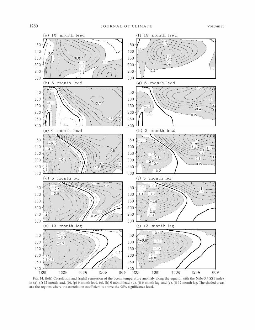
FIG. 14. (left) Correlation and (right) regression of the ocean temperature anomaly along the equator with the Niño-3.4 SST indexin (a), (f) 12-month lead, (b), (g) 6-month lead, (c), (h) 0-month lead, (d), (i) 6-month lag, and (e), (j) 12-month lag. The shaded areasare the regions where the correlation coefficient is above the 95% significance level.

1280 J O U R N A L O F C L I M A T E VOLUME 20

dence in support of the relevance of the simple ZC-typeframework in which only the first baroclinic mode ofequatorial wave dynamics is captured.

We extended a similar analysis by contrasting thecorrelation and covariance maps for the horizontalstructures of upper-ocean heat content evolution. Themain difference between the two, showed in Fig. 15, liesin the off-equatorial regions poleward of 15°S to 15°N.The correlation signal in the subtropical region, al-though weak, has a clear westward propagation and is aconsequence of the subtropical ocean Rossby waves.From the contrast between the panels on the right andleft in Fig. 15, it is clear that the subtropical Rossbywaves, no matter whether they are forced by wind stresscurl in the subtropical region, or are reflected at theeastern boundary from the equatorial Kelvin waves,contribute little to changes in the equatorial heat con-tent, such as discharging and recharging of the equato-rial heat content. Thus our simple analysis appears tobe consistent with the finding from the analysis of thesimple ZC-type model that ocean Rossby waves be-yond 15°N and 15°S appear to be slaved to the ENSOcycle and do not actively contribute to the evolution ofthe ENSO cycle (e.g., Battisti 1988; Jin 1997b).

Although it is known from theoretical modeling thatthe higher-order vertical modes and subtropical oceanRossby waves play little role in the ENSO cycle, wehave demonstrated with a simple diagnostic methodthat this is also the case for the ENSO cycles simulatedin the complex coupled model. Thus, the ENSO cyclessimulated in our comprehensive coupled model shareessentially the ENSO dynamics depicted in simplecoupled models.

6. Summary and discussion

Based on a set of coupled model simulations, in thispaper the evolution of model-simulated ENSO wasanalyzed. The analysis is of importance for at least thefollowing two reasons: 1) coupled models are increas-ingly used to provide guidance for seasonal predictions,and for their optimal utilization, it is essential to under-stand the mechanisms (and biases) behind the model-simulated ENSO events; and 2) multiple theories forENSO evolution have been proposed, and reliance oncoupled models is an essential tool for understandingthe relative importance of different ENSO mecha-nisms.

Our analysis was based on the evolution of compositeENSO events as well as on the analysis of the mixed-layer heat budget associated with ENSOs. The salientfeatures of the model-simulated ENSO cycle were asfollows:

• For the composite ENSO cycle simulated by thecoupled model, the onset of warm ENSO events oc-curs approximately 6 months earlier than in the ob-servations. This earlier onset is perhaps related to thefact that a model-simulated ENSO has a period ofaround 5 yr instead of about 4 yr in the observations.

• The heat budget of the mixed layer is primarily a sumof two large, but opposite terms: advections and thenet surface heat flux.

• The net surface heat flux represents a damping term,that is, is opposite to the sign of the mixed-layer tem-perature anomaly. The largest term in the surfaceheat flux is the anomalous shortwave radiative heatflux.

• Among different advection terms, linear advectionterms dominate. Zonal advection is dominated by theadvection of climatological mixed-layer temperaturedue to the anomalous zonal currents. For the meridi-onal advection, the most important contribution is bythe advection of anomalous mixed-layer temperatureby the climatological meridional ocean currents. Thisterm is responsible for the meridional spread of equa-torial SST anomalies. The anomalous vertical advec-tion is narrowly confined to an equatorial strip andoccurs because of the mean upwelling of the tem-perature anomaly below the mixed layer.

• The model simulations have a well-defined, and avery periodic, ENSO cycle. For example, almost allwarm ENSO events are followed by cold ENSOevents, and the cycle tends to repeat every 5 yr.

• The main positive feedback mechanism appears fromthe so-called thermocline feedback. Namely, warm(cold) equatorial SST anomalies gives rise to westerly(easterly) wind anomalies to the west of the SSTanomaly; the latter produce warm (cold) subsurfaceocean temperature anomalies by pressing down theisothermal surface (or thermocline depth) throughadiabatic mass adjustment; and finally, these warm(cold) subsurface temperature anomalies are broughtup to the surface by the mean upwelling to reinforcethe SST anomalies.

• The ENSO phase transition largely results from twoprocesses: the anomalous zonal advection of meanSST by anomalous zonal currents and anomalous ver-tical advection by mean upwelling, which brings thesubsurface temperature anomalies to the surface.During the warm (cold) to cold (warm) ENSO phasetransition, the equatorial subsurface oceanic tem-perature anomalies along the entire equator are al-ready cold (warm) owing to the excessive discharge(recharge) during the warm (cold) phase. This cold(warm) equatorial subsurface temperature anomalyis also accompanied by anomalous eastward (west-

1 APRIL 2007 Z H A N G E T A L . 1281

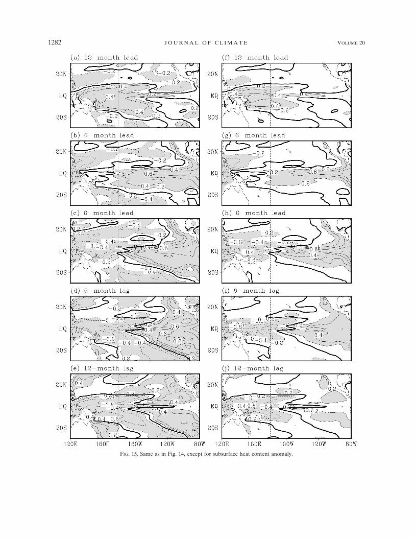
FIG. 15. Same as in Fig. 14, except for subsurface heat content anomaly.

1282 J O U R N A L O F C L I M A T E VOLUME 20

ward) equatorial zonal current anomalies. Both thecold (warm) equatorial subsurface temperature andeastward (westward) zonal currents bring a warm tocold (cold to warm) ENSO phase transition. Thusmodel-simulated ENSO mechanisms are largely con-sistent with the revised recharge oscillator model ofJin and An (1999).

• Our analysis also lends further support that high-order vertical modes and subtropical ocean Rossbywaves play little role in the ENSO cycles. Overall, theENSO simulated in the complex model shares similarmechanisms identified in the much simpler coupledmodels.

The coupled model analyzed in this study has largerthan observed high-frequency atmospheric noise (orvariability), and associated phenomena, for example,westerly wind events. For instance the variance of in-traseasonal variability is significantly larger than what isobserved (not shown). This high-frequency variabilitysimulated in the coupled model seems to have littleconsequence on the evolution of the model-simulatedENSO cycle (Wang et al. 2005) and is probably a resultof the dominant role of coupled ocean–atmosphere in-teractions and their control on the model-simulatedENSO cycle.

There are still a number of issues that remain un-clear. For instance, what controls the periodicity of theENSO cycle? Why it is around 5 yr and why is it soregular even in the presence of a considerable amountof high-frequency noise? ENSO simulations by otherCGCMs have also been analyzed in a number of studies(Latif et al. 2001; AchutaRao and Sperber 2001; Dele-cluse et al. 1998). Overall, in most CGCMs the simu-lated ENSOs are either too weak in amplitude or occurtoo frequently. In addition, many models fail to repro-duce the observed seasonal phase locking of ENSOevents that generally tends to peak near the end of thecalendar year. In contrast, the NCEP CFS realisticallycaptured the seasonal phase locking, but with strongeramplitude and a longer period. However, as for manyother coupled CGCMs, the simulated interannual vari-ability in the western Pacific (far eastern Pacific) in theNCEP CFS was too strong (weak). The reasons for thedeficiencies of this coupled model remain unclear. Fur-ther analysis of the coupled model simulations togetherwith some sensitivity of simulated ENSO to the climatemean state may provide further insight into some ofthese questions.

Acknowledgments. Support provided by the NOAAOGP’s “Climate Dynamics and Experimental Predic-tion” program is gratefully acknowledged. FFJ is sup-

ported by NSF Grant ATM-0226141 and NOAA GrantGC01- 246.

REFERENCES

AchutaRao, K., and K. R. Sperber, 2001: Simulation of the ElNiño Southern Oscillation: Results from the Coupled ModelIntercomparison Project. Climate Dyn., 19, 191–209.

An, S.-I., and F.-F. Jin, 2001: Collective role of thermocline andzonal advective feedbacks in the ENSO mode. J. Climate, 14,3421–3432.

Battisti, D. S., 1988: The dynamics and thermodynamics of awarming event in a coupled tropical atmosphere–oceanmodel. J. Atmos. Sci., 45, 2889–2919.

——, and A. C. Hirst, 1989: Interannual variability in the tropicalatmosphere ocean system: Influence of the basic state andocean geometry. J. Atmos. Sci., 46, 1687–1712.

Bjerknes, J., 1969: Atmospheric teleconnections from the equa-torial Pacific. Mon. Wea. Rev., 97, 163–172.

Bonjean, F., 2001: Influence of surface currents on the sea surfacetemperature in the tropical Pacific Ocean. J. Phys. Oceanogr.,31, 943–961.

——, and G. S. E. Lagerloef, 2002: Diagnostic model and analysisof the surface currents in the tropical Pacific Ocean. J. Phys.Oceanogr., 32, 2938–2954.

Delcroix, T., J.-P. Boulanger, F. Masia, and C. Menkes, 1994:Geosat-derived sea level and surface current anomalies in theequatorial Pacific during the 1986–1989 El Niño and La Niña.J. Geophys. Res., 99, 25 093–25107.

Delecluse, P., M. K. Davey, Y. Kitamura, S. G. H. Philander, M.Suarez, and L. Bengtsson, 1998: Coupled general circulationmodeling of the tropical Pacific. J. Geophys. Res., 103,14 357–14 373.

Frankignoul, C., F. Bonjean, and G. Reverdin, 1996: Interannualvariability of surface currents in the tropical Pacific during1987–1993. J. Geophys. Res., 101, 3629–3647.

Gent, P. R., and J. C. McWilliams, 1990: Isopycnal mixing inocean circulation models. J. Phys. Oceanogr., 20, 150–155.

Griffies, S. M., A. Gnanadesikan, R. C. Pacanaowski, V. Larichev,J. K. Dukowicz, and R. D. Smith, 1998: Isoneutral diffusionin a z-coordinate ocean model. J. Phys. Oceanogr., 28, 805–830.

Hasegawa, T., and K. Hanawa, 2003: Heat content variability re-lated to ENSO events in the Pacific. J. Phys. Oceanogr., 33,407–421.

Hayes, S. P., L. J. Mangum, J. Picaut, A. Sumi, and K. Takeuchi,1991: TOGA-TAO: A moored array for real-time measure-ments in the tropical Pacific Ocean. Bull. Amer. Meteor. Soc.,72, 339–347.

Hirst, A. C., 1988: Slow instabilities in tropical ocean basin–globalatmosphere models. J. Atmos. Sci., 45, 830–852.

Jin, F.-F., 1996: Tropical ocean-atmosphere interaction, the Pa-cific cold tongue, and the El Niño Southern Oscillation. Sci-ence, 274, 76–78.

——, 1997a: An equatorial ocean recharge paradigm for ENSO.Part I: Conceptual model. J. Atmos. Sci., 54, 811–829.

——, 1997b: An equatorial ocean recharge paradigm for ENSO.Part II: A stripped-down coupled model. J. Atmos. Sci., 54,830–847.

——, and S.-I. An, 1999: Thermocline and zonal advective feed-backs within the equatorial ocean recharge oscillator modelfor ENSO. Geophys. Res. Lett., 26, 2989–2992.

Kanamitsu, M., W. Ebisuzaki, J. Woollen, S.-K. Yang, J. J. Slingo,

1 APRIL 2007 Z H A N G E T A L . 1283

M. Fiorino, and G. L. Potter, 2002: NCEP–DOE AMIP-IIReanalysis (R-2). Bull. Amer. Meteor. Soc., 83, 1631–1643.

Kang, I.-S., and S.-I. An, 2001: A systematic approximation of theSST anomaly equation for ENSO. J. Meteor. Soc. Japan, 79,1–10.

Kessler, W. S., and M. J. McPhaden, 1995: Oceanic equatorialwaves and the 1991–93 El Niño. J. Climate, 8, 1057–1072.

Large, W. G., J. C. McWilliams, and S. C. Doney, 1994: Oceanicvertical mixing: A review and a model with nonlocal bound-ary layer parameterization. Rev. Geophys., 32, 363–403.

Latif, M., and Coauthors, 2001: ENSIP: The El Nino simulationintercomparison project. Climate Dyn., 18, 255–276.

Lau, N. C., S. G. H. Philander, and M. J. Nath, 1992: Simulation ofENSO-like phenomena with a law-resolution coupled GCMof the global ocean and atmosphere. J. Climate, 5, 284–307.

Levitus, S., and T. P. Boyer, 1994: Temperature. Vol. 4, WorldOcean Atlas 1994, NOAA Atlas NESDIS 4, 117 pp.

McPhaden, M. J., and J. Picaut, 1990: El Niño–Southern Oscilla-tion displacements of the western equatorial Pacific warmpool. Science, 250, 1385–1388.

Pacanowski, R. C., and S. M. Griffies, 1998: MOM 3.0 Manual.NOAA/Geophysical Fluid Dynamics Laboratory, 680 pp.

Philander, S. G. H., 1990: El Niño, La Niña and the SouthernOscillation. Academic Press, 293 pp.

Picaut, J., M. Ioualalen, C. Menkes, T. Delcroix, and M. J.McPhaden, 1996: Mechanism of the zonal displacements ofthe Pacific warm pool: Implications for ENSO. Science, 274,1486–1489.

——, F. Masia, and Y. duPenhoat, 1997: An advective–reflectiveconceptual model for the oscillatory nature of ENSO. Sci-ence, 277, 663–666.

Rasmusson, E. M., and T. H. Carpenter, 1982: Variations in tropi-cal sea surface temperature and surface wind fields associatedwith the Southern Oscillation–El Niño. Mon. Wea. Rev., 110,354–384.

Saha, S., and Coauthors, 2006: The NCEP Climate Forecast Sys-tem. J. Climate, 19, 3483–3517.

Smagorinsky, J., 1963: General circulation experiments with theprimitive equations: I. The basic experiment. Mon. Wea.Rev., 91, 99–164.

Solomon, A., and F.-F. Jin, 2005: A study of the impact of off-equatorial warm pool SST anomalies on ENSO cycles. J. Cli-mate, 18, 274–286.

Suarez, M. J., and P. S. Schopf, 1988: A delayed action oscillatorfor ENSO. J. Atmos. Sci., 45, 3283–3287.

Vialard, J., C. Menkes, J. P. Boulanger, P. Delecluse, E. Guil-yardi, M. J. McPhaden, and G. Madec, 2001: A model studyof oceanic mechanisms affecting equatorial Pacific sea sur-face temperature during the 1997–98 El Niño. J. Phys. Ocean-ogr., 31, 1649–1675.

Wang, B., and Q. Zhang, 2002: Pacific–East Asian teleconnection.Part II: How the Philippine Sea anomalous anticyclone isestablished during El Niño development. J. Climate, 15,3252–3265.

——, R. Wu, and R. Lukas, 2000: Annual adjustment of the ther-mocline in the tropical Pacific Ocean. J. Climate, 13, 596–616.

Wang, C., and R. H. Weisberg, 1994: On the “slow mode” mecha-nism in ENSO-related coupled ocean–atmosphere models. J.Climate, 7, 1657–1667.

——, and J. Picaut, 2004: Understanding ENSO physics—A re-view. Earth’s Climate: The Ocean-Atmosphere Interaction,Geophys. Monogr., Vol. 147, Amer. Geophys. Union, 21–48.

Wang, W., and M. J. McPhaden, 2000: The surface-layer heat bal-ance in the equatorial Pacific Ocean. Part II: Interannualvariability. J. Phys. Oceanogr., 30, 2989–3008.

——, S. Saha, H. L. Pan, S. Nadiga, and G. White, 2005: Simula-tion of ENSO in the new NCEP Coupled Forecast SystemModel (CFS03). Mon. Wea. Rev., 133, 1574–1593.

Weisberg, R. H., and C. Wang, 1997: Slow variability in the equa-torial west-central Pacific in relation to ENSO. J. Climate, 10,1998–2017.

Wyrtki, K., 1975: El Niño—The dynamic response of the equato-rial Pacific Ocean to atmospheric forcing. J. Phys. Oceanogr.,5, 91–103.

Yu, J. Y., and C. R. Mechoso, 2001: A coupled atmosphere–oceanGCM study of the ENSO cycle. J. Climate, 14, 2329–2350.

Zebiak, S. E., and M. A. Cane, 1987: A model El Niño–SouthernOscillation. Mon. Wea. Rev., 115, 2262–2278.

1284 J O U R N A L O F C L I M A T E VOLUME 20